Population Models

Modeling and Simulation I-2012

Content

1. Basic Population Model2. One population

A. Exponential growthB. Logistic growthC. Linear growthD. Stochastic Population Dynamics ModelingE. Real Human Populations

3. Two populationsA. Lotka-Volterra B. Kolgomrov

What is Demography?

The scientific study of the changing size, composition and spatial distribution of a human population and the processes which shape them. Is concerned with:Population size Population growth or declinePopulation processes Population distributionPopulation structure Population characteristics

1. Basic Population Model

Basic Population Model

)(

)(

Nfdt

dN

Nft

N

N(t)

N(t): Population sizeNumber of individuals in the population

Historical Context

The starting point for population growth models is The Principle of Population, published in 1798 by Thomas R. Malthus (1766-1834). In it he presented his theories of human population growth and relationships between over-population and misery. The model he used is now called the exponential model of population growth. 

In 1846, Pierre Francois Verhulst, a Belgian scientist, proposed that population growth depends not only on the population size but also on the effect of a “carrying capacity” that would limit growth. His formula is now called the "logistic model" or the Verhulst model.

Recent DevelopmentsMost recently, the logistic equation has

been used as part of exploration of what is called "chaos theory". Most of this work was collected for the first time by Robert May in a classic article published in Nature in June of 1976. Robert May started his career as a physicist but then did his post-doctoral work in applied mathematics. He became very interested in the mathematical explanations of what enables competing species to coexist and then in the mathematics behind populations growth.

Stochastic Population Dynamics Modeling

2. Relevant Models

Exponential growth

Logistic growth

Linear growth

Stochastic Population Dynamics Modeling

A. Exponential growth

pop. size at time

t+t=

pop. size at time

t+

growth increment

N(t+ t) = N(t) + N

Hypothesis: N = r N t

r - rate constant of growth

Differential equation for exponential growth

rNdtdN

)exp()( 0 rtNtN

0 2 4 6 8 10 12 14 16 18 200

1

2

3

4

5

6

7

8

9

10

Time - t

N(t)

Exponential growth r=0.1

Exponential growth in discrete time

Nt+1 = Nt + r Nt

Nt+1 = (1+r) Nt

Nt = (1+r)t N0

Exponential decline

rNdtdN

)exp()( 0 rtNtN

r - mortality rate

0 2 4 6 8 10 12 14 16 18 200

20

40

60

80

100

120

Time – t

N(t)

Exponential decline r=0.1

B. Logistic growth model

Relies on the hypothesis that population growth is limited by environmental capacity

K

NrN

dt

dN1

K – environmental capacity

Differential equation for Logistic growth

As this shows, the curve produced by the logistic difference equation is S-shaped. Initially there is an exponential growth phase, but as growth gets closer to the carrying capacity (more or less at time step 37 in this case), the growth slows down and the population asymptotically approaches capacity.

Nt+1 = Nt + (1 – (Nt/K)) r Nt

Nt+1 = (1+r (1 – (Nt/K)) )*Nt

K = 1000, p0 = 1, r = 0.3

0

200

400

600

800

1000

1200

1 11 21 31 41 51

Logistic growth in discrete time

K = 800, K = 1600 and p0 = 1

0

500

1000

1500

1 11 21

(1+r) = 3.00 (1+r) = 3.55

K = 1000, p0 = 1, (1+r) = 3.56

0

200

400

600

800

1000

1 11 21 31 41 51

K = 1000, p0 = 1, (r+1) = 3.75

0

200

400

600

800

1000

1 21 41 61 81 101

For some parameter this model can exhibit periodic or chaotic behavior

Stochastic vs. deterministic

So far, all models we’ve explored have been “deterministic”Their behavior is perfectly “determined” by the model

equationsAlternatively, we might want to include

“stochasticity”, or some randomness to our modelsStochasticity might reflect:

Environmental stochasticityDemographic stochasticity

C. Stochastic Population Modelling

Demographic stochasicityWe often depict the number of surviving

individuals from one time point to another as the product of Numbers at time t (N(t)) times an average survivorship

This works well when N is very large (in the 1000’s or more)

For instance, if I flip a coin 1000 times, I’m pretty sure that I’m going to get around 500 heads (or around p * N = 0.5 * 1000)

If N is small (say 10), I might get 3 heads, or even 0 headsThe approximation N = p * 10 doesn’t work so well

Why consider stochasticity?Stochasticity generally lowers population

growth rates“Autocorrelated” stochasticity REALLY

lowers population growth ratesAllows for risk assessment

What’s the probability of extinctionWhat’s the probability of reaching a

minimum threshold size

Mechanics: Adding Environmental Stochasticity

In stochastic models, we presume that the dynamic equation reflect the evolution of a a probability distribution, so that :

Where v(t) is some random variable with a mean 0.

)())(()(

tvtNft

tN

Density-Independent Model

Deterministic Model:

We can predict population size 2 time steps into the future:

Or any ‘n’ time steps into the future:

)()1(

)()1()1(

)()()(

tNtN

tNdbtN

tNdbt

tN

)()()1()2( 2 tNtNtNtN

)()( tNntN n

Adding StochasicityPresume that varies over time according

to some distributionN(t+1)=(t)N(t)

Each model run is unique

We’re interested in the distributionof N(t)s

Why does stochasticity lower overall growth rateConsider a population changing over 500

years: N(t+1)=(t)N(t)During “good” years, = 1.16During “bad” years, = 0.86

The probability of a good or bad year is 50%

N(t+1)=[tt-1t-2….2 1 o]N(0)

The “arithmetic” mean of (A)equals 1.01 (implying slight population growth)

Model Result

There are exactly 250 “good” and 250 “bad” years

This produces a net reduction in population size from time = 0 to t =500

The arithmetic mean doesn’t tell us much about the actual population trajectory!

Why does stochasticity lower overall growth rateN(t+1)=[tt-1t-2….2 1 o]N(0)There are 250 good and 250 bad N(500)=[1.16250 x 0.86250]N(0)N(500)=0.9988 N(0)Instead of the arithmetic mean, the

population size at year 500 is determined by the geometric mean:

The geometric mean is ALWAYS less than the arithmetic mean

t

tG t

1

)(

Calculating Geometric MeanRemember:

ln (1 x 2 x 3 x 4)=ln(1)+ln(2)+ln(3)+ln(4)

So that geometric mean G = exp(ln(t))

It is sometimes convenient to replace ln() with r

Mean and Variance of N(t)If we presume that r is normally distributed

with mean r and variance 2

Then the mean and variance of the possible population sizes at time t equals

1)exp()2exp()0(

)exp()0()(222

)(

ttrN

trNtN

rtN

Probability Distributions of Future Population Sizes

r ~ N(0.08,0.15)

Population Trends World Population GrowthB

illi

on

s o

f p

eop

leB

illi

on

s o

f p

eop

le

0

2

4

6

8

10

12

1650 1700 1750 1800 1850 1900 1950 2000 2010 2050

182018201 billion1 billion

193019302 billion2 billion

200020006.1 billion6.1 billion

3. Real Human Populations

1/9/2007Population perspective30

Population pyramids

1/9/2007Population perspective31

China’s Age Distribution by age and sex, 1964, 1982, and 2000

From Figure 6. China’s Population by Age and Sex, 1964, 1982, and 2000 from Nancy E. Riley, China’s Population: New trends and challenges. Population Bulletin 2004: 59(2);21.Original sources: Census Bureau, International Data Base (www.census.gov/ipc/www/idbnew.html, accessed April 7, 2004); and tabulations from the China 2000 Census.

33

0

5

10

15

20

25

30

35

40

45

0-9 10-19 20-29 30-39 40-49 50-59 60-69 70-70 80-89 90-99

Mill

ion

s 77M born1980 - 1999

77M born1980 - 1999

76M born1945 - 1964“Baby Boomers”

76M born1945 - 1964“Baby Boomers”

U.S. Population Distribution by Age Segments for 2004

Births and Selected Age Groups in the United States

36

37

38

39

40

Piramide PoblacionalColombia - Censo 2005

0 500,000 1,000,000 1,500,000 2,000,000 2,500,000 3,000,000 3,500,000 4,000,000 4,500,000 5,000,000

0 a 4

5 a 9

10 a 14

15 a 19

20 a 24

25 a 29

30 a 34

35 a 39

40 a 44

45 a 49

50 a 54

55 a 59

60 a 64

65 a 69

70 a 74

75 a 79

80 a 84

85 y más

Habi

tant

es

Edad

Total nacional 41.468.384

1. Censo 2005 DANE

Piramide PoblacionalColombia - Censo 2005

0 100,000 200,000 300,000 400,000 500,000 600,000 700,000 800,000 900,000 1,000,000

0123456789

101112131415161718192021222324252627282930313233343536373839404142434445464748495051525354555657585960616263646566676869707172737475767778798081828384858687888990919293949596979899

100101102103104105106107108109110111112113114115

Habi

tant

es

Edad

2005

20502000 2025http://www.imsersomayores.csic.es/internacional/iberoamerica/colombia/indicadores.html

http://www.dane.gov.co

2005

Problación Colombiana

0

10000000

20000000

30000000

40000000

50000000

60000000

70000000

80000000

1912 1918 1928 1938 1951 1964 1973 1985 1993 2005 2010 2025 2050Censos

DANE 45.532.558 (Julio)

CIA 44.205.293 (enero)

http://www.imsersomayores.csic.es

Proyecciones

http://www.imsersomayores.csic.es/internacional/iberoamerica/colombia/indicadores.html

Año Población total Población mayor de 60

2000 42.321.000 2.900.000

2025 59.758.000 8.050.000

2050 70.351.000 15.440.000

Densidad de Población Colombia

http://es.wikipedia.org/wiki/Demografía_de_Colombia

Población

44,205,293 (July 2010 est.)country comparison to the world: 28

2. Datos del CIA World Factbook 2010

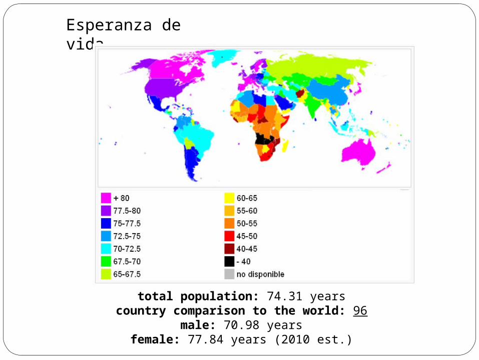
Esperanza de vida

total population: 74.31 yearscountry comparison to the world: 96

male: 70.98 yearsfemale: 77.84 years (2010 est.)