population forecasts for goomalling (s) 2006 to 2026s).pdfpopulation forecasts for goomalling (s)...
TRANSCRIPT

February 2012
Western Australia TomorrowPopulation Report No. 7, 2006 to 2026
Forecast Profile
Goomalling (S)Local Government Area

Population Report No. 7
Western Australia Tomorrow
Forecast Profile for the Goomalling (S)
Local Government Area
Published by theWestern Australian Planning Commission140 William StreetPerth, Western Australia 6000
Authors: Tom Mulholland and Anna Piscicelli
Disclaimer: Any representation, statement opinion or advice ex-pressed or implied in this publication is made in good faith and onthe basis that the government, its employees and agents are notliable for any damage or loss whatsoever which may occur as a re-sult of action taken or not taken, as the case may be, in respect ofany representation. statement opinion or advice, referred to herein.Professional advice should be obtained before applying the infor-mation contained in this document to particular circumstances.

Foreword
Western Australia Tomorrow is a set of forecasts1 based on trendssince the 1980s. The forecasts represent the best estimate of futurepopulation size if trends in fertility, mortality and migration con-tinue. They use the latest information about changes in trends. Insome cases these have occurred since the 2006 base year.
Trend forecasts are used in a number of ways. One of them is toidentify those futures which we wish to build upon and some thatwe would rather avoid. As a result government has adopted plansand strategies that are expected to change future trends. These in-clude Directions 2031 and Beyond, Pilbara Cities and Supertowns.Each of the plans and strategies has included a forecast of futurepopulation.
The forecasts within these plans and strategies differ from WA To-morrow in a number of ways. In some cases, such as Directions2031, the aggregate forecast has been consistent with WA Tomor-row. The emphasis in this plan is on meeting the requirement tofind room for future population growth while maintaining local en-vironments and valued quality of life. In other cases the forecastsrepresent an aspirational target which is seen as beneficial for thecommunities involved. The emphasis may not be on the forecastbut rather on what changes may be needed to change future pop-ulation. As a result the forecast is about direction and not theultimate size of population.
Future WA Tomorrow forecasts will incorporate the changes achievedthrough these plans and strategies. Sometimes it will be easy toknow how to incorporate the different views of the future. Readerswill need to fully understand what a particular plan or strategy istrying to achieve and make an assessment on the relevance of theplan or strategy.

Population forecasts for Goomalling (S) 2006 to 2026Overview
This population forecast is one of a set offorecasts for each Local Government Area inWestern Australia.
These forecasts have been prepared using10 0002 slightly different simulations. Thesimulations emulate the variability that isshown in past data. The simulations havebeen sorted by the size of population. They
have been broken into five bands, each with2 000 simulations. We have published the me-dian value of each band to give 5 forecasts.
Band A contains the lowest simulations.Band E has the highest simulations. Theforecast for Band C is also the median valuefor all forecasts as it is the middle band. TheBand C forecast is comparable with the pre-vious WA Tomorrow (2005) publication.
Figure 1: Forecast of total population
When assessing the probability of a fore-cast for a single region, users typically takeeach forecast to be independent.3 Past fore-casts have shown that there will be individualshires where the top of the range is easily met.The hard part is working out if Goomallingwill be a region that does not follow the trend.
In addition to past instability, all levels ofgovernment have the task of changing trendsthrough planning processes. Users should beaware of such initiatives and the impact that
they may have in the future. In some casesit may help to use any population scenariosthat are included with such projects.
Population Change
Figure 1 shows each of the bands within theforecast. The bands have been coloured4 andthe median value of each band as at 2026 hasbeen printed on the chart.
WA Tomorrow Population Report No. 7 1 Forecast Profile

Population forecasts for Goomalling (S) 2006 to 2026
The range of these forecasts suggest thatusers need to be careful when making de-cisions based on these forecasts. There isa signifcant variation between Band A andBand E that should be taken into account.
One way of looking at growth is to calculatethe average annual growth rate or AAGR.The AAGR is the constant rate of changethat is required to reach the size of popu-lation in a particular year. It is expectedthat there will be very significant populationgrowth in Goomalling. The average annualgrowth rate (AAGR) for Band C is 1.5%.This compares with a lowest change rate of
0.5% and a high of 2.3%. Migration playsan increasing role between Bands A and E.The number of births is significantly higherthan deaths. Births are also a more impor-tant component than net migration.
Table 2 shows the range of AAGRs for 20, 15and 10 years. To put these figures in contextthe rates have been compared with the Aus-tralian AAGRs prior to the recent studentinduced5 record growth rates. The Gooma-lling AAGRs are higher than the Australianexperience. By WA standards they can beconsidered to be good growth.
Figure 2: Demographic Accounts
Demographic Accounts
These forecasts have been prepared using acohort component model that includes infor-mation about migration flows in and out ofregions within Australia, net migration intoAustralia, births and deaths.
A waterfall chart (Figure 2) gives a visuali-sation of the cumulative effect of each com-ponent. Within each band the componentshave been ordered by the absolute size of theirimpact. The largest impacts are shown last.The cumulative effect of all components isequal to population change over the 20 yearperiod. The cumulative values6 are printed in
Forecast Profile 2 WA Tomorrow Population Report No. 7

Population forecasts for Goomalling (S) 2006 to 2026
red alongside the last component. The bandsare ordered so that the lowest band is on theleft and the highest is on the right. A dashedline indicates no population change. This al-lows the user to see the overall balance of thecomponents.
A feature of these forecasts is an increase inthe assumptions for fertility and overseas mi-gration into Australia. The change in fertilityrates between those used here and the onesused in the 2005 edition of WA Tomorrow is
very large. Instead of a reduction in fertil-ity, this forecast continues the current highrates of fertility for the horizon of the fore-cast. This means that births are playing amore significant role in population change,than they have previously.
The main component changed from births forBand A, to intrastate migration for Band E.As expected the birth and death compo-nents were the two most stable aspects of themodel.
Figure 3: Boxplots of demographic components
An alternative way at looking at the compo-nents is by the use of boxplots. These visual-isations allow the user to see the distributionof values in each band.
The dark-line in the centre of the boxplot isthe average (median) value of that band. 50%of the values are within the box. The whiskersattached to the box have a range that is 1.5times that of the mean to box edge. Finallyoutliers are shown as solid dots.
The boxplots show the structured way inwhich the demographic components changeeach other. There are distinct differences be-tween each of the bands. Close examinationof a single band shows that the range of val-ues used can be quite large.
Age and Sex Structure
Changes have been made in this forecast to
WA Tomorrow Population Report No. 7 3 Forecast Profile

Population forecasts for Goomalling (S) 2006 to 2026
improve the accuracy of the age and sexstructure. A detailed analysis of past fore-casts suggested that the difference betweenthe forecast and what occurred was substan-tial. Figure 4 gives a visualisation of the dy-namics of the age structure throughout theforecast. The figure is split with both thetop and bottom parts sharing the same x axis(5 year age groups.)
The top part overlays the ranges (all bands)for each age group as a polygon. There isa polygon for each census year from 2006 to
2026. Each polygon has been hatched andcoloured. Cross hatching indicates the over-lap between census years. The bottom partshows the ranges (all bands) of the AAGR foreach age group. If the bottom chart is rela-tively flat it indicates that all age groups arechanging at the same rate. In this case theranges will all share the same shape. That ispeaks and troughs will all remain in the sameage. If AAGRs have a high rate of changethen the top chart will spread out revealingthe population increase.
Figure 4: Age structure for 2006, 2011, 2016, 2021 and 2026
If the AAGRs are not flat they indicate thatsome age groups are changing faster than oth-ers. This is nearly always the case for theolder age groups. This part of the chart en-ables the user to gauge how individual agegroups are changing in comparison to eachother.
During the period of these forecasts the agestructure remains familiar. There is quite a
lot of overplotting on these charts.
The AAGRs for young people (aged 0 to 19)centres around 1.8%. Those of working age(20 to 64) have a rate of about 0.8%. Olderpeople have a rate closer to 4.2%.
Analysis of the output from this model showsthe forecasts do not exhibit the universal agecreep7 that was a prominent feature of previ-
Forecast Profile 4 WA Tomorrow Population Report No. 7

Population forecasts for Goomalling (S) 2006 to 2026
ous forecasts. This was most noticeable in ar-eas where there were strong migration trendsthat suggested a stable age and sex struc-ture. These were typically associated withmining employment or attendance at an edu-cational institution. In past forecasts an ad-hoc adjustment was made using past trendsof changes in the structures. In line withacademic work8 the introduction of migrationflows appears to have resulted in improved es-timates of age and sex.
Assumptions used in the model for
Goomalling (S)
The assumptions for each area have been cre-ated using both local and State data. It hasbeen shown that local forecasts of populationare improved by adjusting each sub-region sothat the sum of the components results in thesame outcome as the State estimate.
Details of the assumptions used at a Statelevel are included in the summary publica-tions.
Mortality assumptions in Goomalling (S) arederived for both the Indigenous population aswell as the non-Indigenous population. Whilethere is no way to accurately determine thelocal mortality rates for Indigenous people,it is well known that there are very signifi-cant differences between the two groups. Theforecasts do this because in areas with sub-stantial Indigenous populations, even a crudeestimate of Indigenous mortality can signifi-cantly improve the forecast.
Figure 5 is for the total population and takesaccount of all of the adjustments made in theforecast process. It is usual to transform therate by applying a log function. This enablesthe reader to see the subtle changes that arehappening.
Figure 5: Age specific mortality rates for the years 2011 to 2012, 2015 to 2016 and 2025 to2026
WA Tomorrow Population Report No. 7 5 Forecast Profile

Population forecasts for Goomalling (S) 2006 to 2026
Figure 6: Age specific fertility rates for the years 2011 to 2012, 2015 to 2016 and 2025 to2026
The use of a State-wide assumption was madeafter looking at the spatial variations in mor-tality. A recent Australian Bureau of Statis-tics publication9 produced an article lookingat remoteness areas and found that there wasa difference between remote and non remoteareas. There seems to be a similarity betweenthis finding and the one used in this publi-cation. That is remoteness is also associatedwith higher proportions of Indigenous people.
This topic is part of ongoing discussion withthe Australian Bureau of Statistics to im-prove the quality of Indigenous statistics. Itdoes not appear that there is an obvious wayto spatially vary mortality rates at the mo-ment.
Local fertility assumptions were made byidentifying regions that had a similar fertil-ity pattern. For example the outer areas ofPerth have higher levels and a younger peakof age specific rates than the inner areas ofPerth. Likewise urban centres in the coun-try had lower rates and an older peak in agespecific rates than other country areas.
The rates for these groupings were used forall areas within the grouping. The variationin rates between individual areas is incorpo-rated in the uncertainty shown in Figure 6.
A single assumption was used for the Indige-nous mothers. The net effect of both assump-tions have been combined in Figure 6.
Forecast Profile 6 WA Tomorrow Population Report No. 7

Population forecasts for Goomalling (S) 2006 to 2026
Figure 7: Age specific migration rates for the years 2006 to 2026
Rates for the three migration types used inthe model are shown in Figure 7. Theseare net migration rates. They are helpfulin understanding the change in populationsize. However, they also hide most of the mi-gration that actually occurs. Approximately10% of the total population will have movedto Goomalling from elsewhere in WA, eachyear. Interstate migrants add another 1%.The figure for net overseas migrants is notcalculated using flows. Therefore the inwardcomponent is unavailable. However as withthe other migration flows it is probably muchlarger than the net migration estimate.
Estimates of overseas migration have beenmade using linear regression. From this con-fidence intervals have been used to estimatethe levels of uncertainty. However past levelsof overseas migration have been influenced bychanges to government policy. These changeshave often been sudden and dramatic. Thistype of uncertainty is not included in theseforecasts.
The estimates for overseas migration mayincorrectly contain movements within Aus-tralia. This is because there is no direct wayof estimating who has moved overseas fromGoomalling. It could be that people who haveleft, failed to identify Goomalling as their pre-vious address on the Census form. This willhave most impact for groups, such as youngmales, who tend to either be missed or fail toanswer questions on the Census form.
WA Tomorrow Population Report No. 7 7 Forecast Profile

Population forecasts for Goomalling (S) 2006 to 2026
Notes
1As with the previous set of projectionsthe terms forecast and projection have thesame meaning within this document.
2 While this may seem like a large num-ber of runs, it is in fact less than would berequired to be able to say with any degreeof certainty that an alternative run of 10 000would not give significantly different figures.
For example, if we tried to select a combi-nation of factors that ensured each year hadfive runs that covered the possibilities be-tween low and high we would need 95 tril-lion unique runs to cover all possible permu-tations.
In the first year there would be five pos-sibilities. In the second year each of the fiveoptions have 5 more options. This is nor-mally shown as 52 or 5 to the power of 2 whichequals 25. The next year we have 53 or 5 tothe power of 3 which equals 125. To do the20 years in the forecast we need 521 or 95 367431 640 625 or 95 trillion.
Running this many simulations is notpossible. Our 10 000 simulations represent asample which we can use as representative ofthe minimum of 95 trillion possibilities. Us-ing a sample size calculator the best we canexpect of the mean of all simulations is thatthey are within 1% plus or minus and we areabout 95% confident about that. The use of1 000 runs changes that to 3%. The realityis that both figures are much larger as thereis no way that we only need 476 trillion sim-ulations. Most of them will be duplicates. Itseems likely that we are probably within theball park and not much else.
3 This forecast is part of a series. All ofthem are related to each other. Some will behigher and some will be lower. It is unrealistic
to expect them to all be average. For exam-ple if you throw six dice, you expect that oneof the dice will roll a six quite quickly. Indeedthere is a 66% chance that it will be thrownin the first 6 rolls and a 90% probability thata five or six will be thrown.
4 These colours have been selected so thatpeople with some of the more common typesof colour blindness can distinguish the differ-ences.
5 Recent population growth in Australiahas been connected with changes to the wayin which the population is counted. Thechange mainly relates to people who are inAustralia for longer than 1 year, but donot have permanent residence status, such asoverseas students. For a while a boom in vo-cational education encouraged high levels ofstudents hoping to gain permanent residencein Australia. Changes to migration processesin 2010 appear to have reduced the numbersof students.
6Since the forecasts are sorted in order torank the runs for each year, the median val-ues of the demographic components are notrequired to add to the size of the total popula-tion. For smaller areas the differences may belarge enough to notice. However the overallpattern will be correct. Using an individualrun could produce a run that was not rep-resentative of the change from band to band,although the sum of the components could beguaranteed to total correctly.
7 Age creep is the way the existing agestructure appears to age in place. That is af-ter 5 years a peak that was at age 20 nowpeaks at age 25, suggesting that the popula-tion is stable and therefore the 20 year oldsare most likely the same 15 year olds.
8Isserman, A. M. (1993). The RightPeople, the Right Rates Making PopulationEstimates and Forecasts with an InterregionalCohort-Component Model. Journal of the
Forecast Profile 8 WA Tomorrow Population Report No. 7
Population forecasts for Goomalling (S) 2006 to 2026
American Planning Association 59(1): 45-64.
Kupiszewski, M. and P. Rees(1999). Lessons for the projection of inter-nal migration from studies in ten Europeancountries. Statistical Journal of the UnitedNations 16 281 - 295.
Rees, P. (1985). Developments in themodelling of spatial populations. PopulationStructures and Models: Development in spa-tial demography. R. Woods and P. Rees.London, Allen & Unwin: 97-124.
Rogers, A. (1975). Shrinking Large-
Scale Population Projection Models by Ag-gregation and decomposition. Laxenburg,IIASA. p. 60.
Wilson, T. and M. Bell (2004). Com-parative empirical evaluations of internal mi-gration models in subnational population pro-jections. Journal of Population Research21(2): 127-160.
9 ABS (2011). Deaths, Aus-tralia. 2010, 3302.0. Canberra, Aus-tralian Bureau of Statistics. Website:www.abs.gov.au/ausstats/[email protected]/mf/3302.0
WA Tomorrow Population Report No. 7 9 Forecast Profile

Population forecasts for Goomalling (S) 2006 to 2026
Table 1: Population Forecasts by Bands 2006 to 2026
A B C D E2006 980 980 980 990 9902007 960 980 1 000 1 000 1 0002008 960 990 1 000 1 000 1 1002009 940 1 000 1 000 1 100 1 1002010 940 1 000 1 100 1 100 1 2002011 930 1 000 1 100 1 100 1 2002012 930 1 000 1 100 1 200 1 2002013 940 1 000 1 100 1 200 1 3002014 950 1 100 1 100 1 200 1 3002015 960 1 100 1 100 1 200 1 3002016 970 1 100 1 200 1 200 1 3002017 980 1 100 1 200 1 300 1 4002018 990 1 100 1 200 1 300 1 4002019 1 000 1 100 1 200 1 300 1 4002020 1 000 1 100 1 200 1 300 1 4002021 1 000 1 200 1 200 1 300 1 5002022 1 000 1 200 1 300 1 300 1 5002023 1 000 1 200 1 300 1 400 1 5002024 1 100 1 200 1 300 1 400 1 5002025 1 100 1 200 1 300 1 400 1 5002026 1 100 1 200 1 300 1 400 1 600
Table 2: AAGRs and Australian Ratio by Bands, 2026, 2021 and 2016
AAGR RatioA B C D E A B C D E
2026 0.5 1.1 1.5 1.8 2.3 0.4 0.9 1.2 1.5 1.92021 0.3 1.1 1.6 2.0 2.6 0.2 0.9 1.3 1.7 2.22016 −0.1 1.0 1.7 2.3 3.1 −0.1 0.8 1.4 1.9 2.6
Forecast Profile 10 WA Tomorrow Population Report No. 7

Population forecasts for Goomalling (S) 2006 to 2026
Table 3: Population Forecasts by Age and Bands 2011
A B C D E0 to 4 70 75 80 85 905 to 9 65 75 75 80 85
10 to 14 70 75 80 80 8515 to 19 35 40 45 45 5020 to 24 35 45 50 55 6025 to 29 60 70 80 90 10030 to 34 60 70 80 85 9535 to 39 55 65 70 75 8540 to 44 50 60 65 65 7545 to 49 55 60 65 65 7050 to 54 70 75 75 75 8055 to 59 75 80 80 85 8560 to 64 70 70 75 75 7565 to 69 45 50 50 50 5070 to 74 45 45 45 50 5075 to 79 30 30 30 30 3080 to 84 20 20 20 20 20
85 and over 15 15 15 15 15
Table 4: Population Forecasts by Age and Bands 2016
A B C D E0 to 4 75 85 95 100 1105 to 9 80 90 95 100 110
10 to 14 65 70 75 80 9015 to 19 40 45 45 50 5520 to 24 35 40 45 50 5525 to 29 60 75 80 90 10030 to 34 80 95 110 110 13035 to 39 60 75 80 90 10040 to 44 45 55 60 65 7545 to 49 40 50 55 60 7050 to 54 55 60 65 70 7555 to 59 75 80 85 85 9560 to 64 70 75 80 80 8565 to 69 55 60 60 65 6570 to 74 45 45 45 50 5075 to 79 40 40 40 45 4580 to 84 20 20 20 25 25
85 and over 20 20 20 20 20
WA Tomorrow Population Report No. 7 11 Forecast Profile
Population forecasts for Goomalling (S) 2006 to 2026
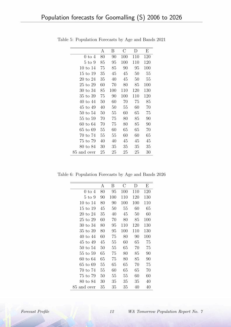
Table 5: Population Forecasts by Age and Bands 2021
A B C D E0 to 4 80 90 100 110 1205 to 9 85 95 100 110 120
10 to 14 75 85 90 95 10015 to 19 35 45 45 50 5520 to 24 35 40 45 50 5525 to 29 60 70 80 85 10030 to 34 85 100 110 120 13035 to 39 75 90 100 110 12040 to 44 50 60 70 75 8545 to 49 40 50 55 60 7050 to 54 50 55 60 65 7555 to 59 70 75 80 85 9060 to 64 70 75 80 85 9065 to 69 55 60 65 65 7070 to 74 55 55 60 60 6575 to 79 40 40 45 45 4580 to 84 30 35 35 35 35
85 and over 25 25 25 25 30
Table 6: Population Forecasts by Age and Bands 2026
A B C D E0 to 4 80 95 100 110 1205 to 9 90 100 110 120 130
10 to 14 80 90 100 100 11015 to 19 45 50 55 60 6520 to 24 35 40 45 50 6025 to 29 60 70 80 85 10030 to 34 80 95 110 120 13035 to 39 80 95 100 110 13040 to 44 60 75 80 90 10045 to 49 45 55 60 65 7550 to 54 50 55 65 70 7555 to 59 65 75 80 85 9060 to 64 65 75 80 85 9065 to 69 55 65 65 70 7570 to 74 55 60 65 65 7075 to 79 50 55 55 60 6080 to 84 30 35 35 35 40
85 and over 35 35 35 40 40
Forecast Profile 12 WA Tomorrow Population Report No. 7

Population forecasts for Goomalling (S) 2006 to 2026
Table 7: Boxplot Values for Top 20%
Births Deaths Interstate Intrastate OverseasLower Whisker 400 -200 100 -800 200
Box Bottom 400 -200 200 -600 400Median 400 -200 200 -500 400
Top Box 400 -200 300 -400 500Upper Whisker 500 -200 400 -200 700
Table 8: Boxplot Values for 60-80%
Births Deaths Interstate Intrastate OverseasLower Whisker 400 -200 0 -500 100
Box Bottom 400 -200 100 -300 200Median 400 -200 200 -300 200
Top Box 400 -200 200 -200 300Upper Whisker 400 -100 300 0 400
Table 9: Boxplot Values for Middle 20%
Births Deaths Interstate Intrastate OverseasLower Whisker 300 -200 0 -400 0
Box Bottom 400 -200 100 -200 100Median 400 -200 100 -100 100
Top Box 400 -100 100 -100 200Upper Whisker 400 -100 200 100 300
Table 10: Boxplot Values for Top 20-40%
Births Deaths Interstate Intrastate OverseasLower Whisker 300 -200 -100 -200 -200
Box Bottom 300 -100 0 -100 -100Median 300 -100 100 0 0
Top Box 300 -100 100 0 0Upper Whisker 400 -100 200 200 200
WA Tomorrow Population Report No. 7 13 Forecast Profile

Population forecasts for Goomalling (S) 2006 to 2026
Table 11: Boxplot Values for Bottom 20%
Births Deaths Interstate Intrastate OverseasLower Whisker 200 -200 -100 -100 -600
Box Bottom 300 -100 0 100 -400Median 300 -100 0 200 -300
Top Box 300 -100 0 300 -200Upper Whisker 300 -100 100 500 0
Forecast Profile 14 WA Tomorrow Population Report No. 7