polytechnic university of bari - orbi: home chiara... · the polytechnic university of bari...
TRANSCRIPT
POLYTECHNIC UNIVERSITY OF BARI
INTERPOLYTECHNIC DOCTORAL SCHOOL
Doctoral Program in
Environmental and Territorial Safety and Control (ETSC)
Final Dissertation
Development and validation of analytical methods based
on GC-MS/MS Triple Quadrupole instrument for the
analysis of POPs in food and feed matrices
Chiara Calaprice
Supervisors
Prof. Pietro Mastrorilli (Poliba)
Prof. Carlo Zambonin (Uniba)
Dott.ssa Cosima Damiana Calvano (Uniba)
Prof. Jean François Focant (ULg)
Co-ordinator of the
Research Doctorate Course
Prof. Michele Mossa (Poliba)
4th April 2016


PhD in joint agreement between
The Polytechnic University of Bari (Poliba) and the University of Liège (ULg)
With the scientific support of the University of Bari (Uniba)


POLITECNICO DI BARI
SCUOLA INTERPOLITECNICA DI DOTTORATO
Area Scientifica Protezione e Controllo di Ambiente e Territorio
(ETSC)
Tesi Finale
Sviluppo e validazione di metodi analitici basati sulla
spettrometria di massa a Triplo Quadrupolo per l’analisi
di composti organici persistenti (POPs) in prodotti per
l’alimentazione umana e animale
Chiara Calaprice
Supervisori
Prof. Pietro Mastrorilli (Poliba)
Prof. Carlo Zambonin (Uniba)
Dott.ssa Cosima Damiana Calvano (Uniba)
Prof. Jean François Focant (ULg)
Co-ordinatore della Scuola di Dot-
torato
Prof. Michele Mossa (Poliba)
4 Aprile 2016


To my beloved grandparents

i
EXTENDED ABSTRACT (eng)
This thesis focused on the development and validation of analytical methods for the de-
tection and quantification of Persistent Organic Pollutants (POPs) in biological matrices,
namely food and feed samples. POPs are a group of chemical compounds listed after the
Stockholm Convention in 2001, with demonstrated toxicity and dangerousness for envi-
ronment, animals and humans.
In this work of thesis, special attention was reserved to some selected POPs: poly-
chlorodibenzo-p-dioxins (PCDDs), polychlorodibenzofurans (PCDFs), usually referred to
as “dioxins”, and polychlorinated biphenyls (PCBs), as there is a big concern about these
contaminants in Taranto, a city in the Southern Italy very close to Bari, my home town.
Taranto, indeed, is characterized by a large industrial area with a steel mill, several incin-
erators and a refinery in few kilometre radius (Di Leo et al., 2014). This work has been
done in collaboration with the University of Liège (Belgium) where a consolidated exper-
tise in the field of POP measurements was available, especially in terms of dioxin analy-
ses.
In Chapter 1 the main steps, from sample preparation to data elaboration, of a validated
confirmatory method for dioxin and PCB detection in food and feed using gas chromatog-
raphy coupled to tandem mass spectrometry Triple Quad instrument (GC-MS/MS Triple
Quad) have been described. This method was developed at the University of Liège in the
framework of the last updates of the EU Regulation that in 2014 allowed confirmatory
quantitative analysis of dioxins with Triple Quad. This method was the starting point of
this work of thesis, because it was used for all dioxin and PCB quantifications. In Chapter
2 and chapter 3 alternative clean-up approaches for dioxin analysis in fatty food matrices
have been developed using different automated systems. These works have been done
in the framework of solvent and time saving for high throughput analytical methods in di-
oxin analysis. In chapter 2, an already existing automated system, DEXTechTM from
LCTech GmbH (LCTech GmbH, Bahnweg 41, 84405 Dorfen, Germany) was used for
sample clean-up, but a completely new clean-up approach was developed with this. GC-
MS/MS Triple Quad instrument, as well as Magnetic Sector High Resolution Mass Spec-
trometry (HRMS) instrument were employed for final quantification, to demonstrate the

ii
suitability of our newly developed clean-up approaches whatever the instrumental detec-
tion. In Chapter 3 PowerPrepTM automated system from Fluid Management System (FMS
Inc., 580 Pleasant Street, Watertown, MA 02472, USA) was used and our routine sample
clean-up approach was modified in order to enhance the efficiency and to reduce cost
and solvent consumption of the analysis. In Chapter 4 the main method for dioxin analysis
was adapted for the integration of Dechloranes in the list of the analytes targeted in the
regular control for dioxins in food and feed. Dechloranes are a family of 6 organo-
chlorinated compounds with structure similar to Mirex, also called Dechlorane, a POP
listed in the Stockholm convention. Dechloranes have been found in human blood of peo-
ple from Europe (Brasseur et al., 2014) and in this work an analytical method for
Dechlorane detection was developed and validated to investigate food as a possible route
of exposure for humans in Europe, where no production plant has been identified so far.
The analytical method was used to analyse 88 food and feed real sample and to give an
idea of Dechlorane daily dietary intake.
Dioxins, PCBs, GC-MS/MS Triple Quadrupole, method validation,
Dechloranes

iii
EXTENDED ABSTRACT (ita)
Questo lavoro di tesi è stato incentrato sullo sviluppo e la validazione di metodi analitici
per la rivelazione e la quantificazione di composti organici persistenti (Persistent Organic
Pollutants, POPs) in campioni biologici, in particolare campioni di cibo per l’alimentazione
umana e animale. Il termine “POPs” comprende un gruppo di composti chimici, elencati
durante la Convenzione di Stoccolma nel 2001, la cui tossictà e pericolosità per l’uomo,
gli animali e l’ambiente sono dimostrate. In questo lavoro di tesi è stata dedicata partico-
lare attenzione ad alcuni POPs, come diossine (polychlorodibenzo-p-dioxins, PCDDs), fu-
rani (polychlorodibenzofurans, PCDFs) e bifenili policlorurati (polychlorinated biphenyls,
PCBs), poichè questi composti suscitano molta preoccupazione per la salute umana nella
città di Taranto, una città a Sud dell’Italia, situata vicino a Bari, la mia città natale. Taran-
to, infatti, è caratterizzata dalla presenza di una acciaieria, vari inceneritori e una raffineri-
a, concentrate nell’area industriale della città e non molto distanti fra loro. Questo lavoro
di tesi è stato svolto in collaborazione con l’Università di Liegi (Belgio), che possiede e-
sperienza decennale ed internazione nell’ambito dell’analisi di diossine.
Nel Capitolo 1 di questo lavoro di tesi sono descritti i passaggi principali dell’analisi delle
diossine, dalla preparazione del campione all’analisi strumentale utilizzando la tecnica di
gas cromatografia accoppiata alla spettrometria di massa con analizztore a Triplo Qua-
drupolo (GC-MS/MS Triple Quad). Questo metodo analitico, che è stata la base di questo
lavoro di tesi, è stato sviluppato all’Università di Liegi nel quadro degli ultimi aggiorna-
menti della Regolamentazione Europea in materia di diossine, che nel 2014 ha accettato
l’utilizzo del Triplo Quadrupolo per l’analisi quantitativa di questi composti. La maggior
parte delle analisi descritte in questo lavoro sono state effettuate con il Triplo Quadrupolo
sulla base del suddetto metodo analitico. Nei Capitoli 2 e 3 sono descritti degli approcci
alternativi per il clean-up del campione, utilizzando sistemi automatici. In particolare nel
Capitolo 2, per il clean-up del campione, è stato utilizzato il DEXTechTM della compagnia
tedesca LCTech (LCTech GmbH, Bahnweg 41, 84405 Dorfen, Germany), per il quale è
stato sviluppato un approccio completamente nuovo per il suo utilizzo. Le successive
analisi quantitative sono state fatte con il Triplo Quadrupolo e con il Settore Magnetico,
per dimostrare la validità dell’approccio proposto a prescindere dalla tecnica impiegata
iv
per l’analisi strumentale finale. Nel Capitolo 3, per il clean-up del campione, è stato utiliz-
zato il PowerPrepTM, prodotto dalla compagnia americana FMS (FMS Inc., 580 Pleasant
Street, Watertown, MA 02472, USA); il metodo di clean-up utilizzato routinariamente nel
nostro laboratorio a Liegi, è stato opportunamente midificato con l’obiettivo di ridurre i
tempi e i costi della preparativa del campione. Infine, l’analisi strumentale è stata effettua-
ta con il Settore Magnetico. Infine, nel Capitolo 4, il metodo analitico per l’analisi di dios-
sine, è stato modificato per consentire l’analisi simultanea di diossine e di Declorani, che
sono una famiglia di composti potenzialmente pericolosi. Il primo di questi composti è sta-
to il mirex, noto anche come Declorano, che è inserito nella lista dei POPs della Conven-
zione di Stoccolma. I Declorani sono stati trovati in campioni di sangue umano in soggetti
provenienti dalla Francia. In questo lavoro di tesi, è stato sviluppato e validato un metodo
analitico per la rivelazione di questi composti in campioni destinati all’alimentazione uma-
na ed animale, per capire se la catena alimentare rappresenta una possibile via di espo-
sizione a questi composti in Europa, dove non è stato identificato alcun impianto di pro-
duzione di Declorani. Il metodo analitico sviluppato è stato applicato a 88 campioni reali di
varie matrici alimentari e un apporto giornaliero di Declorani è stato stimato sulla base
delle abitudini alimentari della popolazione belga.
Diossine, PCBs, GC-MS/MS Triple Quadrupole, validazione di metodi
analitici, Declorani

v
LIST OF GENERAL ABBREVIATIONS
ABN Acid Basic Neutral silica column
ARRF Average Relative Response Factor
AhR Aryl hydrocarbon Receptor
ASE Accelerated Solvent Extraction
ATSDR Agency for Toxic Substances and Diseases Registry
CART Centre for Analytical Research and Technology
CONTAM Panel of EFSA on Contaminants in the Food Chain
co-PCBs Coplanar PCBs (#77, 81, 126, 169)
DCM Dichloromethane
DL Detection limit
DL-PCBs Dioxin-like PCBs
DoE Design of Experiment
DP Dechlorane Plus
EC European Commission
EFSA European Food Safety Authority
EI Electron Ionization
EPA Environmental Protection Agency
EURL European Reference Laboratories
fanti Ratio between the concentration of DPanti and DPsyn isomers
FCD Face Centered Design
FFD Full Factorial Design
GC-MS/MS Gas chromatography – tandem mass spectrometry
HC High Capacity
HCCPD Hexachlorocyclopentadiene
HRMS High Resolution Mass Spectrometry

vi
ID Isotope Dilution
iLOQ Instrumental Limit of Quantitation
I-PCBs Indicator PCBs (# 28, 52, 101, 138, 153, 180)
ISTD Internal Standard, often labelled
lb Lower bound (approach of reporting final result in dioxin
analysis)
LOQ Limit of Quantitation
LVI Large Volume Injection
LRMS Low Resolution Mass Spectrometry
ML Maximum residual Level
MO-PCBs Mono-ortho PCBs (#105, 114, 118, 123, 156, 157, 167, 189)
MRM Multiple Reaction Monitoring
NDL-PCBs Non-dioxin like PCBs
NRL National Reference Laboratory
PBMS Performance-based Measurement System
PCBs Polychlorinated biphenyl
PCDDs Polychlorinated dibenzo-p-dioxins
PCDFs polychlorinated dibenzofurans
PCP Pentachloro phenol
PLE Pressurised Liquid Extraction
ppb Part-per-billion (10-9)
ppm Part-per-million (10-6)
ppq Part-per-quadrillion (10-15)
ppt Part-per-trillion (10-12)
PTV Programmable Temperature Vaporization
QC Quality Control
QCE Quality Control egg
QCG Quality Control fat
vii
QCL Quality Control milk
QIST Quadrupole Ion Storage tandem-in-time mass spectrometer
QQQ Triple Quadrupole
RRF Relative Response Factor
S/N Signal to Noise ratio
SIM Single Ion Monitoring
ST ROU Standard routine
TCDD Tetrachloro dibenzo-p-dioxin
TEF Toxic Equivalent Factor
TEQ Toxic equivalents
ub Upper bound (approach of reporting final result in dioxin
analysis)
VF Vent Flow
VP Vent Pressure
WHO World Health Organization

viii
ix
INDEX
INTRODUCTION ............................................................................................................................................. 1
AIM OF THIS WORK .......................................................................................................................... 3 SCIENTIFIC CONTEXT OF THE RESEARCH ABOUT DIOXINS AND PCBS ............................................................... 5 1. DIOXIN AND PCB STRUCTURE RELATED TOXICITY ........................................................................ 7 2. DIOXIN SOURCES AND ENVIRONNEMENTAL CONTAMINATION ......................................................... 11
2.1. Primary sources ....................................................................................................... 11 2.2. Secondary sources .................................................................................................. 13 2.3. Fate and transport .................................................................................................... 14
3. PCB SOURCES AND FATE ...................................................................................................... 15 3.1. Industrial production ................................................................................................. 15 3.2. Secondary sources .................................................................................................. 17 3.3. Fate and transport .................................................................................................... 19
4. RISK ASSESSMENT, TOXIC EQUIVALENT FACTOR (TEF) AND EUROPEAN REGULATION ......................... 19 SCIENTIFIC CONTEXT OF THE RESEARCH ABOUT DECHLORANES ............................................................. 24 BIBLIOGRAPHY ............................................................................................................................. 26
CHAPTER I
DESCRIPTION OF A VALIDATED GAS CHROMATOGRAPHY-TRIPLE QUADRUPOLE MASS SPECTROMETRY METHOD FOR
CONFIRMATORY ANALYSIS OF DIOXINS AND DIOXIN-LIKE POLYCHLOROBIPHENYLS IN FEED. .................................. 29
1. INTRODUCTION .................................................................................................................... 29 2. GENERAL MAIN STEPS OF ANALYTICAL METHODS FOR DIOXIN AND PCB ANALYSIS ............................. 31 3. CHEMICALS AND CONSUMABLES ............................................................................................. 33 4. SAMPLE PREPARATION FOR VEGETABLE OIL IN OUR LABORATORY .................................................. 37 5. GC-MS/MS TRIPLE QUAD INSTRUMENTAL SETUP ...................................................................... 38 6. MAIN FEATURES OF THE VALIDATED INSTRUMENTAL METHOD WITH GC-MS/MS TRIPLE QUAD
INSTRUMENT ................................................................................................................................ 39 6.1. Validation criteria in the EU Regulation....................................................................... 40 6.2. MRM transitions ....................................................................................................... 43 6.3. Calibration range and retention time .......................................................................... 45 6.4. Limit of Quantitation (LOQ) and detectable quantity ..................................................... 47 6.5. Selectivity ................................................................................................................ 51 6.6. Accuracy: trueness and precision .............................................................................. 52
CHAPTER II
DEVELOPMENT OF A NEW DIOXIN/PCB CLEAN-UP AND FRACTIONATION PROCEDUREFOR AN EXISTING AUTOMATED
SYSTEM ........................................................................................................................................................... 57
1. INTRODUCTION .................................................................................................................... 57 2. MATERIALS AND METHODS..................................................................................................... 59
2.1. Chemicals and consumables ..................................................................................... 59
x
2.2. Sample preparation .................................................................................................. 60 2.2.1. DEXTechTM system for sample clean-up..................................................................... 61
2.3. Instrumental quantification ........................................................................................ 64 3. RESULTS AND DISCUSSION .................................................................................................... 65
3.1. Classic clean-up scheme .......................................................................................... 65 3.2. Alternative approach scheme .................................................................................... 67
3.2.1. Conditioning step ..................................................................................................... 70 3.2.2. Silica column elution profile ....................................................................................... 70 3.2.3. Alumina column ....................................................................................................... 72 3.2.4. Carbon column ........................................................................................................ 76
3.2.4.1.Clarge - Carbopack C:celite elution profile ........................................................... 76 3.2.4.2.Csmall – Norit:celite elution profile ...................................................................... 78
3.3. QC samples ............................................................................................................ 81 3.3.1. QCG ....................................................................................................................... 82 3.3.2. QCE and QCL ......................................................................................................... 83
4. CONCLUSIONS .................................................................................................................... 85
CHAPTER III
REVISITING AN EXISTING DIOXIN/PCB CLEAN-UP AND FRACTIONATION PROCEDURE TO REDUCE SOLVENT AND TIME
CONSUMPTION ................................................................................................................................................. 89
1. INTRODUCTION .................................................................................................................... 89 2. MATERIALS AND METHOD ...................................................................................................... 89
2.1. Chemicals and consumables ..................................................................................... 89 2.2. Sample preparation .................................................................................................. 90
2.2.1. PowerPrepTM automated system for sample clean-up .................................................. 91 2.3. Instrumental quantification ........................................................................................ 92
3. RESULTS AND DISCUSSION .................................................................................................... 93 3.1. Classic sample clean-up in our laboratory................................................................... 93
3.1.1. Manual step............................................................................................................. 94 3.1.2. Automated step ....................................................................................................... 95
3.2. Alternative approaches ............................................................................................. 96 3.2.1. Samples with fat content lower than 1 g ..................................................................... 96
3.2.1.1.Short standard method ...................................................................................... 97 3.2.1.2.Fast standard method ....................................................................................... 101
3.2.2. Samples with fat content higher than 1 g ................................................................... 103 3.2.2.1.Test on feed and food samples .......................................................................... 106
3.3. Alumina sorbent features ......................................................................................... 109 4. CONCLUSIONS ................................................................................................................... 111
xi
CHAPTER IV
ULTRA-TRACE MEASUREMENT OF DECHLORANES TO INVESTIGATE FOOD AS A ROUTE OF HUMAN EXPOSURE ...... 113
1. INTRODUCTION ................................................................................................................... 113 2. DECHLORANE STRUCTURES .................................................................................................. 114 3. DECHLORANE SOURCES, ENVIRONMENTAL AND BIOLOGICAL CONTAMINATION ................................. 116 4. MATERIALS AND METHODS.................................................................................................... 116
4.1. Chemicals and consumables .................................................................................... 116 4.2. Samples ................................................................................................................. 117 4.3. Sample preparation: extraction and clean up ............................................................. 117 4.4. GC-MS/MS conditions ............................................................................................. 119
5. RESULTS AND DISCUSSION ................................................................................................... 120 5.1. Sample clean-up ..................................................................................................... 120 5.2. Experimental design for optimization of PTV parameters ............................................. 122
5.2.1. Structure of the experimental design ......................................................................... 122 5.2.2. Peak area .............................................................................................................. 124 5.2.3. Peak symmetry ....................................................................................................... 126 5.2.4. Optimum values for inlet parameters. ........................................................................ 127
5.3. Instrumental method development and validation ....................................................... 129 5.3.1. MRM transitions ...................................................................................................... 131 5.3.2. Calibration range .................................................................................................... 134 5.3.3. Limit of Quantitation (LOQ) ...................................................................................... 134 5.3.4. Selectivity ............................................................................................................... 135 5.3.5. Result reporting ...................................................................................................... 137
5.4. Dechlorane levels in food and feed matrices .............................................................. 137 5.5. Estimation of Dechlorane dietary intake ..................................................................... 142
6. CONCLUSIONS ................................................................................................................... 143
CONCLUSIONS .......................................................................................................................................... 147
ACKNOWLEDGEMENTS ........................................................................................................................... 151
CURRICULUM............................................................................................................................................153

1
INTRODUCTION
Persistent Organic Pollutants, often indicated with the acronym “POPs”, are carbon-based
chemicals addressed in the Stockholm Convention signed by 151 Countries in 2001. The
Stockholm Convention has as its objective the environmental, as well as human and biota
health protection from POPs.
Initially the list of POPs included only 12 compounds, 10 intentionally and 2 non-
intentionally produced. With time the list has been updated and new compounds showing
POP characteristics have been included. In fact POPs are considered all the chemicals
that exhibit common characteristics such as chemical and physical stability under envi-
ronmental conditions, semi-volatility, low solubility in water, and inherent toxicity. The
combination of these chemical and physical properties results in long-range transport and
in bioaccumulation. Indeed POPs are found in regions far from where they have been
used or released. Due to their lipophilicity and their environmental and metabolic persis-
tence they accumulate in the food-chain and high concentrations have been detected in
animals and humans.
In the Stockholm convention list, POPs are grouped in Annexes A, B and C (Table I.1)
based on the measure to be taken on them by parties: compounds in Annex A must be
eliminated (neither produced or used); chemical in Annex B must be restricted in the pro-
duction and use; compounds in Annex C are unintentionally produced and result as by-
products from other industrial processes, so their unintentional release must be restricted
until the complete elimination.

2
Table I.1: List of POPs decided by the Stockholm convention (Stockholm Convention official(www.pops.int/)
Annex A Annex B Annex C
Aldrin (P) DDT (P) Hexachlorobenzene (HCB) (UP)
Chlordane (P) Perfluorooctane sulfonic
acid, its salts and per-
fluorooctane sulfonyl fluo-
ride (IC)
Pentachlorobenzene (UP)
Chlordecone (P) Polychlorinated biphenyls (PCB) (IC)
Dieldrin (P) Polychlorinated dibenzo-p-dioxins
(PCDD) (UP)
Endrin (P) Polychlorinated dibenzofurans (PCDF)
(UP)
Heptachlor (P)
Hexabromobiphenyl (IC)
Hexabromocyclododecane (HBCD)
(IC)
Hexabromodiphenyl ether and
heptabromodiphenyl ether (IC)
Hexachlorobenzene (HCB) (P and
IC)
Alpha hexachlorocyclohexane (P)
Beta hexachlorocyclohexane (P)
Lindane (P)
Mirex (P)
Pentachlorobenzene (P and IC)
Polychlorinated biphenyls (PCB)
(IC)
Technical endosulfan and its re-
lated isomers (P)
Tetrabromodiphenyl ether and pen-
tabromodiphenyl ether (IC)
Toxaphene (P)
P = pesticide; IC = industrial chemical; UP = unintentional product

3
Aim of this work
This thesis focused on the development and validation of analytical methods for POP de-
tection and quantification in biological matrices, namely food and feed. Special attention
was reserved to some selected POPs: toxic PCDDs, PCDFs and PCBs, as there is a big
concern about these contaminants in Taranto (Italy), a city in the Southern Italy character-
ized by a large industrial area with a steel mill, several incinerators and a refinery (Di Leo
et al., 2014). The collaboration with the University of Liège started because of the con-
solidated expertise owned in POPs field, especially in dioxin analysis. Experimental activi-
ties described in the chapters have been carried out mainly at the University of Liège, in
collaboration with the CART (Centre for Analytical Research and Technology), which is
referred to as “our laboratory” during the following dissertation.
In Chapter 1 the main steps, from sample preparation to data elaboration, of our validated
confirmatory method for PCDD/Fs and dioxin-like (DL-) PCBs detection in food and feed
have been described. Our method is based on gas chromatography coupled to tandem
mass spectrometry Triple Quad instrument (GC-MS/MS Triple Quad) in the framework of
the last updates of the EU Regulation in this field (L'Homme et al., 2015).
In Chapter 2 alternative clean-up approaches for dioxin analysis in fatty food matrices
have been shown. These approaches were developed using an already existing auto-
mated system, DEXTechTM from LCTech GmbH (LCTech GmbH, Bahnweg 41, 84405
Dorfen, Germany), but they were based on a completely new column set in the framework
of faster, cheaper and more environmental sustainable processes. In this project instru-
mental quantification has been done mainly with GC-MS/MS Triple Quad instrument, but
also with Magnetic Sector high resolution mass spectrometry (HRMS) instrument to dem-
onstrate the suitability of the clean-up approaches whatever the instrumental detection.
In Chapter 3 alternative approaches based on our routine clean-up method have been re-
ported. New procedures were based on PowerPrepTM automated system from Fluid Man-
agement System (FMS Inc., 580 Pleasant Street, Watertown, MA 02472, USA) and new
programs were implemented in the framework of solvent and time saving for high
throughput analytical methods.
In Chapter 4 an analytical method for Dechlorane detection in food and feed, as well as a
first estimation of Dechlorane dietary intake for people from Europe has been described.
4
Dechloranes are organo-chlorinated compounds with structure similar to Mirex, also
called Dechlorane, which is the only Dechlorane compound listed in the Stockholm con-
vention at the present. Dechloranes have been found in human blood of people from
Europe (Brasseur et al., 2014) where no production plant has been identified. In this work,
food was investigated as a possible route of exposure, as probably Dechlorane com-
pounds might show toxicological effects similar to Mirex. For Dechlorane analysis, the
main method for dioxins was modified in order to integrate Dechlorane detection in the
regular control for dioxins and have a multi-analyte method. The work reported in Chapter
4 has been published in peer-reviewed journal.
5
Scientific context of the research about Dioxins and PCBs
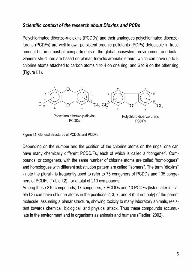
Polychlorinated dibenzo-p-dioxins (PCDDs) and their analogues polychlorinated dibenzo-
furans (PCDFs) are well known persistent organic pollutants (POPs) detectable in trace
amount but in almost all compartments of the global ecosystem, environment and biota.
General structures are based on planar, tricyclic aromatic ethers, which can have up to 8
chlorine atoms attached to carbon atoms 1 to 4 on one ring, and 6 to 9 on the other ring
(Figure I.1).
Figure I.1: General structures of PCDDs and PCDFs.
Depending on the number and the position of the chlorine atoms on the rings, one can
have many chemically different PCDD/Fs, each of which is called a “congener”. Com-
pounds, or congeners, with the same number of chlorine atoms are called “homologues”
and homologues with different substitution pattern are called “isomers”. The term “dioxins”
- note the plural - is frequently used to refer to 75 congeners of PCDDs and 135 conge-
ners of PCDFs (Table I.2), for a total of 210 compounds.
Among these 210 compounds, 17 congeners, 7 PCDDs and 10 PCDFs (listed later in Ta-
ble I.3) can have chlorine atoms in the positions 2, 3, 7, and 8 (but not only) of the parent
molecule, assuming a planar structure, showing toxicity to many laboratory animals, resis-
tant towards chemical, biological, and physical attack. Thus these compounds accumu-
late in the environment and in organisms as animals and humans (Fiedler, 2002).
Polychloro dibenzo-p-dioxins
PCDDs Polychloro dibenzofurans
PCDFs
6
Table I.2: Possible number of isomers within homologue groups for PCDD and PCDF.
Homologue PCDD isomers PCDF isomers
Monochloro- 2 4
Dichloro- 10 16
Trichloro- 14 28
Tetrachloro- 22 38
Pentachloro- 14 28
Hexachloro- 10 16
Heptachloro- 2 4
Octachloro- 1 1
Total 75 135
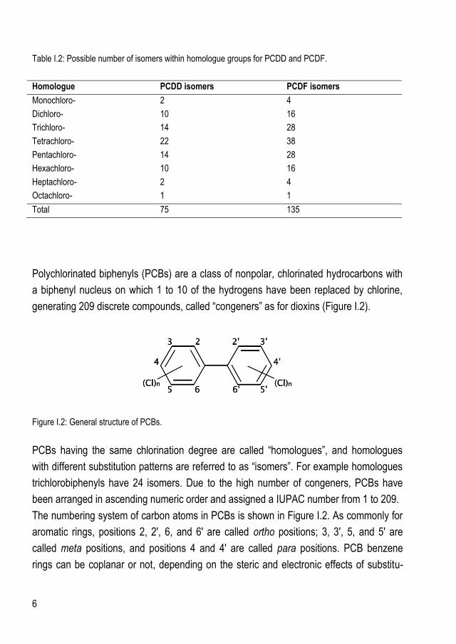
Polychlorinated biphenyls (PCBs) are a class of nonpolar, chlorinated hydrocarbons with
a biphenyl nucleus on which 1 to 10 of the hydrogens have been replaced by chlorine,
generating 209 discrete compounds, called “congeners” as for dioxins (Figure I.2).
Figure I.2: General structure of PCBs.
PCBs having the same chlorination degree are called “homologues”, and homologues
with different substitution patterns are referred to as “isomers”. For example homologues
trichlorobiphenyls have 24 isomers. Due to the high number of congeners, PCBs have
been arranged in ascending numeric order and assigned a IUPAC number from 1 to 209.
The numbering system of carbon atoms in PCBs is shown in Figure I.2. As commonly for
aromatic rings, positions 2, 2', 6, and 6' are called ortho positions; 3, 3', 5, and 5' are
called meta positions, and positions 4 and 4' are called para positions. PCB benzene
rings can be coplanar or not, depending on the steric and electronic effects of substitu-

7
ents, especially in the otho position, where the replacement of hydrogen atoms with larger
chlorine atoms forces the benzene rings to rotate out of the planar configuration.
The benzene rings of non-ortho substituted PCBs assume a planar configuration and so
these compounds can be called “coplanar congeners” (co-PCBs). Also some mono-ortho
(MO-) substituted PCB congeners are planar. The benzene rings of those PCBs having
more than two chlorine atoms in ortho position cannot assume a planar configuration and
are indicated as “non-planar congeners”. The chlorination pattern of the PCBs determines
the final PCB spatial configuration and also the toxicity of the substance as explained in
the following paragraph.
1. Dioxin and PCB structure related toxicity
Among dioxins, 2,3,7,8-tetrachloro dibenzo-p-dioxin (2,3,7,8-TCDD) is considered the
most toxic compound, as it has one of the lowest known LD50 (lethal dose to 50% of the
population) values. It takes only 0.6 μg/kg of body weight to kill male guinea pigs
(Schwetz B.A., 1973, Fiedler, 2002). The polychlorinated dibenzofurans are only slightly
less toxic; for example, the LD50 of 2,3,7,8-TCDF is about 6 μg/kg for male guinea pigs
(Van den Berg et al., 2006). It is important to underline that the toxicity of dioxins varies
dramatically from species to species; for example, 2,3,7,8-TCDD is about 500 times less
toxic to rabbits than it is to guinea pigs. Other 2,3,7,8-substituted dioxin and furan conge-
ners are also toxic, and many of these compounds have both acute and chronic effects.
PCDD and PCDF toxicity is related mainly to their capacity to interact with the cytosolic
specific protein called the aryl hydrocarbon receptor (AhR). The binding to the Ah recep-
tor constitutes a first and necessary step to initiate the toxic and biochemical effects. Di-
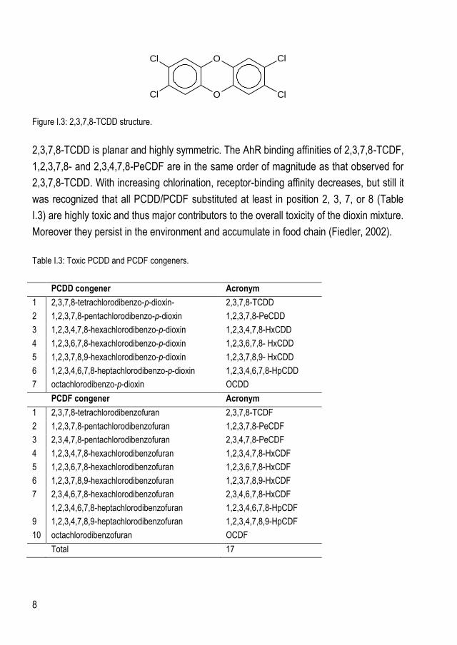
oxin 2,3,7,8-TCDD (Figure I.3) is the congener with the highest affinity to AhR and so it is
the most toxic PCDD congener.
8
O
O
Cl
Cl
Cl
Cl
Figure I.3: 2,3,7,8-TCDD structure.
2,3,7,8-TCDD is planar and highly symmetric. The AhR binding affinities of 2,3,7,8-TCDF,
1,2,3,7,8- and 2,3,4,7,8-PeCDF are in the same order of magnitude as that observed for
2,3,7,8-TCDD. With increasing chlorination, receptor-binding affinity decreases, but still it
was recognized that all PCDD/PCDF substituted at least in position 2, 3, 7, or 8 (Table
I.3) are highly toxic and thus major contributors to the overall toxicity of the dioxin mixture.
Moreover they persist in the environment and accumulate in food chain (Fiedler, 2002).
Table I.3: Toxic PCDD and PCDF congeners.
PCDD congener Acronym
1 2,3,7,8-tetrachlorodibenzo-p-dioxin- 2,3,7,8-TCDD
2 1,2,3,7,8-pentachlorodibenzo-p-dioxin 1,2,3,7,8-PeCDD
3 1,2,3,4,7,8-hexachlorodibenzo-p-dioxin 1,2,3,4,7,8-HxCDD
4 1,2,3,6,7,8-hexachlorodibenzo-p-dioxin 1,2,3,6,7,8- HxCDD
5 1,2,3,7,8,9-hexachlorodibenzo-p-dioxin 1,2,3,7,8,9- HxCDD
6 1,2,3,4,6,7,8-heptachlorodibenzo-p-dioxin 1,2,3,4,6,7,8-HpCDD
7 octachlorodibenzo-p-dioxin OCDD
PCDF congener Acronym
1 2,3,7,8-tetrachlorodibenzofuran 2,3,7,8-TCDF
2 1,2,3,7,8-pentachlorodibenzofuran 1,2,3,7,8-PeCDF
3 2,3,4,7,8-pentachlorodibenzofuran 2,3,4,7,8-PeCDF
4 1,2,3,4,7,8-hexachlorodibenzofuran 1,2,3,4,7,8-HxCDF
5 1,2,3,6,7,8-hexachlorodibenzofuran 1,2,3,6,7,8-HxCDF
6 1,2,3,7,8,9-hexachlorodibenzofuran 1,2,3,7,8,9-HxCDF
7 2,3,4,6,7,8-hexachlorodibenzofuran 2,3,4,6,7,8-HxCDF
1,2,3,4,6,7,8-heptachlorodibenzofuran 1,2,3,4,6,7,8-HpCDF
9 1,2,3,4,7,8,9-heptachlorodibenzofuran 1,2,3,4,7,8,9-HpCDF
10 octachlorodibenzofuran OCDF
Total 17

9
In this manuscript, the terms “dioxin“ and “dioxins” should be interpreted as including
these selected polychlorinated dibenzo-p-dioxins and polychlorinated dibenzofurans
showing high toxicity and for this reason regulated from the EU.
Based on structural characteristics and toxicological effects, PCBs are divided into dioxin-
like PCBs (DL-PCBs) showing toxicological properties similar to dioxins and non dioxin-
like PCBs (NDL-PCBs) which do not share the dioxin’s toxic mechanism of AhR binding
(European Food Safety Authority, 2010), but their toxicological effects are related to dif-
ferent action mechanisms. PCB congeners showing dioxin-like toxicity have planar and
symmetric spatial configuration due to their chlorination pattern, and in fact they are non-
ortho-PCBs, 4 congeners indicated also as coplanar PCBs (co-PCBs), and 8 mono-ortho
(MO-) PCBs with only one chlorine atom in ortho position. It is the planar structure that
leads to the same toxicity as the dioxins, and in fact the most toxic PCB congeners,
namely, 3,3',4,4',5-pentachlorobiphenyl (PCB 126) and 3,3',4,4',5,5'-hexachlorobiphenyl
(PCB 169) are approximate isostereomers of 2,3,7,8-TCDD, whit similar structural and
spatial configuration (Safe S. et al., 1985). Toxic DL-PCBs and are listed in Table I.4.
Cl
Cl Cl
Cl
Cl
Cl
Cl Cl
Cl
Cl
Cl
PCB 126 PCB 169
Figure I.4: Examples of planar structure of the two most toxic dioxin-like PCBs.
10
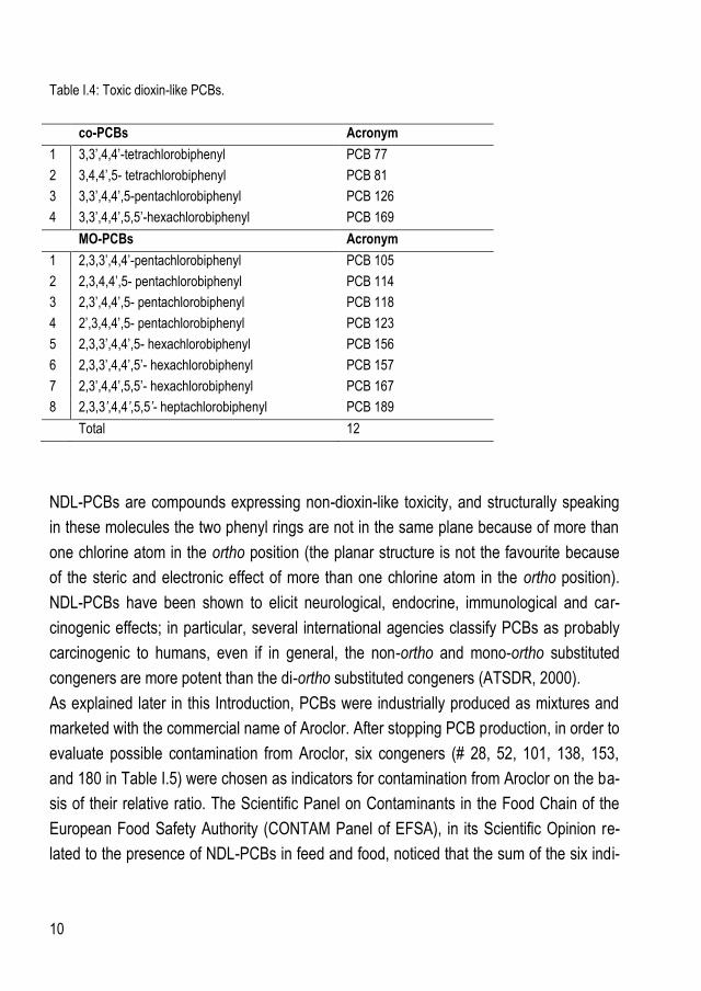
Table I.4: Toxic dioxin-like PCBs.
co-PCBs Acronym
1 3,3’,4,4’-tetrachlorobiphenyl PCB 77
2 3,4,4’,5- tetrachlorobiphenyl PCB 81
3 3,3’,4,4’,5-pentachlorobiphenyl PCB 126
4 3,3’,4,4’,5,5’-hexachlorobiphenyl PCB 169
MO-PCBs Acronym
1 2,3,3’,4,4’-pentachlorobiphenyl PCB 105
2 2,3,4,4’,5- pentachlorobiphenyl PCB 114
3 2,3’,4,4’,5- pentachlorobiphenyl PCB 118
4 2’,3,4,4’,5- pentachlorobiphenyl PCB 123
5 2,3,3’,4,4’,5- hexachlorobiphenyl PCB 156
6 2,3,3’,4,4’,5’- hexachlorobiphenyl PCB 157
7 2,3’,4,4’,5,5’- hexachlorobiphenyl PCB 167
8 2,3,3’,4,4’,5,5’- heptachlorobiphenyl PCB 189
Total 12
NDL-PCBs are compounds expressing non-dioxin-like toxicity, and structurally speaking
in these molecules the two phenyl rings are not in the same plane because of more than
one chlorine atom in the ortho position (the planar structure is not the favourite because
of the steric and electronic effect of more than one chlorine atom in the ortho position).
NDL-PCBs have been shown to elicit neurological, endocrine, immunological and car-
cinogenic effects; in particular, several international agencies classify PCBs as probably
carcinogenic to humans, even if in general, the non-ortho and mono-ortho substituted
congeners are more potent than the di-ortho substituted congeners (ATSDR, 2000).
As explained later in this Introduction, PCBs were industrially produced as mixtures and
marketed with the commercial name of Aroclor. After stopping PCB production, in order to
evaluate possible contamination from Aroclor, six congeners (# 28, 52, 101, 138, 153,
and 180 in Table I.5) were chosen as indicators for contamination from Aroclor on the ba-
sis of their relative ratio. The Scientific Panel on Contaminants in the Food Chain of the
European Food Safety Authority (CONTAM Panel of EFSA), in its Scientific Opinion re-
lated to the presence of NDL-PCBs in feed and food, noticed that the sum of the six indi-

11
cator PCBs represented about 50% of the total NDL-PCB in food (European Food Safety
Authority, 2010). For this reason NDL-PCBs are also referred to as “indicator PCBs” (I-
PCBs).
Table I.5: List of I-PCBs.
I-PCBs Acronym
1 2,4,4’-trichorobiphenyl PCB 28
2 2,2’,5,5’-tetrachorobiphenyl PCB 52
3 2,2’,4,5,5’-pentachorobiphenyl PCB 101
4 2,2’,3,4,4’,5’-hexachorobiphenyl PCB 138
5 2,2’,4,4’,5,5’- hexachorobiphenyl PCB 153
6 2,2',3,4,4',5,5'-heptachlorobiphenyl PCB 180
Total 6
2. Dioxin sources and environmental contamination
PCDDs and PCDFs were never produced intentionally as marketable products but they
were unwanted by-products of industrial and combustion processes (Hites, 2011), that
are considered “primary sources” (Fiedler, 2002). Due to their chemical, physical and bio-
logical stability PCDD/PCDF from “primary sources” are transferred to other matrices and
enter the environment. Such “secondary sources” are sewage sludge/biosludge, compost,
or contaminated soils and sediments.
2.1. Primary sources
Primary sources of environmental contamination with PCDD/PCDF in the past were due
to production and use of chloro-organic chemicals. The propensity to generate
PCDD/PCDF during synthesis of chemical compounds decreases in the following order:
chlorophenols>chlorobenzenes>aliphatic chlorinated compounds>inorganic chlorinated
compounds. Factors favourable for the formation of PCDD/PCDF are high temperatures,
alkaline media, presence of UV-light, and presence of radicals in the reaction mix-
ture/chemical process (Fiedler, 2002).

12
One of the classic example is the formation of 2,3,7,8-TCDD as by-product in the produc-
tion of 2,4,5-trichlorophenol (also known as Dowicide 2, one product in the Dowicide an-
timicrobial series from Dow chemical company), which was synthesized by the reaction of
1,2,4,5-tetrachlorobenzene with sodium hydroxide (NaOH). Dimerization of the resulting
2,4,5-trichlorophenol produced small amounts of 2,3,7,8-TCDD, which contaminated the
final commercial product (Figure I.5)
Cl Cl
Cl Cl
NaOH
Cl OH
Cl Cl
Cl OH
Cl Cl ClOH
ClCl- 2 HCl
O
O
Cl
Cl
Cl
Cl
2,4,5-trichlorophenol 2,3,7,8-tetrachlorodibenzo-p-dioxin
+
Figure I.5: 2,4,5-trichlorophenol dimerization in acidic media forming 2,3,7,8-tetrachlorodibenzo-p-dioxin.
Although dioxins were present at very low levels in some commercial products, they en-
tered the environment with uncontrolled release, causing very big environmental and
health issues for animals and human, as described in some examples in the following
paragraph about secondary sources of contamination.
At the present, changes in industrial processes have resulted in the reduction of
PCDD/PCDF contamination in other products, but still a little amount of PCDD/PCDF into
the environment via water and to soils derives also from kraft pulp (process for the pro-
duction of pure cellulose fibres from lignin in alkali conditions) and paper mills, because of
the wood treated with pentachlorophenol (PCP) or other chlorinated preservatives. Other
PCP treated materials include textiles, leather goods, and cork products. However, to-
day’s dioxin input is mainly due to thermal processes. One (but not the only) of several
examples) are waste incinerators, that are burning together a great variety of entry mate-
rials, at high temperature, in excess of oxygen and in presence of a catalyst. In these

13
conditions carbon and chlorine containing materials (PVC, chloroparaffines, organic dyes
or inorganic chlorine are just little examples) lead easily to dioxin production. Most recent
technology is aimed to reduce emissions of PCDD/Fs in the environment but it does occur
in some extent.
PCB based electric fluids are another important source of contamination from dioxins in
landfills.
2.2. Secondary sources
Secondary sources of PCDD/PCDFs are environmental and biota matrices contaminated
by the primary emission sources and after the accidental contamination happened in the
past, where toxicological effects of dioxins were not yet known.
Likely the first example of dioxin accidents was the “Chick Edema Disease” occurred in
1957 in the US, when millions of checks died mysteriously (Hites, 2011). After several re-
searches, cause was traced to the fatty acids added to the chicken’s feed and coming
from hides for tanning industry. Fatty acids in fact were produced from the saponification
of the fat removed from animal hides. In the end of the ‘50s, 2,3,4,6-tetrachlorophenol
(sold as Dowicide 6) was added as a preservative to hides for tanning industry. Removed
fat saponification caused tetrachlorophenol dimerization and 1,2,3,7,8,9- and 1,2,3,6,7,8-
hexachlorodibenzo-p-dioxin production (similar reaction as reported in Figure I.5), that
contaminated fatty acids for feed.
Another historical example happened in Vietnam where in the ‘70s, 2,4,5-trichlorophenol
and hence 2,3,7,8-TCDD (see Figure I.5) were contaminants of the herbicide Agent Or-
ange used by the U.S in large amount during the war in Vietnam (from 1955 to 1975).
This caused proven environmental and health problems to veterans exposed to Agent
Orange, whose tumour incidence was higher than the average.
In the ‘60s in a city called Times Beach in Missouri, chemical waste oil containing kilo-
grams of 2,3,7,8-TCDD was first withdrawn for disposal, but then mixed with other waste
oils and re-used for several purposes, as for example spray for indoor dust control. This
“ingenuousness” caused animal death and environmental issues.

14
A very famous accident occurred in Europe, in Italy, in a northern town called Seveso,
where in 1976 chemicals from a production plant using 2,4,5-trichlorophenol, and hence
producing dioxins as by-products, were released into the environment as a safety meas-
ure for vessel overpressure. Within few days in that area chicken and rabbits died and
children had first skin diseases. The area was immediately evacuated for decontamina-
tion, with social and economic consequences. With the time, several chloracne cases
were recorded among exposed people, as well as higher female children natality from ex-
posed fathers.
Unfortunately the list of accident of dioxin contamination is longer and some other exam-
ples are reported later because they involve also PCBs.
2.3. Fate and transport
Due to their high lipophilicity and low water solubility, after their introduction in the envi-
ronment, PCDD/PCDFs are primarily bound to particulate and organic matter in soil and
sediments. Their resistance to degradation and semi-volatility caused their transport over
long distances and their past released into the environment still contributes to contempo-
rary exposure. Despite their low solubility, dioxins are slowly released from sediments into
water and they can be adsorbed by biota, assimilated by small fishes and so enter the
food chain. Due to their lipophilicity and metabolic resistance, they are concentrated and
accumulated in fatty tissues and tend to bioaccumulate in higher animals, including hu-
mans (Buckley-Golder, 1999).

15
3. PCB sources and fate
3.1. Industrial production
Contrary to PCDDs and PCDFs, PCBs were industrially produced as complex mixtures of
several congeners for a variety of uses, including dielectric fluids, capacitor and trans-
former components because of their good electrical insulating properties, as well as addi-
tives in plasticizers or lubricants. PCBs were used in minor extent also in pesticides, inks,
paints, flame retardants and many other applications. (Erickson, 1997). The list of PCB
uses is very long and it involves common domestic goods; their chemical and physical
stability led to their commercial utility on one side and to environmental contamination
problem on the other side.
PCBs were produced via direct chlorination of biphenyl with gaseous chlorine at high
temperature and in presence of FeCl2 as catalyst. The extent of chlorination was con-
trolled with reaction time (Figure I.6).
+ Cl Cl (gas)
Clx Cly
Biphenyl Polychlorobiphenyls
FeCl2
Figure I.6: PCB general production reaction.
The major producer was the USA with Monsanto Corporation (St. Louis, MO) that mar-
keted PCBs under the name Aroclor®. But, due to their commercial importance, PCBs
were produced all over the world as shown in Table I.6 (Breivik et al., 2002)
16
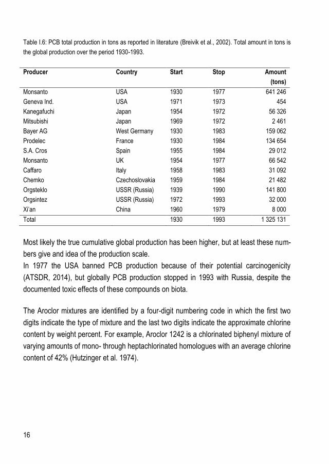
Table I.6: PCB total production in tons as reported in literature (Breivik et al., 2002). Total amount in tons is
the global production over the period 1930-1993.
Producer Country Start Stop Amount
(tons)
Monsanto USA 1930 1977 641 246
Geneva Ind. USA 1971 1973 454
Kanegafuchi Japan 1954 1972 56 326
Mitsubishi Japan 1969 1972 2 461
Bayer AG West Germany 1930 1983 159 062
Prodelec France 1930 1984 134 654
S.A. Cros Spain 1955 1984 29 012
Monsanto UK 1954 1977 66 542
Caffaro Italy 1958 1983 31 092
Chemko Czechoslovakia 1959 1984 21 482
Orgsteklo USSR (Russia) 1939 1990 141 800
Orgsintez USSR (Russia) 1972 1993 32 000
Xi’an China 1960 1979 8 000
Total 1930 1993 1 325 131
Most likely the true cumulative global production has been higher, but at least these num-
bers give and idea of the production scale.
In 1977 the USA banned PCB production because of their potential carcinogenicity
(ATSDR, 2014), but globally PCB production stopped in 1993 with Russia, despite the
documented toxic effects of these compounds on biota.
The Aroclor mixtures are identified by a four-digit numbering code in which the first two
digits indicate the type of mixture and the last two digits indicate the approximate chlorine
content by weight percent. For example, Aroclor 1242 is a chlorinated biphenyl mixture of
varying amounts of mono- through heptachlorinated homologues with an average chlorine
content of 42% (Hutzinger et al. 1974).

17
Table I.7: Average molecular composition (wt%) of some Aroclor.
Homologues Aroclor
1221 1232 1016 1242 1248 1254 1260
0 10
1 50 26 2 1
2 35 29 19 13 1
3 4 24 57 45 22 1
4 1 15 22 31 49 15
5 10 27 53 12
6 2 26 42
7 4 38
8 7
9 1
As reported in Table I.7 main constituents of commercial mixtures are homologues with 3
to 7 chlorine atoms, which include very toxic DL-PCBs and NDL-PCBs, that therefore are
used as indicators of contamination from Aroclor mixtures.
Among other impurities, commercial PCB mixtures contained tetra- and penta-CDF con-
geners as reaction by-products. The presence of PCDFs in PCB mixtures has been
documented at µg/g level (part per million, ppm) and may account for some toxicological
properties of PCB mixtures; PCDDs have not been found in marketed products (Erickson,
1997).
3.2. Secondary sources
Secondary PCB sources, after the stop of their production, are industrial processes where
PCBs are produced as by-products, and items already containing PCBs, that release
them with time. Outdated or illegal landfills are new sources of PCBs, as well as the burn-
ing of PCB-containing products, that has introduced large volumes of PCBs into the envi-
ronment.
PCBs can incidentally be produced as by-products of other industrial processes using hy-
drocarbons and chlorine. These by-products are referred to as “incidental PCBs”. Indus-
trial processes include manufacture of chlorinated solvents, chlorinated alkanes or some
18
pigments, as well as the thermal degradation of waste in incinerators. In all these cases,
the composition and the amount of by-products is not exactly known and traceable
(Erickson, 1997).
Due to the long service life of many PCB-containing items and the use of PCBs in some
durable, relatively inert products, PCB-containing materials are still currently disposed
and processed in waste and recycling operations, that can be a new source of PCBs if
operations are not carried out properly (EPA, 2003).
PCBs are present in building demolition material, not always properly disposed of; they
are in dumps, landfills and wastewater treatment plant sludge, and sometimes they enter
the environment because of the releases into sewers and streams, improper disposal of
PCB-containing equipment in non-secured landfill sites and municipal disposal facilities,
and by other routes (such as sea dumping).
In the past, PCB food contamination episodes have occurred and they introduced big
quantities of toxic persistent compounds (PCBs and their contaminants) in the food chain.
Just an example was the “Yusho” accident, in Japan in 1968 (Tanabe et al., 1987) and
the analogue “Yu-Cheng” accident in Taiwan in 1979 (Soongl D. K., 1997) where rice oil
for food was accidentally mixed with PCB containing oil used as heat exchange fluid in
the production factory.
In Europe, namely in France in the ‘ 70s, French cheese was accidentally contaminated
with technical oil from farm engines and some poultry was poisoned with PCB-
contaminated plastic wire netting; accident happened also in The Netherlands and in
Germany in the ‘80s and ‘90s, contaminating environment, food and feed with dioxins and
PCBs (Covaci et al., 2008). But it was in 1999 that the most mediatised crisis occurred
and it was the “Belgian PCB/dioxin crisis”, when PCB containing transformer waste oil
was inadvertently mixed with recycled fats used in the production of animal feeds and fur-
ther distributed to chicken and pig farms. PCB oil was contaminated with dioxins and this
resulted in the slaughter of thousands of animals, with resulting political and economic
crisis.

19
3.3. Fate and transport
Some of the PCB commercial mixtures applications were “open ended” (component of
dust control formulations, paints, and inks, carbonless copy paper, flame retardants, pes-
ticide additives) and resulted in widespread low level releases to environmental compart-
ments. Closed and controlled uses, such as dielectrics within electric equipment have still
resulted in environmental release because of spills, improper handling and improper dis-
posal. This caused local but very high concentration contamination. Once in the environ-
ment, PCBs had the same fate as dioxins because of similar chemical and physical prop-
erties, such as high lipophilicity and stability. PCBs were adsorbed on the organic matter
of sediments and soil. With time they have been transported also to remote areas and
widespread in different sites, so that, at the present, PCBs are ubiquitous environmental
pollutants.
PCBs volatilize from both soil and water, and once in gas phase, they can be transported
long distances in air, and then redeposited by settling or scavenging by precipitation. This
cycling process continues indefinitely and is referred to as the grasshopper effect (EPA,
2001). Clear evidence of the atmospheric deposition of PCBs is the presence of PCBs in
remote areas of the planet and their accumulation in polar bears. From the environment,
they were taken up by small organisms and fishes and entered the food chain, where they
tend to bio-accumulate as dioxins: PCBs have been found in animal adipose samples,
milk, sediments and numerous other matrices.
4. Risk assessment, Toxic Equivalent Factor (TEF) and European Regulation
Media and public opinion spotlighted the Belgian dioxin crisis and the lack of food safety,
so early in 2000 the European Union (EU) was pushed to start an efficient monitoring
program to ensure the proper quality of European food and feed (Focant, 2012). As a
consequence, starting from 2000, the European Commission (EC) began to propose leg-
islation to regulate Maximum Residual Levels (MLs) for PCDDs, PCDFs and DL-PCBs in
foodstuffs and feed products, as well as guidelines for analytical methods to support and
implement continuous monitoring of food and feed. PCDDs, PCDFs and PCBs exist as

20
mixtures of congeners and this complicates the risk evaluation. As all these chemicals
have similar actions on the AhR but different potencies, a toxic equivalent factor (TEF)
was developed to assess the impact of all these compounds on human and environ-
mental health, as well as for regulatory control of exposure to these mixtures.
TEF values are based on the relative toxicity of a chemical in comparison with 2,3,7,8-
TCDD, which is the most toxic congener with a TEF value of 1. Other 2,3,7,8-substituted
PCDD, PCDF and PCB congeners, with similar planar structure, and hence similar inter-
actions with AhR receptor, have been assigned a TEF value. In 1997 an expert meeting
was organized in Stockholm by the World Health Organization (WHO) to determine TEF
values for specific congeners based on existing literature toxicological data available at
that moment (Van.den.Berg et al., 1998). Included congeners had
Structural similarity to 2,3,7,8-TCDD
Capacity to bind to the aryl hydrocarbon receptor (AhR);
Capacity to elicit AhR-mediated biochemical and toxic responses;
Persistence and accumulation in the food chain
In 2005, a further WHO expert panel updated TEF values for dioxin-like compounds (Van
den Berg et al., 2006). They reaffirmed the characteristics necessary for the inclusion of a
compound in the WHO‘s TEF list, but they changed TEF value for some congener based
on new and updated toxicological data. As said, 2,3,7,8-TCDD is the most toxic congener
with a TEF value of 1 and all other congeners have lower TEFs ranging from 0.00001 to
0.5 (Table I.8).
Table I.8: WHO 1198 and 2005 TEF values for dioxin-like compounds. Numbers in bold indicate a change
in TEF values from 1998 to 2005
Compound WHO 1998 TEF WHO 2005 TEF
PCDDs
1 2,3,7,8-TCDD 1 1
2 1,2,3,7,8-PeCDD 1 1
3 1,2,3,4,7,8-HxCDD 0.1 0.1
4 1,2,3,6,7,8-HxCDD 0.1 0.1

21
5 1,2,3,7,8,9-HxCDD 0.1 0.1
6 1,2,3,4,6,7,8-HpCDD 0.01 0.01
7 OCDD 0.001 0.0003
PCDFs
1 2,3,7,8-TCDF 0.1 0.1
2 1,2,3,7,8-PeCDF 0.05 0.03
3 2,3,4,7,8-PeCDF 0.5 0.3
4 1,2,3,4,7,8-HxCDF 0.1 0.1
5 1,2,3,6,7,8-HxCDF 0.1 0.1
6 1,2,3,7,8,9-HxCDF 0.1 0.1
7 2,3,4,6,7,8-HxCDF 0.1 0.1
8 1,2,3,4,6,7,8-HpCDF 0.01 0.01
9 1,2,3,4,7,8,9-HpCDF 0.01 0.01
10 OCDF 0.0001 0.0003
co-PCBs
1 PCB 77 0.0001 0.0001
2 PCB 81 0.0001 0.0003
3 PCB 126 0.1 0.1
4 PCB 169 0.01 0.03
MO-PCBs
1 PCB 105 0.0001 0.00003
2 PCB 114 0.0005 0.00003 3 PCB 118 0.0001 0.00003 4 PCB 123 0.0001 0.00003 5 PCB 156 0.0005 0.00003 6 PCB 157 0.0005 0.00003 7 PCB 167 0.00001 0.00003 8 PCB 180 0.0001 0.00003
Risk assessment based on the TEF approach starts from the important assumption that
the combined effects of the different congeners are dose or concentration additive. There-
fore, TEF values of each congener, multiplied by its concentration, can be used to calcu-
late the toxic equivalent (TEQ) concentration of an environmental or biological sample.
TEQ calculation is based on the following formula, and allows the estimation of sample
global toxicity.

22
TEFs and TEQs are used for risk characterization and regulation purposes because they
allow converting quantitative analytical data for individual PCDD/PCDF and PCB conge-
ners into a single parameter representing the global toxicity of the sample, the TEQ. At
the present the reference regulation for maximum residual levels (MLs) of dioxins in food
and feed stuff in Europe are based on TEQ levels and the most recent are the EU Regu-
lation 1881/2006 with all its amendments for food, and the Directive 2002/32/CE with all
its amendments for MLs in feed.
In order to support a continuous monitoring program for food and feed safety in Europe
and ensure rapid action in case of non-compliant samples, dedicate legislation was done
by the EC for analytical methods of sampling and analysis for the control of PCDD/Fs and
DL-PCBs in food and feed. The most recent versions are the Commission Regulation
589/2014 for analytical methods for quantitative analysis in food, and the Commission
Regulation 709/2014 for analytical methods for quantitative analysis in feed, both re-
leased as amendments of previous Regulation arisen after the Belgian dioxin crisis.
These Regulations describe the criteria to meet when doing dioxin analysis for confirma-
tory or screening purposes without laying down just one analytical method to follow, so
actually there is a great variety of an analytical procedures to perform dioxin and PCB
analysis in food and feed, from sample preparation to instrumental detection. In particular
a major recent update is the recognition of gas chromatography (GC) triple quadrupole
mass spectrometry (GC-MS/MS Triple Quad) as a confirmatory tool for checking compli-
ance with MLs. Triple Quad instruments are cheaper and more widespread instruments
than Magnetic Sector high resolution mass spectrometers (HRMS), and so, thanks to this
modification in the EU Regulation, the number of laboratories participating to food safety
monitoring program can increase.
In this thesis dioxin analysis has been carried out on the basis of the routine procedure
developed in our laboratory (CART at the University of Liège). This procedure has been

23
modified in the sample preparation part related to the automated clean-up, with the aim of
reducing solvent and time consumption, in order to have more environmental sustainable,
cheaper and faster procedures. From the instrumental point of view, a validated method
based on GC-MS/MS Triple Quad instrument (L'Homme et al., 2015b) has been used to
assess the recoveries of the alternative clean-up methods, as described in Chapters 1, 2
and 3. Chapter 1 reports the description of the instrumental method and all the steps fol-
lowed for its validation. The work load of the author of this thesis has been related to
method optimization and continue usage, rather than to the initial development.

24
Scientific context of the research about Dechloranes
Dechloranes are organo-chlorinated compounds sharing a bicycle [2,2,1] heptane struc-
ture. The first of these compounds was called Mirex, or Dechlorane, and it was exten-
sively used as pesticide and as additive for flame retardants in the USA during the ‘60s
and the ‘70s until 1978 when it was banned because of its toxicity, persistence and bioac-
cumulation (Kaiser, 1978). In fact Mirex is in the POPs list of the Stockholm convention
(Table I.1), but other Dechloranes, namely Dechlorane Plus, syn- and anti-isomers, (DP),
Dechlorane 602 (Dec 602), Dechlorane 603 (Dec 603,), Dechlorane 604 (Dec 604),
Chlordene Plus (CP) are unregulated and they are currently used as replacement of
Mirex or decabromodiphenyl ether (deca-BDE, BDE-209) for their pesticide and flame re-
tardant properties. They are extensively used as additives in various synthetic products
such as nylon or plastic like polypropylene, as well as in electronic devices (Sverko et al.,
2011). They have recently been reported at low levels in environmental samples, or in
dust collected from various environments (Dodson et al., 2012, Cao et al., 2014). Biota
and humans are exposed to these chemicals and in fact very recent human biomonitoring
studies have reported levels at the ng/g lipid level in breast milk from Canada (Zhou et al.,
2014), as well as in human serum from Norway (Cequier et al., 2015) and France
(Brasseur et al., 2014), even though no production sources have been found in Europe.
In this thesis, with the goal of understanding the extent and the origin of human exposure
to Dechloranes, food consumption was investigated as a possible route of exposure for
people from Belgium, as, due to their similarity to Mirex, other Dechloranes can be sub-
ject to bioaccumulation and long range transport. Because of the emerging character of
these analytes, the first part of the study has been dedicated to the development of a
specific method for the analysis of 6 Dechloranes (Dec 604 was not detectable at the
level of interest). The sample preparation procedure currently applied for dioxin analysis
demonstrated to be suitable for Dechlorane analysis; final extracts were injected and
quantitated by means of GC-MS/MS Triple Quad, while usually HRMS instruments have
been used for such compounds; the method was validated following the applicable guide-
lines of the stringent EU Regulation for dioxin analysis (589/2014 and 709/2014), and fi-
nally Dechlorane levels have been assessed in 88 selected food and feed samples to
produce a first estimate of Dechlorane dietary intake for the Belgian population. Details

25
are reported in Chapter 4. The results of this work have been published in peer-reviewed
journal.
26
Bibliography
ATSDR, 2014. ATSDR Case Studies in Environmental Medicine Polychlorinated Biphenyls (PCBs) Toxicity. AGENCY FOR TOXIC SUBSTANCES AND DISEASE REGISTRY.
ATSDR, U. S. D. O. H. A. H. S. P. H. S.-A. F. T. S. A. D. R. 2000. TOXICOLOGICAL PROFILE FOR POLYCHLORINATED BIPHENYLS (PCBs).
BRASSEUR, C., PIRARD, C., SCHOLL, G., DE PAUW, E., VIEL, J. F., SHEN, L., REINER, E. J. & FOCANT, J. F. 2014. Levels of dechloranes and polybrominated diphenyl ethers (PBDEs) in human serum from France. Environment International, 65, 33-40.
BREIVIK, K., SWEETMAN, A., PACYNA, J. M. & JONES, K. C. 2002. Towards a global historical emission inventory for selected PCB congeners - A mass balance approach: 1. Global production and consumption. Science of the Total Environment, 290, 181-198.
BUCKLEY-GOLDER, D. 1999. Compilation of EU Dioxin Exposure and Health Data - Summary Report.
CAO, Z., XU, F., COVACI, A., WU, M., WANG, H., YU, G., WANG, B., DENG, S., HUANG, J. & WANG, X. 2014. Distribution patterns of brominated, chlorinated, and phosphorus flame retardants with particle size in indoor and outdoor dust and implications for human exposure. Environmental Science and Technology, 48, 8839-8846.
CEQUIER, E., SAKHI, A. K., MARCÉ, R. M., BECHER, G. & THOMSEN, C. 2015. Human exposure pathways to organophosphate triesters - A biomonitoring study of mother-child pairs. Environment International, 75, 159-165.
COVACI, A., VOORSPOELS, S., SCHEPENS, P., JORENS, P., BLUST, R. & NEELS, H. 2008. The Belgian PCB/dioxin crisis-8 years later. An overview. Environmental Toxicology and Pharmacology, 25, 164-170.
DI LEO, A., ANNICCHIARICO, C., CARDELLICCHIO, N., GIANDOMENICO, S., CONVERSANO, M., CASTELLANO, G., BASILE, F., MARTINELLI, W., SCORTICHINI, G. & SPADA, L. 2014. Monitoring of PCDD/Fs and dioxin-like PCBs and seasonal variations in mussels from the Mar Grande and the Mar Piccolo of Taranto (Ionian Sea, Southern Italy). Environmental Science and Pollution Research, 21, 13196-13207.
DODSON, R. E., PEROVICH, L. J., COVACI, A., VAN DEN EEDE, N., IONAS, A. C., DIRTU, A. C., BRODY, J. G. & RUDEL, R. A. 2012. After the PBDE phase-out: A broad suite of flame retardants in repeat house dust samples from California. Environmental Science and Technology, 46, 13056-13066.
EPA 2001. Frequently Asked Questions About Atmospheric Deposition. EPA 2003. EPA Fact Sheet: Sources of Polychlorinated Biphenyls. PCB fact sheet.cp.8-6-03.doc. ERICKSON, M. D. 1997. Analytical Chemistry of PCBs - Second Edition, Lewis Publisher. EUROPEAN FOOD SAFETY AUTHORITY, E. 2010. Results of the monitoring of non dioxin-like
PCBs in food and feed. SCIENTIFIC REPORT OF EFSA. EFSA. FIEDLER, H. 2002. Persistent Organic Pollutants. FOCANT, J. F. 2012. Dioxin food crises and new POPs: Challenges in analysis. Analytical and
Bioanalytical Chemistry, 403, 2797-2800. HITES, R. A. 2011. Dioxins: An overview and history. Environmental Science and Technology, 45,
16-20.

27
KAISER, K. L. E. 1978. Pesticide Report: The rise and fall of mirex. Environmental Science & Technology, 12, 520-528.
L'HOMME, B., SCHOLL, G., EPPE, G. & FOCANT, J. F. 2015. Validation of a gas chromatography-triple quadrupole mass spectrometry method for confirmatory analysis of dioxins and dioxin-like polychlorobiphenyls in feed following new EU Regulation 709/2014. Journal of Chromatography A, 1376, 149-158.
SAFE S., B. S., SAWYER T., ROBERTSON L., S. L., PARKINSON A., THOMAS P.E. & , R. D. E., REIK L.M., LEVIN W., DENOMMET M.A. AND FUJITA T. 1985. PCBs: Structure-Function Relationships and Mechanism of Action. Environmental Health Perspectives, 60, 47-56.
SCHWETZ B.A., N. J. M., SPARSCHU G.L., V.K. ROWE, P.J. GEHRING, J.L. EMERSON AND C.G GERBIT 1973. Toxicology of Chlorinated Dibenzo-p-dioxins. Environmental health perspectives, 87-99.
SOONGL D. K., L. Y. C. 1997. Reassessment of PCDD/DFs and Co-PCBs toxicity in contaminated rice-bran oil responsible for the disease “Yu-Cheng”. Chemosphere,, 34, 8.
SVERKO, E., TOMY, G. T., REINER, E. J., LI, Y. F., MCCARRY, B. E., ARNOT, J. A., LAW, R. J. & HITES, R. A. 2011. Dechlorane plus and related compounds in the environment: A review. Environmental Science and Technology, 45, 5088-5098.
TANABE, S., KANNAN, N., SUBRAMANIAN, A., WATANABE, S. & TATSUKAWA, R. 1987. Highly toxic coplanar PCBs: Occurrence, source, persistency and toxic implications to wildlife and humans. Environmental Pollution, 47, 147-163.
VAN DEN BERG, M., BIRNBAUM, L. S., DENISON, M., DE VITO, M., FARLAND, W., FEELEY, M., FIEDLER, H., HAKANSSON, H., HANBERG, A., HAWS, L., ROSE, M., SAFE, S., SCHRENK, D., TOHYAMA, C., TRITSCHER, A., TUOMISTO, J., TYSKLIND, M., WALKER, N. & PETERSON, R. E. 2006. The 2005 World Health Organization reevaluation of human and mammalian toxic equivalency factors for dioxins and dioxin-like compounds. Toxicological Sciences, 93, 223-241.
VAN.DEN.BERG, L., B., A.T.C., B., B., B., P., C., M., F., J.P., G., A., H., R., H., S.W., K., T., K., J.C., L., R., L. F., D., L., C., N., R.E, P., LORENZ POELLINGER, STEPHEN SAFE, DIETER SCHRENK, DONALD TILLITT, MATS TYSKLIND, MAGED YOUNES, AND, F. W. & ZACHAREWSKI, T. 1998. Toxic Equivalency Factors (TEFs) for PCBs, PCDDs, PCDFs for Humans and Wildlife. EnvIronmental Health Perwectives, 106, 18.
WEBSITE, S. C. O. Available: http://chm.pops.int/Convention/ThePOPs/ListingofPOPs/tabid/2509/Default.aspx.
ZHOU, S. N., SIDDIQUE, S., LAVOIE, L., TAKSER, L., ABDELOUAHAB, N. & ZHU, J. 2014. Hexachloronorbornene-based flame retardants in humans: Levels in maternal serum and milk. Environment International, 66, 11-17.

28

29
CHAPTER I
Description of a validated gas chromatography-triple quadrupole mass spec-
trometry method for confirmatory analysis of dioxins and dioxin-like poly-
chlorobiphenyls in feed.
1. Introduction
After the “Dioxin/PCB crisis” of Belgium in 1999, the European Union began intense con-
trols of the food and feed web. Dedicate legislation was done by the European Commis-
sion (EC) for setting maximum residual levels in food and feed, as well as for methods of
sampling and analysis for the control of PCDD/Fs and DL-PCBs in environmental and bio-
logical matrices. TEFs and TEQs, calculated from quantitative and toxicological data for
individual PCDD/PCDF and PCB congeners, were used for regulation purposes to have a
single parameter representing the global toxicity of the sample. As already reported in the
Introduction, at the present in Europe the reference regulation for maximum levels (MLs)
of dioxins and PCBs in food and feed stuff are the EU Regulation 1881/2006 (with all its
amendments) for food, and the Directive 2002/32/CE (with all its amendments) for MLs in
feed.
When dioxin controls started, each laboratory had its own method of analysis; no stan-
dardized or harmonized method was available. The European Commission then, rather
than a single standardized method, adopted a performance-based measurement system
(PBMS) approach to allow laboratories to use their own methods as far as they were able
to meet the requirements in terms of sensitivity, selectivity and accuracy. So, harmonized
quality criteria for biological and gas chromatography coupled to mass spectrometry (GC-
MS) measurements were defined and proposed as guidelines (Malisch R. et al., 2001,
Behnisch P.A. et al., 2001). The general concept of harmonized quality criteria gave the
flexibility of maintaining already existing methods with maybe the need to modify or to im-
prove the analytical procedure. Doing so, the possibility of adding new knowledge and
technology with time was let open (Focant and Eppe, 2013).
30
One of the major harmonized quality criteria for the confirmatory method was the use of
13C-labelled isotope dilution (ID) technique for exact congener identification and quantita-
tion, and the use of gas chromatography (GC) coupled to Magnetic Sector High-
Resolution mass spectrometers (GC-HRMS) for trace level analysis, as it was the most
sensitive and selective instrument at that time. Other available mass analyzers, high or
low resolution, such as time-of-flight (TOF), single quadrupoles (Q), and quadrupole ion
storage tandem-in-time (QIST), were not yet sensitive enough for the very low detection
levels required for dioxin analysis (Focant et al., 2005).
Anyway, technical progresses of the last decade in the area of GC coupled to tandem-in-
space MS (GC-MS/MS) using triple quadrupole analyzers (QQQ), led this modern instru-
mentation to exhibit performances similar to GC-HRMS (García-Bermejo et al., 2015,
Kotz A et al., 2011, Sandy C et al., 2011, Ingelido et al., 2012). Based on these reports, a
working group formed within the network of European Reference Laboratory (EU-RL) and
National Reference Laboratories (NRLs) of EU Member States has successfully investi-
gated the capability of GC-MS/MS Triple Quadrupole instruments for potential use as an
alternative method to HRMS for quantitative confirmatory analysis of dioxins. Basic prin-
ciples of these two instruments are so different that some specific criteria were proposed
for method validation when using GC-MS/MS Triple Quad (Kotz et al., 2012), for example
for the calculation of the quantitation limit (limit of quantitation, LOQ) that is a crucial pa-
rameter in dioxin analysis as described later in this chapter. These criteria were accepted
at the EU level and new legislation was issued: the EU Regulation 589/2014 (EC, 2014a)
and the EU Regulation 709/2014 (EC, 2014b), referring to the use of GC-MS/MS Triple
Quad instruments as an appropriate confirmatory technique for checking compliance with
the MLs in food and feed control, respectively.
In addition to regular control at maximum levels, the investigation of low background lev-
els is also of prime interest for risk assessment. In this case it is important to establish
congener patterns at very low levels, typically below one fifth of the level of interest in
food-feed, to identify the source of a possible contamination. At the moment, for such
measurements the use of GC-HRMS is still recommended to attain sufficient sensitivity,
as studies about the use of GC-MS/MS Triple Quad are still in progress.
In this chapter, a fully validated method for the control of PCDDs, PCDFs, and DL-PCBs
in vegetable oil using GC-MS/MS Triple Quad is described, from sample preparation to

31
instrumental quantification. The method, developed and validated on vegetable oil, has
been used for the instrumental quantification of dioxins in the experimentation of this
overall work of thesis, with modification and optimization for matrices other than vegetable
oil. In fact, most of the determinations described in the following chapters have been car-
ried out using GC-MS/MS Triple Quad instrument, except for determinations in Chapter 3
where a GC-HRMS method has been used. The full description of the method validation
process is out of the scope of this chapter and it has been already reported elsewhere
(L'Homme et al., 2015b), so only aspects relevant for the successive discussion are re-
ported, such as acquisition parameters (multiple reaction monitoring (MRM) transitions),
retention time, selectivity, accuracy (trueness and precision), measurement uncertainty.
Special focus is dedicated to the proper establishment of blank levels and LOQ because
no homogeneous criteria for the calculation have been reported in the Regulation up to
date. Method description is based on vegetable oil for feed as sample matrix even if the
method has been applied to several matrices, because vegetable oil was used in the vali-
dation process and validation parameters have been calculated referring to vegetable oil
maximum levels, as required by the EU Regulation. The reference EU Regulation is the
number 709/2014 (EC, 2014b) for the analytical method and the Directive 2002/32/EC
(EC, 2002) for the MLs of dioxins and PCBs in feed.
Nevertheless the global method is applicable to other food and feed matrices, using the
appropriate sample amount and sample preparation (described for egg and milk in Chap-
ter 2) and checking/adapting instrumental performances.
2. General main steps of analytical methods for dioxin and PCB analysis
The characteristics of modern methods for PCDD, PCDF and DL-PCB determination are
the consequence of several factors related to their chemical, physical and toxicological
properties, as well as to the presence of strict Regulation due to the legal, political, eco-
nomic and social importance of this analysis (Reiner et al., 2006). The exceptionally high
toxicity of 2,3,7,8-TCDD and related compounds, their lipophilicity and their resistance to
metabolic degradation necessitate reaching very low detection limits (DLs), in the order of
part-per-quadrillion (ppq, 10-15 g of 2,3,7,8-TCDD per g of sample), that are required es-

32
pecially for bioaccumulation and chronic effects evaluation rather than acute toxicological
effects. So, for dioxin analysis, analytical methods are required to be sensitive, selective
and to reduce analysis time, as well as to generate robust data that could withstand scru-
tiny in a court of law.
The first and important barrier to successful analysis at trace level analysis is the separa-
tion of interesting compounds from the bulk sample matrix and from all other organic
chemicals that could interfere in the selective quantification of toxic PCDD, PCDF and
PCB congeners. For this reason analytical methods include extensive sample preparation
with several and delicate separation steps.
From the instrumental point of view, it is also necessary to ensure selectivity and sensitiv-
ity and, since the past, this brought to the necessity of using methods based on isotope
dilution–High Resolution Mass Spectrometry (ID-HRMS) technique. Characteristics of
analytical methods are also influenced by the need for regulators to evaluate the com-
bined toxicity of mixture of compounds with similar toxicological mechanism to 2,3,7,8-
TCDD, but widely varying potencies, and this aspect was taken into account with the in-
troduction of TEF and TEQ.
In this context, the general analytic approach for dioxin analysis at trace levels includes 4
main steps aimed to isolate each toxic PCDDs, PCDFs and PCBs from the sample matrix
and to identify each congener with high accuracy:
1. Efficient extraction of lipophilic compounds and transfer to an appropriate organic sol-
vent. Isotope labelled standards of each congener are added before or after fat extrac-
tion depending on the sample matrix as stated in the reference Regulation;
2. Separation of toxic congeners from all other organic co-extracted compounds via
sample clean-up, ensuring very high dioxin recoveries and the highest rate of elimina-
tion of all other compounds and the matrix effect;
3. Separation of toxic and regulated PCDD/Fs and PCBs from other less toxic congeners
with very efficient and selective gas chromatography;
4. Recording of characteristic molecular fragments of toxic congeners using a very sensi-
tive and selective mass spectrometer (HR Magnetic Sector or LR Triple Quadrupoles
instruments).
33
These steps are quite general and applicable to environmental or biological matrices. The
detailed operations effectively change from matrix to matrix, according to its chemical
composition, and from lab to lab as well, based on the technologies employed.
Moreover, with time, thanks to the EU policy to reduce POP’s emission and production,
as well as the intense monitoring program to check dioxin levels in environment and biota,
average dioxin levels have decreased and so analytical methods, from sample prepara-
tion to instrumental detection, are required to be more sensitive, more selective, but also
faster, cheaper and more environmental sustainable. Hence, each step of the main dioxin
analysis scheme is still evolving and has been optimized with time. Thanks to the intro-
duction of more efficient technologies, also the Regulation is evolving, as described in this
chapter.
3. Chemicals and consumables As reported in the EU Regulation 709/2014 (paragraph 3 about Quality assurance re-
quirements), solvent and consumables have to be checked for possible influence on final
results. In all the analysis, solvents (hexane, dichloromethane, toluene) were Picograde®
reagents (LGC Promochem, Wesel, Germany) and solvent batches were tested to inves-
tigate analyte contamination before use. Nonane puriss analytical-reagent grade standard
for GC were purchased from Fluka (Steinheim, Germany). Silica gel was purchased from
Macherey-Nagel (Macherey-Nagel GmbH & Co KG, Düren, Germany) Disposable PTFE
columns for PowerPrepTM automated clean-up system were obtained from Fluid Man-
agement Systems (FMS Inc., Waltham, MA, USA). Chromatographic pure grade helium
gas, 99.9999% alphagaz 2 was purchased from Air Liquide (Paris, France). Technical
N27 grade liquid CO2 was used for PTV cooling (Air Liquide, Paris, France).
In our accredited ISO 17025 routine laboratory, two fractions are normally collected out of
the clean-up system and injected for instrumental quantification: fraction one (F1) contain-
ing indicator (I-) and mono-ortho (MO-)PCBs, and fraction two (F2) containing coplanar
(co-)PCBs, PCDFs and PCDDs. All the congeners were quantitated with Isotope (ID) dilu-
tion technique against their corresponding 13C-labbeled internal standard. Recoveries
were assessed adding recovery standard solutions to each fraction to check they were in

34
the range 60 – 120 % as stated in the EU Regulation 709/2014 (paragraph 6.2). However,
recoveries did not affect final quantification of native compounds, because corresponding
isotope labelled internal standard was added for each congener (Table 1.1), and the final
quantification of the native compound was based on the ratio native vs labelled, that was
not influenced by any analyte loss.
Table 1.1: Labelled and recovery standard of each analyte.
PCDD congener Labelled ISTD Recovery standard
1 2,3,7,8-TCDD 2,3,7,8-TCDD (13C12, 99%) 1,2,3,4-TCDD (13C12, 99%)
2 1,2,3,7,8-PeCDD 1,2,3,7,8-PeCDD (13C12, 99%) 1,2,3,4-TCDD (13C12, 99%)
3 1,2,3,4,7,8-HxCDD 1,2,3,4,7,8-HxCDD (13C12, 99%) 1,2,3,4,7,8,9-HpCDF (13C12, 99%)
4 1,2,3,6,7,8- HxCDD 1,2,3,6,7,8- HxCDD (13C12, 99%) 1,2,3,4,7,8,9-HpCDF (13C12, 99%)
5 1,2,3,7,8,9- HxCDD 1,2,3,7,8,9- HxCDD (13C12, 99%) 1,2,3,4,7,8,9-HpCDF (13C12, 99%)
6 1,2,3,4,6,7,8-HpCDD 1,2,3,4,6,7,8-HpCDD (13C12, 99%) 1,2,3,4,7,8,9-HpCDF (13C12, 99%)
7 OCDD OCDD (13C12, 99%) 1,2,3,4,7,8,9-HpCDF (13C12, 99%)
PCDF congener Labelled ISTD Recovery standard
1 2,3,7,8-TCDF 2,3,7,8-TCDF (13C12, 99%) 1,2,3,4-TCDD (13C12, 99%)
2 1,2,3,7,8-PeCDF 1,2,3,7,8-PeCDF (13C12, 99%) 1,2,3,4-TCDD (13C12, 99%)
3 2,3,4,7,8-PeCDF 2,3,4,7,8-PeCDF (13C12, 99%) 1,2,3,4-TCDD (13C12, 99%)
4 1,2,3,4,7,8-HxCDF 1,2,3,4,7,8-HxCDF (13C12, 99%) 1,2,3,4,7,8,9-HpCDF (13C12, 99%)
5 1,2,3,6,7,8-HxCDF 1,2,3,6,7,8-HxCDF (13C12, 99%) 1,2,3,4,7,8,9-HpCDF (13C12, 99%)
6 1,2,3,7,8,9-HxCDF 1,2,3,7,8,9-HxCDF (13C12, 99%) 1,2,3,4,7,8,9-HpCDF (13C12, 99%)
7 2,3,4,6,7,8-HxCDF 2,3,4,6,7,8-HxCDF (13C12, 99%) 1,2,3,4,7,8,9-HpCDF (13C12, 99%)
8 1,2,3,4,6,7,8-HpCDF 1,2,3,4,6,7,8-HpCDF (13C12, 99%) 1,2,3,4,7,8,9-HpCDF (13C12, 99%)
9 1,2,3,4,7,8,9-HpCDF 1,2,3,4,6,7,8-HpCDF (13C12, 99%)* 1,2,3,4,7,8,9-HpCDF (13C12, 99%)
10 OCDF OCDF (13C12, 99%) 1,2,3,4,7,8,9-HpCDF (13C12, 99%)
Co-PCBs Labelled ISTD Recovery standard
1 PCB 77 PCB 77 (13C12, 99%) PCB 80 (13C12, 99%)
2 PCB 81 PCB 81 (13C12, 99%) PCB 80 (13C12, 99%)
3 PCB 126 PCB 126 (13C12, 99%) PCB 80 (13C12, 99%)
4 PCB 169 PCB 169 (13C12, 99%) PCB 80 (13C12, 99%)
MO-PCBs Labelled ISTD Recovery standard
1 PCB 105 PCB 105 (13C12, 99%) PCB 80 (13C12, 99%)**
2 PCB 114 PCB 114 (13C12, 99%) PCB 80 (13C12, 99%)**
3 PCB 118 PCB 118 (13C12, 99%) PCB 80 (13C12, 99%)**
4 PCB 123 PCB 123 (13C12, 99%) PCB 80 (13C12, 99%)**
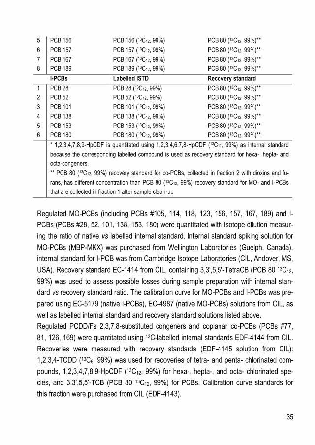
35
5 PCB 156 PCB 156 (13C12, 99%) PCB 80 (13C12, 99%)**
6 PCB 157 PCB 157 (13C12, 99%) PCB 80 (13C12, 99%)**
7 PCB 167 PCB 167 (13C12, 99%) PCB 80 (13C12, 99%)**
8 PCB 189 PCB 189 (13C12, 99%) PCB 80 (13C12, 99%)**
I-PCBs Labelled ISTD Recovery standard
1 PCB 28 PCB 28 (13C12, 99%) PCB 80 (13C12, 99%)**
2 PCB 52 PCB 52 (13C12, 99%) PCB 80 (13C12, 99%)**
3 PCB 101 PCB 101 (13C12, 99%) PCB 80 (13C12, 99%)**
4 PCB 138 PCB 138 (13C12, 99%) PCB 80 (13C12, 99%)**
5 PCB 153 PCB 153 (13C12, 99%) PCB 80 (13C12, 99%)**
6 PCB 180 PCB 180 (13C12, 99%) PCB 80 (13C12, 99%)**
* 1,2,3,4,7,8,9-HpCDF is quantitated using 1,2,3,4,6,7,8-HpCDF (13C12, 99%) as internal standard
because the corresponding labelled compound is used as recovery standard for hexa-, hepta- and
octa-congeners.
** PCB 80 (13C12, 99%) recovery standard for co-PCBs, collected in fraction 2 with dioxins and fu-
rans, has different concentration than PCB 80 (13C12, 99%) recovery standard for MO- and I-PCBs
that are collected in fraction 1 after sample clean-up
Regulated MO-PCBs (including PCBs #105, 114, 118, 123, 156, 157, 167, 189) and I-
PCBs (PCBs #28, 52, 101, 138, 153, 180) were quantitated with isotope dilution measur-
ing the ratio of native vs labelled internal standard. Internal standard spiking solution for
MO-PCBs (MBP-MKX) was purchased from Wellington Laboratories (Guelph, Canada),
internal standard for I-PCB was from Cambridge Isotope Laboratories (CIL, Andover, MS,
USA). Recovery standard EC-1414 from CIL, containing 3,3',5,5'-TetraCB (PCB 80 13C12,
99%) was used to assess possible losses during sample preparation with internal stan-
dard vs recovery standard ratio. The calibration curve for MO-PCBs and I-PCBs was pre-
pared using EC-5179 (native I-PCBs), EC-4987 (native MO-PCBs) solutions from CIL, as
well as labelled internal standard and recovery standard solutions listed above.
Regulated PCDD/Fs 2,3,7,8-substituted congeners and coplanar co-PCBs (PCBs #77,
81, 126, 169) were quantitated using 13C-labelled internal standards EDF-4144 from CIL.
Recoveries were measured with recovery standards (EDF-4145 solution from CIL):
1,2,3,4-TCDD (13C6, 99%) was used for recoveries of tetra- and penta- chlorinated com-
pounds, 1,2,3,4,7,8,9-HpCDF (13C12, 99%) for hexa-, hepta-, and octa- chlorinated spe-
cies, and 3,3’,5,5’-TCB (PCB 80 13C12, 99%) for PCBs. Calibration curve standards for
this fraction were purchased from CIL (EDF-4143).
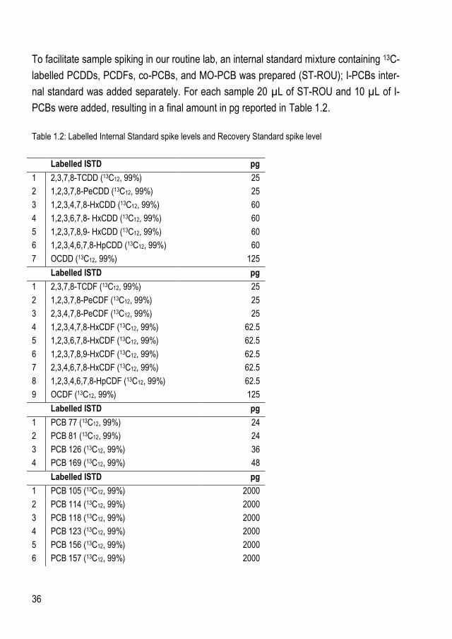
36
To facilitate sample spiking in our routine lab, an internal standard mixture containing 13C-
labelled PCDDs, PCDFs, co-PCBs, and MO-PCB was prepared (ST-ROU); I-PCBs inter-
nal standard was added separately. For each sample 20 µL of ST-ROU and 10 µL of I-
PCBs were added, resulting in a final amount in pg reported in Table 1.2.
Table 1.2: Labelled Internal Standard spike levels and Recovery Standard spike level
Labelled ISTD pg
1 2,3,7,8-TCDD (13C12, 99%) 25
2 1,2,3,7,8-PeCDD (13C12, 99%) 25
3 1,2,3,4,7,8-HxCDD (13C12, 99%) 60
4 1,2,3,6,7,8- HxCDD (13C12, 99%) 60
5 1,2,3,7,8,9- HxCDD (13C12, 99%) 60
6 1,2,3,4,6,7,8-HpCDD (13C12, 99%) 60
7 OCDD (13C12, 99%) 125
Labelled ISTD pg
1 2,3,7,8-TCDF (13C12, 99%) 25
2 1,2,3,7,8-PeCDF (13C12, 99%) 25
3 2,3,4,7,8-PeCDF (13C12, 99%) 25
4 1,2,3,4,7,8-HxCDF (13C12, 99%) 62.5
5 1,2,3,6,7,8-HxCDF (13C12, 99%) 62.5
6 1,2,3,7,8,9-HxCDF (13C12, 99%) 62.5
7 2,3,4,6,7,8-HxCDF (13C12, 99%) 62.5
8 1,2,3,4,6,7,8-HpCDF (13C12, 99%) 62.5
9 OCDF (13C12, 99%) 125
Labelled ISTD pg
1 PCB 77 (13C12, 99%) 24
2 PCB 81 (13C12, 99%) 24
3 PCB 126 (13C12, 99%) 36
4 PCB 169 (13C12, 99%) 48
Labelled ISTD pg
1 PCB 105 (13C12, 99%) 2000
2 PCB 114 (13C12, 99%) 2000
3 PCB 118 (13C12, 99%) 2000
4 PCB 123 (13C12, 99%) 2000
5 PCB 156 (13C12, 99%) 2000
6 PCB 157 (13C12, 99%) 2000

37
7 PCB 167 (13C12, 99%) 2000
8 PCB 189 (13C12, 99%) 2000
Labelled ISTD pg
1 PCB 28 (13C12, 99%) 2000
2 PCB 52 (13C12, 99%) 2000
3 PCB 101 (13C12, 99%) 2000
4 PCB 138 (13C12, 99%) 2000
5 PCB 153 (13C12, 99%) 2000
6 PCB 180 (13C12, 99%) 2000
Recovery standard pg
F1 PCB 80 (13C12, 99%) 2000
F2
1,2,3,4-TCDD (13C12, 99%) 12.5
1,2,3,4,7,8,9-HpCDF (13C12, 99%) 31.25
PCB 80 (13C12, 99%) for co-PCBs 24
4. Sample preparation for vegetable oil in our laboratory
As reported in the Introduction of this thesis, the experimental activity was carried out at
the University of Liège, at CART laboratory, that is a ISO 17025 accredited national refer-
ence laboratory for dioxin and PCB analysis. Sample preparation in this work of method
validation was done according to the validated method used for routine analysis.
For vegetable oil, sample preparation doesn’t include fat extraction as the matrix is al-
ready pure fat. Anyways sample clean-up is still indispensable in order to remove matrix
interferences, isolate and fractionate trace level dioxins from interfering chlorinated com-
pounds, PCB included. The procedure used is described in detail in Chapter 3, that re-
ports the development of alternative clean-up approaches based on our routine method.
Briefly, an aliquot of 4 grams of vegetable oil was weighted, diluted in 10 mL of hexane
and spiked with IS solution (20 µL of internal standard ST-ROU and 10 µL of I-PCBs so-
lution). Then the sample was directly cleaned-up according to our routine procedure that
includes a preliminary fat digestion with a manually packed acidic silica column, followed
by clean-up and fractionation with PowerPrepTM automated system from FMS (Fluid
Management System Inc.).

38
Preliminary lipid digestion was done with disposable glass column manually packed as
follows: (from the bottom) glass wool, 5 g Na2SO4, 5 g neutral silica, 20 g 44% acidic sil-
ica, 20 g 22% acidic silica. Hexane was used for column conditioning and elution. Col-
lected eluate was evaporated to approximately 10 mL before the introduction in Power-
PrepTM automated system for further clean-up and for fractionation of I- and MO-PCBs
(usually found at part-per-billion (ppb) level in food and feed) from PCDDs, PCDFs and
co-PCBs (usually found at part-per-trillion (ppt) level). PowerPrepTM system was equipped
with 3 column setup: standard multilayer silica column (4 g acidic, 2 g basic, 1.5 neutral),
basic alumina (11 g), carbon AX-21 column (0.34 g). Two fractions were collected out of
the system: fraction 1 (F1) eluted by forward elution of alumina/carbon column with a mix-
ture of hexane/dichloromethane 50/50 and containing I- and MO-PCBs; fraction 2 (F2)
collected by backflush elution of the carbon column with toluene and containing co-PCBs,
PCDFs and PCDDs. Solvent volumes were reduced to approximately 500 µL in dedi-
cated tubes using a sensor-equipped TurboVap II Workstation (Caliper Life Science,
Teraflene, Belgium), to be then transferred in GC vials containing nonane (90 µL for F1
and 4 µL F2) as keeper. Final evaporation for solvent exchange to nonane was done with
RapidVap (Labconco, Kansas City, MO, USA). Recovery standard was added to each
fraction before instrumental analysis to assess recoveries.
5. GC-MS/MS Triple Quad instrumental setup
For quantitative analysis, a 7000C GC-MS/MS Triple Quad system from Agilent (Palo
Alto, CA, USA) was used, according to a validated method developed in our laboratory
(L'Homme et al., 2015b). Briefly, the triple Quad instrument was equipped with a 7890B
GC oven, a programmable temperature vaporization (PTV) inlet, and a 7693A automated
liquid sampler (ALS). PTV inlet was operated in solvent vent mode and cooled by liquid
CO2; its temperature program was the same for both fractions F1 and F2 and was chosen
after an Experimental Design (DoE)(L'Homme et al., 2015a): start at 45°C (3 min) and
ramp at 720°C/min until 320°C; vent flow of 100 mL/min at pressure of 10 psi for 2.8 min.
Purge flow was set to 1200 mL/min after 5 min to avoid memory effect in the inlet. GC
column was the classic DB-5ms 60 m × 250 µm × 0.25 µm (Agilent). Injection volume
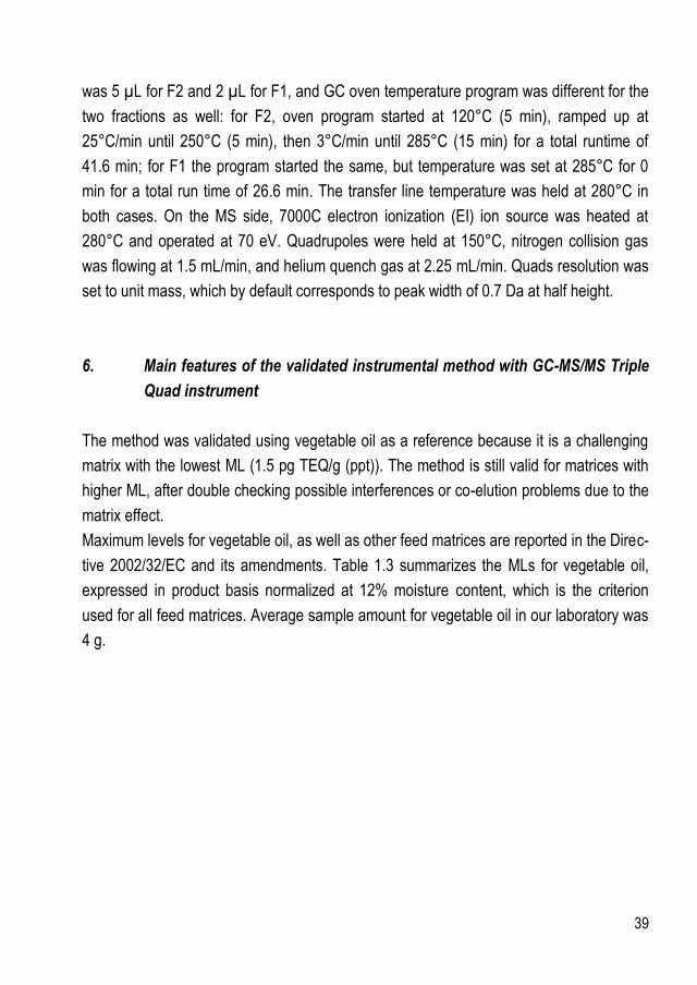
39
was 5 µL for F2 and 2 µL for F1, and GC oven temperature program was different for the
two fractions as well: for F2, oven program started at 120°C (5 min), ramped up at
25°C/min until 250°C (5 min), then 3°C/min until 285°C (15 min) for a total runtime of
41.6 min; for F1 the program started the same, but temperature was set at 285°C for 0
min for a total run time of 26.6 min. The transfer line temperature was held at 280°C in
both cases. On the MS side, 7000C electron ionization (EI) ion source was heated at
280°C and operated at 70 eV. Quadrupoles were held at 150°C, nitrogen collision gas
was flowing at 1.5 mL/min, and helium quench gas at 2.25 mL/min. Quads resolution was
set to unit mass, which by default corresponds to peak width of 0.7 Da at half height.
6. Main features of the validated instrumental method with GC-MS/MS Triple
Quad instrument
The method was validated using vegetable oil as a reference because it is a challenging
matrix with the lowest ML (1.5 pg TEQ/g (ppt)). The method is still valid for matrices with
higher ML, after double checking possible interferences or co-elution problems due to the
matrix effect.
Maximum levels for vegetable oil, as well as other feed matrices are reported in the Direc-
tive 2002/32/EC and its amendments. Table 1.3 summarizes the MLs for vegetable oil,
expressed in product basis normalized at 12% moisture content, which is the criterion
used for all feed matrices. Average sample amount for vegetable oil in our laboratory was
4 g.
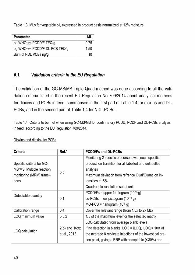
40
Table 1.3: MLs for vegetable oil, expressed in product basis normalized at 12% moisture.
Parameter ML
pg WHO2005-PCDD/F TEQ/g 0.75
pg WHO2005-PCDD/F-DL PCB TEQ/g 1.50
Sum of NDL PCBs ng/g 10
6.1. Validation criteria in the EU Regulation
The validation of the GC-MS/MS Triple Quad method was done according to all the vali-
dation criteria listed in the recent EU Regulation No 709/2014 about analytical methods
for dioxins and PCBs in feed, summarised in the first part of Table 1.4 for dioxins and DL-
PCBs, and in the second part of Table 1.4 for NDL-PCBs.
Table 1.4: Criteria to be met when using GC-MS/MS for confirmatory PCDD, PCDF and DL-PCBs analysis
in feed, according to the EU Regulation 709/2014.
Dioxins and dioxin-like PCBs
Criteria Ref.* PCDD/Fs and DL-PCBs
Specific criteria for GC-
MS/MS: Multiple reaction
monitoring (MRM) transi-
tions
6.5
Monitoring 2 specific precursors with each specific
product ion transition for all labelled and unlabelled
analytes
Maximum deviation from refrence Qual/Quant ion in-
tensities ±15%
Quadrupole resolution set at unit
Detectable quantity
5.1
PCDD/Fs = upper femtogram (10-15 g)
co-PCBs = low pictogram (10-12 g)
MO-PCB = nanogram (10-9 g)
Calibration range 6.4 Cover the relevant range (from 1/5x to 2x ML)
LOQ minimum value 5.5.2 1/5 of the maximum level for the selected matrix
LOQ calculation 2(b) and (Kotz
et al., 2012)
LOQ calculated from average blank levels
If no detection in blanks, LOQ = iLOQ, iLOQ = 10σ of
the average 8 replicate injections of the lowest calibra-
tion point, giving a RRF with acceptable (≤30%) and

41
consistent (RSD ≤ 15%) deviation to the ARRF
Acceptable difference be-
tween upper-bound and
lower-bound at maximum
level
6.1 Difference < 20%
Validation in the range of
the maximum level 5.4.1
Demonstrate performances at 0,5x, 1x, 2x with accept-
able RSDr (x = ML)
High selectivity (specificity) 5.2 and 6.3
Sample preparation has to separate PCDD/Fs from in-
terfering chlorinated compounds as NDL-PCBs and
polychlorinated diphenyl ethers;
Gas-chromatographic separation of 1,2,3,4,7,8-HxCDF
and 1,2,3,6,7,8-HxCDF, 25% peak to peak
High Accuracy (trueness
and precision) 5.3 and 5.6
Trueness: difference ±20% of certified value
Precision (RSDR) <15%
Blanks and QCs 5.4.2 Record control charts
Recovery check 6.2
Feed with fat content <10% ISTD added prior to extrac-
tion;
Recoveries in the range 60 to 120 % for each congener
Measurement Uncertainty 2.2 Expanded measurement uncertainty with cover factor 2
(95% level of confidence)
Reporting of results 8
x ± U (expanded measurement uncertainty)
results in the same units and the same significant fig-
ure as MLs set in the Regulation
* Ref.: number of the pertinent paragraph in the EU 709/2014
NDL-PCBs
Criteria Ref. NDL-PCB
Specific criteria for GC-
MS/MS: Multiple reaction
monitoring (MRM) transi-
tions
3.3 Monitor 1 precursor and 2 product ions
Tolerance ratio ±20% if rel. intens. >50%
Tolerance ratio ±25% if rel. intens. 20-50%
Quadrupole resolution set at unit
Detectable quantity
Calibration range
nanogram (10-9 g)
Calibration range 4 It has to include 0.5x and 2x the ML
LOQ minimum value 1/5 of the maximum level for the selected matrix
LOQ calculation
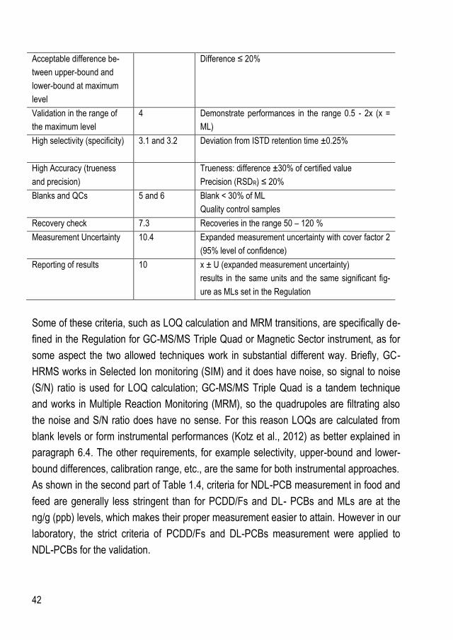
42
Acceptable difference be-
tween upper-bound and
lower-bound at maximum
level
Difference ≤ 20%
Validation in the range of
the maximum level
4 Demonstrate performances in the range 0.5 - 2x (x =
ML)
High selectivity (specificity) 3.1 and 3.2 Deviation from ISTD retention time ±0.25%
High Accuracy (trueness
and precision)
Trueness: difference ±30% of certified value
Precision (RSDR) ≤ 20%
Blanks and QCs 5 and 6 Blank < 30% of ML
Quality control samples
Recovery check 7.3 Recoveries in the range 50 – 120 %
Measurement Uncertainty 10.4 Expanded measurement uncertainty with cover factor 2
(95% level of confidence)
Reporting of results 10 x ± U (expanded measurement uncertainty)
results in the same units and the same significant fig-
ure as MLs set in the Regulation
Some of these criteria, such as LOQ calculation and MRM transitions, are specifically de-
fined in the Regulation for GC-MS/MS Triple Quad or Magnetic Sector instrument, as for
some aspect the two allowed techniques work in substantial different way. Briefly, GC-
HRMS works in Selected Ion monitoring (SIM) and it does have noise, so signal to noise
(S/N) ratio is used for LOQ calculation; GC-MS/MS Triple Quad is a tandem technique
and works in Multiple Reaction Monitoring (MRM), so the quadrupoles are filtrating also
the noise and S/N ratio does have no sense. For this reason LOQs are calculated from
blank levels or form instrumental performances (Kotz et al., 2012) as better explained in
paragraph 6.4. The other requirements, for example selectivity, upper-bound and lower-
bound differences, calibration range, etc., are the same for both instrumental approaches.
As shown in the second part of Table 1.4, criteria for NDL-PCB measurement in food and
feed are generally less stringent than for PCDD/Fs and DL- PCBs and MLs are at the
ng/g (ppb) levels, which makes their proper measurement easier to attain. However in our
laboratory, the strict criteria of PCDD/Fs and DL-PCBs measurement were applied to
NDL-PCBs for the validation.

43
6.2. MRM transitions
Measurements with GC-MS/MS Triple Quad were carried out in Multiple Reaction Moni-
toring (MRM) mode in tandem mass spectrometry. This is an important difference in com-
parison with the HR Magnetic Sector instrument that cannot work in MRM, but in Selected
Ion Monitoring (SIM). The EU Regulation reports specific criteria for GC-MS/MS and de-
mands to monitor, for each congener, two specific precursor ions with one specific prod-
uct ion (point 6.5 in the Regulation 709/2014). In our method, for the most toxic PCDD/Fs
and co-PCBs, three MRM transitions were followed, two for quantitation (‘Quant transi-
tions’) and one for qualification (‘Qual transition’) purposes. The two Quant transitions cor-
responded to the same precursor ion, for a total of two specific precursor ions and three
specific product ions for each congener, to prevent integration of interferences. The most
intense Quant transition was used for congener quantification as reported later. For MO-
and I-PCBs one Quant and one Qual transition were followed, for a total of two MRM
transitions as the minimum requirement of the EU Regulation. Table 1.5 shows Quant
and Qual transitions of all the congeners.
Tale 1.5: MRM Qual and Quant transitions recorded for all the congeners
PCDD congener Native Quant Native Qual Labelled Quant Labelled Qual
2,3,7,8-TCDD 319.9 -> 256.9, 258.9 321.9 -> 258.9 331.9 -> 267.9, 269.9 333.9 -> 269.9
1,2,3,7,8-PeCDD 355.9 -> 292.9, 290.9 353.9 -> 290.9 365.9 -> 301.9, 303.9 367.9 -> 303.9
1,2,3,4,7,8-HxCDD 389.8 -> 326.9, 328.8 391.8 -> 328.8 403.8 -> 339.8, 337.9 401.8 -> 337.9
1,2,3,6,7,8- HxCDD 389.8 -> 326.9, 328.8 391.8 -> 328.8 403.8 -> 339.8, 337.9 401.8 -> 337.9
1,2,3,7,8,9- HxCDD 389.8 -> 326.9, 328.8 391.8 -> 328.8 403.8 -> 339.8, 337.9 401.8 -> 337.9
1,2,3,4,6,7,8-HpCDD 423.8 -> 360.8, 362.8 425.8 -> 362.8 437.8 -> 373.8, 371.8 435.8 -> 371.8
OCDD 457.7 -> 394.8, 396.8 459.7 -> 396.8 469.7 -> 405.8, 407.8 471.7 -> 407.8
PCDF congener
2,3,7,8-TCDF 303.9 -> 240.9, 242.9 305.9 -> 242.9 315.9 -> 251.9, 253.9 317.9 -> 253.9
1,2,3,7,8-PeCDF 339.9 -> 276.9, 274.9 337.9 -> 274.9 351.9 -> 287.9, 285.9 349.9 -> 285.9
2,3,4,7,8-PeCDF 339.9 -> 276.9, 274.9 337.9 -> 274.9 351.9 -> 287.9, 285.9 349.9 -> 285.9
1,2,3,4,7,8-HxCDF 373.8 -> 310.9, 312.9 375.8 -> 312.9 385.8 -> 321.9, 323.9 387.8 -> 323.9
1,2,3,6,7,8-HxCDF 373.8 -> 310.9, 312.9 375.8 -> 312.9 385.8 -> 321.9, 323.9 387.8 -> 323.9
1,2,3,7,8,9-HxCDF 373.8 -> 310.9, 312.9 375.8 -> 312.9 385.8 -> 321.9, 323.9 387.8 -> 323.9
2,3,4,6,7,8-HxCDF 373.8 -> 310.9, 312.9 375.8 -> 312.9 385.8 -> 321.9, 323.9 387.8 -> 323.9

44
1,2,3,4,6,7,8-HpCDF 407.8 -> 344.8, 346.8 409.8 -> 346.8 419.8 -> 355.8, 357.88
421.8 -> 357.8
1,2,3,4,7,8,9-HpCDF 407.8 -> 344.8, 346.8 409.8 -> 346.8
OCDF 441.7 -> 378.8, 380.8 443.7 -> 380.8 453.7 -> 389.8, 391.8 455.7 -> 391.8
Co-PCBs
PCB 77 289.9 -> 219.9, 221.9 291.9 -> 221.9 301.9 -> 231.9, 233.9 303.9 -> 233.9
PCB 81 289.9 -> 219.9, 221.9 291.9 -> 221.9 301.9 -> 231.9, 233.9 303.9 -> 233.9
PCB 126 323.9 -> 253.9, 255.9 325.9 -> 255.9 335.9 -> 265.9, 267.9 337.9 -> 267.9
PCB 169 359.9 -> 289.9, 287.9 357.8 -> 287.9 371.9 -> 301.9, 299.9 369.9 -> 299.9
MO-PCBs
PCB 105 325.9 -> 255.9 327.9 -> 257.9 337.9 -> 267.9 339.9 -> 269.9
PCB 114 325.9 -> 255.9 327.9 -> 257.9 337.9 -> 267.9 339.9 -> 269.9
PCB 118 325.9 -> 255.9 327.9 -> 257.9 337.9 -> 267.9 339.9 -> 269.9
PCB 123 325.9 -> 255.9 327.9 -> 257.9 337.9 -> 267.9 339.9 -> 269.9
PCB 156 359.9 -> 289.9 361.9 -> 291.8 371.9 -> 301.9 373.9 -> 303.8
PCB 157 359.9 -> 289.9 361.9 -> 291.8 371.9 -> 301.9 373.9 -> 303.8
PCB 167 359.9 -> 289.9 361.9 -> 291.8 371.9 -> 301.9 373.9 -> 303.8
PCB 189 393.8 -> 323.8 395.8 -> 325.8 405.8 -> 335.8 407.8 -> 337.8
I-PCBs
PCB 28 256.0 -> 186.0 258.0 -> 188.0 268.0 -> 198.0 270.0 -> 200.0
PCB 52 289.9 -> 219.9 291.9 -> 221.9 301.9 -> 231.9 303.9 -> 233.9
PCB 101 325.9 -> 255.9 327.9 -> 257.9 337.9 -> 267.9 339.9 -> 269.9
PCB 138 359.9 -> 289.9 361.9 -> 291.8 371.9 -> 301.9 373.9 -> 303.8
CB 153 359.9 -> 289.9 361.9 -> 291.8 371.9 -> 301.9 373.9 -> 303.8
PCB 180 393.8 -> 323.8 395.8 -> 325.8 405.8 -> 335.8 407.8 -> 337.8
Recovery standard
1,2,3,4-TCDD
(13C6, 99%)
325.9 -> 262.9, 264.9 327.9 -> 264.9
1,2,3,4,7,8,9-HpCDF (13C12, 99%)
419.8 -> 355.8, 357.8 421.8 -> 357.8
PCB 80 (13C12, 99%) 301.9 -> 231.9, 233.9 303.9 -> 233.9
Peak area of the most intense Quant transition was used for congener quantitation, calcu-
lated through the ratio with the area of the corresponding labelled ISTD according to
Equation 1 of the Isotope Dilution (ID) technique. For all the calculations, chromatograms
without smoothing were used to stay as close as possible to raw data and to avoid any ar-
tificial effect on the signal and then congener quantification. The experimental ratio be-
tween Quant and Qual transition was monitored as well, to double check for interfer-
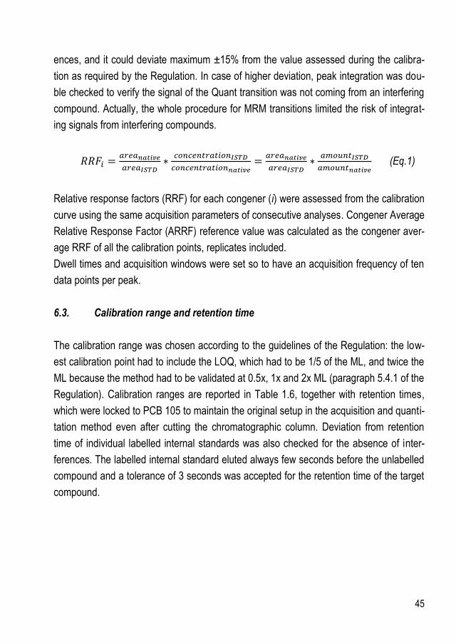
45
ences, and it could deviate maximum ±15% from the value assessed during the calibra-
tion as required by the Regulation. In case of higher deviation, peak integration was dou-
ble checked to verify the signal of the Quant transition was not coming from an interfering
compound. Actually, the whole procedure for MRM transitions limited the risk of integrat-
ing signals from interfering compounds.
(Eq.1)
Relative response factors (RRF) for each congener (i) were assessed from the calibration
curve using the same acquisition parameters of consecutive analyses. Congener Average
Relative Response Factor (ARRF) reference value was calculated as the congener aver-
age RRF of all the calibration points, replicates included.
Dwell times and acquisition windows were set so to have an acquisition frequency of ten
data points per peak.
6.3. Calibration range and retention time
The calibration range was chosen according to the guidelines of the Regulation: the low-
est calibration point had to include the LOQ, which had to be 1/5 of the ML, and twice the
ML because the method had to be validated at 0.5x, 1x and 2x ML (paragraph 5.4.1 of the
Regulation). Calibration ranges are reported in Table 1.6, together with retention times,
which were locked to PCB 105 to maintain the original setup in the acquisition and quanti-
tation method even after cutting the chromatographic column. Deviation from retention
time of individual labelled internal standards was also checked for the absence of inter-
ferences. The labelled internal standard eluted always few seconds before the unlabelled
compound and a tolerance of 3 seconds was accepted for the retention time of the target
compound.

46
Table 1.6: Calibration ranges for all the congeners
PCDDs Retention time
min
Lowest cali point
pg/µL
Highest cali point
pg/µL
2,3,7,8-TCDD 20.72 0.016 0.800
1,2,3,7,8-PeCDD 24.31 0.016 0.800
1,2,3,4,7,8-HxCDD 27.97 0.016 0.800
1,2,3,6,7,8- HxCDD 28.10 0.040 2.000
1,2,3,7,8,9- HxCDD 28.46 0.080 4.000
1,2,3,4,6,7,8-HpCDD 32.93 0.400 10.000
OCDD 39.35 4.000 120.000
PCDFs
2,3,7,8-TCDF 20.30 0.016 0.800
1,2,3,7,8-PeCDF 23.26 0.016 0.800
2,3,4,7,8-PeCDF 24.06 0.016 0.800
1,2,3,4,7,8-HxCDF 27.02 0.016 0.800
1,2,3,6,7,8-HxCDF 27.15 0.016 0.800
1,2,3,7,8,9-HxCDF 27.79 0.016 0.800
2,3,4,6,7,8-HxCDF 28.94 0.016 0.800
1,2,3,4,6,7,8-HpCDF 31.09 0.080 4.000
1,2,3,4,7,8,9-HpCDF 33.92 0.016 0.800
OCDF 39.76 0.016 0.800
Co-PCBs
PCB 77 17.71 0.320 8.000
PCB 81 18.02 0.320 8.000
PCB 126 20.92 0.320 8.000
PCB 169 24.17 0.320 8.000
MO-PCBs
PCB 105 19.66 1.000 80.000
PCB 114 19.12 1.000 80.000
PCB 118 18.74 1.000 80.000
PCB 123 18.62 1.000 80.000
PCB 156 22.51 1.000 80.000
PCB 157 22.71 1.000 80.000
PCB 167 21.56 1.000 80.000
PCB 189 25.76 1.000 80.000
I-PCBs
PCB 28 14.19 4.000 1000.000

47
PCB 52 14.79 4.000 1000.000
PCB 101 16.81 4.000 1000.000
PCB 138 20.46 4.000 1000.000
PCB 153 19.43 4.000 1000.000
PCB 180 23.14 4.000 80.000
6.4. Limit of Quantitation (LOQ) and detectable quantity
The proper establishment of the limit of quantitation (LOQ) is one of the major differences
between the GC-HRMS method and the GC-MS/MS Triple Quad method. In GC-HRMS,
LOQs are calculated from S/N (signal/noise) ratio, but this cannot be calculated on the
GC-MS/MS Triple Quad because the two quadrupoles working in tandem are filtering
ions, with the effect of deeply reducing also the noise and making S/N calculation mean-
ingless. The EU Regulation 709/2014, at point 2, reports a definition of the LOQ for GC-
MS/MS instruments, but it does not explain precisely how to calculate it. Such a definition
of the LOQ can lead to several interpretation and way of calculation. This is undesirable
as improper establishment of LOQs of individual congeners might lead to inaccurate final
result calculations and inaccurate method performances estimation.
In our laboratory LOQ was calculated first from the levels of each congener in procedural
blanks. As reported in the Regulation, procedural blank analysis shall be performed by
carrying out the entire analytical procedure, omitting only the sample. Hence, for vegeta-
ble oil the blank consisted of 10 mL of hexane spiked with IS solutions and processed as
the matrix.
For LOQ assessment, 12 procedural blanks were prepared and analysed. For each con-
gener, the average level (in absolute amount, pg) and the standard deviation (s) were
calculated. Specific congener LOQ was calculated as the average value plus 6 times s
(Equation 2); doing so, whenever an experimental signal is higher than LOQ, it is statisti-
cally coming from the sample and not from the background.
(Eq. 2)
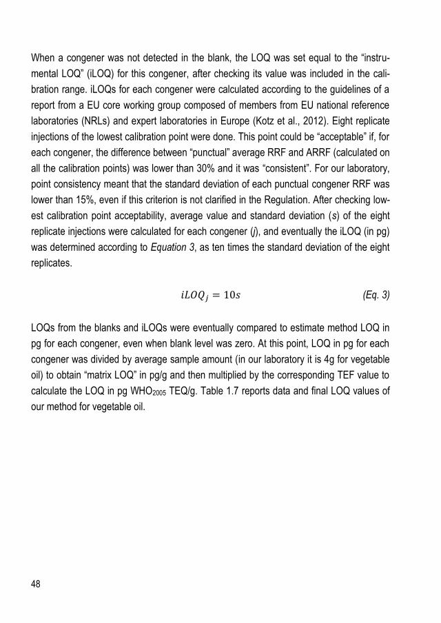
48
When a congener was not detected in the blank, the LOQ was set equal to the “instru-
mental LOQ” (iLOQ) for this congener, after checking its value was included in the cali-
bration range. iLOQs for each congener were calculated according to the guidelines of a
report from a EU core working group composed of members from EU national reference
laboratories (NRLs) and expert laboratories in Europe (Kotz et al., 2012). Eight replicate
injections of the lowest calibration point were done. This point could be “acceptable” if, for
each congener, the difference between “punctual” average RRF and ARRF (calculated on
all the calibration points) was lower than 30% and it was “consistent”. For our laboratory,
point consistency meant that the standard deviation of each punctual congener RRF was
lower than 15%, even if this criterion is not clarified in the Regulation. After checking low-
est calibration point acceptability, average value and standard deviation (s) of the eight
replicate injections were calculated for each congener (j), and eventually the iLOQ (in pg)
was determined according to Equation 3, as ten times the standard deviation of the eight
replicates.
(Eq. 3)
LOQs from the blanks and iLOQs were eventually compared to estimate method LOQ in
pg for each congener, even when blank level was zero. At this point, LOQ in pg for each
congener was divided by average sample amount (in our laboratory it is 4g for vegetable
oil) to obtain “matrix LOQ” in pg/g and then multiplied by the corresponding TEF value to
calculate the LOQ in pg WHO2005 TEQ/g. Table 1.7 reports data and final LOQ values of
our method for vegetable oil.

49
Table 1.7: Average blank levels and corresponding standard deviation for 12 blanks, derived LOQ calcula-
tion, iLOQ, and final vegetable oil LOQs in pg/g fat and in pg TEQ/g fat. Vegetable oil sample amount was 4
g.
PCDDs Average
blk
pg
SD
blk
pg
LOQ
pg
iLOQ
pg
Matrix LOQ
pg/g
Matrix LOQ
pg WHO2005TEQ/g
2,3,7,8-TCDD 0.000 0.000 0.000 0.017 0.004 0.004
1,2,3,7,8-PeCDD 0.000 0.000 0.000 0.033 0.008 0.008
1,2,3,4,7,8-HxCDD 0.000 0.000 0.000 0.027 0.007 0.001
1,2,3,6,7,8- HxCDD 0.043 0.083 0.543 0.033 0.136 0.014
1,2,3,7,8,9- HxCDD 0.007 0.021 0.130 0.071 0.033 0.003
1,2,3,4,6,7,8-HpCDD 0.403 0.259 1.959 0.056 0.490 0.005
OCDD 1.910 1.094 8.477 0.464 2.119 0.001
Sum LOQs PCDD 0.036
PCDFs
2,3,7,8-TCDF 0.043 0.067 0.442 0.052 0.111 0.011
1,2,3,7,8-PeCDF 0.566 0.309 2.420 0.021 0.605 0.018
2,3,4,7,8-PeCDF 0.015 0.052 0.327 0.021 0.082 0.025
1,2,3,4,7,8-HxCDF 0.018 0.045 0.288 0.016 0.072 0.007
1,2,3,6,7,8-HxCDF 0.018 0.037 0.240 0.021 0.060 0.006
1,2,3,7,8,9-HxCDF 0.050 0.112 0.722 0.024 0.181 0.018
2,3,4,6,7,8-HxCDF 0.027 0.047 0.311 0.015 0.078 0.008
1,2,3,4,6,7,8-HpCDF 0.504 0.266 2.101 0.053 0.525 0.005
1,2,3,4,7,8,9-HpCDF 0.005 0.011 0.069 0.048 0.017 0.000
OCDF 0.275 0.355 2.407 0.070 0.602 0.000
Sum LOQs PCDF 0.098
TOTAL LOQ (pg WHO2005 TEQ/g) dioxins 0.134
Co-PCBs
PCB 77 59.038 26.790 219.776 0.037 54.944 0.005
PCB 81 2.328 2.095 14.898 0.030 3.725 0.001
PCB 126 1.387 0.519 5.829 0.077 1.457 0.112
PCB 169 0.000 0.000 0.000 0.071 0.018 0.001
Sum LOQs Co-PCBs 0.119
MO-PCBs
PCB 105 282.561 166.864 1283.747 2.109 320.937 0.010
PCB 114 25.376 13.189 104.508 1.504 26.127 0.001
PCB 118 947.212 526.532 4106.404 1.930 826.601 0.027
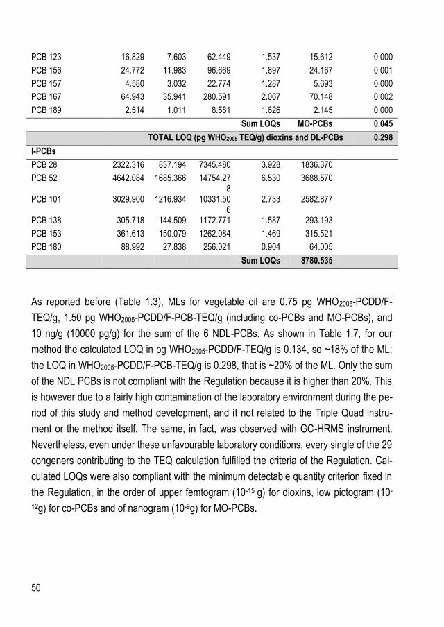
50
PCB 123 16.829 7.603 62.449 1.537 15.612 0.000
PCB 156 24.772 11.983 96.669 1.897 24.167 0.001
PCB 157 4.580 3.032 22.774 1.287 5.693 0.000
PCB 167 64.943 35.941 280.591 2.067 70.148 0.002
PCB 189 2.514 1.011 8.581 1.626 2.145 0.000
Sum LOQs MO-PCBs 0.045
TOTAL LOQ (pg WHO2005 TEQ/g) dioxins and DL-PCBs 0.298
I-PCBs
PCB 28 2322.316 837.194 7345.480 3.928 1836.370
PCB 52 4642.084 1685.366 14754.278
6.530 3688.570
PCB 101 3029.900 1216.934 10331.506
2.733 2582.877
PCB 138 305.718 144.509 1172.771 1.587 293.193
PCB 153 361.613 150.079 1262.084 1.469 315.521
PCB 180 88.992 27.838 256.021 0.904 64.005
Sum LOQs 8780.535
As reported before (Table 1.3), MLs for vegetable oil are 0.75 pg WHO2005-PCDD/F-
TEQ/g, 1.50 pg WHO2005-PCDD/F-PCB-TEQ/g (including co-PCBs and MO-PCBs), and
10 ng/g (10000 pg/g) for the sum of the 6 NDL-PCBs. As shown in Table 1.7, for our
method the calculated LOQ in pg WHO2005-PCDD/F-TEQ/g is 0.134, so ~18% of the ML;
the LOQ in WHO2005-PCDD/F-PCB-TEQ/g is 0.298, that is ~20% of the ML. Only the sum
of the NDL PCBs is not compliant with the Regulation because it is higher than 20%. This
is however due to a fairly high contamination of the laboratory environment during the pe-
riod of this study and method development, and it not related to the Triple Quad instru-
ment or the method itself. The same, in fact, was observed with GC-HRMS instrument.
Nevertheless, even under these unfavourable laboratory conditions, every single of the 29
congeners contributing to the TEQ calculation fulfilled the criteria of the Regulation. Cal-
culated LOQs were also compliant with the minimum detectable quantity criterion fixed in
the Regulation, in the order of upper femtogram (10-15 g) for dioxins, low pictogram (10-
12g) for co-PCBs and of nanogram (10-9g) for MO-PCBs.

51
As already reported, the LOQ is a crucial parameter because of the reporting system of
the final results, as LOQ is the threshold values used to determine upper-bound, medium-
bound, and lower-bound values. The lower, medium and upper bound approaches consist
in reporting respectively zero, LOQ/2 and LOQ whenever the measured level is below the
LOQ for a target compound. The value calculated with the upper bound approach is used
to check for sample compliance to MLs, and this is the reason why LOQ calculation is
crucial in dioxin analysis.
6.5. Selectivity
Criteria for selectivity in the Regulation are the same if working with HRMS or Triple Quad
instruments. Peaks relative to 1,2,3,4,7,8- and 1,2,3,6,7,8-hexachlorinated furans conge-
ners (HxCDFs) have to show maximum 25% overlapping. Chromatographic separation of
other peaks is ensured when this criterion is fulfilled. In the method developed, these two
congeners were baseline separated (Figure 1.1)
Figure 1.1: Chromatogram of the two heptafurans, showing their clear separation (non-smoothed signals).
1,2,3,4,6,7,8-HpCDF RT=31.084 min
1,2,3,4, 7,8,9-HpCDF RT=33.898
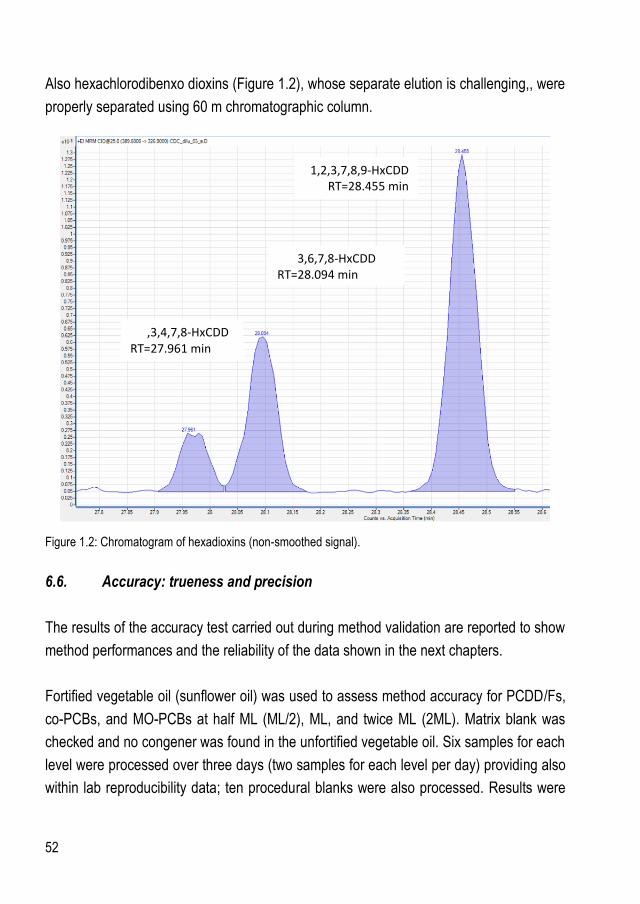
52
Also hexachlorodibenxo dioxins (Figure 1.2), whose separate elution is challenging,, were
properly separated using 60 m chromatographic column.
Figure 1.2: Chromatogram of hexadioxins (non-smoothed signal).
6.6. Accuracy: trueness and precision
The results of the accuracy test carried out during method validation are reported to show
method performances and the reliability of the data shown in the next chapters.
Fortified vegetable oil (sunflower oil) was used to assess method accuracy for PCDD/Fs,
co-PCBs, and MO-PCBs at half ML (ML/2), ML, and twice ML (2ML). Matrix blank was
checked and no congener was found in the unfortified vegetable oil. Six samples for each
level were processed over three days (two samples for each level per day) providing also
within lab reproducibility data; ten procedural blanks were also processed. Results were
1,2,3,4,7,8-HxCDD RT=27.961 min
1,2,3,7,8,9-HxCDD RT=28.455 min
1,2,3,6,7,8-HxCDD RT=28.094 min

53
obtained and reported by independent operators who operated without knowing target
levels. Table 1.8 shows the results of the accuracy experiments.
Table 1.8: Results of the accuracy test.
Experimental value
pg WHO2005 TEQ/g
SD
pg WHO2005 TEQ/g
RDS
%
Target value
pg WHO2005 TEQ/g
Bias
%
PCDD/Fs
ML/2 0.41 0.03 7.1 0.40 2.36
ML 0.78 0.04 5.7 0.79 -1.54
2ML 1.60 0.03 2.2 1.58 1.30
DL-PCBs
0.31 0.03 9.0 0.33 -7.00
0.59 0.02 3.4 0.65 -8.53
1.26 0.02 1.6 1.30 -3.42
These results met the EU Regulation criteria, that set the bias <20% and within lab repro-
ducibility <15%. The method, then, showed to be accurate and reliable.
7. Conclusions
This chapter described the GC-MS/MS Triple Quad acquisition method for dioxin and
PCB analysis used in this work of thesis. When this work of thesis was done, the method
was already developed and validated for vegetable oil, but in this work, the GC-MS/MS
method was optimized in some parameters, because it was applied to matrices other than
vegetable oil. In fact, it was used for the assessment of levels and recoveries in the next
chapters, which report the development of alternative clean-up approaches using auto-
mated systems, as well as the development of an analytical method for Dechlorane de-
tection in food and feed samples. Quantitative analysis was performed mainly with GC-
MS/MS Triple Quad to determine recovery rates, as well as levels in QC samples (pork,
milk and egg), with the aim of evaluating the suitability of the new clean-up strategy pro-
posed.

54
Moreover, this GC-MS/MS acquisition method was used for the first time in our labora-
tory, for Dechlorane detection in food and feed, which in general is a novelty because
usually Dechloranes are usually detected with GC-HRMS instruments.
55
Bibliography
BEHNISCH P.A., ALLEN, R., ANDERSON, J., BROUWER, A., BROWN, D., CAMPBELL, T., GOEYENS, L., HARRISON, R., HOOGENBOOM, R., VAN OVERMEIRE, I., TRAAG, W. & MALISCH, R. 2001. Harmonised Quality Criteria for Chemical and Bioassays Analyses of PCDDs/PCDFs in Feed and Food. Part 2: General Considerations, Bioassay Methods. Organohalogen Compounds.
EC 2002. DIRECTIVE 2002/32/EC OF THE EUROPEAN PARLIAMENT AND OF THE COUNCIL of 7 May 2002 on undesirable substances in animal feed.
EC 2014a. COMMISSION REGULATION (EU) No 589/2014 of 2 June 2014 laying down methods of sampling and analysis for the control of levels of dioxins, dioxin-like PCBs and non-dioxin-like PCBs in certain foodstuffs and repealing Regulation (EU) No 252/2012. In: COMMISSION, E. (ed.).
EC 2014b. COMMISSION REGULATION (EU) No 709/2014 of 20 June 2014 amending Regulation (EC) No 152/2009 as regards the determination of the levels of dioxins and polychlorinated biphenyls. In: COMMISSION, E. (ed.).
EPPE, G., GIANFRANCO DILETTI, ALWYN FERNANDES, JOHANNES HAEDRICH, JERRY HART, HELGE HOVE, ANNA LAURA IAMICELI, ALEXANDER KOTZ, RAINER MALISCH, MARCHAND, P., WOLFGANG MOCHE, GEORGES SCHOLL, GIAMPIERO SCORTICHINI, THORSTEN BERNSMANN, YVES TONDEUR & TRAAG, W. 2014. MEASUREMENT UNCERTAINTY FOR PERSITENT ORGANIC POLLUTANTS BY ISOTOPE-DILUTION MASS SPECTROMETRY. Organohalogen Compounds, 76, 4.
FOCANT, J. F. & EPPE, G. 2013. 3 - Screening and confirmatory methods for the detection of dioxins and polychlorinated biphenyls (PCBs) in foods. In: ROSE, M. & FERNANDES, A. (eds.) Persistent Organic Pollutants and Toxic Metals in Foods. Woodhead Publishing.
FOCANT, J. F., PIRARD, C., EPPE, G. & DE PAUW, E. 2005. Recent advances in mass spectrometric measurement of dioxins. Journal of Chromatography A, 1067, 265-275.
GARCÍA-BERMEJO, Á., ÁBALOS, M., SAULÓ, J., ABAD, E., GONZÁLEZ, M. J. & GÓMARA, B. 2015. Triple quadrupole tandem mass spectrometry: A real alternative to high resolution magnetic sector instrument for the analysis of polychlorinated dibenzo-p-dioxins, furans and dioxin-like polychlorinated biphenyls. Analytica Chimica Acta, 889, 156-165.
INGELIDO, A. M., BRAMBILLA, G., ABBALLE, A., DI DOMENICO, A., FULGENZI, A. R., IACOVELLA, N., VALENTINI, A. L. I. S. & FELIP, E. D. 2012. PCDD, PCDF, and DL-PCB analysis in food: Performance evaluation of the high-resolution gas chromatography/low-resolution tandem mass spectrometry technique using

56
consensus-based samples. Rapid Communications in Mass Spectrometry, 26, 236-242.
KOTZ A, MALISCH R, WAHL K, BITOMSKY N, ADAMOVIC K, GERTEISEN I, LESWAL S, SCHACHTELE J, TRITSCHLER R & H, W. 2011. GC-MS/MS Determination of PCDD/Fs and PCBs in Feed and Food- Comparison With GC-HRMS. Organohalogen Compounds, 73, 4.
KOTZ, A., MALISCH, R., FOCANT, J., EPPE, G., CEDERBERG, T., RANTAKOKKO, P., FURST, P., BERNSMANN, T., LEONDIADIS, L., LOVASZ, C., SCORTICHINI, G., DILETTI, G., DI DOMENICO, A., INGELIDO, A., TRAAG, W., SMITH, F. & FERNANDES, A. 2012. Analytical criteria for use of MS/MS for determination of dioxins and dioxin-like PCBs in feed and food. Organohalogen Compounds, 74, 4.
L'HOMME, B., CALAPRICE, C., CALVANO, C. D., ZAMBONIN, C., LEARDI, R. & FOCANT, J. F. 2015a. Ultra-trace measurement of Dechloranes to investigate food as a route of human exposure. Chemosphere, 139, 525-533.
L'HOMME, B., SCHOLL, G., EPPE, G. & FOCANT, J. F. 2015b. Validation of a gas chromatography-triple quadrupole mass spectrometry method for confirmatory analysis of dioxins and dioxin-like polychlorobiphenyls in feed following new EU Regulation 709/2014. Journal of Chromatography A, 1376, 149-158.
MALISCH R., BERT BAUMANN, PETER A. BEHNISCH, RICHARD CANADY, DANIEL FRAISSE, PETER FURST, DOUGLAS HAYWARD, RONALD HOOGENBOOM, RONALD HOOGERBRUGGE, DJIEN LIEM, PSPKE, O., WIM TRAAG & WIESMULLER', T. 2001. Harminised quality criteria for chemical and bioassayes of PCDDs/PCDFs in feed and food. Part 1: general considerations, GC/MS methods. Organohalogen Compounds, 50.
REINER, E. J., CLEMENT, R. E., OKEY, A. B. & MARVIN, C. H. 2006. Advances in analytical techniques for polychlorinated dibenzo-p-dioxins, polychlorinated dibenzofurans and dioxin-like PCBs. Analytical and Bioanalytical Chemistry, 386, 791-806.
SANDY C, FURST P, BERNSMANN T & D, B. 2011. Determination of Polychlorinated Biphenyl Congeners in Foodstuffs and Animal Feed Using a Triple Quadrupole GC-MS/MS Instrument. Organohalogen Compounds, 73, 4.

57
CHAPTER II
Development of a new dioxin/PCB clean-up and fractionation procedure
for an existing automated system
1. Introduction
Polychlorinated dibenzo-p-dioxins (PCDDs), polychlorinated dibenzofurans (PCDFs) and
polychlorinated biphenyls (PCBs), have been recognised as highly toxic and ubiquitous
environmental contaminants. The most toxic congeners of these three organochlorine
families are PCDDs and PCDFs with chlorine in the 2,3,7,8-positions, the planar CBs
(non-ortho substituted), and semiplanar (mono-ortho and di-ortho substituted) (Safe,
1990). The determination of these individual congeners in food and feed samples involves
sophisticated and delicate multistage sample preparation because of the extremely low
concentrations of PCDD/PCDFs and co-PCBs (part per trillion, ppt) and the presence of
many other co-extracted and more concentrate organic compounds, such as lipids. For
this reason, after fat extraction, a clean-up step is of prime importance and is aimed to the
elimination of these co-extracted analytes and to the separation of some PCBs and diox-
ins to avoid successive interferences during instrumental quantification. In addition to the
clean-up procedure, high-resolution gas chromatography (HRGC) coupled with high-
resolution mass spectrometry (HRMS) is essential for the accurate and specific determi-
nation of these compounds, characterised by structure-related toxicity and a great num-
ber of congeners. Recently Triple Quadrupole low resolution (LR)MS instruments have
shown performances that demonstrate their suitability for confirmatory analysis, recog-
nized by EU Regulation (2014a, 2014b).
Most of the clean-up methods described in the literature are based on more than one col-
umn-chromatographic step and are therefore very time and solvent consuming. Mainly,
clean-up methods are based on lipid oxidation via sulfuric acid coated silica gel column,
PCBs and PCDD/Fs fractionation by means of Florisil® or alumina column, and eventually
activated charcoal to complete fractionation and isolate planar compounds because of
geometric interaction with the planar structure of the carbon. Adopted sorbents affect final
58
fractionation profile, also related to instrumental acquisition method: usually 2 fractions
per sample are collected in the end of the sample preparation, but some laboratories frac-
tionate up to 4 fractions; then, based on the fractionation profile, 2 or more chroma-
tographic runs are carried out for quantification. Many routine laboratories collect and
quantify 2 fractions containing I- and MO-PCBs together and co-PCBs, PCDFs and
PCDDs separately, because their average levels in real food and feed samples are in the
part per billion (ppb) range, 1000 times higher than average levels of co-PCBs, PCDDs,
and PCDFs that are found at ppt level and quantified in a separate GC-MS run. For some
laboratories, separate quantification of mono- and di-ortho PCBs from co-PCBs is impor-
tant also because PCB 126 and 169, with the highest TEFs among PCBs, can be subject
to instrumental interferences from other PCBs with possible overestimation (Bernsmann
T. et al., 2014). Other laboratories regularly collect and analyse 2 fractions with different
composition: all the PCBs (I-, MO- and co-PCBs) are collected in the same fraction and
PCDD/Fs are separate, with no instrumental quantification issue (Aries et al., 2004, Fürst,
2006).Some other laboratories are further splitting co-PCBs from PCDD/Fs, collecting 4
fractions per sample, namely I-PCBS, MO-PCBs, co-PCBS and PCDD/Fs, and doing 3 in-
jections, one for I- and MO-PCBs, one for co-PCBs and one for PCDD/Fs. This is be-
cause PCB 126 and 169 have retention time very close to 2,3,7,8 TCDD and 1,2,3,7,8
PeCDD respectively (difference around 0.2 min depending on chromatographic setup)
with quantification issues if the level of co-PCBs is higher than dioxins one for the same
samples
The goal of the present work was to develop new and high throughput clean-up ap-
proaches for an existing automated system, the DEXTechTM from LCTech GmbH. The
new strategies were based on silica and carbon columns commercially available for
DEXTechTM system, and on manually packed alumina column prepared in our laboratory.
The two methods lead to different final fractionation profiles due to the use of different
carbon sorbents after the fractionation with alumina. New methods showed a great im-
provement in terms of solvent and time saving in comparison with the classic clean-up
method routinely used for the same system.
59
2. Materials and methods
2.1. Chemicals and consumables
Solvents (hexane, dichloromethane, toluene) were Picograde® reagents (LGC Promo-
chem, Wesel, Germany). All solvent batches were tested for investigated analyte con-
tamination before use. Nonane and dodecane puriss analytical-reagent grade standard
for GC were purchased from Fluka (Steinheim, Germany). Water was obtained from a
Milli-Q Ultrapure water purification system (Millipore, Brussels, Belgium). Ethanol, ammo-
nium hydroxide solution 28-30% and ethyl ether were purchased from Sigma Aldrich (St.
Louis, MO, USA). Sodium sulphate and diatomaceous earth were purchased from VWR
International (Radnor, PA, USA). Neutral and basic aluminium oxides were purchased
from Sigma-Aldrich. Disposable multilayer silica and carbon columns for the automated
clean-up DEXTechTM system were obtained from LCTech (LCTech GmbH, Dorfen, Ger-
many).
Ten mL glass syringes from Microsyringes (ILS Innovative Labor Systeme GmbH, Stütz-
erbach, Germany) and/or sterile disposable plastic syringes from B. Braun (Melsungen,
Germany) were used for injection. Chromatographic pure grade helium gas, 99.9999%
alphagaz 2 was purchased from Air Liquide (Paris, France). Technical N27 grade liquid
CO2 was used for PTV cooling (Air Liquide, Paris, France).
In our accredited ISO 17025 routine laboratory, in dioxin analysis after all the analytical
procedure, two fractions are collected and injected for instrumental quantification: one
containing I- and MO-PCBs, and one containing co-PCBs, PCDFs and PCDDs. Regu-
lated MO-PCBs (including PCBs #105, 114, 118, 123, 156, 157, 167, 189) and I-PCBs
(PCBs #28, 52, 101, 138, 153, 180) were quantitated with isotope dilution measuring the
ratio of native vs labelled internal standard. Internal standard spiking solution for MO-
PCBs (MBP-MKX) was purchased from Wellington Laboratories (Guelph, Canada), inter-
nal standard for I-PCB was from Cambridge Isotope Laboratories (CIL, Andover, MS,
USA). Recovery standard EC-1414 from CIL, containing 3,3',5,5'-TetraCB (PCB 80)
(13C12, 99%) was used to assess possible losses during sample preparation with internal
standard vs recovery standard ratio. The calibration curve for MO-PCBs and I-PCBs was

60
prepared using EC-5179 (native I-PCBs), EC-4987 (native MO-PCBs) solutions from CIL,
listed above internal standard solutions and recovery standard solutions.
Regulated PCDD/Fs 2,3,7,8-substituted congeners and coplanar co-PCBs (PCBs #77,
81, 126, 169) were quantitated using 13C-labelled internal standards EDF-4144 from CIL.
Recoveries were measured with recovery standards (EDF-4145 solution from CIL):
1,2,3,4-TCDD (13C6, 99%) was used for recoveries of tetra and penta chlorinated com-
pounds, 1,2,3,4,7,8,9-HpCDF (13C12, 99%) for hexa, hepta, and octa chlorinated species,
and 3,3’,5,5’-TCB (13C12 PCB 80, 99%) for PCBs. Calibration curve standards for this frac-
tion were purchased from CIL (EDF-4143).
To facilitate samples spiking in our routine lab, an internal standard mixture containing
13C-labelled PCDDs, PCDFs, co-PCBs, and MO-PCB was prepared (ST-ROU); I-PCBs
internal standard was added separately. 20 µL of ST-ROU and 10 µL of I-PCBs solution
are called labelled IS solution trough this work.
2.2. Sample preparation
During the first part of this work, model samples, consisting of 2 mL of hexane spiked with
IS solution (20 µL of internal standard ST-ROU and 10 µL of I-PCBs solution), were used
for method development. Model samples were directly injected in the clean-up system
with no preliminary sample preparation step, to assess recovery rates related to this part
of the analysis only. After method development, one of the two methods was applied to
quality control (QC) samples, consisting of pork fat (QCG), freeze-dried egg yolk (QCE),
and milk (QCL) to evaluate method performances on real fatty food matrices. Procedural
blanks were analysed in the same series of corresponding QCs and were respectively
pure hexane for pork fat, diatomaceous heart for egg yolks and ultrapure water for milk.
Normally if sample is not already pure fat, the first step of a dioxin analysis is fat extrac-
tion because dioxins are lipophilic compounds. In considered QCs, fat extraction was not
necessary only for pork fat, accelerated solvent extraction (ASETM 350, Dionex, Thermo
Fisher Scientific) was used for egg yolks, and liquid-liquid extraction was used for milk.
For pork fat, 5 g were directly diluted in hexane and spiked with labelled IS before sample
clean-up.

61
For egg yolk, 5 g of freeze-dried sample were first mixed with diatomaceous heart and
then extracted with ASE system and solvent toluene/ethanol 90/10 at 150°C for 5 minutes
for 2 cycles. Extracts were filtrated over Na2SO4 and solvent was evaporated until dry-
ness for fat determination. The extracted fat, approximately 2.5 g, was spiked with la-
belled IS solutions prior introduction in the clean-up system. Diatomaceous earth was
used as blank and followed the same procedure.
For QC milk samples, liquid-liquid extraction was carried out: 80 mL were poured in a
separation funnel, 20 mL of NH3 and 80 mL of ethanol were added, the funnel was
shaken and 100 mL of ethyl ether was added and the solution was left for 30 minutes to
allow separation of the two phases; eventually hexane was added and left 30 minutes un-
til the clear separation of aqueous and organic phase. This latter was transferred in a
round flask for gravimetric determination of fat content, which was spiked with labelled IS
solutions after solvent evaporation. The blank was 80 mL MQ ultrapure water following
the same procedure as the sample.
Samples were injected in the DEXTechTM automated system for clean-up using the pro-
cedure with basic alumina described in the following sections.
2.2.1. DEXTechTM system for sample clean-up
The aim of this work was to develop an alternative approach for sample clean-up using an
already existing automated system, DEXTechTM from LCTech GmbH (Figure 2.1).
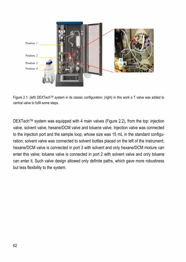
62
Figure 2.1: (left) DEXTechTM system in its classic configuration; (right) in this work a T valve was added to
central valve to fulfil some steps.
DEXTechTM system was equipped with 4 main valves (Figure 2.2), from the top: injection
valve, solvent valve, hexane/DCM valve and toluene valve. Injection valve was connected
to the injection port and the sample loop, whose size was 15 mL in the standard configu-
ration; solvent valve was connected to solvent bottles placed on the left of the instrument;
hexane/DCM valve is connected in port 3 with solvent and only hexane/DCM mixture can
enter this valve; toluene valve is connected in port 2 with solvent valve and only toluene
can enter it. Such valve design allowed only definite paths, which gave more robustness
but less flexibility to the system.
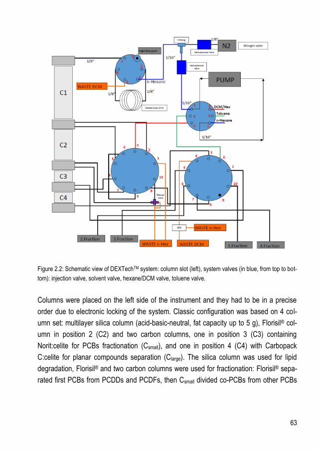
63
Figure 2.2: Schematic view of DEXTechTM system: column slot (left), system valves (in blue, from top to bot-
tom): injection valve, solvent valve, hexane/DCM valve, toluene valve.
Columns were placed on the left side of the instrument and they had to be in a precise
order due to electronic locking of the system. Classic configuration was based on 4 col-
umn set: multilayer silica column (acid-basic-neutral, fat capacity up to 5 g), Florisil® col-
umn in position 2 (C2) and two carbon columns, one in position 3 (C3) containing
Norit:celite for PCBs fractionation (Csmall), and one in position 4 (C4) with Carbopack
C:celite for planar compounds separation (Clarge). The silica column was used for lipid
degradation, Florisil® and two carbon columns were used for fractionation: Florisil® sepa-
rated first PCBs from PCDDs and PCDFs, then Csmall divided co-PCBs from other PCBs
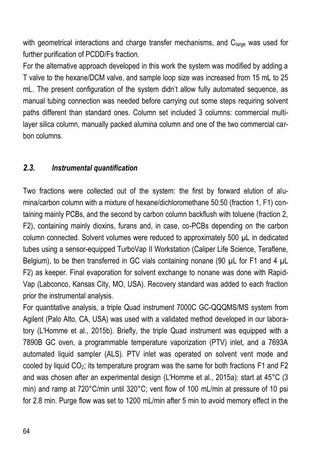
64
with geometrical interactions and charge transfer mechanisms, and Clarge was used for
further purification of PCDD/Fs fraction.
For the alternative approach developed in this work the system was modified by adding a
T valve to the hexane/DCM valve, and sample loop size was increased from 15 mL to 25
mL. The present configuration of the system didn’t allow fully automated sequence, as
manual tubing connection was needed before carrying out some steps requiring solvent
paths different than standard ones. Column set included 3 columns: commercial multi-
layer silica column, manually packed alumina column and one of the two commercial car-
bon columns.
2.3. Instrumental quantification
Two fractions were collected out of the system: the first by forward elution of alu-
mina/carbon column with a mixture of hexane/dichloromethane 50:50 (fraction 1, F1) con-
taining mainly PCBs, and the second by carbon column backflush with toluene (fraction 2,
F2), containing mainly dioxins, furans and, in case, co-PCBs depending on the carbon
column connected. Solvent volumes were reduced to approximately 500 µL in dedicated
tubes using a sensor-equipped TurboVap II Workstation (Caliper Life Science, Teraflene,
Belgium), to be then transferred in GC vials containing nonane (90 µL for F1 and 4 µL
F2) as keeper. Final evaporation for solvent exchange to nonane was done with Rapid-
Vap (Labconco, Kansas City, MO, USA). Recovery standard was added to each fraction
prior the instrumental analysis.
For quantitative analysis, a triple Quad instrument 7000C GC-QQQMS/MS system from
Agilent (Palo Alto, CA, USA) was used with a validated method developed in our labora-
tory (L'Homme et al., 2015b). Briefly, the triple Quad instrument was equipped with a
7890B GC oven, a programmable temperature vaporization (PTV) inlet, and a 7693A
automated liquid sampler (ALS). PTV inlet was operated on solvent vent mode and
cooled by liquid CO2; its temperature program was the same for both fractions F1 and F2
and was chosen after an experimental design (L'Homme et al., 2015a): start at 45°C (3
min) and ramp at 720°C/min until 320°C; vent flow of 100 mL/min at pressure of 10 psi
for 2.8 min. Purge flow was set to 1200 mL/min after 5 min to avoid memory effect in the

65
inlet. GC column was the classic DB-5ms 60 m x 250 µm x 0.25 µm (Agilent). Injection
volume was 2 µL for F1 and 5 µL for F2, and GC oven temperature program was differ-
ent for the two fractions as well. For F2 oven program started at 120°C (5 min), ramped
up at 25°C/min until 250°C (5 min), then 3°C/min until 285°C (15 min) for a total runtime
of 41.6 min. For F1 the program started the same, but temperature was set at 285°C for 0
min. The transfer line temperature was held at 280°C in both cases. On the MS side,
7000C electron ionization (EI) ion source was heated at 280°C and operated at 70 eV.
Quadrupoles were held at 150°C, nitrogen collision gas was flowing at 1.5 mL/min, and
helium quench gas at 2.25 mL/min. Quads resolution was set to unit mass, which by de-
fault corresponds to peak width of 0.7 Da at half height.
3. Results and discussion
3.1. Classic clean-up scheme
Classic clean-up method for DEXTexh system was based on 4 column set: multilayer sil-
ica- Florisil®-two carbon columns. Classic procedure followed the same well-proven prin-
ciple as the manual CVUA-MEL clean-up (Bernsmann T. et al., 2014).
Organic solvent from Soxhlet extraction or pure fat was dissolved in 2 mL toluene and 3
mL n-hexane, and manually injected with a syringe into the sample loop. The process
(Table 2.1) starts with a column conditioning step (from 1 to 3). Then sample is automati-
cally collected with hexane from the sample loop and loaded with pure hexane on C1 sil-
ica column for lipid oxidation (steps 4 and 5). After 4 minutes C1/C2/C3 are connected in
line and fraction 1 (F1) containing I-PCBs is collected after carbon column C3, while MO-
and co-PCBs are loaded on C3 (step 6). In step 7, Florisil® column C2 is backflushed with
hexane/DCM 50/50 mixture to transfer dioxins and furans from the top of the Florisil® to
the carbon column C4. Afterwards C3 is eluted with hexane/DCM (50/50) mixture to col-
lect fraction 2 (F2) of MO-PCBs (step 8). C3 is backflushed with toluene in step 9 to col-
lect co-PCBs (F3). Finally in step 10 carbon column C4 is backflushed with toluene to col-
lect fraction 4 (F4) containing planar PCDD/Fs. Solvent flow rate was always set at 7
mL/min, except in step 9 where it was 1 mL/min.
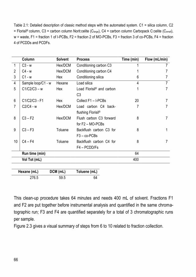
66
Table 2.1: Detailed description of classic method steps with the automated system. C1 = silica column, C2
= Florisil® column, C3 = carbon column Norit:celite (Clarge), C4 = carbon column Carbopack C:celite (Csmall),
w = waste, F1 = fraction 1 of I-PCBs, F2 = fraction 2 of MO-PCBs, F3 = fraction 3 of co-PCBs, F4 = fraction
4 of PCDDs and PCDFs.
Hexane (mL) DCM (mL) Toluene (mL)
276.5 59.5 64
This clean-up procedure takes 64 minutes and needs 400 mL of solvent. Fractions F1
and F2 are put together before instrumental analysis and quantified in the same chroma-
tographic run; F3 and F4 are quantified separately for a total of 3 chromatographic runs
per sample.
Figure 2.3 gives a visual summary of steps from 6 to 10 related to fraction collection.
Column Solvent Process Time (min) Flow (mL/min)
1 C3 - w Hex/DCM Conditioning carbon C3 1 7
2 C4 - w Hex/DCM Conditioning carbon C4 1 7
3 C1 - w Hex Conditioning silica 6 7
4 Sample loop/C1 - w Hexane Load silica 4 7
5 C1/C2/C3 – w Hex Load Florisil® and carbon
C3
1 7
6 C1/C2/C3 - F1 Hex Collect F1 – I-PCBs 20 7
7 C2/C4 - w Hex/DCM Load carbon C4 back-
flushing Florisil®
7 7
8 C3 – F2 Hex/DCM Flush carbon C3 forward
for F2 – MO-PCBs
8 7
9 C3 – F3 Toluene Backflush carbon C3 for
F3 – co-PCBs
8 1
10 C4 – F4 Toluene Backflush carbon C4 for
F4 – PCDD/Fs
8 7
Run time (min) 64
Vol Tot (mL) 400

67
Figure 2.3: Visual scheme of classic clean-up method with 4 column set: (left) steps from 6 to 7; (right)
steps from 8 to 10.
3.2. Alternative approach scheme
In the alternative approach proposed, 3 column set was used with the aim of solvent and
time reduction for high throughput protocols. In the classic method, Florisil® and two car-
bon columns are used for fractionation as Florisil® is not able to quantitatively separate or-
tho- and non-ortho PCBs, while complete separation is possible with alumina (Loos R.,
1997). In fact, in the developed method, alumina started the fractionation of planar and
non-planar compounds (including ortho- and non-ortho PCBs) which distribute at different
depth into the column. Then only one carbon column was needed to complete the frac-
tionation, based on geometrical and charge transfer interactions. Final fractionation de-
pends on the properties of the carbon sorbent (Concejero et al., 2001).
Main steps of the alternative method are described here (Table 2.2) and method devel-
opment is detailed in the following discussion. The method started with a short column

68
conditioning involving silica, alumina and carbon column in line, mainly to check for pos-
sible leaks or backpressure caused by manual column packing, before sample injection
into the system (step 1). Sample was injected in 25 mL sample loop and loaded with hex-
ane on C1 multilayer silica connected to manually packed basic alumina column (C2) in
position 2 (step 2). In this step C1 and C2 were connected to the waste turning the addi-
tional T valve and outlying a flow path not allowed in the classic system layout. The main
advantages of this configuration were that lipid degradation products formed on the silica
were purged out of the system, contrary to the classic method, and meanwhile analytes
were trapped on the basic alumina column. Manual connection of tubing was necessary
in step 3 to elute alumina column fraction towards carbon column in position 3 (Clarge or
Csmall) with hexane/DCM 50/50 mixture and collect fraction 1 (F1) containing PCBs. In the
meantime, planar compounds eluting from alumina were trapped on the top of carbon
column because of electronic and geometrical interactions, to be collected in fraction 2
(F2) by backflushing with toluene in step 4.
Table 2.2: Main steps of the alternative clean-up approaches using 3 column set: silica (C1) – alumina (C2)
- carbon (C3) column.
Column Solvent Process
1 C1/C2/C3 - w Hexane Conditioning system
2 Sample loop/C1/C2 - w Hexane Load silica and alumina, purge
3 C2/C3 – F1 Hexane/DCM Elute alumina, load carbon, collect F1
4 C3 – F4 Toluene Backflush carbon C3 for F2
The alternative method used only 3 columns instead of 4, and only 4 steps were needed
for complete sample clean-up. Final method performances and fractionation profile were
different based on carbon column used to complete fractionation, as described in the fol-
lowing discussion. Figure 2.4 gives a visual summary of the new method from step 2 to 4.

69
Figure 2.4: Alternative clean-up scheme with 3 column set and basic alumina. Two fractions were collected
and their composition varied with the carbon column used. A T valve was added to the central valve of the
system to allow purging after alumina column, which was not possible in the classic configuration of the
system.
This method was developed step by step optimizing solvent volume and time. Flow rate
was always hold at 7 mL/min in all the steps as in the classic method.

70
3.2.1. Conditioning step
The conditioning step was considerably shortened in comparison to the classic method,
because no difference in background levels was found when skipping this step. Just a
short preliminary silica-alumina and carbon column flushing in a row with hexane was
maintained to check for possible leaks or backpressure in the automated system. In some
cases in fact, the system recorder high backpressure and stopped automatically. Likely,
as the alumina column was manually packed, little experimental variation in sorbent
amount or filters placement into the column, led to solvent flow hindrance and resulting
backpressure. Conditioning step took 8 minutes, which corresponded to the sum of the
dead volumes of each column: 6 minutes for standard multilayer silica, 1 minute for alu-
mina and 1 minute for the carbon.
3.2.2. Silica column elution profile
Multilayer silica column elution profile was studied to assess the volume of hexane re-
quired to bring all the analytes out of the silica and to load them onto the alumina. Com-
mercial multilayer silica column with fat capacity up to 5 g were used. Its exact composi-
tion was unknown, but basically it contained layers of Na2SO4, 44% acidic, neutral and
basic silica.
For method development, samples consisted of 2 mL of hexane spiked with 13C labelled
IS of all the congeners and injected in the automated clean-up system with a glass sy-
ringe. Elution profiles were outlined collecting fractions every 5 minutes directly after the
silica column with hexane flowing at 7 mL/min. Each fraction was evaporated and spiked
with RS to assess the percentage of compounds eluting during time. Figure 2.5 showed
the elution profiles of I- and MO-PCBs, indicated as PCB fraction, and co-PCBs, PCCDs
and PCDFs, called dioxin fraction even if no fractionation occurred on the silica column.
This was due to our normal instrumental setup, detecting PCBs and dioxins separately.
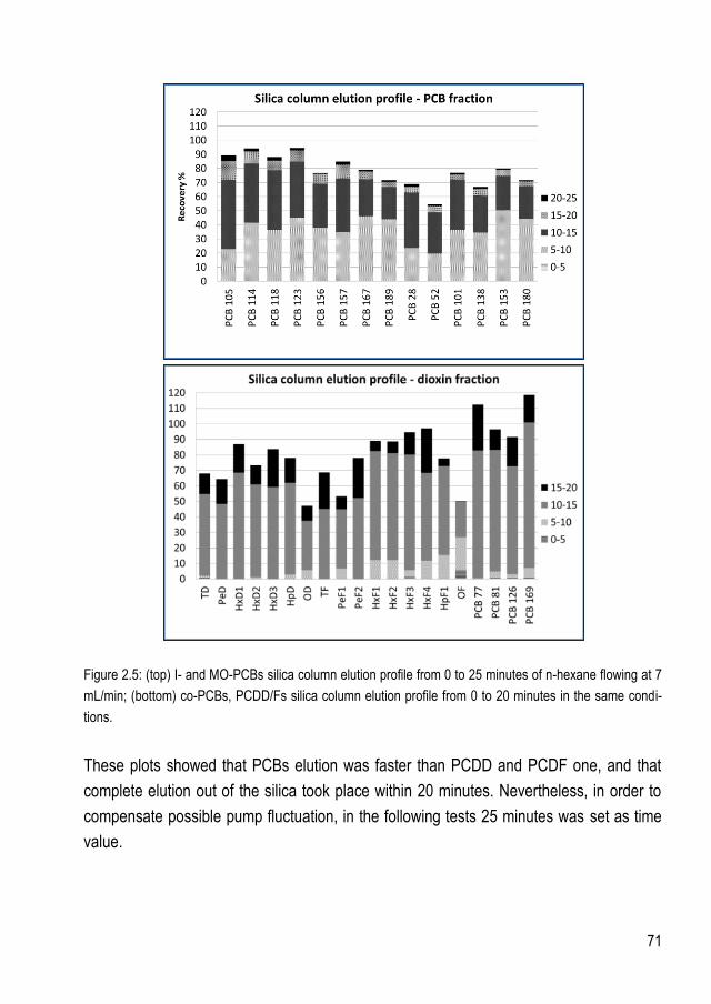
71
Figure 2.5: (top) I- and MO-PCBs silica column elution profile from 0 to 25 minutes of n-hexane flowing at 7
mL/min; (bottom) co-PCBs, PCDD/Fs silica column elution profile from 0 to 20 minutes in the same condi-
tions.
These plots showed that PCBs elution was faster than PCDD and PCDF one, and that
complete elution out of the silica took place within 20 minutes. Nevertheless, in order to
compensate possible pump fluctuation, in the following tests 25 minutes was set as time
value.

72
3.2.3. Alumina column
The alumina column was manually packed with commercial alumina. Both commercial
neutral and basic alumina were already activated at Brockmann grade I, with ~150 mesh
particle size and 58Å pore size. Normally, basic alumina has a pH of 9-10 and it is used to
separate basic and neutral compounds stable to alkali; neutral alumina has pH 6 – 8 and
is used for less polar compounds (1994). Basic and neutral alumina can be prepared in
various activity grades (I to V) based on the Brockmann scale:
Activity grade I II III IV V
Water added (wt %) 0 3 6 10 15
Grade I is prepared by heating alumina until complete water removal, typically overnight
at 400-450°C; the other grades are prepared by adding water to Grade I to deactivate it.
In this work, the alumina column needed for PCB and dioxin fractionation was manually
packed using the same scheme and the same components of the commercial Florisil®
column for the DEXTechTM system (Figure 2.6).
Figure 2.6: Packing scheme and components used in the commercial Florisil® column.
Alumina column size had to be the same as commercial Florisil® because of the elec-
tronic locking of the automated system based on fixed dimension. Such a column was

73
able to host 10-11 g of sorbent, and this represented a constraint for method develop-
ment, as well as the silica column size. Alumina sorbent, in fact, had to be active enough
to trap all the analytes, preventing their loss into the waste despite using an imposed lim-
ited amount of maximum 11 g, and despite 175 mL of hexane flowing at 7 mL/min. Figure
2.7 showed the experiment designed to assess the suitability of alumina material: 2 mL of
hexane spiked with labelled IS of all the congeners were injected in the system and
loaded/eluted with 175 mL of hexane on the silica column connected to manually packed
alumina column and to the waste. Afterwards alumina was eluted with hexane/DCM 50/50
mixture to calculate recovery rates, which had to be in the range 60-120 % as required by
EU Regulation. Two fractions were collected for each experiment: the waste and alumina
eluate, to check if interesting compounds were lost in the waste or were trapped on the
alumina column and then eluted with hexane/DCM 50/50 mixture. Only PCBs elution was
assessed, being the first eluting compounds, followed by dioxins and furans.
Figure 2.7: Flow scheme of the experiment designed to assess the suitability of alumina: the model sample
was injected and loaded on the silica column connected in line with the alumina column end ending into the
waste. Two fractions were collected and analysed to check the compound distribution: the waste and the
fraction eluting from alumina column

74
Preliminary tests using commercial Brockmann I neutral and basic alumina with no addi-
tional treatment showed immediately that for our purposes basic alumina was more effec-
tive than neutral, revealing that sorbent basicity played an important role in interaction
with compounds. For this reason successive testing was focused only on basic alumina.
Super-basic materials were prepared according to reported procedures (Ramos et al.,
1997, Xie et al., 2006) but these materials lead recovery rates lower than 60% estab-
lished by EU Regulation. Then thermal activation of alumina was assessed as a possible
way to enhance material basicity by water and CO2 removal from the active sites. Ther-
mal treatment suggested in EPA 1613 method was tried first: basic alumina was baked
for 30 hours at 600°C and cooled down to 130°C in desiccators before use. Material so
prepared showed higher recovery rates than before, but some compounds were still lost
in the waste in our experimental conditions (Figure 2.8).
Figure 2.8: Distribution of PCBs between waste and alumina column when using thermal treatment in EPA
1613, cooling down alumina at 130°C after 30 h backing at 600°C.
Even if not usable in the method development, this experiment was very important to re-
veal interaction mechanism between compounds and alumina sorbent. Results displayed
that, taking into account PCBs dipole moment (µ) calculated in a previous work with mo-
lecular modelling (Pirard et al., 2002), polar PCBs (µ > 1) were more retained on the sor-
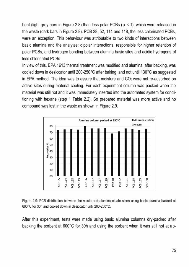
75
bent (light grey bars in Figure 2.8) than less polar PCBs (µ < 1), which were released in
the waste (dark bars in Figure 2.8). PCB 28, 52, 114 and 118, the less chlorinated PCBs,
were an exception. This behaviour was attributable to two kinds of interactions between
basic alumina and the analytes: dipolar interactions, responsible for higher retention of
polar PCBs, and hydrogen bonding between alumina basic sites and acidic hydrogens of
less chlorinated PCBs.
In view of this, EPA 1613 thermal treatment was modified and alumina, after backing, was
cooled down in desiccator until 200-250°C after baking, and not until 130°C as suggested
in EPA method. The idea was to assure that moisture and CO2 were not re-adsorbed on
active sites during material cooling. For each experiment column was packed when the
material was still hot and it was immediately inserted into the automated system for condi-
tioning with hexane (step 1 Table 2.2). So prepared material was more active and no
compound was lost in the waste as shown in Figure 2.9.
Figure 2.9: PCB distribution between the waste and alumina eluate when using basic alumina backed at
600°C for 30h and cooled down in desiccator until 200-250°C.
After this experiment, tests were made using basic alumina columns dry-packed after
backing the sorbent at 600°C for 30h and using the sorbent when it was still hot at ap-

76
proximately ~250°C. It is important to underline that even if alumina column was packed
with hot material, it was operating at room temperature during all sample clean-up steps.
3.2.4. Carbon column
The last step of method development was the connection of the carbon column in line
with the alumina for PCB and dioxin complete fractionation. Two carbon columns were
commercially available Clarge (Carbopack C:celite) and Csmall (Norit:celite) exhibiting differ-
ent fractionation properties (Concejero et al., 2001). In this set of experiments, 2 mL of
hexane spiked with labelled IS of all the congeners were injected in the system and
loaded on the alumina column with 175 mL of hexane. Alumina fraction was eluted with
hexane/DCM 50/50 mixture towards the carbon column and fractions were collected after
the carbon to assess its elution profile and recoveries.
3.2.4.1. Clarge - Carbopack C:celite elution profile
Clarge column, containing Carbopack C:celite mixture, whose position is the number 4 in
the classic system configuration, was placed in position 3 after the alumina column. A
dummy column was placed in position 4 to allow system locking. Fractionation profile of
Clarge flushing with hexane/DCM mixture was calculated to assess the volume needed to
elute all the compounds. The first fraction was collected after 5 minutes and then every
minute until 8 min in order to avoid oversplitting and to allow a better assessment of re-
quired volume (Figure 2.10).

77
Figure 2.10: Clarge column PCB elution profile. Carbon was eluted with hexane/DCM 50/50 mixture at 7
mL/min in forward direction.
I- and MO-PCBs elution time using Clarge was 6 minutes with hexane/DCM 50/50 mixture
flowing at 7 mL/min. With this column co-PCBs were collected together with other PCBs
in forward direction flush, despite their different planar structure. Whereas PCDDs and
PCDFs were still trapped on the top of the carbon column and were collected in backflush
with toluene for 8 minutes as in the classic method (Table 2.1). Recoveries were in the
range 60-120% for all congener in both fractions.
So, the clean-up method using silica-alumina-Carbopack C:celite columns lead to this
fractionation profile: all the PCBs, I-, MO- and co-PCBs were collected in fraction 1,
PCDDs and PCDFs were found in fraction 2. Method steps and performances are re-
ported in Table 2.3.
Re
cove
ry %

78
Table 2.3: “Alumina – Carbopack C” method steps and performances in terms of run time and total sample
volume.
Column Solvent Process Time
(min)
Flow
(mL/min)
1 C1/C2/C3 - w Hex Conditioning system 8 7
2 Sample loop/C1/C2 - w Hex Load silica and alumina, purge 25 7
3 C2/C3 – F1 Hex/DCM Elute alumina, load carbon, col-
lect F1
6 7
4 C3 – F2 Toluene Backflush carbon C3 for F2 8 7
Run time (min) 47 -26.6%
Vol Tot (mL) 329 -17.8%
If compared with classic method, “alumina-Carbopack C method” allowed about 18% of
solvent saving and 27% of time saving (See Table 2.5 for comparison)
3.2.4.2. Csmall – Norit:celite elution profile
Csmall carbon column, containing Norit:celite mixture is usually found in position 3 in clas-
sic system configuration. In this work, Csmall was still in position 3, but a dummy column
was placed in position 4, just for electronic system locking. 2 mL of hexane spiked with
labelled IS of all the congeners were injected in the system, loaded on the silica and alu-
mina column and finally eluted from the alumina with hexane/DCM 50/50 mixture towards
the carbon column. Fractions were collected every 2 minutes for 8 minutes after the car-
bon and injected on the Triple Quad for recovery and fractionation profile assessment
(Figure 2.11)
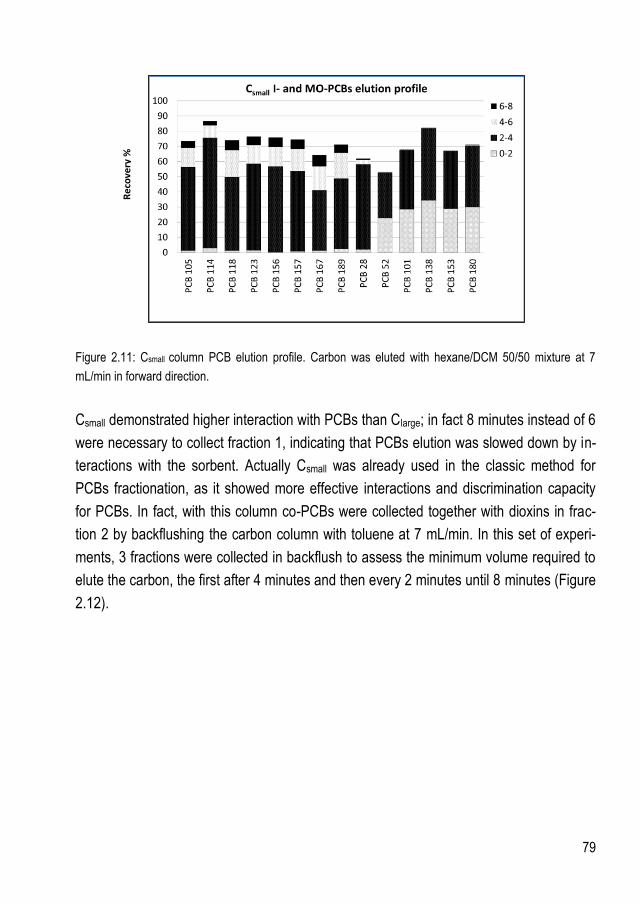
79
Figure 2.11: Csmall column PCB elution profile. Carbon was eluted with hexane/DCM 50/50 mixture at 7
mL/min in forward direction.
Csmall demonstrated higher interaction with PCBs than Clarge; in fact 8 minutes instead of 6
were necessary to collect fraction 1, indicating that PCBs elution was slowed down by in-
teractions with the sorbent. Actually Csmall was already used in the classic method for
PCBs fractionation, as it showed more effective interactions and discrimination capacity
for PCBs. In fact, with this column co-PCBs were collected together with dioxins in frac-
tion 2 by backflushing the carbon column with toluene at 7 mL/min. In this set of experi-
ments, 3 fractions were collected in backflush to assess the minimum volume required to
elute the carbon, the first after 4 minutes and then every 2 minutes until 8 minutes (Figure
2.12).
Re
cove
ry %
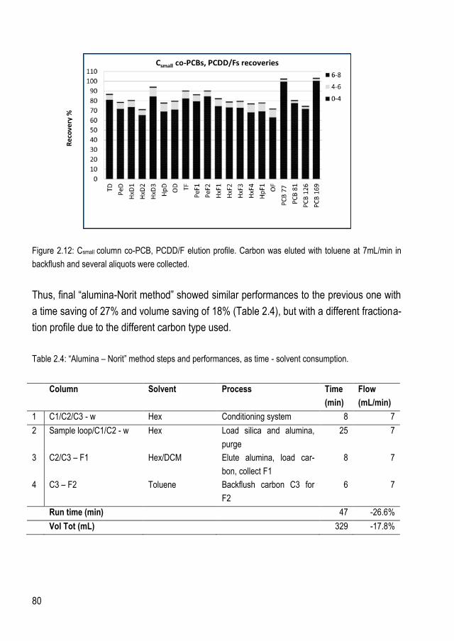
80
Figure 2.12: Csmall column co-PCB, PCDD/F elution profile. Carbon was eluted with toluene at 7mL/min in
backflush and several aliquots were collected.
Thus, final “alumina-Norit method” showed similar performances to the previous one with
a time saving of 27% and volume saving of 18% (Table 2.4), but with a different fractiona-
tion profile due to the different carbon type used.
Table 2.4: “Alumina – Norit” method steps and performances, as time - solvent consumption.
Column Solvent Process Time
(min)
Flow
(mL/min)
1 C1/C2/C3 - w Hex Conditioning system 8 7
2 Sample loop/C1/C2 - w Hex Load silica and alumina,
purge
25 7
3 C2/C3 – F1 Hex/DCM Elute alumina, load car-
bon, collect F1
8 7
4 C3 – F2 Toluene Backflush carbon C3 for
F2
6 7
Run time (min) 47 -26.6%
Vol Tot (mL) 329 -17.8%
Re
cove
ry %
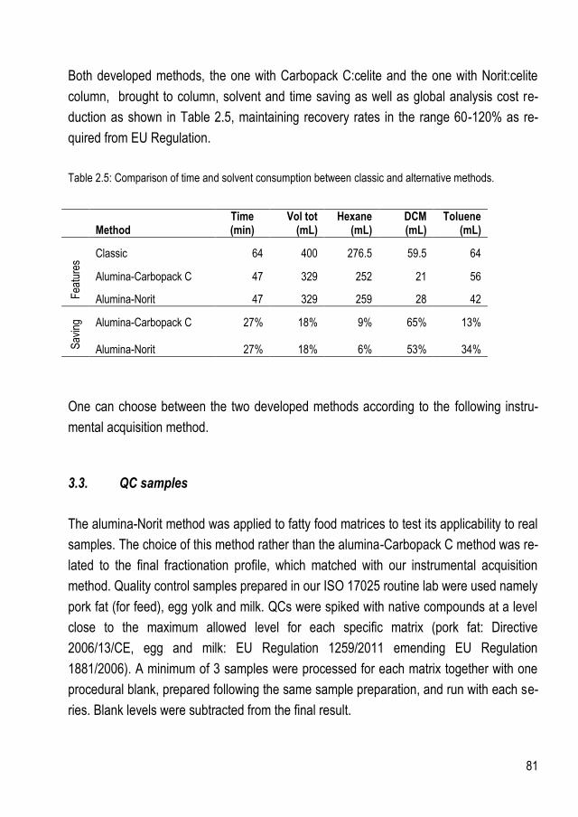
81
Both developed methods, the one with Carbopack C:celite and the one with Norit:celite
column, brought to column, solvent and time saving as well as global analysis cost re-
duction as shown in Table 2.5, maintaining recovery rates in the range 60-120% as re-
quired from EU Regulation.
Table 2.5: Comparison of time and solvent consumption between classic and alternative methods.
Method
Time (min)
Vol tot (mL)
Hexane (mL)
DCM (mL)
Toluene (mL)
Fea
ture
s
Classic 64 400 276.5 59.5 64
Alumina-Carbopack C 47 329 252 21 56
Alumina-Norit 47 329 259 28 42
Sav
ing
Alumina-Carbopack C 27% 18% 9% 65% 13%
Alumina-Norit 27% 18% 6% 53% 34%
One can choose between the two developed methods according to the following instru-
mental acquisition method.
3.3. QC samples
The alumina-Norit method was applied to fatty food matrices to test its applicability to real
samples. The choice of this method rather than the alumina-Carbopack C method was re-
lated to the final fractionation profile, which matched with our instrumental acquisition
method. Quality control samples prepared in our ISO 17025 routine lab were used namely
pork fat (for feed), egg yolk and milk. QCs were spiked with native compounds at a level
close to the maximum allowed level for each specific matrix (pork fat: Directive
2006/13/CE, egg and milk: EU Regulation 1259/2011 emending EU Regulation
1881/2006). A minimum of 3 samples were processed for each matrix together with one
procedural blank, prepared following the same sample preparation, and run with each se-
ries. Blank levels were subtracted from the final result.
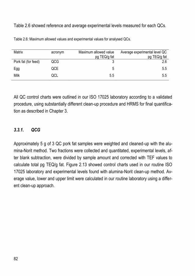
82
Table 2.6 showed reference and average experimental levels measured for each QCs.
Table 2.6: Maximum allowed values and experimental values for analysed QCs.
Matrix acronym Maximum allowed value pg TEQ/g fat
Average experimental level QC pg TEQ/g fat
Pork fat (for feed) QCG 3 2.6
Egg QCE 5 5.5
Milk QCL 5.5 5.5
All QC control charts were outlined in our ISO 17025 laboratory according to a validated
procedure, using substantially different clean-up procedure and HRMS for final quantifica-
tion as described in Chapter 3.
3.3.1. QCG
Approximately 5 g of 3 QC pork fat samples were weighted and cleaned-up with the alu-
mina-Norit method. Two fractions were collected and quantitated, experimental levels, af-
ter blank subtraction, were divided by sample amount and corrected with TEF values to
calculate total pg TEQ/g fat. Figure 2.13 showed control charts used in our routine ISO
17025 laboratory and experimental levels found with alumina-Norit clean-up method. Av-
erage value, lower and upper limit were calculated in our routine laboratory using a differ-
ent clean-up approach.
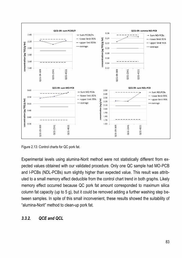
83
Figure 2.13: Control charts for QC pork fat.
Experimental levels using alumina-Norit method were not statistically different from ex-
pected values obtained with our validated procedure. Only one QC sample had MO-PCB
and I-PCBs (NDL-PCBs) sum slightly higher than expected value. This result was attrib-
uted to a small memory effect deducible from the control chart trend in both graphs. Likely
memory effect occurred because QC pork fat amount corresponded to maximum silica
column fat capacity (up to 5 g), but it could be removed adding a further washing step be-
tween samples. In spite of this small inconvenient, these results showed the suitability of
“alumina-Norit” method to clean-up pork fat.
3.3.2. QCE and QCL

84
Freeze dried QC egg yolks were processed as described in the experimental section. Ex-
tracted fat was spiked with IS solutions and diluted with 5 mL of hexane to be injected in
the automated system and cleaned-up accordingly to “alumina-Norit” method. Figure 2.14
(top) showed the comparison between reference values and average experimental values
of three QC samples, which were not statistically different and demonstrated the applica-
bility of “alumina-Norit” method to egg yolks. The same approach was applied to milk QCs
and similar results were obtained (Figure 2.14, bottom).
Figure 2.14: Reference and experimental values for egg yolk (top) and milk (bottom) quality control sam-
ples. PCDD/Fs, MO- and co-PCBs are expressed in pg TEQ/g fat; I-PCBs are in ng/g as they don’t have a
TEF assigned.

85
In both cases, some egg yolk and milk samples were not valid due to interferences in in-
strumental quantification of hexa- and hepta-dioxins and furans, which heavily contribute
to final TEQ calculation. For these samples, fraction 2, the most critic one, looked yellow-
ish even after clean-up, indicating the presence of undesirable compounds, which was
probably related to manual packing of the alumina column because it occurred random-
lµy. Maybe high temperature packing had a negative effect on column components not
designed for this scope. The clean-up method seemed to be not robust but nevertheless
reliable because it led to accurate TEQ calculation when no interferences were released.
4. Conclusions
Alternative clean-up approaches were developed and implemented in an already auto-
mated clean-up system. This work was aimed to reduce global cost of the analysis in
comparison with the currently used method. New approaches were based on 3 column
set instead of 4, namely multilayer silica, basic alumina and one carbon column. Multi-
layer silica and two carbon columns were commercially available, while alumina column
was manually packed after proper thermal treatment based on a modified EPA 1613 pro-
cedure. The two approaches arose from the availability of two different carbon columns
leading to different final fractionation profiles: with Carbopack C:celite column, I-, MO- and
co-PCBs were collected in fraction 1, and PCDD/Fs were found infraction 2, with
Norit:celite column, co-PCBs were found in fraction 2 together with dioxins. It is thus pos-
sible to choose the appropriate protocol based on the consecutive instrumental analysis.
The new developed approaches allowed time and solvent saving, respectively 27% and
18%, as well as global cost reduction, giving recoveries in the range 60-120% as required
by EU Regulation.
The “Alumina-Norit” method was applied to QC samples of pork fat, egg yolk and milk to
assess its performances on real fatty matrices and results showed that the clean-up
method was accurate, despite some issues related to manual packing. A full validation
was not carried out because of the high variability of the manual packing and because it
was out of the scope to validate a non-fully automated method using manually packed
column. These preliminary results, however, could be a starting point for full validation of
a clean-up method using DEXTechTM system (equipped with a T valve that switches

86
automatically) and alumina columns produced industrially. Implementing a fully auto-
mated alumina column method would be interesting due to global cost reduction of this
method.
87
Bibliography
1994. EPA Mthod 1613 - Tetra- through Octa-Chlorinated Dioxins and Furans by Isotope Dlution HRGC/HRMS.
2014a. COMMISSION REGULATION (EU) No 589/2014 of 2 June 2014 laying down methods of sampling and analysis for the control of levels of dioxins, dioxin-like PCBs and non-dioxin-like PCBs in certain foodstuffs and repealing Regulation (EU) No 252/2012.
2014b. COMMISSION REGULATION (EU) No 709/2014 of 20 June 2014 amending Regulation (EC) No 152/2009 as regards the determination of the levls of dioxins and polychlorinated biphenyls
ARIES, E., ANDERSON, D. R., ORDSMITH, N., HALL, K. & FISHER, R. 2004. Development and validation of a method for analysis of " dioxin-like" PCBs in environmental samples from the steel industry. Chemosphere, 54, 23-31.
BERNSMANN T., ALBRECHT M. & FÜRST P. 2014. FAST SAMPLE PREPARATION FOR ROUTINE DETERMINATION OF PCDD/F, PCB AND PBDE IN FOOD AND FEED. Organohalogen Compounds, 76, 1281-1284.
CONCEJERO, M., RAMOS, L., JIMÉNEZ, B., GÓMARA, B., ABAD, E., RIVERA, J. & GONZÁLEZ, M. J. 2001. Suitability of several carbon sorbents for the fractionation of various sub-groups of toxic polychlorinated biphenyls, polychlorinated dibenzo-p-dioxins and polychlorinated dibenzofurans. Journal of Chromatography A, 917, 227-237.
FÜRST, P. 2006. Dioxins, polychlorinated biphenyls and other organohalogen compounds in human milk. Molecular Nutrition and Food Research, 50, 922-933.
L'HOMME, B., CALAPRICE, C., CALVANO, C. D., ZAMBONIN, C., LEARDI, R. & FOCANT, J. F. 2015a. Ultra-trace measurement of Dechloranes to investigate food as a route of human exposure. Chemosphere, 139, 525-533.
L'HOMME, B., SCHOLL, G., EPPE, G. & FOCANT, J. F. 2015b. Validation of a gas chromatography-triple quadrupole mass spectrometry method for confirmatory analysis of dioxins and dioxin-like polychlorobiphenyls in feed following new EU Regulation 709/2014. Journal of Chromatography A, 1376, 149-158.
LOOS R., V. S., NIESSNER R. 1997. Group separation of ortho-PCBs, coplanar non-ortho PCbs and PCDD/PCDFs using alumina column as an one-step clean-up procedure. Fresenius J Anal Chem 357, 7.
PIRARD, C., FOCANT, J. F. & DE PAUW, E. 2002. An improved clean-up strategy for simultaneous analysis of polychlorinated dibenzo-p-dioxins (PCDD), polychlorinated dibenzofurans (PCDF), and polychlorinated biphenyls (PCB) in fatty food samples. Fresenius' Journal of Analytical Chemistry, 372, 373-381.

88
RAMOS, L., HERNANDEZ, L. M. & GONZALEZ, M. J. 1997. Elution pattern of planar chlorinated biphenyls and 2,3,7,8-polychlorinated dibenzo-p-dioxins/dibenzofurans on chromatographic adsorbents and factors affecting the mechanism of retention. Possibilities of selective separation of both families. Journal of Chromatography A, 759, 127-137.
SAFE, S. 1990. Polychlorinated biphenyls (PCBs), dibenzo-p-dioxins (PCDDs), dibenzofurans (PCDFs), and related compounds: Environmental and mechanistic considerations which support the development of toxic equivalency factors (TEFs). Critical Reviews in Toxicology, 21, 51-88.
XIE, W., PENG, H. & CHEN, L. 2006. Transesterification of soybean oil catalyzed by potassium loaded on alumina as a solid-base catalyst. Applied Catalysis A: General, 300, 67-74.

89
CHAPTER III
Revisiting an existing dioxin/PCB clean-up and fractionation procedure to re-
duce solvent and time consumption
1. Introduction
Alternative automated clean-up approaches using PowerPrepTM system from Fluid Man-
agement Systems (FMS Inc., Waltham, MA, USA) have been implemented and tested on
food and feed matrices for the low level analysis of polychlorinated dibenzo-p-dioxins,
polychlorinated dibenzofurans, dioxin like and non-dioxin like regulated PCBs. This work
was carried out in the perspective of a cheaper and more sustainable procedure, as well
as faster a high throughput method for food safety (Abad et al., 2000, Fujita et al., 2009).
In the first part of the work our validated procedure employing PowerPrepTM was opti-
mized for low fat matrices; in the second part, a fully automated approach was tested and
compared to our routine procedure for fat content up to 4 g.
2. Materials and method
2.1. Chemicals and consumables
Solvents (hexane, dichloromethane, toluene, methanol) were Picograde® reagents (LGC
Promochem, Wesel, Germany). All solvent batches were tested for the investigated ana-
lytes contamination before use. Nonane puriss analytical-reagent grade standard for GC
was purchased from Fluka (Steinheim, Germany). Disposable PTFE columns for the
automated clean-up were obtained from Fluid Management Systems (FMS Inc., Waltham,
MA, USA).
Chromatographic pure grade helium gas, 99.9999% alphagaz 2 was purchased from Air
Liquide (Paris, France). Technical N27 grade liquid CO2 was used for PTV cooling (Air
Liquide, Paris, France). Disposable PTFE columns for the automated clean-up were ob-

90
tained from Fluid Management Systems (FMS Inc., Waltham, MA, USA). Reagent stan-
dards for native and 13C labelled PCDD/Fs and regulated PCBs, as well as calibration
curve solutions and recovery standards were the same described in Chapter II. Again,
analytes were quantitated by adding isotope dilution and 13C labelled IS solution prior
clean-up procedure (20 µL of internal standard mixture ST-ROU (13C-labelled PCDDs,
PCDFs, co-PCBs and MO-PCB) and 10 µL 13C I-PCBs solution). The recovery standard
was added to injection vial preceding the instrumental analysis for each fraction.
2.2. Sample preparation
For method development, only standard solutions were tested to assess recovery rates.
10 mL of hexane were spiked with IS solution and cleaned-up to check final recovery
rates. Thereafter, QC pork fat and sunflower oil were processed. None of these two ma-
trices required fat extraction as they were already pure fat. The QC was prepared in our
routine laboratory and spiked at the maximum allowed level (EU Directive 2006/13/CE),
sunflower oil was a food sample sent to our routine laboratory for regular analysis and its
levels were unknown. An aliquot of 4 g of each sample was weighted, spiked with labelled
IS solution and diluted in 60 mL of hexane to decrease viscosity and to disperse the fat.
The procedural blank, composed of 10 mL of hexane for both the fatty matrices, was
processed following exactly the same procedure as the samples. Samples were auto-
matically aspired and loaded on the PowerPrepTM system equipped with disposable PTFE
columns. In this work, different column sets and instrumental setups on PowerPrepTM sys-
tem were tested.
First setup was the standard one based on multilayer ABN silica (4 g acid, 2 g basic, 1.5
neutral), basic alumina (11 g), and carbon (0.34 g AX21) column, suitable for low fat con-
tent matrices (<1 g fat). A second setup using 4 column set, with higher fat capacity, was
proposed as follows: high capacity (HC) acidic silica column (45 g acidic silica 44%), mul-
tilayer mini silica column (2 g acid, 1 g basic, 0.5 g neutral), mini alumina column (6 g ba-
sic) and carbon column (0.34 g AX21) were used for fat amount up to 4 g. Mini silica and
alumina together with standard carbon column are usually referred to as FMS Mini Dioxin
prep kit. QC pork fat for feed and commercial sunflower oil were cleaned up with this in-
strumental setup to test its performances

91
As the carbon column didn’t change, the fractionation profile was the same in all the
cases and the two fractions were collected out of the automated system: fraction 1 (F1)
containing I- and MO-PCBs, and fraction 2 (F2) containing co-PCBs and PCDD/Fs. Frac-
tion solvents were evaporated to approximately 500 µL in dedicated tubes using a sen-
sor-equipped TurboVap II Workstation (Caliper Life Science, Teraflene, Belgium) and
then transferred in GC vials containing nonane (90 µL for F1 and 4 µL F2) as keeper.
The final evaporation for complete solvent exchange to nonane was done with RapidVap
(Labconco, Kansas City, MO, USA). Recovery standard was added to each fraction prior
the instrumental analysis.
2.2.1. PowerPrepTM automated system for sample clean-up
PowerPrepTM accurate description is out of the scope of this dissertation and is reported
elsewhere (Focant et al., 2001, Focant et al., 2006) but some aspects are worth to be
highlighted for the following discussion. The sample can be automatically loaded into the
system thanks to an aspiration valve (Figure 3.1, left). PowerPrepTM is designed to host
disposable PTFE columns after adding Teflon screw fittings, giving the possibility of ac-
commodating columns with variable size. Column set can be constituted by 3 or 4 col-
umns as shown later in the discussion. Column connection (Figure 3.1, right) is very flexi-
ble and customizable because of several 2 ways valves connected to each column; car-
bon column in particular is connected to double 2 way valves to allow backflush; 6 way
valves are used for solvent introduction and final collection. Such valve system allows
several flow schemes, column connection and disconnection via simple instrument soft-
ware. This design gives very flexible and customizable machine for several uses.
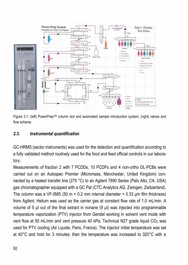
92
Figure 3.1: (left) PowerPrepTM column slot and automated sample introduction system; (right) valves and
flow scheme.
2.3. Instrumental quantification
GC-HRMS (sector instruments) was used for the detection and quantification according to
a fully validated method routinely used for the food and feed official controls in our labora-
tory.
Measurements of fraction 2 with 7 PCDDs, 10 PCDFs and 4 non-ortho DL-PCBs were
carried out on an Autospec Premier (Micromass, Manchester, United Kingdom) con-
nected by a heated transfer line (275 °C) to an Agilent 7890 Series (Palo Alto, CA, USA)
gas chromatographer equipped with a GC Pal (CTC Analytics AG, Zwingen, Zwitzerland).
The column was a VF-5MS (50 m × 0.2 mm internal diameter × 0.33 μm film thickness)
from Agilent. Helium was used as the carrier gas at constant flow rate of 1.0 mL/min. A
volume of 5 μl out of the final extract in nonane (9 μl) was injected into programmable
temperature vaporization (PTV) injector from Gerstel working in solvent vent mode with
vent flow at 50 mL/min and vent pressure 40 kPa. Technical N27 grade liquid CO2 was
used for PTV cooling (Air Lquide, Paris, France). The injector initial temperature was set
at 40°C and hold for 3 minutes; then the temperature was increased to 320°C with a

93
720°C/min ramp. This temperature was hold for 4 minutes before a second increase to
330°C, and kept until the end of the GC analysis. The oven temperature was maintained
at 60 °C for 5 min, ramped at 70 °C/min to 200 °C, ramped at 3.2 °C/min to 235 °C for
1.5 min, ramped at 3.2 °C/min to 270 °C for 10 min, and finally ramped at 15 °C/min to
310 °C for 13 min. The total separation time was 55 min. The HRMS instrument was op-
erated in selected ion monitoring (SIM) mode with mass resolution of at least 10,000 at a
10 % valley. The specificity was insured by monitoring the signal of two ions and compar-
ing their ion ratio to the theoretical chlorine isotope ratio.
Measurements of the 8 WHO mono-ortho PCBs and 6 I-PCBs were carried out on a
MAT95 (Thermo Fisher Scientific, Bremen, Germany) connected by a heated transfer line
(275 °C) to an Agilent 6890 Series gas chromatographer equipped with a A200S auto-
sampler. The column was an HT-8 (25 m × 0.22 mm ID × 0.25 μm film thickness) (SGE,
Villebon, France). Helium was used as the carrier gas at constant flow rate of 0.8 mL/min.
A volume of 2 μl from the final extract in nonane (100 μl) was injected into a split/splitless
injector held at 275 °C in splitless mode. A focus liner with glass wool form Agilent was
used for injection. The oven temperature was maintained at 140 °C for 2 min, ramped at
15.0 °C/min to 220 °C held for 7.5 min, ramped at 6.0 °C/min to 250 °C, ramped at 2.0
°C/min to 265 °C, and finally ramped at 28 °C/min to 320 °C. The total separation time
was 30 min. The HRMS instrument was operated in selected ion monitoring (SIM) mode
with a static resolving power of 10,000. Two ions were monitored for both native and la-
belled compounds for isotope ratio check.
More details on instrumental quantification are reported in a previous work (Focant et al.,
2001).
3. Results and discussion
3.1. Classic sample clean-up in our laboratory
In our laboratory, sample clean-up is based on two main steps: manually packed acidic
silica column followed by automated clean-up with PowerPrepTM using a 3 column set,
namely standard multilayer acidic-basic-neutral (ABN) silica column, basic alumina and

94
carbon column (AX-21) (Focant et al., 2004, Pirard et al., 2002, Focant and De Pauw,
2002). This approach has a fat capacity of up to 7 g and is outlined to have preliminary
lipid digestion which intensely reduces fat content up to maximum 1 g for all the matrices,
followed by automated clean-up which is the same for any matrix. This procedure is vali-
dated, robust, and represents a standardized approach for a great variety of food and
feed matrices.
3.1.1. Manual step
In our laboratory, preliminary lipid digestion is done with disposable glass column manu-
ally packed with acidic silica as follows (Figure 3.2): from the bottom, glass wool, 5 g
Na2SO4, 5 g neutral silica, 20 g 44% acidic silica, 20 g 22% acidic silica. Column is first
conditioned with 150 ml of hexane, and then sample is loaded and eluted with 150 mL of
hexane. Eluted solvent is evaporated to approximately 10 mL before being introduced in
the automated system. This manual step consumes 300 mL of hexane and takes from 30
to 45 minutes depending on fat nature.
Figure 3.2: Manually packed acidic silica column for lipid digestion
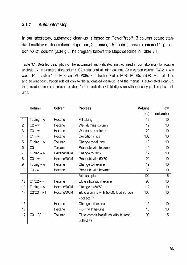
95
3.1.2. Automated step
In our laboratory, automated clean-up is based on PowerPrepTM 3 column setup: stan-
dard multilayer silica column (4 g acidic, 2 g basic, 1.5 neutral), basic alumina (11 g), car-
bon AX-21 column (0.34 g). The program follows the steps describe in Table 3.1.
Table 3.1: Detailed description of the automated and validated method used in our laboratory for routine
analysis, C1 = standard silica column, C2 = standard alumina column, C3 = carbon column (AX-21), w =
waste, F1 = fraction 1 of I-PCBs and MO-PCBs, F2 = fraction 2 of co-PCBs, PCDDs and PCDFs. Total time
and solvent consumption related only to the automated clean-up, and the manual + automated clean-up,
that included time and solvent required for the preliminary lipid digestion with manually packed silica col-
umn.
Column Solvent Process Volume
(mL)
Flow
(mL/min)
1 Tubing – w Hexane Fill tubing 15 10
2 C2 – w Hexane Wet alumina column 12 10
3 C3 – w Hexane Wet carbon column 20 10
4 C1 – w Hexane Condition silica 100 10
5 Tubing – w Toluene Change to toluene 12 10
6 C3 Toluene Pre-elute with toluene 40 10
7 Tubing – w Hexane/DCM Change to 50/50 12 10
8 C3 – w Hexane/DCM Pre-elute with 50/50 20 10
9 Tubing – w Hexane Change to hexane 12 10
10 C3 - w Hexane Pre-elute with hexane 30 10
11 Add sample 100 5
12 C1/C2 – w Hexane Elute silica with hexane 90 10
13 Tubing – w Hexane/DCM Change to 50/50 12 10
14 C2/C3 – F1 Hexane/DCM Elute alumina with 50/50, load carbon
- collect F1
100 10
15 Hexane Change to hexane 12 10
16 Hexane Flush with hexane 10 10
17 C3 – F2 Toluene Elute carbon backflush with toluene -
collect F2
90 5
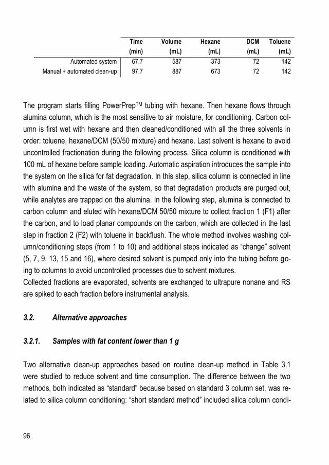
96
The program starts filling PowerPrepTM tubing with hexane. Then hexane flows through
alumina column, which is the most sensitive to air moisture, for conditioning. Carbon col-
umn is first wet with hexane and then cleaned/conditioned with all the three solvents in
order: toluene, hexane/DCM (50/50 mixture) and hexane. Last solvent is hexane to avoid
uncontrolled fractionation during the following process. Silica column is conditioned with
100 mL of hexane before sample loading. Automatic aspiration introduces the sample into
the system on the silica for fat degradation. In this step, silica column is connected in line
with alumina and the waste of the system, so that degradation products are purged out,
while analytes are trapped on the alumina. In the following step, alumina is connected to
carbon column and eluted with hexane/DCM 50/50 mixture to collect fraction 1 (F1) after
the carbon, and to load planar compounds on the carbon, which are collected in the last
step in fraction 2 (F2) with toluene in backflush. The whole method involves washing col-
umn/conditioning steps (from 1 to 10) and additional steps indicated as “change” solvent
(5, 7, 9, 13, 15 and 16), where desired solvent is pumped only into the tubing before go-
ing to columns to avoid uncontrolled processes due to solvent mixtures.
Collected fractions are evaporated, solvents are exchanged to ultrapure nonane and RS
are spiked to each fraction before instrumental analysis.
3.2. Alternative approaches
3.2.1. Samples with fat content lower than 1 g
Two alternative clean-up approaches based on routine clean-up method in Table 3.1
were studied to reduce solvent and time consumption. The difference between the two
methods, both indicated as “standard” because based on standard 3 column set, was re-
lated to silica column conditioning: “short standard method” included silica column condi-
Time
(min)
Volume
(mL)
Hexane
(mL)
DCM
(mL)
Toluene
(mL)
Automated system 67.7 587 373 72 142
Manual + automated clean-up 97.7 887 673 72 142

97
tioning, which was shortened in “fast standard method”. Both approaches were suitable
for low fat content matrices up to 1 g fat.
3.2.1.1. Short standard method
For method development, model samples consisting of 10 mL of hexane mimicking our
extracts were spiked with IS solution. Clean-up solvent volumes were optimized step by
step, measuring column and system dead volumes; silica, alumina and carbon column
elution profiles were outlined to insure the use of the minimum solvent amount. Detailed
description of method steps was reported in Table 3.2.
Table 3.2: “Short” and “fast” standard methods based on standard method in Table 3.1. Short method still
had silica column conditioning, which was removed in the fast method (see step 4).
New approaches started with filling the tubing to eliminate air from the system. 15 mL
were required as in the reference method, and this amount give and idea of the dead vol-
ume of the system. Thereafter, short wetting/conditioning step was carried out mainly to
check for possible leaks before sample introduction into the system. A minimum solvent
amount was used after dead volumes assessment.
SHORT FAST
Column Solvent Process Volume
(mL)
Volume
(mL)
Flow
(mL/min)
1 Tubing - w Hexane Fill tubing 15 15 10
2 C2 – w Hexane Wet alumina 12 12 10
3 C3 – w Hexane Wet carbon 6 6 10
4 C1 - w Hexane Condition/wet silica 100 12 10
5 Add sample 100 100 5
6 C1/C2 - w Hexane Elute silica with hexane 70 70 10
7 C2/C3 – F1 Hexane/DCM Elute alumina with 50/50,
collect F1 – load carbon
100 100 10
8 C3 – F2 Toluene Elute carbon backflush
with toluene - collect F2
90 90 5

98
“Short standard method”, as well as “fast standard method”, was based on classic
method, skipping less relevant steps. “Wash carbon column” steps (from 5 to 10 in the
reference method) were eliminated because commercial columns are produced in clean
rooms and sealed under vacuum to prevent any adsorption. Silica column elution volume
was set at 70 mL instead of 100 mL as a consequence of elution profile studies. Alumina
and carbon column elution volumes stayed the same as the reference after confirmation
of elution profiles. “Change solvent” steps in the reference method (5, 7, 9, 13, 15) were
removed because solvent exchange can take place directly onto the column with no effect
on fractionation. With the same logic, step 16 in the reference method was deleted be-
cause clean tubing from hexane/DCM 50/50 mixture before flushing toluene into the car-
bon column was not necessary. All the following discussion implies that preliminary steps
from 1 to 4 of short method have been carried out at the beginning of the run. Fast
method was developed later shortening only step 4 from 100 to 12 mL and calculating re-
coveries.
From step 1 to 4, silica and alumina column dead volumes were measured as the time
required for hexane at 10 mL/min passing through the column and it was found equal to
12 mL for both. Dead volume including tubing, namely the volume required for hexane at
10 mL/min to reach the waste after passing through the column, was 20 mL for both. Car-
bon column dead volume was 6 mL as this column was considerably smaller in size. Sil-
ica column conditioning in the “short standard method” was maintained the same as the
reference method (Table 3.1, step 4). This step was shortened in the “fast” method and
final performances were compared to assess if column conditioning could be skipped or
not.
After column wetting and conditioning, the sample was automatically aspired and loaded
on the silica (step 5). Silica column elution profile (Figure 3.3) was calculated to assess
the minimum solvent amount required for the complete elution of the column. Aliquots
were collected directly after the silica column every minute for 7 minutes for PCB fraction
(I- and MO-PCBs, F1), and every 2 minutes for 8 minutes for dioxin fraction (co-PCBs,
PCDD/Fs, F2), as dioxins are the last eluting compounds. Fraction profiles are shown
separately even if no fractionation occurred after the silica because of our instrumental
setup.
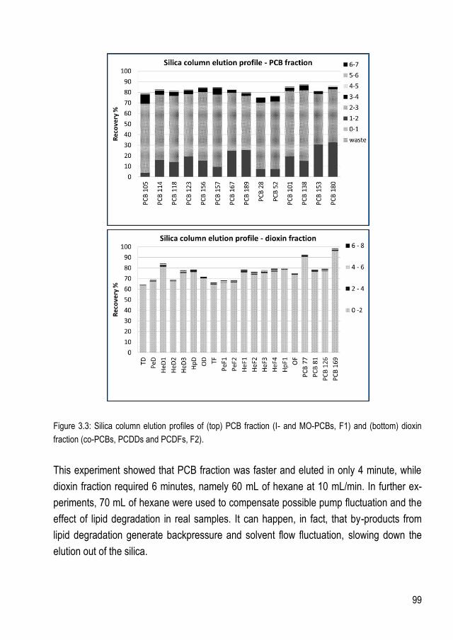
99
Figure 3.3: Silica column elution profiles of (top) PCB fraction (I- and MO-PCBs, F1) and (bottom) dioxin
fraction (co-PCBs, PCDDs and PCDFs, F2).
This experiment showed that PCB fraction was faster and eluted in only 4 minute, while
dioxin fraction required 6 minutes, namely 60 mL of hexane at 10 mL/min. In further ex-
periments, 70 mL of hexane were used to compensate possible pump fluctuation and the
effect of lipid degradation in real samples. It can happen, in fact, that by-products from
lipid degradation generate backpressure and solvent flow fluctuation, slowing down the
elution out of the silica.
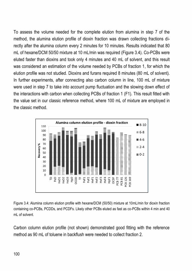
100
To assess the volume needed for the complete elution from alumina in step 7 of the
method, the alumina elution profile of dioxin fraction was drawn collecting fractions di-
rectly after the alumina column every 2 minutes for 10 minutes. Results indicated that 80
mL of hexane/DCM 50/50 mixture at 10 mL/min was required (Figure 3.4). Co-PCBs were
eluted faster than dioxins and took only 4 minutes and 40 mL of solvent, and this result
was considered an estimation of the volume needed by PCBs of fraction 1, for which the
elution profile was not studied. Dioxins and furans required 8 minutes (80 mL of solvent).
In further experiments, after connecting also carbon column in line, 100 mL of mixture
were used in step 7 to take into account pump fluctuation and the slowing down effect of
the interactions with carbon when collecting PCBs of fraction 1 (F1). This result fitted with
the value set in our classic reference method, where 100 mL of mixture are employed in
the classic method.
Figure 3.4: Alumina column elution profile with hexane/DCM (50/50) mixture at 10mL/min for dioxin fraction
containing co-PCBs, PCDDs, and PCDFs. Likely other PCBs eluted as fast as co-PCBs within 4 min and 40
mL of solvent.
Carbon column elution profile (not shown) demonstrated good fitting with the reference
method as 90 mL of toluene in backflush were needed to collect fraction 2.

101
Final method indicated as “short standard method” has been shown in Table 3.2 and it
can represent an alternative to the validated standard automated method of our labora-
tory (Table 3.1).
“Short standard method” demonstrated comparable performances in terms of recovery
rates to the reference clean-up method for low fat content matrices and it allowed time
and solvent saving (Table 3.3).
Table 3.3: “Short standard method” performances compared to reference automated method in our routine
laboratory.
It is important to underline that the comparison in Table 3.3 with the reference method
does not include the manual step but only the automated clean-up, which has fat capacity
lower than 1 g. “Short standard method” could be applied also to process higher fat
amount only after a preliminary fat degradation with manually packed acidic silica column.
3.2.1.2. Fast standard method
Further investigation was carried out with the aim of assessing if silica column condition-
ing (step 4) was relevant on recovery rates or it could be reduced to column dead volume.
For this purpose “short standard method” scheme was modified into “fast standard
method” reducing hexane volume in step 4 from 100 mL to 12 (Table 3.2). 10 mL of hex-
ane spiked with IS solutions were processed and recovery rates for fraction 1 and 2 dem-
onstrated that conditioning was not crucial and could be reduced to column dead volume,
as recovery rates were still in the range 60 – 120% as required by the EU Regulation
(Figure 3.5)
Method
Time
(min)
Volume
(mL)
Hexane
(mL)
DCM
(mL)
Toluene
(mL)
Features Reference 67.7 587 373 72 142
Short standard method 48.3 393 253 50 90
Saving Short standard method 29% 33% 32% 31% 37%

102
Figure 3.5: Recovery rates for PCB fraction (left) and dioxin fraction (right) when running “fast standard
method” on the PowwerPrep.
Fast method performances allowed considerable saving as shown in Table 3.4
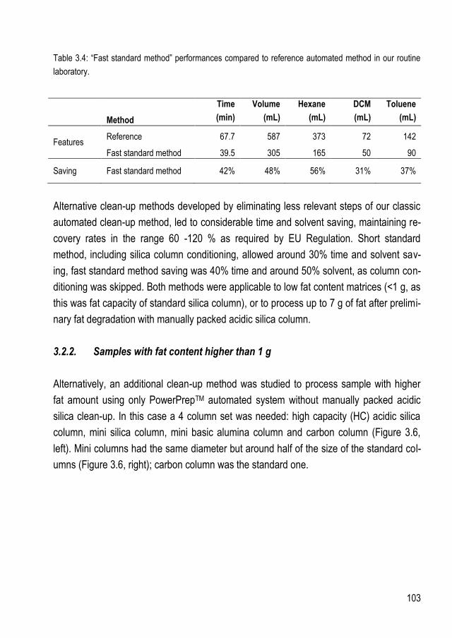
103
Table 3.4: “Fast standard method” performances compared to reference automated method in our routine
laboratory.
Alternative clean-up methods developed by eliminating less relevant steps of our classic
automated clean-up method, led to considerable time and solvent saving, maintaining re-
covery rates in the range 60 -120 % as required by EU Regulation. Short standard
method, including silica column conditioning, allowed around 30% time and solvent sav-
ing, fast standard method saving was 40% time and around 50% solvent, as column con-
ditioning was skipped. Both methods were applicable to low fat content matrices (<1 g, as
this was fat capacity of standard silica column), or to process up to 7 g of fat after prelimi-
nary fat degradation with manually packed acidic silica column.
3.2.2. Samples with fat content higher than 1 g
Alternatively, an additional clean-up method was studied to process sample with higher
fat amount using only PowerPrepTM automated system without manually packed acidic
silica clean-up. In this case a 4 column set was needed: high capacity (HC) acidic silica
column, mini silica column, mini basic alumina column and carbon column (Figure 3.6,
left). Mini columns had the same diameter but around half of the size of the standard col-
umns (Figure 3.6, right); carbon column was the standard one.
Method
Time
(min)
Volume
(mL)
Hexane
(mL)
DCM
(mL)
Toluene
(mL)
Features Reference 67.7 587 373 72 142
Fast standard method 39.5 305 165 50 90
Saving Fast standard method 42% 48% 56% 31% 37%

104
Figure 3.6: (left) 4 column setup used in this part of the work. (Right) mini column size compared to stan-
dard columns.
HC acidic silica column from FMS contains 45 g of 44% acidic silica so its fat capacity is
up to 4 grams. This column has Teflon chips on the top (Figure 3.7) to disperse the sam-
ple avoiding rapid exothermic fat oxidation on silica surface. Indeed, in case of rapid oxi-
dation fact degradation by-products could form agglomerates, being lipophilic compound
in a polar environment, and generate backpressure.
Figure 3.7: Top of the high capacity acidic silica column, equipped with Teflon chips
The method, using 4 column set, was called “Jumbo method” because of the dimension
of HC silica column. Such column set was chosen for a double purpose: first, to replace
our manual acidic silica column with similar column integrated in a whole automated sys-
tem; second, to test if standard column size can be reduced to mini column size, espe-
cially alumina column. This design in fact promoted acidic lipid degradation in the jumbo
column, pH regulation in the multilayer mini silica, and final fractionation in alumina and
carbon column.
The clean-up program was based on previous studies in our laboratory (Focant and De
Pauw, 2002) and did not include conditioning step in view of the previous results.
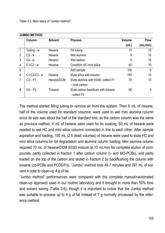
105
Table 3.5: Main steps of “Jumbo method”.
The method started filling tubing to remove air from the system. Then 6 mL of hexane,
half of the volume used for standard columns, were used to wet mini alumina column
since its size was about the half of the standard one; as the carbon column was the same
as previous method, 6 mL of hexane were used for its soaking; 60 mL of hexane were
needed to wet HC and mini silica columns connected in line to each other. After sample
aspiration and loading, 150 mL (2.5 dead volumes) of hexane were used to elute HC and
mini silica columns for fat degradation and alumina column loading. Mini alumina column
required 70 mL of hexane/DCM 50/50 mixture at 10 mL/min for complete elution of com-
pounds, partly collected in fraction 1 after carbon column (I- and MO-PCBs), and partly
loaded on the top of the carbon and eluted in fraction 2 by backflushing the column with
toluene (co-PCBs and PCDD/Fs). “Jumbo” method took 48.7 minutes and 397 mL of sol-
vent in total to clean-up 4 g of fat.
“Jumbo method” performances were compared with the complete manual+automated
clean-up approach used in our routine laboratory and it brought to more than 50% time
and solvent saving (Table 3.6), though it is important to notice that the Jumbo method
was suitable to process up to 4 g of fat instead of 7 g normally processed by the refer-
ence method.
JUMBO METHOD
Column Solvent Process Volume
(mL)
Flow
(mL/min)
1 Tubing - w Hexane Fill tubing 15 10
2 C3 - w Hexane Wet alumina 6 10
3 C4 - w Hexane Wet carbon 6 10
4 C1/C2 - w Hexane Condition HC-mini silica 60 10
5 Add sample 100 5
6 C1/C2/C3 - w Hexane Elute silica with hexane 150 10
7 C3 – F1 Hexane/DCM Elute alumina with 50/50, collect F1
– load carbon
70 10
8 C4 – F2 Toluene Elute carbon backflush with toluene
- collect F2
90 5
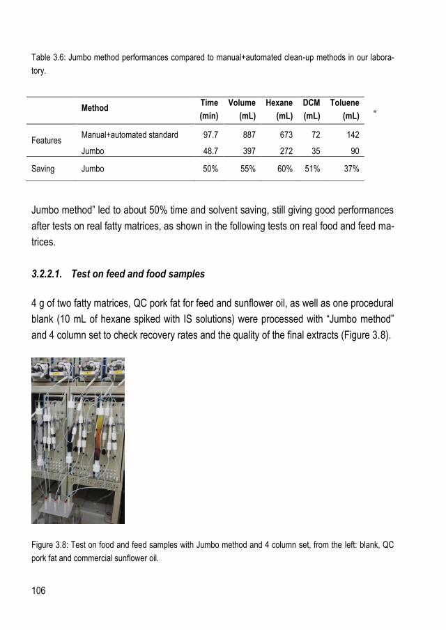
106
Table 3.6: Jumbo method performances compared to manual+automated clean-up methods in our labora-
tory.
“
Jumbo method” led to about 50% time and solvent saving, still giving good performances
after tests on real fatty matrices, as shown in the following tests on real food and feed ma-
trices.
3.2.2.1. Test on feed and food samples
4 g of two fatty matrices, QC pork fat for feed and sunflower oil, as well as one procedural
blank (10 mL of hexane spiked with IS solutions) were processed with “Jumbo method”
and 4 column set to check recovery rates and the quality of the final extracts (Figure 3.8).
Figure 3.8: Test on food and feed samples with Jumbo method and 4 column set, from the left: blank, QC
pork fat and commercial sunflower oil.
Method
Time
(min)
Volume
(mL)
Hexane
(mL)
DCM
(mL)
Toluene
(mL)
Features Manual+automated standard 97.7 887 673 72 142
Jumbo 48.7 397 272 35 90
Saving Jumbo 50% 55% 60% 51% 37%

107
Samples were diluted in 60 mL of hexane in order to decrease their viscosity and to dis-
perse the fat to reduce exothermic oxidation on the acidic silica column. After wetting the
column and checking for leaks (steps from 1 to 4 in Table 3.5), samples entered the sys-
tem by automated aspiration and were loaded on the high capacity and mini silica col-
umns with hexane at 10 mL/min (step 6). As the sample interacted with the sorbent, lipid
oxidation occurred and the sorbent turned darker. As shown in Figure 3.8, pork fat lipid
degradation (central sample) seemed to occur faster than sunflower oil oxidation (sample
on the right), as the sorbent was very dark until the middle of the column, whereas for
sunflower oil fat degradation seemed to be slower as sorbent looked brownish for all col-
umn length. A possible explanation to this experimental evidence can be found in the dif-
ferent composition of these matrices, in particular in triglyceride composition, reported in
Table 3.7 (O'Brien, 2009).
Table 3.7: Triglyceride composition of pork fat and sunflower oil.
Sunflower oil is mainly constituted by unsaturated triglyceride, unlike pork fat which con-
tains more saturated triglycerides. One hypothesis to explain why sunflower oil oxidation
is slower than lard oxidation, is the presence of competitive reactions acid catalyzed oc-
curring instead of fat hydrolysis. In acid media, in fact, water and alcohol can add to dou-
ble bond of unsaturated chains of triglycerides to form alcohols and ethers (electrophilic
addition), which are further oxidized but in a second step. According to this, lard oxidation
is faster because of the presence of less unsaturated chains for competitive reaction.
Matrix Triglyceride composition, % Typical Range
Pork fat (lard) SSS Trisaturatedl
SSU Disaturatedl
UUS Monosaturated
UUU Unsaturated
Lard composition is variable
and it depends on animal diet.
Only ranges can be defined
2 to 5
25 to 35
50 to 60
10 to 30
Sunflower oil SSS Trisaturatedl
SUS Disaturatedl
SSU Disaturated
SUU Monosaturated
UUU Unsaturated
0.3
2.9
0.2
26.6
70.2
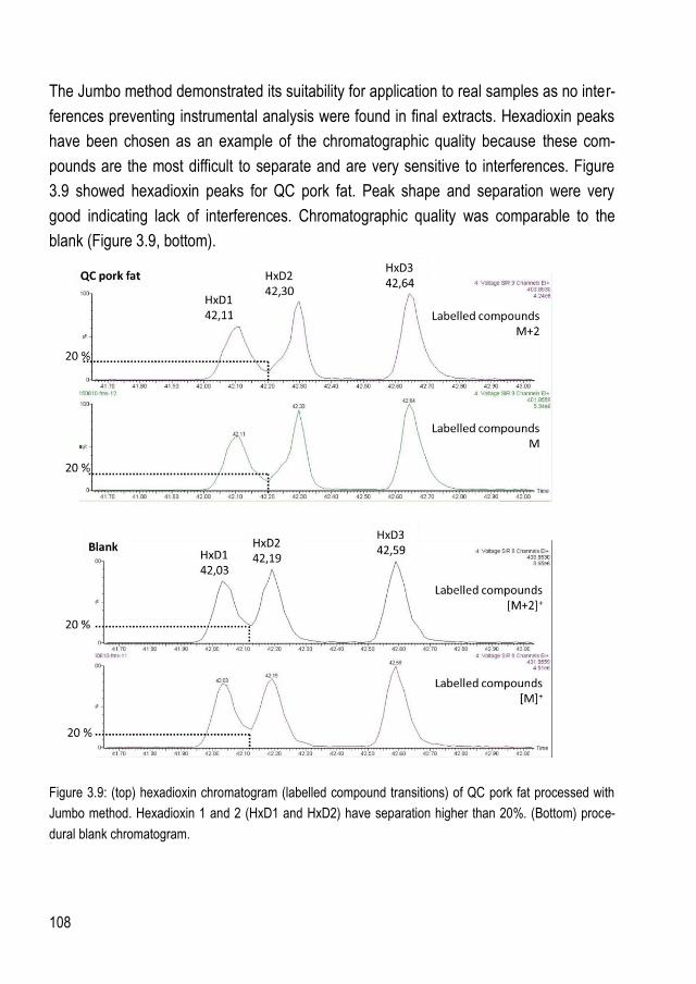
108
The Jumbo method demonstrated its suitability for application to real samples as no inter-
ferences preventing instrumental analysis were found in final extracts. Hexadioxin peaks
have been chosen as an example of the chromatographic quality because these com-
pounds are the most difficult to separate and are very sensitive to interferences. Figure
3.9 showed hexadioxin peaks for QC pork fat. Peak shape and separation were very
good indicating lack of interferences. Chromatographic quality was comparable to the
blank (Figure 3.9, bottom).
Figure 3.9: (top) hexadioxin chromatogram (labelled compound transitions) of QC pork fat processed with
Jumbo method. Hexadioxin 1 and 2 (HxD1 and HxD2) have separation higher than 20%. (Bottom) proce-
dural blank chromatogram.
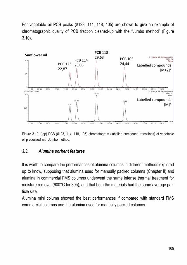
109
For vegetable oil PCB peaks (#123, 114, 118, 105) are shown to give an example of
chromatographic quality of PCB fraction cleaned-up with the “Jumbo method” (Figure
3.10).
Figure 3.10: (top) PCB (#123, 114, 118, 105) chromatogram (labelled compound transitions) of vegetable
oil processed with Jumbo method.
3.3. Alumina sorbent features
It is worth to compare the performances of alumina columns in different methods explored
up to know, supposing that alumina used for manually packed columns (Chapter II) and
alumina in commercial FMS columns underwent the same intense thermal treatment for
moisture removal (600°C for 30h), and that both the materials had the same average par-
ticle size.
Alumina mini column showed the best performances if compared with standard FMS
commercial columns and the alumina used for manually packed columns.

110
Table 3.8: Comparison between the performances of basic alumina used in the method with manually
packed columns, and in the method with commercial mini columns.
For manually packed columns in Chapter II, 7 cm x 1.7 mm ID glass tube was filled with
10 g of basic alumina, which were able to hold compounds after 175 mL of hexane flow-
ing at 7 mL/min. In the present case, commercial mini columns contained 6 g of basic
alumina in a PTFE 8 cm x 0.9 mm ID tube and were able to hold compounds despite 150
mL flowing of hexane at 10 mL/min. On the other hand, standard alumina column con-
tained 11 g of sorbent in a PTFE 16 cm x 0.9 mm ID column and it was flushed with 90
mL of hexane at 10 mL/min (Table 3.8).
Alumina mini columns showed the best performances among the alumina columns stud-
ied, as the ratio between the amount of sorbent in the column and the amount of solvent
flushing the column with hexane (during fat degradation on the silica column) was the
smallest (0.04). From these results, one could think that sorbent amount in the standard
FMS column is exceeding the necessary quantity, as mini columns, despite the appar-
ently low amount, showed performances suitable for the scope, even in hard conditions.
Moreover, mini commercial column seemed to be very active also in comparison with
alumina in the manually packed columns, despite the smaller sorbent amount and the
higher solvent flow.
Parameter Alumina in the
manually packed
column
Alumina in the
standard
commercial column
Alumina in the
mini
commercial column
Amount 10 g 11 g 6 g
Column 7 cm x 1.7 mm ID 16 cm x 0.9 mm ID 8 cm x 0.9 mm ID
Hexane amount 175 mL 90 mL 150 mL
Solvent flow 7 mL/min 10 mL/min 10 mL/min
Ratio sorbent/solvent 0.058 0.122 0.04
111
4. Conclusions
Alternative clean-up approaches were developed for the PowerPrepTM system from FMS
with the aim of having high throughput method for dioxin analysis with time, solvent and
global cost reduction. Approaches were based on our validated clean-up method consist-
ing of a preliminary lipid digestion with a manually packed acidic silica column, followed
by automated clean-up with PowerPrepTM equipped with a 3 column set: standard ABN
silica, alumina and carbon column. “Short” and “fast standard methods” used the same
column set and were suitable for low fat content samples (< 1 g) or they had to come after
a preliminary acidic digestion with manually packed acidic silica column to have fat capac-
ity of up to 7 g. New methods were designed from our routine automated method remov-
ing less crucial steps, namely column washing/conditionings and tubing washing. Silica,
alumina and carbon column elution profiles were studied to assess minimum solvent
amount for column elution. “Fast standard method” showed also that initial silica column
conditioning could be skipped without affecting final recoveries and extract quality. Alter-
native automated approaches allowed from 30 to 50% saving in terms of solvent and
time.
“Jumbo method” was developed as a fully automated alternative to our entire clean-up
procedure including the manual and the automated steps. Jumbo method used 4 column
set on the PowerPrepTM: high capacity acidic silica column, mini ABN silica, mini alumina
and carbon column, for a total fat capacity of up to 4 g and about 50% solvent and time
saving in comparison to our whole clean-up procedure. After development, the method
was tested on pork fat QC and commercial vegetable oil to check the quality of the final
extracts, and it demonstrated to be suitable for trace level measurement of dioxins and
PCBs. Standar and mini FMs alumina column performances were compared and mini
column demonstrated to be suitable for the fractionation of dioxins, furans and PCBs
processing up to 4 g of fat. Likely, standard FMS alumina column is oversized and it could
be replaced by mini column with solvent and time saving.
112
Bibliography
ABAD, E., SAULÓ, J., CAIXACH, J. & RIVERA, J. 2000. Evaluation of a new automated cleanup system for the analysis of polychlorinated dibenzo-p-dioxins and dibenzofurans in environmental samples. Journal of Chromatography A, 893, 383-391.
FOCANT, J. F. & DE PAUW, E. 2002. Fast automated extraction and clean-up of biological fluids for polychlorinated dibenzo-p-dioxins, dibenzofurans and coplanar polychlorinated biphenyls analysis. Journal of Chromatography B: Analytical Technologies in the Biomedical and Life Sciences, 776, 199-212.
FOCANT, J. F., EPPE, G., MASSART, A. C., SCHOLL, G., PIRARD, C. & DE PAUW, E. 2006. High-throughput biomonitoring of dioxins and polychlorinated biphenyls at the sub-picogram level in human serum. Journal of Chromatography A, 1130, 97-107.
FOCANT, J. F., EPPE, G., PIRARD, C. & DE PAUW, E. 2001. Fast clean-up for polychlorinated dibenzo-p-dioxins, dibenzofurans and coplanar polychlorinated biphenyls analysis of high-fat-content biological samples. Journal of Chromatography A, 925, 207-221.
FOCANT, J. F., PIRARD, C. & DE PAUW, E. 2004. Automated sample preparation-fractionation for the measurement of dioxins and related compounds in biological matrices: A review. Talanta, 63, 1101-1113.
FUJITA, H., HONDA, K., HAMADA, N., YASUNAGA, G. & FUJISE, Y. 2009. Validation of high-throughput measurement system with microwave-assisted extraction, fully automated sample preparation device, and gas chromatography-electron capture detector for determination of polychlorinated biphenyls in whale blubber. Chemosphere, 74, 1069-1078.
O'BRIEN, R. 2009. Fat and oils. Formulating and processing for applications. PIRARD, C., FOCANT, J. F. & DE PAUW, E. 2002. An improved clean-up strategy for
simultaneous analysis of polychlorinated dibenzo-p-dioxins (PCDD), polychlorinated dibenzofurans (PCDF), and polychlorinated biphenyls (PCB) in fatty food samples. Fresenius' Journal of Analytical Chemistry, 372, 373-381.

113
CHAPTER IV
Based on the following publication
L’Homme B*., Calaprice C*., Calvano C.D., Zambonin C., Leardi R., Focant J.-F., (2015)
“Ultra-trace measurement of Dechloranes to investigate food as a route of human
exposure”
Chemosphere. 2015 Nov; 139:525-33. Doi: 10.1016/j.chemosphere.2015.07.043.
* These authors contributed equally to this work
1. Introduction
In this project, the main method for dioxin analysis was modified in order to integrate a
new class of compounds, Dechloranes, in the regular controls for dioxins.
This study started after the detection of Dechloranes in human blood of people from
France (Brasseur et al., 2014) even if no production site has been identified in Europe.
The study was aimed to determine the main route of human exposure to these com-
pounds and the investigation was started from food, as it is the main route of exposure to
dioxins.
In this part of the work of thesis, an analytical method from sample preparation to instru-
mental detection with GC-MS/MS Triple Quad was developed to allow the assessment of
Dechlorane levels in food and feed, with the aim of investigating the contribute of food
consumption to human exposure to these chemicals. The analytical approach was based
on the fully validated method using isotope dilution (ID) and GC-MS/MS Triple quad in-
strument for the measurement of dioxins in food and feed at the low pg level under the
European Legislation (L'Homme et al., 2015) with the aim of allowing simultaneous
analysis of dioxins and Dehcloranes during regular food safety controls. Instrumental pa-
rameters were optimized to reach very high sensitivity at ppb levels. For this purpose,
programmed temperature vaporizing (PTV) injector in solvent vent mode for large volume
injection (LVI) was used; experimental design, in particular, full factorial design (FFD) and
114
face-centered design (FCD) were used to select optimum values for the three most rele-
vant factors for us, such as vent flow, vent pressure, and vent temperature. On the MS
side, specific multiple reaction monitoring (MRM) transitions were selected from
Dechlorane fragmentation pattern, that followed a retro Diels-Alder reaction of the no-
rbornene moiety of the molecule (Brasseur et al., 2012; Shen et al., 2012). The method
was validated following the applicable criteria of the EU Regulation for dioxins, as dedi-
cated regulation for Dechloranes is not yet available and MLs have not been assessed.
2. Dechlorane structures
Dechloranes are a family of organo-chlorinated compounds sharing a bicyclo [2,2,1] hep-
tene structure, resulting from a Diels–Alder reaction between one or two molecules of
hexachlorocyclopentadiene (HCCPD) with various cyclic dienophiles. The first of these
compounds was Mirex, also called Dechlorane, which is included in the Annex A of the
list of POPs drawn up during the Stockholm Convention (www.pops.int/), including chemi-
cals whose production and use have to be eliminated because of their intrinsic toxicity. In
fact, since 1978, Mirex is no longer made or used in the United States, but it was exten-
sively used in the 1960s and 1970s as a pesticide to control fire ants, and also as a flame
retardant additive under the trade name Dechlorane® in plastics, rubber, paint, paper, and
electrical goods from 1959 to 1972, because it does burn easily (ATSDR, 2000). Since
that time several studies were carried out on Mirex, highlighting its toxicity and negative
effects on biota and humans (Keisr, 1978).
After Mirex was banned, structural similar compounds were synthetized to replace Mirex
since no restriction was put on them. Dechlorane compounds are Dechlorane Plus, syn-
and anti-isomer (DP, C18H12Cl12), Dechlorane 602 (Dec 602, C14H4Cl12O), Dechlorane
603 (Dec 603, C17H8Cl12), Dechlorane 604 (Dec 604, C13H4Br4Cl6) and Chlordene Plus
(CP, C15H6Cl12) (Figure 4.1) (Inchem, 1984).

115
Mirex
Figure 4.1: Dechlorane structures
116
3. Dechlorane sources, environmental and biological contamination
DP syn- and anti-isomers are currently produced by OxyChem in Niagara Falls, New
York, and by Anpon in Huai’an in China (Sverko et al., 2011). The isomers in the technical
mixture are in a ratio 1:3 for the anti isomer, that is thermodynamically more stable. DPs
are currently used as flame retardants in electrical hard plastic connectors in televisions
and computer monitors, wire coating, and furniture (Betts, 2006). Several studies showed
the presence of DP isomers and other Dechloranes in the environmental (Hoh et al.,
2006, Shen et al., 2010, Jia et al., 2011, Peng et al., 2014) and in biota samples (Guerra
et al., 2011, Kim et al., 2014, Sühring et al., 2015), highlighting POP features of low solu-
bility in water, chemical and physical stability, biopersistence and hence long range trans-
port, bioaccumulation and biomagnification in the food chain. Very recent human biomoni-
toring studies have reported levels at the ng/g lipid in human serum from Norway
(Cequier et al., 2013) and France (Brasseur et al., 2014), as well as in breast milk from
Canada (Zhou et al., 2014).
4. Materials and methods
4.1. Chemicals and consumables
Solvents (hexane, dichloromethane, toluene, methanol) were Picograde® reagents (LGC
Promochem, Wesel, Germany). All solvent batches were tested for investigated analyte
contamination before use. Nonane and dodecane puriss analytical-reagent grade stan-
dard for GC were purchased from Fluka (Steinheim, Germany). Water was obtained from
a Milli-Q Ultrapure water purification system (Millipore, Brussels, Belgium). Ethanol, am-
monium hydroxide solution 28-30% and ethyl ether were purchased from Sigma Aldrich
(St. Louis, MO, USA). Silica gel was purchased from Macherey-Nagel (Macherey-Nagel
GmbH & Co KG, Düren, Germany). Disposable PTFE columns for the automated clean-
up were obtained from Fluid Management Systems (FMS Inc., Waltham, MA, USA).
Chromatographic pure grade helium gas, 99.9999% alphagaz 2 was purchased from Air
Liquide (Paris, France). Technical N27 grade liquid CO2 was used for PTV cooling (Air
117
Liquide, Paris, France). Sodium sulphate and diatomaceous earth were purchased from
VWR International (Radnor, PA, USA).
Dechlorane quantitation was performed with Isotope Dilution (ID) technique, using the la-
belled internal standards available at the moment of the work. DP syn 13C10-labelled inter-
nal standard and Dec 602 13C10-labelled internal standard, as well as DP syn and DPanti
standards were supplied by Cambridge Isotope Laboratories (CIL, Andover, MS, USA).
Mirex standard was purchased from Cluzeau Info Labo (France); Dec 602, Dec 603 and
Dec 604 standards were purchased from Toronto Research Chemical Inc. (Toronto, ON,
Canada); CP standard was bought from Wellington Laboratories (Guelph, ON, Canada).
DP syn 13C10-labelled internal standard was used for the quantitation of DP isomers, while
Dec 602 13C10-labelled internal standard was used for Mirex, Dec 602, Dec 603, Dec 604
and CP based on retention time proximity. The EC-1414 solution of 13C12-labelled PCB 80
was purchased from CIL and used as recovery standard for all the compounds. Calibra-
tion curves were prepared from stock standard solutions at 100 µg/mL and consisted in 5
to 7 calibration points.
4.2. Samples
After method development with standard solutions, a total of 88 samples were analysed
to assess average levels in food and feed. Sample matrices consisted in chicken, pork,
pure animal fat, salmon, milk, eggs, vegetable oil for feed, feed additives, and corn. 77
samples out 88 were randomly selected from samples entering our ISO17025 accredited
laboratory for monitoring controls on PCDD/Fs and PCBs; the remaining 11 samples (5
salmons and 6 chickens) were collected from regular shops and supermarkets in the area
of Liege, Belgium, in January 2015, to have a complete overview of several food matri-
ces. During the study, 16 procedural blanks were also analysed.
4.3. Sample preparation: extraction and clean up
Sample preparation procedure, extraction and clean-up included, was the same used for
polychlorodibenzo-p-dioxin (PCDD), polychloro-dibenzofuran (PCDF), and polychlorobi-
phenyl (PCB) analysis in our laboratory. Detailed description of the procedures for all ma-
118
trix typologies is out of the scope of this report and it has been already published (Focant
et al., 2001, Focant et al., 2006, Pirard et al., 2002). Briefly, for all the matrices (except al-
ready pure fat) fat extraction was required because of Dechlorane lipophilicity (as diox-
ins), and it was performed by Accelerated Solvent Extraction (ASETM 350, Dionex,
Thermo Fisher Scientific). Only for milk, liquid-liquid extraction was required and the pro-
cedure is reported in Chapter 2 of this thesis. Samples were spiked with internal stan-
dards before fat extraction for salmon and feed, and directly on the extracted fat for the
other matrices, according to the guidelines of the EU Regulation for dioxin analysis, as no
guidelines are available for Dechloranes. Afterwards, samples underwent a double step
clean-up in the same framework as dioxins and PCBs: first step was a manually packed
acidic silica column for intense lipid digestion, and second step was automated clean-up
and fractionation of dioxins and PCBs with PowerPrepTM automated system (FMS Inc,
Waltham, USA), equipped with standard ABN silica, alumina and carbon column (Focant
et al., 2004). As for PCDD/F and PCB classical clean-up, two fractions were collected and
sent to instrumental analysis. Dechloranes were collected in fraction 1 (F1) with non-
planar species collected by forward elution of the alumina-carbon column with hex-
ane/DCM 50/50 mixture. This fraction was injected for Dechlorane analysis after evapora-
tion of solvents in a dedicated tube using a sensor-equipped TurboVap II Workstation
(Caliper Life Science, Teraflene, Belgium) and after subsequent evaporation in GC vials
containing nonane (90 µL) as a keeper using a RapidVap (Labconco, Kansas City, MO,
USA). The 13C12-labelled PCB 80 recovery standard was added before instrumental
analysis. Blanks were processed following the same procedure of their corresponding
matrix according to the Table 4.1. Some matrices had the same procedural blank be-
cause followed the same extraction procedure.

119
Table 4.1: Procedural blanks for several food and feed matrices in our laboratory
Corresponding matrix Blank number
Chicken
Pork
Egg
Pure fat
Salmon
Vegetable oil (for feed)
10 mL of hexane 9
Milk 80 mL Ultrapure water 3
Feed additives
Corn
Na2SO4 and diatomaceous earth mixture
4
Total 16
4.4. GC-MS/MS conditions
Instrumental analysis was carried out with GC-MS/MS Triple Quad instrument from
Agilent (Palo Alto, CA, USA), namely a 7890G gas chromatographer coupled with a
7000C Triple Quadrupole mass spectrometer. The GC was equipped with a programma-
ble temperature vaporization (PTV) inlet, and a 7693A automated liquid sampler (ALS). 5
µL out of 100 µL of the final purified extract were injected into the PTV inlet operating in
solvent vent mode and cooled by liquid CO2. The inlet temperature program and solvent
vent parameters were optimized by means of an experimental design and were: inlet ini-
tial temperature of 45°C for 1.3 min, ramped up at 720°C/min to 320°C and hold until the
end of the run; vent flow was set at 120 mL/min at vent pressure of 10.5 psi. Purge flow
was set to 1200 mL/min after 5 min to insure complete evacuation of the inlet and prevent
from possible memory effects. All the computations and graphs were performed using
multiple linear regression routines written in Matlab (Mathworks Inc., Natrick, USA). The
GC column was the same used for dioxin analysis, namely an Agilent DB-5ms ultra inert
(60 m x 0.25 mm x 0.25 µm), in order to allow Dechlorane analysis when doing routine
controls for dioxins and PCBs without changing instrumental layout. The GC oven tem-
perature program was characterised by a sharp ramp because of Dechlorane high mo-
lecular weight: start at 140°C for 2.6 min, ramp at 100°C/min to 320°C and hold for 21.1
min (total run time of 25.5 min). The transfer line temperature was held at 320°C. On the

120
MS side, electron ionization (EI) ion source at 70eV energy and temperature of 280°C
was used. Temperature of the quadrupoles was set at 150°C and multiple reaction moni-
toring (MRM) transitions were recorded at ‘wide’ mass resolution, which means 1.2 Da on
the Agilent software. Ultrapure Nitrogen at 1.5 mL/min and Helium at 2.25 mL/min were
used as collision gas and quench gas in the collision cell, respectively. Dwell times were
selected during method optimization to increase the sensitivity as much as possible and
to adjust the acquisition frequency to get ten data points per peak. Calibration and auto-
tune were performed in the EI high sensitivity mode. Retention time locking was per-
formed with PCB 105 allowing change and reinstallation of the column while keeping re-
producible retention times. Mass Hunter version B.07.00 was used for acquisition and
quantitative analysis.
5. Results and discussion
5.1. Sample clean-up
The study was aimed to the development of a multi-analyte procedure that included
Dechloranes during regular controls for dioxins and PCBs, as from previous experience in
our laboratory, it was known that typical dioxin sample preparation procedures were us-
able for Dechlorane measurements in serum and that Dechloranes could be collected in
fraction 1 together with non-planar compounds (Brasseur et al., 2014).
Due to the lipophilic nature of Dechloranes, fat extraction procedures for each matrix were
maintained the same as dioxin analysis. For sample clean-up, matrices with fat amount
higher than blood were processed and stronger lipid acidic degradation was required. So,
our routine sample clean-up approach, manual and automated stages, was checked step-
by-step with recovery experiments, to investigate possible degradation of Dechlorane
compounds under such acidic treatment. Figure 4.2 reports the detailed fractionation
study where Dechlorane recovery rates were measured after each clean-up step. 10 mL
of hexane spiked with 100 pg/µL mixture of all the compounds were cleaned up following
the procedure one step at a time; eluate was collected and evaporated to approximately
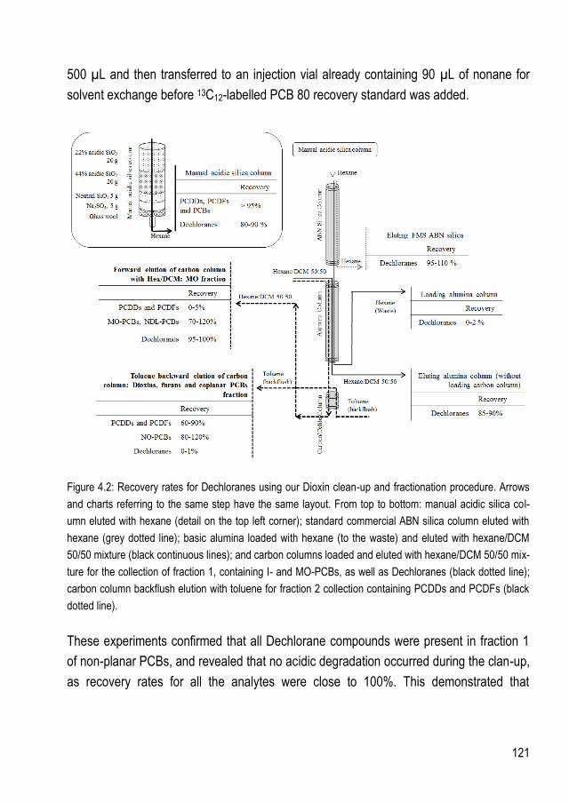
121
500 µL and then transferred to an injection vial already containing 90 µL of nonane for
solvent exchange before 13C12-labelled PCB 80 recovery standard was added.
Figure 4.2: Recovery rates for Dechloranes using our Dioxin clean-up and fractionation procedure. Arrows
and charts referring to the same step have the same layout. From top to bottom: manual acidic silica col-
umn eluted with hexane (detail on the top left corner); standard commercial ABN silica column eluted with
hexane (grey dotted line); basic alumina loaded with hexane (to the waste) and eluted with hexane/DCM
50/50 mixture (black continuous lines); and carbon columns loaded and eluted with hexane/DCM 50/50 mix-
ture for the collection of fraction 1, containing I- and MO-PCBs, as well as Dechloranes (black dotted line);
carbon column backflush elution with toluene for fraction 2 collection containing PCDDs and PCDFs (black
dotted line).
These experiments confirmed that all Dechlorane compounds were present in fraction 1
of non-planar PCBs, and revealed that no acidic degradation occurred during the clan-up,
as recovery rates for all the analytes were close to 100%. This demonstrated that
122
Dechlorane analysis can be integrated in a multi-analyte method including already dioxins
and PCBs, without modifying sample preparation layout.
5.2. Experimental design for optimization of PTV parameters
5.2.1. Structure of the experimental design
Since no preliminary data about Dechlorane background levels in food and feed matrices
in Europe, and no Regulation about MLs was available, a wide dynamic range including
ultra-trace levels was considered in the study. To insure method sensitivity a Design of
Experiment (DoE) was performed for the programmed temperature vaporizing (PTV) inlet,
as the first interface affecting method sensitivity. PTV inlet was working in solvent vent
mode, so initial inlet temperature (T), vent flow (VF), and vent pressure (VP) were chosen
as the most relevant factors for the experimental design, because they effected sample
transfer into the column and hence method sensitivity.
A preliminary 23 full factorial design (FFD) was performed to explore the experimental
domain and to assess a suitable model to postulate for a further more rigorous experi-
mental design investigation. According to the screening results, central point and bounda-
ries of the experimental domain were chosen. Thereafter, in this smaller domain (Table
4.2), experiments of a face-centred design (FCD) on three factors were done to calculate
the coefficients of the postulated model in Equation 1, where quadratic effects and inter-
actions between variables are taken into account.
(Eq.1)
where:
- is the experimental factor representing initial inlet temperature (T) for i=1, sol-
vent vent flow (VF) for i=2 and solvent vent pressure (VP) for i=3;
- is the factor representing the interaction between factor i and j, or the quad-
ratic factor if i=j;
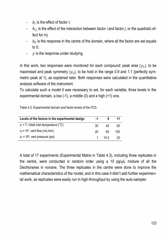
123
- is the effect of factor i;
- is the effect of the interaction between factor i and factor j, or the quadratic ef-
fect for i=j;
- is the response in the centre of the domain, where all the factor are set equals
to 0;
- is the response under studying.
In this work, two responses were monitored for each compound: peak area ( ), to be
maximised and peak symmetry ( ), to be hold in the range 0.9 and 1.1 (perfectly sym-
metric peak at 1), as explained later. Both responses were calculated in the quantitative
analysis software of the instrument.
To calculate such a model it was necessary to set, for each variable, three levels in the
experimental domain, a low (-1), a middle (0) and a high (+1) one.
Table 4.2: Experimental domain and factor levels of the FCD.
Levels of the factors in the experimental design -1 0 +1
x1 = T, initial inlet temperature (°C) 30 45 60
x2 = VF, vent flow (mL/min) 20 60 100
x3 = VP, vent pressure (psi) 1 10.5 20
A total of 17 experiments (Experimental Matrix in Table 4.3), including three replicates in
the centre, were conducted in random order using a 10 pg/µL mixture of all the
Dechloranes in nonane. The three replicates in the centre were done to improve the
mathematical characteristics of the model, and in this case it didn’t add further experimen-
tal work, as replicates were easily run in high-throughput by using the auto-sampler.

124
Table 4.3: Experimental Matrix of the Face Centered Design with 3 replicates in the center.
x1 = T x2 = VF x3 = VP
1 30 20 1
2 60 20 1
3 30 100 1
4 60 100 1
5 30 20 20
6 60 20 20
7 30 100 20
8 60 100 20
9 30 60 10.5
10 60 60 10.5
11 45 20 10.5
12 45 100 10.5
13 45 60 1
14 45 60 20
15 45 60 10.5
16 45 60 10.5
17 45 60 10.5
5.2.2. Peak area
Figure 4.3 shows the significant effects (the coefficients of the quadratic model) calcu-
lated for peak area ( and for each compound. At the explored concentration, 10
pg/µL, Dec 604 was not detectable and was therefore not represented. Significant coeffi-
cients were almost the same for all compounds, and were mostly related to temperature
( and , which had a negative quadratic effect on peak area, and to vent flow ( ),
which had a positive linear effect. Vent pressure ( ) was not statistically significant, but
close to have a significant negative linear effect for Mirex and DP syn.
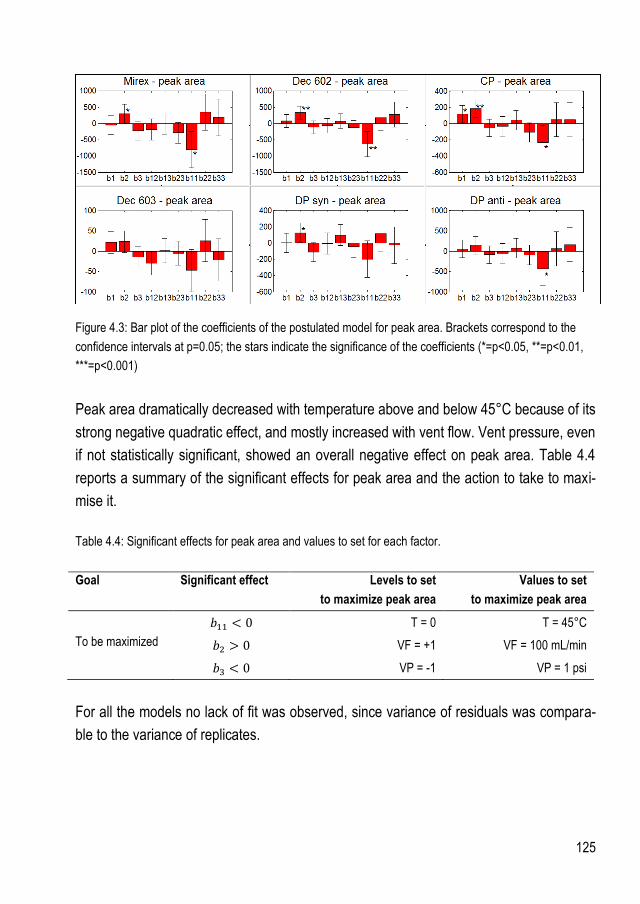
125
Figure 4.3: Bar plot of the coefficients of the postulated model for peak area. Brackets correspond to the
confidence intervals at p=0.05; the stars indicate the significance of the coefficients (*=p<0.05, **=p<0.01,
***=p<0.001)
Peak area dramatically decreased with temperature above and below 45°C because of its
strong negative quadratic effect, and mostly increased with vent flow. Vent pressure, even
if not statistically significant, showed an overall negative effect on peak area. Table 4.4
reports a summary of the significant effects for peak area and the action to take to maxi-
mise it.
Table 4.4: Significant effects for peak area and values to set for each factor.
Goal Significant effect Levels to set
to maximize peak area
Values to set
to maximize peak area
T = 0 T = 45°C
To be maximized VF = +1 VF = 100 mL/min
VP = -1 VP = 1 psi
For all the models no lack of fit was observed, since variance of residuals was compara-
ble to the variance of replicates.

126
5.2.3. Peak symmetry
Peak symmetry was calculated at 10% height of the peak as the ratio between the dis-
tance from the tail part of the peak to the centre of the apex, and from the front part of the
peak to the centre of the apex (Figure 4.4).
Figure 4.4: Calculation of peak symmetry done by the software of the instrument used in this work.
A symmetry value of 1.0 meant that the peak was balanced, whereas values lower and
higher than 1 indicated respectively peak fronting and tailing. In this work, peak symmetry
values between 0.9 and 1.1 were considered as acceptable, although the best symmetry
was reached at 1.0. This was because peak symmetry was calculated on raw experimen-
tal data without smoothing and experimental variation of the peak apex from the centre of
the peak was expected.
Figure 4.5 shows the effects calculated for peak symmetry ( ). In this case, tempera-
ture, vent flow and their interaction were significant for some analytes ( ≠ 0),
while vent pressure ( ) was almost significant (positive effect) at 95% confidence for
Mirex only.
ront)Distance(f
ail)Distance(tsymmetry
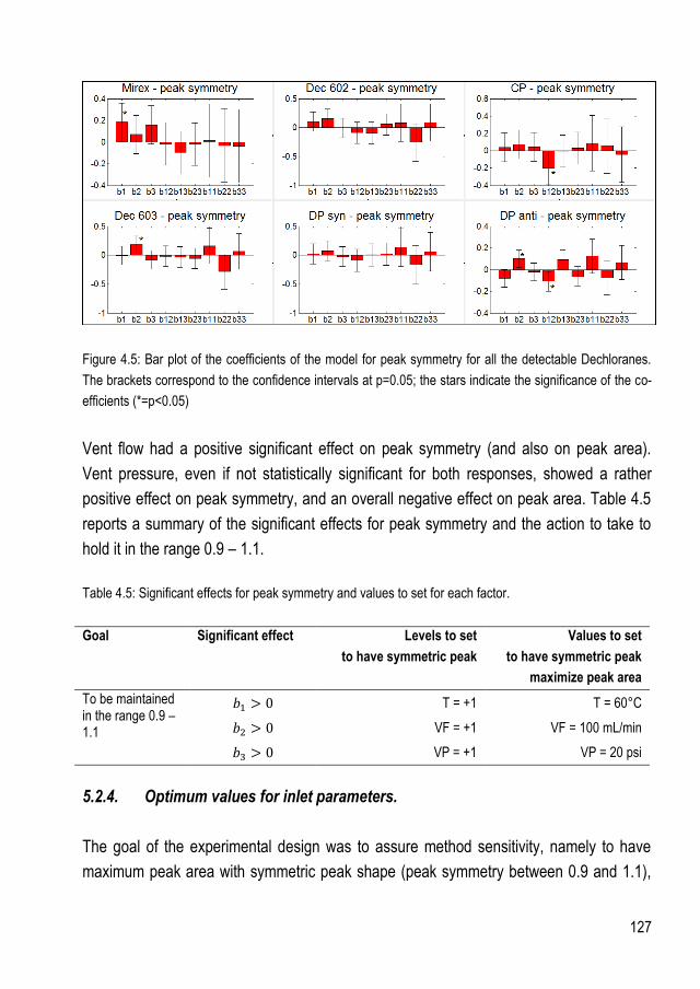
127
Figure 4.5: Bar plot of the coefficients of the model for peak symmetry for all the detectable Dechloranes.
The brackets correspond to the confidence intervals at p=0.05; the stars indicate the significance of the co-
efficients (*=p<0.05)
Vent flow had a positive significant effect on peak symmetry (and also on peak area).
Vent pressure, even if not statistically significant for both responses, showed a rather
positive effect on peak symmetry, and an overall negative effect on peak area. Table 4.5
reports a summary of the significant effects for peak symmetry and the action to take to
hold it in the range 0.9 – 1.1.
Table 4.5: Significant effects for peak symmetry and values to set for each factor.
Goal Significant effect Levels to set
to have symmetric peak
Values to set
to have symmetric peak
maximize peak area
To be maintained in the range 0.9 – 1.1
T = +1 T = 60°C
VF = +1 VF = 100 mL/min
VP = +1 VP = 20 psi
5.2.4. Optimum values for inlet parameters.
The goal of the experimental design was to assure method sensitivity, namely to have
maximum peak area with symmetric peak shape (peak symmetry between 0.9 and 1.1),
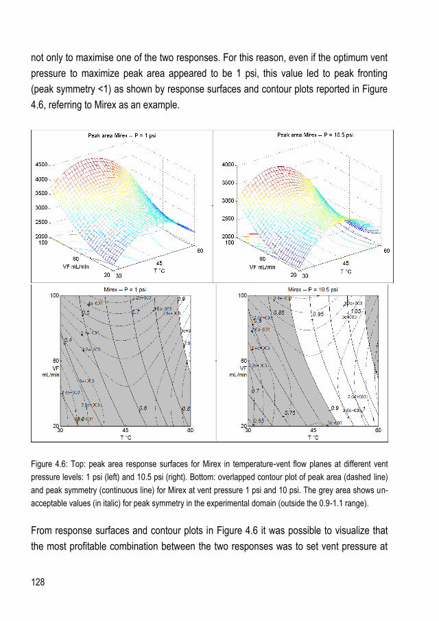
128
not only to maximise one of the two responses. For this reason, even if the optimum vent
pressure to maximize peak area appeared to be 1 psi, this value led to peak fronting
(peak symmetry <1) as shown by response surfaces and contour plots reported in Figure
4.6, referring to Mirex as an example.
Figure 4.6: Top: peak area response surfaces for Mirex in temperature-vent flow planes at different vent
pressure levels: 1 psi (left) and 10.5 psi (right). Bottom: overlapped contour plot of peak area (dashed line)
and peak symmetry (continuous line) for Mirex at vent pressure 1 psi and 10 psi. The grey area shows un-
acceptable values (in italic) for peak symmetry in the experimental domain (outside the 0.9-1.1 range).
From response surfaces and contour plots in Figure 4.6 it was possible to visualize that
the most profitable combination between the two responses was to set vent pressure at

129
10.5 psi (intermediate level in the domain), vent flow at 100 mL/min (highest level in the
domain) and temperature at 45°C (intermediate level in the domain) (Table 4.6)
Table 4.6: Optimum values of the factors to maximise peak area of symmetric peaks.
Peak area Peak symmetry Optimum values
T = 45°C T = 60°C T = 45°C
VF = 100 mL/min VF = 100 mL/min VF = 100 mL/min
VP = 1 psi VP = 20 psi VP = 10.5 psi
To go further, from the peak area response curves of Figure 4.6, it was evident that peak
area might increase even more outside the experimental domain when increasing vent
flow, while still keeping vent pressure at 10.5 psi for peak symmetry. So, three replicates
at a vent flow of 120 mL/min (outside the experimental domain), temperature at 45°C and
vent pressure at 10.5 psi were recorded to check whether or not the response increased
significantly in the expected direction. Indeed, the peak area in these conditions was sta-
tistically higher (proved by a t-test) than at vent flow at 100 mL/min. At this point, even
without a full optimization but still with enough improvements using the experimental de-
sign for Dechloranes analysis, the best injection conditions were settled as vent flow (VF)
at 120 mL/min, temperature (T) at 45°C, and vent pressure (VP) at 10.5 psi.
The experimental design was useful not only to set optimum parameters for PTV inlet, but
also to highlight a memory effect in the inlet. In fact, when running replicate injections for
the experimental design, a possible memory effect emerged. To confirm this, 20 replicate
injections were done in a row and actually peak area increased for consecutive runs,
highlighting a real peak area carry over. To avoid this, inlet purge flow was increased from
100 mL/min set as default value, to 1200 mL/min (the maximum instrumental level) to in-
sure complete inlet evacuation after each run.
5.3. Instrumental method development and validation
Analytical method for Dechlorane detection was developed and validated accordingly to
the applicable criteria (Table 4.7) of the stringent EU legislation for dioxin measurement in
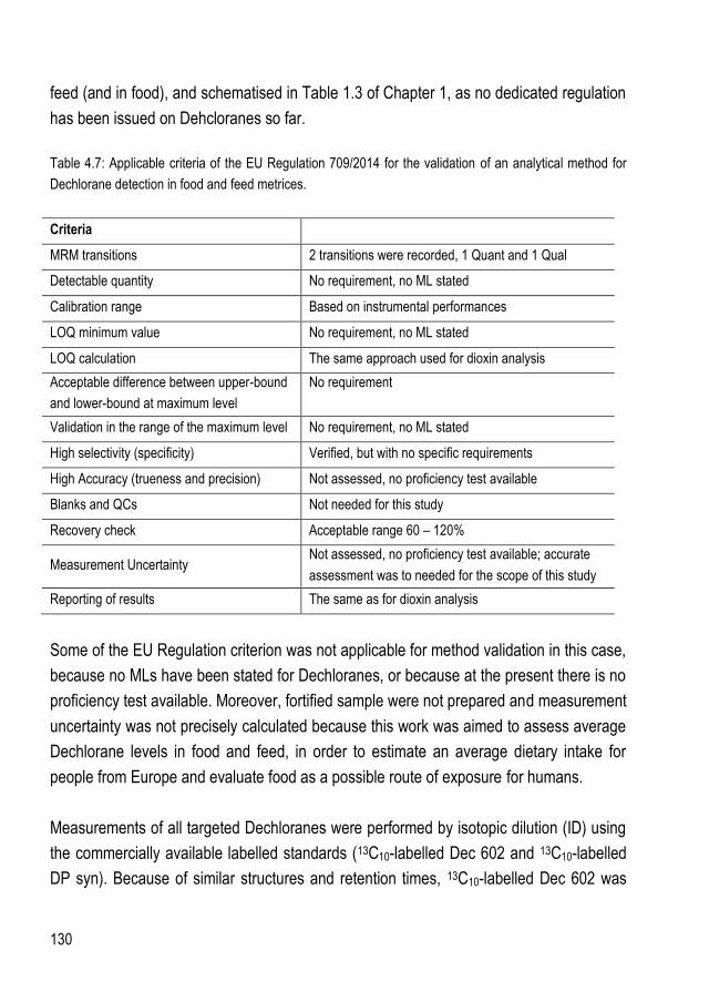
130
feed (and in food), and schematised in Table 1.3 of Chapter 1, as no dedicated regulation
has been issued on Dehcloranes so far.
Table 4.7: Applicable criteria of the EU Regulation 709/2014 for the validation of an analytical method for
Dechlorane detection in food and feed metrices.
Criteria
MRM transitions 2 transitions were recorded, 1 Quant and 1 Qual
Detectable quantity No requirement, no ML stated
Calibration range Based on instrumental performances
LOQ minimum value No requirement, no ML stated
LOQ calculation The same approach used for dioxin analysis
Acceptable difference between upper-bound
and lower-bound at maximum level
No requirement
Validation in the range of the maximum level No requirement, no ML stated
High selectivity (specificity) Verified, but with no specific requirements
High Accuracy (trueness and precision) Not assessed, no proficiency test available
Blanks and QCs Not needed for this study
Recovery check Acceptable range 60 – 120%
Measurement Uncertainty Not assessed, no proficiency test available; accurate
assessment was to needed for the scope of this study
Reporting of results The same as for dioxin analysis
Some of the EU Regulation criterion was not applicable for method validation in this case,
because no MLs have been stated for Dechloranes, or because at the present there is no
proficiency test available. Moreover, fortified sample were not prepared and measurement
uncertainty was not precisely calculated because this work was aimed to assess average
Dechlorane levels in food and feed, in order to estimate an average dietary intake for
people from Europe and evaluate food as a possible route of exposure for humans.
Measurements of all targeted Dechloranes were performed by isotopic dilution (ID) using
the commercially available labelled standards (13C10-labelled Dec 602 and 13C10-labelled
DP syn). Because of similar structures and retention times, 13C10-labelled Dec 602 was
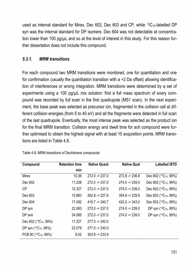
131
used as internal standard for Mirex, Dec 602, Dec 603 and CP, while 13C10-labelled DP
syn was the internal standard for DP isomers. Dec 604 was not detectable at concentra-
tion lower than 100 pg/µL and so at the level of interest in this study. For this reason fur-
ther dissertation does not include this compound.
5.3.1. MRM transitions
For each compound two MRM transitions were monitored, one for quantitation and one
for confirmation (usually the quantitation transition with a +2 Da offset) allowing identifica-
tion of interferences or wrong integration. MRM transitions were determined by a set of
experiments using a 100 pg/µL mix solution: first a full mass spectrum of every com-
pound was recorded by full scan in the first quadrupole (MS1 scan). In the next experi-
ment, the base peak was selected as precursor ion, fragmented in the collision cell at dif-
ferent collision energies (from 5 to 40 eV) and all the fragments were detected in full scan
of the last quadrupole. Eventually, the most intense peak was selected as the product ion
for the final MRM transition. Collision energy and dwell time for ach compound were fur-
ther optimised to obtain the highest signal with at least 10 acquisition points. MRM transi-
tions are listed in Table 4.8.
Table 4.8: MRM transitions of Dechlorane compounds
Compound Retention time
min
Native Quant Native Qual Labelled ISTD
Mirex 10.36 272.0 -> 237.0 273.8 -> 236.8 Dec 602 (13C10, 99%)
Dec 602 11.228 272.0 -> 237.0 274.0 -> 239.0 Dec 602 (13C10, 99%)
CP 12.327 272.0 -> 237.0 274.0 -> 239.0 Dec 602 (13C10, 99%)
Dec 603 15.883 262.8 -> 227.9 264.8 -> 229.9 Dec 602 (13C10, 99%)
Dec 604 17.092 419.7 -> 340.7 422.0 -> 343.0 Dec 602 (13C10, 99%)
DP syn 22.083 272.0 -> 237.0 274.0 -> 239.0 DP syn (13C10, 99%)
DP anti 24.085 272.0 -> 237.0 274.0 -> 239.0 DP syn (13C10, 99%)
Dec 602 (13C10, 99%) 11.227 277.0 -> 242.0
DP syn (13C10, 99%) 22.079 277.0 -> 242.0
PCB 80 (13C12, 99%) 8.02 303.9 -> 233.9
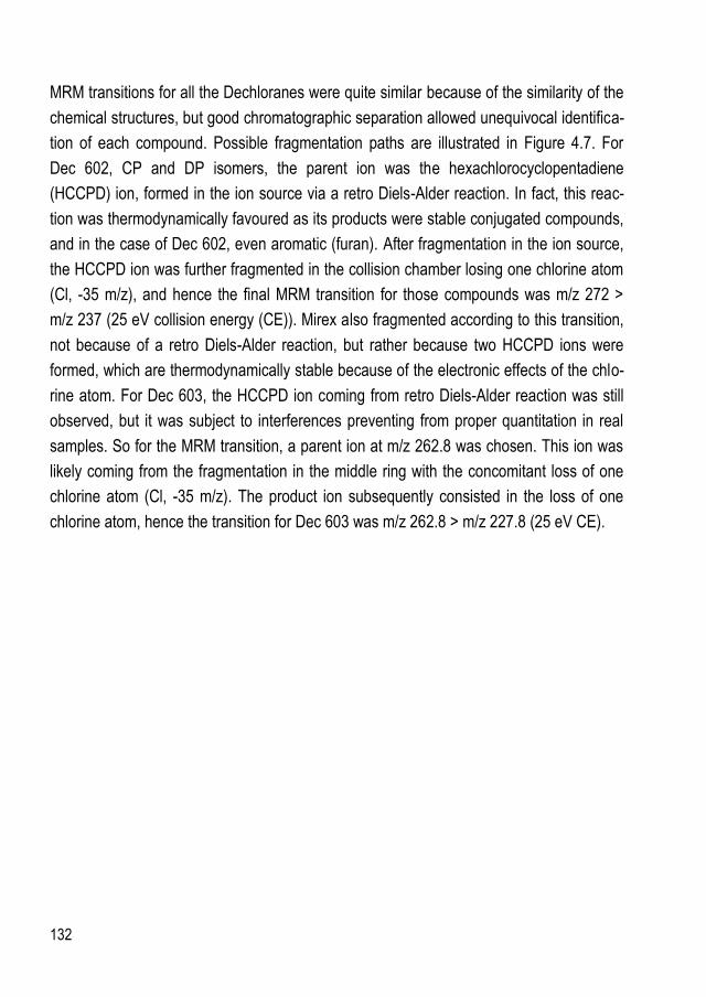
132
MRM transitions for all the Dechloranes were quite similar because of the similarity of the
chemical structures, but good chromatographic separation allowed unequivocal identifica-
tion of each compound. Possible fragmentation paths are illustrated in Figure 4.7. For
Dec 602, CP and DP isomers, the parent ion was the hexachlorocyclopentadiene
(HCCPD) ion, formed in the ion source via a retro Diels-Alder reaction. In fact, this reac-
tion was thermodynamically favoured as its products were stable conjugated compounds,
and in the case of Dec 602, even aromatic (furan). After fragmentation in the ion source,
the HCCPD ion was further fragmented in the collision chamber losing one chlorine atom
(Cl, -35 m/z), and hence the final MRM transition for those compounds was m/z 272 >
m/z 237 (25 eV collision energy (CE)). Mirex also fragmented according to this transition,
not because of a retro Diels-Alder reaction, but rather because two HCCPD ions were
formed, which are thermodynamically stable because of the electronic effects of the chlo-
rine atom. For Dec 603, the HCCPD ion coming from retro Diels-Alder reaction was still
observed, but it was subject to interferences preventing from proper quantitation in real
samples. So for the MRM transition, a parent ion at m/z 262.8 was chosen. This ion was
likely coming from the fragmentation in the middle ring with the concomitant loss of one
chlorine atom (Cl, -35 m/z). The product ion subsequently consisted in the loss of one
chlorine atom, hence the transition for Dec 603 was m/z 262.8 > m/z 227.8 (25 eV CE).

133
Figure 4.7: Possible fragmentation paths for Dechloranes when ionizing in EI at 70 eV, with subsequent
fragmentation at collision energy (CE) 25 eV.

134
5.3.2. Calibration range
The calibration range (Table 4.9) varied for each compound, based on its own dynamic
range, reproducibility at low and high level, and average response factor deviation.
Table 4.9: Calibration curve data for target Dechlorane compounds.
Compound Calibration curve range
pg/µL
Calibration
points
R2 Average
Response
factor (ARRF)*
Mirex 0.5 - 250 7 0.9997 1.4995
Dec 602 3 - 100 5 0.9993 1.2809
CP 0.5 - 100 7 0.9983 0.7754
Dec 603 0.5 - 100 7 0.9961 0.1788
DP syn 50 - 200 5 0.9995 1.0857
DP anti 3 - 200 5 0.9867 8.4338
*ARRF was the average response factor calculated on all the calibration points in the calibration range
In particular for DP syn isomer lowest calibration point was higher than for the other com-
pounds. Likely DP syn labelled standard contained native compound impurities at trace
levels, giving inaccurate concentration at very low levels.
5.3.3. Limit of Quantitation (LOQ)
Limits of quantitation were assessed with the same approach used for dioxins and PCBs
in our laboratory with Triple Quad instrument and reported in Chapter 1. So, based on the
EU Regulation, these LOQs were assessed either based on blank levels or from the in-
strumental limits of quantitation (iLOQs) when no signal was recorded in blanks. In any
case, LOQ values were kept inside the calibration range for each compound (Table 4.10).
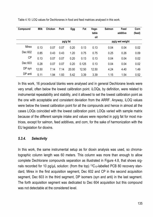
135
Table 4.10: LOQ values for Dechloranes in food and feed matrices analysed in this work.
Compound Milk Chicken Pork Egg Fat Vege-
table
oil
Salmon Feed
additive
Corn
(feed)
pg/g fat pg/g wet weight
Mirex 0.13 0.07 0.07 0.20 0.13 0.13 0.04 0.04 0.02
Dec 602 0.85 0.43 0.43 1.20 0.75 0.75 0.25 0.26 0.09
CP 0.13 0.07 0.07 0.20 0.13 0.13 0.04 0.04 0.02
Dec 603 0.28 0.07 0.07 0.20 0.125 0.13 0.04 0.04 0.02
DP syn 12.50 7.14 7.14 20.00 12.50 12.50 4.24 4.40 1.49
DP anti 5.11 1.94 1.93 5.42 3.39 3.39 1.15 1.54 0.52
In this work, 16 procedural blanks were analysed and in general Dechlorane levels were
very small, often below the lowest calibration point. iLOQs, by definition, were related to
instrumental repeatability and stability, and it allowed to set the lowest calibration point as
the one with acceptable and consistent deviation from the ARRF. Anyway, iLOQ values
were below the lowest calibration point for all the compounds and hence in almost all the
cases LOQs coincided with the lowest calibration point. LOQs varied with sample matrix
because of the different sample intake and values were reported in pg/g fat for most ma-
trices, except for salmon, feed additives, and corn, for the sake of harmonization with the
EU legislation for dioxins.
5.3.4. Selectivity
In this work, the same instrumental setup as for dioxin analysis was used, so chroma-
tographic column length was 60 meters. This column was more than enough to allow
complete Dechlorane compounds separation as illustrated in Figure 4.8, that shows sig-
nals recorded for 10 pg/µL solution: (from the top) 13C10-labelled PCB 80 recovery stan-
dard, Mirex in the first acquisition segment, Dec 602 and CP in the second acquisition
segment, Dec 603 in the third segment, DP isomers (syn and anti) in the last segment.
The forth acquisition segment was dedicated to Dec 604 acquisition but this compound
was not detectable at the considered level.
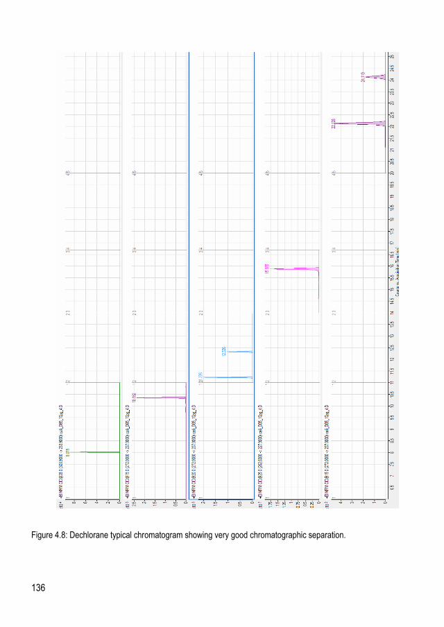
136
Figure 4.8: Dechlorane typical chromatogram showing very good chromatographic separation.

137
5.3.5. Result reporting
Also for result reporting, guidelines from the EU Regulation for dioxins were followed. In
fact, as described in the next paragraph, Dechlorane levels were reported in terms of
lower-bound (lb) and upper-bound (ub). The first approach consisted in reporting zero
whenever the experimental level measured was below the LOQ for the target compound,
hence an underestimated the measured level. On the other hand, the upper-bound ap-
proach consisted in reporting the LOQ value whenever the signal measured was below
the LOQ, even when no signal at all was recorded; this approach led to overestimation of
final measured levels. As for dioxins, also in this case, the LOQ assessment and value
was a very important parameter affecting final results.
5.4. Dechlorane levels in food and feed matrices
The analytical method was developed with the aim of assessing Dechlorane levels in food
and feed samples and average daily intake for human based on food habits of the Belgian
population. A total of 88 samples from 9 different food and feed matrices, as well as 16
blank samples were prepared following specific sample procedures. Six Dechlorane con-
centrations were measured and Dec 604 was not quantitated due to the very low re-
sponse at the level of interest. Results were calculated according to the method of report-
ing used for dioxin analysis under the EU Legislation in terms of lower-bound (lb) and up-
per-bound (ub). Table 4.11 reports Dechlorane levels calculated with the upper bound
approach on the 88 food and feed samples analysed. For the same samples, also TEQ
levels from dioxin and PCB analysis were reported, in order to demonstrate that the se-
lected samples were not particularly contaminated from dioxins and could be considered
as representative of what is actually available on the Belgian food market.
For some matrices, measured values were below LOQ, so LOQ was reported as a value
and resulting standard deviation (SD) was not computable (indicated with a dash in Table
4.11).

138
Table 4.11: Levels of selected Dechloranes measured by GC-MS/MS Triple Quad in various food and feed
matrices
Milk Chicken Pork Egg Fat
pg/g fat
Compound Mean SD Mean SD Mean SD Mean SD Mean SD
Mirex 0.50 0.24 0.11 0.07 0.21 0.25 0.21 0.02 0.43 0.68
Dec 602 0.89 0.13 0.43 - 0.43 - 1.28 0.23 0.75 -
CP 0.26 0.24 0.07 - 0.08 0.02 0.94 2.08 0.16 0.09
Dec 603 1.06 1.21 0.13 0.07 0.26 0.39 2.76 6.29 0.57 1.10
DP syn 12.50 - 7.14 - 7.14 - 20.00 - 12.50 -
DP anti 5.11 - 1.93 - 3.84 3.86 6.27 2.04 6.60 9.21
Sum DPs 17.61 - 9.08 - 10.98 3.86 26.27 2.04 19.10 9.21
Sum 6
Dechloranes 20.31 1.37 9.82 0.10 11.96 3.80 31.47 8.61 21.01 9.35
PCDD/Fs
and DL-
PCBs TEQ 1.12 0.20 0.40 0.01 0.48 0.23 0.91 0.04 0.93 0.14
Vegetable oil Salmon Feed additive Corn (feed)
pg/g fat pg/g wet weight
Compound Mean SD Mean SD Mean SD Mean SD
Mirex 0.13 - 1.98 1.43 0.07 0.10 0.01 0.46
Dec 602 0.75 - 0.31 0.10 0.26 - 0.09 -
CP 0.20 0.10 0.30 0.46 0.04 - 0.01 -
Dec 603 0.50 0.53 0.58 1.11 0.04 - 0.01 -
DP syn 12.50 - 4.24 - 4.43 0.13 1.49 -
DP anti 6.61 3.17 1.15 - 6.86 15.05 0.52 -
Sum DPs 19.11 3.17 5.39 - 11.29 15.14 2.01 -
Sum 6
Dechloranes 20.68 3.60 8.56 2.03 11.71 15.13 2.14 0.46
PCDD/Fs
and DL-
PCBs TEQ 0.20 0.00 0.62 0.61 0.39 0.33 0.20 0.00
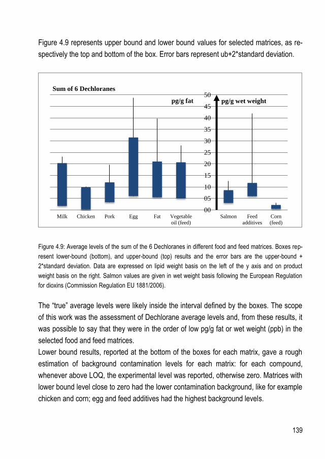
139
Figure 4.9 represents upper bound and lower bound values for selected matrices, as re-
spectively the top and bottom of the box. Error bars represent ub+2*standard deviation.
Figure 4.9: Average levels of the sum of the 6 Dechloranes in different food and feed matrices. Boxes rep-
resent lower-bound (bottom), and upper-bound (top) results and the error bars are the upper-bound +
2*standard deviation. Data are expressed on lipid weight basis on the left of the y axis and on product
weight basis on the right. Salmon values are given in wet weight basis following the European Regulation
for dioxins (Commission Regulation EU 1881/2006).
The “true” average levels were likely inside the interval defined by the boxes. The scope
of this work was the assessment of Dechlorane average levels and, from these results, it
was possible to say that they were in the order of low pg/g fat or wet weight (ppb) in the
selected food and feed matrices.
Lower bound results, reported at the bottom of the boxes for each matrix, gave a rough
estimation of background contamination levels for each matrix: for each compound,
whenever above LOQ, the experimental level was reported, otherwise zero. Matrices with
lower bound level close to zero had the lower contamination background, like for example
chicken and corn; egg and feed additives had the highest background levels.
00
05
10
15
20
25
30
35
40
45
50
Milk Chicken Pork Egg Fat Vegetable
oil (feed)
Salmon Feed
additives
Corn
(feed)
pg/g fat pg/g wet weight
Sum of 6 Dechloranes

140
Even though the reporting approach was different from other works, it was possible to as-
sess that DP levels recorded in this study were lower than already reported in Korea (Kim
et al., 2014), and they were in the same order than the ones reported in foodstuffs from
Japan (Kakimoto et al., 2014), as shown in Figure 4.10 and 4.11, where the contribution
of the 6 Dechloranes for all matrices is reported in upper-bound and lower bound ap-
proach respectively.
Figure 4.10: Relative contribution of the 6 Dechloranes to the sum for each investigated matrix, based on
upper-bound results.
In particular, Figure 4.10 was very informative, as only levels actually recorded on the real
samples were displayed.
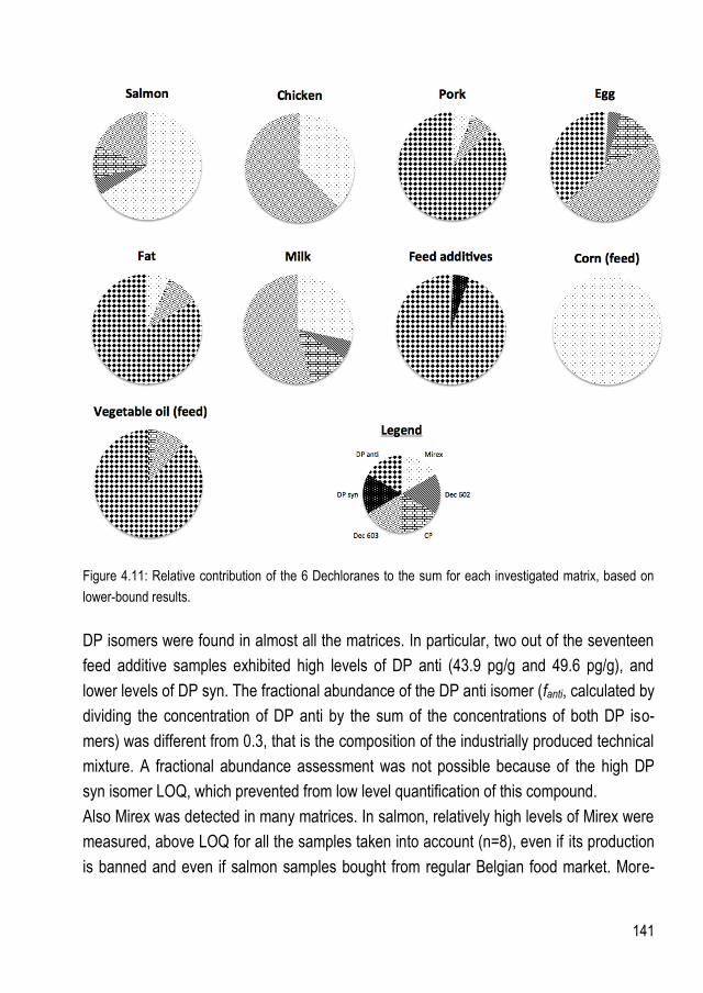
141
Figure 4.11: Relative contribution of the 6 Dechloranes to the sum for each investigated matrix, based on
lower-bound results.
DP isomers were found in almost all the matrices. In particular, two out of the seventeen
feed additive samples exhibited high levels of DP anti (43.9 pg/g and 49.6 pg/g), and
lower levels of DP syn. The fractional abundance of the DP anti isomer (fanti, calculated by
dividing the concentration of DP anti by the sum of the concentrations of both DP iso-
mers) was different from 0.3, that is the composition of the industrially produced technical
mixture. A fractional abundance assessment was not possible because of the high DP
syn isomer LOQ, which prevented from low level quantification of this compound.
Also Mirex was detected in many matrices. In salmon, relatively high levels of Mirex were
measured, above LOQ for all the samples taken into account (n=8), even if its production
is banned and even if salmon samples bought from regular Belgian food market. More-
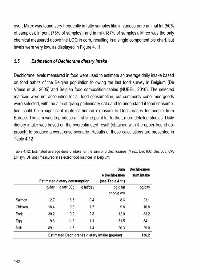
142
over, Mirex was found very frequently in fatty samples like in various pure animal fat (50%
of samples), in pork (75% of samples), and in milk (87% of samples). Mirex was the only
chemical measured above the LOQ in corn, resulting in a single component pie chart, but
levels were very low, as displayed in Figure 4.11.
5.5. Estimation of Dechlorane dietary intake
Dechlorane levels measured in food were used to estimate an average daily intake based
on food habits of the Belgian population following the last food survey in Belgium (De
Vriese et al., 2005) and Belgian food composition tables (NUBEL, 2010). The selected
matrices were not accounting for all food consumption, but commonly consumed goods
were selected, with the aim of giving preliminary data and to understand if food consump-
tion could be a significant route of human exposure to Dechloranes for people from
Europe. The aim was to produce a first time point for further, more detailed studies. Daily
dietary intake was based on the overestimated result (obtained with the upper-bound ap-
proach) to produce a worst-case scenario. Results of these calculations are presented in
Table 4.12
Table 4.12: Estimated average dietary intake for the sum of 6 Dechloranes (Mirex, Dec 602, Dec 603, CP,
DP syn, DP anti) measured in selected food matrices in Belgium.
Estimated dietary consumption
Sum
6 Dechloranes
(see Table 4.11)
Dechloranes
sum intake
g/day
g fat/100g
g fat/day
pg/g fat
or pg/g ww
pg/day
Salmon 2.7 16.5 0.4 8.6 23.1
Chicken 18.4 9.3 1.7 9.8 16.8
Pork 30.2 9.2 2.8 12.0 33.2
Egg 9.6 11.3 1.1 31.5 34.1
Milk 89.1 1.6 1.4 20.3 29.0
Estimated Dechloranes dietary intake (pg/day) 136.2

143
Reported levels suggested that Dechloranes enter the food chain and bioaccumulate,
hence humans are exposed via consumption of food, even if it is not possible to estimate
if food is the main route of exposure, as no data are available at the present for environ-
mental samples and environmental human exposure, considering the relevant levels pre-
viously reported in human blood. From what was seen at this stage, no class of foodstuff
can be highlighted as strongly contributing to human exposure to Dechloranes. More ex-
tensive and larger studies should be carried out to better understand fates of Dechloranes
and estimate other route of exposure, such as indoor dust.
6. Conclusions
A dedicated analytical method has been developed for the measurement of six members
of the Dechlorane family (Mirex, Dec 602, Dec 603, CP, DP syn, DP anti) in food and
feed. The use of ID and optimized PTV inlet parameters, as well as the use of GC-MS/MS
Triple Quad instrument, allowed trace level detection (ppb level) for all target compounds,
except Dec 604. The optimization steps focused on the improvement of the sensitivity,
from sample clean-up to sample injection and detection. 88 samples from 9 different ma-
trices, representing commonly consumed goods, were analyzed in order to preliminary
assess a daily intake of Dechloranes from food products. Levels in food and feed samples
were found to be close to the method limits of quantitation, except for some samples,
whose contamination appeared to be significantly higher. An estimation of the dietary in-
take showed that food was probably not the single route of exposure. Further studies are
necessary to understand contamination sources by Dechloranes and whether or not de-
tected levels could be harmful to human. Reported levels can be integrated in a global
study considering dust and other possible routes of exposure to investigate the contribute
of each source to human exposure. The analytical method developed for Dechlorane de-
tection at trace levels in food can be adapted, optimized and validated for Dechlorane
measurements in different matrices.
144
Bibliography
ATSDR, U. S. D. O. H. A. H. S. P. H. S.-A. F. T. S. A. D. R. 2000. TOXICOLOGICAL PROFILE FOR POLYCHLORINATED BIPHENYLS (PCBs).
BETTS, K. S. 2006. A new flame retardant in the air. Environmental Science and Technology, 40, 1090-1091.
BRASSEUR, C., PIRARD, C., SCHOLL, G., DE PAUW, E., VIEL, J. F., SHEN, L., REINER, E. J. & FOCANT, J. F. 2014. Levels of dechloranes and polybrominated diphenyl ethers (PBDEs) in human serum from France. Environment International, 65, 33-40.
CEQUIER, E., MARCÉ, R. M., BECHER, G. & THOMSEN, C. 2013. Determination of emerging halogenated flame retardants and polybrominated diphenyl ethers in serum by gas chromatography mass spectrometry. Journal of Chromatography A, 1310, 126-132.
DE VRIESE, S., DE BACKER, G., DE HENAUW, S., HUYBRECHTS, I., KORNITZER, K., LEVEQUE, A., MOREAU, M. & VAN OYEN, H. 2005. The Belgian food consumption survey: Aims, design and methods. Archives of Public Health, 63, 1-16.
FOCANT, J. F., EPPE, G., MASSART, A. C., SCHOLL, G., PIRARD, C. & DE PAUW, E. 2006. High-throughput biomonitoring of dioxins and polychlorinated biphenyls at the sub-picogram level in human serum. Journal of Chromatography A, 1130, 97-107.
FOCANT, J. F., EPPE, G., PIRARD, C. & DE PAUW, E. 2001. Fast clean-up for polychlorinated dibenzo-p-dioxins, dibenzofurans and coplanar polychlorinated biphenyls analysis of high-fat-content biological samples. Journal of Chromatography A, 925, 207-221.
FOCANT, J. F., PIRARD, C. & DE PAUW, E. 2004. Automated sample preparation-fractionation for the measurement of dioxins and related compounds in biological matrices: A review. Talanta, 63, 1101-1113.
GUERRA, P., FERNIE, K., JIMÉNEZ, B., PACEPAVICIUS, G., SHEN, L., REINER, E., ELJARRAT, E., BARCELÓ, D. & ALAEE, M. 2011. Dechlorane plus and related compounds in peregrine falcon (Falco peregrinus) Eggs from Canada and Spain. Environmental Science and Technology, 45, 1284-1290.
HOH, E., ZHU, L. & HITES, R. A. 2006. Dechlorane plus, a chlorinated flame retardant, in the Great Lakes. Environmental Science and Technology, 40, 1184-1189.
INCHEM, I. P. O. C. S. 1984. ENVIRONMENTAL HEALTH CRITERIA 44 [Online]. Available: http://www.inchem.org/documents/ehc/ehc/ehc44.htm.
JIA, H., SUN, Y., LIU, X., YANG, M., WANG, D., QI, H., SHEN, L., SVERKO, E., REINER, E. J. & LI, Y. F. 2011. Concentration and bioaccumulation of Dechlorane compounds in coastal environment of northern China. Environmental Science and Technology, 45, 2613-2618.

145
KAKIMOTO, K., NAGAYOSHI, H., TAKAGI, S., AKUTSU, K., KONISHI, Y., KAJIMURA, K., HAYAKAWA, K. & TORIBA, A. 2014. Inhalation and dietary exposure to Dechlorane Plus and polybrominated diphenyl ethers in Osaka, Japan. Ecotoxicology and Environmental Safety, 99, 69-73.
KEISR, K. L. E. 1978. The rise and fall of Mirex. Environmental science and Technology, 12, 8.
KIM, J., SON, M. H., KIM, J., SUH, J., KANG, Y. & CHANG, Y. S. 2014. Assessment of Dechlorane compounds in foodstuffs obtained from retail markets and estimates of dietary intake in Korean population. Journal of Hazardous Materials, 275, 19-25.
L'HOMME, B., SCHOLL, G., EPPE, G. & FOCANT, J. F. 2015. Validation of a gas chromatography-triple quadrupole mass spectrometry method for confirmatory analysis of dioxins and dioxin-like polychlorobiphenyls in feed following new EU Regulation 709/2014. Journal of Chromatography A, 1376, 149-158.
NUBEL 2010. Belgian food composition table, forth edition.: Ministry of Public Health, Brussels (Belgium).
PENG, H., WAN, Y., ZHANG, K., SUN, J. & HU, J. 2014. Trophic transfer of dechloranes in the marine food web of Liaodong bay, North China. Environmental Science and Technology, 48, 5458-5466.
PIRARD, C., FOCANT, J. F. & DE PAUW, E. 2002. An improved clean-up strategy for simultaneous analysis of polychlorinated dibenzo-p-dioxins (PCDD), polychlorinated dibenzofurans (PCDF), and polychlorinated biphenyls (PCB) in fatty food samples. Fresenius' Journal of Analytical Chemistry, 372, 373-381.
SHEN, L., REINER, E. J., MACPHERSON, K. A., KOLIC, T. M., SVERKO, E., HELM, P. A., BHAVSAR, S. P., BRINDLE, I. D. & MARVIN, C. H. 2010. Identification and screening analysis of halogenated norbornene flame retardants in the Laurentian Great Lakes: Dechloranes 602, 603, and 604. Environmental Science and Technology, 44, 760-766.
SÜHRING, R., FREESE, M., SCHNEIDER, M., SCHUBERT, S., POHLMANN, J. D., ALAEE, M., WOLSCHKE, H., HANEL, R., EBINGHAUS, R. & MAROHN, L. 2015. Maternal transfer of emerging brominated and chlorinated flame retardants in European eels. Science of the Total Environment, 530-531, 209-218.
SVERKO, E., TOMY, G. T., REINER, E. J., LI, Y. F., MCCARRY, B. E., ARNOT, J. A., LAW, R. J. & HITES, R. A. 2011. Dechlorane plus and related compounds in the environment: A review. Environmental Science and Technology, 45, 5088-5098.
WWW.POPS.INT/. Available: http://chm.pops.int/Convention/ThePOPs/ListingofPOPs/tabid/2509/Default.aspx.
ZHOU, S. N., SIDDIQUE, S., LAVOIE, L., TAKSER, L., ABDELOUAHAB, N. & ZHU, J. 2014. Hexachloronorbornene-based flame retardants in humans: Levels in maternal serum and milk. Environment International, 66, 11-17.
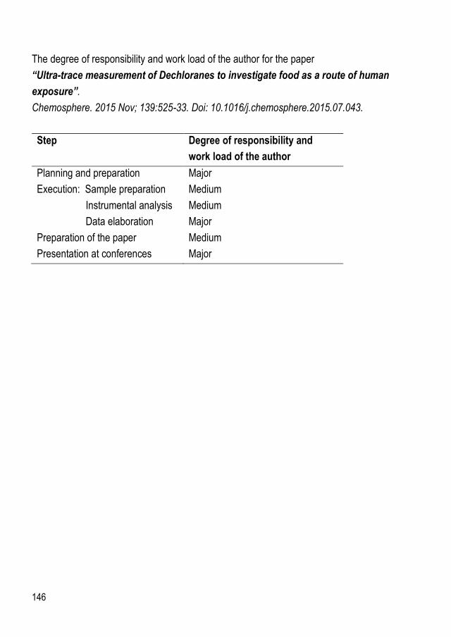
146
The degree of responsibility and work load of the author for the paper
“Ultra-trace measurement of Dechloranes to investigate food as a route of human
exposure”.
Chemosphere. 2015 Nov; 139:525-33. Doi: 10.1016/j.chemosphere.2015.07.043.
Step
Degree of responsibility and
work load of the author
Planning and preparation Major
Execution: Sample preparation
Instrumental analysis
Data elaboration
Medium
Medium
Major
Preparation of the paper Medium
Presentation at conferences Major
147
CONCLUSIONS
In this thesis analytical methods for POP detection in food and feed were developed and
validated. For instrumental quantification GC-MS/MS Triple Quad instrument was mainly
used, in addition to GC-HRMS Magnetic Sector. Part of the work of this thesis focused on
dioxins and PCBs, the other part was aimed to the quantification of emerging contami-
nants, Dechloranes.
In the dioxin and PCB framework, new high throughput clean-up approaches were devel-
oped and validated for dioxin and PCB detection in food and feed using automated sys-
tems. They demonstrated to be faster and more environmental and economically conven-
ient in comparison to existing procedures. Almost all the analyses were carried out with
GC-MS/MS Triple Quad instrument, as recently allowed from the EU Regulation in 2014.
For the DEXTechTM system, new approaches were based on 3 column set, namely multi-
layer silica, basic alumina, and a single carbon column, instead of classical 4 column set
using Florisil® and two carbon columns. Multilayer silica and two carbon columns were
commercially available, while alumina column was manually packed after proper thermal
treatment based on a modified EPA 1613 procedure. Two approaches arose from the
availability of two different carbon columns and led to different final fractionation profiles:
with Carbopack C:celite column, I-, MO- and co-PCBs were collected in fraction 1, and
PCDD/Fs were found infraction 2, with Norit:celite column, co-PCBs were found in frac-
tion 2 together with dioxins. Laboratories willing to use alumina columns can choose the
appropriate protocol based on the consecutive instrumental analysis. The new developed
approaches allowed time and solvent saving, respectively 27% and 18%, as well as
global cost reduction, giving recoveries in the range 60-120% as required by EU Regula-
tion.
“Alumina-Norit” method was applied to QC samples of pork fat, egg yolk and milk to as-
sess its performances on real fatty matrices and results showed that the clean-up method
was accurate, despite some issues related to manual packing. A full validation was not
carried out because of the high variability of the manual packing of alumina column. How-
ever, preliminary results of this work show that alumina columns can be used in the DEX-

148
TechTM system after slight modification of the system, because allow good quality sample
clean-up in accordance with EU Regulation. Alumina method can represent a valid alter-
native to the classic method based on Florisil®, allowing faster and cheaper sample clean-
up.
In Chapter 3 alternative clean-up approaches for PowerPrepTM system from FMS were
proposed, with the aim of having high throughput method for dioxin analysis with time,
solvent and global cost reduction. Alternative approaches were based on the validated
clean-up method used at the University of Liège and consisting of a preliminary lipid di-
gestion with a manually packed acidic silica column, followed by automated clean-up with
PowerPrepTM equipped with a 3 column setup: standard ABN silica, alumina, and carbon
column. “Short” and “fast standard methods” alternative approaches used the same col-
umn set and were suitable for low fat content samples (< 1 g) or they had to come after a
preliminary acidic digestion with manually packed acidic silica column to have fat capacity
of up to 7 g. They were designed from our routine automated method removing less cru-
cial steps, namely column washing/conditionings and tubing washing. Silica, alumina and
carbon column elution profiles were studied to assess minimum solvent amount for col-
umn elution. “Fast standard method” showed that also silica column initial conditioning
could be skipped without affecting final recoveries and extract quality. These new ap-
proaches allowed from 30 to 50% saving in terms of solvent and time.
Another method, referred to as “Jumbo” as based on four column set including a jumbo
acidic silica column, was developed as a fully automated alternative to our entire clean-up
procedure including the manual and the automated steps. Jumbo method used 4 column
set on the PowerPrepTM: high capacity acidic silica column, mini ABN silica, mini alumina
and carbon column, for a total fat capacity of up to 4 g and about 50% solvent and time
saving in comparison to our whole clean-up procedure. After development, the method
was tested on pork fat QC and vegetable oil to check the quality of the final extracts, and
it demonstrated to be suitable for trace level analysis of dioxins and PCBs. From these
preliminary tests it was also possible to understand that standard FMS alumina column is
oversized as mini alumina columns, containing the half of sorbent amount, showed to be
suitable for the scope.
Finally, a dedicated analytical method for the detection of Dechlorane compounds (six
members of the Dechlorane family: Mirex, Dec 602, Dec 603, CP, DP syn, DP anti) was
149
presented. The use of ID and optimized PTV inlet parameters, as well as the use of GC-
MS/MS Triple Quad instrument, enabled trace level detection (ppb level) for all target
compounds. Some instrumental parameters for PTV inlet were set by means of the Ex-
perimental Design. The method was validated according to the applicable criteria reported
in the EU Regulation for dioxin analysis and was applied to 88 samples from 9 different
matrices, representing commonly consumed goods, with the idea of assessing daily die-
tary intake of Dechloranes. Levels in food and feed samples were found to be close to the
method limits of quantitation, except for some samples, whose contamination appeared to
be significantly higher. An estimation of the dietary intake showed that food was probably
not the unique route of exposure. Further studies are necessary to understand contami-
nation sources by Dechloranes and whether or not detected levels could be harmful to
human. Reported levels can be integrated in a global study considering dust and other
possible routes of exposure to investigate the contribute of each source to human expo-
sure. The analytical method developed for Dechlorane detection at trace levels in food
can be adapted, optimized and validated for Dechlorane measurements in different matri-
ces.

150

151
ACKNOWLEDGEMENTS
This PhD has been an amazing experience of work and life. During these years of work I
have been learning so many things from the scientific point of view, but also from the per-
sonal one, as I moved to Belgium with a big change in my personal life.
Thanks to my supervisors, Prof. Jean François Focant (University of Liège), Prof. Carlo
Zambonin (University of Bari), Dr. Cosima Damiana Calvano (University of Bari) and Prof.
Pietro Mastrorilli (Polytechnic Univeristy of Bari) for making this PhD possible and for the
cooperation among the Institutions. Thanks to Prof. Michele Mossa and Prof. Antonio
Felice Petrillo, the coordinators of my Doctoral School in the Polytechnic University of Bari
for their precious advices and guidelines. Thanks to all of them for their scientific and hu-
man support. Thanks to Prof. Jean François Focant for welcoming me in his lab and for
treating me like one of his students since the first day in 2014. It is also because of this
that the initial short collaboration ended up in a PhD in joint agreement. Thank you for all
the opportunities you have given to me, for all you taught me in the lab and outside the
lab. Thanks for making it possible for me to attend several conferences, to build my scien-
tific network and for the research stays abroad. Thanks for the respect you have always
given to me, and for the freedom of personal and scientific expression.
Thanks to my colleague Benjamin L’Homme from the University of Liège for sharing with
me and for transferring me his knowledge and expertise. Thanks to the people in CART
laboratory (University of Liège): Georges Scholl for the interpretation of final results and
the continuous scientific support, Cedric Van Aefferden and Nathalie Didderen for teach-
ing me the sample preparation in dioxin analyses, and Angelique Leroy for the interpreta-
tion of the results. I have been lucky to carry out my PhD in such environment, as I have
been able to gain high level expertise.
Thanks to my thesis referees, Prof. Gauthier Eppe (University of Liège), and Dirk
Krumwiede (Thermofisher) for reading and improving the present thesis.
I would like to acknowledge the funding of my PhD scholarship, with special mention for
the Interpolytechnic School and the Lerici Foundation. Thanks to FMS, LCTech and Ag-
ilent for the instrumental support and for the interest in my research activity.

152
And last but not least, thanks to my family for the great support for everything in my life, in
the past, at the present and in the future. You are my strength.
Thank you Jérémy for putting up with me, especially when changing the plans, the
schedule and the holidays. Your moral support has been essential for my serenity and the
success of this work. Thanks for being my family in Belgium.
I am proud of myself because of all the goals reached in this PhD and all the steps for-
ward done in these years, despite the adverse situations. Et je suis fière de moi aussi
parce que j’ai appris à parler et à écrire en Français finalement!

153
CURRICULUM
Personal details
Name and family name: Chiara Calaprice
Date and place of birth: 04/03/1983
Permanent address:
via Giacomo Matteotti 16, 70010 Adelfia (Bari) - Italy
Current address:
rue du Chataigner 9, 4100 Boncelles Seraing (Liege) - Belgium
Correspondence address:
Allèe du 6 Aout, 11 Bat. B6c-local R1, 4000 Liege - Belgium
Email: [email protected]
Phone number: +32 477 586 770
+39 328 42 19 573
Education
PhD in analytical chemistry in persistent organic pollutants (POPs) field
2013 – 4th April 2016 Polytechnic University of Bari and Interpolytechnic School (Italy) and University
of Liège (Belgium)
- Joint PhD in Environmental and Territory Safety and Control - Analytical
Chemistry
2010 - 2011 University of Easter Piedmont, Alessandria (Italy)
Master graduation in Chemistry
2009 University of Easter Piedmont, Novara (Italy)
Post-graduation specialization course on materials for energy and environment
2002 - 2008 University of Bari (Italy)
Bachelor degree in Chemistry
154
Research expertise
- Development of new sample clean-up techniques in dioxin analysis using automated systems
(PowerPrepTM from FMS Inc., DEXTechTM from LCTech Gmbl)
- GC-MS/MS Triple Quad advanced user (Agilent)
- Development and validation of analytical methods for Persistent Organic Pollutants (POPs) detection in
food and feed matrices with GC-MS/MS Triple Quadrupole instruments (Agilent)
- Multivariate analysis (PCA, cluster analysis) and modelling (MLR, PLS) with Matlab, Statistica and the Un-
scrambler
- Experimental design (DoE)
- LC-MS/MS, LC-MS
- Development and validation of analytical procedures for pesticides detection in food matrices
Research stays
Feb 2014 - ongoing University of Liège (Belgium) – joint agreement with Polytechnic University of
Bari for the research in POP and dioxin analysis.
2nd - 22nd Dec 2015 Orebro University (Sweden) – sample preparation for low volume samples of blood. Supervisors: Dr. Ingrid Erickson and Prof. Bert Van Bavel
Feb – May 2011 Internship for master thesis: Eni Taranto Refinery (Italy)
- Chemometrics, multivariate analysis for process optimization
Jul – Nov 2009 Internship for post-graduation course: Donegani Institute, Research Centre for Non-
Conventional Energy of Eni S.p.A (Italy)
- Organic synthesis, heterogeneous catalysis
Total list of publications
1 “Optimization of a new dioxin/PCB clean-up and fractionation procedure for an existing automated
system”.

155
Calaprice C., Calvano C.D., Zambonin C., Focant J.-F., Organohalogen Compounds, Vol 77 (2015),
733-735
2 “Ultra-trace measurement of Dechloranes to investigate food as a route of human exposure”
L’Homme B., Calaprice C., Calvano C. D., Zambonin C., Leardi R., Focant J.-F. ; Chemosphere, 139
(2015), 525–533
3 “Measurement of trace level Dechlorane flame retardants in food and feed by GC-MS/MS”
L’Homme B., Calaprice C., Brasseur C., Calvano C.D., Zambonin C., Leardi R., Focant J.-F.; Or-
ganohalogen Compounds, Vol 76 (2016), 1460-1463
4 “Co-production of butyrate methyl ester and triacetylglycerol from tributyrin and methyl acetate”
Battistel E., Calaprice C., Gualdi, E., Rebesco, E., Usai, E.M., Applied Catalysis A: General, 394
(2011), 149–157
Conferences
Oral presentations
1 “Fatty Matrices Cleaned-up with a Different Approach”,
Invited speaker at “1st DEXTech™ User Meeting” – 21st and 22nd October at Governmental Lab Chemical and Veterinary Investigation Office (CVUA-MEL)- Muenster (Germany)
2 “Optimization of a new dioxin/PCB clean-up and fractionation procedure for an existing automated system”
At the 35th International Symposium on Halogenated Persistent Organic Pollutants – Dioxins 2015”, 23rd – 28th August 2015 in Sao Paulo (Brasil).
3 “Ultra-trace measurement of Dechloranes to investigate food as a route of human exposure” (Otto Hutzinger award)
At the 35th International Symposium on Halogenated Persistent Organic Pollutants – Dioxins 2015”, 23rd – 28th August 2015 in Sao Paulo (Brasil).
4 “Ultra-trace measurement of Dechloranes in food and feed”
At Massa 2015, conference on mass spectrometry by the mass spectrometry division of the Italian Chemical Society, 10th – 13th June 2015 in Alghero (Italy),
5 “Measurement of ultra-trace levels of Dechloranes in food and feed. Assessment of dietary intake”
At the 10th International Symposium on Recent Developments in POPs Analysis, organized by

156
Thermo Fischer on 29th and 30th April 2015 in Prague (Czech Republic)
6 “Measurement of trace level Dechlorane flame retardants in food and feed by GC-MS/MS”
At the 34th International Symposium on Halogenated Persistent Organic Pollutants – Dioxins 2014, 31st – 5th September 2014, Madrid (Spain)
Poster presentation
1 “Revisiting an existing dioxin/PCB clean-up and fractionation procedure to reduce solvent and time consumption”
At the 35th International Symposium on Halogenated Persistent Organic Pollutants – Dioxins 2015”, 23rd – 28th August 2015 in Sao Paulo (Brasil).
2 “Study of the effects of heating on quality of soymilk proteins by means of MALDI-TOF MS”
At the “4th MS-J-Day - I giovani e la spettrometria di massa”, 4th November 2013, Potenza (Italy)
Awards and scholarship
2015 Otto Hutzinger award: for outstanding student presentations at the annual Dioxin Symposium to
acknowledge their scientific contribution to the field of halogenated persistent organic pollutants
(http://www.dioxin20xx.org/award_winners.htm)
2015 Lerici scholarship: for Italian PhD student to carry out a research project in Sweden (research
stay in December 2015)
2014 Scuola Interpolitecnica di Dottorato: additional grant for selected PhD students from the 3 Italian
Polytechnic Universities Turin- Milan - Bari
2013 Fondo Giovani: 3 years grant for PhD students from the Italian Minister of University and Re-
search.
2009 Ritorno al futuro: European scholarship for people from Puglia (Italy) to attend post-graduation
courses in scientific field
Working and practical experience
Feb - Sept 2012 Laboratory technician at BonassisaLab s.r.l, Foggia (Italy) (www.bonassisa.it)

157
- LC-MS/MS detection of mycotoxins and pesticides in food
- Nutrition facts determination
- GC-FID detection of fatty acids in food matrices
Languages
Native language Italian
B2 (certified) English
B1 French
References
Prof. Jean François Focant University of Liège (Belgium) [email protected] +32 (0)4 366 35 31