August 13, 2004 1

POLYMER MODELING IN INDUSTRY

Jozef Bicerano, Ph.D.Bicerano & Associates, LLC

For further details on most of the work summarized in these slides, see J. Bicerano, S. Balijepalli, A. Doufas, V. Ginzburg,J. Moore, M. Somasi, S. Somasi, J. Storer and T. Verbrugge,

“Polymer Modeling at The Dow Chemical Company”, J. Macromol. Sci.-Polymer Reviews, 44, 53-85, 2004.

August 13, 2004 2

INTEGRATED MODELING APPROACH

New product and/or process development in industry requires attention to many (and often contradictory) considerations: Formulation design. Raw material costs. Processing costs. Product performance targets. Market trends. Governmental regulations.

A multidisciplinary and integrated modeling approach is desirable since the relevant materials science encompasses many phenomena.

August 13, 2004 3

Multidisciplinary Nature of Industrial ModelingPr

oble

m D

efin

ition

The

Goa

l

NumericalModeling

Model Formation

User Interface &Tools

Problem DefinitionCustomer Requirements

CPUNumerical Methods

Software Code

First PrinciplesPhenomenology

Empiricism

DeterministicStochastic

August 13, 2004 4

“Holy Grail”: Multiscale Modeling Paradigm

Chemical structures of system components (polymers, molecular fluids, surfactants, fillers, etc.)

Modeling at molecular scale (QSPR, atomistic simulations)

Binary interaction parameters (Flory-Huggins or its analogues) between all distinct pairs of system components

Modeling at mesoscale (self-consistent mean field theory for thermodynamic equilibrium; mesoscale dynamic

simulations for evolution as a function of time)

Phase diagrams, interfacial tensions, phase inversion points, model-generated three-dimensional snapshots of morphology as a function of time and of thermodynamic equilibrium morphology

Modeling at the macroscale (computational fluid dynamics, solid mechanics)

Understanding and predictions of bulk sample behavior (morphological stability, flow characteristics, physical

and mechanical properties)

August 13, 2004 5

BRIEF REVIEWS OF SELECTED PROJECTS

Mechanical properties of thermoplastics (Jonathan Moore).

Polymer/clay nanocomposites (Valeriy Ginzburg).

Polyol templating (Sudhakar Balijepalli).

Flow-induced crystallization and polymer process modeling (Antonios Doufas and Madan Somasi).

High-throughput polymer design (Sweta Somasi and Jozef Bicerano).

Controlled release of drugs from hydrophilic polymers (Sweta Somasi, Irina Graf, Steve Ceplecha, Daniel Simmons and Jozef Bicerano).

Branched/network polymer structures (Tom Verbrugge).

Water vapor transport in a polymer matrix composite (Joey Storer, Jozef Bicerano and Dave Moll).

August 13, 2004 6

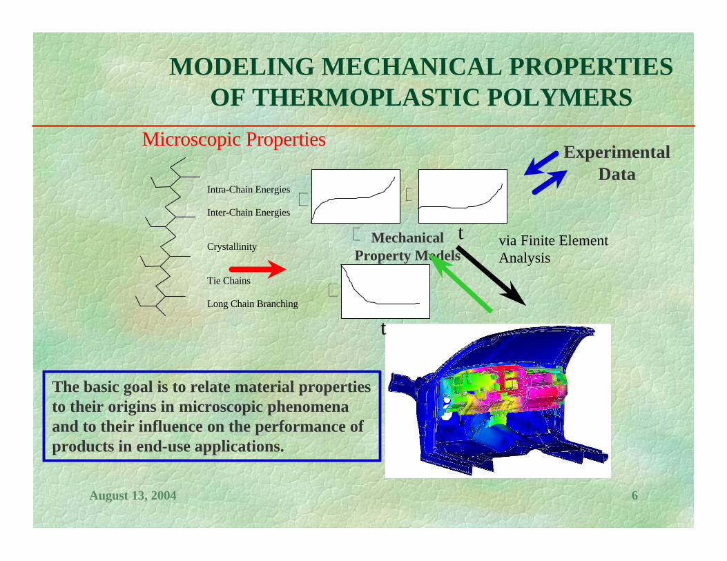
MODELING MECHANICAL PROPERTIESOF THERMOPLASTIC POLYMERS

The basic goal is to relate material properties to their origins in microscopic phenomenaand to their influence on the performance of products in end-use applications.

Mechanical Property Models

Experimental Data

Intra-Chain Energies

Inter-Chain Energies

Crystallinity

Tie Chains

Long Chain Branching

t

t via Finite ElementAnalysis

Microscopic Properties

August 13, 2004 7

Physical Picture for Glassy Thermoplastic Polymers

A mosaic of nanoscale clusters: Distribution of differing cluster

viscoelastic characteristics. Fluctuations of the Eyring-type

activation energy for yielding induce dynamic inhomogeneities.

“Locally yielded” regions that no longer respond elastically (solid black clusters) become more abundant with increasing strain.

August 13, 2004 8

Distribution of Yield Characteristics Related to d/d

233 < T (K) < 338

1.6x10-3 < strain rate (sec-1)

< 1.6x10-1

Bisphenol-A polycarbonate

MFR ~ 10

August 13, 2004 9

Strain Rate and Temperature Dependences

Dashed lines are calculated.Solid lines are experimental data.

August 13, 2004 10

Thermoplastic Mechanical Property Modeling Summary

The model requires three stress-strain curves as input for calibration.

It captures the stress-strain curves up to yield accurately at different rates and temperatures for bisphenol-A polycarbonate.

Limited testing suggests that it works well for other glassy polymers, such as ABS, PC/ABS, and HIPS.

It also provides insights into the fundamental issue of glass-former "fragility" in the glassy state and a practical means to assess dynamic inhomogeneities in polymeric glasses.

For further details, see J. Moore, M. Mazor, S. Mudrich, J. Bicerano, A. Patashinski and M. Ratner, ANTEC ’02 Preprints, Society of Plastics Engineers, 1961-1965 (2002).

August 13, 2004 11

MULTISCALE MODELING OFPOLYMER/CLAY NANOCOMPOSITES

SCFT

Clay (chemical structure),organic modifier (chemical structure, amount, MW),polymer (structure, MW)

Effective clay-clay interactions

Clay aspect ratio,organoclay loading

DFT

WAXS and SAXS

TEM

Phase behavior, morphology

PALMYRAMechanical Properties(Young’s Modulus)

Physical Properties(Thermal

Conductivity)

August 13, 2004 12

Dispersing Unmodified (Virgin) Clay in Polymer:• Calculate polymer-induced clay-clay interactions:

Entropy -- polymer pushed outEnthalpy -- polymer pulled in

• Enthalpy needs to dominate• Best way -- use polar head group

(such as MaPP for PP/clay hybrids)

For Success With Organically Modified Clays:• Organic modifier chains should be sufficiently long.• Organic modifier and polymer should be miscible.• Polymer should be attracted to clay surface.

Vaia and Giannelis, Macromolecules, 30, 7990-7999 (1997).

Immiscible

Intercalated

Exfoliated[E

nerg

y/un

it a

rea]

Distance, nm

Modeling Clay Intercalation or Exfoliation:Mean-Field Theory of Polymers in the Galleries

August 13, 2004 13

Modeling Clay Dispersion Morphology

Clay surface coverage and organoclay loading determine the equilibrium morphology, but in practice the morphology is often non-equilibrium.

Morphology can be deduced experimentally from WAXS, SAXS and TEM.

Immiscible

Exfoliated

Clay-Clay Potentials (SCMFT)

Increase inEnd-FunctionalizedPolymer AdsorptionEnthalpy (units: kT)Onto Clay Surface

Ginzburg and Balazs, Adv. Mater., 12, 1805-1809 (2000).

Organoclay Loading

Two-Phase (Part. Exf., Part. Stacks)

Isotropic Exf.

Aligned Exf.

Aligned Int.

Clay StacksIso. Gel

Dispersion Phase Behavior (DFT)

August 13, 2004 14

Verifying Dispersion Morphology Using WAXS

XRD fitting model can determine degree of exfoliation in clay dispersions. Results in qualitative agreement with transmission electron micrographs.

XRD Intensity

0

5000

10000

15000

20000

25000

30000

0 2 4 6 8

2 Theta, degI,

arb.

uni

ts

ExperCalc

System 2: ~50% single layers, the rest in stacks of 6-8 platelets each with interlayer separation ~ 3.9 nm

XRD Intensity

0

10000

20000

30000

40000

50000

60000

70000

80000

0 2 4 6 8

2 T h e ta , d e g

I, ar

b. u

nit

s

E xpe rC a lc

System 1: <10% single layers, the rest in stacks of 20-30 platelets each with interlayer separation ~ 3.7 nm

Calculations based on a model by Vaia and Liu, Polymeric Materials: Science & Engineering, 85, 14-15 (2001).

August 13, 2004 15

Predicting Mechanical Properties of Nanocomposites Using Finite Element Models

Young’s modulus depends strongly on extents of platelet exfoliation and alignment. Similar methods are applicable to predicting other properties.

• For randomly oriented disks, no significant dependence of

Young’s modulus on exfoliation.

• For aligned disks, in-plane modulus improves with increased exfoliation.

See also: D. A. Brune and J. Bicerano, Polymer, 43, 369-387 (2002), whereclosed-form equations were used tomodel more idealized morphologies.1.0

1.1

1.2

1.3

1.4

1.5

1.6

1.7

1.8

1.9

2.0

0.0 0.5 1.0 1.5 2.0 2.5 3.0 3.5 4.0 4.5 5.0Clay Loading, Weight %

E(co

mpo

site

) / E

(mat

rix)

No Stacks, Aligned, In-plane50%Stacks, Aligned, In-plane100%Stacks, Aligned, In-planeNo Stacks, Random50% Stacks, Random100% Stacks, Random

August 13, 2004 16

Nanocomposite Modeling Summary

Implemented multiscale modeling framework relating properties of nanocomposites to their formulations: Polymer/Clay Miscibility -- Mean-Field Theory of Polymers. Phase Behavior of Dispersions -- DFT of Colloids. Morphology Verification -- XRD Analysis and Modeling. Property Prediction -- Finite Element Analysis.

Modeling framework was applied successfully to: Design compatibilizer formulations to improve clay dispersion

in aqueous and other solutions, as well as in polymer melts. Estimate mechanical properties of specific nanocomposites.

August 13, 2004 17

POLYOL TEMPLATING

Predict phase diagram, including transitions.

Many applications in nanotechnology.

August 13, 2004 18

Assumptions in Lattice Mean-Field Model(developed by Per Linse et al., Lund University)

Space divided into equal-sized lattice sites in two dimensions.

One species per lattice site.

Flexible polymers.

Mean-field approximation, with nearest neighbor interactions accounted for via Flory-Huggins interaction () parameters.

Aqueous solutions of PEO and PPO homopolymers display a lower critical solution temperature.

EO and PO segments are each modeled in terms of “polar” and “apolar” internal states.

August 13, 2004 19

0 0.2 0.4 0.6 0.8 1

280

300

320

340

360

polymer

T [K

]

H1

L

L

I1

H2

I2

Ordered Phases: Disordered Phase: LMicellar cubic: I1Hexagonal: H1Lamellar: LReverse hexagonal: H2Reverse micellar cubic: I2

Main Features of Phase Diagram for an AB-EO Triblock / Water System

Lyotropic Phase Transitions:Caused by concentration changes (for example, H1 L

as polymer is increased).

Thermotropic Phase Transitions:Caused by temperature changes (for example, H1 L I2 as T is increased).

August 13, 2004 20

hydrophobic hydrophilic

Intermediate temperature

hydrophobic hydrophilic

High temperaturehydrophobic hydrophilic

Low temperature

Thermotropic Behavior From Increasing Effective Hydrophobicity With Temperature

Water-continuous phases with high curvature dominate.

Lamellar phase is narrow. No stable “reverse” (polymer-

continuous) phase is found.

Lamellar phase is stable.

“Reverse” (polymer-continuous) phases become more stable.

August 13, 2004 21

Block Length Effects on Thermotropic Transitions

Increasing the EO block length extends the temperaturestability of ordered phases and favorswater-continuous phases.

0 0.2 0.4 0.6 0.8 1

280

300

320

340

360

polymer

T [K

] H1

L

L

I1

(CH2)14-PO12 -EO34

0 0.2 0.4 0.6 0.8 1

280

300

320

340

360

polymer

T [K

]

L

I2 H

2

H1

L

(CH2)14-PO12-EO8

0 0.2 0.4 0.6 0.8 1

280

300

320

340

360

polymer

T [K

]

H1

L

L

I1

H2

I2

(CH2)14-PO12 -EO17

280

300

320

340

360 H1

L

T (K

)

0 0.2 0.4 0.6 0.8 1

polymer

(CH2)14-PO12 -EO68

August 13, 2004 22

Polyol Templating Summary

Lattice mean-field theory was used to predict the lyotropic and thermotropic phase transitions of polyol surfactants with water, as functions of chemical composition, block length and concentration.

This work is discussed in greater detail in several publications: N. P. Shusharina, S. Balijepalli, H. J. M. Grünbauer and P. Alexandridis,

ACS Polymer Preprints, 43(2), 354-355 (2002). N. P. Shusharina, P. Alexandridis, P. Linse, S. Balijepalli and H. J. M.

Grünbauer, Eur. Phys. Jour. E, 10, 45-54 (2003). N. P. Shusharina, S. Balijepalli, H. J. M. Grünbauer and P. Alexandridis,

Langmuir, 19, 4483-4492 (2003). P. Alexandridis, N. P. Shusharina, K.-T. Yong, K.-K. Chain, S. Balijepalli

and H. J. M. Grünbauer, ACS Polymer Preprints, 44(2), 218-219 (2003).

August 13, 2004 23

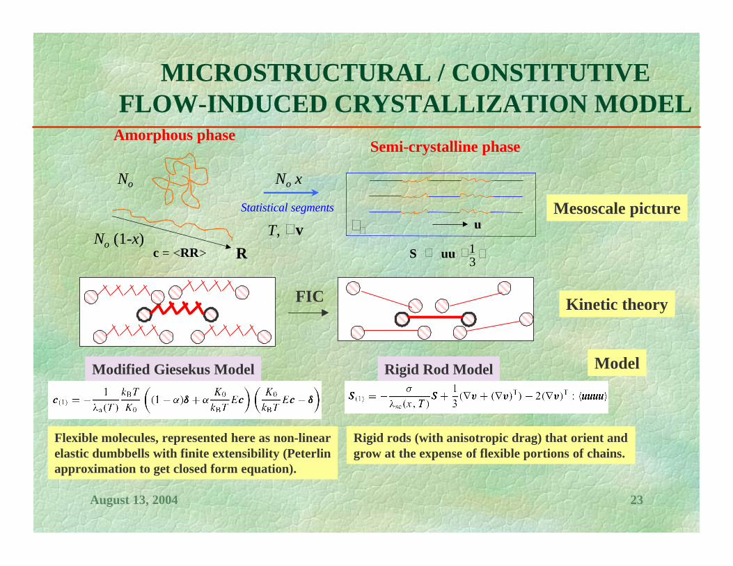
MICROSTRUCTURAL / CONSTITUTIVEFLOW-INDUCED CRYSTALLIZATION MODEL

Rc = <RR>

Amorphous phaseSemi-crystalline phase

No x

u

δ31 uuS

Statistical segments

No (1-x) T, v

No

FIC

Mesoscale picture

Kinetic theory

Modified Giesekus Model Rigid Rod Model

Rigid rods (with anisotropic drag) that orient and grow at the expense of flexible portions of chains.

Flexible molecules, represented here as non-linearelastic dumbbells with finite extensibility (Peterlin approximation to get closed form equation).

Model

August 13, 2004 24

Modeling Fiber Spinning and Film Blowing Processes

Spinneret

Take-up roll

Mass throughput W

rzz = 0vz = voD = DoT = To

z = Lvz = vLD = DL

Lvc, Ta

z1

z2

Quench air

Freeze point

Air

Flattened Tube

P

1

2z

r

L

Cooling AirH(z)

R(z)

RL

Nip rolls

z

Fiber Spinning Film Blowing

Must solve the coupledmass, momentum and

energy conservation andconstitutive/crystallization

equations numerically.Frost line

August 13, 2004 25

Fiber Spinning Model Validation

Distance from Spinneret [cm]0 20 40 60 80 100 120 140 160

Axi

al V

eloc

ity [m

/min

]

0

1000

2000

3000

4000

5000

6000

Bir

efri

ngen

ce

0.00

0.01

0.02

0.03

0.04

velocity

birefringence

Distance from Spinneret [cm]0 40 80 120 160

Dia

met

er, T

empe

ratu

re

0.1

1

10

100

Bire

frin

genc

e

0

20

40

60

80

100

vzn

n x 103

T x 0.1 oC

D

5100 m/min

5947 m/minNYLON 6,6PET

The model predictions are in good agreement with high-speed spinning data for the velocity, diameter (necking), temperature, and flow birefringence of Nylon and PET.

August 13, 2004 26

Linear Stability Analysis for Fiber Spinning

Eigenspectrum for two different take-up speeds

Stress disturbance evolution at end of spinline at most dominant eigenvaluefor the two take-up speeds

-12

-8

-4

0

4

0 100 200 300 400

R

Stable (Draw Ratio=50)

Unstable (Draw Ratio=100)

-20

-10

0

10

20

0 0.5 1 1.5 2Time

Stre

ss

DrawRatio=50

Draw Ratio=100

To predict the onset and evolution of instabilities (draw resonance), the system of equations is linearized around the steady state and the time evolution of prescribed disturbances is monitored. This evolution is dictated by the eigenvalues of the system.

August 13, 2004 27

Blown Film Model Validation

Distance from Die [m]0 1 2 3 4 5

Axia

l Vel

ocity

[m/s

]

0.0

0.2

0.4

0.6

0.8

1.0

data, run 56model, run 56data, run 57model, run 57data, run 50model, run 50

(1)

(2)

(3)

Distance from Die [m]

0.0 0.2 0.4 0.6 0.8 1.0

Tem

pera

ture

[o C]

20

40

60

80

100

120

140

160

data, run 50data, run 56data, run 57model, run 50model, run 56model, run 57

Prediction of bubble velocity and temperature profiles

The model can predict film velocity and temperature profiles accurately and capture the plateau of the film temperature due to crystallization.

August 13, 2004 28

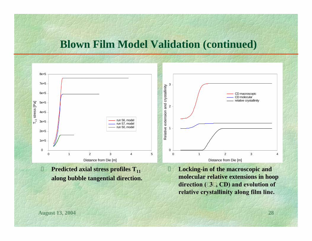
Blown Film Model Validation (continued)

Distance from Die [m]

0 1 2 3 4 5

T 11 s

tress

[Pa]

0

1e+5

2e+5

3e+5

4e+5

5e+5

6e+5

7e+5

8e+5

run 56, modelrun 57, modelrun 50, model

Distance from Die [m]

0 1 2 3 4

Rel

ativ

e ex

tens

ion

and

crys

talli

nity

0

1

2

3

CD macroscopicCD molecularrelative crystallinity

Predicted axial stress profiles T11

along bubble tangential direction. Locking-in of the macroscopic and

molecular relative extensions in hoop direction (“3”, CD) and evolution of relative crystallinity along film line.

August 13, 2004 29

Flow-Induced Crystallization Modeling Summary

Model is mesoscopically-based, applicable to a variety of kinematics (uniaxial or biaxial extension, shear), and able to simulate polymer processes of great industrial and academic interest quantitatively.

Predicts necking and the associated softening (decrease of the extensional viscosity at high draw ratios) behavior in fiber spinning for the first time.

Predicts stresses in and microstructures of fibers and films at the freeze point, which are closely related to the mechanical and physical properties.

Predicts effects of fabrication conditions and molecular architecture on draw resonance during non-isothermal fiber spinning.

Predicts rheometric data (such as Meissner, Rheotens, shear) in absence of crystallization.

See the many publications of Doufas et al. for further details.

August 13, 2004 30

HIGH-THROUGHPUT POLYMER DESIGN

The approach attempted at Dow was based on J. Bicerano, Prediction of Polymer Properties, third edition, Marcel Dekker, New York (2002), as implemented in the SYNTHIA software module marketed by Accelrys, Inc.

Researcher guesses some candidate repeat units that may perhaps give polymers satisfying performance criteria for target application.

Properties are predicted to select the best candidates for synthesis, which are limited to being just a subset of the researcher’s initial guesses.

Conventional “Forward Engineering” Approach

High-throughput (combinatorial) methods are used to generate a vast “library” of repeat unit structures, and properties are predicted for the polymers of these repeat units.

The best candidates for synthesis are identified from this huge repeat unit library, possibly providing attractive candidates that the researcher would never have thought of.

More Powerful “Reverse Engineering” Approach

August 13, 2004 31

CERIUS2/SYNTHIA Approach

Enter all repeat units and property predictions by using SYNTHIA once into a database

Dow software enumerating all possible repeat unit structures that can be builtcontaining up to a certain number of the subunits from a “fragment library”

Generate fully extended and optimized repeat unit geometries by using Dow softwarefor conformational search in combination with CERIUS2 for energy minimization

Search databaseSelection Criteria Selected Candidates

Generate initial repeat unit structures using CERIUS2

August 13, 2004 32

High-Throughput Polymer Design Summary

Enumeration Program Builds repeat units for CERIUS2Backbone Program Changes torsion angles to 180o or 0o

and stores all such conformationsCERIUS2 Minimizes energies of conformationsCompare Program Compares conformations, finds one

with maximum extension, saves itSYNTHIA Predicts properties at T= 200K to 500K

for stored conformations, saves outputin database-compatible XML format

Database Stores conformations and predictions in a readily searchable format (work not completed on this component of system)

SYNTHIA was endowed with combinatorial modeling capabilities!

August 13, 2004 33

High-Throughput Polymer Design: Work in Progress

Bicerano & Associates, LLC, is working with DTW Associates, Inc., to develop a much more effective new modeling approach to high-throughput polymer design.

This approach will be implemented as a new module (HTPD) which will be made commercially available in DTW’s Polymer-Design Tools™ suite of software tools.

August 13, 2004 34

CONTROLLED RELEASE OF DRUGSFROM HYDROPHILIC POLYMERS

DrugFiller

Water

HPMC

Dissolutionof polymer

Diffusion of water, drug and filler

Swelling of tabletand formation of gel

• Diffusion of water into tablet.• Diffusion of drug/filler out of tablet.• Dissolution of polymer matrix.• Swelling of tablet as water enters.• Formation of gel.

Simultaneous Processes:

August 13, 2004 35

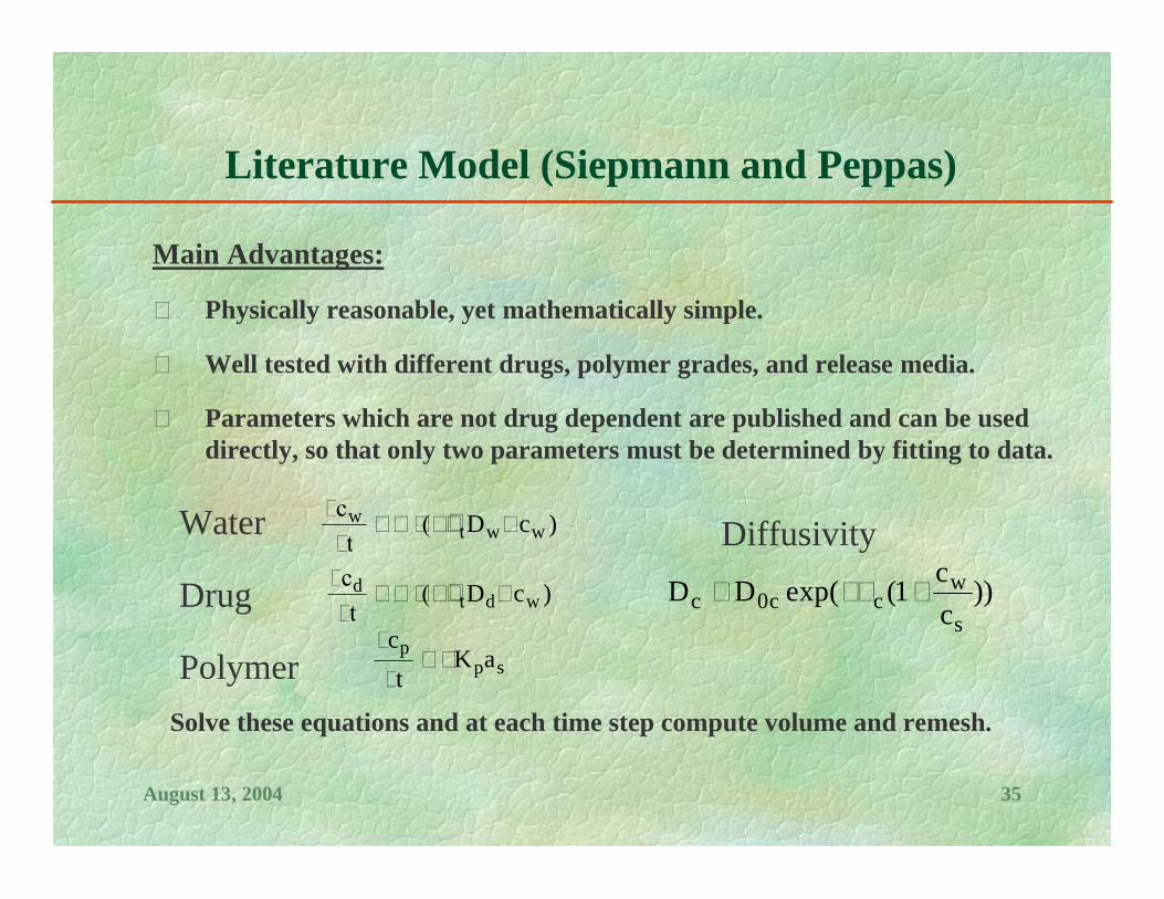
Literature Model (Siepmann and Peppas)

Main Advantages:

• Physically reasonable, yet mathematically simple.

• Well tested with different drugs, polymer grades, and release media.

• Parameters which are not drug dependent are published and can be used directly, so that only two parameters must be determined by fitting to data.

)cDˆ(t

cwwt

w

)cDˆ(t

cwdt

d

spp aKt

c

Water

Drug

PolymerSolve these equations and at each time step compute volume and remesh.

))cc1(exp(DD

s

wcc0c

Diffusivity

August 13, 2004 36

User Interface

Graphical representationof experimental

results and model predictions

Interface to choose input

parameters (tablet size, loading, etc.)

Interface to either input

values for modelparameters or choose them to

be fitted by using a state-of-the-art particle

swarm optimizer

Standard deviation – to determine goodness of fit.

Can export results to Excel & many other features!

August 13, 2004 37

Results With Siepmann-Peppas Model

Fitted controlled release data for six different drugs of same family (water-solublebronchodilators) from a literature reference, from a hydroxypropylmethylcellulose matrix (50% drug loading by weight), by using the Siepmann-Peppas model.

The drug diffusivity shows dependence on “cavity surface area” (also known as the “solvent-accessible surface area”) of the drug molecules.

0.E+005.E-071.E-062.E-062.E-06

3.E-063.E-064.E-064.E-065.E-06

3 4 5 6 7

Cavity Sirface Area (nm2)

Dru

g D

iffus

ivity

(cm

2/s)

PhenylpropanolamineEphedrine

Salbutamol

TerbutalineAminophylline

Reproterol

0

20

40

60

80

100

0 2 4 6 8time, h

drug

rele

ased

, %

August 13, 2004 38

MODELING BRANCHED/NETWORK POLYMERS

This work is aimed towards understanding the following relations:

One can then predict industrially important parameters (such as the time to gel, critical gel ratio, polymer molecular weight and viscosity buildup).

One can also gain insights on aspects of branched and/or network architectures where analytical tools fail (such as the compositions and sequence distributions of the elastic chain segments between crosslinks, dangling ends, loops).

Most importantly, success in this effort can shorten the product development time by providing models to guide the experimental work.

reactant structuresnetwork structure

reaction conditionsnetwork

properties

August 13, 2004 39

Miller-Macosko– Recursive Approach– Extended Capabilities– ST = sec (DWS)

– Diffusion and Kinetic Controlled– Most realistic representation– ST = hour (SGI)

3D-Percolation

ARS & Rate Theory– Flory-Stockmayer– Limited Capabilities– ST = min (SGI)

– Off-space percolation– Allows 1st and 2nd kinetics– ST = min - hour (DWS)

DryAdd, DMC Monte Carlo TechniqueDetailed information

Long Correlation Effects

Mean field behavior

Statistical TechniqueMean field behaviorAverage Properties

Accelrys SoftwarePre-gel Cyclization

Available TheoriesDifferent theories originate from different assumptions about non-ideal behavior.

August 13, 2004 40

Thermoplastic Polyurethane Pultrusion: Process

Pultrusion is a continuous process where the developing composite is “pulled through” the fabrication equipment by a gripper/puller system.

Polymer pellets are heated and melted, and fibers are “impregnated” with molten polymer, depolymerization at urethane bonds and side reactions being favored in these steps.

Subsequent rapid cooling results in polymerization reactions becoming favored again.

1 2 3 4 5 6 7 8 9 10 110

0.0001

0.0002

0.0003

0.0004

0.0005

0.0006

0.0007

0.0008

0.0009

0.001

260C-270C

250C-260C

240C-250C

230C-220C

1 2 3 4 5 6 7 8 9 10 110

0.0001

0.0002

0.0003

0.0004

0.0005

0.0006

0.0007

0.0008

0.0009

0.001

240C-250C

230C-240C

220C-230C

20 mm

5 sec 10 sec

Half part widthHalf part width

Hal

f par

t thi

ckne

ss

Hal

f par

t thi

ckne

ss

August 13, 2004 41

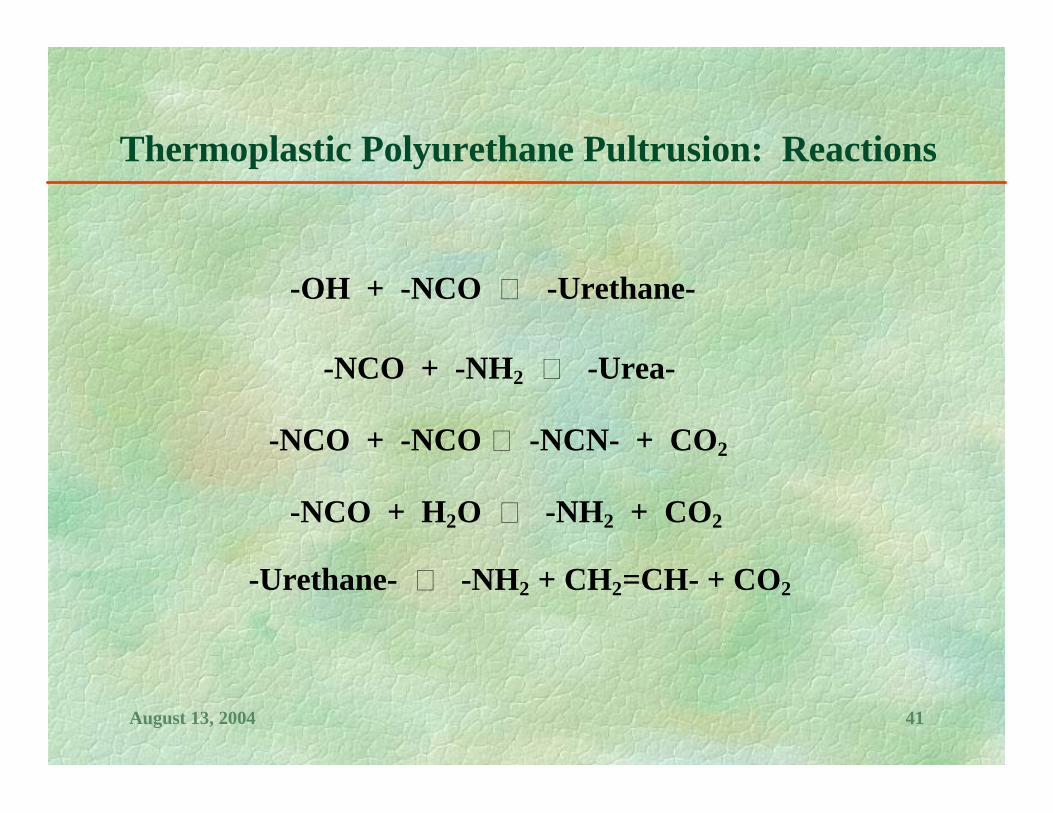
Thermoplastic Polyurethane Pultrusion: Reactions

-OH + -NCO -Urethane-

-NCO + -NCO -NCN- + CO2

-NCO + H2O -NH2 + CO2

-Urethane- -NH2 + CH2=CH- + CO2

-NCO + -NH2 -Urea-

August 13, 2004 42

Thermoplastic Polyurethane Pultrusion: Mw Prediction

Applied temperature profiles (left) all exhibit the same temperature rise and fall rates, but differ in length of the plateau that the temperature resides at prior to cooling and that determines the extruder residence time.

The assumed reaction mechanism was implemented with the dynamic Monte Carlo method. The starting Mw was ~75 kg/mole, and a shorter residence time was found to favor a higher final Mw. Snapshots of weight distributions of formed polymers at time 25 sec and 85 sec are shown at the right. See T. A. M. Verbrugge and C. F. J. den Doelder (to be published) for further details.

0

10000

20000

30000

40000

50000

60000

70000

80000

0 50 100 150 200 250 300

Time [s]

0

100

200

300

400

500

600

700

800

0

0.02

0.04

0.06

0.08

0.1

0.12

0.14

2.6 2.8 3.0 3.2 3.4 3.6 3.8 4.0 4.2 4.4 4.6 4.8 5.0 5.2 5.4

Log M [g/mol]

Time = 25 sec

Time = 85 sec

August 13, 2004 43

MODELING WATER VAPOR TRANSPORT

Determine the filler [Linde Type A (LTA) zeolite] loadings needed to “activate” a polyolefin/desiccant blend for water vapor transmission.

Schematic Illustration of Initial Morphological Hypothesis Micrograph

August 13, 2004 44

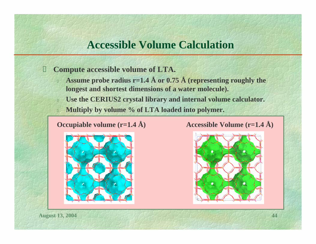
Accessible Volume Calculation

Compute accessible volume of LTA. Assume probe radius r=1.4 Å or 0.75 Å (representing roughly the

longest and shortest dimensions of a water molecule). Use the CERIUS2 crystal library and internal volume calculator. Multiply by volume % of LTA loaded into polymer.

Occupiable volume (r=1.4 Å) Accessible Volume (r=1.4 Å)

August 13, 2004 45

Water Vapor Transport Modeling Summary

Percolation Model for LTAin D2045A at 5% PEG

0

10

20

30

40

50

60

70

80

90

0 0.1 0.2 0.3 0.4 0.5 0.6

Vol % LTA

MV

TR

gm

/m^

2/d

ay @

7 m

il

0

0.05

0.1

0.15

0.2

0.25

Vo

l. %

Acc

essi

ble

MVTRprobe 1.4probe 0.75Linear (probe 1.4)Linear (probe 0.75)Expon. (MVTR)

The observed water vapor transmission rates were compared with the calculated water-accessible LTA zeolite volume fraction in the blends.

The sudden onset of water vapor transmission was seen to coincide simply with the percolation threshold for water accessibility with a probe radius of 1.4 Å, without the need to assume the existence of a “channel” morphology.

August 13, 2004 46

SUMMARY AND CONCLUSIONS

Polymer modeling has reached the state of maturity where it can serve as a powerful component of an industrial R&D program on polymer product and process development.

Such work, at its most effective, attempts to address all of the essential formulation, process and product issues within a multidisciplinary and multiscale modeling paradigm.

A few polymer modeling projects from Dow Chemical were reviewed to illustrate some of the many types of industrially relevant problems that can be solved.