arX

iv:1

009.

3402

v2 [

gr-q

c] 2

9 Ja

n 20

11

Polyhedra in loop quantum gravity

Eugenio Bianchia, Pietro Donaa,b and Simone Spezialea

aCentre de Physique Theorique∗, CNRS-Luminy Case 907, 13288 Marseille Cedex 09, Franceb Scuola Normale Superiore, Piazza dei Cavalieri 7, 56126 Pisa, Italy

February 1, 2011

Abstract

Interwiners are the building blocks of spin-network states. The space of intertwiners isthe quantization of a classical symplectic manifold introduced by Kapovich and Millson.Here we show that a theorem by Minkowski allows us to interpret generic configurationsin this space as bounded convex polyhedra in R3: a polyhedron is uniquely described bythe areas and normals to its faces. We provide a reconstruction of the geometry of thepolyhedron: we give formulas for the edge lengths, the volume and the adjacency of itsfaces. At the quantum level, this correspondence allows us to identify an intertwiner withthe state of a quantum polyhedron, thus generalizing the notion of quantum tetrahedronfamiliar in the loop quantum gravity literature. Moreover, coherent intertwiners result tobe peaked on the classical geometry of polyhedra. We discuss the relevance of this result forloop quantum gravity. In particular, coherent spin-network states with nodes of arbitraryvalence represent a collection of semiclassical polyhedra. Furthermore, we introduce anoperator that measures the volume of a quantum polyhedron and examine its relationwith the standard volume operator of loop quantum gravity. We also comment on thesemiclassical limit of spinfoams with non-simplicial graphs.

Contents

1 Introduction 2

2 The phase space of polyhedra 3

2.1 Convex polyhedra and Minkowski theorem . . . . . . . . . . . . . . . . . . . . . 32.2 Kapovich-Millson phase space as the space of shapes of polyhedra . . . . . . . 42.3 Classes of polyhedra with F faces . . . . . . . . . . . . . . . . . . . . . . . . . . 5

3 Polyhedra from areas and normals: reconstruction procedure 9

3.1 Lasserre’s reconstruction algorithm . . . . . . . . . . . . . . . . . . . . . . . . . 93.2 Volume of a polyhedron in terms of areas and normals . . . . . . . . . . . . . . 12

∗Unite Mixte de Recherche (UMR 6207) du CNRS et des Universites Aix-Marseille I, Aix-Marseille II et duSud Toulon-Var. Laboratoire affilie a la FRUMAM (FR 2291).

1

3.3 Adjacency matrix and the class of the polyhedron . . . . . . . . . . . . . . . . 143.4 Shape-matching conditions . . . . . . . . . . . . . . . . . . . . . . . . . . . . . 15

4 Relation to loop quantum gravity 16

4.1 The quantum polyhedron . . . . . . . . . . . . . . . . . . . . . . . . . . . . . . 164.2 Coherent intertwiners and semiclassical polyhedra . . . . . . . . . . . . . . . . 184.3 Coherent states on a fixed graph and twisted geometries . . . . . . . . . . . . . 19

5 On the volume operator 21

5.1 The volume of a quantum polyhedron . . . . . . . . . . . . . . . . . . . . . . . 215.2 LQG volume operator and the quantum polyhedron . . . . . . . . . . . . . . . 24

6 On dynamics and spin foams 26

7 Conclusions 28

1 Introduction

Loop quantum gravity (LQG) is a continuous theory, whose Hilbert space is the direct sumof spaces associated to graphs Γ embedded in a three-dimensional hypersurface, H = ⊕ΓHΓ.It is often convenient to consider a single graph Γ, and the associated Hilbert space HΓ. Thetruncation captures only a finite number of degrees of freedom of the theory. An importantquestion for us is whether these degrees of freedom can be “packaged” as to provide someapproximate description of smooth 3d geometries [1, 2]. We specifically think that it would beuseful to have a picture of the classical degrees of freedom captured by HΓ in terms of discretegeometries. Such knowledge is for instance relevant for the interpretation of semiclassical statesrestricted on HΓ.

As it turns out, useful insights can be gained looking at the structure of HΓ. It decomposesin terms of SU(2)-invariant spacesHF associated to each node of valence F . For a 4-valent node,it has been known for quite some time that an intertwiner represents the state of a “quantumtetrahedron” [3, 4], namely the quantization of the space of shapes of a flat tetrahedron inR3 with fixed areas. For a generic valence F , a natural expectation would be a relation topolyhedra with F faces, as mentioned in [5] and [1]. In this paper we clarify the details of thiscorrespondence.

There are two keys to our result. The first one is the fact that HF is the quantization of acertain classical phase space SF , introduced by Kapovich and Millson in [6]. The second is thefact that there is a unique bounded convex polyhedron with F faces of given areas associated toeach point of SF . This is guaranteed by an old theorem by Minkowski [7]. The correspondenceis up to a measure-zero subset of “degenerate” configurations, present also in the 4-valent case.Accordingly, we have the following relations:

polyhedra with F faces ←→ classical phase space SF ←→ intertwiner space HF .

2

An immediate consequence of these results is a complete characterization of coherent statesat a fixed graph: they uniquely define a collection of polyhedra associated to each node ofthe graph. This provides a simple and compelling picture of the degrees of freedom of HΓ

in terms of discrete geometries, which are associated with a parametrization of the classicalholonomy-flux variables in terms of the twisted geometries introduced in [1].

The paper is divided into two parts, concerning respectively the classical geometry of poly-hedra, and the notion of quantum polyhedron together with its relevance to loop gravity. Themotivation for the first part comes from the fact that polyhedra have a rich classical geometry.One of the reasons why the notion of quantum tetrahedron has been so fruitful in the devel-opement of loop gravity and spinfoams is the fact that everybody understands the geometryof a classical tetrahedron. To make the extension to higher valence as fruitful, we need first ofall to clarify a number of aspects of the geometry of polyhedra.

Minkowski’s theorem guarantees that a polyhedron can be reconstructed out of the areasand normals to its faces, just as it happens for the tetrahedron. The new feature here isthat there are many possible polyhedra with the same number of faces which differ in theircombinatorial structure, i.e. in the adjacency relations of the faces. In the first part of thepaper (sections 2 and 3) we focus entirely on the classical geometry of polyhedra, and collectand in some cases adapt various results known in the mathematical literature. We discuss thecombinatorial classes of polyhedra, and how the phase space of shapes at given areas can bedivided into regions of different classes. We show explicitly how a given configuration of areasand normals can be used to reconstruct the polyhedron geometry, including its edge lengths,volume and combinatorial class. Furthermore, we discuss certain shape matching conditions

which effectively restrict a collection of polyhedra to (a generalization of) Regge geometries.In the second part of the paper (sections 4 to 6) we discuss the quantum theory. We first

review the construction of the quantization map between the phase space SF and Hilbert spaceof intertwiners HF . This leads to the interpretation of an intertwiner state as the state ofa quantum polyhedron, and of coherent intertwiners [8, 9] as states describing semiclassicalpolyhedra. The relevance of polyhedra extend to the whole graph Hilbert space HΓ, via thetwisted geometries variables. The result provides an interpretation of coherent spin-networkstates in HΓ as a collection of semiclassical polyhedra.

Furthermore, we introduce a new operator which measures the volume of a quantum poly-hedron. Its definition is based on the knowledge of the classical system behind the intertwinerspace HF , and has the right semiclassical limit on nodes of any valence. We discuss its rela-tion with the standard volume operator of loop quantum gravity. Finally, we make some briefremarks on the polyhedral picture, Regge calculus and covariant spin foam models.

2 The phase space of polyhedra

2.1 Convex polyhedra and Minkowski theorem

A convex polyhedron is the convex hull of a finite set of points in 3d Euclidean space. It canbe represented as the intersection of finitely many half-spaces as

P ={x ∈ R

3 |ni · x ≤ hi, i = 1, . . . ,m}, (1)

3

where ni are arbitrary vectors, and hi are real numbers. The abstract description (1) is non-unique and redundant: the minimal set of half-spaces needed to describe a polyhedron corre-sponds to taking their number m equal to the number of faces F of the polyhedron. In thispaper we are interested in the description of a convex polyhedron with F faces in terms of vari-ables that have an immediate geometric interpretation: the areas of the faces of the polyhedronand the unit normals to the planes that support such faces.

Let us consider a set of unit vectors ni ∈ R3 and a set of positive real numbers Ai suchthat they satisfy the closure condition

C ≡F∑

i=1

Ai ni = 0. (2)

In the following, we will refer to this set as “closed normals”. A convex polyhedron with Ffaces having areas Ai and normals ni can be obtained in the following way. For each vectorni consider the plane orthogonal it. Then translate this plane to a distance hi from the originof R3. The intersection of the half-spaces bounded by the planes defines the polyhedron,ni · x ≤ hi. We can then adjust the heights so that hi = hi(A) so that the faces have areas Ai.

Remarkably, a convex polyhedron with such areas and normals always exists. Moreover, itis unique, up to rotations and translations. This result is established by the following theoremdue to H. Minkowski [7, 10]:

Theorem (Minkowski, 1897)

(a) If n1, . . . , nF are non-coplanar unit vectors and A1, . . . , AF are positive numbers such that

the closure condition (2) holds, than there exists a convex polyhedron whose faces have

outwards normals ni and areas Ai.

(b) If each face of a convex polyhedron is equal in area to the corresponding face with parallel

external normal of a second convex polyhedron and conversely, then the two polyhedra are

congruent by translation.

This unicity will play an important role in the following. Throughout the rest of the paper, weuse simply polyhedra to refer to bounded convex polyhedra.

2.2 Kapovich-Millson phase space as the space of shapes of polyhedra

Let us consider F vectors in R3 that have given norms A1, . . . , AF and such that they sum upto zero. The space of such vectors modulo rotations has the structure of a symplectic manifold[6] and is known as the Kapovich-Millson phase space1 SF ,

SF ={ni ∈ (S2)F | ∑F

i=1Aini = 0}/SO(3) . (3)

The Poisson structure on this 2(F−3)-dimensional space is the one that descends via symplecticreduction from the natural SO(3)-invariant Poisson structure on each of the F spheres S2.

1In [6] it is also called the space of shapes of (bended) polygons. To be precise, it is a symplectic manifoldup to a finite number of points, corresponding to configurations with one or more consecutive vectors collinear.

4

Action-angle variables for (3) are (F − 3) pairs (µi, θi) with canonical Poisson brackets,{µi, θj} = δij . Here µi is the length of the vector ~µi = A1n1 + . . . + Ai+1ni+1 (see Fig.1), andits conjugate variable θi is the angle between the plane identified by the vectors ~µi−1, ~µi andthe plane identified by the vectors ~µi, ~µi+1. At fixed areas, the range of each µi is finite.

OA1n1

A2n2

A3n3

A4n4

Figure 1: A polygon with side vectorsAini and the (F−3) independent diagonals. The space of possiblepolygons in R3 up to rotations is a (2F − 6)-dimensional phase space, with action-angle variables thepairs (µi, θi) of the diagonal lengths and dihedral angles. For non-coplanar normals, the same datadefines also a unique polyhedron thanks to Minkowski’s theorem.

Thanks to Minkowski’s theorem, a point in SF with non-coplanar normals identifies aunique polyhedron. Accordingly, we refer to (3) as the space of shapes of polyhedra at fixed

areas. Notice that (3) contains also configurations with coplanar normals: they can be thoughtof as “degenerate” polyhedra, obtained as limiting cases. The fact that the polyhedra withfaces of given areas form a phase space will be important in section (4.1) where we discuss theHilbert space of the quantum polyhedron.

2.3 Classes of polyhedra with F faces

The phase space SF has a rich structure: as we vary the normals of a polyhedron keepingits areas fixed, not only the geometry, but in general also the combinatorial structure of thepolyhedron changes; that is, the number of edges and the adjacency of faces. We refer tothe combinatorial structure as the class of the polyhedron. In other words, there are twocomponents to the shape of a polyhedron: its class, and its geometry (up to rotations) once thecombinatorial structure is fixed. The different classes of polyhedra correspond to the differenttessellations of a sphere having F faces. Which class is realized, depends on the specific valueof the normals. This is a point we would like to stress: one is not free to choose a class, andthen assign the data. It is on the contrary the choice of data that selects the class. This isan immediate consequence of Minkowski’s theorem. Accordingly, the phase space SF can bedivided into regions corresponding to the different classes of polytopes with F faces.

To visualize the class of a polyhedron it is convenient to use Schlegel diagrams [11, 10]. TheSchlegel diagram of a polyhedron is a planar graph obtained choosing a face f , and projectingall the other faces on f as viewed from above. See Fig.2 for examples.

To understand the division of SF into regions of different class, let us first give someexamples, and postpone general comments to the end of the Section. In the most familiarF = 4 case, there is no partitioning of S4: there is a unique tessellation of the sphere, the

5

Figure 2: Some examples of Schlegel diagrams. From left to right, a tetrahedron, a pyramid, a cubeand a dodecahedron.

tetrahedron, and it is well known that there is always a unique tetrahedron associated withfour closed normals. The first non-trivial case is F = 5, where there are two possible classes: atriangular prism, and a pyramid (see Fig. 3). Consider then the phase space S5. Minkowski’s

Dominant: Codimension 1:

Figure 3: Polyhedra with 5 faces: the two possible classes are the triangular prism (left panel) and thepyramid (right panel). The two classes differ in the polygonal faces and in the number of vertices.

theorem guarantees that the same set (Ai, ni) cannot be associated to both classes, thus eachpoint in S5 corresponds to a unique class. One might at first think that S5 can be more or lessequally divided among the two classes, but this is not the case. In fact, notice that the pyramidis just a special case of the prism, obtained by collapsing to a point one of the edges connectingtwo triangular faces. The existence of a pyramid then requires a non-trivial condition, i.e. thepresence of a 4-valent vertex. A moment of reflection shows that this condition can be imposedvia an algebraic equation on the variables. Hence the shapes corresponding to pyramids span acodimension one surface in S5. Generic configurations of areas and normals describe triangularprisms, and the pyramids are measure zero special cases. We call dominant the class of maximaldimensionality, e.g. the triangular prism here.

Let us move to F = 6, a case of particular interest since regular graphs in R3 are six-valent.There are seven different classes of polyhedra, see Fig.4. The most familiar one is the cuboid(top left of Fig.4), with its six quadrilateral faces. Remarkably, there is a further dominantclass: it is a “pentagonal wedge”, i.e. a polyhedron with two triangles, two quadrilaterals andtwo pentagons as faces (to visualize it, immagine a triangular prism planed down on a corner,so that a vertex is replaced by a triangle). The remaining five classes are subdominant, becausenon-trivial conditions are required for their existence. Subdominant classes have fewer verticesand thus can be seen as special cases with certain edges of zero length.2

2Among these, notice the class of codimension 3. It has six triangular faces and three four-valent vertices.This class is interesting in that it can be seen as two tetrahedra glued along a common triangle. Two arbitrarytetrahedra are defined by 12 independent numbers. In order for them to glue consistently and generate thispolyhedron, the shape of the shared triangle has to match. This shape matching requires three conditions (forinstance matching of the edge lengths), thus we obtain a 9-dimensional space of shapes. For fixed external areas,this is precisely the codimension 3 subspace in S6. Hence this class is a special case of two tetrahedra where

6

Dominant:

Codimension 1:

Codimension 2:

Codimension 3:

Figure 4: The seven classes of polyhedra with 6 faces, grouped according to the dimensionality of theirconfigurations.

From the above analysis, we expect that the phase space S6 can then be divided intoregions corresponding to the two dominant classes, separed by the subdominant ones. Thisis qualitatively illustrated in Figure 5. To confirm this picture, we performed some numerical

Figure 5: Pictorial representation of the phase space: it can be mapped into regions corresponding tothe various dominant classes (two in the example). The subdominant classes separe the dominant onesand span measure-zero subspaces.

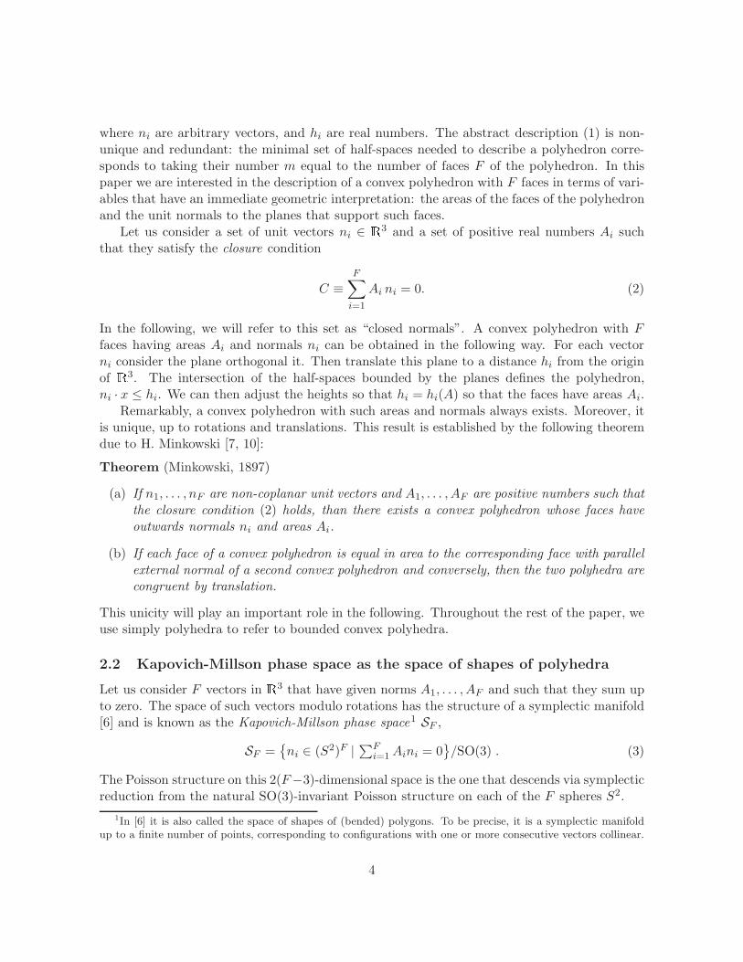
investigations. Using the reconstruction algorithm, which we introduce in the next Section, wecan assign a class to each point in S6. In Fig.6 we give an explicit example of a 2d and a 3dslice of the 6d space S6, which shows the subdivision into the two dominant classes.

After this brief survey of some specific examples, let us make some general statements.

• The phase space SF can be divided into regions corresponding to different classes. Thedominant classes, generically more than one, cover it densely, whereas the subdominantones span measure-zero subspaces. The dominant classes in phase space correspond topolyhedra with all vertices three-valent, that is the dual to the tessellation is a triangu-lation. This condition maximizes both the number of vertices, V = 3(F − 2), and edges,E = 2(F − 2). Subdominant classes are special configurations with some edges of zerolengths and thus fewer vertices.

• Since all classes correspond to tessellations of the sphere with F faces, they are connectedby Pachner moves [12]. The reader can easily find a sequence of moves connecting all

conditions are imposed for them to glue consistently.

7

Θ3

Μ3

Figure 6: Mappings of subspaces of S6 realized using the reconstruction algorithm of Section 3 andWolfram’s Mathematica. We subdivided the phase space into a regular grid, and had Mathematicacomputing the adjacency matrix of the area-normal configurations lying at the center of the cells. Thisassociates a unique class to each cell of the phase space. The information is colour-coded, cuboids inblue, pentagonal wedges in red. With this mapping of finite resolution we have measure-zero probabilityof hitting a subdominant class, thus the latter are absent in the figures. The holes are configurationsfor which our numerical algorithm failed. Concerning the specific values of the example, the areas aretaken to be (9, 10, 11, 12, 13, 13). In the left panel, we fixed µ1 = 15, θ1 = 7

10π, µ2 = 13, θ2 = 13

10π, and

plotted the remaining pair (µ3, θ3). In the right panel, we fixed µi = (15, 13, 17) and plotted the threeangles θi.

seven classes of Fig.4. To start, apply a 2-2 move to the upper edge of the inner squareof the cuboid to obtain the pentagonal wedge.

• The lowest-dimensional class corresponds to a maximal number of triangular faces, acondition which minimizes the number of vertices. When all the faces are triangular, thepolyhedron can be seen as a collection of tetrahedra glued together, and with matchingconditions imposed along all shared internal triangles.

2.3.1 Large F and the hexagonal dominance

The number of classes grows very fast with F (see for instance [13] for a tabulation). In theexamples above with small F , we have been able to characterize the class looking just at howmany faces have a certain valence. However as we increase F we find classes with the samevalence distribution, but which differ in the way the faces are connected. To distinguish theclasses one needs to identify the complete combinatorial structure of the polyhedron. Thisinformation is captured by the adjacency matrix, which codes the connectivity of the faces ofthe polyhedron. Below in Section 3.3 we will show how this matrix can be explicitly built as afunction of areas and normals, and give some explicit examples.

An interesting question concerns the average valence of a face, defined as 〈p〉 = 2E/F . Asimple estimate can be given using the fact that the boundary of any polyhedron is a tessellation

8

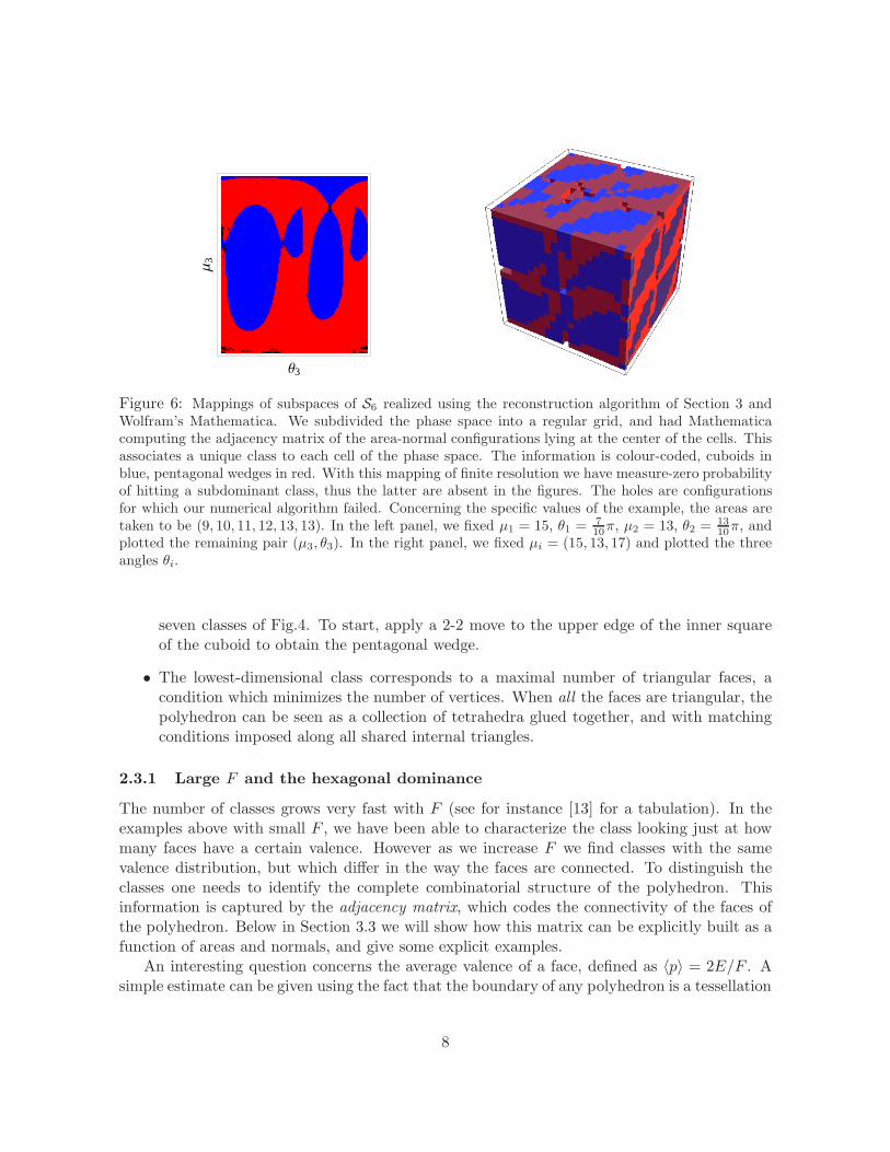
of the two-sphere, therefore by the Euler formula F − E + V = 2. For the dominant classes,which are dual to triangulations, the additional relation 2E = 3V holds, hence E = 3(F − 2)and we get 〈p〉 = 6(1 − 2/F ). For large F , we expect the polyhedron to be dominated byhexagonal faces. This expectation is immediately confirmed by a simple numerical experiment.The specimen in Figure 7, for instance, has F = 100 and 〈p〉 ∼ 5.88. Notice also from the

Figure 7: A polyhedron with F = 100 drawn with Wolfram’s Mathematica, using the reconstructionalgorithm. The example has all areas equals and normals uniformly distributed on a sphere. Noticethat most faces have valence 6, and that triangles are nowhere to be seen.

image that there are no triangular faces, consistently with the fact that they tend to minimizethe number of vertices and are thus highly non-generic configurations.

3 Polyhedra from areas and normals: reconstruction procedure

So far we have discussed how a point in SF specifies a unique polyhedron, and the existenceof different combinatorial structures. We now describe how the polyhedron can be explicitlyreconstructed from areas and normals. The reconstruction will allow us to evaluate completelyits geometry, including the lengths of the edges and the volume, and to identify its class throughthe adjacency matrix, thus being able to associate a class with each point of SF .

The main difficulty in developing a reconstruction algorithm is that, given the areas andthe normals, it is not known a priori which faces of the polyhedron are adjacent. The adjacencyrelations of the faces (and the combinatorial class of the polyhedron) are to be derived togetherwith its geometry. This can be done in two steps. The first step uses an algorithm due toLasserre [14] that permits to algebraically compute the lengths ℓij(h, n) of all the edges of thepolyhedron as defined by hi and ni, as in (1). The second step consists of solving a certainquadratic system to obtain the values of the heights hi for given areas.

3.1 Lasserre’s reconstruction algorithm

We now review Lasserre’s procedure, and adapt it to the three-dimensional case of interesthere. The basic idea of the reconstruction algorithm is to compute the length of an edge as

9

the length of an interval in coordinates adapted to the edge. Consider the i-th face. From thedefining inequalities (1), we know that points x ∈ R

3 on this face satisfy

ni · x = hi (4a)

nj · x ≤ hj , i 6= j. (4b)

We consider the generic case in which ni · nj 6= ±1 ∀i, j (these special configurations can beobtained as limiting cases). We introduce coordinates yi adapted to the face, that is

ni · yi = 0, yi = x− (x · ni)ni. (5)

Using (4a) we get x = hini + yi, which inserted in (4b) gives

yi · nj ≤ rij , i 6= j , (6)

where we have definedrij ≡ hj − (ni · nj)hi . (7)

Hence, the i-th face can be characterized either in terms of the x or the yi coordinates,{x · ni = hinj · x ≤ hj , i 6= j

−→{yi · ni = 0yi · nj ≤ rij(h, n), i 6= j

(8)

Notice that rij/√

1− (ni · nj)2 is the distance of the edge ij from the projection of the originon the i-th face.

The next step is to iterate this process and describe an edge in terms of its adapted coordi-nates. We start from the i-th face again, and assume that it is connected to the face j, so thatthe two faces share an edge. Points on the edge ij between the i-th and the j-th face satisfy

yi · ni = 0 (9)

yi · nj = rij (10)

yi · nk ≤ rik, k 6= i, j. (11)

As before, we introduce coordinates zij , adapted to the edge,

ni · zij = nj · zij = 0, zij = yi − [nj − (ni · nj)ni]yi · nj

1− (ni · nj)2. (12)

Using (10) we get that for a point in the edge

yi = [nj − (ni · nj)ni]hj − hi(ni · nj)1− (ni · nj)2

+ zij . (13)

Plugging this in (11) giveszij · nk ≤ bij,k, (14)

where we have defined

bij,k ≡ hk − (ni · nk)hi −(nj · nk)− (ni · nj)(ni · nk)

1− (ni · nj)2[hj − hi(ni · nj)] . (15)

10

Summarizing as before, going to adapted coordinates the edge is defined by

yi · ni = 0yi · nj = rij(h, n)yi · nk ≤ rik(h, n), k 6= i, j.

−→

zij · ni = 0zij · nj = 0zij · nk ≤ bij,k(h, n), i 6= j 6= k

(16)

At this point we are ready to evaluate the length of each edge. To that end, we parametrizethe zij coordinate vector in terms of its norm, say λ, and its direction which is given by thewedge product of the two normals,

zij = λni ∧ nj√

1− (ni · nj)2. (17)

If we defineaij,k ≡

ni ∧ nj · nk√1− (ni · nj)2

, (18)

we can rewrite the inequalities in (16) as

λaij,k ≤ bij,k. (19)

Finally, the length of the edge is the length of the interval determined by the tightest setof inequalities, i.e.

mink|aij,k>0

{bij,kaij,k

}− maxk|aij,k<0

{bij,kaij,k

}. (20)

Here the minimum is taken over all the k’s such that aij,k is positive, and the maximum over allthe k’s such that aij,k is negative. This quantity is symmetric [14] and satisfies a key property:it can be defined for any pair of faces ij, not only if their intersection defines an edge in theboundary of the polyhedron, and it is negative every time the edge does not belong to thepolyhedron [14]. Thanks to this property, we can consistently define the edge lengths for anypair of faces ij as

ℓij(h, n) = maxk

{0, mink|aij,k>0

{bij,kaij,k

}− maxk|aij,k<0

{bij,kaij,k

}}. (21)

The result is a matrix whose entries are the edge lengths (as a functions of the normals and theheights) if the intersection is part of the boundary of the polyhedron, and zero if the intersectionis outside the polyhedron.

This formula completes Lasserre’s algorithm, and permits one to reconstruct the polyhedronfrom the set (hi, ni). To achieve a description in terms of areas and normals, we need one morestep, that is an expression for the heights in terms of the areas. This can be done using (21) tocompute the areas of the faces. We consider the projection of the origin on the face, and useit to divide the face into triangles. Recall the Lasserre’s procedure has provided us with thedistance between an edge and the projected origin, see (8). We thus can write

Ai =1

2

F∑

j=1j 6=i

rij√1− (ni · nj)2

ℓij. (22)

11

Notice that both rij(h, n) from (7) and ℓij(h, n) from (21) are linear in the heights. Hence, thearea is a quadratic function,

Ai(h, n) =

F∑

j,k=1

M jki (n1, . . . , nF )hjhk, (23)

where Mi is a matrix depending only on the normals. This homogeneous quadratic system canbe solved for hi(A,n). The existence of a solution with hi > 0 ∀i is guaranteed by Minkowski’stheorem. However, the solution is not unique: in fact, we have the freedom of moving theorigin around inside the polyhedron, thus changing the value of the heights without changingthe shape of the polyhedron. A method which we found convenient to use is to determine asolution minimizing the function

f(hi) ≡∑

i

(Ai(h, n) −Ai)2 (24)

at areas and normals fixed, with Ai(h, n) given by (23). This is the method used in thenumerical investigations of Figs. 6 and 7.3

Finally, from the inverse we derive the lengths as functions of areas and normals, whichwith a slight abuse of notation we still denote in the same way,

ℓij(A,n) = ℓij(h(A,n), n). (25)

These expressions are well-defined and can be computed explicitly.

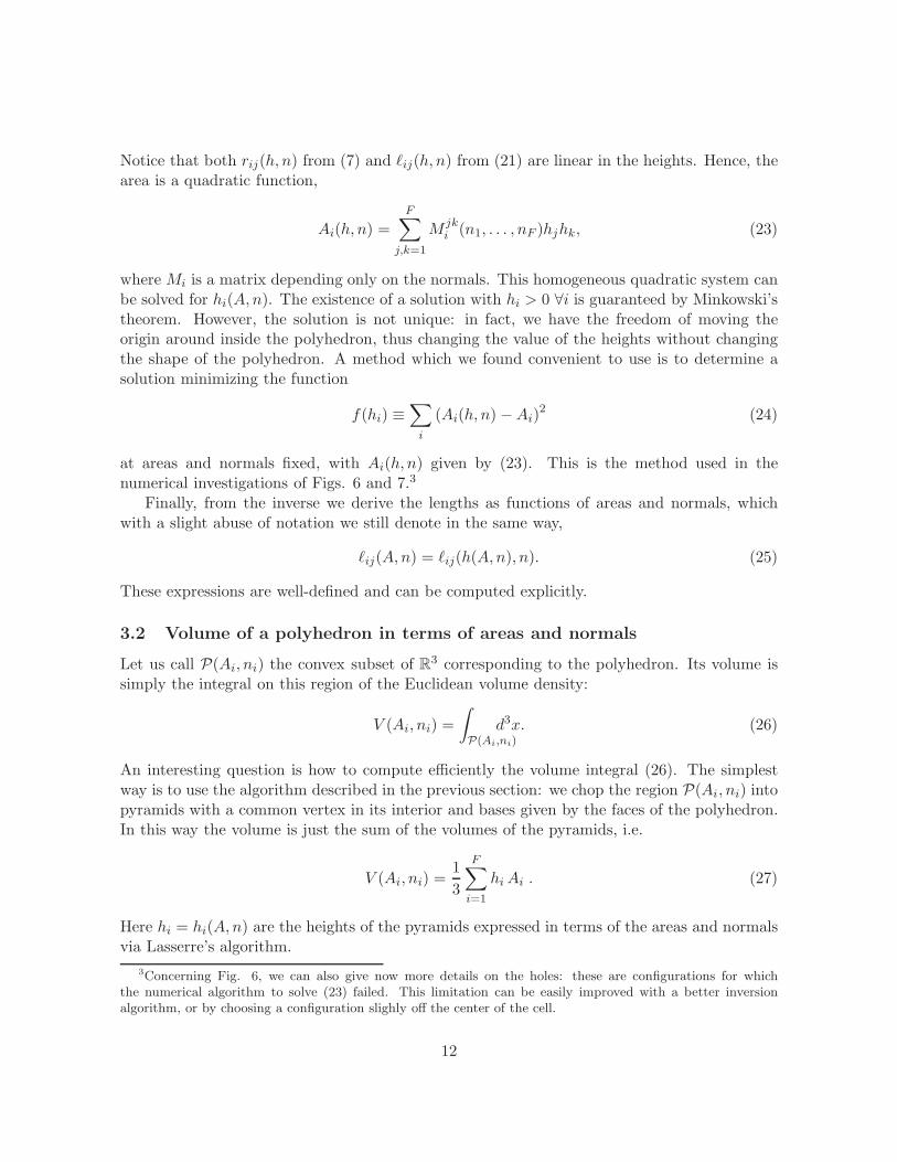
3.2 Volume of a polyhedron in terms of areas and normals

Let us call P(Ai, ni) the convex subset of R3 corresponding to the polyhedron. Its volume issimply the integral on this region of the Euclidean volume density:

V (Ai, ni) =

∫

P(Ai,ni)d3x. (26)

An interesting question is how to compute efficiently the volume integral (26). The simplestway is to use the algorithm described in the previous section: we chop the region P(Ai, ni) intopyramids with a common vertex in its interior and bases given by the faces of the polyhedron.In this way the volume is just the sum of the volumes of the pyramids, i.e.

V (Ai, ni) =1

3

F∑

i=1

hiAi . (27)

Here hi = hi(A,n) are the heights of the pyramids expressed in terms of the areas and normalsvia Lasserre’s algorithm.

3Concerning Fig. 6, we can also give now more details on the holes: these are configurations for whichthe numerical algorithm to solve (23) failed. This limitation can be easily improved with a better inversionalgorithm, or by choosing a configuration slighly off the center of the cell.

12

The volume can be used to define a volume function on the phase space SF . To that end,notice that (27) is not defined for configurations with coplanar normals, which on the otherhand do enter SF . However, it can be straightforwardly extended to a function on the wholeSF by defining it to be zero for coplanar configurations. Furthermore, the resulting phase spacefunction is continuous.4 Since the volume is manifestly invariant under rotations, it can alsobe written as a function of the reduced phase space variables only, that is, V (Ai, µk, θk). Todo so explicitly, one uses the relation ni = ni(µk, θk), which is straightforward to derive once areference frame is chosen.

The volume of the polyhedron as a function of areas and normals has a number of interestingproperties:

C1. Non-negative phase-space function. The volume is by construction non-negative, and atgiven areas, it vanishes only when the normals ni lie in a plane. This in particular impliesthat the volume vanishes for F = 2 and 3.

C2. Boundedness. For fixed areas Ai, the volume is a bounded function of the normals. Wecall Vmax(Ai) the volume of the polyhedron with maximum volume,5

Vmax(Ai) ≡ supni

{V (Ai, ni)} . (28)

In particular, Vmax(Ai) is smaller that the volume of the sphere that has the same surfacearea as the polyhedron. Therefore we have the bound

0 ≤ V (Ai, ni) <

(∑iAi

) 32

3√4π

. (29)

C3. Face-consistency. If we set to zero one of the areas such that the result is still a non-degenerate polyhedron, the function (27) automatically measures the volume of the re-duced polyhedron with F − 1 faces.

In conclusion, a point in SF determines uniquely the whole geometry of a polyhedron andin particular its edge-lengths ℓij (21) and its volume (27).6 Now we show how these data canbe used to identify the class of the polyhedron.

4In order to to see this, one shows that the limit of coplanar normals exists and the volume tends to zero inthis limit. From property (C3) – see below, a general F -valent coplanar configuration can be obtained from aF + 1 configuration in the limit of zero base’s area.

5Notice that there can be more than one polyhedron that attains maximum volume. For instance, in the caseF = 4, there are two parity-related tetrahedra with maximal volume.

6It is worth adding that the problem of computing the volume of a given polyhedron is a complex and wellstudied topic in computational mathematics [15, 16], hence better procedures than the one used here could inprinciple be found. However, the usual starting point for common algorithms is the knowledge of the coordinatesof vertices, or the system of inequalities (1). Therefore the methods need to be adapted to obtain formulas interms of areas and normals. The main difficulty is clearly that the adjacency relations of the faces are tobe derived together with the geometry. We found Lasserre’s algorithm to be the most compatible with thesenecessities, thanks to the fact that the lengths are reconstructed algebraically. Numerical algorithms for thevolume and shape reconstruction from areas and normals are developed in the study of extended Gaussianimages in informatics [17], however there are no analytical results.

13

3.3 Adjacency matrix and the class of the polyhedron

The adjacency matrix A of the polyhedron is defined as

Aij =

{1 if the faces i and j are adjacent0 otherwise

i, j = 1, . . . , F (30)

Notice that Aij coincides with the matrix ℓij in (21) with all the non-zero entries normalizedto 1: the recontruction algorithm gives us the adjacency matrix for free.

The symmetric matrix Aij contains information on the connectivity of the faces as well ason the valence of each face, thus the class of the polyhedron can be identified uniquely from it.The valence pi of the face i can be extracted taking the sum of the columns for each row,

pi =

F∑

j=1

Aij . (31)

For example, for the two classes with F = 5 of Fig.3 we have

−→ A =

0 0 1 1 10 0 1 1 11 1 0 1 11 1 1 0 11 1 1 1 0

−→ p = (3, 3, 4, 4, 4)

−→ A =

0 1 1 1 11 0 1 0 11 1 0 1 01 0 1 0 11 1 0 1 0

−→ p = (4, 3, 3, 3, 3)

From graph theory [18], we known that (30) has a number of interesting properties thatcan be related to the geometrical parameters of the polyhedron. For instance, the number ofwalks from the face i to the face j of length r is given by the matrix elements of the r-th power(Ar)ij . From this property we deduce that the number E of edges of the polyhedron is

E =1

2TrA2 =

1

2

∑

i

pi. (32)

This expression generalizes the value E = 3(F − 2) valid for the dominant classes.Higher traces are related to the number of loops of a given lengh. For instance, the number

of closed loops of length 3 is given by (1/6)TrA3.Through the adjacency matrix, obtained via the reconstruction procedure, areas and nor-

mals identify a unique class, and thus permits the division of SF .

14

3.4 Shape-matching conditions

Knowing the complete geometry of the polyhedra allows us also to address the following sit-uation. Suppose that we are given two polyhedra in terms of their areas and normals, andthat we want to glue them by a common face. Even if we choose the area of the common faceto be the same, there is no guarantee that the shape of the face will match: The two sets ofdata will in general induce different shapes of the face. That is, the face has the same area butit can be two different polygons altogether. In order to glue the polyhedra nicely, one needsshape matching conditions guaranteeing that the shared face has the same geometry in bothpolyhedra.

If both polyhedra are tetrahedra, the problem has been solved in [19]. One uses the fact thatthe shape of the common triangle matches if two lengths, or two internal angles, are the same.The internal angles α can be expressed in terms of the 3d dihedral angles of the tetrahedronas follows,

cosαijk =cosφij + cosφik cosφjk

sinφik sinφjk. (33)

Here the faces i, j and k all share a vertex, and αijk is the angle between the edge ij and theedge ik inside the triangle i. Consider now the adjacent tetrahedron. Its geometry induces forthe same angle the value

cosαij′k′ =cosφ′ij′ + cosφ′ik′ cosφ

′j′k′

sinφ′ik′ sinφ′jk′

. (34)

Hence, for the shape to match it is sufficient to require

Ckl,ij(φ) ≡ cosαijk − cosαij′k′ = 0 (35)

for two of the three angles of the triangle. These shape matching conditions are conditionson the normals of the two tetrahedra. See left panel of Figure 8 for an illustration of theserelations.

i

jk

k’ j’

i

Figure 8: The geometric meaning of equation (35): the 2d angle αij,kl belonging to the shaded trianglecan be expressed in terms of 3d angles associated the thick edges of the tetrahedron k, or equivalentyof the tetrahedron l.

15

The simplicity of the conditions (35) is a consequence of the fact that two triangles withthe same area are congruent if two angles match. For the general case, the face to glue is nowa polygon and the number of conditions greater. One needs to make sure that the valence pof the polygon is the same. Then, the number of independent parameters of a polygon on theplane is 2p − 3, hence giving the edge lengths is not enough, and p − 2 additional conditionsare needed. A convenient procedure is the following. Identify the faces of the two polyhedrathat, having the same area, we want to match. From the reconstruction algorithm, we knowthe edge lengths ℓij of the face viewed from one polyhedron. Then, for all j such that ℓij 6= 0,we consider the face normals nj projected on the plane of the i-th face,

nj =nj − (ni · nj)ni|nj − (ni · nj)ni|

=nj − cosφijni

sinφij. (36)

The set (ℓj, nj) defines a unique polygon in the plane identified by ni, thanks to a two-dimensional version of Minkowski’s theorem. Then, we do the same with the second poly-hedron, obtaining a second set (ℓ′j , n

′j) living in the plane identified by n′i. Finally, the shape

matching conditions consist of imposing the equivalence of these two flat polygons up to rota-tions in three-dimensional space. Notice that the shape matching are now conditions on boththe normals and the areas of the two polyhedra.

4 Relation to loop quantum gravity

Thus far we have been discussing classical properties of polyhedra. In the rest of the paper,we discuss the relevance of polyhedra for loop quantum gravity. The relation comes from thefollowing two key results:

(i) Intertwiners are the building blocks of spin-network states, an orthonormal basis of theHilbert space of loop quantum gravity [20, 21]

(ii) Intertwiners are the quantization of the phase space of Kapovich and Millson [22, 9, 23](see also [24, 25]), i.e. of the space of shapes of polyhedra with fixed areas discussed inthe previous sections.

Therefore an intertwiner can be understood as the state of a quantum polyhedron, and spin-network states as a collection of quantum polyhedra associated with each vertex.

In this section we review how (ii) and the notion of quantum polyhedron are established,observe that coherent intertwiners are peaked on the geometry of a classical polyhedron anddiscuss the relevance of this fact for the relation between semiclassical states of loop quantumgravity and twisted geometries.

4.1 The quantum polyhedron

Let us consider the space of vectors in 3d Euclidean space with norm j. This is a phase space,the Poisson structure being the rotationally invariant one proper of the 2-sphere S2

j of radius j.

16

As is well known, its quantization7 is the representation space V (j) of SU(2). We are interestedin the phase space SF , that is the space of F vectors that sum to zero, up to rotations. ThePoisson structure on SF is obtained via the symplectic reduction of the Poisson structureon the product of F spheres of given radius. Thanks to Guillemin-Sternberg’s theorem thatquantization commutes with reduction,8 we can quantize first the unconstrained phase space×iS2

ji, and then reducing it at the quantum level extracting the subspace of ⊗iV (ji) that is

invariant under rotations. This gives precisely the intertwiner space HF = Inv[⊗Fi=1 V

(ji)].

The situation is summarized by the commutativity of the following diagram,

×iS2ji−→ ⊗iV ji

Symplectic reduction ↓ ↓ Quantum reduction

SF −→ HF

The correspondence between classical quantities and their quantization is the following: upto a dimensionful constant, the generators ~Ji of SU(2) acting on each representation space V (ji)

are understood as the quantization of the vectors Aini. In LQG the dimensionful constant ischosen to be the Immirzi parameter γ times Planck’s area 8πL2

P ,

Aini −→ Ei = 8πγL2P~Ji. (37)

The closure condition (2) on the normals of the polyhedron is promoted to an operator equation,

F∑

i=1

~Ji = 0. (38)

This condition defines the space of intertwiners, and corresponds to the Gauss constraint ofclassical General Relativity in Ashtekar-Barbero variables.

One can then proceed to associate operators to geometric observables through the quanti-zation map (37). The area of a face of the quantum polyhedron is

Ai =

√Ei · Ei = 8πγL2

P

√ji(ji + 1) (39)

and produces an equispaced quantization of the area Ai ∼ ji for large spins, i.e. up to quantumcorrections. Notice that an ordering can be chosen so that the area is exactly Ai = 8πγL2

P ji.This ordering will be considered below to simplify the construction of the volume operator.

The scalar product between the generators of SU(2) associated to two faces of the polyhe-dron measures the angle θij between them [27],

θij = arccos~Ji · ~Jj√

ji(ji + 1) jj(jj + 1). (40)

7Notice that, as usual, the quantum theory requirers the quantization of some classical quantities. In thiscase the norm of the vector has to be a half-integer j, the spin.

8For the general theory see [26], for details on the application to the current system see [4] and in particular [9].

17

Notice that the angle operators do not commute among themselves, therefore it is not possibleto find a state for a quantum polyhedron that has a definite value of all the angles between itsfaces. Moreover, the adjacency relations of the faces is not prescribed a priori, thus θij might noteven be a true dihedral angle of the polygon. Therefore an eigenstate of a maximal commutingset of angles is far from the state of a classical polyhedron: it is an infinite superposition ofpolyhedra of different shapes, including different combinatorial classes. Semiclassical states fora quantum polyhedron are discussed in the next section.

4.2 Coherent intertwiners and semiclassical polyhedra

Coherent intertwiners for HF were introduced in [8] and furtherly developed in [9, 23] (forprevious related work, see [28]). These Livine-Speziale (LS) coherent intertwiners are definedas the SU(2)-invariant projection of a tensor product of states |ji, ni〉 ∈ V (ji),

||ji, ni〉 ≡∫

dg D(j1)(g)|j1, n1〉 · · ·D(jF )(g)|jF , nF 〉. (41)

The states |j, n〉 are SU(2) coherent states peaked on the direction n of the spin [29, 30],

〈j, n| ~J |j, n〉 = jn. (42)

In (41), the unit-vectors ni can be assumed to close,∑

i jini = 0. The reduced states are stillan overcomplete basis of HF , as a consequence of the Guillemin-Sternberg theorem [9, 31].

Coherent intertwiners are semiclassical states for a quantum polyhedron: the areas aresharp, and the expectation value of the non-commuting angle operators θij reproduces theclassical angles between faces of the polyhedron in the large spin limit,

〈ji, ni|| cos θij ||ji, ni〉〈ji, ni||ji, ni〉

≈ ni · nj. (43)

Moreover, the dispersions are small compared to the expectation values.A useful fact is that coherent intertwiners can be labeled directly by a point in the phase

space SF of Kapovich and Millson, and therefore by a unique polyhedron. This provides aresolution of the identity in intertwiner space as an integral on SF . To realize this reduction,it is convenient to parametrize SF via F − 3 complex numbers Zk, instead of (µk, θk). Let uschoose an orientation in R3 and consider the stereographic projection zi of the unit-vectors niinto the complex plane.9 The F − 3 complex variables Zk are the cross-ratios [9]

Zk =(zk+3 − z1)(z2 − z3)(zk+3 − z3)(z2 − z1)

, k = 1, . . . , F − 3. (44)

9The relation between the unit-vector n = (nx, ny , nz) and the stereographic projection is

z = −nx − iny

1− nz

= − tanθ

2e−iφ,

where θ and φ are the zenith and azimuth angles of S2, and we have chosen to project from the south pole.

18

Given an orientation in R3, a set of normals ni that satisfy the closure condition (2) can beobtained as a function of the cross-ratios,

ni = ni(Zk) . (45)

Coherent intertwiners can then be obtained via geometric quantization [9]: they are labeledby the variables Zk, that is |ji, Zk〉, and are equal to the states ||ji, ni〉| = |ji, ni(Zk)〉 up toa normalization and phase.10 The resolution of the identity is given by an integral over thevariables Zk, 1HF

=

∫CF−3

dµ(Zk) |ji, Zk〉〈ji, Zk| , (46)

where the integration measure dµ(Zk) = Kji(Zk, Zk)∏k d

2Zk depends parametrically on thespins ji and is given explicitly in [9]. The relevance of this formula for the following discussionis that it provides a resolution of the identity in intertwiner space as a sum over semiclassicalstates, each one representing a classical polyhedron: the intertwiner space can be fully describedin terms of polyhedra.11

4.3 Coherent states on a fixed graph and twisted geometries

The states |ji, Zk〉 provide coherent states for the space of intertwiners only, and should not beconfused with coherent spin-network states for loop quantum gravity. Nevertheless, classicalpolyhedra and coherent intertwiners are relevant to the full theory, as we now discuss.

To relate polyhedra to loop quantum gravity, consider a truncation of the theory to asingle graph Γ, with L links and N nodes. The associated gauge-invariant Hilbert space HΓ =L2[SU(2)

L/SU(2)N ] decomposes in terms of intertwiner spaces HF (n) ≡ Inv[⊗l∈nV (jl)] as

HΓ = ⊕jl(⊗nHF (n)

). (48)

This Hilbert space is the quantization of a classical space12 SΓ = T ∗SU(2)L//SU(2)N , whichcorresponds to (gauge-invariant) holonomies and fluxes associated with links and dual faces ofthe graph. The double quotient // means symplectic reduction. The key result is that thisspace admits a decomposition analogous to (48). In fact, it can be parametrized as the followingCartesian product [1],

SΓ =×l

T ∗S1×n

SF (n), (49)

10The states |ji, Zk〉 also define an holomorphic representation of the quantum algebra of functions ψ(Zk) ≡〈ji, Zk|ψ〉, see [23]. We will not use this representation in this paper.

11Recently [5, 32, 33] attention has been given to a second space for which polyhedra are relevant. This is asum of intertwiner spaces such that the total spin is fixed,

HJ = ⊕j1..jF∑i ji=J

Inv[

⊗Fi=1 V

(ji)]

. (47)

The interest in this space is that it is a representation of the unitary group U(F). Vectors in this space representquantum polyhedra with fixed number of faces and fixed total area, but fuzzy individual areas as well as shapesas before. Coherent states for (47) can be built using U(F) coherent states [32]. These are also peaked onclassical polyhedra like the LS states (41), thus the results in this paper are relevant for them as well.

12Again, this is a symplectic manifold up to singular points [34].

19

where T ∗S1 is the cotangent bundle to a circle, F the valence of the node n, and SF is thephase space of Kapovich and Millson.

The parametrization is achieved through an isomorphism between holonomy-fluxes and aset of variables dubbed “twisted geometries”. These are the assignment of an area Al and anangle ξl to each link, and of F normals ni, satisfying the closure condition (2), to each node. See[1, 2] for details and discussions. In this parametrization, a point of SΓ describes a collectionof polyhedra associated to each node. The two polyhedra belonging to nodes connected by alink l share a face. The area of this face is uniquely assigned to both polyhedra Al (notice thatthis fact alone does not imply that the shape of the face matches – more on this below). Theextra angles ξl carry information on the extrisic geometry between the polyhedra.

The isomorphism (49) and the unique correspondence between closed normals and polyhe-dra means that each classical holonomy-flux configuration on a fixed graph can be visualized as

a collection of polyhedra, together with a notion of parallel transport between them. Just as theintertwiners are the building blocks of the quantum geometry of spin networks, polyhedra arethe building blocks of the classical phase space (49) in the twisted geometries parametrization.

What is the relevance of this geometric construction to the quantum theory? Coherentstates for loop quantum gravity have been introduced and extensively studied by Thiemannand collaborators [35, 36, 34]. Although the states for the full theory have components on eachgraph, one needs to cut off the number of graphs to make them normalizable. In practice, itis often convenient to truncate the theory to a single graph. This truncation provides a usefulcomputational tool, to be compared to a perturbative expansion, and has found many appli-cations, from the study of propagators [37] to cosmology [38]. In many of these applications,control of the semiclassical limit requires a notion of semiclassical states in the truncated spaceHΓ. The truncation can only capture a finite number of degrees of freedom, thus coherentstates in HΓ are not peaked on a smooth classical geometry. Twisted geometries offer a wayto see them as peaked on a discrete geometry, to be viewed as an approximation of a smoothgeometry on a cellular decomposition dual to the graph Γ. The above results provide a com-pelling picture of these twisted geometries in terms of polyhedra, and thus of coherent statesas a collection of semiclassical polyhedra.

There is one subtlety with this geometric picture that should be kept in mind, which justifiesthe name “twisted” geometries: they define a metric which is locally flat, but discontinuous. Tounderstand this point, consider the link shared by two nodes. Its dual face has area proportionalto Al. However, the shape of the face is determined independently by the data around eachnode (i.e. the normals and the other areas), thus generic configurations will give two differentshapes. In other words, the reconstruction of two polyhedra from holonomies and fluxes doesnot guarantee that the shapes of shared faces match. Hence, the metric of twisted geometriesis discontinuous across the face [1, 2].13 See left panel of Figure 8.

One can also consider a special set of configurations for which the shapes match, see rightpanel of Figure 8. This is a subset of the phase space SΓ where the shape matching conditions,discussed earlier in Section 3.4, hold. This subset corresponds to piecewise flat and continuous

metrics. For the special case in which all the polyhedra are tetrahedra, this is the set-up

13Aspects of this discontinuity have been discussed also in [39, 40]

20

of Regge calculus, and those holonomies and fluxes indeed describe a 3d Regge geometry:twisted geometries with matching conditions amount to edge lengths and extrinsic curvaturedihedral angles [1, 2]. This relation between twisted geometry and Regge calculus implies thatholonomies and fluxes carry more information than the space of Regge calculus. This is not incontradiction with the fact that the Regge variables and the LQG variables on a fixed graphboth provide a truncation of general relativity: simply, they define two distinct truncations ofthe full theory. See [2] for a discussion of these aspects.

For an arbitrary graph, the shape-matching subset describes a generalization of 3d Reggegeometry to arbitrary cellular decompositions. In this case however the variables are not equiv-alent any longer to edge lengths, since as already discussed these do not specify uniquely thegeometry of polyhedra. Rather, such cellular Regge geometry must use areas and normals asfundamental variables.

Finally, let us make some comments on the coherent states themselves. The discussion sofar is largely independent of the details of the coherent states on HΓ. All that is required isthat they are properly peaked on a point in phase space. The states most commonly used arethe heat-kernel ones of Thiemann and collaborators. Notice that these are not written in termsof the LS coherent intertwiners (41). Nevertheless, it was shown in [41] that they do reproducecoherent intertwiners in the large area limit. Alternative coherent states based directly oncoherent intertwiners appear in [42]. These results show that coherent intertwiners can be usedas building blocks of coherent spin networks.

5 On the volume operator

At the classical level, the volume of a polyhedron is a well-defined quantity. In this section weinvestigate the quantization of this quantity and its relation with the volume operators used inloop quantum gravity.

5.1 The volume of a quantum polyhedron

Let us consider the phase space SF of polyhedra with F faces of given area. The volume of thepolyhedron is a well-defined function on this phase spase, as discussed in Section 3.2. Coherentintertwiners provide a natural tool to promote this quantity to an operator in HF .

In the following we use the parametrization of the phase space SF in terms of the cross ratiosZk. In particular, the F normals ni are understood as functions of the cross-ratios, ni(Zk).Accordingly we call V (ji, Zk) the volume of a polyhedron with faces of area Ai(ji) = 8πγL2

P jiand normals ni(Zk),

V (ji, Zk) ≡ V (A(ji), n(Zk)) . (50)

For simplicity we assume an ordering of operators such that the area is linear in the spin,but the above expression, and the following construction, can be immediately applied to otherpossibilities.

Let us consider now the Hilbert space of intertwiners HF associated to the phase space SF .The volume of a quantum polyhedron can be defined in terms of coherent intertwiners |ji, Zk〉

21

and of the classical volume as follows:

V =

∫dµ(Zk) V (ji, Zk) |ji, Zk〉〈ji, Zk| . (51)

This integral representation of the operator in terms of its classical version14 is of the kindconsidered originally by Glauber [45] and Sudarshan [46]. It has a number of interestingproperties that we now discuss:

Q1. The operator V is positive semi-definite, i.e.

〈ψ|V |ψ〉 =∫dµ(Zk) V (ji, Zk) |〈ji, Zk|ψ〉|2 ≥ 0 , (52)

for every |ψ〉 in H. This is a straightforward consequence of the fact that the classicalvolume is a positive function, V (ji, Zk) ≥ 0. Furthermore, V vanishes for F = 2 and 3.

Q2. V is a bounded operator in HF . Its norm ||V || = supψ〈ψ|V |ψ〉/〈ψ|ψ〉 is bounded fromabove by the maximum value of the classical volume of a polyhedron with fixed areas,

〈ψ|V |ψ〉〈ψ|ψ〉 =

∫dµ(Zk) V (ji, Zk) |〈ji, Zk|ψ〉|2 ≤ sup

Zk

{V (ji, Zk)} ≡ Vmax(ji) . (53)

Q3. 0-spin consistency. Let us consider the operator V defined on the Hilbert space HF+1

associated to spins j1, . . . , jF , jF+1, and the one defined on the Hilbert space HF associ-ated to spins j1, . . . , jF . When the spin jF+1 vanishes, the two operators coincide. Thisis a consequence of the fact that the classical volume of a polyhedron with F + 1 facescoincides with the volume of a polyhedron with F faces and the same normals when oneof the areas is sent to zero.

These three properties are the quantum version of C1, C2, C3 discussed in Section 3.2. More-over, using the fact that for large spins two coherent intertwiners become orthogonal,

|〈ji, Zk|ji, Z ′k〉|2 → δ(Zk, Z

′k), (54)

we have that the expectation value 〈V 〉 of the volume operator on a coherent state |ji, Zk〉reproduces the volume of the classical polyhedron with shape (ji, Zk),

〈V 〉 ≡ 〈ji, Zk|V |ji, Zk〉〈ji, Zk|ji, Zk〉≈ V (Ai(ji), ni(Zk)). (55)

14In the literature [29], the classical function V (ji, Zk) is called the P -symbol of the operator V . On the otherhand, the expectation value of the operator V on a set of coherent states, i.e.

Q(ji, Zk) ≡ 〈ji, Zk|V |ji, Zk〉 ,

is called the Q-symbol. When the P -symbol and the Q-symbol of an operator exist, then the operator is fullydetermined by either of them. The properties of these symbols and of the operator they define have been studiedby Berezin in [43, 44]

22

This fact allows to estimate the largest eigenvalue of the volume: in the large spin limit, thelargest eigenvalue is given by Vmax(Ai), the volume of the largest polyhedron in SF .

The spectrum of the operator V can be computed numerically. Let us focus on the caseF = 4 for concreteness. The matrix elements of V in the conventional recoupling basis aregiven by

Vkk′ = 〈ji, k|V |ji, k′〉 =∫

dµ(Z)V (ji, Z) 〈ji, k|ji, Z〉〈ji, Z|ji, k′〉. (56)

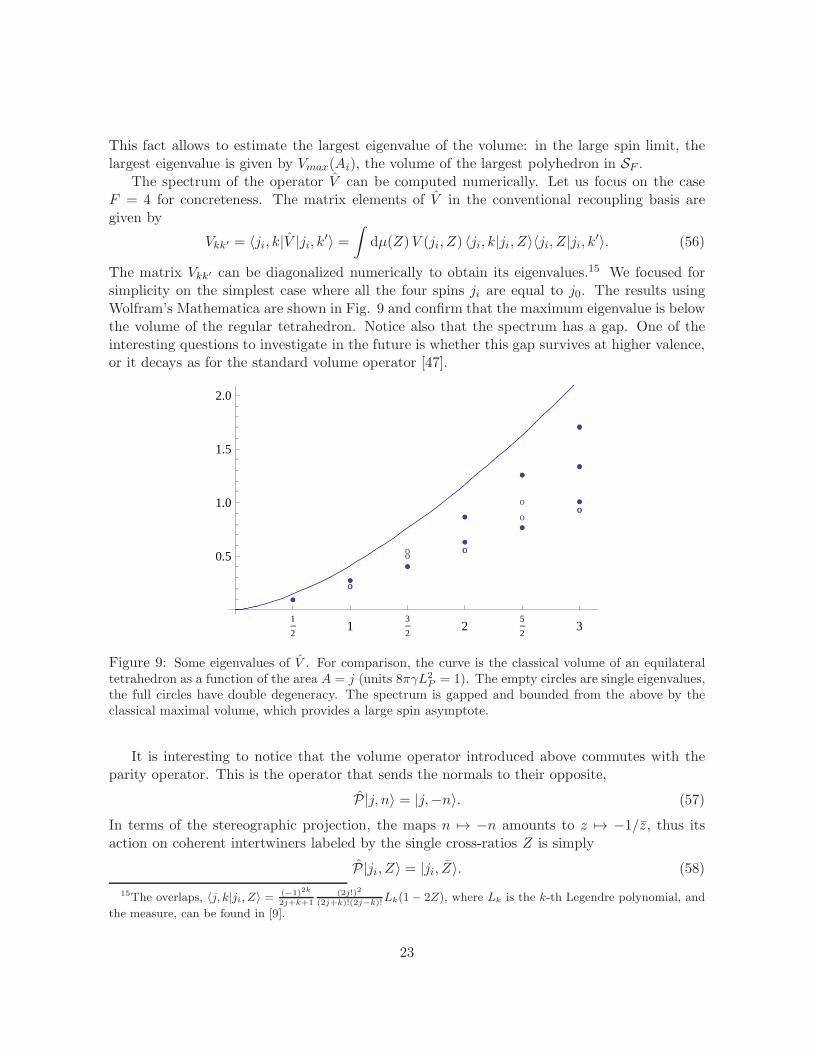
The matrix Vkk′ can be diagonalized numerically to obtain its eigenvalues.15 We focused forsimplicity on the simplest case where all the four spins ji are equal to j0. The results usingWolfram’s Mathematica are shown in Fig. 9 and confirm that the maximum eigenvalue is belowthe volume of the regular tetrahedron. Notice also that the spectrum has a gap. One of theinteresting questions to investigate in the future is whether this gap survives at higher valence,or it decays as for the standard volume operator [47].

••••oo

oo••

••••oo

••

••

o

o

••

••

••oo

1

21

3

22

5

23

0.5

1.0

1.5

2.0

Figure 9: Some eigenvalues of V . For comparison, the curve is the classical volume of an equilateraltetrahedron as a function of the area A = j (units 8πγL2

P = 1). The empty circles are single eigenvalues,the full circles have double degeneracy. The spectrum is gapped and bounded from the above by theclassical maximal volume, which provides a large spin asymptote.

It is interesting to notice that the volume operator introduced above commutes with theparity operator. This is the operator that sends the normals to their opposite,

P|j, n〉 = |j,−n〉. (57)

In terms of the stereographic projection, the maps n 7→ −n amounts to z 7→ −1/z, thus itsaction on coherent intertwiners labeled by the single cross-ratios Z is simply

P|ji, Z〉 = |ji, Z〉. (58)

15The overlaps, 〈j, k|ji, Z〉 = (−1)2k

2j+k+1(2j!)2

(2j+k)!(2j−k)!Lk(1− 2Z), where Lk is the k-th Legendre polynomial, and

the measure, can be found in [9].

23

Notice that V (ji, Zk) = V (ji, Zk) thanks to the invariance of the classical volume under parity.Moreover the measure dµ(Zk) is invariant under the transformation Zk → Zk. As a result, theoperator (51) commutes with parity,

PV P† =∫

dµ(Z)V (ji, Z)|ji, Z〉〈ji, Z| =∫

dµ(Z)V (ji, Z)|ji, Z〉〈ji, Z| = V . (59)

This explains the degeneracies seen in the spectrum.

Clearly, there are other possibilities for the volume of a quantum polyhedron. All of themshare the same classical limit, but can have a different spectrum for small eigenvalues. An

interesting variant isˆV =

√|U |, where U is the oriented-volume square operator, defined as

U =

∫dµ(Zk) s(Zk)V

2(ji, Zk) |ji, Zk〉〈ji, Zk|. (60)

Here s(Zk) is the parity of the polyhedron, i.e. s(Zk) = ±1 and s(Zk) = −s(Zk).The operator U anticommutes with the parity, and so does

ˆV . Therefore, under the as-

sumption that the spectrum is non-degenerate, we have that the eigenvalues appear in pairs±u. In particular, a zero eigenvalue is present when the Hilbert space HF is odd-dimensional.This operator is similar in spirit to the the volume of a quantum tetrahedron introduced by

Barbieri [3], VB = (8πγ)32L3

P

√23

√|J1 · (J2 × J3)|. In Fig. 10 we show some eigenvalues of

ˆV

and a comparison with VB .For more on semiclassical aspects of the spectrum of the volume, see [48].

•••

•

•

•

•

•

•0.5 1.0 1.5 2.0

0.5

1.0

1.5

••

•

••

•

•

•

•

0.5 1.0 1.5 2.0

0.5

1.0

1.5

Figure 10: Left panel. Some eigenvalues ofˆV . For comparison, the curve is the classical volume of an

equilateral tetrahedron as a function of the area A = j (units 8πγL2

P = 1). All but the zero eigenvalue

have double degeneracies. Right panel. Same region of the spectrum for Barbieri’s operator VB . Noticethat here the asymptotic curve is the equilateral volume with areas A =

√j(j + 1).

5.2 LQG volume operator and the quantum polyhedron

In LQG, the operator associated to the volume of a region in space is a well studied quantity[49, 50, 51]. It is defined on the graph Hilbert space HΓ as a sum over contributions Vn from

24

each node n of the graph within the region R,

VΓ(R) =∑

n⊂RVn. (61)

In order to admit a lifting from HΓ to the full Hilbert space of LQG, the operator VΓ(R) has tosatisfy a number of consistency conditions that go under the name of “cylindrical consistency”[52]. In particular, these conditions are satisfied by the operator Vn if (i) it commutes with thearea of dual surfaces, so that Vn reduces to an operator on the intertwiner space HF (n), and (ii)it satisfies a 0-spin consistency condition so that the operators defined on different intertwinerspaces coincide when these spaces are identified.

In the previous section we have introduced an operator Vn, given by (51) for the given node,that satisfies these conditions. Condition (i) holds because by construction the operator actswithin HF (n), and condition (ii) follows from property Q3 in Section 5. This operator is basedon the knowledge of the classical system behind the intertwiner space HF (n). The single node

operator Vn measures the volume of a quantum polyhedron dual to the node, and the operatorVΓ(R) built as in (61) the volume of a region in a twisted geometry. It has a good semiclassicallimit by construction.

The standard strategy in LQG is on the other hand rather different. The starting point isthe classical expression for the volume of a region,

V (R) =

∫

Rd3x

√1

3!

∣∣ǫijkǫabcEai EbjEck∣∣ , (62)

Eai (x) being the Ashtekar-Barbero triad. The key step is to rewrite this quantity in terms offluxes, which are the fundamental operators of the theory. This step introduces a regularizationprocedure which is adapted to a graph Γ embedded in space. Then, the regularized quantityis promoted to an operator in the Hilbert space HΓ and the limit of vanishing regulator existsand it is well-defined. Two volume operators have been constructed in this way, one by Rovelli-Smolin [49], and one by Ashtekar-Lewandowski [50]. Both these operators have the form (61),and differ in the regularization procedure and in details on the exact form of Vn. For theAshtekar-Lewandowski volume operator, the node contribution is defined on the intertwinerspace HF as

V ALn = (8πγ)3/2L3

P

√1

8

∣∣∣∑

1≤i<j<k≤Fǫ(ei, ej , ek) ~Ji · ( ~Jj ∧ ~Jk)

∣∣∣, (63)

where ǫ(ei, ej , ek) = ±1, 0 is the orientation of the tangents ei to the links at the node. Theoverall coefficient is fixed by a consistency requirement known as ‘triad test’ [53]. There is alarge amount of analytical and numerical results on the spectrum of this operator (e.g. [51, 47]),particularly because it enters Thiemann’s construction of the Hamiltonian constraint [54] andthus it is relevant to understand the quantum dynamics of the theory. Moreover its semiclassicalbehaviour has been investigated in detail with the conclusion that only cubulations, that isregular graphs with 6-valent nodes, have a good semiclassical limit [55]. In the light of thequantum polyhedron introduced in this paper, this result can be understood as follows.

25

On semiclassical states,16 〈 ~Ji〉 = ~Ai ≡ Aini (see discussion in Section 4 and cf. (37) and(42)), and the expectation value of (63) is – at zero order in ~ [55]

〈V ALn 〉 =

√1

8

∣∣∣∑

1≤i<j<k≤Fǫ(ei, ej , ek) ~Ai · ( ~Aj ∧ ~Ak)

∣∣∣. (64)

As discussed earlier, the variables ~Ai of the semiclassical state define a polyhedron around thenode n. The key observation is that (64) is not the volume of that polyhedron. The volumeof a convex polyhedron with F faces is in general a rather complicated function of the areasand normals (see the discussion in Section 3.2). There is however a case where this expressionsimplifies greatly, and in this case it coincides with (64): it happens for parallelepipeds. Paral-lelepipeds are a subset of the phase space SF for F = 6 with areas that are equal in pairs. Theylive within the combinatorial class of cuboids: they are cuboids with three couples of parallelfaces.17 The volume of a parallelepiped is

V =

√| ~A1 · ( ~A2 ∧ ~A3)|, (65)

where (123) are any three faces sharing a vertex. It is straightforward to see that this coincideswith (64) for the semiclassical state of a cubic analytic node18 with areas equals in pairs andnormals parallel pairwise.

This fact explains why the expectation value of the operator (63) on a semiclassical statesreproduces the volume of a parallelepiped for F = 6, but not the volume of other polyhedra.19

6 On dynamics and spin foams

Spin foam models for the dynamics of loop quantum gravity are usually built starting froma discretization of the spacetime manifold in terms of a simplicial triangulation ∆. A certaincontrol over the dynamics comes from a connection with Regge calculus in the large spinlimit. Specifically, in this limit the transition amplitudes are related to exponentials of theRegge action [9, 31, 56, 57]. This result is generally regarded as a promising step towardsunderstanding the low-energy physics of the theory, since discrete general relativity on ∆ isreproduced. On the other hand, complete transition amplitudes for LQG require the use ofmore general 2-complexes than those those dual to simplicial manifolds.20

16The semiclassical states used in the analysis of [55] are the heat-kernel coherent states developed by Thiemannand collaborators [35]. However, the details on the coherent states do not matter for our argument, all that isrequired is that they are peaked on a given point in the classical phase space SΓ.

17Notice that parallelepipeds are a set of measure zero among the cuboids. Moreover, cuboids are not the onlydominant class in phase space SF with F = 6.

18That is, the link are the analytic continuations of each other across the nodes.19It goes without saying that the dependence on areas and normals of the expression (63) can be used to define

the volume of a tetrahedron, as we saw with VB earlier. But that would require a different numerical coefficientin (63) – an extra

√2/3 – which is hard to motivate in the standard LQG construction.

20Although a direct construction of the path integral for arbitrary graph has not been attempted so far, in[58] a model valid for arbitrary graph was proposed, based on a natural extension of some algebraic propertiesof the EPR model [59].

26

Just as Regge calculus is useful to study the semiclassical behaviour on simplicial manifolds,a generalization thereof to arbitrary cellular decompositions could be relevant to the full theory,and allow us to test whether models such as the one proposed in [58] can be related to (discrete)general relativity. In this final Section, we would like to make two remarks on this idea.

The first remark concerns Regge calculus on arbitrary cellular decompositions. The pointis that edge lengths are not good variables to capture the (discrete) metric of the manifold.This is simply because a generic 4d polyhedron at fixed edge lengths is not rigid. Thereforea piecewise-linear metric can not be described by the edge lengths of the polyhedra alone.The solution to this problem can be found looking again at Minkowski’s theorem, which holdsin any dimension. The theorem implies that a generic polyhedron in Rn, sometimes calledan n-polytope, is uniquely characterized by nF − n(n + 1)/2 numbers: the volumes of the F“faces” (which are now (n−1)-polytopes) and the normals satisfying the n-dimensional closurecondition. On the other hand, n-simplexes are polytopes with a minimal number of faces,F = n + 1. In this case, assigning their n(n + 1)/2 edge lengths suffices, thus edge lengths fixa unique flat metric on each n-simplex and can be used as fundamental variables in the fulltriangulation.

Let us fix n = 4. To identify the geometry of each 4-polytope, we need volumes Vm and 4dunit normals Nm of each polyhedron m in its boundary, satisfying the closure condition. Forthese to extend to a piecewise-linear, continuous metric on the whole cellular decomposition,we additionally need shape matching conditions, of the sort described in Section 3.4 for threedimensions. A tentative Regge-like action can then be written as

S[Vm, Nm] =∑

f

Af (Vm, Nm)ǫf (Vm, Nm) + constraints, (66)

where f are the 2d faces of the cellular decomposition, and ǫ the deficit angles, defined as usualas 2π minus the sum of dihedral angles of each 4-polytope sharing the face. The constraints arethe closure and shape matching conditions. In principle, we can interpret (66) as an “effective”Regge action in which the internal edge lengths of an initial simplicial triangulation have beenevaluated on the flat solution.

The second remark concerns the link between spin foam amplitudes and Regge calculus. Alesson from the recent asymptotics studies of the EPR model is that the amplitude is dominatedby exponentials of the Regge action when the boundary data satisfy certain conditions, whichguarantee the existence of a unique 4-simplex in the bulk. This suggest that the dominantcontributions to models on arbitrary graphs could come from requesting the existence of aunique 4-polytope, and that the amplitude could be related to a form of the Regge actionspecialized to the 4-polytope, such as the one described above. So the question is whether,as for the 4-simplex, the conditions for the existence of the 4-polytope can be mapped intoconditions on the boundary data, such as 3d closure and non-degeneracy conditions, and shapematching. This is a key question that we leave open for future work. We believe that the answer,and these considerations in general, will be relevant to tackle the problem of the semiclassicallimit of spin foams on arbitrary graphs, such as the one proposed in [58].

27

7 Conclusions

In this paper we discussed a number of properties of classical polyhedra which are of interest toloop quantum gravity. A polyhedron can be uniquely identified by the areas and the normals toits faces (Minkowski’s theorem [7], Section 2). The identification includes the knowledge of itsgeometry (edge lengths, volume), and its combinatorial class (the adjacency of the faces). Thisinformation can be explicitly derived from the areas and normals through the reconstructionprocedure presented in section 3. We observed that the space of polyhedra of given areas is aphase space, previously introduced by Kapovich and Millson [6], and used our reconstructionalgorithm to divide this space into regions corresponding to different classes.

We then discussed the relevance of polyhedra to the quantum theory. We first recalledthat the quantization of Kapovich and Millson phase space gives the SU(2)-invariant space ofintertwiners (section 4), and thus observed that the LS coherent intertwiners can be interpretedas semiclassical polyhedra. The polyhedral picture can be extended to a whole graph usingthe twisted-geometry parametrization of the holonomy-flux variables introduced in [1]. Theknowledge of the classical space behind intertwiners was then used to introduce a new operator,which measures the volume of a quantum polyhedron (section 5), and by construction has thecorrect semiclassical limit. We performed some numerical analysis of its spectrum for thesimplest 4-valent case. We discussed its relation to the volume operators commonly used inloop quantum gravity. Finally (section 6), we used the four-dimensional version of Minkowski’stheorem to make some remarks on Regge calculus on non-simplicial discretizations and itspossible relevance to spin foam models on graphs of arbitrary valence.

Our hope is that the notion of a quantum polyhedron can find useful applications in futuredevelopments of loop quantum gravity, and that the results in this paper are a first step in thatdirection.

Acknowledgments

The authors are grateful to Hal Haggard and Carlo Rovelli for many useful discussions and forcomments on a first version of this paper. The work of E.B. is supported by a Marie CurieIntra-European Fellowship within the 7th European Community Framework Programme. Thework of S.S. is partially supported by the ANR “Programme Blanc” grant LQG-09.

References

[1] L. Freidel and S. Speziale, “Twisted geometries: A geometric parametrisation of SU(2)phase space,” Phys. Rev. D82, 084040 (2010). [arXiv:1001.2748 [gr-qc]].L. Freidel and S. Speziale, “From twistors to twisted geometries,” Phys. Rev. D82, 084041(2010). [arXiv:1006.0199 [gr-qc]].

[2] C. Rovelli and S. Speziale, “On the geometry of loop quantum gravity on a graph,” Phys.Rev. D82, 044018 (2010). [arXiv:1005.2927 [gr-qc]].

28

[3] A. Barbieri, “Quantum tetrahedra and simplicial spin networks,” Nucl. Phys. B 518 (1998)714 [arXiv:gr-qc/9707010].

[4] J. C. Baez and J. W. Barrett, “The quantum tetrahedron in 3 and 4 dimensions,” Adv.Theor. Math. Phys. 3 (1999) 815 [arXiv:gr-qc/9903060].

[5] L. Freidel and E. R. Livine, “The Fine Structure of SU(2) Intertwiners from U(N) Repre-sentations,” J. Math. Phys. 51, 082502 (2010). [arXiv:0911.3553 [gr-qc]].

[6] M. Kapovich and J. J. Millson, “The symplectic geometry of polygons in Euclidean space,”J. Differential Geom. 44, 3 (1996), 479-513.

[7] Minkowski, H. Allgemeine Lehrsatze uber die konvexe Polyeder, Nachr. Ges. Wiss.,Gottingen, 1897, 198-219.

[8] E. R. Livine and S. Speziale, “A new spinfoam vertex for quantum gravity,” Phys. Rev.D 76 (2007) 084028 [arXiv:0705.0674 [gr-qc]].

[9] F. Conrady and L. Freidel, “Quantum geometry from phase space reduction,” J. Math.Phys. 50, 123510 (2009). [arXiv:0902.0351 [gr-qc]].

[10] A. D. Alexandrov, Convex Polyhedra, Springer (2005)

[11] H. S. M. Coxeter, Regular Polytopes, (3rd edition, 1973), Dover.

[12] U. Pachner, “PL homeomorphic manifolds are equivalent by elementary shellings,” Euro-pean Journal of Combinatorics 12, 129 (1991).

[13] G. P. Michon, http://www.numericana.com/data/polyhedra.htm

[14] J. B. Lasserre, “An analytical expression and an algorithm for the volume of a ConvexPolyhedron in Rn”, J. Optim. Theor. Appl. 39, pp. 363–377.

[15] P. Gritzmann and V. Klee, On the complexity of some basic problems in computationalconvexity: II. Volume and mixed volumes, polyhedra: Abstract, Convex and Computa-tional (Boston) (T. Bisztriczky, P. McMullen, R. Schneider, and A. I. Weiss, eds.), Kluwer,1994, pp. 373-466.

[16] B. Bueler and A. Enge and K. Fukuda, “Exact volume computation for polytopes: Apractical study.”, Polytopes - Combinatorics and Computation, DMV-Seminars vol. 29.,Birkhauser Verlag, Basel 2000, pp. 131–154.

[17] J.J. Little, “Extended Gaussian images, mixed volumes, shape reconstruction”, SCG ’85:Proceedings of the first annual symposium on Computational geometry, pp. 15–23

[18] Godsil, C. and Royle, G. (2001). Algebraic Graph Theory. Springer Verlag.

[19] B. Dittrich and S. Speziale, “Area-angle variables for general relativity,” New J. Phys. 10(2008) 083006 [arXiv:0802.0864 [gr-qc]].

29

[20] C. Rovelli and L. Smolin, “Spin networks and quantum gravity,” Phys. Rev. D 52 (1995)5743 [arXiv:gr-qc/9505006].

[21] J. C. Baez, “Spin Network States in Gauge Theory,” Adv. Math. 117 (1996) 253 [arXiv:gr-qc/9411007].

[22] L. Charles, “On the quantization of polygon spaces,” [arXiv:0806.1585].

[23] L. Freidel, K. Krasnov and E. R. Livine, “Holomorphic Factorization for a QuantumTetrahedron,” Commun. Math. Phys. 297, 45-93 (2010). [arXiv:0905.3627 [hep-th]].

[24] J. Roberts, “Classical 6j-symbols and the tetrahedron,” Geom. Topol. 3 (1999), 21-66[arXiv:math-ph/9812013].

[25] M. Kapovich and J. Millson, “Quantization of bending deformations of polygons in E3 ,hypergeometric integrals and the Gassner representation,” Canad. Math. Bull., Vol. 44,(2001) p. 36-60

[26] V. Guillemin and S. Sternberg. Geometric quantization and multiplicities of group repre-sentations. Invent. Math., 67(3):515–538, 1982.

[27] S. A. Major, “Operators for quantized directions,” Class. Quant. Grav. 16 (1999) 3859-3877. [gr-qc/9905019].S. A. Major, “Shape in an Atom of Space: Exploring quantum geometry phenomenology,”arXiv:1005.5460 [gr-qc].

[28] C. Rovelli and S. Speziale, “A semiclassical tetrahedron,” Class. Quant. Grav. 23 (2006)5861 [arXiv:gr-qc/0606074].

[29] A. M. Perelomov, Generalized Coherent States and Their Applications (Springer-Verlag,1986).

[30] John R. Klauder, B. S. Skagerstam, Coherent states: applications in physics and mathe-matical physics (World Scientific, 1985).

[31] J. W. Barrett, R. J. Dowdall, W. J. Fairbairn, H. Gomes and F. Hellmann, “Asymp-totic analysis of the EPRL four-simplex amplitude,” J. Math. Phys. 50, 112504 (2009).[arXiv:0902.1170 [gr-qc]].

[32] L. Freidel and E. R. Livine, “U(N) Coherent States for Loop Quantum Gravity,”arXiv:1005.2090 [gr-qc].

[33] E. F. Borja, J. Diaz-Polo, I. Garay and E. R. Livine, “Dynamics for a 2-vertex QuantumGravity Model,” Class. Quant. Grav. 27, 235010 (2010). [arXiv:1006.2451 [gr-qc]].

[34] B. Bahr and T. Thiemann, “Gauge-invariant coherent states for Loop Quantum GravityII: Non-abelian gauge groups,” Class. Quant. Grav. 26 (2009) 045012 [arXiv:0709.4636[gr-qc]].

30

[35] T. Thiemann, “Gauge field theory coherent states (GCS). I: General properties,” Class.Quant. Grav. 18 (2001) 2025 [arXiv:hep-th/0005233].T. Thiemann and O. Winkler, “Gauge field theory coherent states (GCS). II: Peakednessproperties,” Class. Quant. Grav. 18 (2001) 2561 [arXiv:hep-th/0005237].H. Sahlmann, T. Thiemann and O. Winkler, “Coherent states for canonical quantumgeneral relativity and the infinite tensor product extension,” Nucl. Phys. B 606 (2001)401 [arXiv:gr-qc/0102038].T. Thiemann, “Complexifier coherent states for quantum general relativity,” Class. Quant.Grav. 23 (2006) 2063 [arXiv:gr-qc/0206037].

[36] B.C. Hall, “Geometric quantization and the generalized SegalBargmann transclass for Liegroups of compact type,” Comm. Math. Phys. 226 (2002) 233268.

[37] E. Bianchi, E. Magliaro and C. Perini, “LQG propagator from the new spin foams,” Nucl.Phys. B 822 (2009) 245 [arXiv:0905.4082 [gr-qc]].

[38] E. Bianchi, C. Rovelli and F. Vidotto, “Towards Spinfoam Cosmology,” Phys. Rev. D82,084035 (2010). [arXiv:1003.3483 [gr-qc]].

[39] E. Bianchi, “The length operator in Loop Quantum Gravity,” Nucl. Phys. B 807 (2009)591 [arXiv:0806.4710 [gr-qc]].

[40] B. Dittrich and J. P. Ryan, “Phase space descriptions for simplicial 4d geometries,”arXiv:0807.2806 [gr-qc].

[41] E. Bianchi, E. Magliaro and C. Perini, “Coherent spin-networks,” Phys. Rev. D82 (2010)024012. [arXiv:0912.4054 [gr-qc]].

[42] L. Freidel and S. Speziale, “Quantum twisted geometries and coherent states,” to appear.

[43] F. A. Berezin, “Non-wiener continual integrals”, Teor. Mat. Fiz. 6 (1971) 194.

[44] F. A. Berezin, “Feynman Path Integrals In A Phase Space,” Sov. Phys. Usp. 23 (1981)763 [Usp. Fiz. Nauk 132 (1980) 497].

[45] R. J. Glauber, “Coherent and incoherent states of the radiation field,” Phys. Rev. 131(1963) 2766.

[46] E. C. G. Sudarshan, “Equivalence of semiclassical and quantum mechanical descriptionsof statistical light beams,” Phys. Rev. Lett. 10, 277 (1963).

[47] J. Brunnemann and D. Rideout, “Properties of the Volume Operator in Loop QuantumGravity I: Results,” Class. Quant. Grav. 25 (2008) 065001 [arXiv:0706.0469 [gr-qc]].

[48] E. Bianchi and H. Haggard, to appear.

[49] C. Rovelli and L. Smolin, “Discreteness of area and volume in quantum gravity,” Nucl.Phys. B 442, 593 (1995) [Erratum-ibid. B 456, 753 (1995)] [arXiv:gr-qc/9411005].

31

[50] A. Ashtekar and J. Lewandowski, “Quantum theory of geometry. II: Volume operators,”Adv. Theor. Math. Phys. 1, 388 (1998) [arXiv:gr-qc/9711031].

[51] T. Thiemann, “Closed formula for the matrix elements of the volume operator in canonicalquantum gravity,” J. Math. Phys. 39 (1998) 3347 [arXiv:gr-qc/9606091].R. De Pietri, “Spin networks and recoupling in loop quantum gravity,” Nucl. Phys. Proc.Suppl. 57 (1997) 251 [arXiv:gr-qc/9701041].

[52] T. Thiemann, Modern Canonical Quantum General Relativity. Cambridge UniversityPress, Cambridge, UK, 2007.

[53] K. Giesel and T. Thiemann, “Consistency check on volume and triad operator quantisationin loop quantum gravity. I,” Class. Quant. Grav. 23 (2006) 5667 [arXiv:gr-qc/0507036].

[54] T. Thiemann, “Quantum spin dynamics (QSD),” Class. Quant. Grav. 15 (1998) 839[arXiv:gr-qc/9606089].

[55] C. Flori and T. Thiemann, “Semiclassical analysis of the Loop Quantum Gravity volumeoperator: I. Flux Coherent States,” arXiv:0812.1537 [gr-qc].

[56] F. Conrady and L. Freidel, “On the semiclassical limit of 4d spin foam models,” Phys.Rev. D 78 (2008) 104023 [arXiv:0809.2280 [gr-qc]].

[57] J. W. Barrett, R. J. Dowdall, W. J. Fairbairn, F. Hellmann and R. Pereira, “Lorentzianspin foam amplitudes: graphical calculus and asymptotics,” Class. Quant. Grav. 27 (2010)165009. [arXiv:0907.2440 [gr-qc]].

[58] W. Kaminski, M. Kisielowski and J. Lewandowski, “Spin-Foams for All Loop QuantumGravity,” Class. Quant. Grav. 27 (2010) 095006 [arXiv:0909.0939 [gr-qc]].

[59] J. Engle, R. Pereira and C. Rovelli, “The loop-quantum-gravity vertex-amplitude,” Phys.Rev. Lett. 99, 161301 (2007) [arXiv:0705.2388 [gr-qc]].J. Engle, E. Livine, R. Pereira and C. Rovelli, “LQG vertex with finite Immirzi parameter,”Nucl. Phys. B 799, 136 (2008) [arXiv:0711.0146 [gr-qc]].

32