pollution control in a transition economy: do firms … · 1. scale of production: economies and/or...

L. Lizal, D. Earnhart ISSN 1648 - 4460GUEST EDITORIAL

TRANSFORMATIONS IN BUSINESS & ECONOMICS, Vol. 10, No 2 (23), 2011

18

Lizal, L., Earnhart, D. (2011), “Pollution Control in a TransitionEconomy: Do Firms Face Economies and/or Diseconomies of Scale?”,Transformations in Business & Economics, Vol. 10, No 2(23), pp.18-41.

POLLUTION CONTROL IN A TRANSITION ECONOMY:DO FIRMS FACE ECONOMIES AND/OR DISECONOMIESOF SCALE?*

Lubomir Lizal1

CERGE-EIP.O. Box 882Politickych veznu 7Prague 1, CZ 111 21Czech RepublicTel.: 420-224-005123Fax: 420-224-005333E-mail: [email protected]

Dietrich Earnhart2

Department of Economics435 Snow HallUniversity of KansasLawrence, KS 66045USATel.: 785-864-2866Fax: 785-864-5270E-mail: [email protected]

1Lubomir Lizal holds Citigroup Endowment Professorship atCERGE-EI, a joint workplace of the Center for Economic Researchand Graduate Education, Charles University, and the EconomicsInstitute of Academy of Sciences of the Czech Republic. Hisresearch covers mainly applied econometrics and microeconomics,economics of transition, firm behaviour, and environmentaleconomics.

2Dietrich Earnhart is Director of the Center for EnvironmentalPolicy and Associate Professor of Economics at the University ofKansas. His research focuses on environmental economic issuessuch as strategies for enforcing environmental protection laws, theeffects of regulation on corporate environmental performance, andthe valuation of environmental amenities.

Received: May, 20101st Revision: December, 20102nd Revision: March, 2011Accepted: April, 2011

ABSTRACT. We empirically assess whether firms face economies and/ordiseconomies of scale with respect to air pollution control by evaluating theeffects of production on firm-level air emission levels using a panel ofCzech firms during the country’s transitional period of 1993 to 1998. Byestimating a separate set of production-related coefficients for eachindividual sector, the analysis permits economies/diseconomies of scale todiffer across sectors. More important, the analysis allows these scale effectsto vary over time, which seems critical in the context of a transitioneconomy, as the Czech government was tightening air protection polices byimposing more stringent emission limits and escalating emission chargerates. To assess whether these tighter policies expanded economies of scale,the analysis controls for heterogeneity across individual firms by examiningintra-firm variation in emissions and production.

*We acknowledge the financial support of a COBASE grant from the National Research Council. Dietrich Earnhartacknowledges the financial support of the College of Liberal Arts and Sciences at the University of Kansas in the formof General Research Fund grant # 2301467. He also thanks Mark Leonard for his research assistance.

---------TRANSFORMATIONS IN --------BUSINESS & ECONOMICS

© Vilnius University, 2002-2011© Brno University of Technology, 2002-2011© University of Latvia, 2002-2011



19

KEYWORDS: environmental protection, pollution, production, economiesof scale, the Czech Republic.

JEL classification: D21, D62, Q53, P2.

Introduction

Several recent economic studies empirically examine the factors driving corporateenvironmental performance, generally measured by pollutant emissions, in mature marketeconomies (Foulon et al., 2002; Konar and Cohen, 2001; Khanna and Damon, 1999) andtransition economies (Wang and Wheeler, 2005; Bluffstone, 1999). While some of thesestudies include production as a control variable in their empirical analysis (Foulon et al.,2002; Khanna and Damon, 1999; Magat and Viscusi, 1990), they fail to scrutinize theimportant relationship between pollution and production and whether this relationship variesover time, which seems very important for a transition economy.1

In stark contrast to previous studies, our study closely examines the pollution-production relationship by analyzing firm-level environmental performance, as measured byair pollutant emissions, in the transition economy of the Czech Republic during the years1993 to 1998. In particular, our study assesses whether Czech firms faced economies and/ordiseconomies of scale with respect to pollution control by evaluating the effects of productionon air pollutant emissions. Economies of scale exist when increased production prompts adecrease in the marginal amount of pollution per production unit (i.e., emissions are rising at alesser rate than production); diseconomies of scale exist when the opposite occurs. Byestimating a higher-order polynomial functional relationship between pollution andproduction, the analysis allows both economies and diseconomies of scale to exist dependingon the level of production. By estimating a separate set of production-related coefficients foreach individual sector, the analysis permits economies/diseconomies of scale to differ acrosssectors. More important, the analysis allows these scale effects to vary over time.

As with several countries in Central and Eastern Europe, the context of the Czechtransition economy is highly interesting for an assessment of pollution control. The CzechRepublic had a substantially degraded environment in the 1990s, in particular, poor ambientair quality and high air pollution levels (World Bank, 1992). In addition, the Czechgovernment needed to reduce industrial air pollutant emissions in order to qualify formembership in the European Union (EU). In response to public concern and later inanticipation of EU accession, between 1991 and 1998, the country’s government wastightening air protection policies. In particular, it was requiring new stationary emissionsources to meet stringent emission limits based on the installation of state-of-the-art treatmenttechnologies and forcing existing stationary emission sources initially to meet “currentlyattainable” emission limits and eventually to meet new source limits (by the end of 1998), allwhile steadily increasing emission charge rates on all stationary emission sources. Consistentwith the escalating protection policies, investment in environmental protection as a percent ofgross domestic product (GDP) rose dramatically after 1991 and declined substantially after

1Dasgupta et al. (2002) use the number of facility-level employees to divide Mexican air polluting facilities intothree size categories and then assess whether emission intensities, as measured by tons of particulate matter peremployee, differs across the size categories, while controlling for industry.



20

1998, returning to pre-transition levels by 2000. In keeping with this increased investment,throughout this same period, aggregate air pollutant emissions declined dramatically.2

Our exploration of production scale effects in this transition context helps to assess theeffectiveness of the tighter air protection policies at prompting improvements in therelationship between production and emissions. If economies of scale expand in either scopeor intensity (or diseconomies of scale shrink) as policies tightened, then these new protectionpolicies would seem more effective than otherwise.3

Our results indicate that, in general, as production rises, the average Czech firm enjoyseconomies of scale. However, in at least one year, the average Czech firm faces a mixture ofeconomies and diseconomies of scale depending on the production level. In one exceptionalyear - 1998 - the average Czech firm encountered no appreciable relationship betweenemissions and production, indicating the average firm’s amount of pollution appears relativelyfixed, with no substantial link to variation in production. (The exception of 1998 may not besurprising since Czech GDP dropped 0.8% in 1998 after a smaller decline in the precedingyear 1997.) From one perspective, this last result complicates our ability to assess scaleeffects. From another perspective, this result may reveal that increases in production do notlead to additional emissions, implying a great degree of pollution control when protectionpolices were most stringent in the sample period. These initial results stem from an estimationthat does not distinguish production effects by sector. Sector-specific results indicate that theproduction scale effects differ dramatically across sectors. Specifically, both the metals sectorand the energy sector enjoy economies of scale at lower production levels, while facingdiseconomies of scale at higher production levels. In contrast, the chemicals sector encountersneither economies nor diseconomies of scale with an apparent proportional relationshipbetween emissions and production. As important, the sector-specific results reveal that tighterprotection policies had either a mixed or negligible effect on the emission-productionrelationship.

The next section develops a simple framework for understanding production scaleeffects. Section 3 describes the database on firm-level air pollutant emissions and production.Section 4 estimates and interprets the effects of production scale on air pollutant emissions.The final section concludes.

1. Scale of Production: Economies and/or Diseconomies of Scale

1.1 General framework

The analysis assesses whether firms face economies and/or diseconomies of scale withrespect to pollution control by constructing the level of pollution, denoted p, as a polynomialfunction of production, denoted y:

First-Degree Polynomial: p = α + βy, (1a)Second-Degree Polynomial: p = α + βy + γy2, (1b)Third-Degree Polynomial: p = α + βy + γy2 + δy3, (1c)

2 Since the Czech experience with poor ambient air quality, initially high air pollutant emission levels, tightenedair protection laws, substantial emission reductions, and pending entry into the EU are similar to other countriesin Central and Eastern Europe, our study of the Czech Republic may be representative of other countries in theregion during its transition period towards EU accession.3 One previous study Earnhart and Lizal (2006b) assesses the relationship between pollution and production.However, this previous study does not examine whether this relationship varies over time or across sectors,control for heterogeneity across individual firms, or assess policy effectiveness.



21

where α denotes a constant term. While equation (1a) does not permit assessment of whethera firm faces economies or diseconomies of scale, this equation permits assessment of theoverall relationship between production and emissions based on a linear approximation. Weconsider this approximation only as a first step in our analysis and as an alternativespecification if both equations (1b) and (1c) appear inappropriate, i.e., neither the quadraticnor cubic term proves significant.

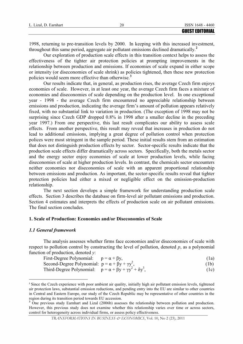
Equation (1b) permits an assessment of whether a firm faces economies ordiseconomies of scale but does not permit this assessment to depend on the level ofproduction. The second derivative with respect to production, denoted p", equals 2γ. A firmfaces economies of scale if p" < 0 and faces diseconomies of scale if p" > 0. If the quadraticparameter is negative (γ < 0), then a firm faces economies of scale regardless of theproduction level, as shown by Figure 1c. If the quadratic parameter is positive (γ > 0), then afirm faces economies of scale regardless of the production level, as shown by Figure 1d.

In contrast, equation (1c) permits an assessment of scale economies that depends onthe level of production. The second derivative with respect to production is p" = 2γ + 6δy.The quadratic and cubic production parameters, γ and δ, and the production level, y,collectively determine whether a firm faces economies or diseconomies of scale. If thequadratic parameter is negative (γ < 0) but the cubic parameter is positive (δ > 0), the sign ofp" and thus the production scale effect depends on the level of production. Figure 1ademonstrates that as production increases, a firm first faces economies of scale then laterdiseconomies of scale as p" shifts from negative to positive once production becomessufficiently high for the cubic term to dominate. If the quadratic parameter is positive (γ > 0)but the cubic parameter is negative (δ < 0), the sign of p" and the production scale effect againdepends on the level of production. Figure 1b demonstrates that as production increases, afirm first faces diseconomies of scale then later economies of scale. If both the quadratic andcubic production parameters are negative (γ < 0, δ < 0), then p" is unambiguously negativeand a firm faces economies of scale regardless of the production level, as shown in Figure 1c.If both parameters are positive (γ > 0, δ > 0), then p" is unambiguously positive and a firmfaces diseconomies of scale regardless of the production level, as shown in Figure 1d.

Figure 1 displays a variety of emission-production relationships. The main textdescribes the primary relationships shown in Figure 1. Figures 1c and Figure 1d also displayfour remaining possibilities that are relevant when either the quadratic or the cubic parameterequals zero (γ = 0 or δ = 0), which applies when either the estimated quadratic or cubicparameter is insignificantly different from zero. If the cubic term equals zero, then the third-degree polynomial becomes identical to the second-degree polynomial. Thus, the quadraticparameter (γ) alone dictates whether a firm faces economies or diseconomies of scale;consequently, the identified scale effect is independent of the production level. Figure 1cdisplays the case of economies of scale (γ < 0, δ=0), and Figure 1d displays the case ofdiseconomies of scale (γ > 0, δ = 0). If the quadratic term equals zero, then the cubicparameter (δ) alone dictates whether a firm faces economies or diseconomies of scale, and theidentified scale effect is independent of the production level. Figure 1c displays the case ofeconomies of scale (γ = 0, δ < 0); Figure 1d displays the case of diseconomies of scale (γ = 0,δ > 0).

This basic framework cleanly displays the possibilities of scale economies and scalediseconomies but does not explain the reasons for their existence. Given our empirical focus,we do not construct a formal theoretical model but instead draw upon the vast literature thatexamines returns to scale involving the standard relationship between output and inputs.



22

Notes: Y = Output P = Pollution

Source: the authors’ illustration.Figure 1. Economies and Diseconomies of Scale

This literature identifies two main forces: (1) an increased scale permits a greaterdivision of labour and a specialization of function, and (2) an increased scale entails some lossin efficiency because managerial oversight may become more complex (Nicholson, 1992).While not exhaustive, this short list facilitates our empirical objective.

For conceptual insight, we draw upon the vast literature that examines returns to scalein the standard context: identifying the relationship between output and inputs. Therelationship examined here is analogous to this standard relationship as long as we interpretpollution as the “output” of a “bad” (rather than a “good”) and “production of the good” as theinput into the generation of the “bad”. The analogy between output of a “good” and output ofa “bad” is obvious. The analogy between any standard input and “production of the good” isstraightforward if one views “production” as a “composite input,” i.e., production reflects theoutcome of combining multiple inputs.

Given this pair of analogies, we draw upon the related theoretical literature, startingwith Adam Smith’s seminal research on returns to scale and followed by classical theoreticalstudies, such as Douglas (1948), Stigler (1951), and Ferguson (1969). These theoreticalstudies identify two main forces affecting returns to scale. First, an increased scale permits agreater division of labour and a specialization of function (Nicholson, 1992). Second, anincreased scale entails some loss in efficiency because managerial oversight may becomemore complex (Nicholson, 1992). Put differently, the difficulties of managing a large-scaleoperation, especially maintaining good communication between managers and other workers,may eventually lead to decreases in the productivity of both labour and capital; for example,e.g., poor communication makes the workplace more impersonal, thus lowering morale



23

(Pindyck and Rubinfeld, 1989). Other forces affect returns to scale. As a positive force, alarger scale of operation may generate increasing returns to scale by allowing firms to exploitmore sophisticated, large-scale factories and equipment; as a negative force, a larger scale ofoperation may limit the entrepreneurial abilities of individual managers and other workers(Pindyck and Rubinfeld, 1989).

Consistent with these described forces, the standard depiction of returns to scalereveals economies of scale at lower levels of production, where the positive forces of divisionof labour and specialization dominate, yet this depiction reveals diseconomies of scale athigher levels of production, where the ever increasing difficulties of managing an unwieldyoperation dominate. This standard depiction is reflected in Figure 1a. Since pollutionrepresents a “bad” rather than a “good,” the curvature of Figure 1a is a mirror image of thecurvature from the standard depiction. However, this standard depiction may not hold in allcases. For example, some firms may never face any meaningful managerial difficulties thatare associated with larger scales of operation, at least within any relevant range, so economiesof scale may exist at all relevant production levels, as shown in Figure 1c. Lastly, neithereconomies nor diseconomies of scale may exist. According to Pindyck and Rubinfeld (1989,p.185), if no inputs are unique and all inputs are fully available as the scale of operationincreases, “...then constant returns to scale are guaranteed.”

With proper interpretation, this insight on returns to scale for the standard relationshipbetween output and inputs also applies to the relationship between pollution and production.First, the division of labour and specialization certainly applies to pollution control; as thescale of operations increases, employees are able to specialize in pollution control in generaland eventually air pollution control in particular. Second, only larger firms may be able tojustify the exploitation of more sophisticated, large-scale pollution abatement technologies.Third, a larger scale of operation may undermine managers’ abilities to communicatepollution control directives to workers. Fourth, larger firms may limit the scope ofentrepreneurial approaches to pollution control.

1.2 Transition economy of the Czech Republic

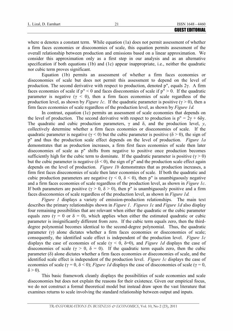
We utilize this basic framework to examine the effects of production scale on firm-level air pollutant emissions using data on Czech firms between 1993 and 1998, which is anideal time period for our study. First, the Czech Republic had a substantially degradedenvironment, especially poor ambient air quality, after the collapse of communism (WorldBank, 1992). In response to public concern, Czech government authorities took substantialand effective steps to decrease air emissions dramatically during the period 1991 to 1998(Czech Ministry of Environment, 1998). Specifically, the Czech government raised theemission charge rates imposed on the four air pollutants examined in this study and loweredthe permissible emission limits imposed on sources of the same air pollutants. Figure 2displays the downward trend of economy-wide air emissions over this period. A substantialdecline in economic activity in the early 1990s helps to explain part of this trend. In addition,firms pollution control efforts, such as the installation of electrostatic precipitators(“scrubbers”) and fuel switching, may also explain much of the displayed reduction in airpollution (World Bank, 1999).



24

Source: Czech Statistical Office, Czech Ministry of Environment, MZP (various years).

Figure 2. Air Pollutant Emissions in Czech Republic, 1990-2000

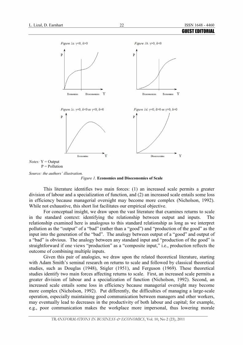
Second, consistent with this focus on pollution control efforts, investment inenvironmental protection was most important during the period between 1992 and 1998, asshown in Figure 3. As a percentage of the Czech gross domestic product (GDP), investmentrose dramatically after 1991 from a level of 1.3% to a peak of 2.5% in 1997 and tailed offafter 1998 back to a pre-transition level of 1.1% by 2000.

Source: Czech Statistical Office, Czech Ministry of Environment, MZP (various years).

Figure 3. Investment in Environmental Protection, 1990-2000

Third, the Czech Republic was attempting to enter the EU during this period and wasrequired to reduce its industrial emissions to qualify for membership.

These aspects of the Czech transition period prompt us to examine the possible effectsof tighter air protection policies on the relationship between production and pollution. Thetightening of Czech air protection policies most likely prompted Czech firms to lower their airpollutant emissions to some extent by investing in cleaner production technologies, betterabatement technologies, and/or environmental management systems. These investments mayhave influenced the relationship between production and pollution. In particular, one wouldhope that these investments expanded the range or intensity of scale economies. Based on ourbasic framework, we pose this empirical question: As air protection policies tightened andpolluting facilities were prompted to reduce their air pollutant emissions, were facilities moregreatly exploiting the division of labour and specialization and/or mitigating the efficiencyloss of complex oversight so that scale economies expanded in scope or intensity?

When answering this question, we do not attempt to identify the sources of any scaleeffects, e.g., complex management. In particular, we do not assess the various factorsaffecting a facility’s pollution level that are influenced by the level of production. Productionpresumably indirectly affects the pollution level by influencing a facility’s decisions



25

concerning its production technology [G(y)], input quality [Q(y)], and abatement effort[A(y)]. We could construct a more comprehensive pollution function that explicitlyincorporates these additional explanatory factors: p=f[y,G(y),Q(y),A(y)]. Instead, we chooseto telescope this more general relationship into the basic relationship: p=f(y). With thistelescoping in mind, the presence of economies (or diseconomies) of scale in pollution controlmay actually stem from economies (or diseconomies) of scale with respect to productiontechnology, input quality, and/or abatement effort. We do not attempt to identify the channelsconnecting these elements and pollution as our data does not allow it. Indeed, thisidentification is not necessary for our objective as we explore a highly reduced form ofemissions.

Given this perspective, we purposively exclude key explanatory factors, such asabatement effort. Thus, we are clearly not concerned about omitted variable bias. Rather thanclaiming that our analysis isolates the effect of production independent of other influences, weare claiming that the effect of production reflects all of the noted influences.

Consistent with our simplification regarding the emission-production relationship, wealso simplify the analysis connecting air protection policies to the emission-productionrelationship. Rather than examining the specific policies, we simply allow the emission-production relationship to vary over time as the protection policies tighten.

We do not analyze direct links relating tighter air protection policies to the emission-production relationship for two reasons. First, any conceptual analysis is complicated by themultiple dimensions that we funnel through the scale of operation as captured by theproduction level. In particular, the link between production and pollution stems from choicesmade regarding the use of production technologies, abatement technologies, environmentalmanagement systems, etc., and the noted policies most likely affected all of these choices, yetwe only analyze the outcome of these many choices. Thus, we do not attempt to deriveformally policy-related hypotheses.4

Second, empirical testing of any hypotheses derived for specific policies would bedifficult since tighter protection policies were applied simultaneously. On this point, weacknowledge that our analysis may not be able to irrefutably isolate the effect of tighter airprotection policies since other important elements were changing over this same time period.Nevertheless, we argue that protection policies are the primary element changing over thesample period with respect to the emission-production relationship.

Lastly, we argue that we are still able to assess scale economies and diseconomies inthe presence of air protection policies because the methods used to impose emission chargesand establish source-specific emission limits, in general, do not depend on production levels.Most obviously, emission charge rates do not depend on the level of production. Asimportant, the Czech environmental regulators established source-specific emissions limitsbased on either a concentration standard (e.g., milligrams of pollutant per liter of air) or a perproduction unit standard (e.g., tons of pollutant per ton of product) by scaling one of thesestandards according to the expected flow of air or production. Since neither standarddepended on the production level in nearly all cases, the established source-specific limitsreflected a proportional relationship between production and emissions.

4 Still, we could provide some indicative guidance when assessing possible effects of these policies. Forexample, escalating emission charge rates may have allowed smaller firms to justify the installation of moresophisticated abatement technologies. As another example, tighter effluent limits may have prompted firms todevelop an environmental management system that helps track compliance yet involves large fixed costs, whichcan be better amortized across a larger operational scale. This illustrative list is neither complete nor definitive.



26

2. Data on Emissions and Production

2.1 Panel data on emissions and production

To examine production at Czech firms, we gather data from a database provided by theprivate data vendor Aspekt. From this database, we gather balance sheet and income statementdata for the years 1993 to 1998, along with a firm’s primary sectoral classification. TheAspekt database includes all firms traded on either the primary or secondary market and amajority of the remaining large Czech firms. This comprehensive database has been used byprevious studies of Czech firm-level performance (Claessens and Djankov, 1999; Weiss andNikitin, 2002; Hanousek et al., 2007; Djankov, 1999). Production is measured as productionvalue in terms of Czech Crowns. To compare across the six years of the sample period, weadjust the production value using the Czech Consumer Price Index with 1998 as the base year.Our use of a fixed effects estimator (see Section 3.1) controls for any firm-specific variation inprices. As important, interactions with year indicators allow us to interpret production valuesas production quantity.

We also gather data on air pollutants emitted by Czech facilities during the years 1993and 1998. The included pollutants are carbon monoxide (CO), sulphur dioxide (SO2),particulate matter (PM), and nitrous oxides (NOx), which represent the main and most heavilyregulated pollutants in the Czech Republic, similar to other industrialized nations. The CzechHydrometeorological Institutes REZZO-1 database includes emissions for large, stationarysources at the unit level. The Institute aggregates emissions to the level of each facility beforepublicly releasing the data. We further aggregate emissions across all facilities associated witha single firm. Thus, the analysis links firm-level emissions data with other firm-level data,consistent with previous studies of firm-level environmental performance (Konar and Cohen,1997; Konar and Cohen, 2001; Earnhart and Lizal, 2006a; Khanna and Damon, 1999; Khannaet al., 1998; Arora and Cason, 1995; Arora and Cason, 1996). We add the four pollutants intoone composite measure of air emissions, similar to previous studies of environmentalperformance (Konar and Cohen, 1997; Konar and Cohen, 2001; Earnhart and Lizal, 2006a;Khanna and Damon, 1999; Khanna et al., 1998; Arora and Cason, 1995; Arora and Cason,1996).5

In order to generate the largest sample possible and to avoid a sample selection biasdue to attrition, we create an unbalanced panel of firm-year observations for the time period1993 to 1998. After merging the production data set and the air emissions data set, we screenfor meaningful data by applying the following criteria: non-missing emissions, positiveproduction value, positive total assets, and positive fixed assets. This merger and screeninggenerates an unbalanced panel of 2,632 observations from 631 firms.

2.2 Descriptive statistics

Table 1 summarizes emissions and production value. Table 2 disaggregates theemissions data by year. Consistent with the economy-wide statistics shown in Figure 2, overthe six years of the sample period, per-firm emissions declined. In 1993, the average firmemitted 1.287 tons of pollutants. Between 1993 and 1998, the mean value steadily andmonotonically declined. By 1998, the average value had dropped to 774 tons. The average

5 Preliminary analysis indicates that use of an alternative measure of emissions - an emission charge-weightedsum of air pollutant levels - generates reasonably similar estimation results.



27

firms emission intensity – emissions divided by production – also steadily and monotonicallydeclined over this period from a level of 0.70 to 0.42. These differences indicate that allowingthe functional relationship between emissions and production to vary over time is warranted.

Table 1. Statistical Summary of Production Value and Emissions

Variable Mean Std Dev Minimum MaximumProduction (000s CZK) a 1,618,320 4,618,679 1,869 89,906,018Emissions (tons) 962.1 4,059.9 0.0 48,883.0N = 2,632

Notes: a Production value is adjusted to 1998 real Czech Crowns (CZK) using the Czech CPI.Source: compiled by the authors.

Table 2. Year Distribution of Data and Year-Specific Descriptive Statistics for Emissions

Year # of Firms % ofSample

MeanEmissions(tons)

Mean Emission Intensity(tons/CZK)

1993 356 13.52 1,287 0.7041994 469 17.81 1,017 0.6571995 468 17.77 1,002 0.6401996 484 18.38 853 0.5711997 457 17.36 891 0.5241998 398 15.14 774 0.420

Source: compiled by authors.

Table 3. Sector-Specific Statistics for Emissions and Emission Intensity

Industry# ofObs

% ofObs

EmissionMean(tons)

EmissionIntensity(tons/CZK)

% of SampleEmissions

Agriculture, Hunting, Forestry, Fisheries 20 0.76 16.1 0.1202 0.01Mining and Quarrying 33 1.26 3,621.6 0.6431 4.72Manuf.: Food, Beverages, & Tobacco 397 15.11 150.2 0.1437 2.36Manuf.: Textiles, Textile Products, Leather, andLeather Products 216 8.22 265.5 0.3786 2.26

Manuf.: Wood, Wood Products, Pulp, Paper,Publishing & Printing 89 3.39 1,116.7 0.7255 3.92

Manuf.: Coke and Refined Petroleum 14 0.53 1,107.6 0.1028 0.61Manuf.: Chemicals, Chemical Products, andSynthetic Fibers 126 4.79 2,732.2 0.8245 13.59

Manuf.: Rubber and Plastic Products 53 2.02 92.9 0.1069 0.19Manuf.: Other Non-Metallic Minerals 234 8.90 542.3 0.4949 5.08Manuf.: Basic Metals, Fabricated Metal Products 308 11.72 1,702.5 0.6048 20.71Manuf.: Machinery & Equipment n.e.c. 301 11.45 165.6 0.1828 1.97Manuf.: Electrical and Optical Equipment 117 4.45 83.5 0.1357 0.39Manuf.: Transport Equipment 193 7.34 151.5 0.0553 1.16Manufacturing n.e.c. 92 3.50 144.8 0.2737 0.53Energy: Electricity & Natural Gas 160 6.09 6,677.0 2.6348 42.19Construction 120 4.57 42.0 0.0227 0.20Wholesale and Retail Trade; Motor VehicleRepair; Hotels and Restaurants; Transport, PostalService, Storage, & Telecommunicationa

50 1.91 17.8 0.0272 0.04

Finance, Real Estate, Rentals, Business, Research,Public Administration 73 2.74 14.4 0.0281 0.04

Education, Health, and Veterinary Services; OtherPublic and Social Services 33 1.26 27.1 0.1517 0.04

Notes: a These disparate sectors are combined because individually they represent too small a portion of the sample tofacilitate estimation. This sectoral category also includes 17 observations (0.65% of sample) from the sector of “Othern.e.c.”.Source: compiled by the authors.



28

Table 4. Mean Emissions and Emission Intensity by Individual Sector and Year

Sector Year Emissions Intensity Sector Year Emissions Intensity1993 267.00 0.367 1993 2,567.50 0.3491994 179.73 0.376 1994 1,703.22 0.3271995 142.56 0.240 1995 2,069.76 0.2651996 116.26 0.210 1996 1,672.78 0.2361997 119.41 0.188 1997 1,124.96 0.243

Food Products,Beverage,Tobacco

1998 113.98 0.211

Basic Metals,FabricatedMetal Products

1998 1,340.98 0.1321993 3,070.58 0.985 1993 402.52 0.7131994 2,786.67 1.008 1994 251.33 0.1761995 2,444.58 0.450 1995 83.85 0.1191996 1,794.10 0.502 1996 62.03 0.1141997 3,575.35 0.476 1997 54.97 0.439

Chemicals,ChemicalProducts,Synthetic Fibers

1998 2,653.87 0.399

TransportEquipment

1998 18.26 0.0501993 505.24 0.582 1993 13,609.60 5.7391994 585.47 0.494 1994 7,232.48 5.5841995 503.41 0.403 1995 6,761.53 5.7051996 463.39 0.336 1996 5,782.97 4.5901997 625.42 0.391 1997 6,026.41 4.579

Other Non-Metallic MineralProducts

1998 594.58 0.317

Energy

1998 4,151.59 3.465Source: compiled by the authors.

Table 3 displays the distribution of firms by industrial classification and demonstratesthat per-firm emissions and emission intensity differ dramatically across the variety of sectors.These differences seem to indicate that controlling for sectoral variation is important.

Table 4 distinguishes per-firm emissions and emission intensity by both year andsector, with a focus on key sectors. Certain sectors display a dramatic decline in emissionintensity over time, such as the transport equipment manufacturing sector, while other sectorsdisplay little variation in emission intensity over time, such as the non-metallic mineralproducts manufacturing sector. These differences seem to indicate that any consideration oftime variation in the emission-production relationship should be sensitive to sectoraldistinction.

3. Econometric Analysis of Air Pollutant Emission Levels

3.1 Econometric structure

In the econometric models, the dependent variable, pit denotes the amount of pollutionemitted by firm i in time period t. Emissions most likely depend strongly on the level ofproduction, denoted yit. Production enters in three terms: linear (yit), quadratic (yit

2), and cubic(yit

3). To control for variation over time, we include an indicator for each year between 1994and 1998, with 1993 as the benchmark, collectively denoted as vector Tt. To control forsector-specific variation, we generate an indicator for each sector displayed in Table 1.d,collectively denoted as vector Xi. Without additional manipulation, the fixed effects estimator,which is described below, subsumes the effects of sectoral indicators into its firm-specificfixed effects because the sector does not vary over time for a specific firm. For this reason, inthe first stage of analysis, we ignore the sectoral indicators. In the second stage, we fullyincorporate these sectoral indicators to the extent possible within the fixed effects estimator.

Given this notation, we formulate the following three polynomial (in production)econometric specifications:



29

1st-Degree: pit = αi + β yit + κ Tt’+ eit, (2a)2nd-Degree: pit = αi + β yit + γ yit

2 + κ Tt’+ eit, (2b)3rd-Degree: pit = αi + β yit + γ yit

2 + δ yit3 + κ Tt’+ eit, (2c)

where αi denotes the firm-specific intercept and eit denotes the error term.Production may be endogenous with respect to pollution. We address this concern in

three ways. First, we use Granger causality tests to demonstrate that production appears toGranger-cause emissions, yet emissions do not appear to Granger-cause production, i.e., theGranger causality test statistics reject the null hypothesis of zero influence in the former casebut cannot safely reject the null hypothesis of zero influence in the latter case.

When testing for Granger causality, we consistently use two lags of the variable whosecausality is being assessed while varying the number of lags - one or two - in the controlvariable. Regardless of the specification of the time lag for the control variable, we find thatemissions never Granger-cause production. The p-values for these Granger test statistics areabove 0.95, strongly indicating the lack of any relationship. Moreover, the p-values for theindividual coefficients are nearly as high; they are above 0.80. On the other hand, productioncan Granger-cause emissions. The individual lag coefficients on production are significant forboth specifications; they are even close to the 5% significance level for the one-lagspecification, with p-values of 0.051 and 0.053. The p-values for the joint tests indicatesignificance levels that are quite close to the 10% critical threshold; the p-value equals 0.102and 0.149 for the one-lag specification and two-lag specification, respectively.

We employ a fixed effects estimator to generate these Granger causality test statistics.Consequently, we must address the fact that the presence of lagged values of the dependentvariable on the right-hand side of the equations used to test the Granger causality in a dynamicpanel data framework can lead to inconsistent parameter estimates unless the time dimensionof the panel is very large (Nerlove, 1967; Nickell, 1981; Keane and Runkle, 1992). Andersonand Hsiao (1981) propose using twice-lagged levels of the right-hand side variables asinstruments. Kiviet (1995) establishes the superiority of using twice-lagged levels over laggeddifferences and suggests an alternative approach that involves direct calculation of biases andcorrection of the least squares estimates. Simulation results in Judson and Owen (1999) showthat Anderson-Hsiao estimators, while the least biased among the available alternatives, areconsiderably less efficient than the alternative proposed by Kiviet (1995). Fortunately,simulation results by Judson and Owen (1999, p.13) also show that the bias problems arealmost entirely concentrated in the coefficient of the lagged dependent variables, while biasesin the coefficients of independent variables, which are the variables important for the test, arerelatively small and cannot be used to distinguish between estimators [including OLS]. Insum, we elect to ignore the bias corrections in the Granger-causality tests for the followingreasons. First, we are not interested in point estimates of the noted coefficients. Second, anycorrection for biases would result in a significant loss of efficiency that would damage ourability to assess the causal relationships. Third, the coefficient bias is most likely small.Fourth, the unbalanced panel nature of the data greatly complicates the bias correctionprovided by Kiviet (1995).

Thus, with some confidence, while acknowledging that we possess only a very shorttime span for testing, we can eliminate any concern about a simultaneous determination ofproduction and pollution and focus our concern on the endogeneity of production.6 Second,previous studies of environmental performance also incorporate a contemporaneous measure

6 The test statistics and associated conclusions are consistent with the nature of pollution as a byproduct ofproduction.



30

of production as an explanatory factor, implicitly treating production as pre-determined withrespect to pollution (Mickwitz, 2003; Foulon et al., 2002; Bluffstone, 1999; Khanna andDamon, 1999; Magat and Viscusi, 1990). Third and most important, we implement theHausman test for exogeneity (Wooldridge, 2002). The Hausman test statistic fails to reject thenull hypothesis of exogeneity in each specification.7

To accommodate the panel data structure, we estimate equations (2a), (2b), and (2c)using a fixed effects estimator since it dominates the other standard panel estimators: pooledOLS and random effects. Results from a set of F-tests of fixed effects, which are reported inTable 5, indicate that pooled OLS suffers from omitted variable bias due to excluding firm-specific intercept terms.

Table 5. Exclusion of Interactions between Year Indicators and Production Terms

RHS Variable1st-DegreePolynomial

2nd-DegreePolynomial

3rd-DegreePolynomial

Production a0.123(0.028)

*** 0.435(0.055)

*** 0.505(0.084)

***

Production-squared a N/A- 3.56 E-6(0.54 E-6)

*** - 6.44 E-6(2.62 E-6)

***

Production-cubed a N/A N/A2.28 E-11(2.03 E-11)

1994 b- 265.66(106.70)

*** - 218.62(105.80)

** - 215.26(105.80)

**

1995 b- 336.05(107.60)

*** - 285.37(106.70)

*** - 281.18(106.80)

***

1996 b- 463.53(107.60)

*** - 378.86(107.30)

*** - 371.02(107.50)

***

1997 b- 585.91(109.10)

*** - 477.68(109.20)

*** - 469.17(109.50)

***

1998 b- 778.64(113.60)

*** - 647.08(114.20)

*** - 634.64(114.70)

***

Adjusted R2 0.908 0.911 0.910F-test of Individual Effects [significance level]

29.79[0.0000]

26.43[0.0000]

26.29[0.0000]

Hausman FE vs. RE c

[significance level]27.63[0.0003]

26.71[0.0004]

24.76[0.0017]

No. of Firms / No. of Obs 630 / 2,626 630 / 2,626 630 / 2,626Notes: Standard errors are noted inside parentheses; p-values are noted inside square brackets.

*, **, and *** indicate statistical significance at the 10%, 5%, and 1% levels, respectively.Each regression also includes 630 firm-specific indicators.a Units for production are millions of Czech crowns; units for production-squared are trillions of Czech

crowns; units for production-cubed are quintillions of Czech crowns.b Omitted category is 1993.c Estimation of the random effects model includes 19 sector-specific indicators while restricting the sum

of these indicators= coefficients to zero.

Source: compiled by the authors.

7 The test statistics are 1.01, 0.22, and 0.25, respectively, for equations (2a), (2b), and (2c); p-values are 0.32,0.83, and 0.80. To generate these Hausman test statistics, we use several instruments for production: linear,quadratic, and cubic terms for preceding stock levels, equity, total assets, short-term and long-term liabilities,and short-term and long-term bank loans, along with the fixed to total assets ratio, depreciation to fixed assetsratio, and intangible to tangible fixed assets ratio. The failure to reject the null hypothesis of exogeneity is robustto the selection of instruments.



31

Results from a set of Hausman tests of random effects, which are shown in Table 5,indicate that the random effects estimates are inconsistent in all cases. In contrast, fixedeffects estimates are consistent by design. The fixed effects estimator controls forheterogeneity across individual firms.

We allow the functional relationship between emissions and production to vary overtime by interacting each of the three production terms - yit, yit

2, and yit3 - with each of the five

year-specific indicators - T94, T95, T96, T97, and T98. Then we insert the interactive terms intoequations (2a), (2b), and (2c). For example, after inserting the interactive terms into the third-degree polynomial, the regression equation becomes the following:

pit = αi + β yit + γ yit2 + δ yit

3 + κ Tt’ + Γ [yitTt’]+ Θ [yit2Tt’]+ ξ [yit

3Tt’]+ eit . (3)This standard fixed effects model indirectly estimates the coefficients associated with

the vector of sectoral indicators, Xj, since each sector-specific coefficient equals the averagevalue of the firm-specific intercept coefficients associated with a particular sector. Thus, thefirst step of analysis controls for sectoral variation by allowing the emissions-productioncurve to shift up or down.

As the second step, we extend this consideration of sectoral variation by modifying thefixed effects estimator. First, we interact the sectoral indicators with each of the threeproduction terms. By utilizing the full set of sectoral indicators, the analysis generates acoefficient set for each sector. Fixed effects estimation of each sector-specific sub-sampleseparately generates coefficient magnitudes that are identical to those reported here; however,the chosen approach improves the efficiency of the estimates, i.e., lower standard errors (andconsiderably so). By incorporating the sectoral interactions, the relationship betweenemissions and production is more uniform across firms because they operate in the samesector, thus, possessing similar production and abatement technologies and utilizingcomparable production and pollution management methods.

Second, the analysis interacts each of the sector-specific production terms with the setof year indicators. This approach allows the emission-production relationship to vary overtime and across sectors; i.e., this approach permits technological change to alter theproduction scale effects and to impact various sectors to a different degree and at a differentpace.

Third, the analysis interacts the sectoral indicators with the year indicators, whichallows year-specific intercepts to vary across sectors. Given the construction of the fixedeffects estimator, no general intercept term exists. Instead, the model includes only a set offirm-specific intercepts. Thus, the year-specific intercepts represent temporal adjustments tothe firm-specific intercepts that apply to all firms uniformly. By interacting the year-specificintercepts with the sectoral indicators, the analysis allows the firm-specific intercepts to adjustover time in a manner consistent with the sector of the specific firm. With properinterpretation, this accommodation implies that changes in the regulatory climate may alterthe connections between firm-specific, time-invariant features and air pollution control in amanner consistent with the relevant sector rather than all sectors in general.

Based on the estimation results involving the metals sector, independent of theemission-production relationship, emissions fell over time, in general, as shown by the year-specific intercepts, with 1995 as the exception. Relative to 1993, emissions are significantlylower in 1997 and 1998 (p=0.018, 0.005). The decline between 1996 and 1997 is alsosignificant (p=0.013). This overall decline seems to indicate that by the end of the transitionperiod Czech firms in the metals sector had lowered their pollution in ways not related toproduction scale effects. Based on the estimation results involving the energy sector,independent of the emission-production relationship, as shown by year-specific intercepts,



32

emissions are comparable to their 1993 level with the exception of 1997, which issignificantly lower (p=0.01). Nevertheless, these same intercepts indicate significant year-to-year differences - up, down, up - between the years 1995 to 1998 (p=0.10, 0.0002, 0.005).These differences indicate that the energy firms’ control of air pollution in ways not related toproduction scale effects does not appear sensitive to the progression of the Czech transition.

After generating these interaction terms, we insert them into equations (2a), (2b), and(2c). For example, after inserting the interaction terms into the first-degree polynomial, theregression equation becomes the following:

pit = αi + β [yitXj’] + κ [Tt’Xj’] + Γ [yitTt’Xj’] + eit . (4)This second analytical approach generates estimation results for each separate sector.

A full evaluation and assessment of the results for all 19 sectors shown in Table 4 seemsunwarranted. Instead, we focus on a smaller subset of five important sectors:

(1) Manufacturing of Food Products, Beverages, and Tobacco (“foods”);(2) Manufacturing of Chemicals, Chemical Products, and Synthetic Fibers

(“chemicals”);(3) Manufacturing of Basic Metals and Fabricated Metal Products (“metals”);(4) Manufacturing of Transport Equipment; and(5) Energy: Electricity and Natural Gas (“energy”).Three sectors represent heavy polluters since they rank as the three largest Czech

sectors in terms of air pollution. The energy sector contributes an amazing 42% of all sample-wide emissions, the metals sector contributes 21%, and the chemicals sector contributes 14%(see Table 4). Collectively, these three sectors contribute an astounding 77% of sample-wideemissions. Similarly, the average firms in these three sectors emit air pollutants at levels farabove the sample average of 962 tons per year. The average energy firm emits 6,677 tons Balmost seven times the sample average; the average chemicals firm emits 2,732 tons, almostthree times the sample average. The average metals firm emits 1,703 tons. As important, thesethree sectors invested heavily into environmental protection efforts during the sample period(Czech Ministry of Environment, 1999). The energy sector alone represented almost 50% ofall air-related environmental investment during the 1994 to 1999 period (Brůha et al., 2005).

To complement these three heavy polluting sectors, we add two relatively lightpolluting sectors. The foods sector and the transport equipment sector contribute only 2% and1% of sample-wide emissions, respectively, while their average firms emit only 150 and 152tons per year, respectively, as shown in Table 4. In addition, the foods sector is large; itcontains the most firms of any sector: 15% of the sample.

In contrast to the positive reasons for selecting the chosen five sectors, negativereasons exist for purposively choosing not to examine the other 14 sectors.

First, we purposefully avoid excessively light polluting sectors mostly because ouranalysis requires sufficient variation in the dependent variable. For example, the averageconstruction firm emits only 42 tons, less than 5% of the sample average of 962 tons. Inaddition, these light polluting sectors appear too “clean” to warrant consideration, at least forthe purposes of policy analysis.

Second, we avoid disparate sectors. Certain sectors are simply too disparate togenerate any meaningful analysis of the particular group of firms; the manufacturing n.e.c.sector represents the most extreme example. Disparate sectors belie the claim that sectoraldistinction helps the analysis to better capture the emission-production relationship givengreater uniformity across the examined firms. (The last three sectors shown in Table 4arguably represent the most disparate sectors in our sample. Given the small sample sizes ofthese sectors, we combined these already disparate sectors into an even more disparate, but



33

sufficiently large, set of firms for the purposes of estimation.) Consequently, we do notevaluate disparate sectors. Nevertheless, our initial analysis examined two moderatelydisparate sectors: the machinery and equipment n.e.c. manufacturing sector (hereafter“machinery and equipment sector”) and the non-metallic minerals manufacturing sector(hereafter “non-metallic minerals sector”). We examined these two particular moderately-disparate sectors because their large sample sizes permitted us to demonstrate with someconfidence the otherwise assumed claim that sufficient disparity undermines the ability toconnect emissions and production. We utilized both sectors for this one purpose in order toassess the robustness of the demonstration: the machinery and equipment sector is a relativelylight polluter, with an average annual emission level of 166 tons per firm, while the non-metallic minerals sector is a relatively moderate polluter, with an average annual emissionlevel of 542 tons. Consistent with our claim that the dimension of disparity is important forthe analysis, our initial analysis demonstrates that we are not able to estimate a statisticallysignificant relationship between emissions and production for either moderately disparatesector.

Third, we do not assess three particular sectors:(1) agriculture, hunting, forestry, fisheries;(2) mining and quarrying; and(3) manufacturing of coke and refined petroleum due to their tiny sample sizes, which

are shown in Table 4.The loss of the first sector need not undermine the policy relevance of our analysis

since the average firm in this sector emits a relatively very small amount (16 tons, as opposedto the sample average of 962 tons) and contributes only 0.01% of all emissions in our sample,as shown in Table 4. The loss of the other two sectors at first may potentially undermine thestudy’s policy relevance since the average firm in these two sectors emits very large amountsof pollutants, especially in the mining and quarrying sector. Fortunately, the small samplesizes for these two sectors also imply that policymakers are able to address the firms in thesesectors on a case-by-case basis rather than relying on any study of sectors. The mining andquarrying sector and the coke and refined petroleum manufacturing sector contain only 8 and3 firms, respectively. Rather than allowing these three sectors to undermine the efficiencygains from our regression approach, we delete the firms in these sectors from our sample.Regardless of our interest in the remaining sectors, the analysis retains all of the other sectorsin some useful form since their sample sizes permit at least reasonable accommodation in theregression system.

Fourth, we do not evaluate certain sectors for a combination of reasons argued above.For example, we do not evaluate the manufacturing of wood, wood products, pulp, paper,paper products, and publishing and printing sector. This sector includes somewhat disparatesub-sectors, as evidenced by previous studies’ focus on only pulp and paper manufacturingfacilities (e.g., Nadeau, 1997). A sample size of 89 observations is sufficiently small toconstrain our analytical ability to investigate variation in the production term effects over timewithout exhausting the degrees of freedom, especially in the third-degree polynomialspecification.

We employ the two described analytical approaches to generate estimation results,which we examine in the subsequent sub-section.



34

3.2 Estimation results

3.2.1 Fixed effects estimates: without sectoral distinctions

First, we consider the standard fixed effects estimates with and without interactionsbetween the production terms and the year indicators. Results from the specifications lackingthese interactions are shown in Table 5. Results from the three polynomial specifications areboth qualitatively and quantitatively very similar. Consequently, we interpret them as a whole.Based on the estimated year indicators, relative to 1993, emissions are lower in every singlesubsequent year. Moreover, the difference grows monotonically over time. Just as important,emissions are significantly rising in production, as indicated by the linear production term.Based on the first-degree polynomial, each additional one million Czech Crown increase inproduction value leads to an increase of 0.12 tons of air pollution. By including the quadraticproduction term, the effect rises to 0.44 tons; by additionally including the cubic productionterm, the effect rises further to 0.51. The quadratic production effect is significantly negativein both relevant polynomial specifications. The cubic production term does not significantlyaffect emissions. Collectively, these results indicate that emissions are generally rising inproduction but at a declining rate regardless of the production level.

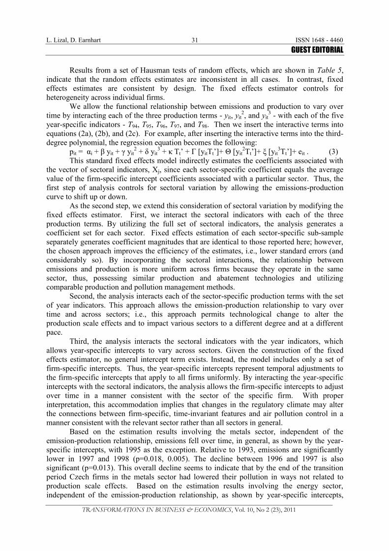
Next, consider the results from the specifications that contain interactions betweenyear indicators and the production terms, as shown in Table 6. Rather than tabulating theproduction-related coefficient estimates for the base year of 1993 and the interactionsinvolving the five-year indicators, we display the year-specific production-related coefficients,which represent a simple sum of the base-year coefficients and the relevant year interactioncoefficients, e.g., “1994 linear production” coefficient = [“1993 linear production”coefficient] + [“1994 indicator × linear production coefficient”]. (Reported p-values areconsistent with the calculated sum of the two coefficient estimates.) We assess the estimationresults of the three specifications as a whole.

First, we identify general tendencies. The results for the linear production coefficientsin general do not differ across the three specifications. With the exception of 1998, the linearproduction effect is significantly positive for each year. The quadratic production terms in thesecond-degree polynomial specification are significantly negative in every year except 1998.The cubic production terms are negative in all but one year and significantly so in three years;in the exceptional year of 1997, the cubic term is significantly positive.

Second, we utilize the year-specific coefficients to generate year-specific conclusions.We focus on the highest-order specification with a significant corresponding term unless alower-order term is questionable. For 1993, the cubic production term is not significant in thethird-degree polynomial. For both 1994 and 1996, the cubic production term is significant butthe quadratic production term is insignificantly positive in the third-degree polynomial yetsignificantly negative in the second-degree polynomial. Based on this pattern, we concludethat the second-degree polynomial dominates the third-degree polynomial for 1993, 1994, and1996. Thus, emissions are generally rising in production but at a declining rate regardless ofthe production level so that firms enjoy economies of scale regardless of the production level(see Figure 1c).

For 1995, the best specification is not obvious. Estimates from the third-degreepolynomial reveal that the quadratic production effect is significantly positive while the cubicproduction effect is significantly negative. However, they also indicate that the linearproduction effect is insignificantly positive (p=0.47). If we focus on the cubic term, we selectthe third-degree polynomial and generate this conclusion: as production rises in 1995, firms



35

first face diseconomies of scale but later enjoy economies of scale (see Figure 1b). However,if we focus on the linear term, we select the second-degree polynomial and generate aconclusion identical to those for 1993, 1994, and 1996. For consistency with the surroundingyears, we select the second-degree polynomial.

Table 6. Inclusion of Interactions between Year Indicators and Production Terms

1st-DegreePolynomial 2nd-Degree Polynomial 3rd-Degree Polynomial

Regressor Year Effect p-value Effect p-value Effect p-value1993 0.1914 0.0001 0.4584 0.0001 0.5423 0.00011994 0.1610 0.0001 0.4994 0.0001 0.3479 0.00741995 0.2102 0.0001 0.4860 0.0001 0.0832 0.46851996 0.1456 0.0001 0.3421 0.0001 0.2014 0.08251997 0.0522 0.0765 0.0314 0.6478 0.2266 0.0322

LinearProductionTerms a

1998 - 0.0669 0.1598 - 0.0221 0.8168 - 0.0566 0.70921993 N/A N/A - 8.18 E-6 0.0001 - 8.55 E-6 0.09911994 N/A N/A - 13.7 E-6 0.0001 13.37 E-6 0.19581995 N/A N/A - 10.5 E-6 0.0001 32.96 E-6 0.00011996 N/A N/A - 6.98 E-6 0.0001 6.56 E-6 0.32221997 N/A N/A - 1.23 E-6 0.0825 - 11.97 E-6 0.0122

QuadraticProductionTerms a

1998 N/A N/A - 3.60 E-6 0.2146 3.84 E-6 0.78971993 N/A N/A N/A N/A - 0.08 E-9 0.21671994 N/A N/A N/A N/A - 0.73 E-9 0.00081995 N/A N/A N/A N/A - 0.85 E-9 0.00011996 N/A N/A N/A N/A - 0.26 E-9 0.00191997 N/A N/A N/A N/A 0.07 E-9 0.0851

CubicProductionTerms a

1998 N/A N/A N/A N/A - 0.28 E-9 0.37681994 - 172.24 0.1210 - 169.48 0.1779 40.09 0.77131995 - 317.94 0.0045 - 261.66 0.0372 155.70 0.25341996 - 342.03 0.0021 - 202.28 0.1050 29.14 0.82921997 - 313.53 0.0054 53.13 0.6742 16.36 0.9047

Year-SpecificIntercepts b

1998 - 371.41 0.0017 - 63.87 0.6349 71.36 0.6240Adjusted R2 0.9142 0.9174 0.9208F-test: Fixed Effects [significance level]

31.14[0.0001]

28.42[0.0001]

28.20[0.0001]

N of Firms/N of Obs 630 / 2,626 630 / 2,626 630 / 2,626Notes : Year-Specific Production Terms equal Sum of Base-Year Effects and Year Interactive Terms.

Standard errors are noted inside parentheses; p-values are noted inside square brackets.*, **, and *** indicate statistical significance at the 10%, 5%, and 1% levels, respectively.Each regression also includes an intercept term, in addition to 630 firm-specific indicators.a Units for production are millions of Czech crowns; units for production-squared are trillions of Czech

crowns; units for production-cubed are quintillions of Czech crowns.b Omitted category is 1993.

Source: compiled by the authors.

The 1997 estimates (based on the third-degree polynomial) indicate that, as productionrises, firms first enjoy economies of scale, while later facing diseconomies of scale (seeFigure 1a).

The 1998 estimates indicate that no significant relationship exists between productionand emissions according to any dimension: linear, quadratic, or cubic.

In sum, results from the standard fixed effects estimation that includes year-productioninteractions indicate that the third-degree polynomial is either unwarranted or problematic for



36

five of the six years. This higher-order polynomial appears warranted only for 1997. For theother years, except 1998, the second-degree polynomial results indicate that firms faceeconomies of scale regardless of the production level; the same conclusion is based on theresults from the specifications lacking year-production interactions. In 1998, firms faced noappreciable increase in emissions as production rose. Thus, the inclusion of year-productioninteractions helps us to better classify the years 1997 and 1998.

3.2.2. Fixed effects estimates: with sectoral distinctions

As the second analytical approach, we assess the estimation results generated byeconometric specifications that interact sectoral indicators with year-specific production termsand year indicators. Results for the selected sectors are shown in Tables below. Rather thanreporting all of the polynomial specifications for all five sectors of interest, we report for eachsector only the “best” specification, as based on the significance of the production terms (e.g.,if the linear production term is significant in only the first-degree polynomial, yet thequadratic and cubic terms are insignificant in the higher-order polynomials, then the first-degree polynomial is “best”).

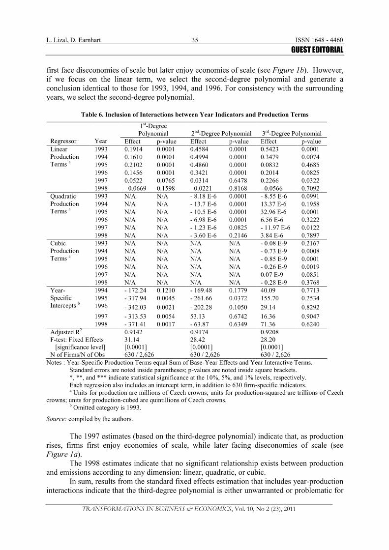
First, we assess the metals sector, for which the third-degree polynomial is “best.” Asshown in Table 7, in every year, the linear production term is significantly positive, thequadratic production term is significantly negative, and the cubic term is significantlypositive. Thus, regardless of the point in the Czech economic transition, the metals sectorenjoys economies of scale at lower production levels, while it faces diseconomies of scale athigher production levels.

Yet, the quantitative nature of this emission-production relationship is changing overtime. In general, the relationship is getting steeper and more curved, with stronger economiesof scale in the lower production levels but stronger diseconomies of scale in the upperproduction levels. (In all three dimensions, 1995 represents an exception to the overallprogression.) The linear production effect rises over time. Relative to 1993, the effect issignificantly greater in 1997 and 1998 (p=0.0001). Moreover, starting from 1995, the effectrises monotonically through 1998, (significantly between each pair of years [p=0.001, 0.0001,0.072]). In contrast, the quadratic production effect becomes more negative over time,indicating stronger economies of scale. Relative to 1993, the effect is significantly morenegative in 1996, 1997, and 1998 (p=0.0001). Moreover, starting from 1995, the effect dropsmonotonically through 1998 (significantly between each pair of years [p=0.0001]). Yet, thecubic production effect rises over time too, indicating stronger diseconomies of scale.Relative to the initial year of 1993, the effect is significantly greater in 1996, 1997, and 1998(p=0.08, 0.0001, 0.0001). And starting from 1995, the effect rises monotonically through1998 (significantly between each pair of years [p=0.0001]).

Second, we assess the energy sector, for which the third-degree polynomial is Abest.@As shown in Table 7, the linear production term is significantly positive in every year, thoughthe p-values for 1996 and 1998 are highly marginal at levels of 0.14 and 0.13, respectively.The quadratic production term is significantly negative and the cubic term is significantlypositive in every year. Thus, regardless of the point in the Czech economic transition, theenergy sector enjoys economies of scale at lower production levels, while facingdiseconomies of scale at higher production levels, similar to the metals sectors.



37

Table 7. Metals Sector and Energy Sector

Metals Sector (N=308) Energy Sector (N=160)Regressor Year Coefficient p-value Coefficient p-value

1993 1.038 0.0034 4.58 0.01341994 1.099 0.0046 4.97 0.01481995 0.669 0.0579 5.05 0.02071996 1.273 0.0034 3.39 0.14461997 2.500 0.0001 9.74 0.0001

LinearProductionTerms

1998 2.855 0.0001 4.21 0.13011993 - 0.2304 E-3 0.0001 -2.083 E-3 0.00061994 - 0.2710 E-3 0.0001 - 4.022 0.00011995 - 0.1678 E-3 0.0001 - 4.535 0.00011996 - 0.3483 E-3 0.0001 - 4.953 0.00011997 - 0.6253 E-3 0.0001 - 9.036 0.0001

QuadraticProductionTerms

1998 - 0.7048 E-3 0.0001 - 8.851 0.00011993 2.848 E-9 0.0001 120.83 E-9 0.01891994 3.343 E-9 0.0001 379.27 E-9 0.00011995 0.904 E-9 0.1737 464.28 E-9 0.00011996 4.327 E-9 0.0001 568.34 E-9 0.00011997 11.957 E-9 0.0001 1,108.1 E-9 0.0001

CubicProductionTerms

1998 14.106 E-9 0.0001 1,282.1 E-9 0.00011994 - 122.35 0.6989 - 553.91 0.45441995 84.10 0.7905 - 743.18 0.30541996 - 205.12 0.5204 15.16 0.98361997 - 755.30 0.0180 - 1,933.21 0.0120

Year-SpecificIntercepts a

1998 - 918.18 0.0051 - 352.67 0.6538System Adjusted R2 0.9704F-test: Fixed Effects [significance level]

16.83[0.0001]

N of Firms/N of Obs 611 / 2,560Notes: a 1993 is the benchmark year.Source: compiled by the authors.

Table 8. Sectors: Chemicals; Foods, Beverages, & Tobacco; Transport Equipment

Chemicals Sector(N=126)

Foods, Beverages, &Tobacco Sector (N=397)

Transport EquipmentSector (N=193)

Regressor Year Coeff. p-value Coeff. p-value Coeff. p-value1993 0.4675 0.0001 0.0302 0.9006 0.2120 0.21931994 0.4714 0.0001 0.0358 0.8812 0.2931 0.25741995 0.4357 0.0001 0.0482 0.8389 0.1762 0.41631996 0.3643 0.0410 0.0255 0.9159 0.1467 0.41451997 0.5225 0.0030 0.0347 0.8487 0.1021 0.4100

LinearProductionTerms

1998 - 0.1025 0.6011 0.0434 0.8465 0.1310 0.62591994 100.98 0.8381 - 73.74 0.7942 - 125.06 0.69111995 - 313.17 0.5310 - 130.68 0.6473 - 100.31 0.75511996 - 187.95 0.7299 - 129.70 0.6466 - 104.71 0.74341997 - 697.83 0.2026 - 152.44 0.6037 - 79.03 0.8113

Year-SpecificIntercepts a

1998 621.44 0.2609 - 181.09 0.5440 - 100.11 0.8013System Adjusted R2 0.9704F-test: Fixed Effects [significance level]

16.83[0.0001]

N of Firms/N of Obs 611 / 2,560Notes: a 1993 is the benchmark year.Source: compiled by the authors.



38

Yet, the quantitative nature of this emission-production relationship is changing overtime, as with the metals sector. In general, the relationship is more curved, with strongereconomies of scale in the lower production levels but stronger diseconomies of scale in theupper production levels. In general, the linear production effect does not vary over time fromits initial 1993 level, with an exceptionally stronger effect in 1997 [p=0.0002]. (Nevertheless,this effect significantly varies between the years 1995 to 1998 [p=0.10, 0.0001, 0.0001].) Incontrast, the quadratic production effect becomes more negative over time, indicating strongereconomies of scale. Relative to 1993, the effect is significantly more negative in every otheryear (p=0.0001). Moreover, starting from 1993, the effect drops monotonically through 1997,while leveling off in 1998. [Only the drops between 1993 and 1994 and between 1996 and1997 prove significant (p=0.0001).] Yet, the cubic production effect rises over time too,indicating stronger diseconomies of scale. Relative to 1993, the effect is significantly greaterin every other year (p=0.0001) and rises monotonically through 1998 (significantly betweeneach pair of years [p=0.0001, 0.07, 0.06, 0.0001, 0.04]).

Since the metals sector and energy sector possess a similar emission-productionrelationship, we compare those using F-tests of equal effects. For this comparison, weorganize the differences in three ways: (#1) we assess separately each dimension - linear,quadratic, cubic - jointly for all years, (#2) we assess the dimensions jointly for each singleyear, and (#3) we assess the individual dimensions separately for each year. Whenconsidering the year-specific effects jointly (#1), the two sectors are clearly different in allthree dimensions (p=0.0001). Similarly, when considering the production effects jointly (#2),the two sectors are clearly different in every year (p=0.0001). Specifically, each of theproduction effects linear, quadratic, and cubic is stronger for the energy sector than the metalssector in every year (#3); note that the quadratic production effect is “stronger” when it ismore negative. All of these differences are significant except the linear production effect in1996 and 1998. These two exceptions aside, in every year, the energy sector faces a steeperbut more curved emission-production relationship.

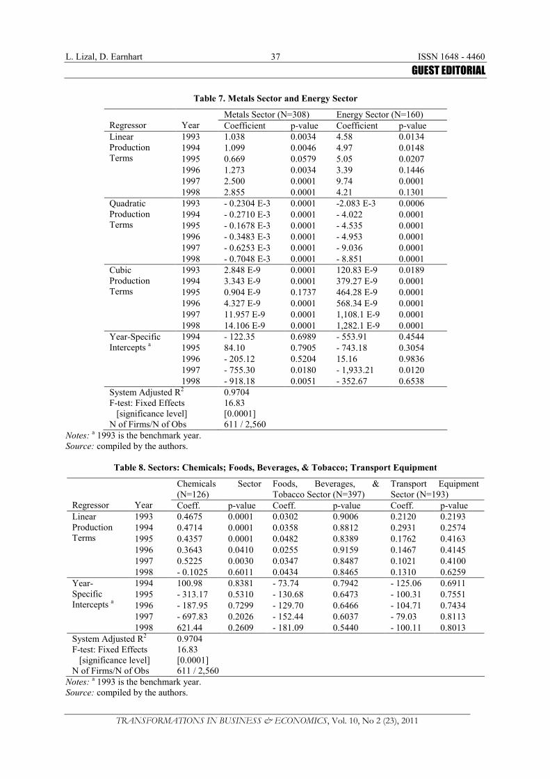
Third, we assess the chemical sector, for which the first-degree polynomial is “best.”(In the second-degree polynomial, only the linear production term proves significant. In thethird-degree polynomial, none of the production terms prove significant.) As shown in Table8, the linear production term significantly and positively affects emissions in every yearbetween 1993 and 1997. However, in 1998, this effect significantly drops from its 1993 level(p=0.001) and becomes insignificantly different from zero.8 Otherwise, the linear productioneffect does not vary over time. These results indicate that the chemicals sector encountersneither economies nor diseconomies of scale with a mostly stable, proportional relationshipbetween emissions and production.9

Fourth, we assess the foods sector and transport equipment sector, which bothrepresent relatively “clean” sectors. Consistent with this depiction, results for both sectorsstrongly indicate that emissions are not a function of production in any dimension regardlessof the polynomial specification.10 (Results for the first-degree polynomials are shown in Table

8 While insignificant, the coefficient magnitude drops so much in 1998 that it becomes negative despite theremoval of a single “influential” observation. When constraining the linear production effect to be equal overtime, the estimated coefficient is significantly positive (p=0.0001). Thus, the 1998 effect represents theexception, especially since it represents the only year of economic recession in the sample period.9 The year-specific intercepts reveal a stable control of emissions in ways not related to production scale effectson the part of individual chemical firms.10 Firms in these sectors may be generating emissions typically from combustion for heating. If true, the level ofemissions depends on important factors, such as the degree of insulation in facility buildings that need not berelated to production levels.



39

8) For both sectors, this conclusion is fully robust to the restriction of the production termsbeing equal over time, which cannot be rejected based on F-tests.

3.3 Interpretation of estimation results

The standard fixed effects estimates support the following conclusions. As productionrises, the average Czech firm enjoys economies of scale in general and for most of the specificyears. Estimates indicate that firms in 1993, 1994, 1995, and 1996 enjoy economies of scaleregardless of the production level. As an extension, the standard estimates indicate that firmsin 1997 also enjoy economies of scale, but only initially; at sufficiently high productionlevels, firms face diseconomies of scale. The results for 1998, a more exceptional year,indicate no discernable connection between emissions and production. These results indicatethat tighter air protection policies did not expand Czech firms’ enjoyment of scale economies.On the contrary, these results in general reveal that tighter policies seem to restrict the scopeof scale economies. Results for 1998 are difficult to interpret since they do not permit anassessment of scale effects. However, from another perspective, these results may reveal thatwhen protection policies were most stringent, Czech firms were able to increase theirproduction without any appreciable increase in emissions, implying that tighter policies werequite successful.

We next interpret the results when the analysis allows the emission-productionrelationship to vary across sectors, with a focus on the three largest air polluting Czechsectors: metals, energy, and chemicals. The sector-specific results support these conclusions.First, the production scale effects differ dramatically across sectors. Second, both the metalssector and the energy sector enjoy economies of scale at lower production levels, while facingdiseconomies of scale at higher production levels. In contrast, the chemicals sectorencounters neither economies nor diseconomies of scale with an apparent proportionalrelationship between emissions and production. Third, depending on the sector, the emission-production relationship varies over time as air protection policies tightened. For both themetals and energy sectors, economies of scale at lower production levels intensified yet,diseconomies of scale at higher production levels also intensified. Thus, the effect of tighterpolicies is clearly mixed. In contrast, for the chemicals sector, the effect of tighter protectionpolicies is negligible, as shown by the stable emission-production relationship over time. Theremaining sectors are too difficult to assess since no meaningful emission-productionrelationship exists in any year.

4. Additional Policy Implications

This final section draws additional policy implications, conditional on the imposition ofsource-specific emission limits, from our empirical results. First, the metals sector and energysector face economies (diseconomies) of scale at lower (higher) production levels. Whenimposing emission limits on these sectors, Czech policymakers should accommodate thesescale effects, while taking due care to assess whether the particular firm is reaping benefitsfrom or struggling against these scale effects, i.e., permit writers should strongly conditionemission limits on the production level. Second, the chemicals sector encounters neithereconomies nor diseconomies of scale. When imposing emission limits on this sector, Czechpolicymakers should avoid the conventional wisdom that “bigger is better” since in this case“bigger” is simply “more of the same;” instead, policymakers should scale quantity limitsproportionally based on production and sectoral guidelines measured in concentration terms.



40

Third, the remaining sectors face the challenge of no meaningful connection betweenemissions and production, which represents a blessing or curse depending on the(approximately) fixed level of emissions. When imposing emission limits on these sectors,Czech policymakers need not condition limits on the production level to any meaningfuldegree.

References

Anderson, T.W., Hsiao, C. (1981), “Estimation of Dynamic Models with Error Components”, Journal of theAmerican Statistical Association, Vol. 76, No 375, pp.598-606.

Arora, S. Cason, T. (1995), “An Experiment in Voluntary Environmental Regulation: Participation in EPA’s33/50 Program”, Journal of Environmental Econ and Management, Vol. 28, No 3, pp.271-286.

Arora, S. Cason, T. (1996), “Why Do Firms Volunteer to Exceed Environmental Regulations? UnderstandingParticipation in EPA’s 33/50 Program”, Land Economics, Vol. 72, No 4, pp.413-432.

Bluffstone, R. (1999), “Are the Costs of Pollution Abatement Lower in Central and Eastern Europe? Evidencefrom Lithuania”, Environment and Development Econ., Vol. 44, pp.449-470.

Brůha, J., Ščasný, M., Machálek, P. (2005), “Decomposition Analysis of Air Pollution Reduction in the CzechRepublic”, Proceedings of International Conference on Environmental Accounting B SustainableDevelopment Indicators, Ústí nad Labem (Czech Rep), Jan Evangelista Purkyn University.

Claessens, S., Djankov, S. (1999), “Ownership Concentration and Corporate Performance in the CzechRepublic”, Journal of Comparative Economics, Vol. 27, No 3, pp.498-513.

Czech Ministry of Environment (1998), Statistical Environmental Yearbook of the Czech Republic, Prague,Czech Ministry of the Environment.

Czech Ministry of Environment (1999), Czech Ministry of the Environment: 1999 State Environmental Policy,Prague, Czech Ministry of the Environment.

Dasgupta, S., Lucas, R., Wheeler, D. (2002), “Plant Size, Industrial Air Pollution, and Local Incomes: Evidencefrom Mexico and Brazil”, Environment and Development Economics, Vol. 7, No 2, pp.365-381.

Djankov, S. (1999), “Ownership Structure and Enterprise Restructuring in Six Newly Independent States”,Comparative Economic Studies, Vol. 41, No 1, pp.75-95.

Douglas, P.H. (1948), “Are There Laws of Production?” American Economic Review, Vol. 38, No 1, pp.1-41.Earnhart, D., Lizal, L. (2006a), “Effects of Ownership and Financial Performance on Corporate Environmental

Performance”, Journal of Comparative Economics, Vol. 34, No 1, pp.111-129.Earnhart, D., Lizal, L. (2006b), “Pollution, Production, and Sectoral Differences”, Comparative Economic

Studies, Vol. 48, pp.662-681.Ferguson, C.E. (1969), The Neoclassical Theory of Production and Distribution, NY, Cambridge University

Press.Foulon, J., Paul L., Benoît, L. (2002), “AIncentives for Pollution Control: Regulation or Information”, Journal of

Environmental Economics and Management, Vol. 44, pp.169-187.Hanousek, J., Kocenda, E., Svejnar, J., (2007), “Origin and Concentration: Corporate Ownership, Control, and

Performance in Firms after Privatization”, Economics of Transition, Vol. 15, No 1, pp.1-31.Judson, R., Owen, A. (1999), “Estimating Dynamic Panel Data Models: A Guide for Macroeconomists”,

Economic Letters, Vol. 65, Issue 1, pp.9-15.Keane, M., Runkle, D. (1992), “On the Estimation of Panel-Data Models with Serial Correlation When

Instruments Are Not Strictly Exogenous”, Journal of Business and Economic Statistics, Vol. 10, No 1,pp.1-9.

Khanna, M., Wilma, R.Q., Dora, B. (1998), “Toxics Release Information: A Policy Tool for EnvironmentalProtection”, Journal of Environmental Economics and Mgt., Vol. 36, pp.243-266.

Khanna, M., Damon, L. (1999), “AEPA’s Voluntary 33/50 Program: Impact on Toxic Releases and EconomicPerformance of Firms”, Journal of Environmental Economics and Management, Vol. 37, No 1, pp.1-25.

Kiviet, Jan F. (1995), “On Bias, Inconsistency, and Efficiency of Various Estimators in Dynamic Panel DataModels”, Journal of Econometrics, Vol. 68, No 1, pp.53-78.

Konar, S., Cohen, M. (1997), “AInformation as Regulation: The Effect of Community Right to Know Laws onToxic Emissions”, Journal of Environmental Economics and Management, Vol. 32, pp.109-124.

Konar, S., Cohen, M. (2001), “Does the Market Value Environmental Performance?”, Review of Economics andStatistics, Vol. 83, No 2, pp.281-289.

Magat, W., Viscusi, K. (1990), “Effectiveness of the EPA’s Regulatory Enforcement: The Case of Industrial



41

Effluent Standards”, Journal of Law and Economics, Vol. 33, pp.331-360.Mickwitz, P. (2003), “Is It As Bad As It Sounds or As Good As It Looks? Experiences of Finnish Water

Discharge Limits”, Ecological Economics, Vol. 45, No 2, pp.237-54.MZP (various years), Statistická ročenka životního prostředí České republiky, Praha, Ministerstvo životního

prostředí and Český statistický úřad.Nerlove, M. (1967), “Experimental Evidence on the Estimation of Dynamic Economic Relations in a Time

Series of Cross-Sections”, Economic Studies Quarterly, Vol. 18, pp.42-74.Nadeau, L. (1997), “EPA Effectiveness at Reducing the Duration of Plant-Level Noncompliance”, Journal of

Environmental Economics and Management, Vol. 34, No. 1, pp. 54-78.Nicholson, W. (1992), Microeconomic Theory: Basic Principles and Extensions, 5th Edition, Fort Worth (TX),

Dryden Press.Nickell, S. (1981), “Biases in Dynamic Models with Fixed Effects”, Econometrica, Vol. 49, No 6, pp.1417-1426.Pindyck, R., Rubinfeld, D. (1989), Microeconomics, New York, Macmillan.Stigler, G.J. (1951), “The Division of Labor is Limited by the Extent of the Market”, Journal of Political

Economy, Vol. 59, No 3, pp.185-193.Wang, H., Wheeler, D. (2005), “Financial Incentives and Endogenous Enforcement in China’s Pollution Levy

System”, Journal of Environmental Economics and Management, Vol. 49, No 1, pp.174-196.Weiss, A., Nikitin, G. (2002), “Effects of Ownership by Investment Funds on The Performance of Czech Firms”,

in: A. Meyendorff , A. Thakor (eds.) Designing Financial Systems in Transition Economies: Strategiesfor Reforming Central and Eastern Europe, Cambridge, MIT Press, pp.187-214.

Wooldridge, J. (2002), Econometric Analysis of Cross Section and Panel Data, Cambridge, MIT Press.World Bank (1992), Czech and Slovak Federal Republic Joint Environmental Study, Report No. 9623-CS.World Bank (1999), Country Economic Memorandum B Czech Republic, World Bank, Washington, DC.

TARŠOS KONTROLĖ PEREINAMOJOJE EKONOMIKOJE: AR ĮMONĖS SIEKIA MASTO (NE)EKONOMIJOS?

Dietrich Earnhart, Lubomir Lizal

SANTRAUKA

Šiame straipsnyje atliekamas empirinis įmonių masto ekonomijos ir/ar neekonomijos dėl oro užterštumokontrolės vertinimas. Autoriai vertina pasirinktų įmonių gamybos padarinius oro užterštumo lygmenyje,remiantis Čekijos įmonių paneliniais duomenimis šalies pereinamuoju 1993 – 1998 m. laikotarpiu. Analizėsrezultatai rodo, kad masto ekonomija/neekonomija egzistuoja tiek tarpsektoriniu, tiek laiko lygmenyse. Čekijosvyriausybė sugriežtino oro apsaugos politiką, nustatydama griežtesnes oro užterštumo ribas ir plėsdamarinkliavos už oro užterštumą normas.

Metalo ir energetikos sektoriai susiduria su masto ekonomika (neekonomika) žemesniuose(aukštesniuose) gamybos lygmenyse. Nustatyta, jog chemikalų sektorius nesusiduria nei su masto ekonomika,nei su neekonomika. Likę sektoriai nerodo jokio reikšmingo ryšio tarp oro užterštumo ir gamybos lygio.

REIKŠMINIAI ŽODŽIAI: gamtos apsauga, tarša, gamyba, masto ekonomija, Čekijos Respublika.

pollution control in a transition economy: do firms … · 1. scale of production: economies and/or...

Documents