political uncertainty and beyond: the relationship of economic annual meetings/2018-milan... ·...

Political Uncertainty and Beyond: The Relationship of EconomicPolicy Positions and Firms’ Cost of Equity CapitalI

Robert A. Heigermosera, Marcel Maiera

aDepartment of Financial Management and Capital Markets,TUM School of Management, Technische Universitat Munchen, Arcisstr. 21, 80333 Munich, Germany

Abstract

We document empirical evidence on the link between economic policy positions rep-resented in national parliaments and firms’ cost of equity capital. Our panel regressionanalyses are based on a yearly firm-level sample spanning 19 developed countries from1988 to 2014. We obtain policy positions represented in national parliaments using infor-mation on party programs and elections provided by the Manifesto Project, an academicresearch project initiated in 1979.

The paper introduces political disagreement, measured as the dispersion of economicpolicy positions within a parliament, as a component of political uncertainty affectingfinancial markets. We find that a higher level of political disagreement in national parlia-ments is associated with higher cost of capital; particularly for firms with higher exposureto national politics. Extending these results, we propose that the representation of politi-cal positions is an additional dimension of investors’ risk perception if these positions spurgeneral economic uncertainty or directly affect the riskiness of firm’s future cash flows.We find empirical support for a significant relationship between a higher representation ofspecific economic policy positions - such as support of economic growth or protectionism-and domestic firms’ cost of equity capital. Our results are robust to a variety of alternativespecifications of our dependent and independent variables. Tests of reverse causality arenegative.

This paper contributes to the recent literature by providing empirical evidence onpolicy uncertainty as proposed by Pastor and Veronesi (2013) and represents empiricalgroundwork for an understanding of the link between economic policies and financialmarkets that extends beyond political uncertainty.

Keywords: Political uncertainty, political disagreement, economic policy, cost of capital,equity risk premia.

IWorking Paper; this version: January 15, 2018.Contacts: [email protected] (Robert Heigermoser), [email protected] (Marcel Maier, corre-sponding author). EFM classifications: 220, 560.

1. Introduction

National economic policy defines the environment for firms to operate in and for in-vestors to allocate their capital. Within democratic nations, the future course of economicpolicy is determined by national parliaments. Over the course of their legislative period,members of the parliament exert continuous influence on a nation’s economic policy byallocating budgets and voting on countless pieces of law and regulation. In this processof policymaking, parliamentarians are guided by their parties’ fundamental - and oftendistinct - political positions. Financial market participants, by observing political dynam-ics, i.e. national elections, government formations and political positions of parties, formrational expectations about both the type and the impact of policies that are likely to beimplemented in the future. Theoretically, these expectations should be reflected in assetprices. However, despite a growing body of theory, empirical evidence on what marketparticipants should expect from changes in national economic policy regimes has remainedlimited.

The purpose of this paper is to investigate the link between underlying economic pol-icy tendencies in national parliaments and financial market participants’ risk perceptionmirrored by firms’ cost of capital. Our research examines both the dispersion of eco-nomic policy positions as well as the magnitude of representation of individual positionsin national parliaments.

In this paper, we take a novel approach to investigate the link between politics andfinancial markets by focusing on the political institution at the core of policymaking withina democracy - the parliament. Rather than observing - often noisy - political news, wemeasure underlying fundamental economic policy tendencies in national parliaments as abasis for our empirical analysis.

We observe the representation of political parties in the national parliament for 130legislative periods in 19 developed countries between 1987 and 2014. Based on dataprovided by the Manifesto Project (Volkens et al., 2017), we are able to measure eachparty’s position towards fundamental economic policy dimensions based on the politicalprograms published by parties before national elections.

This analytical setting allows us to derive two types of measures: (i) the level of politicaldisagreement among parties within a parliament based on the dispersion of economic policypositions; (ii) the representation of economic policy positions within a national parliamentbased on each party’s position towards a set of economic policies. We use these measuresin connection with financial information, most notably the implied cost of capital anddividend yield, in firm-level panel regressions to address three closely related researchquestions.

Firstly, what are the implications of disagreement about economic policy among partieswithin a countries’ parliament for firms’ cost of equity capital? A higher level of politicaluncertainty, i.e. the uncertainty about what kind of policies will be adopted (policy uncer-tainty) and the uncertainty about their impact on firms (policy impact uncertainty), hasbeen theoretically proposed by Pastor and Veronesi (2013) to induce higher risk premia.We argue that one component of policy uncertainty is political disagreement, i.e. theactual dispersion of political positions among parties within a parliament. Our empirical

2

results support our hypothesis that the higher the level of disagreement among partieswithin a national parliament, the more difficult it is for capital markets to form expecta-tions about the adoption and implementation of future economic policies. We argue it isdue to this increased level of uncertainty that we observe higher levels of cost of equitycapital in times of higher political disagreement.

Secondly, is there a relationship between economic policy positions prevalent withinnational parliaments - such as growth support or protectionism - and costs of capital?We propose that if governments can credibly claim to support and to implement certaineconomic policies that either spur general economic uncertainty or are expected to havea direct impact on firms’ future cash flow risk (i.e. the second moment of firms’ futureearnings distribution), we should observe a link between such policies and the cost ofcapital. Our confirmatory results indicate the need for a more refined understanding ofthe link between politics and financial markets.

Thirdly, what are key levers that determine the sensitivity of costs of capital to eco-nomic policies? To test the plausibility of our previous results, we define two conditionsunder which we expect a higher sensitivity. Firstly, only firms with an arguably larger ex-posure to national politics should be affected by local economic policies. Consequently, wesplit our sample based on firms’ share of foreign sales into domestic and international firms.Secondly, we argue that a government’s effectiveness and credibility to adopt their favoredpolicies need to be sufficiently high in order to emit an effect on the cost of capital. For thispurpose, we exploit the setting of the European Union, where national parliaments havedelegated key economic policy decisions to the EU parliament. We compare EU memberstates to fully independent countries such as the United States, Canada, Japan, Australia,or New Zealand. The relevancy of both dimensions is confirmed by our empirical results.

To mitigate potential concerns with regards to the robustness and reverse causality ofour results, we run a variety of alternative specifications. First, we test two alternativemeasures of political disagreement.Second, we alternate the frequency of measurement ofour political variables of interest. Third, we change our main dependent variable, theimplied cost of capital, to a measure of similar character, namely the dividend yield.Fourth, we reduce the number of observations by including only the three years aroundelection dates, i.e. the election year itself as well as one year immediately prior andafter the election. Lastly, we address the concern of reverse causality. Previous literaturehas proposed that rather than politics influencing financial markets, it would be equallyplausible to assume that current financial market indicators predict election outcomes. Toaddress this concern, we run predictive regressions for each of our variables of interest,i.e. both political disagreement and policy positions. We do not find any statisticallysignificant link which would give rise to such concerns.

This paper contributes to the existing literature on the relationship between economicpolicy uncertainty and financial markets, addresses a variety of shortcomings of previousliterature and complements the understanding of the economic governance of nations andits association with investors’ risk perception.

The remainder of this study is organized as follows: Section 2 provides an overviewof previous literature and our theoretical and empirical contributions. The collection and

3

construction of our data set is described in Section 3, while Section 4 provides furtherdetails on our methodology. Our empirical results as well as robustness tests are discussedin Section 5 and Section 6. Finally, Section 7 concludes.

2. Literature and Contribution

The overarching theoretical question this paper relates to is whether and under whatcircumstances we should observe differences in economic expectations (or in actual eco-nomic outcomes) between different legislative periods or economic systems. This topic isaddressed by literature from the fields of financial economics and political economy withmore recent contributions in the areas of asset pricing and corporate finance. In the fol-lowing, we will roughly outline theories and empirical studies that have contributed toour understanding of the current state of literature. In line with our research questions,we subsume previous research loosely under two strands: (i) research on uncertainty withrespect to economic policy and its relationship with corporate finance and financial mar-kets; (ii) research on the antecedents and consequences of economic policy directions inthe context of corporate finance and financial markets.

2.1. Political Uncertainty and Financial MarketsResearchers within the area of Economics and Finance have started rather recently

to investigate uncertainty originating from politics in the context of financial markets.Within the theoretical strand of literature, most recently, Pastor and Veronesi (2012) andPastor and Veronesi (2013) have made significant advancements in establishing a formallink between political uncertainty and both asset prices and risk premia. They propose twouncertainty related transmission channels between political decisions and risk premia: (i)policy uncertainty, i.e. the uncertainty around what type of policy is going to be adoptedby the government, and (ii) policy impact uncertainty, i.e. the uncertainty about how acertain policy affects firms’ future earnings. Further theoretical contributions have beenmade by Croce et al. (2012a) and Croce et al. (2012b) who develop structural modelsto link tax uncertainty and fiscal uncertainty to risk premia. Empirical studies includefor example Erb et al. (1996) and Brogaard and Detzel (2015), who find a positive linkbetween measures of political risk and equity risk premia. Pantzalis et al. (2000), Liand Born (2006), and Boutchkova et al. (2012) investigate political uncertainty aroundelections and testify elevated levels of volatility and risk premia. Julio and Yook (2012)and Baker et al. (2016) empirically investigate the effects of political uncertainty on firms’investment behavior and find that firms delay investments to times with lower politicaluncertainty.

We contribute to this area of literature by proposing political disagreement, measuredas the dispersion of economic policy positions within a countries’ parliament, to representone component of policy uncertainty as defined by Pastor and Veronesi (2013). We arguethat when there is less agreement among parties about future economic policy, outcomes ofthe political arbitration and negotiation processes are more uncertain and more difficultto forecast for both insiders and outside observers. Furthermore, we provide evidence

4

that firms with a stronger focus on the domestic market have a higher exposure to theuncertainty that is induced by the political disagreement within national parliaments.

2.2. Economic Policy Impact and Financial MarketsA significantly larger body of research exists around the analysis of economic policies

and its implications for economic outcomes and financial markets. Efforts to formalizethe relationship between the public and private sector date back to at least Leontief(1941) with his work on ”The Structure of American Economy, 1919-1929”. Economicpolicy represented a fundamental element in his general equilibrium model of the USeconomy. Further early contributions within this theoretical setting include Myrdal (1957)and Hayek (1976) who supported the hypothesis of economic policy as a fundamental driverof economic development.

The evolution of public choice theory, under which parties and electorate are con-sidered rational, utility-maximizing agents, provided the theoretical basis for endogenouspolitical outcomes, where prevalent political directions are determined by economic condi-tions (Kenneth J. Arrow, 1952; Black, 1958). Since the 1970s, this theoretical foundationhas been complemented by debates between two competing theories within the politicaleconomics literature focusing on the interplay between parties’ political positions and thestate of the economy, or business cycles.

The political business cycle theory Nordhaus (1975) suggests that - at their core - par-ties are agnostic of any fundamental party positions and primarily act opportunistically toreach their overall goal, that is to secure re-election. According to this theory, governmentsinduce business cycles by using expansionary monetary and fiscal policies ahead of elec-tions to boost economic indicators such as unemployment in the short run only to reverseor neutralize such measures after their re-election. On the other side, proponents of thePartisan Theory (Hibbs, 1977) and later Rational Partisan Theory (Alesina, 1987; Alesinaand Sachs, 1988), argue in favor of economic effects dependent on the type of government- and their distinct set of economic policies - in charge. These scholars often attributepreferences to parties: while right-wing parties mainly focus on low inflation, left-wingparties are more concerned about unemployment. Both theories have been tested empiri-cally, discussed and refined in various studies using economic data1 and also stock marketreturns.2

All in all, today there is a consensus on the existence of differences in economic policiesamong parties and that these differences have economic consequences. However, afterreviewing previous literature we observe several shortcomings:

In our view the most important shortcoming from a finance perspective is that lit-erature to date primarily takes a deterministic as opposed to a probabilistic view on theimpact of economic policies and thereby limits itself to address questions about directionaldifferences in outcome variables. The direct impact that policies can have on higher mo-ments, i.e. on the riskiness of firms and the risk aversion within an economy, seems to

1See e.g. Alesina (1997) and Potrafke (2016) for a survey of this literature.2See e.g. Santa-Clara and Valkanov (2003) for an analysis on Democratic versus Republican cycles.

5

be largely omitted. In this regard, the theoretical work by Pastor and Veronesi (2013)introduces a probabilistic approach to policy impact as one of several channels3 betweenpolitics and risk premia. Yer, there is a subtle but consequential difference between theirmodel and the theoretical framework underlying the hypotheses of this paper. In theirmodel, policies have an uncertain impact on the profitability of firms. This uncertainimpact of policies is a source of risk that investors ask to be compensated for and leadsthem to command higher risk premia. Only over time, agents learn about the true impactof a policy and uncertainty is reduced. Because intertemporal learning is not featured inthe model, whenever a policy change occurs, agents’ learning process is reset and uncer-tainty increases again. Consequently, changes in economic policies are modeled to result instrictly positive changes in risk premia. Observing a reduction in risk premia is thereforedifficult to explain within this theoretical framework.

We see two theoretical alternatives to overcome this issue that are not necessarilymutually exclusive: Firstly, theory would need to account for intertemporal learning ofagents. Under this assumption, agents would learn from the past and with this pastexperience could estimate the impact of policies. For example, if the government decidesto switch from a policy with an uncertain effect to a policy with an effect known toall agents, policy impact uncertainty and its contribution to overall risk premia shoulddecrease.

Secondly, we would need to complement existing theory by another channel trans-mitting effects from economic policy to risk premia. We propose that besides politicaluncertainty there could be a direct effect of economic policies on an economy’s expectedriskiness by altering the economic environment firms operate in. For example, investorsmight expect that economic policies protecting local firms from international competitionmight make local firms’ cash flows less risky; or economic policies to promote growth mightlead investors to expect that firms within the economy take on riskier projects. Our studyrepresents empirical groundwork to motivate future studies within this area.

Besides this main aspect, we have identified additional issues that have not been takeninto account by previous literature.

Firstly, Potrafke (2016) reviewed 100 OECD panel studies that analyze party ideologiesand their impact on a variety of economic variables and (rightfully) concludes that causalinferences in most of the studies are invalid due to the endogeneity of the variables thatcapture government ideology. In our study, we currently apply a similar panel regressiondesign but mitigate endogeneity concerns in various ways.4

Secondly, the majority of research has been devoted to establishing a link betweenpolitical ideologies and actual economic outcomes, even though many of these responsevariables, e.g. unemployment or economic growth, are backward-looking and slow-moving.Hence, it is at best very difficult to correctly specify a model to capture such links. Weovercome this concern by using forward-looking proxies of investor expectations as ourdependent variable: Our main variable is the implied cost of equity capital, a measure

3Please see next subsection for more details.4See Section 4 for further details.

6

that is well documented within the finance literature (Gebhardt et al., 2001; Hail andLeuz, 2006; Pastor et al., 2008; Li et al., 2013). For robustness tests, we use the end-of-year dividend yield.

Thirdly, it is important to note that partisan theories and therefore the majority ofresearch is closely tied to party identities rather than actual policy positions and mainlyrely on classifications of parties on a left-right or socialist-conservative scale. This ap-proach might not only be overly simplistic in adequately capturing variation in economicpolicy but also causes methodological problems if parties’ ideologies change over time.Our approach focuses solely on the relative representation of political positions withinparliaments. Thereby we consider political positions independent of party identities.

Fourthly, previous empirical studies are primarily country-level studies omitting firm-level heterogeneity within economies. We are able to run firm-level analyses as we estimateour main dependent variables on the firm level.

3. Data

Our unbalanced yearly panel dataset combines firm-level data with correspondingcountry-level data. The following section describes our data collection and sampling pro-cess. For a detailed overview of all variables retrieved, the reader is referred to Table A. 16in the Appendix.

Our sample is restricted mainly by two dimensions. First, the sample is limited todemocratic countries covered within the Manifesto Project dataset of Volkens et al. (2017),from where we derive our variables of interest. The dataset covers around 50 countriesglobally. Second, we limit our sample to countries and time periods for which we havesufficient firm-level information to calculate our main dependent variable, the implied costof capital. Here, the key restriction is the availability of firm-level future earning forecasts.

While composing our dataset we take into account several issues which require specialattention to avoid distortion or bias. Studies using the implied cost of capital often have todeal with the issue of analyst sluggishness, i.e. analysts need time to adjust their earningsforecasts, on which the ICC is based on. This has been discussed in previous literature.5Our final panel includes ICC for each firm at year-end. Given that elections take place onaverage before the end of the third quarter, our ICC measure already includes informationproduced by election outcomes. Furthermore, we avoid any look-ahead bias by taking intoaccount that the publishing of annual report figures may last up to six months after theofficial fiscal year-end.6 Thus we ensure that every financial information used is in theinformation set of our dependent variable.

5See e.g. Guay et al. (2011) for a discussion on this topic.6We merge every fiscal year-end to months fiscal year− end+ 7 to fiscal year− end+ 18 in our ICC

panel. Afterwards, we add the financial information from Datastream/Worldscope back to our ICC firm-panel based on fiscal year-end information. This is done to correct for the fact that Datastream/Worldscopebackfills the data as soon as the annual report is officially available, although investors wouldn’t have hadthat information at that point in time.

7

3.1. Firm-level DataOur firm-level dataset covers information on stock prices, financial statements and

earnings forecasts on an annual basis. We retrieve historical financial data from Datas-tream/Worldscope and earnings forecast data from the Institutional Brokers’ EstimateSystem (I/B/E/S), both services provided by Thomson Reuters. All financial variablesused in our regression analyses are winsorized at the 1%-level.

3.1.1. Implied Cost of Capital (ICC)Our main dependent variable is the cost of equity capital proxied via the Implied Cost

of Capital (ICC). ICC reflect the discount rate that equates - at any given day - theobserved market value of a company’s equity and its expected future cash flows. We arguethat due to its forward-looking character, this measure is best positioned to capture themarket’s expectations induced by political dynamics. ICC have been frequently employedin previous corporate finance studies, for example Hail and Leuz (2006) or Frank and Shen(2016), but also in asset pricing (Lee et al., 2009; Li et al., 2013).

In a first step, we calculate the ICC following the approaches suggested in previousstudies by Claus and Thomas (2001), Gebhardt et al. (2001), Easton (2004) and Ohlsonand Juettner-Nauroth (2005). We obtain cash flow forecasts from I/B/E/S, while as-sumptions regarding long-term growth vary with the calculation method. For details oncalculations, the reader is referred to A. 20 in the Appendix. As we are interested in arobust estimate, we calculate the equally-weighted average of the four measures in linewith Hail and Leuz (2006) and winsorize the result at the 1%-level.7 This finally leads usto an unbalanced panel of 22,328 unique companies in 19 developed countries.

3.1.2. Dividend YieldAs an additional proxy for the cost of equity and to confirm the robustness of our

hypotheses on political disagreement we use the dividend yield, defined as the ratio of thedividend per share for a given year divided by the year-end stock price. The respectiveinformation is retrieved from Datastream using the data field DY.

3.2. Country-level DataWe combine our company dataset with country-level variables. We add information on

country stock indices, sovereign interest rates, inflation, GDP growth, and finally nationalparliamentary election outcomes and party manifesto data. Data on country stock indicesis retrieved from Datastream similar to the procedure described above. We will describethe collection process for data from the Manifesto Project8, Parlgov9, and the World BankGroup hereinafter.

7If one estimate is missing, we calculate the average over the remaining ones.8See Volkens et al. (2017).9See Doring and Manow (2016).

8

3.2.1. Political Data from the Manifesto ProjectParty programs (synonymously party manifestos) play a critical role in all democracies

around the globe. Whilst they seem to be in the limelight mostly in months prior to electiondates in electoral campaigns, they also constitute the inner compass of the respective partyand hence play a key role in every political system. As Kropivnik (2013, p. 82), states:

“They [Party programs] recognize the importance of critical issues, developa party position on them, set the course of actions a party will take if elected,unite a party internally and, last but not least, advise party activists andsupporters as well as inform the general electorate.”

Since 1979, party manifestos have been systematically collected by the ManifestoProject and its predecessors.10 This project has brought forward a dataset based oncontent analysis of electoral manifestos of the major political parties in OECD countriesand Central and Eastern Europe. The dataset contains information on democratic elec-tions since 1945; besides election results per party it provides manually coded data pointson policy positions communicated in party manifestos by each relevant party, and severalfurther characteristics of parliaments. In the structured and continuous human codingprocess, trained native-language coders split up electoral programs into statements andallocate each statement to a predefined set of policy positions within seven domains.11 Anoverview of domains and policy positions is given in Table A. 1 below.

[Table 1 about here.]

Policy domains covered by the dataset vary from positions on external relations topositions regarding social groups. For each policy position the dataset contains a score,which represents the percentage of fragments allocated to a certain topic compared to thetotal number of fragments identified in the document.

For the purpose of this paper, we focus solely on the policy positions within the domain‘Economy’. We argue that economic policy positions of parties and parliaments should havethe most direct channel of influence on companies’ cost of capital in the respective country.A detailed description of economic policy positions can be found in Appendix B. 3.

Before using the data for our analysis, we particularly focused on two main concernsin relation to the data: data quality and measurement errors. With regards to dataquality, we observe the overall success of the dataset within academic research. Overthe years, the dataset has become one of the most important sources for empirical testsin political science and has consequently been used in hundreds of studies on political

10Also named the Manifesto Research Group from 1979 to 1989, the Comparative Manifestos Projectfrom 1989 to 2009 and as Manifesto Research on Political Representation (MARPOR) from 2009 onwards.See Volkens et al. (2017).

11A detailed description of the coding instructions and process can be found in Werner et al. (2015).

9

parties.12 Most notable within finance is the study of Dinc and Erel (2013), who utilize thedatabase to estimate the effect of economic nationalism in parliaments on M&A returns.Today, the project is a EU/DFG funded Horizon 2020 research project and has wonthe award for the best dataset in comparative politics by the American Political ScienceAssociation.13 Furthermore, the data collection process is of adequate standards, includingdetailed handbooks, direct training of coders with entry tests and regular training tests.With regards to measurement concerns, we find an overall positive sentiment within theliterature. Cross-validation studies (Jensen and Seeberg, 2015; Horn et al., 2017) provideempirical evidence on construct validity. We observe some criticism of misclassification(Mikhaylov et al., 2012), and suggestions for data adjustments (Franzmann and Kaiser,2006).

Independent of the dataset, there is still the question remaining whether party mani-festos matter in a sense that parties are actually doing what they say they are planningto do. Empirical evidence in this regard is for instance provided by Finseraas and Vernby(2011) who look at welfare generosity and find that parties are able to implement policiesin line with their ideologies.

On this basis, we consider party manifestos a crucial part of the information gatheringprocess conducted by market participants when assessing the implications of election out-comes and forming expectations about the upcoming legislative period. We assume thatscores in the Manifesto Project dataset mirror fundamental positions of parties that willinfluence policymaking during the upcoming legislative period and thereby directly affecta company’s business environment.

Based on the dataset of the Manifesto Project, we calculate a variety of measures asproxies for our variables of interest - namely political disagreement and prevalent economicpolicy positions. We calculate these variables for each country and parliament individuallyand for two different frequencies: (i) for election cycles, defined as the time between twonational elections, (ii) government cycles, defined as the period of a certain government inplace.14 To obtain information about the party composition of governments per countrywe complement our data with information from the cabinet information included in theParlgov database.15 Even though the Parlgov dataset contains party identifiers linking tothe Manifesto Project dataset, it has been found to be unreliable over time in this regard.Hence, the matching of the two datasets is conducted manually on a party-election-levelbased on party name and election results.16 For details on our measures, the reader is

12See e.g. von dem Berge and Obert (2017) and Bosancianu (2017). At the time of writing this paper,the project’s website lists more than 350 academic studies based on the dataset.

13See http://www.apsanet.org/section-2003-Award-Recipients.14One election cycle is characterized by one or more government cycles, depending on whether there

are any changes to the composition of the government. Government cycles are retrieved from the Parlgovcabinet dataset.

15Since the Parlgov dataset does not include the US, we collect the information on the US presidentialparty over time manually and match it analogously.

16Special thanks to Martin Moelder (http://www.martinmolder.com) whose matching table we used asa starting point.

10

referred to Section 4. As for this step’s completion, we merge the obtained variables toour company dataset using country and date as identifiers.

3.2.2. Economic Indicators from the World Bank GroupIn a final step, we obtain country level economic indicators from World Bank Group.

This data, i.e. information on country-wide inflation and GDP growth, is openly availablevia the website of World Bank Group.17 We finally merge these variables to our company-level data by corresponding date and country.

4. Methodology

In the first set of analyses, we examine the relationship between measures of politicaldisagreement and firms’ cost of equity via fixed effect panel regression. We will show thatwhile there is a positive relationship between political disagreement and cost of equity, thiseffect gets even more pronounced the more domestically-oriented a company is. Thereforewe will split the sample with respect to the share of a company’s foreign sales.

In the second set of analyses, we explore the relation of a government’s attitude towardsa specific economic policy and its relation to companies’ cost of equity. By splitting thesample depending on a country’s national sovereignty over economic policy, we will showthat there are fundamental differences in the relationship depending on the credibility ofpolitical claims of parties represented in the parliament. Finally, we will provide severalrobustness specifications to show that our results are neither driven by the constructionof our measures, choice of measurement frequency nor by reverse causality.

4.1. Policy PositionsIn order to investigate the relationship between economic policy positions and the cost

of equity, we measure the representation of economic policy positions within parliaments.In a first step, we determine the governing parties in each country during the time horizonof our sample. Next we aggregate scores for each government and individual policy posi-tions of the ruling parties by calculating the seat-weighted mean of the governing parties’policy scores as follows:

PPi :=∑

wpsp,i, with wp = seats in parliament of party ptotal parliament seats . (1)

where wp represents the party’s p seat-based parliamentary representation, sp,i the policyscore of party p with regards to policy position i.

It is important to note that we implicitly correct the measure PP for the combinedrepresentation of the ruling parties, by including only the political positions of governingparties but calculating parties’ weights on the basis of total parliament seats. For example,suppose there are two countries A and B. In each country there is one ruling party. Theparties have the same policy score of s for policy position i. The only difference is that the

17See http://www.worldbank.org/ for further information.

11

party in country A controls 90% of the parliament seats, whereby in country B the partyonly controls 45%. In this situation our measure PP will be higher for country A thanfor country B; specifically, in this particular example, it will be twice as high. Thereby weavoid ignoring the overall backing of ruling parties when measuring their positions.18

In our analyses we tested a variety of alternative specifications without observing anynotable differences to the results. For the US, with its presidential democracy, we definedthe president’s party as the governing party, and base the party weights on the number ofseats of each party in the House of Representatives.

4.2. Political DisagreementWe model political disagreement as the dispersion of policy positions among all parties

within a national parliament. We propose that the less parties concentrate on the samepolicy positions, the higher the potential for political disagreement on these positions andeventually on the overall economic policies. When calculating our measures of dispersion,we take all parties represented in the parliament into account. We weight party scoresbased on the party representation in order to reflect power balances within the parliament.Consequently, deviant policy positions by weaker parties are weighted less than those ofstronger parties.

As main measure of political disagreement we calculate the Herfindahl-Hirschman(HHI)19 Index of the seat-weighted average economic policy positions defined as

HHI :=∑(

xi∑xi

)2, with xi :=

∑wpsp,i , (2)

where wp represents the party’s p seat-based parliamentary representation, sp,i thepolicy score of party p with regards to policy position i. To align interpretation amongour various measures of disagreement, we implement a minor adjustment to the index. Ashigher HHI values suggest higher concentration, i.e. higher agreement on economic policypositions, we derive our main measure of local political disagreement as:

Local Disagreement Index := −HHI . (3)

Hence, when interpreting our results, a higher measure of our index refers to a lowerconcentration of policy positions and therefore a higher level of disagreement.

As to meet the objection that our results are driven by our disagreement measure, weadditionally implement two further dispersion measures: (i) the Shannon’s index20 (alsoShannon’s diversity, Shannon-Wiener or Shannon-Weaver index), often used as a metricfor diversity, and (ii) the average seat-weighted standard deviation across all positions.

We calculate the Shannon Index as follows:

18The mechanics are similar to interacting the policy positions of the ruling parties with their overallrepresentation within the parliament.

19See Hirschman (1945), Herfindahl (1950), and Hirschman (1964) for a detailed description of thismeasure.

20See Shannon (1948).

12

Local Disagreement IndexShan := HS = −∑

xiln(xi), with xi :=∑

wpsp,i . (4)

Higher values of LocalDisagreementIndexShan thereby refer to higher diversity ofeconomic policy positions, i.e. a higher level of disagreement.

For our third proxy for disagreement among parties, we calculate for each policy posi-tion the seat-weighted standard deviation of the individual party scores and then take theequally weighted average across all 16 economic policy positions. The measure is definedas

Local Disagreement IndexWSD :=∑σi

16 , with σi :=√√√√∑wp(sp − sw)2

(N−1)∑

wpN

, (5)

where, in addition to the notation introduced above, N represents the number of par-ties and sw the seat-weighted mean of the party scores. Higher values of Local Disagree-ment IndexWSD refer to a higher average dispersion of parties regarding the importanceof economic policy positions, and therefore to a higher level of political disagreement.

While Local Disagreement Index and Local Disagreement IndexShan measure the disper-sion of parties across positions, the Local Disagreement IndexWSD measures the dispersionof policy scores within each position and provides an aggregated view by taking the mean.

4.3. Control VariablesOur analyses will feature different fixed effect panel regression settings with year-

and/or firm-fixed effects and different approaches to cluster standard errors.To determine our set of control variables, we compare the studies of Lee et al. (2009),

Ortiz-Molina and Phillips (2014), Li (2015) and Core et al. (2015). We conclude thatthere is no clear consensus with regards to control variables for regression settings withICC as independent variable. Hence, we first extract the control variables that have beenused throughout all of these studies. After that, we decide on the remainder, if a clearlink to ICC levels is existent. Finally, we end up with a total set of 13 control variablesas detailed in Table A. 2, Table A. 3 and Table A. 16 below.

4.4. Sample Split VariablesWe apply two types of sample splits to refine and substantiate our results. We mea-

sure the internationality of firms as the percentage of foreign sales to total sales via theDatastream/Worldscope item wc07101. We use this variable to test our assumption thatthe more internationally positioned a firm is, the less it should be affected by local polit-ical disagreement. Furthermore, we split the countries into EU and non-EU countries toaccount for the degree of economic policy sovereignty. This is in line with the assumptionthat only policies that can credibly be implemented should have an effect on investors’risk perception. For instance, an increase in protectionist tendencies in one EU country

13

is not very likely to lead to an increase in import duties; in independent countries, forexample the US, such tendencies have a higher likelihood of consequential implementationof respective policies.

5. Empirical Results

In this section, we provide our empirical results on (i) the relation between local polit-ical disagreement and companies’ cost of equity capital, and (ii) the relationship betweenthe representation of economic policy positions within parliaments and companies’ costof equity capital. We further address the question whether firms might diversify localpolitical risks away by the internationalization of their business. Also, we elaborate ondifferences regarding the impact of economic policies on companies depending on a gov-ernment’s power to implement these policies. We offer additional robustness tests on ourspecification in Section 6. To our best knowledge, these contributions are new to theliterature to the extent as explained in detail in Section 2.

5.1. Descriptive StatisticsThis section illustrates selected descriptive statistics. Table A. 2 offers an overview of

firm-level variables, while Table A. 3 reports summary statistics on country-level:



Our unbalanced sample includes 19 developed, democratic countries with informationon 22,328 unique companies from 1988 to 2014. As Table A. 4 describes, our sample covers130 elections between 1987 and 2014. It includes 18 parliamentary and one presidentialdemocracy.21

Geographically, our sample covers North America, the majority of EU countries, anddeveloped Australasian countries. All of the democracies covered are developed and havea healthy political system, where elected parliaments are the center of national politics.Out of our 164,166 firm-year observations, approximately 40% are US companies, whichis common for this type of study. Following are Japan, the UK, Germany, Canada, Franceand Australia, while e.g. Ireland is contributing only 657 company-years to our sample.


Figure B. 1 documents the distribution of countries graphically:

[Figure 1 about here.]

21See Section 3 and Section 4 for details on the calculation of our political measures.

14

In Figure B. 2 we plot the Herfindahl-Hirschman Index of economic policy positionsfor the seven largest countries in our sample.22


The level of political disagreement in our sample is on average higher (in this graphindicated by values of HHI closer to zero) towards the second half of our sample, while itseems that at the beginning it rather stays at comparatively low levels. There is consid-erable variation between time and countries. The disagreement with regards to economicpolicy was especially high in France and Japan in the 1990s, while it was comparativelylow in the UK.

5.2. Political Disagreement and the Cost of CapitalTo investigate the relationship between political disagreement with regards to economic

policies within national parliaments and domestic firms’ cost of capital, we perform a setof panel regressions with a variety of specifications. Basically, all models shown are fixedeffect regressions in which we vary clustering approaches as well as control variables used.

Based on theoretical considerations in Section 2, we expect that because higher levelsof political disagreement are related to higher levels of policy uncertainty, investors willdemand higher returns on their investments as compensation for such additional risk.Hence, the cost of equity capital for companies should rise. Table A. 5 presents an overviewof our baseline findings:


According to Table A. 5, we find highly significant results for a positive relationshipbetween local political disagreement and companies’ cost of equity capital. Model (I),without our controls, thereby offers evidence for this relationship at the 1%-level. Model(II) and (III) indicate that the explanatory power of our setting can be almost doubledwith our control variables specified in Section 4, although this leads to a small decreasein significance levels of our main explanatory variable. Our findings are robust towardsdiffering clustering approaches, as can be seen via the comparison of the models (II) and(III). The coefficients of the control variables are broadly in line with previous findingsin the literature and our theoretical expectations. Leverage and idiosyncratic volatilityare positively related to cost of capital, whereby the realized return over the past twelvemonths, firm size, return on assets and market to book ratio are negatively related tothe cost of capital. Higher turnover is also related to a higher cost of capital at the 5%- significance level. Surprising at first sight, neither BetaWorld24 nor Beta24 are signifi-cantly related to the cost of capital. However, after comparing of our results with researchquestioning the influence of beta factors (Baker et al., 2011) and similar observations in

22Note that we calculate the Local Disagreement Index used for regression as HHI ∗ −1. For detailson the calculation of measures of political disagreement see Section 4.

15

previous studies (Lee et al., 2009; Ortiz-Molina and Phillips, 2014; Li, 2015; Core et al.,2015)23 this observation does not remain a major concern.

Summing up, we find clear evidence of a significant positive relationship between levelsof local political disagreement and companies’ cost of equity capital. This result is inline with the theoretical model by Pastor and Veronesi (2013, p.521), who predict a linkbetween policy uncertainty and risk premia. They also suggest that ”political uncertaintycould have a negative effect [on asset prices] because it is not fully diversifiable”(Pastorand Veronesi, 2013, p.521). One of the questions thus remaining is whether companies candiversify against policy uncertainty, in our case local political disagreement. This questionmotivates the following analysis.

5.3. Internationality and Political DisagreementCompanies claim to reduce risks by diversification, e.g. by offering different products,

entering new business sectors and markets or by optimizing the number of suppliers. Turn-ing our attention towards political uncertainty, companies might also be able to diversifyagainst this risk partially: While global political risk should have its influence on com-panies by equal parts, it might nonetheless be possible to diversify at least against localpolitical risks. One feasible approach is the distribution of incoming revenues over severalcountries. This should ultimately lead to higher resilience of companies against local po-litical discords. Exploiting this construct to test the plausibility of our previous results,we split our sample based on the percentage of Foreign Sales to Total Sales as indicated inSection 4 into two subsamples. Our main specifications are provided in Table A. 6 below:


Subdividing our sample at the threshold of 30% of foreign sales leads us to the ob-servation that the cost of equity capital of more locally-oriented companies is positivelyrelated to local political uncertainty, being highly significant at the 1%-level. In bothspecifications, we recognize that t-statistics for our local company sample approximatelydouble, while the relationship for our globally-oriented company sample in (Ib) and (IIb)vanishes. We find clear indication that companies can - at least partially - diversify againsteffects of political uncertainty, namely against political uncertainty induced by local polit-ical disagreement. Noteworthy, this effect gets even more pronounced with higher levels ofdiversification, as provided in Table A. 18 and Table A. 19 in the Appendix. Within theseanalyses, we move the threshold for our sample split successively to 40% and finally to50%, which leads to even lower levels of t-statistics for the subsample of globally-orientedcompanies (and higher levels of t-statistics for domestically-oriented firms).

Summing up the results, we find a clear indication of a highly significant positiverelationship between local political uncertainty and companies’ cost of equity capital.

23See also Section 4.3

16

However, we find that companies are able to diversify against local political risks by mea-sures of geographical diversification. In our sample, the higher the amount of foreign salesrevenue, the smaller a firm’s exposure to its home country’s local political disagreement.

5.4. Policy Positions and the Cost of CapitalThis subsection presents the results on our second main research focus: the relationship

between economic policy positions and domestic firms’ cost of equity capital. Instead ofinvestigating the dispersion of economic policy positions as in the previous part, we nowfocus on the magnitude of representation of economic policy positions within parliamentsas a variable of interest. Based on our political dataset we are able to observe bothparliamentary seats for each party as well as each parties’ support for a set of economicpolicy positions. From this data, we derive for each parliament (or government), thedegree to which economic policy positions are represented. Assuming that predominantlygovernment parties drive economic policymaking we take into account only the electedgovernment parties for this set of analyses.24 The positions of the governing parties areweighted by their respective number of parliamentary seats. In a set of fixed effect panelregressions, we investigate the relationship of each of these economic policy positions withfirms’ cost of equity capital.

The Manifesto dataset contains 16 positions relating to economic policies. Given ourgeneral interest and the low correlation25 between the economic policy positions we pro-vide tables including all positions in our panel regressions simultaneously.26 Besides theeconomic policy positions, we include the same set of control variables as for our previ-ous panel regression on policy uncertainty, as well as fixed effects for firm ids and years.To obtain robust estimates we cluster standard errors on a country level. For furtherrobustness, we apply a two-way clustering approach using the variables country and year.

If we find a significant coefficient for a particular economic policy position then suchwould indicate that a stronger representation of this position in national parliaments is as-sociated with significantly higher or lower cost of equity capital of domestic firms. Becauseour dependent variable is a forward-looking proxy capturing investors’ risk perception,such result would suggest that there is a relationship between the rational expectation ofmore policies in line with the particular policy position in the future and investors’ riskassessment of domestic companies.


Model (I) shows the regression results without control variables, model (II) includescontrol variables, model (III) uses a two-way clustering of standard errors, and finally,model (IV) includes only the economic policy position variables with a significance levelequal to or higher than 10%. For six out of 16 positions we find significant relationships

24We have tested our results taking into account all parties in the parliament and obtain similar results.25See Table A. 17 in the Appendix.26We have tested individual panel regressions for each position and obtain similar results.

17

on a 10% significance level or higher. Significant coefficients take on positive and negativevalues. The values of the coefficients imply considerable economic relevance of the signif-icant variables. Particularly the positions ”Protectionism” (both positive and negative),”Technology & Infrastructure Positive”, and ”Marxist Analysis” have a highly significantand economically meaningful relationship with the dependent variable. Furthermore, a re-assuring indication for the validity of our empirical results is the change in signs betweenthe coefficients of ”Protectionism positive” and ”Protectionism negative” that representsupport and rejection of protectionist policies, respectively. The results obtained from thepanel regressions are difficult to explain with political uncertainty alone. An argumentbased on political uncertainty would need to claim that there is higher political uncertaintyin times of low protectionist tendencies. However, a country implementing protectionistpolicies often faces retaliation from other countries, which should - if at all - increase polit-ical uncertainty. We propose that a more defensible hypothesis could be that protectionistpolicies are targeted at protecting domestic firms from international competition throughtariffs and trade regulation. As long as a country’s government can credibly protect do-mestic firms from international competition, then the protected firms’ cash flow shouldbe less risky.27 This would suggest that transmitting channels between politics and finan-cial markets are more complex than outlined in previous literature. More specifically, theresults suggest a direct link between the risk perception of investors regarding domesticfirms and the rational expectations about the direction of future economic policies.

5.5. Independence of Countries and Economic Policy PositionsTo further differentiate our initial results, we split our sample into two subsamples

based on the sovereignty of the respective countries with regards to economic policies.We exploit the fact that within the European Union the de-facto sovereignty of memberstates with regards to economic policies is relatively limited since the establishment of theEuropean Single Market in 1993. The European Single Market regulation is binding forall member states and ensures free movements of goods, services, labor, and capital. Theregulation covers key economic policy areas such as trade or capital markets regulation.There have been ongoing efforts to harmonize regulation among member states.

The first subsample contains all firms of European countries, the second contains firmsof all other countries in our sample.28 We expect to find the cost of capital of Europeanfirms to be largely independent of economic policy tendencies in parliaments of individualmember states; particularly for trade policies. At the same time, we expect similar resultscompared to the analysis for the full sample for the fully sovereign countries.

We show the regression results in Table A. 8. For models (Ia) and (Ib), we clusterstandard errors on country-level. For model (IIa) and (IIb), we apply two-way clusteringusing the variables country and year. The results obtained are relatively similar, wherebywe consider models under (I) more conservative.

27Please note that neither our results nor our argumentation support the general economic viability ofprotectionist policies.

28The countries are United States of America, Japan, Canada, Australia, New Zealand.

18


We derive three main observations from the subsample analysis:Firstly, the relationship between the representation of (anti-) protectionist positions

and domestic firms’ cost of capital fundamentally differs between the two subsamples.For independent countries, the results remain stable compared to the previous full-samplesetting. A higher representation of pro-protectionist positions is related to a lower levelof cost of capital, and hence to a significantly lower risk perception of investors. However,for European countries, higher representation of anti-protectionist positions (or less pro-protectionist positions) is associated with lower cost of capital. A potential explanation forthis result could be different implications of protectionist concepts when used within EUmember states. Statements about protectionism within European parties’ manifestos of-ten relate to the concept of European integration and the European Single Market. Henceprotectionist positions often refer to anti-EU positions, while statements rejecting protec-tionist policies relate to pro-EU positions. Consequently, a potential explanation could bethat investors’ risk perception is reduced when pro-European positions are prevalent innational parliaments.

This proposition is also supported by our second observation: for European countries(see Model Ia) a higher representation of extreme anti-capitalist positions (”Nationalisa-tion”, ”Marxist Analysis”) is significantly related to higher cost of capital. Prominentexamples of supporters of such policies are communist parties such as Germany’s Partyof Democratic Socialism or the Parti communiste francais in France. Far left positions inEurope are often fundamentally against the economic system in place and therefore stirgeneral unease among investors.

Thirdly, among countries with full economic policy sovereignty, a set of additionalpolicy dimensions is associated with investors’ risk perception. We have already pointedout how the expectation of more protectionist policies reduces investors’ risk perception.Besides protectionism, expectations of more policies supporting economic growth (”Eco-nomic Growth Positive”) and fiscal stimulus (”Technology and Infrastructure: Positive”)are associated with an increased cost of capital. One potential explanation is that in-vestors expect such policies to encourage firms to increase their risk-taking beyond theirprior hurdle rates. This would induce higher cost of capital.

5.6. Combination of Local Disagreement and Policy PositionsSumming up our previous results, we confirm that political disagreement and certain

economic policy positions themselves are associated with companies’ cost of equity capital.We test the robustness of the statistical relationship by combining both political uncer-tainty and economic policy positions in one model to explain the relationship betweenpolitics and future expectations. Results are provided in Table A. 9:


19

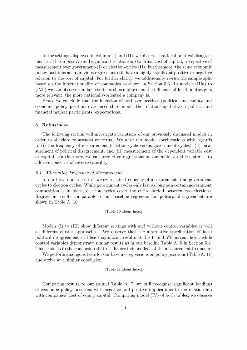
In the settings displayed in column (I) and (II), we observe that local political disagree-ment still has a positive and significant relationship to firms’ cost of capital, irrespective ofmeasurement over government-(I) or election-cycles (II). Furthermore, the same economicpolicy positions as in previous regressions still have a highly significant positive or negativerelation to the cost of capital. For further clarity, we additionally re-run the sample splitbased on the internationality of companies as shown in Section 5.3. In models (IIIa) to(IVb) we can observe similar results as shown above, as the influence of local politics getsmore relevant, the more nationally-oriented a company is.

Hence we conclude that the inclusion of both perspectives (political uncertainty andeconomic policy positions) are needed to model the relationship between politics andfinancial market participants’ expectations.

6. Robustness

The following section will investigate variations of our previously discussed models inorder to alleviate robustness concerns. We alter our model specifications with regardsto (i) the frequency of measurement (election cycle versus government cycles), (ii) mea-surement of political disagreement, and (iii) measurement of the dependent variable costof capital. Furthermore, we run predictive regressions on our main variables interest toaddress concerns of reverse causality.

6.1. Alternating Frequency of MeasurementIn our first robustness test we switch the frequency of measurement from government

cycles to election cycles. While government cycles only last as long as a certain governmentcomposition is in place, election cycles cover the entire period between two elections.Regression results comparable to our baseline regression on political disagreement areshown in Table A. 10.


Models (I) to (III) show different settings with and without control variables as wellas different cluster approaches. We observe that the alternative specification of localpolitical disagreement still leads significant results at the 1- and 5%-percent level, whilecontrol variables demonstrate similar results as in our baseline Table A. 5 in Section 5.2.This leads us to the conclusion that results are independent of the measurement frequency.

We perform analogous tests for our baseline regressions on policy positions (Table A. 11)and arrive at a similar conclusion.


Comparing results to our primal Table A. 7, we still recognize significant loadingsof economic policy positions with negative and positive implications to the relationshipwith companies’ cost of equity capital. Comparing model (IV) of both tables, we observe

20

that protectionist policies are still showing highly significant results, while the “Protec-tionism Negative” position even increases to the 1%-level of statistical significance, while“Economic Orthodoxy” takes on a coefficient significant at the 10%-level. The remain-ing observations do not portray any reason for the concern that results are driven bymeasurement over the election or government cycles, as they remain largely unchanged.

6.2. Alternative Measures for Political DisagreementA plausible caveat against the results presented in this study is related to our mea-

surement of local political uncertainty. It might be argued that results are driven by mea-surement peculiarities. We utilize two alternative measures, namely the average weightedstandard deviation of policy positions and Shannon’s H, which both have been introducedto the reader in Section 4. In order to attenuate these concerns, Table A. 12 presents ourbasic specifications using the alternative measures.


From left to right we show results of panel regressions first that use a weighted standarddeviation method, where the model shown in column (Ia) is specified without controls,while (Ib) provides results including controls. For both settings the alternative approxima-tion approach on local political disagreement yields equivalent results to our main section.Analogously, results remain unchanged if we approximate local uncertainty via Shannon’sH, as shown in (IIa) and (IIb), respectively.

6.3. Alternative Dependent VariablesAs discussed in Section 3.1.1, our main proxy for a company’s cost of capital is the

ICC . This measure is used because it is our intention to cover shifts in expectations ofmarket participants and investigate how these expectations are related to political char-acteristics within countries. We acknowledge that -although we view the ICC as the bestavailable proxy for cost of equity capital- there might be readers that demand results withmore conservative measures. We conduct our main analyses additionally using dividendyields, which we retrieve per company via Thomson Reuters/Datastream.29 We choosethe dividend yield as alternative measure because it contains information comparable toICC. Furthermore, given that dividends remain relatively stable over time, the measurecontains a significant forward-looking element. As for valid controls, we trim down thenumber of our previous controls discussed in Section 4.3 to a minimum set that shouldalso be relevant in the setting with dividend yield as the dependent variable. Results forour baseline setting are displayed in Table A. 13:


29Datastream field ”DY”.

21

Column (I) to (III) show our three different approaches to measure political disagree-ment in parliaments as introduced in Section 4. All three models contain year and firmfixed effects, the specified minimum set of controls as well as standard errors clustered atthe county level.30 While all controls show plausible coefficients, we can still observe asignificant positive relationship between local political disagreement -independent of themeasurement approach- and a company’s cost of equity capital. As results remain quali-tatively unchanged with respect to other specifications31, we conclude our findings remainrobust to the choice of dependent variables.

6.4. Focus on Years around ElectionsGiven that the political variables of interest change only relatively infrequently, we

should obtain similar results while only including the most relevant time periods in oursample. Consequently, we repeat our baseline regressions with a reduced sample includingonly observations from years around the election, namely the election year and the adjacentyears, i.e. one year prior and one year after the election year.


As can be seen from Table A. 14, the regression results remain virtually unchanged acrossall specifications

6.5. Reverse Causality TestsLastly, a major concern when interpreting previous regression results is reverse causal-

ity. As discussed in the literature review, previous researchers and their theoretical founda-tions suggest that instead of arguing that politics affecting financial markets, it is plausibleto establish a causal link in the opposite direction. Voters’ party preferences may be drivenby the current economic state. Anticipating such shifts, parties might adjust their politicalpositions accordingly. Or alternatively, difficult economic times could be associated withmore disagreement about economic policy within parliaments.


Following this logic, we should be able to predict political outcomes based on our mea-sure of firms’ cost of equity capital. To this end, we perform regressions with our keyvariables of interest as dependent variables. As explanatory variable we include the costof capital, and both GDP growth as well as inflation as control variables. All explanatoryvariables are lagged by one year. We only include observations of election years, as oth-erwise we would also include years where the dependent variable remains unchanged thatwould bias our results. Effectively, we try to predict national election outcomes based onthe cost of capital, GDP growth and inflation observed in the year prior to the election.

30Observations drop because dividend yields are only available for a subset of covered companies.31For the sake of brevity, we do not show all previous specifications with dividend yield again.

22

The regression results can be found in Table A. 15. Models (I) to (V) consider differentvariants of our political disagreement measure as dependent variable, while Models (VI) to(IX) focus on policy position variables. Across all regressions, with the exception of Model(VIII) with significance on the 10% level , we do not find any statistically significant rela-tionship between the political variables and the implied cost of capital. Consequently, eventhough we cannot fully exclude the issue of endogeneity, we do not find strong evidencethat the results presented throughout this paper are driven by reverse causality.

7. Conclusion

This paper examines the link between economic policy positions represented in na-tional parliaments and firms’ cost of equity capital based on a global, firm-level sample.Our study addresses various shortcomings of previous studies and provides new empiricalresults. Most importantly, we use a forward-looking measure to analyze the associationbetween economic policy and financial markets. We focus on investors’ risk perceptionrather than directional implications of policies for actual, but backward-looking outcomevariables. Measuring political disagreement within national parliaments as the dispersionof economic policy positions among parties, we show that higher levels of disagreementare associated with higher implied cost of equity capital. We perform a plausibility testby splitting our sample into subsamples based on the share of firms’ foreign sales to totalsales. We show that while the cost of capital of more domestically-oriented firms is af-fected, international firms are less affected by our measure of local political disagreement.The results imply that investors’ risk perception is higher during times of higher politicaldisagreement and that firms can reduce their exposure to political uncertainty by meansof geographical diversification.

Analogously, we analyze the representation of economic policy positions and theirassociation with investors’ risk perception. We find empirically significant associationsbetween six out of 16 policy positions and the implied cost of capital. Based on ourhypothesis that national sovereignty over the policies in question is a precondition for acausal link, we split our sample into EU countries and independent countries. We exploitthe fact that EU countries have delegated key economic policy competencies, such asinternational trade, to the EU parliament. We find that the relationship between economicpolicy positions and cost of capital fundamentally differs between the subsamples. Forexample, we show that an increase of protectionist tendencies within national parliamentsis associated with a significantly lower cost of capital for domestic firms, but only forcountries outside Europe. Within Europe, the empirically significant link points into theopposite direction. Our results are difficult to explain by political uncertainty alone butsuggest that economic policies can have a direct effect on investors’ perception of thefuture riskiness of firms. The empirical results presented in this paper are robust to avariety of alternative specifications of our dependent and independent variables. Tests ofreverse causality yield negative results. Our study provides the empirical groundwork forextending the current understanding of the link between politics and financial markets.We suggest future research to focus on two main areas: (i) disentangling indirect policy

23

uncertainty effects from direct effects of policies on the risk profile of economies, (ii)providing an empirical proof for a causal link between economic policy and the cost ofcapital.

24

8. Appendix (See Below)







25

References

Alesina, A., 1987. Macroeconomic Policy in a Two-Party System as a Repeated Game.The Quarterly Journal of Economics 102 (3), 651.

Alesina, A., 1997. Political Cycles and the Macroeconomy. MIT Press, Cambridge, Mass.

Alesina, A. F., Sachs, J. D., 1988. Political parties and the business cycle in the UnitedStates, 1948-1984. Journal of Money, Credit and Banking 20 (1), 63–82.

Azevedo, V. G., Bielstein, P., Gerhart, M., 2017. Earnings Forecasts: The Case for Com-bining Analysts’ Estimates with a Mechanical Model. Working Paper.

Baker, M., Bradley, B., Wurgler, J., 2011. Benchmarks as Limits to Arbitrage: Under-standing the Low-Volatility Anomaly. Financial Analysts Journal 67 (1), 40–54.

Baker, S. R., Bloom, N., Davis, S. J., 2016. Measuring Economic Policy Uncertainty.Working Paper (Stanford University).

Black, D., 1958. The Theory of Committees and Elections. Springer Netherlands, Dor-drecht.

Bosancianu, C. M., 2 2017. A Growing Rift in Values? Income and Educational Inequalityand Their Impact on Mass Attitude Polarization. Social Science Quarterly.

Boutchkova, M., Doshi, H., Durnev, A., Molchanov, A., 2012. Precarious politics andreturn volatility. Review of Financial Studies 25 (4), 1111–1154.

Brogaard, J., Detzel, A., 2015. The Asset-Pricing Implications of Government EconomicPolicy Uncertainty. Management Science 61 (1), 3–18.

Claus, J., Thomas, J., 2001. Equity Premia as Low as Three Percent? Evidence fromAnalysts’ Earnings Forecasts for Domestic and International Stock Markets. Journal ofFinance 56 (5), 1629–1666.

Core, J. E., Hail, L., Verdi, R. S., 2015. Mandatory disclosure quality, inside ownership,and cost of capital. European Accounting Review 24 (1), 1–29.

Croce, M. M., Kung, H., Nguyen, T. T., Schmid, L., 2012a. Fiscal policies and asset prices.Review of Financial Studies 25 (9), 2635–2672.

Croce, M. M., Nguyen, T. T., Schmid, L., 2012b. The market price of fiscal uncertainty.Journal of Monetary Economics 59 (5), 401–416.

Dinc, S. I., Erel, I., 2013. Economic Nationalism in Mergers and Acquisitions. Journal ofFinance 68 (6), 2471–2514.

Doring, H., Manow, P., 2016. Parliaments and governments database (ParlGov): Informa-tion on parties, elections and cabinets in modern democracies. Development version.

26

Easton, P. D., 2004. PE Ratios, PEG Ratios and Estimating the Implied Expected Rateof Return on Equity Capital. The Accounting Review 79 (1), 73–95.

Erb, C. B., Harvey, C. R., Viskanta, T. E., 11 1996. Political risk, economic risk, andfinancial risk. Financial Analysts Journal 52 (6), 29–46.

Fama, E. F., French, K. R., 1997. Industry costs of equity. Journal of Financial Economics43 (2), 153–193.

Finseraas, H., Vernby, K., 2011. What parties are and what parties do: Partisanship andwelfare state reform in an era of austerity. Socio-Economic Review 9 (4), 613–638.

Frank, M. Z., Shen, T., 2016. Investment and the weighted average cost of capital. Journalof Financial Economics 119 (2), 300–315.

Franzmann, S., Kaiser, A., 2006. Locating Political Parties in Policy Space: A Reanalysisof Party Manifesto Data. Party Politics 12 (2), 163–188.

Gebhardt, W. R., Lee, C. M. C., Swaminathan, B., 2001. Toward an Implied Cost ofCapital. Journal of Accounting Research 39 (1), 135–176.

Guay, W., Kothari, S. P., Shu, S., 2011. Properties of implied cost of capital using analysts’forecasts. Australian Journal of Management 36 (2), 125–149.

Hail, L., Leuz, C., 2006. International differences in the cost of equity capital: Do legalinstitutions and securities regulation matter? Journal of Accounting Research 44 (3),485–531.

Hayek, F., 1976. Denationalisation of Money: The Argument Refined. The Institute ofEconomic Affairs, London.

Herfindahl, O., 1950. Concentration in the U.S. steel industry. Ph.D. thesis, ColumbiaUniversity, New York.

Hibbs, D. A., 1977. Political Parties and Macroeconomic Policy. Source: The AmericanPolitical Science Review 71 (4), 1467–1487.

Hirschman, A. O., 1945. National Power and the Structur of Foreign Trade. University ofCalifornia Press, Berkley.

Hirschman, A. O., 1964. Paternity of an Index. The American Economic Review 54 (5),761–762.

Horn, A., Kevins, A., Jensen, C., Kersbergen, K. V., 12 2017. Peeping at the corpus –What is really going on behind the equality and welfare items of the Manifesto project?Journal of European Social Policy 27 (5), 403–416.

27

Jensen, C., Seeberg, H. B., 2015. The power of talk and the welfare state: Evidencefrom 23 countries on an asymmetric opposition-government response mechanism. Socio-Economic Review 13 (2), 215–233.

Julio, B., Yook, Y., 2012. Political Uncertainty and Corporate Investment Cycles. TheJournal of Finance 67 (1), 45–83.

Kenneth J. Arrow, 1952. Social Choice and Individual Values. Yale University Press, NewHaven and London.

Kropivnik, S., 2013. Comparison of Electoral Manifestos’ Issue Structures in Contempo-rary Democracies - the Methodological Perspective. Journal of Comparative Politics6 (1), 81–97.

Lee, C., Ng, D., Swaminathan, B., 2009. Testing International Asset Pricing Models UsingImplied Costs of Capital. Journal of Financial and Quantitative Analysis 44 (02), 307.

Leontief, W. W., 2 1941. The Structure of American Economy, 1919-1929: An EmpiricalApplication of Equilibrium Analysis. Harvard University Press, Cambridge, Mass.

Li, J., Born, J. A., 2006. Presidential election uncertainty and common stock returns inthe United States. Journal of Financial Research 29 (4), 609–622.

Li, X., 2015. Accounting Conservatism and the Cost of Capital: An International Analysis.Journal of Business Finance and Accounting 42 (5-6), 555–582.

Li, Y., Ng, D. T., Swaminathan, B., 2013. Predicting market returns using aggregateimplied cost of capital. Journal of Financial Economics 110 (2), 419–436.

Mikhaylov, S., Laver, M., Benoit, K. R., 2012. Coder reliability and misclassification inthe human coding of party manifestos. Political Analysis 20 (1), 78–91.

Myrdal, G., 1957. Economic Theory and Underdeveloped Regions. Duckworth, London.

Nordhaus, W. D., 12 1975. The Political Business Cycle. Review of Economic Studies42 (2), 169–191.

Ohlson, J. A., Juettner-Nauroth, B. E., 9 2005. Expected EPS and EPS Growth as De-terminantsof Value. Review of Accounting Studies 10 (2-3), 349–365.

Ortiz-Molina, H., Phillips, G. M., 2 2014. Real Asset Illiquidity and the Cost of Capital.Journal of Financial and Quantitative Analysis 49 (01), 1–32.

Pantzalis, C., Stangeland, D. A., Turtle, H. J., 2000. Political elections and the resolutionof uncertainty: The international evidence. Journal of Banking and Finance 24 (10),1575–1604.

28

Pastor, L., Sinha, M., Swaminathan, B., 12 2008. Estimating the Intertemporal Risk-Return Tradeoff Using the Implied Cost of Capital. The Journal of Finance 63 (6),2859–2897.

Pastor, L., Veronesi, P., 2012. Uncertainty about goverment policy and stock price. TheJournal of Finance 67 (4), 1219–1264.

Pastor, L., Veronesi, P., 2013. Political uncertainty and risk premia. Journal of FinancialEconomics 110 (3), 520–545.

Potrafke, N., 2016. Partisan politics: The empirical evidence from OECD panel studies.Journal of Comparative Economics.

Santa-Clara, P., Valkanov, R., 2003. The Presidential Puzzle: Political Cycles and theStock Market. The Journal of Finance 58 (5), 1841–1872.

Shannon, C. E., 1 1948. A mathematical theory of communication. The Bell System Tech-nical Journal 27 (July), 379–423.

Volkens, A., Lehmann, P., Matthieß, T., Merz, N., Regel, S., Weßels, B., 2017. TheManifesto Data Collection. Manifesto Project (MRG/CMP/MARPOR). Version 2017a.Wissenschaftszentrum Berlin fur Sozialforschung (WZB)., Berlin.

von dem Berge, B., Obert, P., 1 2017. Intraparty democracy in Central and EasternEurope. Party Politics, 1–11.

Werner, A., Lacewell, O., Volkens, A., 2015. Manifesto Coding Instructions (5th revisededition).

29

List of Figures

B. 1 Geographic coverage of our sample . . . . . . . . . . . . . . . . . . . . . . . 31B. 2 Development of Political Concentration Over Time and Selected Countries . 32B. 3 Description of Economic Policy Positions in the Manifesto Project Dataset . 33

30

Figure B. 1: Geographic coverage of our sample (blue)

31

Figure B. 2: Development of Political Concentration Over Time and Selected Countries

The depicted lines represent the Herfindahl-Hirschman Index of economic policy positions.A higher value of the HHI implies higher concentration of parties’ policy position andtherefore to a lower level of disagreement. In our regression analysis, we calculate theLocal Disagreement Index as HHI ∗ −1.

32

Figu

reB

.3:

Des

crip

tion

ofE

cono

mic

Polic

yPo

sitio

nsin

the

Man

ifest

oP

roje

ctD

atas

eta

a See

Volk

ens

etal

.(20

17).

33

List of Tables

A. 1 Overview of Domains and Party Policy Preferences in the Manifesto ProjectDataset . . . . . . . . . . . . . . . . . . . . . . . . . . . . . . . . . . . . . . 35

A. 2 Descriptive Statistics - Yearly Company Data . . . . . . . . . . . . . . . . . 36A. 3 Descriptive Statistics - Yearly Country Data . . . . . . . . . . . . . . . . . . 37A. 4 Overview of Countries and Elections Covered . . . . . . . . . . . . . . . . . 38A. 5 Political disagreement, measured as the dispersion of economic policy po-

sitions represented in the parliament, is related to higher implied cost ofequity capital. . . . . . . . . . . . . . . . . . . . . . . . . . . . . . . . . . . . 39

A. 6 International firms are less affected by (local) political disagreement. . . . . 40A. 7 The Relationship between the Representation of Economic Policy Positions

and Firms’ Cost of Equity Capital . . . . . . . . . . . . . . . . . . . . . . . 41A. 8 The Relationship between the Representation of Economic Policy Positions

and Firms’ Cost of Equity Capital. Sample Split EU-member states (Sov.= No) versus Independent Countries (Sov. = Yes). . . . . . . . . . . . . . . 42

A. 9 Combining Political Disagreement and Economic Policy Positions . . . . . . 43A. 10Political disagreement, measured as the dispersion of economic policy po-

sitions represented in the parliament, is related to higher implied cost ofequity capital. (Robustness Election Cycles) . . . . . . . . . . . . . . . . . . 44

A. 11The Relationship between the Representation of Economic Policy Positionsand Firms’ Cost of Equity Capital. (Robustness Election Cycles) . . . . . . 45

A. 12Political disagreement, measured via weighted standard deviation and Shan-non’s H, is related to higher implied cost of equity capital. (Robustnessindependent variables) . . . . . . . . . . . . . . . . . . . . . . . . . . . . . . 46

A. 13Political disagreement, measured as the dispersion of economic policy po-sitions represented in the parliament, is related to higher implied cost ofequity capital. (Robustness using dividend yield as dependent variable) . . 47

A. 14Combining Political Disagreement and Economic Policy Positions (Robust-ness: Focus on pre-election, election and post-election years) . . . . . . . . . 48

A. 15Reverse Causality Analysis (Robustness Predicting Political Variables withICC) . . . . . . . . . . . . . . . . . . . . . . . . . . . . . . . . . . . . . . . . 49

A. 16Definition of Variables . . . . . . . . . . . . . . . . . . . . . . . . . . . . . . 50A. 17Correlations of Economic Policy Positions . . . . . . . . . . . . . . . . . . . 52A. 18International firms are less affected by (local) political disagreement. (Ro-

bustness: Threshold foreign sales to total sales at 40%) . . . . . . . . . . . . 53A. 19International firms are less affected by (local) political disagreement. (Ro-

bustness: Threshold foreign sales to total sales at 50%) . . . . . . . . . . . . 54A. 20Overview of ICC computation methods (taken from Azevedo et al. (2017)) . 55

34

Table A. 1: Overview of Domains and Party Policy Preferences in the Manifesto Project Dataset

per401 Free Market Economy: Positiveper402 Incentives: Positiveper403 Market Regulation: Positiveper404 Economic Planning: Positiveper405 Corporatism: Positive

Domain 1: External Relations per406 Protectionism: PositiveDomain 2: Freedom and Democracy per407 Protectionism: NegativeDomain 3: Political System per408 Economic GoalsDomain 4: Economy per409 Keynesian Demand Mgmt.: PositiveDomain 5: Welfare and Quality of Life per410 Economic GrowthDomain 6: Fabric of Society per411 Technology and Infrastructure: PositiveDomain 7: Social Groups per412 Controlled Economy: Positive

per413 Nationalisation: Positiveper414 Economic Orthodoxy: Positiveper415 Marxist Analysis: Positiveper416 Anti-Growth Economy: Positive

Party policy preferences as available via the Manifesto dataset. Sub-categories are onlydisplayed for the domain “Economy”.

35

Table A. 2: Descriptive Statistics - Yearly Company Data

Obs. Mean σ P25 P50 P75

Dependent Variables

IccHail/Leuz 100,485 0.1117 0.0460 0.0830 0.1024 0.1293Dividend Yield 100,485 0.0213 0.0244 0.000 0.0148 0.0317

Company Controls

Return(12M) 100,485 0.1318 0.4865 -0.1661 0.0822 0.3518ln(Size) 100,485 13.8797 1.9459 12.4601 13.7637 15.1180ROA 100,485 0.0355 0.0776 0.0090 0.0346 0.0694Leverage 100,485 0.2220 0.1806 0.0603 0.2004 0.3429M/B 100,485 2.5155 2.4120 1.1559 1.7887 2.9023Turnover 100,485 250,426 567,376 10,101 49,832 198,479ElectionDomestic 100,485 0.2611 0.4392 0.0000 0.0000 1.0000Beta24 100,485 0.6190 0.6702 0.1602 0.5079 0.9682σ12M 100,485 0.3718 0.2049 0.2301 0.3216 0.4556BetaWorld24 100,485 0.9754 0.8350 0.4220 0.8876 1.4248

Descriptive Statistics are based on our baseline regression setting in Table A. 5, Model (II).

36

Table A. 3: Descriptive Statistics - Yearly Country Data

Obs. Mean σ P25 P50 P75

Political Uncertainty

Local Disagreement-IndexPers 454 -0.1880 0.0515 -0.2123 -0.1823 -0.1516Local Disagreement-IndexPers/Govcycle 454 -0.1885 0.0516 -0.2128 -0.1820 -0.1524Local Disagreement-IndexWSD 454 1.1060 0.4416 0.7600 0.9940 1.5063Local Disagreement-IndexWSD/Govcycle 454 1.0988 0.4378 0.7600 0.9573 1.5063Local Disagreement-IndexShan 454 0.7786 0.1692 0.6552 0.7903 0.8748Local Disagreement-IndexShan/Govcycle 454 0.7772 0.1696 0.6499 0.7916 0.8748

Economic Policy Positions

Free Market Economy 454 1.1048 1.1377 0.2370 0.6980 1.6308Incentives Positive 454 1.7471 1.6488 0.799 1.4679 2.0196Market Regulation 454 1.2788 1.2359 0.3923 0.9264 1.7192Economic Planning 454 0.2887 0.4929 0.0000 0.0695 0.4364Corporatism / Mixed Economy 454 0.1676 0.2333 0.0000 0.0554 0.3053Protectionism Positive 454 0.1161 0.3640 0.0000 0.0000 0.0394Protectionism Negative 454 0.1765 0.3260 0.0000 0.0576 0.2121Economic Goals 454 1.4019 1.7334 0.2384 0.9689 1.8873Keynesian Demand Management 454 0.1350 0.5165 0.0000 0.0000 0.0614Economic Growth Positive 454 1.2479 1.2744 0.3459 0.8081 1.9200Technology and Infrastructure: Positive 454 3.4136 2.0857 2.0307 3.0768 4.7049Controlled Economy 454 0.3148 0.9034 0.0000 0.0000 0.1649Nationalisation 454 0.1227 0.2621 0.0000 0.0000 0.1290Economic Orthodoxy 454 1.5126 1.6646 0.4044 0.9590 1.9434Marxist Analysis 454 0.0099 0.0739 0.0000 0.0000 0.0000Anti-Growth Economy Positive 454 0.2802 0.4890 0.0000 0.0121 0.3384

Country Level Control Variables

Inflation 454 2.1442 1.5645 1.2536 2.1040 2.8033∆GDP 454 2.1267 2.3522 0.9198 2.3660 3.5900

Descriptive Statistics are based on all available data points in our yearly dataset. Political positions shownare calculated for governments over government cycles.

37

Table A. 4: Overview of Countries and Elections Covered

Country name Political system Firstelectionincluded

Lastelectionincluded

Numberof elec-

tions

Numberof

observa-tions

Australia Parliamentary 1990 2013 9 6,983Austria Parliamentary 1990 2008 7 1,038Belgium Parliamentary 1991 2010 6 1,631Canada Parliamentary 1993 2011 7 8,347Denmark Parliamentary 1990 2011 7 1,859Finland Parliamentary 1987 2011 7 1,969France Parliamentary 1988 2012 6 8,053Germany Parliamentary 1990 2013 7 8,349Ireland Parliamentary 1992 2011 5 657Japan Parliamentary 1990 2014 9 28,145Netherlands Parliamentary 1994 2012 7 2,261New Zealand Parliamentary 1990 2011 8 1,147Norway Parliamentary 1989 2009 6 1,869Portugal Parliamentary 1991 2011 7 815Spain Parliamentary 1993 2011 6 2,226Sweden Parliamentary 1988 2010 7 3,301Switzerland Parliamentary 1991 2011 6 3,049United Kingdom Parliamentary 1987 2010 6 17,482United States Presidential 1988 2012 7 64,985

19 countries 18:01 Min:1987

Max:2014

130 164,166

38

Table A. 5: Political disagreement, measured as the dispersion of economic policy positions represented inthe parliament, is related to higher implied cost of equity capital.

VARIABLES (I) (II) (III)

Local Disagreement-IndexGovcycle 0.053*** 0.045*** 0.045**(3.33) (3.09) (2.70)

Return(12M) -0.019*** -0.019***(-12.5) (-8.67)

ln(Size) -0.0086** -0.0086**(-2.63) (-2.68)

ROA -0.017*** -0.017**(-3.41) (-2.73)

Leverage 0.034*** 0.034***(8.90) (8.05)

M/B -0.0032*** -0.0032***(-5.21) (-5.08)

Turnover 6.3e-09*** 6.3e-09***(6.36) (5.77)

Inflation 0.0012 0.0012(1.44) (1.31)

∆GDP -0.000072 -0.000072(-0.18) (-0.12)

Electiondomestic -0.00011 -0.00011(-0.14) (-0.11)

Beta24 -0.0013 -0.0013(-0.93) (-0.90)

σ12M 0.019*** 0.019***(5.39) (4.30)

BetaWorld24 0.0010 0.0010(1.47) (1.24)

Observations 159,623 100,485 100,485No. Cluster 19 19 19x25Adj.R2 0.42 0.49 0.49Adj.R2

within 0.0034 0.087 0.087

Fixed Effects Year Year YearFirm Firm Firm

Controls No Yes YesCluster Country Country Country-Year

The dependent variable is the ICC measure of Hail/Leuz (average of estimates). Year and firm fixed effects areincluded as indicated. Robust standard errors are clustered as displayed. The underlying estimation algorithmused by the command reghdfe removes the constant in the within transformation. Significance is indicated by ***,** and * at the 1%-, 5%- and 10%-level, respectively.

39

Table A. 6: International firms are less affected by (local) political disagreement.

(I) (I) (II) (II) (III) (III)VARIABLES < 30% >= 30% < 30% >= 30% < 30% >= 30%

LDIGovcycle 0.047*** 0.016 0.057*** 0.019 0.057*** 0.019*(5.49) (0.83) (4.95) (1.44) (3.85) (1.78)

Observations 25,862 38,323 20,265 31,353 20,265 31,353No. Clusters 19 19 19 19 19x25 19x25Adj.R2

within 0.0033 0.00031 0.092 0.077 0.092 0.078Adj.R2 0.47 0.42 0.53 0.47 0.53 0.47

Fixed Effects Year Year Year Year Year YearFirm Firm Firm Firm Firm Firm

Controls No No Yes Yes Yes YesCluster Country Country Country Country Country-

YearCountry-

Year

The dependent variable is the ICC measure of Hail/Leuz (average of estimates). All models are fixedeffect regressions. Year and firm dummies are included as indicated. Robust standard errors are clusteredas indicated. The underlying estimation algorithm used by the command reghdfe removes the constantin the within transformation. Significance is indicated by ***, ** and * at the 1%-, 5%- and 10%-level,respectively.

40

Table A. 7: The Relationship between the Representation of Economic Policy Positions and Firms’ Costof Equity Capital

VARIABLES (I) (II) (III) (IV)

Free Market Economy -0.0020* -0.0015 -0.0015(-1.74) (-1.48) (-1.23)

Incentives – Positive 0.00097 0.00048 0.00048(1.59) (0.73) (0.62)

Market Regulation 0.0018 0.0021** 0.0021** 0.0022**(1.69) (2.25) (2.13) (2.44)

Economic Planning 0.0045* 0.0036 0.0036(2.08) (1.71) (1.67)

Corporatism/Mixed Economy 0.0045 0.0011 0.0011(1.45) (0.39) (0.31)

Protectionism – Positive -0.012*** -0.010*** -0.010*** -0.0086***(-4.56) (-4.18) (-4.01) (-3.27)

Protectionism – Negative 0.0067** 0.0061*** 0.0061*** 0.0041*(2.72) (3.53) (3.01) (1.97)

Economic Goals -0.0010* -0.00070 -0.00070(-1.79) (-1.55) (-1.49)

Keynesian Demand Management 0.0035 0.0047 0.0047(1.35) (1.67) (1.60)

Economic Growth – Positive 0.0031*** 0.0017* 0.0017* 0.0014**(3.31) (1.93) (1.80) (2.87)

Technology and Infrastructure: Positive 0.0015*** 0.0015*** 0.0015** 0.0018***(3.17) (3.12) (2.36) (3.41)

Controlled Economy -0.00046 -0.0017 -0.0017(-0.14) (-0.56) (-0.56)

Nationalisation 0.0010 -0.0017 -0.0017(0.25) (-0.43) (-0.45)

Economic Orthodoxy 0.0011** 0.00072* 0.00072(2.17) (1.93) (1.47)

Marxist Analysis 0.0066 0.014*** 0.014*** 0.014***(1.40) (3.63) (3.05) (5.65)

Anti-Growth Economy – Positive 0.00057 0.00017 0.00017(0.28) (0.099) (0.072)

Observations 159,623 100,485 100,485 100,485No. Clusters 19 19 19x25 19Adj.R2

within 0.023 0.10 0.10 0.096Adj.R2 0.43 0.50 0.50 0.50

Fixed Effects Year Year Year YearFirm Firm Firm Firm

Controls No Yes Yes YesCluster Country Country Country-

YearCountry


41

Table A. 8: The Relationship between the Representation of Economic Policy Positions and Firms’ Costof Equity Capital. Sample Split EU-member states (Sov. = No) versus Independent Countries (Sov. =Yes).

(I) (I) (II) (II)VARIABLES Sov. = No Sov. = Yes Sov. = No Sov. = Yes

Free Market Economy -0.00023 -0.0029* -0.00023 -0.0029(-0.42) (-2.44) (-0.26) (-1.74)

Incentives – Positive 0.0011 -0.00068 0.0011 -0.00068(1.67) (-1.19) (1.49) (-1.02)

Market Regulation 0.00023 0.0047 0.00023 0.0047(0.35) (2.08) (0.35) (1.85)

Economic Planning 0.00091 0.0082 0.00091 0.0082(0.79) (1.71) (0.62) (1.72)

Corporatism/Mixed Economy -0.0024 -0.00069 -0.0024 -0.00069(-0.89) (-0.079) (-1.05) (-0.074)

Protectionism – Positive -0.00048 -0.012*** -0.00048 -0.012**(-0.096) (-5.83) (-0.11) (-4.40)

Protectionism – Negative -0.014 0.0065 -0.014* 0.0065(-1.74) (1.24) (-1.84) (1.12)

Economic Goals 0.0016** -0.0014 0.0016** -0.0014(2.47) (-1.93) (2.20) (-1.64)

Keynesian Demand Management -0.0036* 0.013*** -0.0036** 0.013*(-2.12) (4.62) (-2.63) (2.45)

Economic Growth – Positive -0.00018 0.0028*** -0.00018 0.0028**(-0.28) (6.35) (-0.25) (3.44)

Technology and Infrastructure: Positive 0.00027 0.0016** 0.00027 0.0016*(0.53) (3.19) (0.47) (2.39)

Controlled Economy 0.0031 -0.0097** 0.0031 -0.0097**(1.65) (-4.09) (1.64) (-2.85)

Nationalisation 0.0076*** -0.016 0.0076*** -0.016(3.46) (-1.23) (4.46) (-1.22)

Economic Orthodoxy 0.0010 0.00029 0.0010 0.00029(1.70) (0.57) (1.50) (0.34)

Marxist Analysis 0.021*** 0.021***(4.65) (4.56)

Anti-Growth Economy – Positive 0.0014 -0.0060 0.0014 -0.0060(0.96) (-0.82) (1.00) (-0.76)

Observations 32,809 67,676 32,809 67,676No. Clusters 14 5 14x24 5x25Adj.R2

within 0.092 0.12 0.092 0.12Adj.R2 0.46 0.52 0.46 0.52


Controls Yes Yes Yes YesCluster Country Country Country-Year Country-Year

The dependent variable is the ICC measure of Hail/Leuz (average of estimates). All models are fixed effectregressions. Year and firm dummies are included as indicated. Robust standard errors are clustered at the countrylevel. The underlying estimation algorithm used by the command reghdfe removes the constant in the withintransformation. Significance is indicated by ***, ** and * at the 1%-, 5%- and 10%-level, respectively. We classifythe United States, Australia, Canada, Japan, New Zealand and Israel as sovereign countries with respect to theirability to implement economic policies.

42

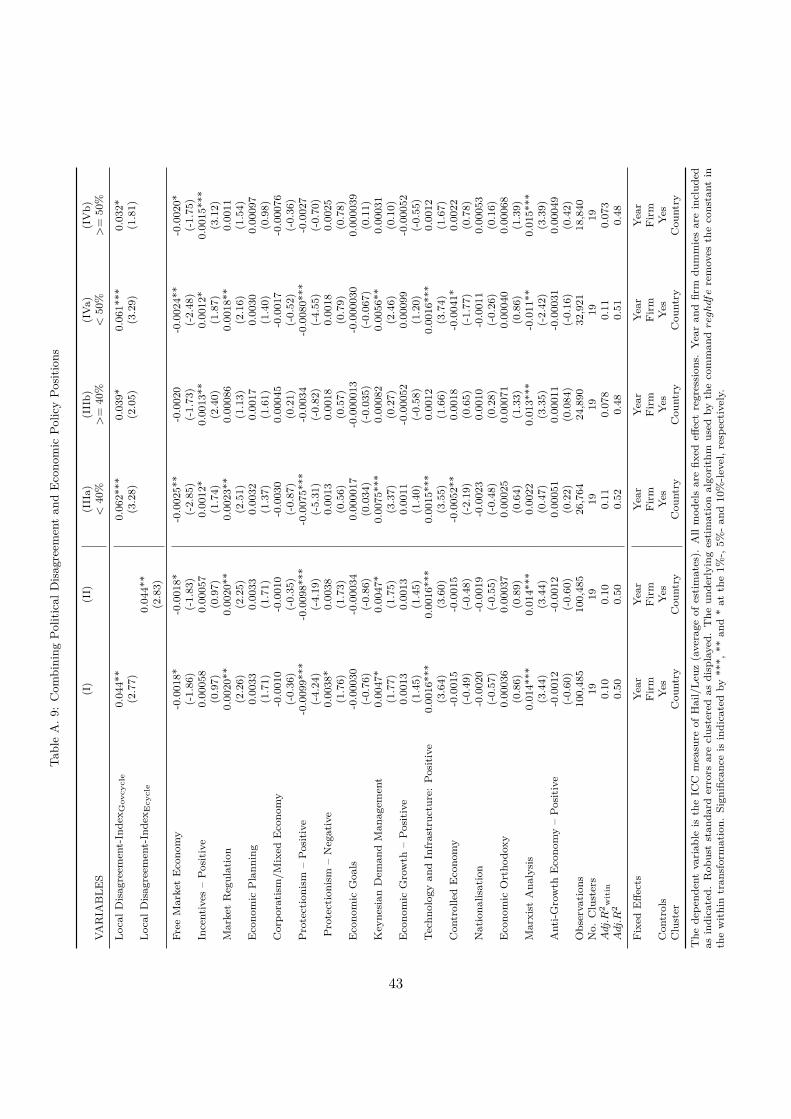
Tabl

eA

.9:

Com

bini

ngPo

litic

alD

isag

reem

ent

and

Eco

nom

icPo

licy

Posi

tions

(I)

(II)

(III

a)(I

IIb)

(IV

a)(I

Vb)

VAR

IAB

LES

<40

%>

=40

%<

50%

>=

50%

Loca

lDis

agre

emen

t-In

dex G

ovcy

cle

0.04

4**

0.06

2***

0.03

9*0.

061*

**0.

032*

(2.7

7)(3

.28)

(2.0

5)(3

.29)

(1.8

1)Lo

calD

isag

reem

ent-

Inde

x Ecy

cle

0.04

4**

(2.8

3)

Free

Mar

ket

Eco

nom

y-0

.001

8*-0

.001

8*-0

.002

5**

-0.0

020

-0.0

024*

*-0

.002

0*(-

1.86

)(-

1.83

)(-

2.85

)(-

1.73

)(-

2.48

)(-

1.75

)In

cent

ives

–P

osit

ive

0.00

058

0.00

057

0.00

12*

0.00

13**

0.00

12*

0.00

15**

*(0

.97)

(0.9

7)(1

.74)

(2.4

0)(1

.87)

(3.1

2)M

arke

tR

egul

atio

n0.

0020

**0.

0020

**0.

0023

**0.

0008

60.

0018

**0.

0011

(2.2

6)(2

.25)

(2.5

1)(1

.13)

(2.1

6)(1

.54)

Eco

nom

icP

lann

ing

0.00

330.

0033

0.00

320.

0017

0.00

300.

0009

7(1

.71)

(1.7

1)(1

.37)

(1.6

1)(1

.40)

(0.9

8)C

orpo

rati

sm/M

ixed

Eco

nom

y-0

.001

0-0

.001

0-0

.003

00.

0004

5-0

.001

7-0

.000

76(-

0.36

)(-

0.35

)(-

0.87

)(0

.21)

(-0.

52)

(-0.

36)

Pro

tect

ioni

sm–

Pos

itiv

e-0

.009

9***

-0.0

098*

**-0

.007

5***

-0.0

034

-0.0

080*

**-0

.002

7(-

4.24

)(-

4.19

)(-

5.31

)(-

0.82

)(-

4.55

)(-

0.70

)P

rote

ctio

nism

–N

egat

ive

0.00

38*

0.00

380.

0013

0.00

180.

0018

0.00

25(1

.76)

(1.7

3)(0

.56)

(0.5

7)(0

.79)

(0.7

8)E

cono

mic

Goa

ls-0

.000

30-0

.000

340.

0000

17-0

.000

013

-0.0

0003

00.

0000

39(-

0.76

)(-

0.86

)(0

.034

)(-

0.03

5)(-

0.06

7)(0

.11)

Key

nesi

anD

eman

dM

anag

emen

t0.

0047

*0.

0047

*0.

0075

***

0.00

082

0.00

56**

0.00

031

(1.7

7)(1

.75)

(3.3

7)(0

.27)

(2.4

6)(0

.10)

Eco

nom

icG

row

th–

Pos

itiv

e0.

0013

0.00

130.

0011

-0.0

0052

0.00

099

-0.0

0052

(1.4

5)(1

.45)

(1.4

0)(-

0.58

)(1

.20)

(-0.

55)

Tech

nolo

gyan

dIn

fras

truc

ture

:P

osit

ive

0.00

16**

*0.

0016

***

0.00

15**

*0.

0012

0.00

16**

*0.

0012

(3.6

4)(3

.60)

(3.5

5)(1

.66)

(3.7

4)(1

.67)

Con

trol

led

Eco

nom

y-0

.001

5-0

.001

5-0

.005

2**

0.00

18-0

.004

1*0.

0022

(-0.

49)

(-0.

48)

(-2.

19)

(0.6

5)(-

1.77

)(0

.78)

Nat

iona

lisat

ion

-0.0

020

-0.0

019

-0.0

023

0.00

10-0

.001

10.

0005

3(-

0.57

)(-

0.55

)(-

0.48

)(0

.28)

(-0.

26)

(0.1

6)E

cono

mic

Ort

hodo

xy0.

0003

60.

0003

70.

0002

50.

0007

10.

0004

00.

0006

8(0

.86)

(0.8

9)(0

.64)

(1.3

3)(0

.86)

(1.3

9)M

arxi

stA

naly

sis

0.01

4***

0.01

4***

0.00

220.

013*

**-0

.011

**0.

015*

**(3

.44)

(3.4

4)(0

.47)

(3.3

5)(-

2.42

)(3

.39)

Ant

i-Gro

wth

Eco

nom

y–

Pos

itiv

e-0

.001

2-0

.001

20.

0005

10.

0001

1-0

.000

310.

0004

9(-

0.60

)(-

0.60

)(0

.22)

(0.0

84)

(-0.

16)

(0.4

2)O

bser

vati

ons

100,

485

100,

485

26,7

6424

,890

32,9

2118

,840

No.

Clu

ster

s19

1919

1919

19Adj.R

2w

itin

0.10

0.10

0.11

0.07

80.

110.

073

Adj.R

20.

500.

500.

520.

480.

510.

48

Fix

edE

ffect

sY

ear

Yea

rY

ear

Yea

rY

ear

Yea

rF

irm

Fir

mF

irm

Fir

mF

irm

Fir

mC

ontr

ols

Yes

Yes

Yes

Yes

Yes

Yes

Clu

ster

Cou

ntry

Cou

ntry

Cou

ntry

Cou

ntry

Cou

ntry

Cou

ntry

The

depe

nden

tva

riab

leis

the

ICC

mea

sure

ofH

ail/

Leuz

(ave

rage

ofes

tim

ates

).A

llm

odel

sar

efix

edeff

ect

regr

essi

ons.

Yea

ran

dfir

mdu

mm

ies

are

incl

uded

asin

dica

ted.

Rob

ust

stan

dard

erro

rsar

ecl

uste

red

asdi

spla

yed.

The

unde

rlyi

nges

tim

atio

nal

gori

thm

used

byth

eco

mm

andreghdfe

rem

oves

the

cons

tant

inth

ew

ithi

ntr

ansf

orm

atio

n.Si

gnifi

canc

eis

indi

cate

dby

***,

**an

d*

atth

e1%

-,5%

-an

d10

%-le

vel,

resp

ecti

vely

.

43

Table A. 10: Political disagreement, measured as the dispersion of economic policy positions representedin the parliament, is related to higher implied cost of equity capital. (Robustness Election Cycles)


Local Disagreement-IndexEcycle 0.056*** 0.047*** 0.047**(3.15) (3.02) (2.65)

Return(12M) -0.019*** -0.019***(-12.6) (-8.68)

ln(Size) -0.0085** -0.0085**(-2.65) (-2.69)

ROA -0.017*** -0.017**(-3.41) (-2.74)

Leverage 0.034*** 0.034***(8.87) (8.03)

M/B -0.0032*** -0.0032***(-5.22) (-5.09)

Turnover 6.3e-09*** 6.3e-09***(6.40) (5.80)

Inflation 0.0011 0.0011(1.41) (1.28)

∆GDP -0.000047 -0.000047(-0.12) (-0.077)

Electiondomestic -0.00013 -0.00013(-0.16) (-0.13)

Beta24 -0.0013 -0.0013(-0.93) (-0.90)

σ12M 0.019*** 0.019***(5.40) (4.31)

BetaWorld24 0.0010 0.0010(1.47) (1.24)

Observations 159,623 100,485 100,485No. Cluster 19 19 19x25Adj.R2

within 0.0036 0.087 0.087Adj.R2 0.42 0.49 0.49


Controls No Yes YesCluster Country Country Country-Year


44

Table A. 11: The Relationship between the Representation of Economic Policy Positions and Firms’ Costof Equity Capital. (Robustness Election Cycles)


Free Market Economy -0.0019* -0.0014 -0.0014(-1.74) (-1.47) (-1.23)

Incentives – Positive 0.00096 0.00047 0.00047(1.62) (0.72) (0.61)

Market Regulation 0.0020 0.0022* 0.0022* 0.0022**(1.69) (2.10) (2.00) (2.40)

Economic Planning 0.0049** 0.0038* 0.0038* 0.0032**(2.49) (1.90) (1.80) (2.16)

Corporatism/Mixed Economy 0.0040 0.0012 0.0012(1.41) (0.41) (0.33)

Protectionism – Positive -0.013*** -0.011*** -0.011*** -0.0089***(-4.82) (-4.11) (-3.85) (-3.30)

Protectionism – Negative 0.0075*** 0.0064*** 0.0064*** 0.0058**(3.16) (3.93) (3.18) (2.86)

Economic Goals -0.00050 -0.00056 -0.00056(-0.62) (-0.74) (-0.66)

Keynesian Demand Management 0.0037 0.0049 0.0049(1.42) (1.72) (1.65)

Economic Growth – Positive 0.0033*** 0.0018* 0.0018* 0.0016***(3.39) (2.08) (1.95) (2.90)

Technology and Infrastructure: Positive 0.0016*** 0.0015*** 0.0015** 0.0018***(3.50) (3.38) (2.54) (3.57)

Controlled Economy -0.00014 -0.0018 -0.0018(-0.041) (-0.55) (-0.54)

Nationalisation 0.0010 -0.0014 -0.0014(0.28) (-0.37) (-0.38)

Economic Orthodoxy 0.0011** 0.00067 0.00067(2.15) (1.56) (1.28)

Marxist Analysis 0.0067 0.014*** 0.014** 0.015***(1.38) (3.20) (2.74) (4.61)

Anti-Growth Economy – Positive 0.00050 0.00018 0.00018(0.25) (0.11) (0.075)

Observations 159,623 100,485 100,485 100,485No. Clusters 19 19 19x25 19Adj.R2

within 0.023 0.10 0.10 0.097Adj.R2 0.43 0.50 0.50 0.50


Controls No Yes Yes YesCluster Country Country Country-

YearCountry


45

Table A. 12: Political disagreement, measured via weighted standard deviation and Shannon’s H, is relatedto higher implied cost of equity capital. (Robustness independent variables)


Local Disagreement-IndexWSD 0.014** 0.0086***(2.19) (3.10)

Local Disagreement-IndexShannon’s H 0.029** 0.020**(2.35) (2.43)

Observations 159,623 100,485 159,623 100,485No. Clusters 19 19 19 19Adj.R2 0.42 0.49 0.42 0.49Adj.R2

within 0.0052 0.087 0.0069 0.088


Controls No Yes No YesCluster Country Country Country Country

The dependent variable is the ICC measure of Hail/Leuz (average of estimates). Allmodels are fixed effect regressions. Year and firm dummies are included as indicated.Robust standard errors are clustered at the country level. The underlying estimationalgorithm used by the command reghdfe removes the constant in the within transforma-tion. Significance is indicated by ***, ** and * at the 1%-, 5%- and 10%-level, respectively.

46

Table A. 13: Political disagreement, measured as the dispersion of economic policy positions representedin the parliament, is related to higher implied cost of equity capital. (Robustness using dividend yield asdependent variable)


Local Disagreement-IndexGovcycle 0.020***(3.76)

Local Disagreement-IndexWSD 0.0041**(2.13)

Local Disagreement-IndexShan 0.0071***(4.09)

ln(Size) 0.0017* 0.0016* 0.0017*(1.79) (1.75) (1.79)

Inflation 0.0010*** 0.00066** 0.00071**(3.73) (2.26) (2.29)

∆GDP -0.00032 -0.00019 -0.00014(-1.04) (-0.72) (-0.48)

Return(12M) -0.0071*** -0.0070*** -0.0071***(-3.35) (-3.31) (-3.33)

Beta24 -0.0016*** -0.0016*** -0.0016***(-4.94) (-4.47) (-4.89)

σ12M -0.0010 -0.00092 -0.0010(-0.78) (-0.67) (-0.78)

BetaWorld24 0.000088 0.000015 0.000074(0.30) (0.057) (0.26)

Turnover -1.2e-09 -1.2e-09 -1.2e-09*(-1.69) (-1.58) (-1.74)

Observations 20,888 20,888 20,888Adj.R2

within 0.060 0.060 0.059Adj.R2 0.67 0.67 0.67


Controls Yes Yes YesCluster Country Country Country

The dependent variable is the dividend yield. Subsample used includes domestically-oriented firms witha share of foreign sales to total sales below 30%. Year and firm fixed effects are included as indicated.Robust standard errors are clustered as displayed. The underlying estimation algorithm used by thecommand reghdfe removes the constant in the within transformation. Significance is indicated by ***, **and * at the 1%-, 5%- and 10%-level, respectively.

47

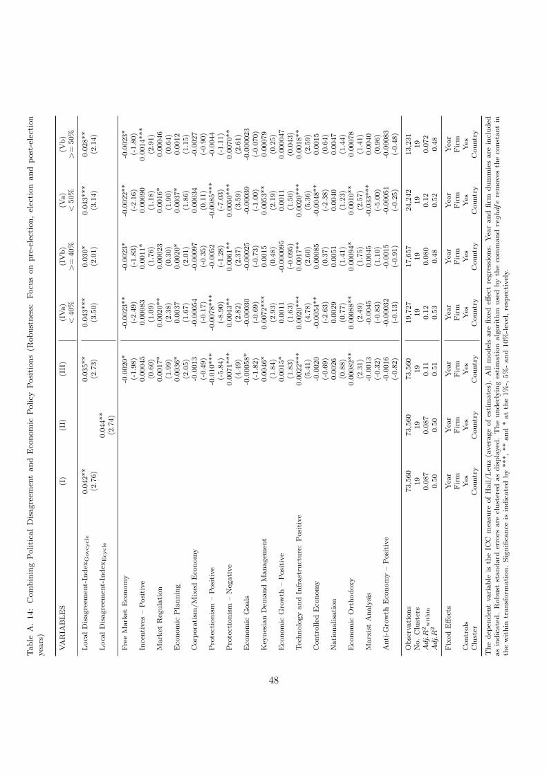
Tabl

eA

.14

:C

ombi

ning

Polit

ical

Dis

agre

emen

tan

dE

cono

mic

Polic

yPo

sitio

ns(R

obus

tnes

s:Fo

cus

onpr

e-el

ectio

n,el

ectio

nan

dpo

st-e

lect

ion

year

s)

VAR

IAB

LES

(I)

(II)

(III

)(I

Va)

(IV

b)(V

a)(V

b)<

40%

>=

40%

<50

%>

=50

%

Loca

lDis

agre

emen

t-In

dex G

ovcy

cle

0.04

2**

0.03

5**

0.04

3***

0.03

0*0.

043*

**0.

028*

*(2

.76)

(2.7

3)(3

.50)

(2.0

1)(3

.14)

(2.1

4)Lo

calD

isag

reem

ent-

Inde

x Ecy

cle

0.04

4**

(2.7

4)

Free

Mar

ket

Eco

nom

y-0

.002

0*-0

.002

3**

-0.0

023*

-0.0

022*

*-0

.002

3*(-

1.98

)(-

2.49

)(-

1.83

)(-

2.16

)(-

1.80

)In

cent

ives

–P

osit

ive

0.00

045

0.00

083

0.00

11*

0.00

090

0.00

14**

*(0

.60)

(1.0

9)(1

.76)

(1.1

8)(2

.91)

Mar

ket

Reg

ulat

ion

0.00

17*

0.00

20**

0.00

023

0.00

16*

0.00

046

(1.9

9)(2

.38)

(0.3

0)(1

.90)

(0.6

4)E

cono

mic

Pla

nnin

g0.

0036

*0.

0037

0.00

20*

0.00

37*

0.00

12(2

.05)

(1.6

7)(2

.01)

(1.8

6)(1

.15)

Cor

pora

tism

/Mix

edE

cono

my

-0.0

013

-0.0

0054

-0.0

0097

0.00

034

-0.0

027

(-0.

49)

(-0.

17)

(-0.

35)

(0.1

1)(-

0.90

)P

rote

ctio

nism

–P

osit

ive

-0.0

10**

*-0

.007

8***

-0.0

052

-0.0

085*

**-0

.004

4(-

5.84

)(-

8.90

)(-

1.28

)(-

7.03

)(-

1.11

)P

rote

ctio

nism

–N

egat

ive

0.00

71**

*0.

0043

**0.

0061

**0.

0050

***

0.00

70**

(4.4

9)(2

.82)

(2.3

7)(3

.59)

(2.6

1)E

cono

mic

Goa

ls-0

.000

58*

-0.0

0030

-0.0

0025

-0.0

0039

-0.0

0002

3(-

1.82

)(-

0.69

)(-

0.73

)(-

1.00

)(-

0.07

0)K

eyne

sian

Dem

and

Man

agem

ent

0.00

46*

0.00

72**

*0.

0015

0.00

53**

0.00

079

(1.8

4)(2

.93)

(0.4

8)(2

.19)

(0.2

5)E

cono

mic

Gro

wth

–P

osit

ive

0.00

15*

0.00

11-0

.000

095

0.00

110.

0000

47(1

.83)

(1.6

3)(-

0.09

5)(1

.50)

(0.0

43)

Tech

nolo

gyan

dIn

fras

truc

ture

:P

osit

ive

0.00

22**

*0.

0020

***

0.00

17**

0.00

20**

*0.

0018

**(5

.41)

(4.7

8)(2

.60)

(5.3

6)(2

.59)

Con

trol

led

Eco

nom

y-0

.002

0-0

.005

4**

0.00

085

-0.0

048*

*0.

0015

(-0.

69)

(-2.

63)

(0.3

7)(-

2.38

)(0

.64)

Nat

iona

lisat

ion

0.00

260.

0029

0.00

510.

0040

0.00

47(0

.88)

(0.7

7)(1

.41)

(1.2

3)(1

.44)

Eco

nom

icO

rtho

doxy

0.00

082*

*0.

0008

8**

0.00

094*

0.00

10**

0.00

078

(2.3

1)(2

.49)

(1.7

5)(2

.57)

(1.4

1)M

arxi

stA

naly

sis

-0.0

013

-0.0

045

0.00

45-0

.033

***

0.00

40(-

0.32

)(-

0.83

)(1

.10)

(-5.

00)

(0.9

6)A

nti-G

row

thE

cono

my

–P

osit

ive

-0.0

016

-0.0

0032

-0.0

015

-0.0

0051

-0.0

0083

(-0.

82)

(-0.

13)

(-0.

91)

(-0.

25)

(-0.

48)

Obs

erva

tion

s73

,560

73,5

6073

,560

19,7

2717

,657

24,2

4213

,231

No.

Clu

ster

s19

1919

1919

1919

Adj.R

2w

ithi

n0.

087

0.08

70.

110.

120.

080

0.12

0.07

2Adj.R

20.

500.

500.

510.

530.

480.

520.

48

Fix

edE

ffect

sY

ear

Yea

rY

ear

Yea

rY

ear

Yea

rY

ear

Fir

mF

irm

Fir

mF

irm

Fir

mF

irm

Fir

mC

ontr

ols

Yes

Yes

Yes

Yes

Yes

Yes

Yes

Clu

ster

Cou

ntry

Cou

ntry

Cou

ntry

Cou

ntry

Cou

ntry

Cou

ntry

Cou

ntry

The

depe

nden

tva

riab

leis

the

ICC

mea

sure

ofH

ail/

Leuz

(ave

rage

ofes

tim

ates

).A

llm

odel

sar

efix

edeff

ect

regr

essi

ons.

Yea

ran

dfir

mdu

mm

ies

are

incl

uded

asin

dica

ted.

Rob

ust

stan

dard

erro

rsar

ecl

uste

red

asdi

spla

yed.

The

unde

rlyi

nges

tim

atio

nal

gori

thm

used

byth

eco

mm

andreghdfe

rem

oves

the

cons

tant

inth

ew

ithi

ntr

ansf

orm

atio

n.Si

gnifi

canc

eis

indi

cate

dby

***,

**an

d*

atth

e1%

-,5%

-an

d10

%-le

vel,

resp

ecti

vely

.

48

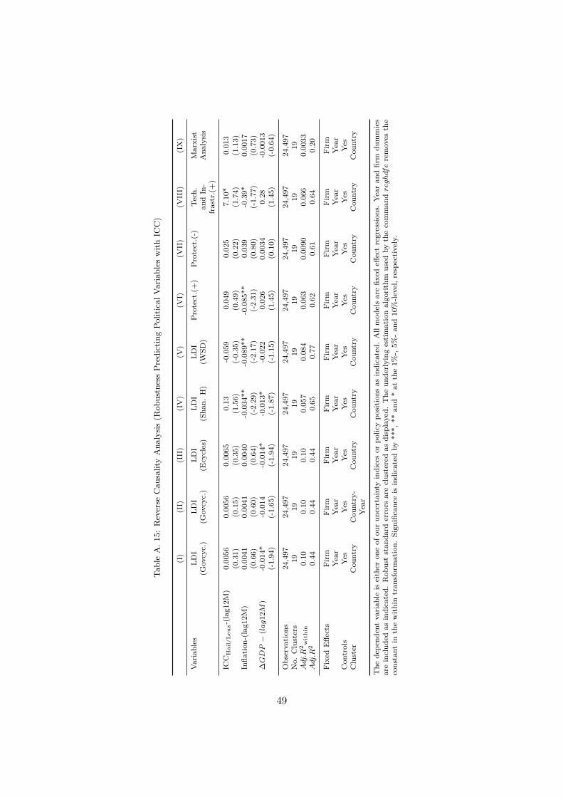
Tabl

eA

.15:

Rev

erse

Cau

salit

yA

naly

sis

(Rob

ustn

ess

Pre

dict

ing

Polit

ical

Varia

bles

with

ICC

)

(I)

(II)

(III

)(I

V)

(V)

(VI)

(VII

)(V

III)

(IX

)

Var

iabl

esLD

ILD

ILD

ILD

ILD

IP

rote

ct.(

+)

Pro

tect

.(-)

Tech

.M

arxi

st(G

ovcy

c.)

(Gov

cyc.

)(E

cycl

es)

(Sha

n.H

)(W

SD)

and

In-

fras

tr.(

+)

Ana

lysi

s

ICC

Hai

l/L

euz-

(lag

12M

)0.

0056

0.00

560.

0065

0.13

-0.0

590.

049

0.02

57.

10*

0.01

3(0

.31)

(0.1

5)(0

.35)

(1.5

6)(-

0.35

)(0

.49)

(0.2

2)(1

.74)

(1.1

3)In

flati

on-(

lag1

2M)

0.00

410.

0041

0.00

40-0

.034

**-0

.089

**-0

.085

**0.

039

-0.3

9*0.

0017

(0.6

6)(0

.60)

(0.6

4)(-

2.29

)(-

2.17

)(-

2.31

)(0

.80)

(-1.

77)

(0.7

3)∆GDP

−(lag12M

)-0

.014

*-0

.014

-0.0

14*

-0.0

13*

-0.0

220.

026

0.00

340.

28-0

.001

3(-

1.94

)(-

1.65

)(-

1.94

)(-

1.87

)(-

1.15

)(1

.45)

(0.1

0)(1

.45)

(-0.

64)

Obs

erva

tion

s24

,497

24,4

9724

,497

24,4

9724

,497

24,4

9724

,497

24,4

9724

,497

No.

Clu

ster

s19

1919

1919

1919

1919

Adj.R

2w

ithi

n0.

100.

100.

100.

057

0.08

40.

063

0.00

900.

066

0.00

33Adj.R

20.

440.

440.

440.

650.

770.

620.

610.

640.

20

Fix

edE

ffect

sF

irm

Fir

mF

irm

Fir

mF

irm

Fir

mF

irm

Fir

mF

irm

Yea

rY

ear

Yea

rY

ear

Yea

rY

ear

Yea

rY

ear

Yea

rC

ontr

ols

Yes

Yes

Yes

Yes

Yes

Yes

Yes

Yes

Yes

Clu

ster

Cou

ntry

Cou

ntry

-Y

ear

Cou

ntry

Cou

ntry

Cou

ntry

Cou

ntry

Cou

ntry

Cou

ntry

Cou

ntry

The

depe

nden

tva

riab

leis

eith

eron

eof

our

unce

rtai

nty

indi

ces

orpo

licy

posi

tion

sas

indi

cate

d.A

llm

odel

sar

efix

edeff

ect

regr

essi

ons.

Yea

ran

dfir

mdu

mm

ies

are

incl

uded

asin

dica

ted.

Rob

ust

stan

dard

erro

rsar

ecl

uste

red

asdi

spla

yed.

The

unde

rlyi

nges

tim

atio

nal

gori

thm

used

byth

eco

mm

andreghdfe

rem

oves

the

cons

tant

inth

ew

ithi

ntr

ansf

orm

atio

n.Si

gnifi

canc

eis

indi

cate

dby

***,

**an

d*

atth

e1%

-,5%

-an

d10

%-le

vel,

resp

ecti

vely

.

49

Table A. 16: Definition of Variables

Variable Description

Firm level data

IccHail/Leuz Mean of ICC measures; cf. Section 4.2Dividend Yield End-of-year dividend yield (DY )Return(12M) Cumulative total return over past 12 months.ln(Size) Natural logarithm of total assets (wc02999)ROA (Net Income bottom line / Total Assets) =

(wc01651/wc02999)Leverage (Total Debt / Total Assets) =

(wc03255/WC02999)M/B (Market Value of Equity / Common Equity) =

(wc08001 / wc03501)Turnover Trading Turnover over the last 12 months by vol-

umeElectionDomestic Dummy variable for election years per respective

countryBeta24 Beta of company’s monthly returns and country

index returns over the last 24 monthsσ12M Fill in description hereBetaWorld24 Beta of company’s monthly returns and MSCI

Global index returns over the last 24 months

Country-level data

Inflation Year-on-year change in annual consumer prices∆GDP Year-on-year change in GDP per country

Political Disagreement

Local Disagreement-IndexEcycle Local political disagreement index calculated overall parties in parliament via election cycles; cf.Section 5.2

Local Disagreement-IndexGovcycle Local political disagreement index calculated overall parties in parliament via government cycles; cf.Section 5.2

Local Disagreement-IndexWSD/Ecycle Local political disagreement index calculated asweighted standard deviation over all parties inparliament via election cycles; cf. Section 5.2

Local Disagreement-IndexWSD/Govcycle Local political disagreement index calculated asweighted standard deviation over all parties inparliament via government cycles; cf. Section 5.2

50

Definition of Variables - continuedVariable DescriptionLocal Disagreement-IndexShan/Ecycle Local political disagreement index calculated as

Shannon’s H over all parties in parliament viaelection cycles; cf. Section 5.2

Local Disagreement-IndexShan/Govcycle Local political disagreement index calculated asShannon’s H over all parties in parliament viagovernment cycles; cf. Section 5.2

51

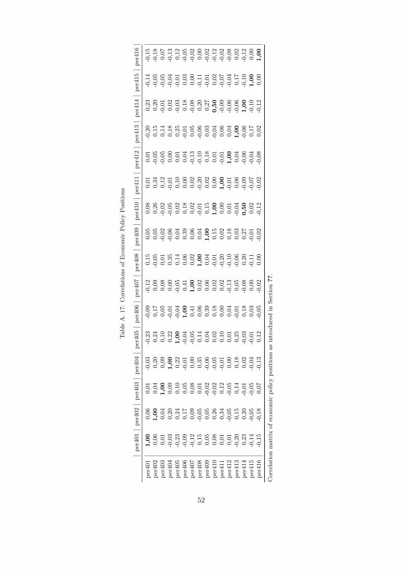
Tabl

eA

.17:

Cor

rela

tions

ofE

cono

mic

Polic

yPo

sitio

ns

per4

01pe

r402

per4

03pe

r404

per4

05pe

r406

per4

07pe

r408

per4

09pe

r410

per4

11pe

r412

per4

13pe

r414

per4

15pe

r416

per4

011,

000,

060,

01-0

,03

-0,2

3-0

,09

-0,1

20,

150,

050,

080,

010,

01-0

,20

0,23

-0,1

4-0

,15

per4

020,

061,

000,

040,

200,

240,

170,

09-0

,05

0,05

0,26

0,34

-0,0

50,

150,

20-0

,05

-0,1

8pe

r403

0,01

0,04

1,00

0,09

0,10

0,05

0,08

0,01

-0,0

2-0

,02

0,12

-0,0

50,

14-0

,01

-0,0

50,

07pe

r404

-0,0

30,

200,

091,

000,

22-0

,01

0,00

0,35

-0,0

6-0

,05

-0,0

10,

000,

180,

02-0

,04

-0,1

3pe

r405

-0,2

30,

240,

100,

221,

00-0

,04

-0,0

50,

140,

040,

020,

100,

010,

25-0

,03

-0,0

10,

12pe

r406

-0,0

90,

170,

05-0

,01

-0,0

41,

000,

410,

060,

390,

180,

000,

04-0

,01

0,18

0,03

-0,0

5pe

r407

-0,1

20,

090,

080,

00-0

,05

0,41

1,00

0,02

0,06

0,02

0,02

-0,1

30,

05-0

,08

0,00

-0,0

2pe

r408

0,15

-0,0

50,

010,

350,

140,

060,

021,

000,

04-0

,01

-0,2

0-0

,10

-0,0

60,

20-0

,11

0,00

per4

090,

050,

05-0

,02

-0,0

60,

040,

390,

060,

041,

000,

150,

020,

180,

030,

27-0

,01

-0,0

2pe

r410

0,08

0,26

-0,0

2-0

,05

0,02

0,18

0,02

-0,0

10,

151,

000,

000,

01-0

,04

0,50

0,02

-0,1

2pe

r411

0,01

0,34

0,12

-0,0

10,

100,

000,

02-0

,20

0,02

0,00

1,00

-0,0

10,

06-0

,09

-0,0

7-0

,02

per4

120,

01-0

,05

-0,0

50,

000,

010,

04-0

,13

-0,1

00,

180,

01-0

,01

1,00

0,04

-0,0

6-0

,04

-0,0

8pe

r413

-0,2

00,

150,

140,

180,

25-0

,01

0,05

-0,0

60,

03-0

,04

0,06

0,04

1,00

-0,0

60,

170,

02pe

r414

0,23

0,20

-0,0

10,

02-0

,03

0,18

-0,0

80,

200,

270,

50-0

,09

-0,0

6-0

,06

1,00

-0,1

0-0

,12

per4

15-0

,14

-0,0

5-0

,05

-0,0

4-0

,01

0,03

0,00

-0,1

1-0

,01

0,02

-0,0

7-0

,04

0,17

-0,1

01,

000,

00pe

r416

-0,1

5-0

,18

0,07

-0,1

30,

12-0

,05

-0,0

20,

00-0

,02

-0,1

2-0

,02

-0,0

80,

02-0

,12

0,00

1,00

Cor

rela

tion

mat

rixof

econ

omic

polic

ypo

sitio

nsas

intr

oduc

edin

Sect

ion

??.

52

Table A. 18: International firms are less affected by (local) political disagreement. (Robustness: Thresholdforeign sales to total sales at 40%)

(I) (I) (II) (II) (III) (III)VARIABLES < 40% >= 40% < 40% >= 40% < 40% >= 40%

LDIGovcycle 0.048*** 0.011 0.055*** 0.013 0.055*** 0.013(5.61) (0.55) (5.16) (0.91) (4.08) (1.17)

Return(12M) -0.019*** -0.018*** -0.019*** -0.018***(-10.1) (-8.30) (-7.20) (-6.53)

ln(Size) -0.0091** -0.0076*** -0.0091** -0.0076***(-2.57) (-4.01) (-2.60) (-4.01)

ROA -0.023*** -0.015*** -0.023*** -0.015**(-6.39) (-3.66) (-3.57) (-2.51)

Leverage 0.030*** 0.041*** 0.030*** 0.041***(5.72) (6.70) (4.96) (6.10)

M/B -0.0031*** -0.0029*** -0.0031*** -0.0029***(-4.55) (-5.87) (-4.52) (-5.31)

Turnover 5.9e-09*** 6.3e-09** 5.9e-09*** 6.3e-09(8.50) (2.19) (4.80) (1.64)

Inflation 0.0015 0.0014** 0.0015 0.0014*(1.68) (2.31) (1.57) (1.94)

∆GDP -0.00030 0.00032 -0.00030 0.00032(-0.66) (0.61) (-0.43) (0.51)

Electiondomestic -0.00085 -0.00057 -0.00085 -0.00057(-0.79) (-0.73) (-0.72) (-0.51)

Beta24 -0.0022* -0.0021 -0.0022* -0.0021(-1.83) (-1.32) (-1.77) (-1.20)

σ12M 0.018*** 0.017*** 0.018*** 0.017***(3.70) (4.55) (2.95) (4.57)

BetaWorld24 0.0011 0.00055 0.0011 0.00055(1.61) (0.62) (1.25) (0.58)


within 0.0035 0.00012 0.092 0.071 0.092 0.071Adj.R2 0.46 0.42 0.52 0.47 0.52 0.47



YearCountry-

Year

The dependent variable is the ICC measure of Hail/Leuz (average of estimates). All models are fixed effectregressions. Year and firm dummies are included as indicated. Robust standard errors are clustered asdisplayed. The underlying estimation algorithm used by the command reghdfe removes the constant in thewithin transformation.Significance is indicated by ***, ** and * at the 1%-, 5%- and 10%-level, respectively.

53

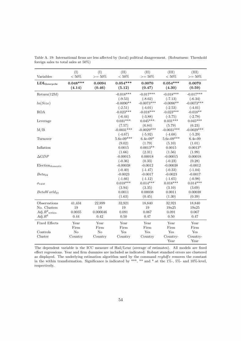
Table A. 19: International firms are less affected by (local) political disagreement. (Robustness: Thresholdforeign sales to total sales at 50%)

(I) (I) (II) (II) (III) (III)Variables < 50% >= 50% < 50% >= 50% < 50% >= 50%

LDIGovcycle 0.048*** 0.0094 0.054*** 0.0070 0.054*** 0.0070(4.14) (0.46) (5.12) (0.47) (4.30) (0.59)

Return(12M) -0.018*** -0.017*** -0.018*** -0.017***(-9.53) (-8.62) (-7.13) (-6.34)

ln(Size) -0.0090** -0.0073*** -0.0090** -0.0073***(-2.51) (-4.01) (-2.53) (-4.01)

ROA -0.023*** -0.018*** -0.023*** -0.018**(-6.44) (-3.88) (-3.75) (-2.78)

Leverage 0.031*** 0.045*** 0.031*** 0.045***(7.57) (6.84) (5.79) (6.23)

M/B -0.0031*** -0.0029*** -0.0031*** -0.0029***(-4.67) (-5.92) (-4.68) (-5.29)

Turnover 5.6e-09*** 6.4e-09* 5.6e-09*** 6.4e-09(9.02) (1.79) (5.10) (1.01)

Inflation 0.0015 0.0013** 0.0015 0.0013*(1.66) (2.31) (1.56) (1.99)

∆GDP -0.00015 0.00018 -0.00015 0.00018(-0.36) (0.33) (-0.23) (0.28)

Electiondomestic -0.00038 -0.0012 -0.00038 -0.0012(-0.40) (-1.47) (-0.33) (-1.04)

Beta24 -0.0023 -0.0017 -0.0023 -0.0017(-1.66) (-1.12) (-1.65) (-0.98)

σ12M 0.018*** 0.014*** 0.018*** 0.014***(3.94) (3.35) (3.10) (3.69)

BetaWorld24 0.0011 0.00038 0.0011 0.00038(1.63) (0.45) (1.30) (0.39)


within 0.0035 0.000046 0.091 0.067 0.091 0.067Adj.R2 0.44 0.42 0.50 0.47 0.50 0.47



YearCountry-

Year

The dependent variable is the ICC measure of Hail/Leuz (average of estimates). All models are fixedeffect regressions. Year and firm dummies are included as indicated. Robust standard errors are clusteredas displayed. The underlying estimation algorithm used by the command reghdfe removes the constantin the within transformation. Significance is indicated by ***, ** and * at the 1%-, 5%- and 10%-level,respectively.

54

Table A. 20: Overview of ICC computation methods (taken from Azevedo et al. (2017))

Model Formulas and Implementation Details Source

GLS

Mt = Bt +11∑τ=1

Et[ROEt+τ − ICC ×Bt+τ−1](1 + ICC)k + Et[(ROEt+12 − ICC) ×Bt+11]

ICC × (1 + ICC)11 (6)

where Mt is the market equity in year t. ICC is the Implied Cost of Cap-ital. Bt is the book equity. Et[] represents market expectations based oninformation available in year t, and (ROEt+τ − ICC) × Bt+τ−1, denotesthe residual income in year (t + τ), i.e., the difference between the returnon book equity and the ICC multiplied by the book equity in the previousyear. We compute the ROE from years t+1 to t+3 as FEPSt/Bt−1, wherethe FEPSt is the consensus mean I/B/E/S analysts‘ earnings per share ofperiod t. After year t+3, we linearly fade for the next nine years to a tar-get industry median. We calculate this proxy as a rolling industry medianover 5 years, considering only firms that have a positive ROE. Our indus-try definition is based on Fama and French (1997). Finally, after the periodt+12, the terminal value is a simply perpertuity of the residual incomes. Weestimate the book value based on clean surplus accounting and a constantpayout ratio PO, i.e., Bt = Bt−1 + FEPSt + (1 − PO).

Gebhardtet al.(2001)

CT

Mt = Bt +5∑τ=1

Et[ROEt+τ − ICC ×Bt+τ−1](1 + ICC)k + Et[(ROEt+5 − ICC) ×Bt+4](1 + g)

(ICC − g) × (1 + ICC)5 (7)

where Mt is the market equity in year t. ICC is the Implied Cost ofCapital. Bt is the book equity. Et[] represents market expectations basedon information available in year t, and (ROEt+τ − ICC) ×Bt+τ−1), denotesthe residual income in year t + τ , i.e., the difference between the return onbook equity and tee ICC multiplied by the book equity in the previous year.We compute the ROE from years t+1 to t+5 as FEPSt/Bt−1, where theFEPSt is the consensus mean I/B/E/S analysts‘ earnings per share of periodt. we estimate the forecasts in the years t+4 and t+5 using a long-termgrowth forecast, g, and the three-year ahead forecast. We estimate g as 10-year government bond minus an assumed real risk-free rate of three percent.Finally, after the period t+5, the terminal value is a simply perpetuity ofthe residual incomes. We estimate the book value based on clean surplusaccounting and a constant payout ratio PO, i.e., Bt = Bt−1 +FEPSt+(1−PO).

ClausandThomas(2001)

55

Overview of ICC computation methods - continuedModel Formulas and Implementation Details SourceMPEG

Mt = Et[Et+2] + ICC × Et[Dt+1] − Et[Et+1]ICC2 (8)

where Mt is the market equity in year t. ICC is the Implied Cost of Capital.Et[] represents market expectations based on information available in year t,Et+1 and Et+2 are, the earnings forecast in years t+1 and t+2, respectively.Dt+1 is the dividend in year t+1.

Easton(2004)

OJ

ICC = A+√A2 + Et[Et+1]

Mt+ (g − (γ − 1)) (9)

where: A = 0.5((γ − 1) + Et[Dt+1]Mt

), Mt is the market equity in year t. ICCis the Implied Cost of Capital. Et[] represents market expectations based oninformation available in year t, Et+1 is the earnings forecast in years t+1.Dt+1 is the dividend in year t+1. g is the short-term growth, computedas the rate between EPSt+1 and EPSt+2. γ is the perpetual growth ratein abnormal earnings beyond the forecast horizon, calculated as 10-yeargovernment bond minus an assumed real risk-free rate of three percent.

OhlsonandJuettner-Nauroth(2005)

56

political uncertainty and beyond: the relationship of economic annual meetings/2018-milan... ·...

Documents