ECONOMIC GROWTH CENTER

YALE UNIVERSITY

P.O. Box 208629 New Haven, CT 06520-8269

http://www.econ.yale.edu/~egcenter/

CENTER DISCUSSION PAPER NO. 997

Political Mergers as Coalition Formation

Eric Weese Yale University

April 2011

Notes: Center discussion papers are preliminary materials circulated to stimulate

discussion and critical comments. This paper originated as a thesis chapter. I would like to thank my thesis committee: Daron Acemoglu, Abhijit Banerjee, and Esther Duflo. I would also like to thank attendees at seminar presentations for their helpful comments, and the members of the MIT Political Economy working group for support, encouragement, and further useful suggestions. This research was supported by a Canadian Institute for Advanced Research junior fellowship and a Japan Society for the Promotion of Science postdoctoral fellowship. The latter was held at Hitotsubashi University on the invitation of Masayoshi Hayashi, who, along with Masashi Nishikawa, explained to me the details of the Japanese local public finance system. Thanks to Vadim Marmer and Francesco Trebbi for pointing out an econometric error in an earlier version of this paper, and Alberto Alesina and Nancy Qian for suggestions regarding the structure and text. Konrad Menzel offered valuable comments regarding econometric strategies. Computational support was provided by the Yale Faculty of Arts and Science High Performance Computing facilities, based on initial computations performed at MIT.

Political Mergers as Coalition Formation*

Eric Weese†

March 2011

Abstract

Political coalition formation games can describe the formation and dissolu-tion of nations, as well as the creation of coalition governments, the establish-ment of political parties, and other similar phenomena. These games have beenstudied from a theoretical perspective, but the resulting models have not beenused extensively in empirical work. This paper presents a method of estimat-ing political coalition formation models with many-player coalitions, and thenillustrates this method by estimating structural coefficients that describe thebehaviour of municipalities during a recent set of municipal mergers in Japan.The method enables counterfactual analysis, which in the Japanese case showsthat the national government could increase welfare via a counter-intuitive pol-icy involving transfers to richer municipalities conditional on their participationin a merger.

JEL codes: C63, D71, H77Keywords: Computational Techniques, Coalitions, Municipalities

*This paper originated as a thesis chapter. I would like to thank my thesis committee: DaronAcemoglu, Abhijit Banerjee, and Esther Duflo. I would also like to thank attendees at seminarpresentations for their helpful comments, and the members of the MIT Political Economy workinggroup for support, encouragement, and further useful suggestions. This research was supported by aCanadian Institute for Advanced Research junior fellowship and a Japan Society for the Promotionof Science postdoctoral fellowship. The latter was held at Hitotsubashi University on the invitationof Masayoshi Hayashi, who, along with Masashi Nishikawa, explained to me the details of theJapanese local public finance system. Thanks to Vadim Marmer and Francesco Trebbi for pointingout an econometric error in an earlier version of this paper, and Alberto Alesina and Nancy Qian forsuggestions regarding the structure and text. Konrad Menzel offered valuable comments regardingeconometric strategies. Computational support was provided by the Yale Faculty of Arts and ScienceHigh Performance Computing facilities, based on initial computations performed at MIT.

†Economics Department, Yale University. Email: eric.weese@yale.edu.

1

1 IntroductionIssues related to political coalition formation have recently attracted considerableinterest from theorists and policy makers. For example, the formation and dissolu-tion of countries can be seen as a political coalition formation game, with coalitionsconsisting of residents of a geographic area [Alesina and Spolaore, 1997]. The ques-tion of how many countries ought to exist and where borders should be drawn hascurrent relevance in places such as Georgia or Sudan, and recent episodes such asthe dissolution of Yugoslavia can be explained using a coalition formation framework[Desmet, Breton, Ortuno-Ortin, and Weber, 2009]. The formation of a governmentalso corresponds to a political coalition formation game, with the political partiesbeing the players. Similarly, parties could themselves be viewed as resulting from anunderlying political coalition formation game, this time with individual legislators asthe players [Merlo, 2006].

Changes to the rules governing the coalition formation game may lead to a differentand more efficient coalition structure. Any analysis of the effect of such changesrequires knowledge of the underlying structural parameters and an understandingof the process of coalition formation given various possible sets of rules.1 In orderto evaluate different potential rules it is first necessary to develop a model of thebehaviour of the players participating in the coalition formation game. This modelcan then be used to predict the changes in behaviour that would result from theimposition of different sets of rules.

Although models of coalition formation date back at least to von Neumann andMorgenstern [1944], relatively few empirical papers have made use of such models,and these papers have tended not to examine the effect of possible changes in therules of the coalition formation game being studied.2 Desirable properties of somespecific forms of coalition formation games, such as two-sided matching games, haveled to extensive empirical study of those game forms [Roth, 2008], but empiricalresearch on more general coalition formation models has been hampered by the fact

1For example, a recurring proposal in Canada is that members of parliament should be requiredto stand for a by-election if changing their party affiliation between general elections. Had this rulebeen in place during recent parliaments, different coalition structures might have resulted, leadingto different governments and policy outcomes. Similarly, different laws regarding how municipalitiescan cooperate to provide public goods, or how farmers can establish agricultural cooperatives, couldlead to different coalition structures with different welfare implications.

2Diermeier, Eraslan, and Merlo [2003] is an interesting exception.

2

that neither existence nor uniqueness of a stable coalition structure is guaranteed,and the number of coalition structures increases exponentially with the number ofplayers. Recently, Fox [2008] and related papers have studied coalition formationgames with transferrable utility, which is particularly relevant for issues in industrialorganization. This paper studies games where transfers are not possible, the casewhich is more relevant for issues in political economy [Acemoglu, 2003].

This paper presents a method of estimating the structural parameters of a politicalcoalition formation model and then applies it to a recent set of Japanese municipalmergers. In the Heisei Daigappei, individual Japanese municipalities could choosewhat merger if any they wished to participate in, given a fixed set of national gov-ernment transfer policies. The parameters that determine municipal preferences overmergers are estimated, and these estimates are then used to predict the effect of al-ternative national government transfer policies. The Heisei mergers are particularlyattractive from a modelling perspective, as government policy led to mergers occur-ring only during 1999-2010, and thus the resulting coalition structure can plausiblybe treated as the outcome of a single period coalition formation game.3 Furthermore,the mergers are of interest from a policy perspective, since due to efficiencies of scalethe smaller municipalities spend over ¥1,000,000 per capita per year providing thesame services that larger municipalities provide for slightly over ¥100,000, and al-most all of this difference was being subsidized by the national government.4 Thus, inaddition to a new method of analyzing political coalition formation games, the paperalso contributes the specific analysis of an economically interesting case.

The methodological contribution consists of the use of simulated maximum likeli-3In general, a problem with applying political coalition formation models to observed data is that

political coalitions once formed tend to persist, and changes that do occur are often separated bylarge time periods. The extremely high cost of any realignment means that the stability of exist-ing borders does not provide much information, and it is not clear what it means for there to bea “stable” coalition structure, if changes to this structure occur over time at a slow but constantrate. The Japanese data used in this paper mostly avoids this problem. The fiscal crisis of the1990s precipitated such significant changes in intergovernmental transfers that in many cases theold municipal borders were effectively untenable, thus leading to a very large number of mergersduring the window when mergers were allowed. Furthermore, during the 1970-1995 period, nationalpolicy had made municipal mergers extremely unattractive, and thus boundaries remained effec-tively unchanged even though demographic changes were rendering these boundaries increasinglyinefficient.

4For comparisons, ¥1=1¢ is a rough but useful approximation. During the period in whichfinancial data is analyzed, the USD/JPY exchange rate has varied from ¥147=$1 (Aug. ’98) to¥80=$1 (Oct. ’10). GDP per capita has remained relatively constant at ¥4,000,000.

3

hood estimation to obtain structural parameters describing players’ preferences overcoalitions when the observed coalition structure can be treated as the outcome ofa Bogomolnaia and Jackson [2002] hedonic coalition formation game. Two ways ofovercoming problems related to non-existence or multiplicity of stable coalition struc-tures are considered. The first method is to assume that all players have the samepreferences over coalitions, resulting in the existence of a unique stable coalition struc-ture [Farrell and Scotchmer, 1988]. This is the approach used by Gordon and Knight[2009], but replacing their method of moments estimator with a simulated maximumlikelihood estimator makes it computationally feasible to examine mergers involvingmore than two players.5 However, the restriction that all players must have the samepreferences over coalitions does not work well in the Japanese case, where many lo-cal government services are provided at a single specific physical location (city hall,library, health centre, etc.). Surveys suggest that residents of municipalities at thegeographic “edge” of a proposed merger were concerned about the distance to post-merger public facilities, while residents of more centrally located municipalities werenot. This implies an Alesina and Spolaore [1997] style model, where players’ idealpoints are distributed over a geographic policy space. The arrangement of jurisdic-tions is then the result of a tradeoff between economies of scale in the provision ofpublic goods, and heterogeneity in preferences over the location of those goods.

A second strategy is thus developed, which allows players’ preferences over coali-tions to differ, but restricts the types of blocking coalitions that can form. This guar-antees existence but not uniqueness of a stable coalition structure [Ray and Vohra,1997], and thus estimation requires an assumption regarding which one of the setof stable coalition structures is actually selected. The advantage of this approach,however, is that the utility function can include interactions between individual andcoalition characteristics, and thus geographic distance to a Banks and Duggan [2005]generalized median voter can be included.6 This provides a direct link between a

5This is because the method of moments approach requires computing the stable coalition struc-ture repeatedly as part of the estimation process. The computational advantage of the simulatedmaximum likelihood approach, however, does not necessarily hold for all datasets: in some casesa very large number of simulations might be required to reduce simulation bias to an acceptablelevel, thereby making the method of moments approach more attractive. In the case of the Japanesedata used in this paper, SML estimates even with very few simulations (eg. R = 10) appear to giveacceptable results.

6The distributional assumption regarding idiosyncratic preferences also differs, with shocks beingi.i.d by municipality by coalition, rather than i.i.d by coalition as in the first approach. The correla-tion between idiosyncratic preferences regarding a given coalition is thus 0 rather than 1; however,

4

theoretically consistent model of jurisdiction formation and the estimating equationas actually implemented.

These two strategies are then applied to Japanese municipal merger data, with thecost of providing public services derived from existing national government estimates.Geographical features of the data allow the set of possible coalitions to be reducedto the point where the model is computationally tractable. The resulting parameterestimates differ depending on the estimation strategy used. Some of the coefficientsestimated by restricting preferences (following Farrell and Scotchmer [1988]) haveopposite sign to what would be expected, while those estimated by relaxing the re-quirements for stability (following Ray and Vohra [1997]) have the expected sign andplausible magnitudes. Monte Carlo exercises show that a majority of this differencecan be explained by the inability to include relevant variables within the restrictedpreferences framework.7

In general, in non-transferable utility coalition formation games there are oftencoalitions that, if formed, would increase the utility of some players by large amounts,but these coalitions do not form because some other participants in the coalitionwould end up with slightly lower utility. Thus, national government interventioncould lead to different and better coalition structures forming. The structural pa-rameters estimated are used to examine the effects of two counterfactual policies.First, the possibility of national government enforcement of transfers is considered,where the national government allows decentralized negotiations over these transfersto take place between municipalities. In this case, where the game is converted into atransferable-utility game, the outcome depends on the bargaining power of differenttypes of municipalities. While this policy increases the number mergers that occur, italso leads to potentially very large transfers from poor municipalities to richer ones,and the exact amount of the transfers cannot be known in advance without know-ing the bargaining method by which municipalities divide the benefits of a merger.Even under the most optimistic assumptions regarding bargaining power, the poorestmunicipalities end up worse off than under the original policy.

it is not clear that this is an improvement.7An earlier version of this paper [Weese, 2008] focused on variables that Kido and Nakamura

[2008] and other previous studies had identified as important: population, surface area, etc.. Plausi-ble coefficient estimates for those variables were obtained using the restricted preferences approach,but it is very difficult to respond to the Lucas critique while still satisfying the restricted preferencesconditions.

5

Next, an alternative is considered where the national government provides anadditional financial incentive for municipalities to participate in mergers. A samplebudget-balanced policy results in higher utility (equivalent on average to an increasein income of 0.4%) for both poor and rich municipalities, even though incentives toparticipate in mergers are only offered to relatively richer municipalities. This result issomewhat counter-intuitive as the problem the national government was attemptingto solve was the high cost of supporting small, poor municipalities. A regressiveconditional transfer – taxing everyone and transferring money to the residents ofricher municipalities that participate in mergers – is not an obvious response to thisproblem. The result is consistent with theory, however, since an incentive for richermunicipalities to merge with their neighbours will lead to those neighbours benefittingfrom higher levels of public goods. Providing an incentive to richer municipalitiesmimics the transfers that the municipalities themselves offered in the transferableutility game, but with amounts that are not as large. Thus, fewer mergers occur,but the poorer municipalities are on average better off than in the transferable utilitycase because they do not have to pay huge transfers to richer municipalities.8

The major contribution of this paper is to develop an empirical framework for theestimation of political coalition formation models that takes into account theoreticalcharacteristics of solutions and allows for the analysis of counterfactual policies. Inaddition to Gordon and Knight [2009], closely related papers are Brasington [1999]and Saarimaa and Tukiainen [2010], which use the maximum likelihood estimatorfrom Poirier [1980] and are thus restricted to considering each pairwise merger inisolation from other potential mergers.9 Other recent empirical political coalitionformation papers generally focus on describing patterns that are observed in polit-ical boundaries, while this paper estimates structural parameters and predicts howcounterfactual policies would change the set of boundaries forming.10 With suit-

8This result is related to the theory presented by Armstrong and Vickers [2010] regarding anti-trust regulation of corporate mergers; however, in the Armstrong and Vickers model, the cost ofallowing certain mergers to happen is that other, better, mergers do not occur, whereas in the modelpresented below, the primary cost of having more mergers occur is the ever larger transfers to richermunicipalities that must be provided. The transferable utility case thus has “too many” mergers, atleast for some social welfare functions.

9In models of the type used by Brasington and others, the probability that players 1 and 2 willform a coalition is unaffected by the other options that 1 or 2 might have. The method presentedbelow and that used by Gordon and Knight appear to be the only ones that take into account thatthe presence of a player 3 and an attractive {1, 3} coalition may disrupt a {1, 2} coalition that wouldotherwise form.

10Most empirical studies of political mergers thus far focus on American school districts. Miceli

6

able modifications, the method used in this paper could be applied to other types ofcoalition formation games, possibly in other fields as well as in political economy.

The rest of the paper has the following structure. The general estimation strategyis presented in Section 2, including both the version imposing a restriction on theform of players’ preferences and the version using instead a restriction on the types ofblocking coalitions. The use of this strategy in the Japanese case is then described inSection 3, including an analysis of potential alternative national government policiesusing counterfactual simulations. Section 4 concludes.

2 TheoryNotation follows that of Banerjee, Konishi, and Sönmez [2001]. Specifically, let N

be the set of players, and S ⊂ N a coalition of these players. Π is the set of allpossible coalition structures, where a coalition structure π ∈ Π is a set of coalitions{S1, . . . , SK} such that every player is in exactly one of these coalitions. Supposethat player i ∈ N has preferences ⪯i defined over the set {S ⊂ N |i ∈ S}, with ≺i

indicating a strict preference. The extension of these preferences to partitions is easy:if π(i) is the coalition that municipality i belongs to in partition π, then π ⪯i π′

if π(i) ⪯i π′(i). Let π ≺S π′ for some coalition S if ∀i ∈ S, π ⪯i π′ and at leastone of these preferences is strict. The observed coalition structure is treated as theresult of a pure hedonic coalition formation game, where the payoff to each playerdepends only on the coalition to which it belongs, and not on what other coalitionsoccur. This is the game introduced by Dreze and Greenberg [1980], except withoutthe possibility of even within-coalition transfers. The inability to negotiate transfersprevents some coalitions from forming:

Example 1. Let N = {1, 2}, and ui be a utility function describing the preferencesof player i over coalitions, with

u1({1, 2}) = u1({1}) + ϵ1,

u2({1, 2}) = u2({2}) + ϵ2. (1)

[1993], the earliest example yet found, examines the trade-off that Connecticut school districts facedbetween efficiencies of scale and locally optimal education quality. Alesina, Baqir, and Hoxby [2004]use a much larger dataset, and examine the relationship between county-level heterogeneity and thenumber of school districts and other local jurisdictions. While the estimates in each of these papersimply a type of coalition formation game, they do not present an explicit coalition formation model.

7

If ϵ1 > 0, ϵ2 < 0, |ϵ1| > |ϵ2|, then the stable coalition structure is {{1, 2}} if transfersare possible, but {{1}, {2}} if they are prohibited.

Ideally, given a set of preferences, there would exist a unique stable partition:First, the solution set is defined using the von Neumann and Morgenstern [1944]“stable set”:

Definition 1. ΠVNM is a stable set with respect to (Π, <) for some binary operator< if

1. ∄π, π′ ∈ ΠVNM where π < π′. (Internal stability)

2. ∀π /∈ ΠVNM, ∃π′ ∈ ΠVNM where π < π′. (External stability)

The goal is to define < in a way that is intuitively plausible yet at the same timeguarantees that the stable set exists, but this turns out not to be trivial. Consider,for example, the following definition of <: π < π′ if ∃S ∈ π′ such that π ≺S π′

and ∀S ′ ∈ (π \ π′), (S ′ \ S) ∈ π′ or is empty. Unfortunately, with this definition notonly is a stable set not guaranteed to exist, but in general it is not possible to deviseanother plausible method of selecting a single partition as the solution of this typeof coalition formation game [Barberà and Gerber, 2007]. The following “roommatesproblem” illustrates this point:

Example 2 (Gale and Shapley 1962). Suppose N = {1, 2, 3} and preferences are

{1, 2, 3} ≺1 {1} ≺1 {1, 3} ≺1 {1, 2},

{1, 2, 3} ≺2 {2} ≺2 {1, 2} ≺2 {2, 3},

{1, 2, 3} ≺3 {3} ≺3 {2, 3} ≺3 {1, 3}. (2)

With these preferences, no stable partition exists.

Nevertheless, when the Japanese municipalities actually played a coalition for-mation game, an outcome did occur. The problem is then how to treat observedoutcomes such as this one when attempting to estimate parameters. There are atleast four ways to proceed: to move to a non-cooperative game structure, to acceptset identification rather than point identification, to restrict preferences, or to relaxthe requirements for stability.

8

A non-cooperative game is guaranteed to provide a set of equilibrium outcomes,but it is difficult to use in this case as little information is available about the way inwhich the municipalities actually negotiated, or who made what offers, and so forth.Thus, the specification of the rules of the game would be essentially arbitrary. Ifthe equilibria did not depend on the rules, then the lack of information about thenegotiation process would not be important, but it is fairly easy to see that in this sortof coalition formation game, different rules produce different outcomes. For example,if there are a finite number of periods in which a proposer can propose a coalition orcoalition structure, then the probability with which various municipalities are selectedto be the proposer will change the types of proposals made and accepted. Radicallydifferent parameter estimates could be obtained by using different probabilities ofhaving a municipality selected as proposer, and there is no information availableon what reasonable proposer weights would be, or even whether the proposer typeframework is appropriate.11

Another intriguing possibility is that of set identification via moment inequalities,following the framework described by Pakes [2010]. This appears attractive, as thefact that {1, 2} is observed implies that {1} ≺1 {1, 2} and {2} ≺2 {1, 2} under a largevariety of equilibrium assumptions. However, in addition to this sort of inequalityshowing that municipalities do not want to be “too small”, in order to identify abounded set it is also necessary to find inequalities that show that municipalities donot wish to be “too big”. This is more challenging than it first appears, as it is truethat {{1}, {2}} observed implies that either {1, 2} ≺1 {1} or {1, 2} ≺2 {2}, but itis not clear which of these hold. Designing an error structure that both rational-izes the observed mergers while at the same time allowing estimation using this sortof “either-or” style inequalities is non-trivial, as the most obvious option requires adistributional assumption regarding the error term, thereby eliminating a major ad-vantage of the moment inequalities approach.12 This, combined with the Ponomarevaand Tamer critique regarding model misspecification, are the major reasons why this

11These critiques could also be applied to the choice of stability requirements used in the coop-erative form game analyzed in this paper. Estimators based on a cooperative form game, however,appear to be computationally simpler to implement than estimators based on a non-cooperative formgame. Thus, in the absence of reasons to choose a non-cooperative form game, the paper defaultsto the easier cooperative form game.

12There is also the possibility of using a model that cannot rationalize all the observed mergers, butit is not clear whether this has significant advantages over a fully-specified model with a sufficientlyfat-tailed error term.

9

paper focuses on a maximum likelihood approach, using either restricted preferences(“RP” from here on) or relaxed stability requirements (“RSR”).

2.1 Restricted Preferences

For the RP approach, consider the following restrictions on the form of ui, the utilitythat player i derives from a coalition:

ui(S) = u(S) + αi,

u(S) = v(XS; θ) + ϵS, (3)

where v is a function of characteristics XS of S, taking parameters θ.The econometrician observes XS and knows the functional form of v, and the

objective is to estimate the parameters θ. The error term ϵS is iid of a known distri-bution. The important restriction here is that if S ≺i S

′ then ∀j, S ≺j S′. That is,

all agents have identical preferences over coalitions.

Theorem 1 (Farrell and Scotchmer 1988). If all agents have identical preferencesover coalitions, a generically unique stable partition exists.

Proof. Exactly as given in Farrell and Scotchmer [1988], but repeated in AppendixA because it is a proof by construction, and the algorithm will be used to constructcounterfactual partitions later on.

The restriction on the idiosyncratic error term is strong: it implies that the ob-served and unobserved characteristics of a coalition are enjoyed equally by all itsmembers. In particular, in the case of municipal mergers it rules out the possibilitythat a large municipality merging with a smaller neighbour might take advantage of itselectoral power within the new amalgamated municipality in order to geographicallyskew locations of new public facilities. The major benefit of placing this restriction onthe error term is that it guarantees uniqueness, and thus estimation does not requireany assumption about an equilibrium selection rule.13

13It might be possible to weaken the restrictions on the error term somewhat by instead assumingthe monotonic median voter property [Acemoglu, Egorov, and Sonin, 2008], but the details of thisare not immediately obvious.

10

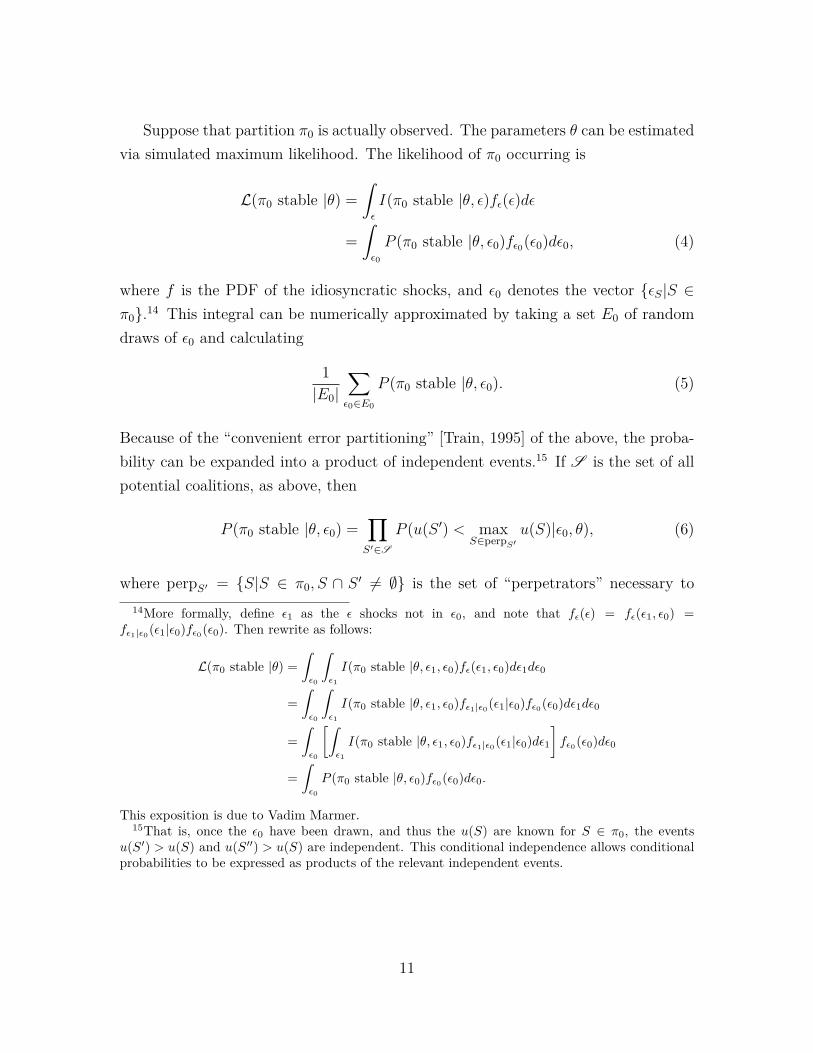
Suppose that partition π0 is actually observed. The parameters θ can be estimatedvia simulated maximum likelihood. The likelihood of π0 occurring is

L(π0 stable |θ) =∫ϵ

I(π0 stable |θ, ϵ)fϵ(ϵ)dϵ

=

∫ϵ0

P (π0 stable |θ, ϵ0)fϵ0(ϵ0)dϵ0, (4)

where f is the PDF of the idiosyncratic shocks, and ϵ0 denotes the vector {ϵS|S ∈π0}.14 This integral can be numerically approximated by taking a set E0 of randomdraws of ϵ0 and calculating

1

|E0|∑ϵ0∈E0

P (π0 stable |θ, ϵ0). (5)

Because of the “convenient error partitioning” [Train, 1995] of the above, the proba-bility can be expanded into a product of independent events.15 If S is the set of allpotential coalitions, as above, then

P (π0 stable |θ, ϵ0) =∏S′∈S

P (u(S ′) < maxS∈perpS′

u(S)|ϵ0, θ), (6)

where perpS′ = {S|S ∈ π0, S ∩ S ′ = ∅} is the set of “perpetrators” necessary to14More formally, define ϵ1 as the ϵ shocks not in ϵ0, and note that fϵ(ϵ) = fϵ(ϵ1, ϵ0) =

fϵ1|ϵ0(ϵ1|ϵ0)fϵ0(ϵ0). Then rewrite as follows:

L(π0 stable |θ) =∫ϵ0

∫ϵ1

I(π0 stable |θ, ϵ1, ϵ0)fϵ(ϵ1, ϵ0)dϵ1dϵ0

=

∫ϵ0

∫ϵ1

I(π0 stable |θ, ϵ1, ϵ0)fϵ1|ϵ0(ϵ1|ϵ0)fϵ0(ϵ0)dϵ1dϵ0

=

∫ϵ0

[∫ϵ1

I(π0 stable |θ, ϵ1, ϵ0)fϵ1|ϵ0(ϵ1|ϵ0)dϵ1]fϵ0(ϵ0)dϵ0

=

∫ϵ0

P (π0 stable |θ, ϵ0)fϵ0(ϵ0)dϵ0.

This exposition is due to Vadim Marmer.15That is, once the ϵ0 have been drawn, and thus the u(S) are known for S ∈ π0, the events

u(S′) > u(S) and u(S′′) > u(S) are independent. This conditional independence allows conditionalprobabilities to be expressed as products of the relevant independent events.

11

deviate to S ′. The likelihood function used for optimization is thus

L(π0 stable |θ) = 1

|E0|∑ϵ0∈E0

∏S′∈S

P (u(S ′) < maxS∈perpS′

u(S)|ϵ0, θ). (7)

2.2 Relaxed stability requirements

For the RSR approach, suppose that a less restrictive form is imposed on preferences:

ui(S) = v(Xi, XS; θ) + ϵiS (8)

where ϵiS are iid draws from a known distribution. Here, the utility a player derivesfrom a coalition can depend on interactions between the player’s characteristics andthose of the coalition, and similarly the ϵ for a given coalition can vary across players.In this case, the existence, but not uniqueness of a stable partition can be guaranteedso long as some restrictions are placed on the types of blocking coalitions that canform. In particular, only two types of potential deviations will be considered whenevaluating whether a given partition is stable: refinements, where a subcoalition of asingle existing coalition breaks off to form a coalition, and coarsenings, where two ormore existing coalitions merge in order to form a new coalition.

To guarantee existence, Ray and Vohra [1997] only allow deviating coalitions toforce refinements of a partition, and Diamantoudi and Xue [2007] show that thiscreates a stable set.16 Because hedonic games are simpler than the “equilibriumcoalition structures” that Ray and Vohra examine, refinements and coarsenings willbe treated identically. Otherwise, the theory follows that presented in Ray and Vohra.Let π ↗S π′ and π ↘S π′ mean that π ≺S π′, S ∈ π′, where π′ is a coarsening and arefinement of π, respectively. Using the terminology of Ray and Vohra, π is blockedby π′ if either there is a set of coalitions in π that are unanimously in favour of mergingto create π′, or there is a subset of “perpetrators” in π that are unanimously in favourof deviating from their current coalition. In the former case, π′ is the coarsening thatresults from the merger, while in the latter it is a refinement that includes a coalitionfor these perpetrators and some arrangement of the “residual” left behind when the

16An alternative approach would be to allow only single player deviations, as in Greenberg [1979].Ray and Vohra [1997] is used instead because anecdotal evidence suggests that multi-player devia-tions involving a refinement or a coarsening were more common than single player deviations not toa refinement or a coarsening during the coalition formation process.

12

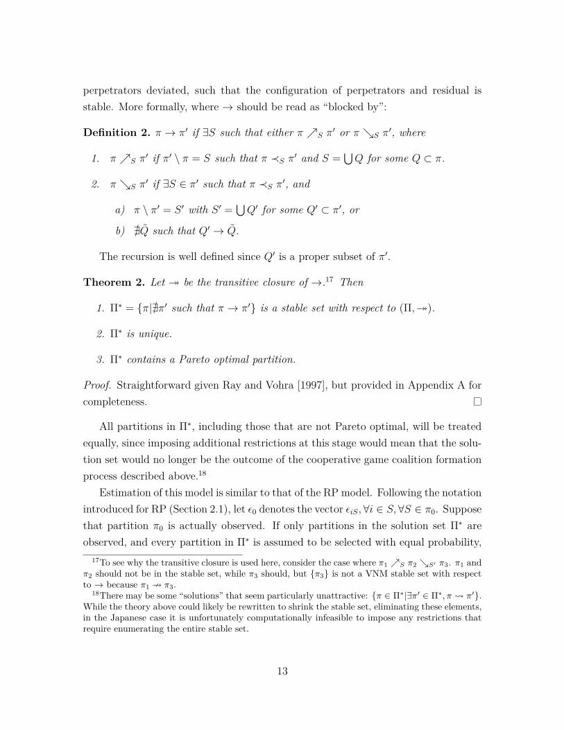
perpetrators deviated, such that the configuration of perpetrators and residual isstable. More formally, where → should be read as “blocked by”:

Definition 2. π → π′ if ∃S such that either π ↗S π′ or π ↘S π′, where

1. π ↗S π′ if π′ \ π = S such that π ≺S π′ and S =∪

Q for some Q ⊂ π.

2. π ↘S π′ if ∃S ∈ π′ such that π ≺S π′, and

a) π \ π′ = S ′ with S ′ =∪Q′ for some Q′ ⊂ π′, or

b) ∄Q such that Q′ → Q.

The recursion is well defined since Q′ is a proper subset of π′.

Theorem 2. Let ↠ be the transitive closure of →.17 Then

1. Π∗ = {π|∄π′ such that π → π′} is a stable set with respect to (Π,↠).

2. Π∗ is unique.

3. Π∗ contains a Pareto optimal partition.

Proof. Straightforward given Ray and Vohra [1997], but provided in Appendix A forcompleteness.

All partitions in Π∗, including those that are not Pareto optimal, will be treatedequally, since imposing additional restrictions at this stage would mean that the solu-tion set would no longer be the outcome of the cooperative game coalition formationprocess described above.18

Estimation of this model is similar to that of the RP model. Following the notationintroduced for RP (Section 2.1), let ϵ0 denotes the vector ϵiS, ∀i ∈ S, ∀S ∈ π0. Supposethat partition π0 is actually observed. If only partitions in the solution set Π∗ areobserved, and every partition in Π∗ is assumed to be selected with equal probability,

17To see why the transitive closure is used here, consider the case where π1 ↗S π2 ↘S′ π3. π1 andπ2 should not be in the stable set, while π3 should, but {π3} is not a VNM stable set with respectto → because π1 ↛ π3.

18There may be some “solutions” that seem particularly unattractive: {π ∈ Π∗|∃π′ ∈ Π∗, π ⇝ π′}.While the theory above could likely be rewritten to shrink the stable set, eliminating these elements,in the Japanese case it is unfortunately computationally infeasible to impose any restrictions thatrequire enumerating the entire stable set.

13

then the parameters θ can be estimated via maximum likelihood. The likelihood ofπ0 occurring is

L(π0|θ) =∫ϵ

I(π0 stable |θ, ϵ)∫ΠI(π stable |θ, ϵ)fπdπ

fϵ(ϵ)dϵ

= P (π0 ∈ Π∗|θ)∫ϵ

1∫ΠI(π stable |θ, ϵ)fπdπ

fϵ(ϵ|π0 ∈ Π∗, θ)dϵ

= P (π0 ∈ Π∗|θ)Eϵ|π0∈Π∗,θ

[1

Z

], (9)

where Z is the number of stable partitions (i.e. |Π∗|). Since the distribution of ϵis known by assumption, this could in theory be calculated exactly. Due to com-putational constraints, however, both terms in the above likelihood function will beestimated. Assume that π0 in fact consists of π0,1, π0,2, ..., π0,K , the outcomes of Kindependent coalition formation games. Then Z = Z1Z2 · · ·ZK , and take the Kthroot of both sides of the above equation. Then

K√L(π0|θ) = K

√P (π0 ∈ Π∗|θ)Eϵ|π0∈Π∗,θ

[1

Z

](10)

is a consistent M-estimator for θ. However, for computational reasons it is not possibleto calculate the above, so instead a numerical approximation of the expectation willbe used. In particular, consider the case where K → ∞. Then

logZ − µπ0,θ√K

∼ N(0, σπ0,θ) (11)

and1

Eϵ|π0∈Π∗,θ[Z]→p Eϵ|π0∈Π∗,θ

[1

Z

]. (12)

Now letEϵ|π0∈Π∗,θ[Z] = |Π|ρπ0,θ, (13)

14

where ρ is the fraction of partitions that are stable.19 ρ will be estimated by randomlyselecting a set of partitions ΠA and calculating the probability that they are stable.This results in the estimator

K

√P (π0 ∈ Π∗|θ) 1

|Π| 1|ΠA|Σπ∈ΠA

P (πi ∈ Π∗|π0 ∈ Π∗, θ)

= K√|Π| K

√P (π0 ∈ Π∗|θ)|ΠA|

Σπ∈ΠAP (πi ∈ Π∗|π0 ∈ Π∗, θ)

. (14)

Since |Π| does not depend on θ, an equivalent estimator is

K

√P (π0 ∈ Π∗|θ)|ΠA|

Σπ∈ΠAP (πi ∈ Π∗|π0 ∈ Π∗, θ)

. (15)

The actual estimation is performed via numerical approximation of the above prob-abilities. Specifically, if E0 is a set of draws from the distribution of ϵ0, then theapproximation is

1

|E0|∑ϵ0∈E0

P (π0 ∈ Π∗|θ, ϵ0)|ΠA|∑

π∈ΠAP (π ∈ Π∗|θ, ϵ0, π0 ∈ Π∗)

. (16)

Once again, because of the convenient error partitioning of the above, the probabilitycan be expanded into a product of independent events. Let S↑

0 be the set of allcoalitions that could be formed by mergers of the coalitions in π0, and let S↓

0 be theset of all coalitions that are a subset of a coalition in π0. Then

P (π0 ∈ Π∗|θ, ϵ0) =∏

S∈(S↑0∪S

↓0 )

P (π0 ⊀S S|θ, ϵ0). (17)

19Interchanging the expectation and reciprocal operations is valid because

E[1

Z] = E[

1

eΣi=K logZi]

= E[e−Σi=Klog Zi

K K ]

= E[e−µK+o( K√

K)]

= E[e−µK+o(√K)]

≃ E[e−µK ],

since µ > 1 because π0 ∈ Π∗.

15

Now approximate the denominator by defining ϵl and El in the same way as ϵ0 andE0:

P (πl ∈ Π∗|θ, ϵ0, π0 ∈ Π∗) =1

|El|∑ϵl∈El

∏S∈(S↑

l ∪S↓l )

P (πl ⊀S S|θ, ϵ0, ϵl, π0 ∈ Π∗). (18)

There are two problems with estimating this numerically. First, draws need to bemade from ϵl|θ, ϵ0, π0 ∈ Π∗, and second, given a draw of ϵl from the correct distribu-tion, the required probability needs to be calculated efficiently. Fortunately, for bothcases, an application of Bayes’ Rule is sufficient. To draw from ϵl|θ, ϵ0, π0 ∈ Π∗, firstdefine ϵS to be the idiosyncratic shocks to coalition S ∈ πl. If S is not a potentialdeviation from π0, then ϵS|θ, ϵ0, π0 ∈ Π∗ = ϵS since no additional information is pro-vided by the fact that π0 is stable. If S is a potential deviation from π0, then considerthe identity

f(ϵS|θ, ϵ0) = f(ϵS|θ, ϵ0, π0 ⊀ S)P (π0 ⊀S S|θ, ϵ0)

+ f(ϵS|θ, ϵ0, π0 ≺S S)P (π0 ≺S S|θ, ϵ0). (19)

Here f(ϵS|θ, ϵ0) is equal to the unconditional density f(ϵS), which is known by assump-tion. The second distribution on the right hand side is a set of truncated distributionsbecause if π0 ≺S S then it must be true that ui(S) > ui(π0), and thus

ϵi > ui(π0)− vi(S), (20)

and these can be calculated sequentially. Thus, the desired distribution can be drawnby simulating from

f(ϵS|θ, ϵ0, π0 ⊀S S) =f(ϵS|θ, ϵ0)− f(ϵS|θ, ϵ0, π0 ≺S S)P (π0 ≺S S|θ, ϵ0)

P (π0 ⊀S S|θ, ϵ0), (21)

which can be done sequentially for each member of S.20

20The simplest way of ensuring that π0 is always in the stable set is to draw a new ϵ for each newproposed θ; however, this introduces simulation “chatter”, making convergence difficult. Instead ofsimulating ϵ0 directly, then, draw quantile indices qj , and create ϵj from qj fresh for each iterationof θ.

16

The next problem is using these drawn ϵl to calculate the probability

P (πl ⊀S S|θ, ϵ0, ϵl, π0 ∈ Π∗) (22)

where S ′ is some coalition not in πl. If S ′ is not a potential deviation from π0, thenthe calculation is identical for those done for π0, described above. However, if S ′

is a potential deviation from π0, then the fact that π0 is stable provides additionalinformation that needs to be taken into account. Consider the following:

P (πl ⊀S′ S ′|θ, ϵ0, ϵl) = P (πl ⊀S′ S ′|θ, ϵ0, ϵl, π0 ⊀ S ′)P (π0 ⊀S′ S ′|θ, ϵ0, ϵl)

+ P (πl ⊀S′ S ′|θ, ϵ0, ϵl, π0 ≺S′ S ′)P (π0 ≺S′ S ′|θ, ϵ0, ϵ1). (23)

Since the left hand side can be calculated and the second term of the right hand sidehas the same set of truncated distributions described just above with respect to theϵl, rearrangement once again permits calculation:

P (πl ⊀S′ S ′|θ, ϵ0, ϵl, π0 ⊀S′ S ′) = (24)1− P (πl ≺S′ S ′|θ, ϵ0, ϵl)− (1− P (πl ≺S′ S ′|θ, ϵ0, ϵl, π0 ≺S′ S ′))P (π0 ≺ S ′|θ, ϵ0, ϵ1)

1− P (π0 ≺S′ S ′|θ, ϵ0, ϵl).

Everything on the right hand side of this equation can be computed quickly, makingoptimization feasible.

3 ApplicationTreating municipal mergers as a pure hedonic coalition formation problem is con-sistent with anecdotal evidence concerning how mergers are effected. Negotiationsregarding compensation seem to be rare, even though controversy is common andthe results of unrest sometimes significant.21 Some of the involved municipalitiesmay be in favour of a proposed merger while others may be opposed, but those infavour do not seem to promise large transfers to those opposed in order to secure theircooperation. This suggests that there is some problem with contractibility in polit-

21For example, in Canada the merger of all municipalities on Montreal Island in 2002 was a majorcause of the provincial government losing the next election, and the demerger process following thatelection meant that on net only limited change occurred despite significant economic and politicalcosts.

17

ical mergers such that transfers are difficult or impossible, and thus it seems moreplausible to model mergers as a coalition formation game without transfers. First,a model of jurisdictions with heterogeneity in individual ideal points is presented, inthe style of Greenberg and Weber [1986], Demange [1994], and in particular Alesinaand Spolaore [1997]. The Japanese data used is then described, and parameters areestimated via the methods presented in the preceding section.

3.1 Municipal Public Goods Model

Suppose that each municipality m provides a public good of quality qm at a cost ofqm · c(Pm), where P is population, and c exhibits economies of scale. The municipal-ity levies taxes at rate τm and receives transfers Tm from the national government.Population is distributed on a plane, and the public good is provided at a singlephysical location xm on this plane. Suppose that there is some minimum tolerablelevel of public good provision q. Individual utility will be assumed to be additivelyseparable:

ui(qm, τm, θm) = β0 log((1− τm)yi) + β1 log(qm − q) + β2ℓi(θm) + ϵim (25)

where ℓi is the distance between individual i and location of the public good, withβ2 < 0. The error term ϵ is irrelevant until the possibility of mergers is considered.The location of the public good is a multidimensional political decision, a problemwhich has no generally accepted solution concept. However, if this decision is madeby a single elected official, such as a mayor, and voting in elections is determined viaa probabilistic voting model where vote probabilities are linear in utility differencebetween two candidates, then the policy chosen will in fact be the socially optimalpolicy [Banks and Duggan, 2005].22 In this case, this will set θm to the location ofthe generalized median voter.

The optimal quality supplied is determined by the budget constraint τmYm =

qmc(Pm)− Tm, where Ym is total income of all individuals in the municipality, which22Prior to the merger period, mayors were responsible for delivering hundreds of “agency delegated

functions” from higher levels of government, making them bureaucrats as well as politicians, andmaking it possible (at least in theory) for central ministries to fire a mayor for not performing adelegated function according to specifications. “Agency delegated functions” were abolished duringthe merger period, and municipal policies are thus modeled as being determined by local residentsthrough a political process.

18

leads to

q∗m = β1

Ym + Tm − qc(Pm)

c(Pm)+ q (26)

τ ∗m = 1− β0

Ym + Tm − qc(Pm)

Ym

, (27)

if β0 + β1 = 1. Due to the functional form assumption all individuals prefer τ ∗m

regardless of income, and thus this is the tax rate implemented.In this model, individuals do not move or otherwise change their ideal point and

population is assumed to be constant. In reality, residence choice is endogenousto government characteristics, as discussed in the literature established by Tiebout[1956] and others. This endogeneity is not included in this paper for three reasons.First, mobility is lower in Japan than in most other developed countries and a largeportion of the inter-municipality moves reported in the census appear to be temporary.Endogenous relocation is thus less of a concern than in other countries. Second, thereis no evidence of tax competition. The majority of municipalities charge a standardtax rate and even though municipalities are allowed to set a different rate (within aband), few choose to exercise this option. This is consistent with the model presentedabove, and combined with the national government transfer scheme results in theendogeneity problem being less severe than it would be in other contexts. Finally,from an implementation perspective, endogeneity would result in future populationand other characteristics of a municipal merger depending on what other mergersoccurred in the surrounding area. This would change the nature of the coalitionformation game from a characteristic function game to a partition function game,which is substantially more computationally intensive to estimate, and likely infeasiblewithout further theoretical or technological developments. Population dynamics arethus ignored, with the estimates that follow focusing on a single period game withplayer characteristics determined based on current government data sources.23

19

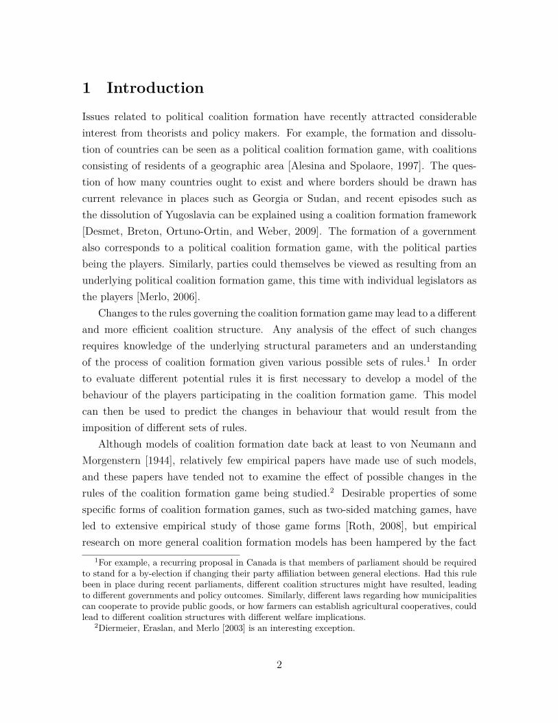
Figure 1: Shizuoka Prefecture

0 0.1 0.20.05Decimal Degrees

4Shizuoka Prefecture

1995 borders

2006 borders

3.2 Data

There were 3,255 municipalities in 1999 at the start of the merger period, divided into47 prefectures (similar to U.S. states). Since mergers do not cross prefectural bound-aries, each prefecture is treated as a separate coalition formation game.24 Figure 1shows the mergers that occurred in Shizuoka Prefecture. Mergers were voluntary, andneeded to be approved by the municipal council of every participating municipality.25

23Similar results were obtained when 2005 census data is used instead of the 1995 data currentlyused. Predicted future municipal population could be created based on census data, but the simi-larity of results obtained with data from different census years suggests that this exercise may notproduce particularly interesting results.

24There is one exception, involving a single municipality switching prefectures. It is treated asthough the municipality in question was always part of the “destination” prefecture.

25In about a third of cases, referenda were held. Nominally, these were consultative, but thereis only one instance in which a municipal council voted opposite to a referendum result. This casewas complicated due to multiple referenda with conflicting results as well as a number of of otherprocedural irregularities, and finally resulted in a recall of the mayor and a request to the prefecturalgovernor to reverse the merger. The request for reversal was denied.

20

The involvement of the municipal council suggests that some form of legislative bar-gaining model may be needed; however this paper abstracts away from this issue andsupposes that a single elected official such as the mayor is responsible for decision-making. In the simplified framework presented here, these decisions will be optimalfrom the perspective of municipal residents, and parameters to the utility functiongiven in Equation 25 can thus be estimated by examining the mergers that actuallyoccurred.26

The number of municipalities dropped to 1,750 in 2010, due to 598 mergers rangingin size from two municipalities up to fifteen municipalities. These mergers occurredmainly due to changes to the rules determining transfers T . Historically, transferswere determined by the formula

Tm = max(cm(Pm)− .75τYm, 0), (28)

where cm is the estimated cost to the municipality of providing those services (referredto as “Standard Fiscal Need” in official documents), and τ a reference tax rate set bythe national government. Here the scale for quality has been normalized such that the“national minimum” level of quality used by the government to compute StandardFiscal Need is 1. Although there were provisions for municipalities to merge, therewas little incentive for them to do so, because if a coalition S decided to form a new(amalgamated) municipality, TS would be calculated exactly as in Equation 28:

TS = max(cS(PS)− .75τYS, 0). (29)

Thus almost all savings would be passed to the national government, and even aslight preference for smaller jurisdictions ensured that residents would be opposed tomergers.27

During the fiscal difficulties of the early 1990s, the national government imple-mented a series of reforms designed to reduce the total transfers provided to munic-ipalities while attempting to minimize the negative effects of this decrease. Thesereforms consisted mainly of a lump sum cut in transfers to all municipalities, making

26The possibility of future mergers is ruled out. Given that the previous set of municipal mergersoccurred in the 1960s, experience suggests that any future mergers are likely far enough away thata reasonable discount rate reduces their importance to the point where they can safely be ignored.

27In general, the division of a municipality was prohibited. In one case, such a split did occur,but both of the resulting municipalities were immediately merged with different neighbours.

21

it difficult for small municipalities to maintain service quality unless they merged,and change to Equation 29 to reduce the penalty associated with merging.

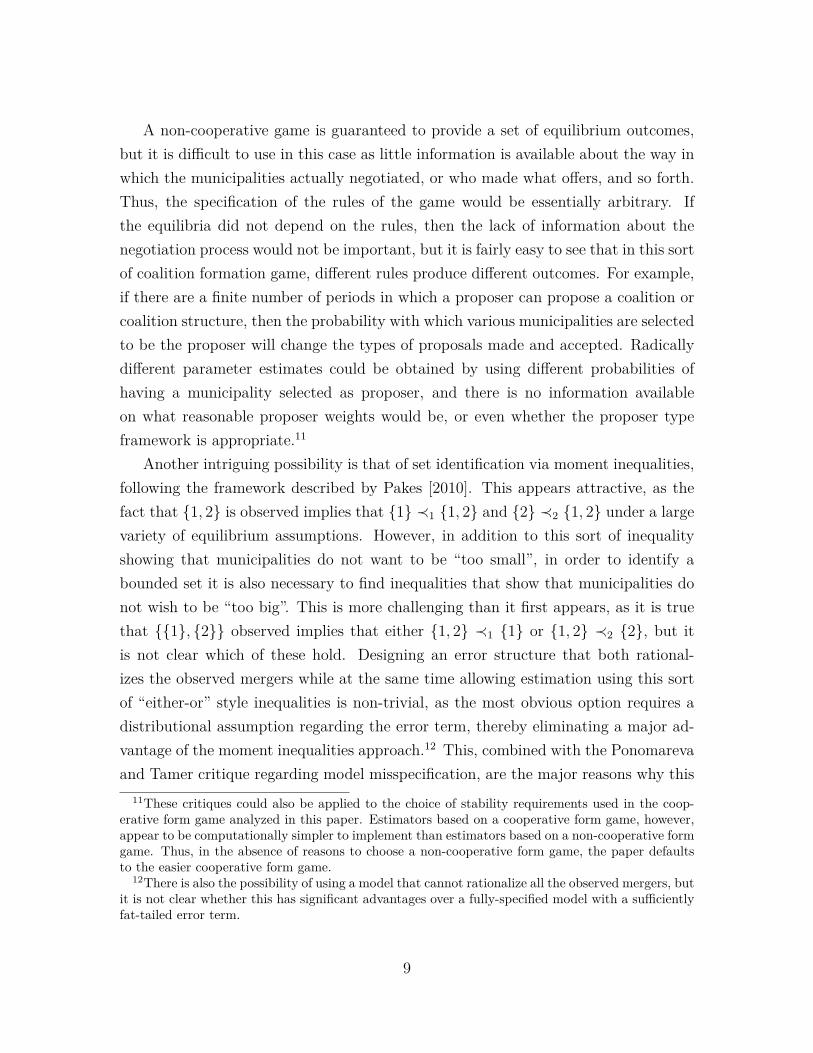
Data sources for municipal population, income per capita, etc. are described inAppendix B. Details regarding c and the changes to the transfer formula are given inAppendix C. Further general information on the Japanese local public finance systemavailable from Mochida [2008]. Hayashi, Nishikawa, and Weese [2010] examine theissues surrounding c in some detail and conclude that c ≃ c: that is, the nationalgovernment estimates accurately reflect the actual efficiencies of scale in the provisionof public services.28 These efficiencies of scale are substantial, as shown in Figure 2(see Appendix C for details).

A final interesting feature of municipal finance in Japan is that there is littlevariation in tax rates charged by municipalities: despite the fact that local govern-ments have the authority to choose any rate within a band established by the nationalgovernment, almost all charge τm = τ . One possible explanation is political: munic-ipalities charge τ even though τ > τ ∗m for most m because of pressure from higherlevels of government or the risk of negative publicity. This is unsatisfying in thatit suggests that a much more complicated model, one involving political processesabout which little is known, is necessary in order to explain the observed municipaltax system. Another possibility is to set q = 1, that is, to make the official nationalminimum standard the boundary between intolerably low and acceptable levels ofpublic services for individuals. This is also unsatisfying in that it implies that anylevel of government service below the national minimum would result in infinite disu-tility; however, it has the major advantage that Equation 27 reduces to

τ ∗m = 1− β0(1− .75τ)

for municipalities that are receiving transfers, using Equation 28 and the assumptionthat cm = cm. Therefore, τ ∗m = τ if β0 = 1−τ

1−.75τ, which is about 0.97 when τ = 0.12,

28To briefly summarize Hayashi et al. [2010], over-representation of rural areas within the JapaneseDiet means that the risk is that government estimates overstate efficiencies of scale, rather thanunderstating them. If the true efficiencies of scale were lower than the government estimates shownin Figure 2, then smaller municipalities were receiving rents. If such rents existed, then either theywere distributed to residents, which should be visible in land prices, or they were captured by a groupof political insiders, which should result in rural political leaders being more opposed to municipalmergers than their constituents; however, neither of these phenomena are observed.

22

Figure 2: Standard Fiscal Need

Population (1000s of residents)

¥100

,000

s pe

r ca

pita

1

5

10

1 10 100 1000

the observed average tax rate. Although this value for β0 is higher than the estimatedvalue discussed later (β0 = 0.91), bootstrap analysis suggests that the null hypothesisthat β0 =

1−τ1−.75τ

should not be rejected. The assumption that q = 1 will thus be usedboth for estimation and the analysis of counterfactual policies.

3.3 Estimation

Consider Equation 25, but simplify and replace municipality m with coalition S:

ui(qS, τS, θS) = β0 log(1− τS) + β1 log(qS − q) + β2ℓi(θS) + ϵiS. (30)

23

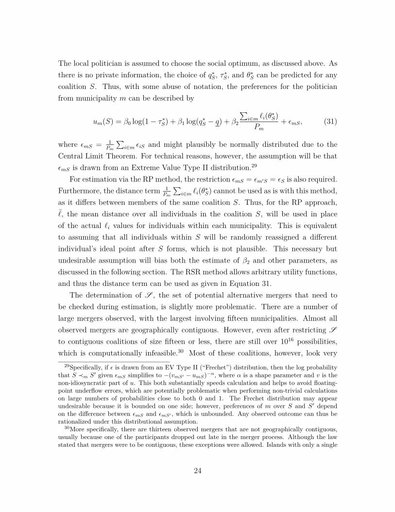
The local politician is assumed to choose the social optimum, as discussed above. Asthere is no private information, the choice of q∗S, τ ∗S, and θ∗S can be predicted for anycoalition S. Thus, with some abuse of notation, the preferences for the politicianfrom municipality m can be described by

um(S) = β0 log(1− τ ∗S) + β1 log(q∗S − q) + β2

∑i∈m ℓi(θ

∗S)

Pm

+ ϵmS, (31)

where ϵmS = 1Pm

∑i∈m ϵiS and might plausibly be normally distributed due to the

Central Limit Theorem. For technical reasons, however, the assumption will be thatϵmS is drawn from an Extreme Value Type II distribution.29

For estimation via the RP method, the restriction ϵmS = ϵm′S = ϵS is also required.Furthermore, the distance term 1

Pm

∑i∈m ℓi(θ

∗S) cannot be used as is with this method,

as it differs between members of the same coalition S. Thus, for the RP approach,ℓ, the mean distance over all individuals in the coalition S, will be used in placeof the actual ℓi values for individuals within each municipality. This is equivalentto assuming that all individuals within S will be randomly reassigned a differentindividual’s ideal point after S forms, which is not plausible. This necessary butundesirable assumption will bias both the estimate of β2 and other parameters, asdiscussed in the following section. The RSR method allows arbitrary utility functions,and thus the distance term can be used as given in Equation 31.

The determination of S , the set of potential alternative mergers that need tobe checked during estimation, is slightly more problematic. There are a number oflarge mergers observed, with the largest involving fifteen municipalities. Almost allobserved mergers are geographically contiguous. However, even after restricting S

to contiguous coalitions of size fifteen or less, there are still over 1016 possibilities,which is computationally infeasible.30 Most of these coalitions, however, look very

29Specifically, if ϵ is drawn from an EV Type II (“Frechet”) distribution, then the log probabilitythat S ≺m S′ given ϵmS simplifies to −(vmS′ − umS)

−α, where α is a shape parameter and v is thenon-idiosyncratic part of u. This both substantially speeds calculation and helps to avoid floating-point underflow errors, which are potentially problematic when performing non-trivial calculationson large numbers of probabilities close to both 0 and 1. The Frechet distribution may appearundesirable because it is bounded on one side; however, preferences of m over S and S′ dependon the difference between ϵmS and ϵmS′ , which is unbounded. Any observed outcome can thus berationalized under this distributional assumption.

30More specifically, there are thirteen observed mergers that are not geographically contiguous,usually because one of the participants dropped out late in the merger process. Although the lawstated that mergers were to be contiguous, these exceptions were allowed. Islands with only a single

24

different than the actually observed coalitions. In particular, they tend to be a thinline of municipalities, stretching almost all the way across a prefecture. On average,individuals in these coalitions would have very high distance ℓ, and the coalitions arethus not likely to form. Including this group of “low probability” coalitions in thecalculations would be ideal. However, for computational reasons these will insteadbe ruled out through the use of a restriction: coalitions will not be allowed to crossmore than two county boundaries, using county definitions from the Meiji era.31

This restriction dramatically reduces the number of large coalitions that need to beconsidered: with fifteen-municipality coalitions, only one coalition in a billion involvesthree or fewer counties.32 This reduces the total number of alternatives that need tobe considered to about 20 million per prefecture, which is computationally feasible.

Another problem that is only relevant to the estimation via RSR is the estimationof the size of the stable set. Since the number of partitions grows exponentially withthe number of municipalities, it is not possible to examine all partitions. The totalnumber of partitions is unknown but bounded above by the Bell numbers (Sloane#A000110), which are greater than 10100 for larger prefectures such as Hokkaidō.Therefore, a random sample is drawn instead. It is, however, non-trivial to randomlysample from a set which is too large to be enumerated. Thus, random draws areobtained using Markov chains, as described in Appendix D.

3.4 Results

The results are shown in Table 1, with scale determined by the restriction β0+β1 = 1

and standard errors approximated via likelihood ratio tests. Columns I and II are

municipality on them are treated as being connected to the closest municipality on the “mainland”(i.e. Hokkaidō, Honshū, Shikoku, or Kyūshū) if it is within 50km. There are, however, two cases inwhich municipalities on an island merged with municipalities on the mainland other than the closestone. There are also six cases where municipalities on two separate islands merged together. Thus,about 3.5% of mergers (21/588) are not contiguous. No additional mergers violating contiguity aregenerated as comparison coalitions, although the mergers did occur are retained in the observedpartitions, and may also appear in alternative partitions.

31In particular, the county boundaries used are from 1878 for eastern Japan, and 1896 for westernJapan. Counties are statistical divisions, and have not had any political function since the 1920s.Counties in Tokyo and Nagano Prefectures are anomalously large, and thus in those prefectures onlythe restriction is to one and two counties, respectively, rather than three.

32Two actual mergers violate the restriction on number of counties that is imposed: one sizetwelve merger in Shizuoka, and one size eleven merger in Niigata. This represents 0.3% of allobserved mergers.

25

Table 1: Dependent variable is um(S), utility to municipality m from merger S

relaxed stability requirements restricted preferencesI II III IV

CONSUMPTION (β0) 0.909 0.913 1.014 1.020(0.074) (0.098) (0.120) (0.127)

GOVERNMENT (β1) 0.091 0.087 −0.014 −0.020(0.002) (0.005) (0.001) (0.001)

DISTANCE (10 · β2) −0.086 −0.072 −0.035 −0.039(0.001) (0.003) (0.001) (0.001)

DISTANCE_POL −0.068 0.015(0.024) (0.006)

scale 1.955 0.210 0.152 0.275shape 107.569 16.281 9.150 14.880N (prefectures) 46 46 40 40

estimates using the RSR approach, while columns III and IV are estimates using theRP approach. Columns I and III use exactly the utility function discussed previ-ously, while Columns II and IV include one additional variable: DISTANCE_POLis the average political distance to the new median voter on a one dimensional polit-ical spectrum, using political spectrum location estimates from Kubo, Mitsuyo, andKishimoto [2006]. Results obtained via the RSR approach are consistent with theory:higher private (post-tax) consumption and better government services are desirable,while greater distance, both geographic and on the political spectrum, is undesirable.

Assuming that income and transfers per capita are identical across all municipal-ities, and ignoring the effect of the transfer scheme on merger incentives, the ratioof the coefficients regarding geographic distance and government services in ColumnI of Table 1 imply that a municipality would be willing to accept an increase in av-erage distance between residents’ ideal points and policy location of 10km (disutilityof 0.086), in exchange for decreasing the per capita cost of providing governmentservices by a factor of e (utility of 0.091). From the perspective of private consump-tion, an individual with average income is willing to accept about ¥25,000 per yearin exchange for an increase in distance of 1km. This estimate may seem high; how-ever, municipalities are responsible for public school facilities, and municipal mergersare often followed by school amalgamations. For many families, travel to the public

26

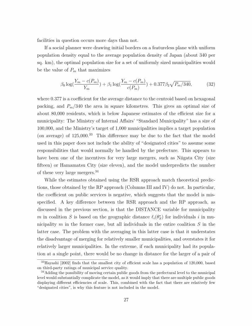
facilities in question occurs more days than not.If a social planner were drawing initial borders on a featureless plane with uniform

population density equal to the average population density of Japan (about 340 persq. km), the optimal population size for a set of uniformly sized municipalities wouldbe the value of Pm that maximizes

β0 log(Ym − c(Pm)

Ym

) + β1 log(Ym − c(Pm)

c(Pm)) + 0.377β2

√Pm/340, (32)

where 0.377 is a coefficient for the average distance to the centroid based on hexagonalpacking, and Pm/340 the area in square kilometres. This gives an optimal size ofabout 80,000 residents, which is below Japanese estimates of the efficient size for amunicipality: The Ministry of Internal Affairs’ “Standard Municipality” has a size of100,000, and the Ministry’s target of 1,000 municipalities implies a target population(on average) of 125,000.33 This difference may be due to the fact that the modelused in this paper does not include the ability of “designated cities” to assume someresponsibilities that would normally be handled by the prefecture. This appears tohave been one of the incentives for very large mergers, such as Niigata City (sizefifteen) or Hamamatsu City (size eleven), and the model underpredicts the numberof these very large mergers.34

While the estimates obtained using the RSR approach match theoretical predic-tions, those obtained by the RP approach (Columns III and IV) do not. In particular,the coefficient on public services is negative, which suggests that the model is mis-specified. A key difference between the RSR approach and the RP approach, asdiscussed in the previous section, is that the DISTANCE variable for municipalitym in coalition S is based on the geographic distance ℓi(θ

∗S) for individuals i in mu-

nicipality m in the former case, but all individuals in the entire coalition S in thelatter case. The problem with the averaging in this latter case is that it understatesthe disadvantage of merging for relatively smaller municipalities, and overstates it forrelatively larger municipalities. In the extreme, if each municipality had its popula-tion at a single point, there would be no change in distance for the larger of a pair of

33Hayashi [2002] finds that the smallest city of efficient scale has a population of 120,000, basedon third-party ratings of municipal service quality.

34Adding the possibility of moving certain public goods from the prefectural level to the municipallevel would substantially complicate the model, as it would imply that there are multiple public goodsdisplaying different efficiencies of scale. This, combined with the fact that there are relatively few“designated cities”, is why this feature is not included in the model.

27

Table 2: Monte Carlo simulations (median estimate and 95% interval)

true relaxed stability requirements restrictedvalue (rest. dist.) preferencesI II III IV

CONSUMPTION (β0) 0.913 0.908 0.970 1.010[0.245, 0.981] [0.820, 0.995] [1.003, 1.019]

GOVERNMENT (β1) 0.087 0.092 0.030 −0.010[0.019, 0.755] [0.005, 0.180] [-0.019, -0.003]

DISTANCE (10 · β2) −0.072 −0.067 −0.027 −0.015[-0.497, -0.017] [-0.119, -0.011] [-0.033, -0.010]

DISTANCE_POL −0.068 −0.067 −0.012 −0.010[-0.448, -0.008] [-0.088, 0.013] [-0.038, 0.020]

scale 0.210 0.204 0.055 0.093shape 16.281N (pref. per rep.) 15R (replications) 100

municipalities if they merged, as the location of the generalized median voter wouldremain unchanged. An inaccurately low estimate of the value of government servicescounteracts this effect, as the change in the quality of government services is largerfor the smaller municipalities participating in a merger than for the larger ones.

Table 2 shows this effect with artificial data created from the parameter valuesshown in Column I, which correspond to those in Column II of Table 1, and arebased on the RSR model. Column II of Table 2 verifies that these parameters canbe recovered with acceptable finite sample bias and simulation noise via the strategypresented in this paper. Column IV of Table 2 shows that if this simulated datais used to estimate parameters based on the RP model, a negative coefficient ongovernment services is obtained, as in Columns III and IV of Table 1. Column III ofTable 2 shows results obtained by running the RSR model using the modified distancedata necessary to meet the restrictions of the RP model. The parameter estimatesin Column III are closer to those of Column IV than Column II, showing that themajority of the bias in the estimates in Column IV is due to the different definitionof distance that must be used, rather than the different distributional assumption

28

inherent in the model.35 For the counterfactual policy simulations presented below,then, the RSR model will be treated as the correct model.

A major advantage of having coefficient estimates for a structural model is theability to conduct counterfactual analysis. Two alternative national government poli-cies can be examined: first, national government enforcement of transfers negotiatedbetween municipalities during the coalition formation process; second, an incentivescheme for richer municipalities that participate in mergers.

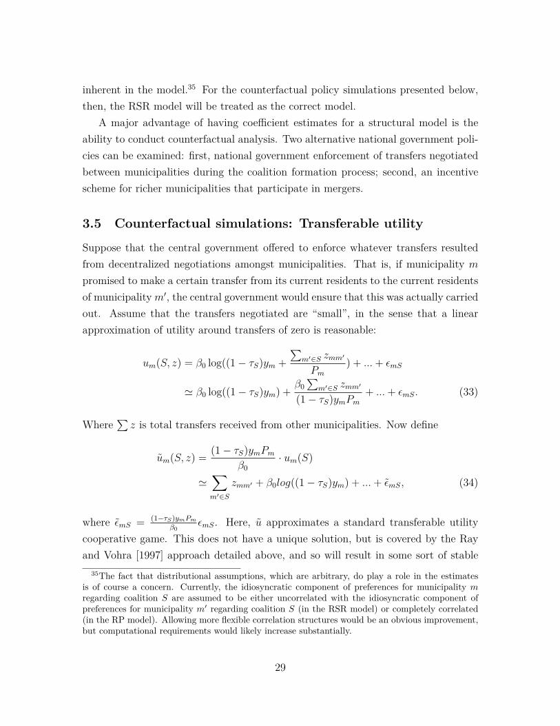
3.5 Counterfactual simulations: Transferable utility

Suppose that the central government offered to enforce whatever transfers resultedfrom decentralized negotiations amongst municipalities. That is, if municipality m

promised to make a certain transfer from its current residents to the current residentsof municipalitym′, the central government would ensure that this was actually carriedout. Assume that the transfers negotiated are “small”, in the sense that a linearapproximation of utility around transfers of zero is reasonable:

um(S, z) = β0 log((1− τS)ym +

∑m′∈S zmm′

Pm

) + ...+ ϵmS

≃ β0 log((1− τS)ym) +β0

∑m′∈S zmm′

(1− τS)ymPm

+ ...+ ϵmS. (33)

Where∑

z is total transfers received from other municipalities. Now define

um(S, z) =(1− τS)ymPm

β0

· um(S)

≃∑m′∈S

zmm′ + β0log((1− τS)ym) + ...+ ϵmS, (34)

where ϵmS = (1−τS)ymPm

β0ϵmS. Here, u approximates a standard transferable utility

cooperative game. This does not have a unique solution, but is covered by the Rayand Vohra [1997] approach detailed above, and so will result in some sort of stable

35The fact that distributional assumptions, which are arbitrary, do play a role in the estimatesis of course a concern. Currently, the idiosyncratic component of preferences for municipality mregarding coalition S are assumed to be either uncorrelated with the idiosyncratic component ofpreferences for municipality m′ regarding coalition S (in the RSR model) or completely correlated(in the RP model). Allowing more flexible correlation structures would be an obvious improvement,but computational requirements would likely increase substantially.

29

Figure 3:

25 30 35 40 45 50

−0.

020.

000.

020.

040.

06

Income.per.capita

Util

ity.c

hang

e

set. If random ϵ are drawn, then some idea of the efficiency gain of enforcing theTU game, versus simply administering a fixed incentive structure, can be obtained.The exact transfers, however, depend on which stable coalition structure forms andexactly how the surplus from each coalition is divided. For a given coalition S, thepossible utilities of the municipalities are determined by the possible values of x,where the following conditions are satisfied:

1.∑

m∈S xm = V (S), and

2.∑

m∈S′ xm ≥ V (S ′) ∀S ′ ⊂ S,

where V (S) =∑

m∈S u(S) is the value of coalition S.It seems extremely unlikely that poor municipalities would have more bargaining

power than rich municipalities, and thus an “equitable” distribution of the surplusseems to be the most optimistic scenario. A more pessimistic scenario would givemost of the bargaining power to richer municipalities, with a resulting increase inpost-merger inequality.

30

The nucleolus is used as a “best case” equitable division: it is the allocation whichmaximizes over all potential deviating coalitions S ′ the smallest difference betweenthe amount allocated to the members of S ′ and that which they could obtain if theydeviated.36 To estimate the utility obtained in this case, 100 separate draws of ϵwere performed for the eight smallest prefectures, and the resulting nucleoli wereaveraged. This was compared to the no-transfer case, using the same 100 draws ofϵ. The results are shown graphically in Figure 3. Municipalities with a per capitaincome of less than ¥3,500,000 (about 18% of total population) are worse off, relativeto the no-transfers case, while richer municipalities are much better off. Thus, makingtransfers feasible may or may not be optimal for the national government, dependingon its social welfare function. A worst-case scenario was also examined, where richermunicipalities are assumed to have all of the bargaining power, and thus as muchsurplus as possible is transferred to the richest municipality, and then the next richest.The results are very similar to those shown in Figure 3, although the regressive natureof the transfers is slightly more pronounced.

3.6 Counterfactual simulations: Incentives to merge

If transfers between players are disallowed or otherwise impossible, but there is asocial planner that can provide incentives for coalition formation, then at least in thetwo player case, the social planner should offer such incentives:

Example 3. In the setup described in Example 1, if ϵ1 and ϵ2 are random variableswith density f , then before the ϵ are known, ∃τ, δ > 0 such that both players would bein favour of a social planner offering an incentive δ for coalition formation:

ui({1}) = ui({1})− τ

ui({1, 2}) = ui({1}) + ϵi + δ

E[1(u1({1, 2}) > u1({1})) · 1(u2({1, 2}) > u2({2})) · δ] = τ (35)36More specifically, x is determined by argmin

xmaxS′⊂S E(S′), where E(S′) is the excess of coali-

tion S′: E(S′) = V (S′)−∑

m∈S′ xm. Note that if S is part of a stable partition, E(S′) < 0 ∀S′ ⊂ S.There may be more than one x that leads to the same maximum above, but by continuing to mini-mize excesses lexicographically, a unique value of x is obtained.

31

Ex ante, both players are in favour of this incentive being offered because

E[ui] = E[ui({i})] (36)+ E[1(u1({1, 2}) > u1({1})) · 1(u2({1, 2}) > u2({2})) · (ui({1, 2})− ui({i}))]

and thus

∂E[ui]

∂δ|δ=0 = f(0)(E[max(ui({1, 2}), ui({i}))]− ui({i})) > 0 (37)

Intuitively, the gains from the incentive are first order, occurring whenever oneplayer is almost indifferent between forming the {1,2} coalition or not, and the otherplayer is very much in favour. The losses, on the other hand, are second order: whenboth players are almost indifferent, the incentive results in a {1,2} coalition nowforming when it wouldn’t have previously. In a game with more than two players,however, any new coalition that forms due to this sort of incentive might displace anexisting non-singleton coalition, thus changing the set of stable coalition structures.This is an additional cost of offering the incentive, and any general theorem regardingthe efficiency of offering incentives to form (non-singleton) coalitions would have tohave restrictions to ensure that the cost of such a disruption of existing coalitions isnot too high. The definition of “too high” in this case would depend on the socialwelfare function used, but a simulation shows that welfare improving policies do existfor reasonable social welfare functions.

In particular, suppose that the national government offered an additional, budgetbalanced incentive for certain municipalities to merge. The targeted municipalitiesshould be those that are most likely to be opposed to mergers that would benefitother municipalities, and the most likely municipalities to fall into that category arericher municipalities. Consider the policy that offered a transfer equivalent to 0.3%of income, to residents of richer municipalities that participated in a merger, where a“richer” municipality is defined as one that had income per capita above the averagefor the merger that they are participating in. This transfer would be paid for by anincrease in the income tax on everyone.

To determine the effects of such a policy, stable partitions are simulated underboth the actual and the proposed alternative policies.37 The difference between the

37These partitions are produced by generating random coarsenings of an all-singleton partition

32

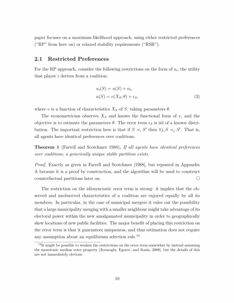
Figure 4:Utility change from incentive scheme

Income per capita

U(w

ith in

cent

ives

) −

U(o

rigin

al p

olic

y)

−0.02

0.00

0.02

25 30 35 40 45 50

actual and alternative policies are shown in Figure 4.38 In addition to increasingutility overall, the increase is the same for poorer and richer municipalities. Thisis in contrast to the case with negotiated transfers, where poorer municipalities sawdecreased utility. For some set of inequality-averse social welfare functions, a socialplanner might choose not to allow municipalities to negotiate transfers, but mightinstead set a fixed incentive scheme, one that rewarded desirable municipalities formerging with their neighbours. Such an incentive scheme, however, suffers from theproblem that it appears to be regressive, in that it taxes everyone in order to maketransfers to the rich, and thus might be infeasible for political reasons.

and then drawing from this set of partitions after all the duplicates have been removed. This isa consistent method of drawing a sample of stable partitions with uniform selection probability,although it is biased (i.e. the probability of selection is not uniform) when the random coarseningsdrawn do not enumerate all the stable partitions. The degree of bias depends on the numberof random coarsenings drawn, but this bias does not appear to be important, since changing thenumber of random coarsenings generated does not change the results.

38The regression line shown is weighted by municipal population.

33

4 ConclusionThis paper estimated the parameters determining preferences in a cooperative formpolitical coalition formation game, using two different sets of assumptions and defi-nitions of the solution set. The results obtained via the RSR approach are consistentwith intuition, while some coefficient estimates obtained via the RP approach areimplausible. This difference is due mainly to the fact that preferences over coalitionsdiffer by player, and this can be incorporated within the RSR approach. The pa-rameters estimated via the RSR approach are used to examine potential alternativenational government policies. Counterfactual simulations suggest that an alternativeincentive scheme that rewarded relatively rich municipalities for merging would haveresulted in welfare improvements under most reasonable social welfare functions. Al-lowing transfers to be negotiated between municipalities may or may not be superior,depending on the national government’s aversion to inequality and the bargainingpower of the various municipalities. The latter is likely unknown to the nationalgovernment, and thus even if transfers between municipalities could be enforced, itmay not be beneficial for the national government to do so.39 At least as importantas the implications to government policy, however, is the methodology developed.A coalition formation game without transfers accurately describes many real-worldphenomena, but it is rarely estimated in the empirical literature. As the price ofcomputing power decreases, however, the number of uses of this sort of model thatare feasible should increase. Although the game presented in this paper could beestimated only because the geographical nature of the data permitted a large numberof possible coalitions to be discarded, such restrictions are less likely to be necessaryin the future. The results given above, then, are hopefully only an early indication ofthe applications of this type of coalition formation model.

39One possibility that was not considered in this paper is that of a tax on negotiated transfers.In the simplest price control model, a tax redistributed to the consumer should be able to mimic aprice control, but with the assurance that the consumers with the highest willingness to pay obtainthe good. To the extent that the inability to make transfers is like a price control at zero, then, itcould be that the optimal policy for the government – rather than specifying a fixed incentive schemeto encourage rich municipalities to merge with their neighbours – would be to allow transfers, buttax them heavily and redistribute the revenue obtained to the poorest municipalities. Overall, theproblem bears some resemblance to the classic rent control problem.

34

ReferencesDaron Acemoglu. Why not a political coase theorem? social conflict, commitment,and politics. Journal of Comparative Economics, 31(4):620–652, December 2003.

Daron Acemoglu, Georgy Egorov, and Konstantin Sonin. Dynamics and stability ofconstitutions, coalitions, and clubs. Technical report, NBER, August 2008.

Alberto Alesina and Enrico Spolaore. On the number and size of nations. TheQuarterly Journal of Economics, 112(4):1027–1056, November 1997.

Alberto Alesina, Reza Baqir, and Caroline Hoxby. Political jurisdictions in hetero-geneous communities. The Journal of Political Economy, 112(2):348–396, April2004.

Mark Armstrong and John Vickers. A model of delegated project choice. Economet-rica, 78(1):213–244, 2010.

Suryapratim Banerjee, Hideo Konishi, and Tayfun Sönmez. Core in a simple coalitionformation game. Social Choice and Welfare, 18(1):135–153, January 2001.

Jeffrey Banks and John Duggan. Probabilistic voting in the spatial model of elections:The theory of office-motivated candidates. In David Austen-Smith and John Dug-gan, editors, Social Choice and Strategic Decisions, Studies in Choice and Welfare,pages 15–56. Springer Berlin Heidelberg, 2005.

S. Barberà and A. Gerber. A note on the impossibility of a satisfactory concept ofstability for coalition formation games. Economics Letters, 95(1):85–90, April 2007.

Anna Bogomolnaia and Matthew O. Jackson. The stability of hedonic coalition struc-tures. Games and Economic Behavior, 38(2):201–230, February 2002.

David M. Brasington. Joint provision of public goods: the consolidation of schooldistricts. Journal of Public Economics, 73(3):373–393, 1999.

B. Dahlby and L.S. Wilson. Fiscal capacity, tax effort, and optimal equalizationgrants. The Canadian Journal of Economics, 27(3):657–672, 1994.

Gabrielle Demange. Intermediate preferences and stable coalition structures. Journalof Mathematical Economics, 23(1):45–58, January 1994. ISSN 0304-4068.

Klaus Desmet, Michel Le Breton, Ignacio Ortuno-Ortin, and Shlomo Weber. Thestability and breakup of nations: A quantitative analysis. SSRN eLibrary, June2009.

Effrosyni Diamantoudi and Licun Xue. Coalitions, agreements and efficiency. Journalof Economic Theory, 136(1):105–125, September 2007.

35

Daniel Diermeier, Hulya Eraslan, and Antonio Merlo. A structural model of govern-ment formation. Econometrica, 71(1):27–70, 2003.

J. H. Dreze and J. Greenberg. Hedonic coalitions: Optimality and stability. Econo-metrica, 48(4):987–1003, May 1980.

Joseph Farrell and Suzanne Scotchmer. Partnerships. The Quarterly Journal ofEconomics, 103(2):279–297, May 1988.

Frank Flatters, Vernon Henderson, and Peter Mieszkowski. Public goods, efficiency,and regional fiscal equalization. Journal of Public Economics, 3(2):99–112, May1974.

Jeremy T. Fox. Estimating matching games with transfers. Technical report, NBER,October 2008.

D. Gale and L. S. Shapley. College admissions and the stability of marriage. TheAmerican Mathematical Monthly, 69(1):9–15, January 1962.

Nora Gordon and Brian Knight. A spatial merger estimator with an application toschool district consolidation. Journal of Public Economics, 93(5-6):752–765, June2009.

Joseph Greenberg. Stability when mobility is restricted by the existing coalitionstructure. Journal of Economic Theory, 21(2):213–221, October 1979.

Joseph Greenberg and Shlomo Weber. Strong tiebout equilibrium under restrictedpreferences domain. Journal of Economic Theory, 38(1):101–117, February 1986.

Masayoshi Hayashi. Congestion, technical returns and the minimum efficient scalesof local government expenditures: The case of japanese municipalities. TechnicalReport 01-01, Institute for Research in Bus. and Econ., Meiji Gakuin, 2002.

Masayoshi Hayashi, Masashi Nishikawa, and Eric Weese. Inefficient municipal bound-aries. Technical report, Aoyama Gakuin, 2010. [In Japanese].

Nobuo Ishihara. Shin Chihou Zaisei Chousei Seido Ron. Gyousei, Tokyo, new edition,2000. [”New Local Finance Regulation System”].

Hideki Kido and Etsuhiro Nakamura. Strategy and environment: Determinants ofmunicipal amalgamations. Annals of the Japanese Society for Public Administra-tion, 43:112–130, 2008. [In Japanese].

Takahiro Kubo, Yamamoto Mitsuyo, and Kazuo Kishimoto. Estimating the downsianlocations of parties from the numbers of votes gained by the parties. Transactions ofthe Japan Society for Industrial and Applied Mathematics, 16(4):563–574, December2006. [In Japanese].

36

Antonio Merlo. Whither political economy? theories, facts and issues. In RichardBlundell, Whitney K Newey, and Torsten Persson, editors, Advances in Economicsand Econometrics: Theory and Applications, Ninth World Congress, number 41 inEconometric Society monographs. Cambridge University Press, Cambridge, 2006.

Thomas J. Miceli. The decision to regionalize in the provision of education: Anapplication of the tiebout model. Journal of Urban Economics, 33(3):344–360,May 1993.

Nobuki Mochida. Fiscal Decentralization and Local Public Finance in Japan. Number107 in Routledge frontiers of political economy. Routledge, London, 2008.

John Von Neumann and Oskar Morgenstern. Theory of Games and Economic Be-havior. Princeton university press, Princeton, 1944.

A. Pakes. Alternative models for moment inequalities. Econometrica, 78(6):1783–1822, 2010.

Dale J. Poirier. Partial observability in bivariate probit models. Journal of Econo-metrics, 12(2):209–217, February 1980.

Maria Ponomareva and Elie Tamer. Misspecification in moment inequality models:Back to moment equalities? Econometrics Journal. forthcoming.

Debraj Ray and Rajiv Vohra. Equilibrium binding agreements,. Journal of EconomicTheory, 73(1):30–78, March 1997.

Christian P Robert and George Casella. Monte Carlo Statistical Methods. Springertexts in statistics. Springer, New York, 2nd ed edition, 2004.

Alvin Roth. Deferred acceptance algorithms: history, theory, practice, and openquestions. International Journal of Game Theory, 36(3):537–569, March 2008.

T. Saarimaa and J. Tukiainen. Coalition formation and political decision making.Technical report, Government Institute for Economic Research, Finland, 2010.

Charles M. Tiebout. A pure theory of local expenditures. The Journal of PoliticalEconomy, 64(5):416–424, October 1956.

Kenneth E Train. Simulation methods for probit and related models based on con-venient error partitioning. Technical Report 95-237, UC Berkeley, 1995.

Eric Weese. Political mergers as coalition formation : Evidence from japanese mu-nicipal amalgamations. Technical report, Center for Research on ContemporaryEconomic Systems, Hitotsubashi University, December 2008.

S. Wernicke. Efficient detection of network motifs. Computational Biology and Bioin-formatics, IEEE/ACM Transactions on, 3(4):347–359, 2006.

37

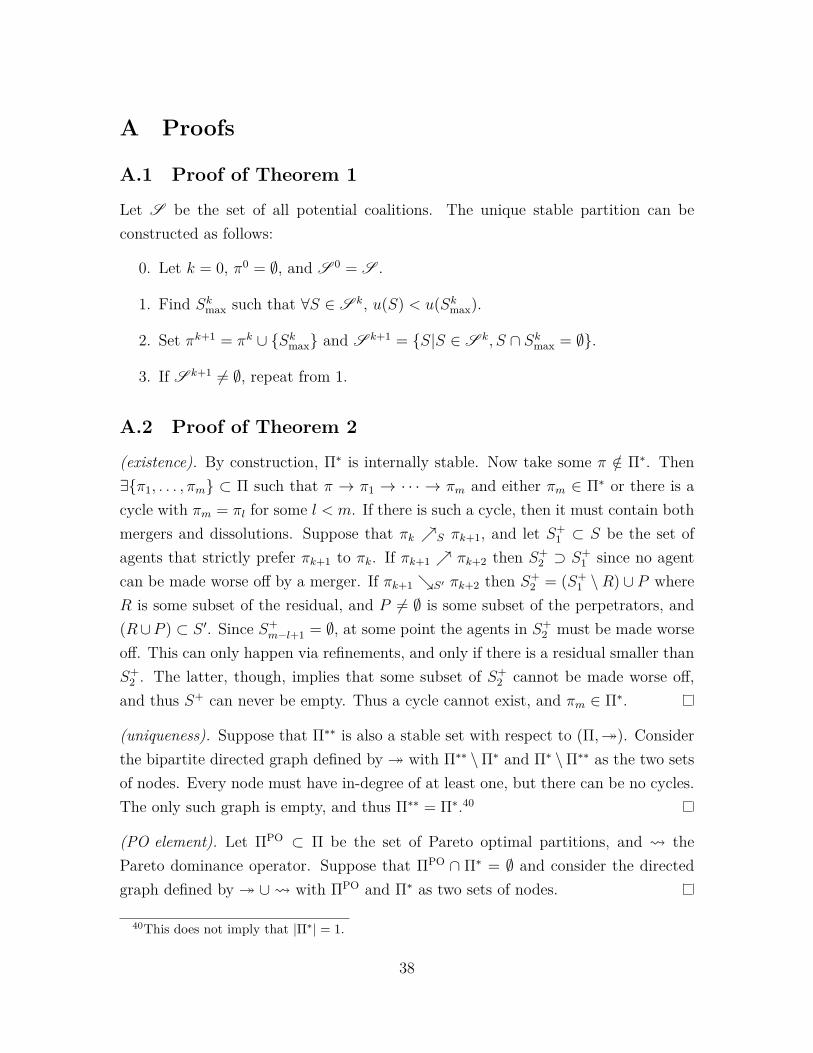
A Proofs

A.1 Proof of Theorem 1

Let S be the set of all potential coalitions. The unique stable partition can beconstructed as follows:

0. Let k = 0, π0 = ∅, and S 0 = S .

1. Find Skmax such that ∀S ∈ S k, u(S) < u(Sk

max).

2. Set πk+1 = πk ∪ {Skmax} and S k+1 = {S|S ∈ S k, S ∩ Sk

max = ∅}.

3. If S k+1 = ∅, repeat from 1.

A.2 Proof of Theorem 2

(existence). By construction, Π∗ is internally stable. Now take some π /∈ Π∗. Then∃{π1, . . . , πm} ⊂ Π such that π → π1 → · · · → πm and either πm ∈ Π∗ or there is acycle with πm = πl for some l < m. If there is such a cycle, then it must contain bothmergers and dissolutions. Suppose that πk ↗S πk+1, and let S+

1 ⊂ S be the set ofagents that strictly prefer πk+1 to πk. If πk+1 ↗ πk+2 then S+

2 ⊃ S+1 since no agent

can be made worse off by a merger. If πk+1 ↘S′ πk+2 then S+2 = (S+

1 \R) ∪ P whereR is some subset of the residual, and P = ∅ is some subset of the perpetrators, and(R∪P ) ⊂ S ′. Since S+

m−l+1 = ∅, at some point the agents in S+2 must be made worse

off. This can only happen via refinements, and only if there is a residual smaller thanS+2 . The latter, though, implies that some subset of S+

2 cannot be made worse off,and thus S+ can never be empty. Thus a cycle cannot exist, and πm ∈ Π∗.

(uniqueness). Suppose that Π∗∗ is also a stable set with respect to (Π,↠). Considerthe bipartite directed graph defined by ↠ with Π∗∗ \Π∗ and Π∗ \Π∗∗ as the two setsof nodes. Every node must have in-degree of at least one, but there can be no cycles.The only such graph is empty, and thus Π∗∗ = Π∗.40

(PO element). Let ΠPO ⊂ Π be the set of Pareto optimal partitions, and ⇝ thePareto dominance operator. Suppose that ΠPO ∩ Π∗ = ∅ and consider the directedgraph defined by ↠ ∪⇝ with ΠPO and Π∗ as two sets of nodes.

40This does not imply that |Π∗| = 1.

38

B DataPopulation data comes from the 1995 national census, which provides data at thekilometer grid square level. Taxable income per capita is used as a proxy for incomeper capita, with 1996 tax year data taken from the Asahi Shimbun Minryoku. Thelist of mergers that actually occurred is from the Japan Geographic Data Center. Toconstruct the set of possible coalitions information on which municipalities share aborder is derived from shape files for 1995 boundaries from ESRI Japan. These filesare also used in conjunction with the census grid square data to calculate the locationof generalized median voters.41

Municipal financial data is from the ’96-’97 and (for comparison) the ’06-’07 fiscalyear Shichōsonbetsu Kessan Jōkyō Shirabe, an official national government reportof municipal finances.42 Because of the large transfers from the national treasuryto local governments, this data is handled quite carefully by officials in the centralministries and is generally regarded as accurate, particularly the sections producedby the central government itself. The isolated incidents of fraud reported generallyrelate to variables reported by the municipalities, which are not used in this paper.

Table 3 gives summary statistics for this data. Units for population and surfacearea are chosen to be close to the Ministry of Internal Affairs’ “reference municipality”.There are no missing values in any of the financial, population, or surface area data.In the income data, four values are missing because one merger took place after thedata was collected but before it was published, and the old municipalities were notreported. This variable, however, is only used in the preliminary financial regressionsdescribed below, and thus the data used in the main estimator does not have anymissing values.43

41A precise calculation of the generalized median is computationally intensive, and infeasible giventhe number of such values that need to be computed. A simple calculation of median latitude andmedian longitude, however, yields a good approximation, and is used throughout the paper. Usingthe mean voter, which is easy to calculate but not consistent with the model presented, yields similarresults.

42This report also provides by municipality population data from the 1995 census, and surfacearea data from a 1996 Geographical Survey Institute survey.

43The 23 “special wards”, which cover roughly the area of pre-war Tokyo City, have powers similarto cities but are excluded from the analysis because any enlargement of this sui generis area wouldlikely involve adding more wards, rather than changing the borders of existing ones. The twelve“designated cities”, which have some powers normally reserved for prefectures, are omitted fromthe preliminary financial calculations because their additional responsibilities increase their requiredspending, but they are included in the rest of the analysis as regular cities. The categories of “core

39

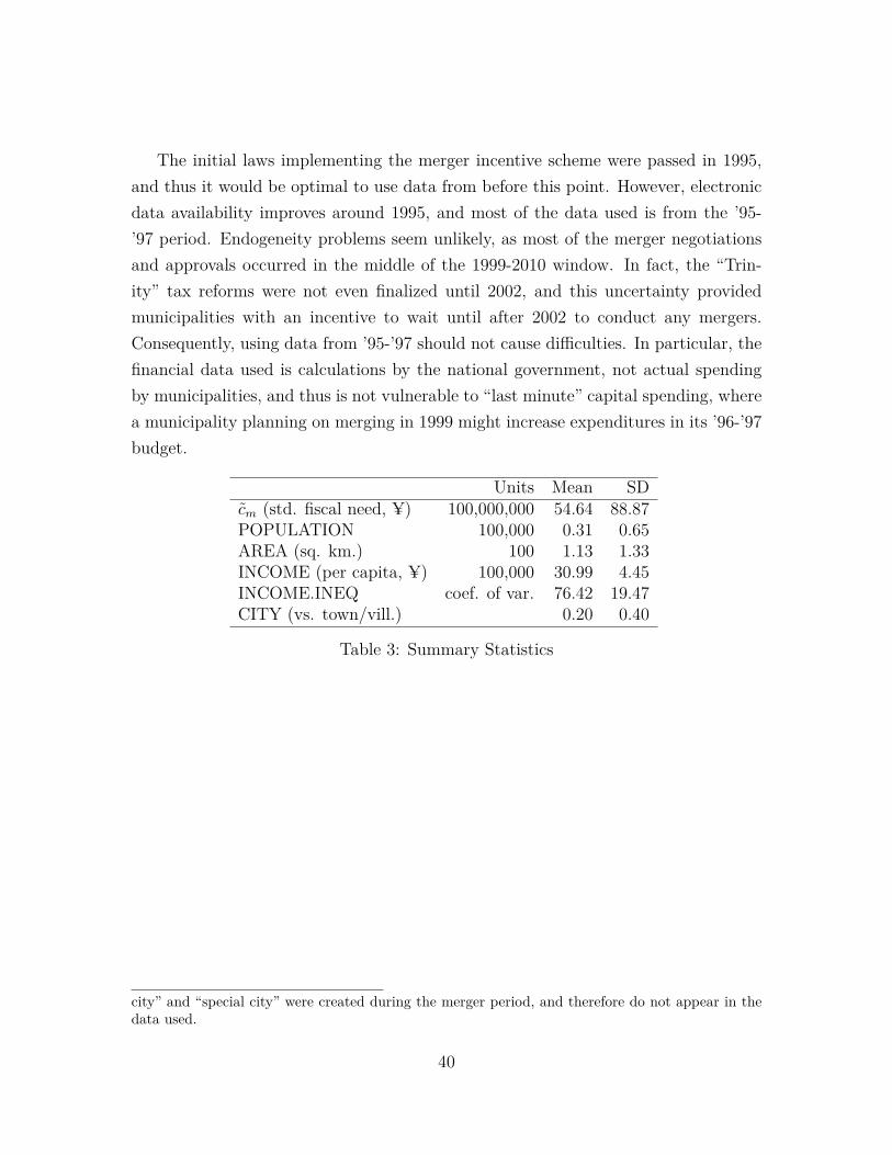
The initial laws implementing the merger incentive scheme were passed in 1995,and thus it would be optimal to use data from before this point. However, electronicdata availability improves around 1995, and most of the data used is from the ’95-’97 period. Endogeneity problems seem unlikely, as most of the merger negotiationsand approvals occurred in the middle of the 1999-2010 window. In fact, the “Trin-ity” tax reforms were not even finalized until 2002, and this uncertainty providedmunicipalities with an incentive to wait until after 2002 to conduct any mergers.Consequently, using data from ’95-’97 should not cause difficulties. In particular, thefinancial data used is calculations by the national government, not actual spendingby municipalities, and thus is not vulnerable to “last minute” capital spending, wherea municipality planning on merging in 1999 might increase expenditures in its ’96-’97budget.

Units Mean SDcm (std. fiscal need, ¥) 100,000,000 54.64 88.87POPULATION 100,000 0.31 0.65AREA (sq. km.) 100 1.13 1.33INCOME (per capita, ¥) 100,000 30.99 4.45INCOME.INEQ coef. of var. 76.42 19.47CITY (vs. town/vill.) 0.20 0.40

Table 3: Summary Statistics

city” and “special city” were created during the merger period, and therefore do not appear in thedata used.

40

C Japanese Local Public FinancePost-war Japanese fiscal policy emphasized equalization between municipalities, andestablished national standards for local government services.44 To ensure that ev-ery municipality had sufficient funds to offer services above this minimum level, thenational government developed a complicated system of transfers, called the “LocalAllocation Tax”.45 The estimated cost cm for the provision of public services variesfrom municipality to municipality, based on a formula developed by bureaucrats atthe Ministry of Internal Affairs and Communications. The 2009 version of the ex-position of this formula (the Chihō Kōfuzei Seido Kaisetsu) consists of 600 pages ofJapanese legal text, 460 pages of formulae, and 240 pages of reference values; however,as Figure 2 shows, cm can be approximated by the non-linear regression

cm(Pm) = (γ0 + γ1Pθm)vm, (38)

where vm is a lognormal error term.46 The fixed cost is thus γ0, and the averagevariable cost is γ1P θ−1

m . The values in Table 4 reflect the fact that the central ministriesbelieved that there were economies of scale in the production of public goods, andthus per capita costs would be higher in municipalities with lower population: thefixed cost estimate is about ¥600 million for Columns II-V, and the marginal cost(γ1θP θ−1

m ) is about ¥200,000 per capita at a population of 1,000, but ¥100,000 per44One possible reason for this policy would be to correct a Flatters, Henderson, and Mieszkowski

[1974] “fiscal externality”; however, this requires the possibility of migration between municipalities,which is not included in this paper. Dahlby and Wilson [1994] provide an alternative explanationthat is consistent with the model in this paper, where the goal of the transfer scheme is equalizingthe marginal cost of public funds across municipalities.

45The slightly-confusing name is due to the fact that it is an allocation to local governments fromtaxes collected by the national government.

46The underprediction for large municipalities in Figure 2 is not necessarily evidence that Equation38 is misspecified. Although “designated cities” have been removed, large cities that do not quitemeet the criteria to be so designated appear to have been allocated some additional responsibilitieson a more ad hoc basis. Because the underlying data that the Standard Fiscal Need calculationsare based on is not available, the amount allocated for these additional responsibilities is difficultto remove; however, Hayashi et al. [2010] show that the functional form used here matches costestimates generated by the dankai hosei adjustment coefficient, which is the adjustment that createsmost of the per capita cost difference between municipalities with large and small populations. Weese[2008] used a simpler specification which matched the data in Figure 2 better for large municipalities:this specification was changed to that in Equation 38 after consulting with the Ministry of InternalAffairs officials responsible for the cost estimates.

41

I II III IV V(Intercept) 9.57∗ 5.67∗ 6.15∗ 5.94∗ 6.16∗

(0.19) (0.12) (0.17) (0.12) (0.17)θ 0.90∗ 0.90∗ 0.87∗ 0.93∗ 0.89∗

(0.01) (0.00) (0.01) (0.01) (0.01)

POPULATIONθ 137.19∗ 139.17∗ 143.01∗ 146.76∗ 145.21∗

(2.89) (3.04) (3.14) (3.02) (3.01)AREA 3.19∗ 2.73∗ 3.13∗ 2.58∗

(0.10) (0.10) (0.10) (0.09)INCOME 0.01 0.09∗ −0.03 −0.00

(0.02) (0.03) (0.03) (0.03)INCOME.INEQ −0.07∗ −0.07∗ −0.03∗ −0.04∗

(0.00) (0.01) (0.01) (0.01)

POPθ*INCOME 1.02∗ 2.11∗

(0.25) (0.27)

POPθ*INCOME.INEQ −0.60∗ −0.81∗

(0.07) (0.07)PREFECTURE N N Y N YCITY N N Y N YN 3220 3216 3216 3216 3216

Table 4: Dependent variable is Standard Fiscal Need (’96-’97)

capita at a population of 100,000.47 Taking into account both the fixed cost and thevariable cost, the per capita cost of providing national minimum level public goodsin Ashiyasu village (population 567) would be roughly ¥1.5 million, compared withroughly ¥100,000 in Sakai city (population 790,000).

With almost half of pre-merger municipalities having a population less than 10,000,the decision to provide additional subsidies to smaller municipalities due to their sizewas an expensive one. To attempt to reduce this inefficiency, in the 1990s the gov-ernment implemented three policies designed to promote mergers.

First, the government substantially reduced transfers to the smallest municipalities47Column I is provided for reference, but as there are explicit expense categories dealing with land

administration (particularly forests and farmland), surface area is an obvious variable to include.The results in Column I show that the null hypothesis that there are no economies of scope betweenadministering land and providing services to residents cannot be rejected: the difference in estimatesfor γ1 and θ are both statistically insignificant between Column I and Column II. Comparisons withColumns III-V do yield some statistically significant differences, but using parameter values fromthese columns does not change the results in the following sections of the paper.

42

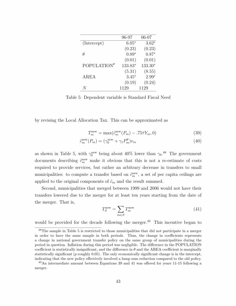
96-97 06-07(Intercept) 6.05∗ 3.62∗

(0.23) (0.23)θ 0.89∗ 0.87∗

(0.01) (0.01)

POPULATIONθ 133.83∗ 133.30∗

(5.31) (8.55)AREA 3.45∗ 2.99∗

(0.19) (0.24)N 1129 1129

Table 5: Dependent variable is Standard Fiscal Need

by revising the Local Allocation Tax. This can be approximated as

T newm = max(cnew

m (Pm)− .75τYm, 0) (39)cnewm (Pm) = (γnew

0 + γ1Pθm)vm (40)

as shown in Table 5, with γnew0 being about 40% lower than γ0.48 The government

documents describing cnewm make it obvious that this is not a re-estimate of costs

required to provide services, but rather an arbitrary decrease in transfers to smallmunicipalities: to compute a transfer based on cnew

m , a set of per capita ceilings areapplied to the original components of cm and the result summed.

Second, municipalities that merged between 1999 and 2006 would not have theirtransfers lowered due to the merger for at least ten years starting from the date ofthe merger. That is,

T newS =

∑m∈S

T newm (41)

would be provided for the decade following the merger.49 This incentive began to48The sample in Table 5 is restricted to those municipalities that did not participate in a merger

in order to have the same sample in both periods. Thus, the change in coefficients representsa change in national government transfer policy on the same group of municipalities during theperiod in question. Inflation during this period was negligible. The difference in the POPULATIONcoefficient is statistically insignificant, and the difference in θ and the AREA coefficient is marginallystatistically significant (p roughly 0.05). The only economically significant change is in the intercept,indicating that the new policy effectively involved a lump sum reduction compared to the old policy.

49An intermediate amount between Equations 39 and 41 was offered for years 11-15 following amerger.

43

be phased out in 2006, which motivated many municipalities to finalize mergers in2005. By 2006 there were only 1,844 municipalities remaining, down from 3,255 at thestart of the merger period. A small number of mergers occurred during the phase-outperiod, reducing the final number of municipalities to 1,750 in 2010; for the purposesof this paper, these mergers are treated as though they were finalized prior to 2006,and implementation was simply delayed for exogenous reasons.50

A final incentive for mergers was the Gappei Tokureisai, special subsidized bondissues allowed for municipalities planning amalgamation.51 The value of these bondsis calculated based on the subsidy offered, using information from Ishihara [2000].Municipalities are presumed to able to save in order to equalize the quality of publicservices and the municipal tax rate between the decade immediately following themerger, when incentives are provided, and following decades.

50Explaining why a coalition would not form during the 1999-2005 period, but would under theprogressively less-advantageous policies in place in 2006-2010 would require adding elements to themodel, such as arrival of new information, that would substantially complicate the analysis. Thismay be an interesting area for further work.

51The official explanation for these bonds was to eliminate any direct financial cost of merging,such as the construction of a new city hall. The merger bonds appeared to allow significant capitalexpenditures beyond the actual costs of amalgamation. Relative to the incentive provided by theswitch from cm to cnewm in the calculation of transfers, these bonds have a very small effect onincentives to merge, and thus for simplicity the the bonds are treated entirely as an additionalincentive, with the direct financial costs of merging ignored.

44

D Random Draws of Partitions via Markov ChainsLet the state space X be the set of all partitions, and the transition matrix P bedefined as follows:

Pxy = k if y can be created by either breaking apart one coalition in x intosubcoalitions, or merging coalitions in x together to create one new coalition,

Pxy = 0 ∀y = x that do not meet the above condition,Pxx = 1−

∑y =x Pxy.

Since the state space is finite, this creates a valid transition matrix for sufficientlysmall k. P describes a reversible Markov chain, since a transition from x to y viamerging implies a possible transition from y to x via a breakup, and vice versa. Thechain is connected, since any partition can be obtained by first breaking all coali-tions down to singletons, and then constructing the desired partition. There is thus aunique stationary distribution, since the chain satisfies the detailed balance condition[Robert and Casella, 2004]. Moreover, the stationary distribution gives equal prob-ability to each state, and thus draws from the stationary distribution are equivalentto random draws from the set of all partitions. These draws can be performed usingthe Metropolis-Hastings algorithm.

Unfortunately, the number of transitions that need to be considered is too largeto be computationally feasible. The number of ways a size fifteen coalition couldbe broken down into sub coalitions could be as high as a billion, and thus it is notpractical to enumerate all the possible transitions. Instead, the approach introducedby Wernicke [2006] for the RAND-ESU algorithm will be used. Let p be a lengthfifteen vector of “cut probabilities” and let Q be a set of subcoalitions of S that forma partition of S. Then enumerate a member of Q with probability

∏i∈{1,...,|S|} pi.

This gives each member of Q an equal probability of being enumerated, but allowsfor a much smaller, randomly selected set to be considered. So long as this randomlyselected Q is re-randomized each time a given state is reached, then the properties ofthe above Markov chain are unchanged.

45