A Long Introduction to Economic Theory and Natural Gas

Ferdinand E. Banks* Abstract This paper has its origin in a long lecture that I gave at the ENI Corporate University in Milan, Italy, which I later extended for the natural gas portion of the course in oil and gas economics that I taught in 2007 at the Asian Institute of Technology, Bangkok (Thailand). What I attempt now is to utilize the discussions of gas in my two energy economics textbooks (2000, 2007), plus various short and long articles, to present a more up-to-date survey of world gas, as well as to provide serious readers with a ‘competitive advantage’ in their interaction with students, teachers, and/or colleagues. On the basis of my familiarity with the learned and popular literature, I believe that there is an inadequate supply of energy economics surveys, which is why this contribution seems appropriate. The topics considered here include energy units and heat equivalents, gas reserves and production theory, pipelines, price issues, storage, Russian gas, liquefied natural gas, and the deregulation of natural gas. The last section begins with comments on two widely discussed ‘sets’ of pipelines, one from Alaska toward the US, and one from e.g Russia toward ‘West Europe’. Keywords: Gas reserves and output, merit order, Russian gas, deregulation, pipelines.

1. INTRODUCTION

“Energy is the go of things,” as James Clerk Maxwell pointed out many years ago. Put another way, no energy no go!

Once this is clear, the next step is to obtain an unambiguous quantitative description of some aspects of that “go”. This is where courses in energy economics often disappoint their participants, because many teachers of these courses make a point of ignoring or downgrading the most useful elements of the subject. My students however are very seldom in danger of experiencing unpleasant surprises in routine discussions with other students or for that matter energy professionals, because I inform them early in my first lecture that it in their interest to keep me convinced that they have a satisfactory knowledge of topics like those presented in the present paper.

Before commencing a systematic examination of this topic, something should be made clear. According to Robert Bryce, managing editor of the Energy Tribune Magazine, coal dominated the energy picture in the 19th century, oil the 20th, and – in his opinion – natural gas will be the dominant “fuel” of the 21st century.

This gives the impression that gas will ‘outshine’ nuclear as, e.g. a source of electricity, which is very dubious. It is now possible to construct a nuclear facility in slightly less than 4 years, where this means 4 years from ‘ground break’ to first grid power, and this reactor should have a ‘life’ of at least 70 years. Given that it does not release any carbon, and its fuel can be reprocessed, it is difficult to believe that nuclear based power will be dominated by a

* Professor Department of Economics, The University of Uppsala, Uppsala Sweden.

fossil fuel (e.g. natural gas) whose global output could peak before the middle of this century. The relation between the very important annual capital cost ‘A’ – or annual payment at the end of each year for T years for an asset costing P0 (which is the investment cost) – can be calculated using the annuity formula. That simple expression is derived in this paper’s appendix, and is:

A=

−+

+1)1(

)1(T

T

rrr

P0 (1)

If any of my students, on any level, anywhere, desire a passing grade, then they are

advised to be able to reproduce and discuss the use of (1) at any hour of the day or night. For instance, if an asset costs $1000 (=P0), T = 2 (years), and we have a discount (e.g. interest) rate of r = 10% , then a simple calculation gives annual payments A. From (1) these are {[r(1+r)T]/[(1+r)T – 1 ]}P0 = {[0.10(1 + 0.10)2]/[(1 + 0.10)2 – 1]}1000 = $576. Moreover, for theoretical purposes, there is no difference between paying $1000 for the asset now, or 1000(1+0.1)2 = $1210 after two years, or $576 at the end of each of the next two years, taking care to remember that theory is one thing and practice another, because payment schedules depend on more than theoretical considerations. T is sometimes called the amortization period, and readers can easily show – formally or otherwise – that an increase in T will bring about a decrease in A.

Thus a nuclear plant with a life of 70 years has a different cost (and profit) outlook from one of 30 years. Why the reference to profit? The answer is that when the cost of other energy resources escalate (due e.g. to depletion), the increased cost of electricity generated from uranium and/or thorium should not be excessive.

2. ENERGY UNITS AND HEAT EQUIVALENTS

In the most elementary, yet most comprehensive sense, energy can be defined as anything that makes it possible to do work – i.e. bring about movement against resistance. Energy takes many forms, and one of its most interesting characteristics is that all aspects of motion, all physical processes, involve to one degree or another the conversion of energy from one state to another. For example, the chemical energy that is found in natural gas can be converted to active heat, which in combination with water will generate steam in a boiler. This steam can then be used to drive a turbine which, in turn, rotates the shaft of an electric generator, and thus produces electricity. Note that the rotating shaft implies the ability to do physical work. For instance, it could be used to turn a merry-go-round or a water wheel, or perhaps to pull a cable car up Coogee Bay Road in the eastern suburb of Sydney (Australia), although, admittedly, these are probably very uneconomical applications. Analogously, the chemical energy in food can be transformed into mechanical energy – i.e. the ability to do physical work – or, if a person is so inclined, the ability to do mental work.

All this is perfectly straightforward, but unfortunately heat cannot be converted into work without loss, and the loss is always in the form of heat at a temperature closer to that of the surroundings than the heat source that made the work possible. Once heat has descended to the ambient (i.e. surrounding) temperature, it is no longer available to do useful work. What we are dealing with here is a highly abstract concept from thermodynamics known as entropy, sometimes called “time’s arrow” , which signifies energy going down the thermal hill and being diffused into space. Lost forever we might say, which implies that the Universe itself is in danger of ‘running down’.

The next thing you need to recall is that one metric ton (= 1 tonne = 1t) equals 2,205 pounds, and that 2.2 pounds = 1 kilogram. (Similarly, 1 inch = 2.54 centimetres, 12 inches =

1 foot, 100 centimetres = 1 meter and thus 1 meter is approximately equal to 3.28 feet = 39.37 inches). In everyday life the usual ton is the short ton, or simply ton, which equals 2,000 pounds. Thus 1t = 1.103 tons.

When dealing with energy we are often interested in heat equivalents, and when the topic is gas the most favoured unit is the British thermal unit, or Btu, which is the amount of heat required to increase the temperature of one pound of water by 1 degree Fahrenheit. (1 pound of water is approximately equal to one pint.) Here it might also be useful to remind readers that with F Fahrenheit, and C Centigrade, we go from C to F with the equation F = (9/5)C +32. In scientific work, and in certain countries, joules can be preferred to the Btu as a unit as a unit of heat energy, however since the price of natural gas is commonly given in dollars per Btu (= $/Btu), there is no point in energy economics to spend a great deal of time pondering the utility of the joule or for that matter the calorie or kilocalorie (= 1000 calories), which are other heat units.

That brings us to a key calculation. 1000 cubic feet (= 1000 cf = 1000 ft3) of natural gas has an approximate energy content of 1,000,000 Btu. (To be exact, 1 ft3 of natural gas has an average heating value of 1035 Btu, but 1000 Btu is almost always used. Moreover, the average energy content of natural gas varies from a low of 845 British Thermal Units per cubic foot (845 Btu/cf = 845 Btu/ft3) in Holland to 1300 Btu/ft3 in Ecuador.) Now let us make a calculation involving gas and crude oil, where one barrel (= 1 b) of oil has an average energy content of 5,686,470 Btu. Today the price of oil is approximately $120/b, and the price of natural gas almost $8 per million Btu, and so it is almost a no-brainer to compare the Btu prices of these two energy resources. The cost of a million Btu of oil is thus 120/5.686 = $21.104 (as compared to $8 for gas). There is a considerable difference between these two prices, and it has been suggested that this difference signifies that the (dollar) price of oil will fall by a great deal.

My position is the opposite: I believe that the gas price will rise, though not to an extent that there will be a Btu equality with oil. This is because oil is a more ‘efficient’ resource than gas, and to a considerable extent easier to deliver and use. But even so the ‘spot’ price of some gas in Asia was recently $20/mBtu, and so that particular price might soon be greater than the listed Btu price of oil. The spot price is the price for immediate (or nearly immediate) delivery, as compared to a forward or term price.

A few more numbers might be in order. 1000 ft3 is equal to 28.3 cubic meters, since 1 cubic meter = 35.3147 cubic feet. The most popular unit for measuring both the production and consumption of oil is millions of barrels per day (mb/d), but instead of barrels per day we sometimes see tonnes per year (= t/y). To derive the equivalency here we need to know that approximately 7.33 barrels of crude oil ‘enclose’ one tonne of crude, and it turns out that barrels/day can be transformed to million tonnes per year (= mt/y) by multiplying by 50. We obtain this important number from a simple dimensional analysis, in which the key operation is cancellation.

≈

year

tonnesbarreltonnesx

yeardaysx

daybarrels 50

33.71365

3. NATURAL GAS RESERVES AND LOCATION In many respects, natural gas is an ideal fuel. Its environmental qualities (in terms of its ‘comparatively’ modest emissions of ‘greenhouse’ gases) have occasionally caused it to be labelled a premium fossil fuel (as compared to oil and coal), and there is a great deal of it in the crust of the earth – though perhaps not as much as many observers believe. As pointed out by Ken Chew (2003), the amount of gas resources discovered annually peaked in the

beginning of the l970s, and the number of discoveries early in the l980s. (This lends weight to a contention by Julian Darley (2004) that gas production could ‘plateau’ before 2025.) Natural gas is found in appreciable quantities in very many countries, with Russia having the world’s largest reserves and in addition being the biggest producer, while the United States (US) is the largest consumer, although it has only about 3% of world reserves. Europe (excluding Russia and Eurasia) consumes roughly 20% of global output. Considerable gas has attained the status of ‘stranded gas’, which means gas that has been discovered but is not economically viable for physical or economic reasons: for instance, it is too far from main pipeline routes, or localities where gas consumption is high, to make its exploitation attractive.

Since l980 natural gas has exhibited the fastest consumption growth of all fossil fuels – averaging between 2.5 percent per year (= 2.5%/y) and 3%/y. Gas is mainly used for heating and cooking, power generation, providing energy for industrial processes, and as a feedstock for fertilizers, chemicals and plastics. Where e.g. power generation is concerned, gas functions as a primary energy input, while the electricity being generated is a secondary energy resource. (Primary energy is energy obtained from the direct burning of coal, gas, and oil, as well as electricity having a hydro or nuclear origin. To these five add wood and waste, geothermal energy, solar thermal, wind and photovoltaic electricity, although they provide only a small fraction in modern societies. Here you should also be aware of the difference between energy – which above is in Btu – and power, which is relevant later in the discussion of compressors for gas pipelines.)

In considering fertilizers in the US, the escalating price of gas – from $2 per thousand Btu in 1999 to a spike of $13 per thousand Btu in July 2008 was the worst possible news for the fertilizer industry, and resulted in the closure of considerable fertilizer production capacity. This outcome was predicted years ago by the Nobel Prize winner in chemistry, Sir Harry Kroto, who implied that food prices would soar as a result of price increases for oil and gas. That spike soon declined, but it provided an unwelcome wake-up call for many inveterate gas enthusiasts.

Using the British Petroleum Review of Energy to ascertain gas reserves, share of total production, reserve-production (R/q) ratios, and consumption, I have constructed seven vectors. In each we have (Reserves in Tcf, share of total in percentage, R/q ratio in years, and consumption in million tonnes of oil equivalent). At face value the R/q ratios are interesting, however I make it clear to my students that they often have been grossly interpreted. For instance the World (or Global) R/q ratio for gas is 60 years, however this has very little significance as compared to the (unknown) date on which the output of oil will peak. This peaking will very likely have an economic as compared to a geological reason, which means that in the interest of profit maximization and development issues, some gas producers will restrain their output. For instance, at least one large producer in the Middle East announced last year the intention to at least double the time horizon over which sizable quantities of natural gas are produced in his country. Now for the aforementioned vectors.

1. North America: (281, 4.5, 10.3; 729)

2. South and Central America: (273, 7.73, 4.4; 121)

3. Europe and Asia: (2097, 33.5, 55.2; 1040)

4. Middle East: (2585, 41.3, ? ; 269)

5. Africa: (515, 8.2, 76.6; 75)

6. Asia Pacific: (511, 8.2, 36.9; 403)

7. World: (6263, 100, 60.3; 752)

As an example of the translation from cubic feet to cubic meters, I can note that for the world vector, total discovered reserves of 6263 Tcf = 177 Tcm.

So much for discovered reserves. What about undiscovered reserves. On the basis of my scrutiny of various estimates, I have decided to regard these as about equal to discovered. Thus, for what it is worth I am saying that ultimate resource recovery (URR) is 12,000 Tcf. It must be admitted that this estimate would not satisfy many pundits (i.e. self-appointed experts who ostensibly have the capacity to supply answers to important questions), but that doesn’t worry this teacher of economics and finance. For instance, Professor William Fisher of the University of Texas puts URR at 25,000 Tcf, to which he adds exotics such as hydrates. As things have turned out, shale trapped in huge shale beds and exploited with horizontal rather than vertical drilling may drastically alter the US energy picture, and one consulting company has claimed that there could be as much as 840 Tcf of accessible reserves in various US shale deposits. The US Energy Department however estimates that the correct figure is 125 Tcf.

The actual quantity of shale resources just now is not especially important. The thing that is important is the bottom line, which for consumers is the price of gas, and this is associated with (flow) supply and demand, and not reserves. As for the most important producers of conventional gas (e.g. Russia, Qatar, Iran), price is also important, but in addition they are concerned with the role gas plays in development – in helping to elevate national living standards and keeping them elevated.

A managing director of the Italian energy giant ENI, Paolo Scaroni, once said that “Algeria and Russia will continue to be pillars of the European energy security for years to come”, and if a large part of the 25,000+ Tcf in Professor Fisher’s hypothetical gas world were found in those and similar countries, it could be a blessing for Europe (and North America) energy consumers, even if in addition it would increase the ability of these nations to make large ‘sovereign’ purchases (or purchases by governments, often for political reasons.) Of course, it may be true that there are large shale deposits in various European countries, particularly Sweden, the Netherlands and Germany.

I can also mention that, surprisingly, The Netherlands has more gas than the UK (44 Tft3 versus 15 Tft3), but much less than Norway (105 Tft3). However even so, because of its location and storage facilities, The Netherlands is regarded as the swing producer for the Western European gas market, which implies that if there were a sudden decline in the physical availability of gas, that country could (and ostensibly would) fill the gap – which may or may not be true. Saudi Arabia has been pictured as playing this part for the world oil market, however with the rapid increase in the global consumption of oil, it may not be able or want to perform this function much longer.

An important observation that can be offered here is that the extensive deregulation of gas that is scheduled to take place in the European Union (EU) may result in greatly increasing the market power – i.e. the monopoly or oligopoly power – of Russian gas exporters. The sponsors of this deregulation are apparently unfamiliar with the economic logic supporting my contention, and so it might be suitable to point out that collusion on the buying side of the wholesale gas market (which is where large buyers obtain gas from external producers), together with continued regulation on the selling side of the retail market (which involves final consumers), could optimize the welfare of Western European firms and households who are becoming increasingly dependent on foreign resources. This is because the bargaining power of an aggregate of large buyers is greater than that of a ‘patchwork’ of small, competitive, buyers.

As is the case with other energy resources, China will require a huge amount of gas, and perhaps more than is or will become available from its present main suppliers, Australia and Indonesia. The US remains the world’s largest gas market, but Japan is the largest importer of Liquefied Natural Gas (LNG), and often enjoys the advantages that come with

being able to exercise market power – in this case monopsony – when confronting its usual suppliers, but it may be losing some of its pre-eminence.

As has become evident lately, a region that might be moving into an unfavourable gas position is the United Kingdom (UK), where oil production recently peaked, and domestic gas reserves are now recognized as insufficient to support the expected increase in consumption. There is an important lesson here. As in California, a very large inventory of gas-based facilities came into existence because of technical improvements in gas burning equipment and low gas prices; while later (for a while) it appeared that it was more economical to pay higher prices for gas than to invest in alternative sources of energy. Thus, in the presence of uncertainty, we can observe the sagacity of sometimes having a highly diverse portfolio of assets – e.g. gas, coal, nuclear, renewables – instead of “falling in love” with a single energy medium. 4. SOME ASPECTS OF NATURAL GAS PRODUCTION ECONOMICS When we examine production profiles in major oil or gas region in e.g. the United States, what we see is a rising output (or build-up for oil and gas) that eventually peaks, perhaps forms a plateau, and eventually begins to decline, even though there may still be a huge amount of the resource in the ground. As shown in Figure 1, there is a decline with or without additional investment designed to e.g. extend the plateau. The reason (and perhaps the only reason) is that on the basis of reserves that have been identified in a particular deposit or field, it is uneconomical to attempt to prolong the plateau indefinitely!

If the explanation for this configuration turns on economics and not geology, an explanation is due. Let’s start with the following equation, which has to do with the maximization of discounted profits (= discounted Revenue minus Cost) over N periods.

][)1)((00

∑∑=

−

=

−++−=N

tt

tqtt

N

tt qQrqcqpV λ (2)

In the first parenthesis we have expected profits in period ‘t’, or expected revenue (Rt = ptqt) minus expected cost (Ct =ctqt), while in the third parenthesis we have the estimated amount of the resource (e.g. gas), Q, that will be distributed in an optimal manner over N

Figure 1

q(t)

Costs (Investment)

Additional investment (in e.g. compressors)

‘Clean-up costs’

Decline Plateau Build-up

periods (q1 + q2 +…..+ qN ≤ Q). The second parenthesis, (1+r)-t, merely discounts the profit in period ‘t’: profits in distant periods have less value than those of e.g. today. It might also be useful to know that Σ (Rt – Ct)/(1+r)t is sometimes called the capital value of future receipts: it is the current price of the rights to a stream of future – or expected future – receipts. In conventional presentations N is taken as given, and ‘c’ is usually regarded as a constant that is equal to both average and marginal cost for the N periods. The implicit assumption here is that prices and costs, as well as the amount of the resource, are correctly forecast at the beginning of the current period. λ is a Lagrangian multiplier, and gives us the scarcity value (or shadow price) of the resource: e.g. it is zero if R exceeds the amount of the resource expected to be extracted during the N periods (because then the resource is not considered scarce).

In these circumstances, if we differentiate V with respect to the values of q, and manipulate slightly, we obtain the famous Hotelling (1931) expression Δp/p = r, where p here is defined as the ‘net’ price – or price minus the marginal cost – and this net price increases at the rate r. In terms of the real world, where the ex-post (i.e. after the fact) production curves of gas take on the appearance of the curve in Figure 1 (or even a distinct ‘bell’ or ‘normal’ appearance), this is a nonsense result! In order to obtain something approximating realistic production curves, it is necessary to assume that ‘c’ can increase as time passes and the deposit is gradually exhausted. This is because the most important variable for an individual deposit is NOT ‘r’ – which your favourite economics teacher might told you – but deposit pressure and its significance for the cost of extraction. As gas is removed and deposit pressure falls, it may be necessary to introduce additional wells or pressure augmenting activities in order to maintain output. If you saw the film ‘Five Easy Pieces’, the good Jack Nicholson was apparently occupied with work that was intended to compensate for the decline of an oil deposit. The same observation is valid for gas, and Professor Eric N. Smith has said that in the U.S. cost increases in marginal deposits are especially large.

The basic issue can be shown with a simple equation. In classroom situations I often use C = αx /(β – x ), where C is the cost (in some monetary unit) of removing x percent of a deposit, and α and β are constants. If for example β was equal to 100, then C approaches infinity when the deposit approaches exhaustion. Readers can substitute values of x in the equation in order to see what happens to C, however it is just as simple to look at several derivatives: dC/dx = αβ/ (β – x)2 and d2 C/dx2 = 2αβ/ (β – x)3. Both are positive, and so not only does cost increase as more of the deposit is removed, but this increase ‘accelerates’.

In considering the present topic, it is also essential to be aware of something called the ‘natural decline rate’, which involves the ‘deterioration’ of a deposit due to previous production, but like deposit pressure does not explicitly enter into equation (1). Before saying something about the decline rate however, it should be noted that the same kind of production pattern illustrated above will likely be duplicated on a global scale, and perhaps even sooner than many readers of this paper expect. On the basis of present supply-demand trends, it is possible, though not certain, that in 20-25 years the output of gas will peak, and after a short or long plateau, begin to decrease. It has been suggested that the bad news about gas will not take a minimum of 20 years to appear, as the former Chairman of the Federal Reserve System Alan Greenspan flatly stated in his testimony before the Committee on Energy and Commerce of the United States House of Representatives in June, 2003. On that occasion the Chairman was not thinking in terms of depletion but of price, and he had good reason for his concern.

The least complicated equation for discussing this matter is probably the one given directly below, where we are discussing a case that in economic theory is called ‘depreciation by evaporation’, and in which an asset is subject to a constant force of mortality ‘Ө�. The relevant equation takes on the following appearance.

Λ = A ∫+Tt

t

e-(Ө + r) (τ – t)dτ = r

A+θ

[1 – e- (Ө+r)T] (3)

In this expression Λ is the value of the asset, A annual revenue, and r is a discount rate.

It would be simple to make ‘Ө� a function of the �deterioration� of the asset. Equations (2) and (3) could possibly serve as a starting point for a comprehensive

exposition if some readers were not allergic to integrals, but in any case the important thing is an interpretation of (3). What this expression says is that the presence of a natural decline reduces the value (Λ) of the deposit. More important, the mere fact of depreciation means that output can only be maintained as a result of investment, and as alluded to earlier, in the long run investment might become too expensive. This theme can be approached without calculus, but even so requires too extensive a discussion of the economics for this introductory presentation. It might be useful to suggest though that an implicit investment function with investment expenditures designated as I, and periodic revenues Rt (= ptqt) obtained from investment, might serve as the starting point for this exposition. With reference to e.g. Figure 1, that function would take on the appearance ψ(I1, I2,…,IT; R2, R3…,RT+1) for periods ‘1’ to e.g. ‘T+1’.

Now I will use the same numbers that I employed in my paper ‘Economic Theory and the Price of Oil‘ (2008) to illustrate exactly what we are dealing with. Suppose that we have a value of output that is equal to 15 (e.g. 15 million cubic feet of gas per day), and we want it to remain at that level, despite natural depreciation. This means that Mr Nicholson or somebody like him will have to go into that gas field and do something to counteract the natural depreciation. This something can be described as additional investment. To keep things simple I will take a constant decline rate of 20%. As for reserves, these are not important for this particular exercise, because presumably they were taken into consideration when management decided the height and length of the eventual production plateau. What we get is the following scheme:

YEAR 1: 15 (I1)

YEAR 2: 0.8 x 15 0.2 x 15 (I2)

YEAR 3: 0.82 x 15 0.8 x (0.2 x 15) 0.2 x 15 (I3)

YEAR 4: 0.83 x 15 0.82 x (0.2 x 15) 0.8 x (0.2 x 15) 0.2 x 15 (I4)

YEAR 5: 0.84 x 15 0-83 x (0.2 x 15) 0.82 x (0.2 x 15)2 0.8 x (0.2 x 15) 0.2 x 15 (I5)

………………………………………………………………………………………

YEAR T: 0.8T-1 x 15 ………………………………………… 0.2 x 15 (IT))

If we look at this tableau what we see is that in YEAR 1 an investment of I1 was made

to ensure 15 units of output. Because of natural depletion, in YEAR 2 additional investment of I2 was necessary to obtain an additional output of 0.2 x 15 – i.e. the decline rate times 15 – in order to keep the total output at 15 [ = (0.8 x 15) + (0.2 x 15)].

Mathematical induction could be useful here if the logic behind this scheme was not so simple. Let’s take the decline rate as (1 – Ө), which in the example means 0.20, which in turn means that Ө = 0.80. Now let�s see what we have for YEAR 4 in symbolic terms: 15(1 – Ө) [1 + Ө + Ө2 + Ө3]. The expression is the large parenthesis can be simplified to [(1 – Ө4)/ (1 – Ө)], and so in YEAR 4 we have 15(1 – Ө4) + 15Ө4 = 15.

Nothing has been said here about the size of the ‘I’s (which represent additional investment in e.g. wells for the purpose (in this example) of holding output at 15 units/year),

but it involves more than petty cash. Note also that if we wanted to use some mathematics it might have been useful to begin the analysis with the implicit expression μ(q1, q2, ….,qT ; I1, I2, ….., IT) = 0, or if we wanted to be more complicated perhaps the expression ψ(I1, I2,…,IT; R2, R3…,RT+1) for periods ‘1’ to e.g. ‘T+1’ that was given above. To begin, with T = 5, the first expression would be μ( 15, 15, 15, 15, 15 ; I1, I2, I3, I4, I5 ) = 0. Putting together an example with explicit ‘I’s which also said something about the depreciation of the deposit due to additional investment should be a comparatively simple matter algebraically, but it would involve a degree of arbitrariness relating to the decline of the deposit that I prefer to avoid.

All this is well and good, however readers should remember that despite the growing important of gas, in terms of physical fundamentals oil remains the most valuable energy resource. For instance, as energy resources must be moved over longer and longer distances from large suppliers to large buyers, gas’ relative inferiority to oil increases. Whether by pipeline or tanker, the unit transport costs of oil are lower than those of gas. If we consider a given volume of pipe, oil contains (on the average) 15 times as much energy as gas, which immediately reflects – negatively – on pipeline investment costs for gas. Furthermore, when considering intercontinental trade, transporting gas by ship over all except very long distances is more expensive than by pipeline, while transporting oil by tanker over the same distances is less expensive than by pipeline. This is one of the reasons why, quantitatively, the kind of global competitive market that various observers hope will come into existence after enormously expensive LNG investments are carried out, may prove to be illusory.

As with oil, there are plenty of energy professionals ready to claim that technological advances will ensure that we will always be able to obtain the gas and other energy resources we need at prices that we can afford. The technology booster club is now turning its attention toward innovations that might make it possible to exploit vast deposits of crystallized natural gas suspended in Arctic ice, or buried just below the ocean floor, and which are known as methane hydrate. Optimists even claim that it is now possible to obtain controlled volumes of methane from a hydrate-rich area in North Canada, and apparently some or all of this hydrate-based gas has been officially classified a viable energy reserve. One hopes that they are correct, because well productivity in e.g. North America has been falling precipitously, and the increased difficulty in finding and bringing into production new wells is widely acknowledged.

As was alluded to above, a new drilling boom may have started in North America in which the object is to use advanced technology to obtain gas found in large shale beds. This advanced technology is nothing more than horizontal (instead of vertical) wells into which water is pumped in order to fracture sedimentary rock. I can recall conferences in the United States and elsewhere in which horizontal drilling was advertised as an approach that would revolutionize the access to oil, however this did not happen because the oil – unlike perhaps the gas – was not there. 5. SOME ECONOMICS OF NATURAL GAS PIPELINES There is always a problem in a paper of this nature concerning the choice of topics to be reviewed. In my first energy economics textbook I had a fairly long discussion of gas pipelines, while in my latest textbook – which is an introductory textbook – this subject was only treated en passant. As I found out during my Bangkok lectures, some students want a great deal of attention paid to gas pipelines, but this is hardly the place for that because of space limitations. Readers who want a thorough exposition of the economics of gas pipelines should examine the work of the late Hollis Chenery (1949, 1952). Let me emphasize though that what is taking place below is an attempt to provide readers with

enough basic vocabulary and theory so that they will not be completely lost should they encounter this important topic on professional or academic battlefields.

Perhaps the best way to begin the exposition is with a diagram showing some of the elements in a typical pipeline. This is presented below.

As we should note from this diagram, a gas pipeline is a fairly complicated structure.

There will be some algebra in this section, but before we come to that it seems appropriate to remind readers of certain concepts from the first course in microeconomics. To begin, readers should understand the expression sunk costs. Sunk costs are expenditures that, once made, cannot be recovered: they are associated with decisions that cannot be reversed later. A pipeline that costs billions of dollars can be chopped up and sold to scrap dealers for a few thousand or few million dollars, but conceptually it seems appropriate to regard the main gas transmission lines as sunk investments. (On the other hand, a fixed cost is a cost that is fixed in the short run. A ‘crack house’ can be renovated and turned into a luxurious town house – at least in theory.) The most important costs associated with a gas pipeline are planning and design, acquisition and clearing of right-of-way, construction and material costs (e.g. labour costs, the cost of pipes and compressors, etc), the cost of monitoring the pipeline and performing maintenance, and energy to power the compressors (which are analogous to pumps in an oil pipeline, in that they transfer mechanical energy from e.g. a motor to the gas that is to be transported).

The expected life of a gas pipeline can exceed 30 years, and the investment can be extremely large. Russia has promised to build two pipelines to China, and their cost is estimated at 10 billion dollars. This sounds like a lot, but it is only one-fourth of the estimated cost of a pipeline from northern Canada or Alaska to the US Midwest. In addition, if Europe did not want Russian gas, these pipelines could ensure that Russia could continue to acquire a large income from its gas. In what follows, for pedagogical reasons, no distinction will be made between sunk and fixed costs, since in most economics textbooks the word “sunk” seldom appears in chapters on production theory. On the other hand, the expression ‘increasing returns to scale’ is often used in discussions of the sort presented here, and so I present concepts which in some measure apply to both oil and gas pipelines.

In designing a gas pipeline, engineers tend to think in terms of varying the pipeline diameter and the number and size of compressors, as well as things like the amount of maintenance that will be required. Increasing the size (and energy output) of a compressor, without changing the diameter, raises the speed at which the commodity goes through the line, and thus increases the ‘throughput’ of a given size pipe. Similarly, increasing the diameter of a line with the compressor size constant, might also raise throughput, since there is less resistance to flow (per cubic feet of gas) in a larger pipeline, but please notice the following: substitution is possible between compressor size (i.e. power or horsepower) and pipe size (i.e. diameter) only within strict limits. (In other words, isoquants in powerpipe-size space eventually flatten at both ends .)

By way of extending the above observations, remember that the volume of a pipe of length L, with radius r, is πr2L. (For convenience, take L = 1 foot or 1 meter). The inside

Pipeline Pipeline

Compressor Compressor

P0 P1 P2 P1 P0

‘Loop’

D Figure 2

surface area of the same pipe is 2πrL. If the radius is doubled the surface area is also doubled, but the volume of the interior of the pipe is increased by a factor of four! Furthermore, a small amount of algebra informs us that there is less surface area per unit of volume for larger diameter pipes than for pipes with a smaller diameter, and as a result there is less frictional resistance per unit of throughput for a larger than for a smaller pipe. Then why not increase the radius of the pipe indefinitely in order to exploit the returns to scale being described? The answer – as you discovered in Economics 101 – is that at some point it is less expensive to raise throughput by a marginal addition to compression than by increasing the pipe diameter. I can add that just as (ceteris paribus) we have returns to scale in the pipe, we might also have returns to scale in compression, at least up to a certain point. You can think about this prospect in terms of the ‘soup-bowl’ diagrams and isoquants that you enjoyed sketching in your first courses in economics, and which applied to many kinds of equipment.

It has been suggested that if a pipeline manager is in position to raise (transmission) prices after gas producers have made their drilling and development investments, it will cause risk-averse gas producers to limit the size of their investments in order to avoid being unpleasantly surprised by an increased price of transmission. This reasoning also works in the other direction. If gas producers have several pipelines through which to transmit their output, it could place indivicual pipeline managers in a dilemma in that they face the threat of gas producers transferring their affections to another carrier. On a regional level this suggests that an optimum arrangement might call for a single owner for gas deposits and pipelines, but ‘optimality’ does not have a great deal of significance outside seminar rooms. Instead, the ‘second best’ solution is probably complicated but necessary long term contracts featuring ‘take-or-pay’ arrangements. Only in very special cases does it mean a resort to the kind of short term provisions that the EU Energy Directorate seems to find so attractive.

One of the things being implied above is that firms (and consumers) do not want to find themselves in possession of a large amount of worthless capital equipment – e.g. equipment that loses its value because the demand or supply for pipeline capacity or gas suddenly and drastically collapses. The algebra of this situation is interesting, but hardly necessary to comprehend the basic issues. For example, if a firm is risk averse and wants to avoid the financial dangers associated with excessive investment in fixed or sunk capital, then long term commitments make a great deal of economic sense. It is difficult for me to see how a rational person could come to another conclusion.

In order to carry on an elementary but meaningful discussion of the economics of gas pipelines, it is useful to put production relationships between inputs and outputs into the form of a production function such as those you encountered in introductory economics courses, with a distinct output and considerable (but not necessarily infinite) substitutability between inputs. In this discussion there is no problem with output (i.e. gas), although inputs (pipe and compressor size/capacity) might require some thought.

If we have inputs xi , input costs ri , a single output (e.g. gas) = q*, and a production function like you might have studied in Economics 201, then we might want to minimize an expression such as C* = r1x1 + r2x2 + λ[q* f(x1,x2)]. It is a simple matter to obtain optimal values of x1 and x2 from elementary differentiation: δC*/δx1 λf1 = 0, δC*/δx2 λf2 = 0, and δC*/δλ = q* f(x1,x2) = 0. Here λ is a Lagrangian multiplier.

In a similar vein, referring to Figure 2, Chenery began his analysis by writing two equations for the system, with the first being an engineering relationship for the flow of gas, or q = Kf(D, p1, p2). K is a constant covering a number of thermodynamic/physical constants (such as temperatures and specific gravity of the gas), D is the diameter of the pipe, p1 is the outlet pressure from a compressor, and p2 the inlet pressure. These pressures are shown in Figure 2, and it might be useful here to give an example of the equation used by Chenery, which is q = KD8/3(p1

2 – p22)1/2 = KD8/3p1[1 – (p2/p1)2]1/2. . A prominent shortcoming in this

equation is that the distance between compressors (L) is not present, and this deficiency is not

entirely ameliorated by Chenery’s decision to standardize the distance to 100 miles. The thing to understand though is that Chenery was dealing in economics and not engineering, which provides a certain latitude.

Taking note of p1 and p2 in Figure 2 above, and (for me) considering the unscientific discussion of pipelines from Russia to Western Europe that recently took place at the Stockholm School of Economics, it should be accepted that the distance between compressors (L) is an important variable, and in line with the work of Paulette (1968), it might be better to write the implicit relationship above as q = Kf(D, p1 , p2 ,L). Then, with q ‘given’, and some sophisticated (and perhaps computer aided) assumptions about the two pressures, it might be possible to solve for the optimal distance between compressors. However I am not sure that in the present discussion there is anything to be gained by questioning or extending the work of Hollis Chenery, who happens to be another of those persons who should have received a Nobel Prize in economics, but for reasons that cannot be discussed here was ignored.

Chenery’s second equation had to do with compression (H), measured in horsepower, and was H = [k1(p2/p1) – k2]q, In this elementary discussion it will be kept in implicit form, beginning with H = h(q, p1, p2), and disregarding the parameters k1 and k2. The question thus becomes whether we have enough information to construct a conventional production function, or for that matter do we have too much. If our aim is to construct a conventional function such as q = f(H,D), then it appears that we have too much. In Figure 2 for instance, we can ask where does p0 fit into the analysis, where Chenery has gas coming from out of the ground under pressure p0. It eventually declines to p2 due to wall friction experienced in its journey through a pipeline, at which point a compressor is supposed to boost it to the value p1.

At this point it might appear that p1 should also appear in our production function (for q), but among other things, if we desired to graph this expression we would have a problem. Luckily, Chenery relieves our anxiety by supplying an ‘auxiliary’ relationship that has to do with the highest allowable pressure in the pipe, which is designated p1 in the sequel. This equation features the pipe thickness (T), the allowable working stress (S), which depends on the material used to construct the pipe, and the pipe diameter, and is p1 = 2ST/D, which in implicit form is p1 = z(S,T,D).

All of this can be put together in order to arrive at q = f(H,D). H is ‘power’ (not energy), and is measured in horsepower. My assumption is that this horsepower can provide a certain maximum outlet pressure for the compressor. Thus, on the vertical axis of a familiar isoquant diagram, each value of H also corresponds to an achievable maximum pressure. Buying the compressor (i.e. obtaining this horsepower) involves periodic interest and amortisation costs, as well as the cost of the energy required to operate the compressor. These costs will be called of w2 per period. (Usually the “period” is one year.) In addition, if the energy driving the compressors is gas, then the q given here is a gross rather than a net amount. Next, given a diameter D, and a maximum outlet pressure, we can obtain a pipe thickness from Chenery’s ‘auxiliary’ equation or a similar relationship. In a typical course in ‘Strength of Materials’ at a typical American engineering school, this is a simple operation, and so the cost of this thickness of pipe functions as a proxy for the cost of the diameter (which was determined by output pressure.. This cost can be called w1. What we want to do now is to minimize the cost (= w1D + w2H), given a (gross) amount of output q*. Normally we would have an explicit expression for q(D,H), and we might carry out the optimisation procedure using a ‘Lagrangian’. Duplicating the earlier discussion we obtain:

C* = w1D + w2H + λ [q* - q(D,H)] (4) An exercise of this nature is dealt with in the book by Abraham and Thomas (1970)

under the title “the minimum cost principle”, however the necessary technique can be found

in almost all of the intermediate economics books that are now available. In fact, with an explicit expression for q(D,H), the optimal values of D and H ( = D* and H*) are often easily obtained without a Lagrangian. Please remember though, that once we have a value for q*, if gas is used to provide energy for the compressors, the amount must be subtracted in order to obtain the net output: put another way, ‘throughput’ should be distinguished from capacity.

As an example of the above, studies for the Polar Gas route in northern Canada resulted in choosing between pipelines having diameters of 30, 36 or 42 inches, with operating pressures respectively of 1,260, 1,449, or 1,680 pounds per square inch. Each of these pressures calls for a certain compressor size. The middle of these was deemed optimal, and provisions were also made to add additional compressors if necessary. Throughputs were to range from 80mft2/d to 1.6 Gft2/d

As for the “loop” in Figure 2, this generally amounts to a parallel section of pipe that is sometimes added in order to increase capacity, since using a loop can often be preferable to increasing the size of the pipe. As I explain in my new textbook, by supercharging the existing compressors, and/or adding compressors, it can become economical to add parallel sections to the existing pipeline. Note that this does not strictly mean duplication, since the cost-output relationship turns on the amount of supercharging or additional compression, the diameter of the pipe used for looping, and the construction expenses associated with the looped section. An interesting looping exercise was carried out on the Roma-Brisbane pipeline in Southern Queensland (Australia), where sections of pipe were laid parallel to the main line, with a separation of 4-8 meters, and in this way capacity was doubled. The price of the gas being delivered increased, but this was not surprising since a price increase was necessary in order to justify initiating this particular looping exercise.

In theory, output expansion via looping can feature constant, increasing, or decreasing unit costs. It should be emphasized that when there are increasing returns to scale in both compression and transmission, which is likely, then neo-classical economics suggests that optimal behaviour calls for initiating (and in some cases completing) projects well ahead of the demand for new capacity, in order to avoid any (per unit) increasing costs associated with looping if sizable increases in capacity are necessary at a later date. Thus, an early start for an Alaska-US pipeline might be wise. 6. PRICE ISSUES The ability to substitute gas for oil is often recognized by indexing the price of gas to that of oil. This is to some extent an imperfect procedure because substituting gas for oil is not the same as substituting pepsi-cola for coca-cola. However it does imply a recognition of sorts that the ‘Btu’ price of oil and gas should not diverge by too large an amount. Today the average price of gas for North America and Western Europe is almost $8/Btu, while the price of oil is approximately $20/Btu. It has been suggested by the energy expert of an important business publication that this disparity cannot remain, and as a result the price of oil will fall. As noted earlier, I prefer to believe that in the short or the long run this gap will be partially closed by a rise in the price of gas.

An elementary indexing formula presented in my earlier energy economics textbook for the price of gas at time ‘t’ was: Pgt = 3.65 [(Average price of 5 crudes at time ‘t’)/27.444]. In this expression 27.444 was the average dollar price of a barrel of crude oil (= $27.444/b) at the time this particular contract was signed. The expression in the brackets is then multiplied by $3.65/Mbtu, which was the chosen base price for gas. The 5 crudes are ‘negotiated’ by buyer and seller, and not chosen at random, and this process is probably more complex than

meets the eye since more or fewer crudes could have been chosen, and different base prices specified.

Indexing formulae of the type mentioned above are principally employed on long -term contracts, although it also happens that the future price is simply fixed for a certain period of time via negotiations between buyer and seller, or tied to the spot price, and if market conditions change drastically, another round of negotiation takes place. At the same time there is a spot market, and CNN or Fox News discussions sometimes makes clear that inventories (i.e. stocks) are often an important factor in determining the spot price of gas, though not to the extent as oil.

In dealing with this matter I employ the stock-flow model that I developed for discussing the short term price of minerals such as copper, aluminium, tin and zinc, as well as oil. A diagrammatic representation is found in Figure 3, and the discussion accompanying the figure applies to entire sector and not a single firm.

Even in elementary mathematical economics textbooks, as well as the occasional bad

news about the oil price on television, you have heard – perhaps without realizing it – some information which suggests the formulation of an equation in which the change of price with respect to time is a function of the difference between AI and DI, which means that the relevant model is a stock -flow model of the type in Figure 3, and not the flow model that you mastered in Economics 101. At this point we can remember some advice of Professor Lipman Bers (1975), which is that the formulation of differential equations is what makes the world go round. The implicit form of the relevant equation for Figure 3 might be dp/dt = f(DI – AI), and what the discussion here signifies that if DI > AI, then price increases, if DI < IA then price decreases, and if DI = AI then dp/dt = 0 and price is constant. Readers should make considerable efforts to comprehend this particular discussion, because almost everything else is arbitrary!

pe = f (p)

h s Income (GNP)

AI DI p pe, r

Figure 3

s: flow supply h: flow demand p: price AI: actual stocks DI: desired stocks r: interest rate pe: expected price

Commodity (oil)

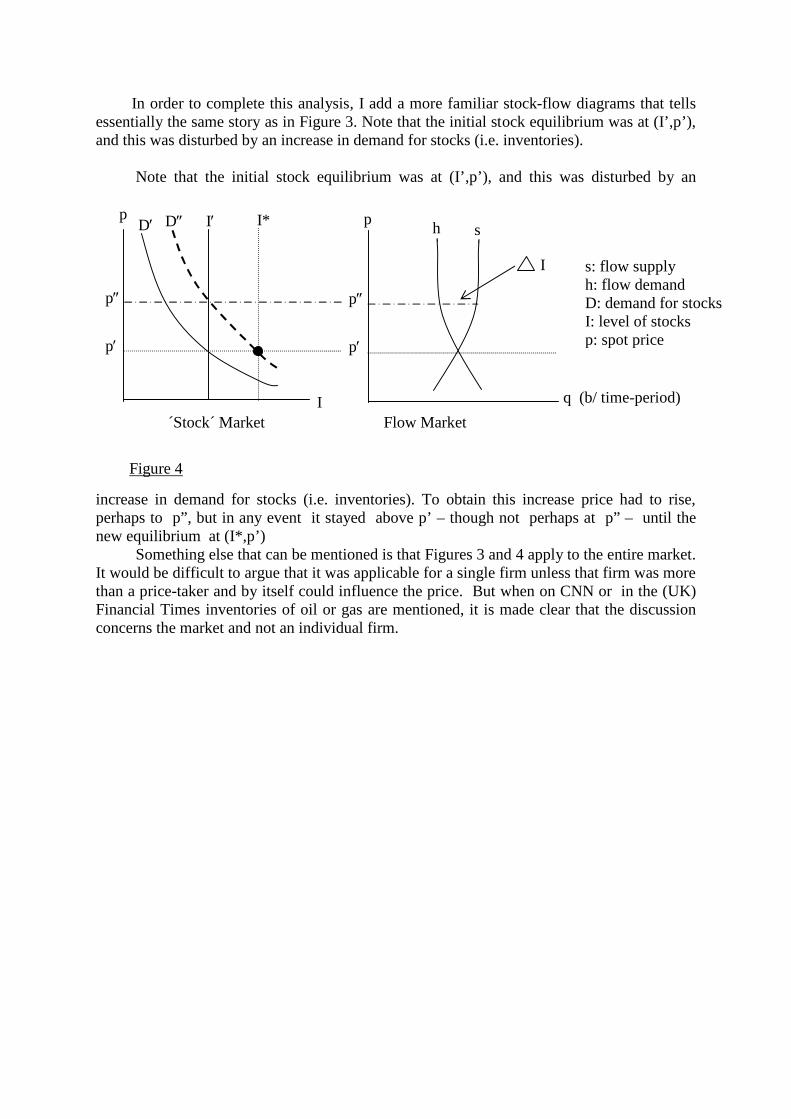
In order to complete this analysis, I add a more familiar stock-flow diagrams that tells essentially the same story as in Figure 3. Note that the initial stock equilibrium was at (I’,p’), and this was disturbed by an increase in demand for stocks (i.e. inventories).

Note that the initial stock equilibrium was at (I’,p’), and this was disturbed by an

increase in demand for stocks (i.e. inventories). To obtain this increase price had to rise, perhaps to p”, but in any event it stayed above p’ – though not perhaps at p” – until the new equilibrium at (I*,p’)

Something else that can be mentioned is that Figures 3 and 4 apply to the entire market. It would be difficult to argue that it was applicable for a single firm unless that firm was more than a price-taker and by itself could influence the price. But when on CNN or in the (UK) Financial Times inventories of oil or gas are mentioned, it is made clear that the discussion concerns the market and not an individual firm.

q (b/ time-period)

s: flow supply h: flow demand D: demand for stocks I: level of stocks p: spot price

s h

p″

p′

p

I

Flow Market I

p″

p′

p D′ D″ I′ I*

´Stock´ Market

Figure 4

7. STORAGE, HUBS AND MARKET CENTERS The natural gas production-consumption process begins with lifting of gas from a ‘field’ or ‘deposit’, and proceeds to a large diameter transmission or ‘merchant’ pipeline, with some gas siphoned off to ‘run’ the compressors, and usually some gas diverted from its ‘end-users’ or ‘final destination’ (i.e. households and small businesses) and into storage, further processing, and sale to very large consumers such as manufacturing industries and electric generators. Eventually it goes into distribution system where pipes are smaller, and via these pipes to homes and smaller commercial establishments, which are customarily designated ‘final consumers’. In Germany, in l995, there were many local distribution companies (LDCs), but since that country has no domestic gas production, the producing (i.e. wholesale) function is largely carried out by Holland, Norway and Russia. The following diagram summarizes this discussion.

Large Industries

Storage is another of those subjects which submits to an interesting theoretical treatment, as you might notice in your book on operations research. On this occasion the exposition will be non-technical, although readers who want to impress others are advised to pay close attention to the terminology. Strangely enough, storage is almost completely ignored in microeconomics textbooks, despite the importance of its presence or absence: when it is absent prices often tend to be extremely volatile, and since domestic supplies of gas are falling, this is one reason why more storage facilities are being constructed in the UK. Gas in storage is turning out to be a carefully watched statistic, particularly in the run-up to winter. Low storage levels mean that any shortages of gas that may appear during the coming months could impact on gas prices, as well as the availability (and price) of other fuels, such

Gas processing

FINAL USERS Households; Commercial establishments

MERCHANT PIPELINE PRODUCING END

Producers

Storage

Power Plants

Figure 4

as heating oil. This is because certain other fuels are substitutes for gas in various uses. The strategy here is to buy gas when it is cheap and store it. A short, easily read and valuable article on this subject is Lee Van Atta (2007), published in one of the best energy forums, EnergyPulse (www.energypulse.net). He mentions that the majority of present storage development in the US has to do with salt caverns, while most of the rest is in depleted reservoirs.

Just as transport involves moving a commodity through space, storage performs a similar function with respect to time – ‘similar’ but not identical, because time runs in only one direction. By putting goods into inventory, we move from the present to the future at finite cost, but returning the exact same goods to the present – and also recreating the background existing when the decision to store was made – is conceptually a much more difficult operation. and for the most part impossible. This suggests that we have a consistency problem: at time ‘t’ we make a plan for t+1, t+2,…, t+x,…,t+N, where N is the terminal date, but it might happen that at e.g. t+x, we perceive that the decision taken at ‘t’ was sub-optimal. A new plan can then be put into practice, but conceivably we would have been happier if we had gotten things right in the first place, or formulated a strategy that would have taken into consideration the possibility of making expensive mistakes. This strategy might have featured storing more or less of the commodity, and relying more heavily on such things as futures and forward markets. Obtaining increased flexibility usually involves a cost.

An important and accessible article on storage is that of Benoit Esnault (2003), although it contains one implication that I have some difficulty accepting. This is that deregulation is a logical precursor to a decrease in prices and improvement in service. Such was the theory when electric deregulation was adopted, but if it is true that the ultimate object of deregulation was lower prices, then I take enormous pleasure in noting that electric deregulation has failed, is failing, or will fail just about everywhere. What we also have here – at least in some countries or localities – is a nice example of the consistency problem mentioned above. By that I mean the absence of a strategy for automatically reversing a sub-optimal venture (e.g. deregulation), and thereby mitigating the bad news that might unexpectedly appear.

A concept that is unique for storage is the convenience yield. This is explained in some detail in my first textbook (2000), but roughly it is the yield (i.e. gain) associated with greater flexibility that might devolve on the owners of inventories. For example, the availability of inventories permits output to be increased without incurring the expenses that are often unavoidable when it is necessary to resort to spot purchases in order to fulfil contract stipulations, or for that matter purchase futures or options contracts at prices that are regarded as unfavourable. The theory here is straightforward: an additional unit put into inventory can provide a sizable marginal convenience yield if inventories are small, while with very large inventories, the marginal convenience yield (associated with adding another unit) might be zero (although the convenience yield would still be positive and could be very large). In the simplest of cases inventory accumulation would continue until the cost of a marginal unit outweighed its marginal convenience yield, with both cost and yield measured in some convenient monetary unit. Another way of viewing this is to say that having access to storage encourages the transfer of consumption from periods in which its value is low to those periods when it is higher (e.g. peak periods).

In examining this issue, it can be argued that gas storage can not only moderate upward price movement, but also function as an excellent hedge against price and volume uncertainty. With natural gas – as with electricity – one of the key issues is peak demand. If a storage option is available, the exposition above indicates that gas is stored during off-peak periods and, if peak demand (or a ‘glitch’ of some sort in transmission or distribution) jeopardizes the ability to deliver desired quantities to end users, then gas is removed from storage. (Electricity cannot be stored, and so this procedure cannot be employed, but peak demand is satisfied by holding some equipment idle during off-peak hours.) An expression

that might appear here is ‘peak shaving’, which sometimes brings a frown to the faces of energy economics students, but it means no more than releasing gas from storage into a pipeline during periods of maximum demand (i.e. peak periods). Possessing this option might make investment in additional producing or transmission capacity unnecessary.

Quality can also be brought into the storage picture. Depleted reservoirs are often used, but withdrawal is relatively slow from these structures. Salt caverns are better and allow rapid injections and withdrawal, which as Van Atta (2007) points out makes them attractive for traders who want to “capture value from price volatility”. What this means is that when they have an opportunity to make some serious money, they do not want to be hindered by an inability to obtain the commodity that they are holding in storage and can be sold at premium prices.

Hubs are physical transfer points that are sometimes called ‘pipeline interchanges’. They make it possible to redirect gas from one pipeline into another. However, at the present time, I prefer not to accept a recent report which claimed that spot prices at Henry Hub, which is one of the largest and best know gas market hubs in the world (and is close to the Lake Charles (Louisiana) LNG terminal) have assumed the role of international reference prices. This kind of claim is sometimes tied to the belief that a large expansion in the trade of liquefied natural gas (LNG) will eventually lead to an international market that is capable of replacing regional markets of one type or another. In the very long run, this hypothetical international gas market would comprise – via uniform net prices – both pipeline gas and LNG.

Even a survey of this length is not the place to speculate on a scheme of this nature, although if the demand for gas in the US reaches the levels predicted by the US Department of Energy, then it will mean that the movement of LNG toward the US will increase to a point where there will be upward pressures on gas prices in every market. Moreover, this is only the beginning. According to one prediction, China and India are expected to double their use of coal by 2030, and their combined oil imports are expected to surge from 5.4mb/d in 2006 to at least l9.1mb/d in 2030. To offset the environmental deterioration that this is liable to bring about, they will almost certainly be in the market for huge amounts of natural gas, and perhaps before reaching these estimated upper reaches, because in my opinion the oil production for 2030 that has been predicted by the IEA and the USDOE for 2030 cannot possibly be realized.

In theory it might be desirable to combine hubs with market centers, where either of these might provide facilities that permit the buying and selling of services such as storage, brokering, insurance and wheeling – where wheeling means the provision of pure transportation services between external transactors. For pedagogical reasons, hubs are often portrayed as displaying a radial system of spokes (i.e. pipelines) and conceivably these spokes could be joined by adding short links.

Market centers are supposed to be able to operate independently of facilities for producing, transporting or storing the physical product, but even so, it might be optimal if they provide a locale where shippers, traders, etc, can buy and sell transportation, gas, etc. To a certain extent the layout of these establishments could take on the structure of trading facilities in the financial markets. If there are imbalances anywhere, then in an ‘ideal’ market center there will be a mechanism where they can be located in a very short time and rectified, which might include providing access to tradable pipeline space and also storage capacity. In the US for example, market centers have direct access to almost 50% of working gas storage capacity and, in general, enjoy a special relationship with many of the high profile storage establishments. (Working gas is the amount of gas in a storage facility in excess of the ‘cushion’ or ‘base’ gas that is needed to maintain facility pressure and deliverability rates.) Regardless of the actual configuration, it is hard to avoid the conclusion that market centers will tend to form at, or in the vicinity of hubs, and that the number of arbitrage paths that can

be utilized for obtaining uniform prices in a system are expanded if there is a proliferation of hubs, market centers and storage facilities.

8. PRELUDE TO A BLUNDER, AND A NOTE ON ‘MERIT ORDER’ Since the publication of my gas book (1987), great changes have taken place in this market. The growth in the demand for gas exceeds that of all energy media except renewables, and unlike the situation 15 years ago, gas comes highly recommended as an input for power generation. (In the UK, more than 70% of power is generated by gas or coal-fired power stations.) A main reason is the advent of combined cycle gas burning equipment with a very high efficiency. What happens here is that in addition to the gas turbine, there is a secondary turbine producing steam from the waste gases/heat of the main gas turbine. The kinetic energy in this steam is transformed to mechanical energy that turns a generator. This generator produces additional electricity for a given input of gas. However, as often happens, there are very many misconceptions in circulation about natural gas, the most pernicious of which – at least in Europe – have to do with its restructuring (i.e. deregulation/liberalization) of gas markets. Some question needs to be asked as to why and how these misconceptions came into existence, and it appears that the answer has to do with the very short time horizons of some producers, as well as the short time horizons and carelessness of consumers. In some parts of the world producers have expressed and conducted themselves in such a way as to suggest that there is virtually an infinite amount of natural gas reserves available for exploitation, although in many regions demand can only be satisfied by very large imports from distant sources. For instance, in much of the North America, exploration/production have been yielding disappointing results for a long time, and expectations about e.g. the Gulf of Mexico and imports by pipeline from Canada often have an air of unreality about them. Similarly, the UK was once a major gas power, but now imports about 40% of its requirements. Many countries, like e.g. the UK and Turkey, are locked into gas due to past investment which emphasized acquiring gas-based generators.

With certain exceptions, many gas buyers are almost totally unaware of how supply and demand could develop in even the present decade, and instead continue to make plans for a future in which they believe that they will have access to all the gas that they will need, at prices that resemble those of the recent past. This might be a good place to note that in Brazil, starry eyed deregulators counted on gas based electric power being cheaper than hydroelectricity. As they now admit, this incredibly gauche supposition was completely wrong. According to the International Energy Agency (IEA) of the OECD, fossil fuels will account for 90% of the world primary energy mix by 2020, which is a big increase over 1997. Global gas demand is expected to rise by 2.5-2.7%/y, with the big consuming area being Asia, where it has been suggested that demand will increase by an average of 3.5%/y between 2001 and 2025. The share of gas in world energy demand could move in that period from 21% to at least 24%. (Oil’s share should fall, but this will be more than compensated for by the increase in world oil demand.) Another estimate has the average global gas production increasing by 2.75%/y to at least 2025, and gas passing coal as the second most important energy medium. Of course, the IEA could be mistaken. Their forecast for oil in 2030 is 120mb/d, which is a very different figure from the one circulating in the executive suites of the major oil producers. World gas prices should eventually display an unambiguous upward trend. In picturing US prices remaining flat until 2005, the IEA was clearly mistaken, but they are correct in noting that a tightening of US and Canadian gas supplies is probably unavoidable, and this process could turn out to be very unpleasant. A wellhead price of $2.5/mBtu (in 1997 prices) for purely conventional US gas in 2020 did not seem particularly realistic to me when it was

predicted, and the upward trend recently experienced in gas prices may be cancelling out the favourable economics of gas-based power generation that resulted from advances in combined-cycle technology.

That brings us to the impact of liberalisation/restructuring. Here the IEA has mostly got it completely wrong on liberalisation in the electricity sector, and as a result I see no reason to expect an improvement in their ability to analyse the economics of world gas. However, since even the experts of the IEA are capable of comprehending that major uncertainties exist about the ability to develop and transport the more distant gas reserves, then it might be in order to suggest that considerable effort should be made to prevent the cavalcade of unsound ideas about deregulation/liberalisation from getting in the way of sound engineering practices. I think it useful to stress that the same exaggerated claims that were made for electric deregulation have also been made for gas, though not so aggressively as a decade ago. To this it can be added that where gas reform is concerned, the economics debate is not particularly encouraging, and in some cases is conducted by academic economists without the slightest feel for either the economics or the engineering aspects of the natural gas sector, and this includes economists with a modicum of engineering training in their background. They have not bothered to find out, for example, that an important component of the financial sector – in the form of several leading investment banks that are heavily involved with commodities – have scaled down their risk management commitments in some commodity markets. Warburg Dillon Read – the investment banking arm of UBS – closed down its energy and electricity derivatives business as early as 1999, and in the same year Merrill Lynch announced its withdrawal from over-the-counter derivatives in natural gas. While this was going on, a consensus of commodity traders and analysts were still willing to wager that derivatives activity in gas and electricity would take off once market liberalisation achieved a critical mass, and as it turned out, in electricity that condition was not too long in coming, although it did not turn out to be durable: it barely lasted long enough for the most important commodities exchange in the world (NYMEX) to declare its electricity futures contract hopeless, and also to cancel one of its natural gas contracts. (Let me note however that these contracts may already have been resuscitated. Wherever there are people who are sufficiently naïve to buy suspicious assets, those assets are certain to appear.)

Now for some particulars. Natural gas deregulation began in the U.S. about 20 years ago, and while I lose no opportunity to declare that I am an opponent of almost all electricity and natural gas deregulation, I remain sympathetic to the natural gas buyers and others in the US who felt that the regulatory climate at the time of the ‘gas bubble’ in that country did not correctly address either efficiency or equity concerns. What eventually happened though was that economists, consultants, and various ‘researchers’ were provided with a forum in which they could unleash a barrage of unscientific ideas for correcting what they construed as existing shortcomings, while at the same time promoting a radical transformation of the entire natural-gas sector – from ‘wellhead’ to ‘burner tip’. The first (non-technical) chapter of my new energy economics textbook attempts to convey some of the total lack of realism by deregulation enthusiasts. How should we treat a collection of misjudgements of the magnitude and extent involved here. In my textbook, I did not treat them at all, because unlike the electric deregulation travesty, gas deregulation was never able to get up full steam. One of the reasons for this was that in the US, and perhaps elsewhere, some important politicians and industry people, as well as genuine experts from the academic world took issue with gas deregulation proposals. For instance, they pointed out that the natural gas market in the US is not informationally efficient. This means that gas prices at widely separate localities do not follow each other in a manner which makes it possible to conclude that – when transportation costs are taken into consideration – these places are in one market, and thus the kind of arbitrage can take place which allows consumers faced with high prices to gain by

buying in markets with lower prices. And not just in the US. A former CEO of British Gas went so far as to contend that the “half-baked fracturing” of the gas markets in order to bring about competition is essentially counter-productive, and a similar argument is apparent in the work of Philip Wright .

Someone else with an important observation on this topic is Professor David Teece of the University of California (1990). According to him, market liberalization in the US has already “jeopardized long-term supply security and created certain inefficiencies.” He also notes that “While more flexible, a series of end-to-end, short-term contracts are not a substitute for vertical integration, since the incentives of the parties are different and contract terms can be renegotiated at the time of contract renewable. There is no guarantee that contracting parties will be dealing with each other over the long term, and specialized irreversible investments can be efficiently and competitively utilized.”

I advise my students to avoid worrying about guarantees where this topic is concerned, given the bizarre intentions of the Energy Directorate of the EU. For instance, assuming a ‘path’ (in e.g. the form of a pipeline) between two markets, and the cost of shipping gas is �ρ� per unit, then prices (p) in these markets should lie within a distance �ρ� of each other, or d(p1. p2) ≤ �ρ�. If there are not paths, however, then at one time – and perhaps even today – the energy experts in the EU Energy Directorate expected billions of dollars to be invested in creating them, although the thinking here reduces to ideology and not economics or engineering.. This is why a colleague of mine in Milan once used the expression “Stalinist” to describe deregulation. Although the various misunderstandings about derivatives markets (e.g. futures and options) have always been fascinating to me as a teacher of economics and finance, they are paltry in comparison to uncertainties created by the transition from what some observers call ‘planning’ to what they interpret as the freedom of spot markets.

As far as I am concerned, large and complex gas systems operating in a climate of uncertainty are most efficiently run on an integrated basis that emphasises long-term contracting. This kind of arrangement promotes optimally dimensioned installations, and although this may not be mentioned in your economics textbook, if pipeline-compressor-processing systems which fully exploit increasing returns to scale in order to obtain minimum costs are to be readily financed and expediently constructed, then – as I interpret the evidence – the kind of uncertainties associated with short to medium term arrangements should be kept to a minimum. Failing to do so could cause a reduction in physical investment, and in the long run lead to higher rather than lower prices. It was the proposed shift from bilateral transactions to spot markets that contributed to what is sometimes called deregulatory uncertainty, and a possible shortage in local (generator) capacity in the California and Alberta electricity markets. This, together with the move to deregulated oligopolies, was a principle determinant of the ruinous electric price rises faced by many households and firms in California, and perhaps elsewhere. In Europe, the EU Commission initially mandated gas market restructuring by 2005. While I can imagine that they were sincere when they concocted this absurdity, I would be very surprised if they sincerely believe any longer that restructuring can or will be taken much further than liberalization, by which they mean that anyone, anywhere, should be able to buy anything that they can afford, and if this ‘anything’ is not for sale, then the rules should be changed so that it could eventually be put on the block. The rest of the restructuring/deregulation package – bringing into existence what they originally announced would be the kind of ‘gas-to-gas’ competition that is supposed to provide consumers with huge savings – will have to wait, and probably indefinitely.

One of the reasons for this is almost certainly a morale problem among deregulation proponents due to the widespread failure of electricity deregulation, but another is the negative attitudes displayed by a number of high profile industrialists and important economists. An example of the latter is Mr Ron Hopper, who was with the US government’s Federal Energy Regulatory Commission (FERC) for 11 years, and as a private consultant was

an advisor to the EU Energy Commissioner, and also the ‘regulator’ OFGAS (in the UK). Hopper calls himself a strong believer in deregulation, but even so he said that “It is difficult for me to see the potential for pipeline-to-pipeline competition” (1994).

Although I lack Hopper’s insight in this subject, it is not “difficult” for me: it is impossible. I also have a problem comprehending why local distribution companies and consumers in the US have been unable to understand that they might be forced to pay billions of dollars in transition costs in order to go from regulation to reregulation. Note: not in going from regulation to deregulation, but in going to a difference brand of regulation, at least for the foreseeable future!

To a certain extent, these payments were exactly what happened. Consumers and distribution companies (i.e. utilities) were burdened with higher costs, and found themselves assuming additional increments of the price risk that accompanied the various changes that were initiated. One of the reasons why things did – and were intended to – turn out this way is because, according to the deregulators and their academic booster club, consumers and distributors were going to be big winners once changes were installed, although this windfall might appear later rather than sooner. (This is also the kind of curious reasoning that the European Union movers and shakers specialize in.) As for the matter of reliability, this was simply overlooked or ignored, although as the leading business publication Forbes (Jan 22, 2001) intimated, deregulation has “whittled away” the guarantee that many gas users in California had of a secure gas supply, since e.g. pipeline companies no longer had the incentive to resort to as much expensive underground gas storage as before, nor to employ long-term contracts (with producers) to the same extent. Let me summarize the discussion above by saying that the talk about gas-on-gas or pipeline-to-pipeline competition in the face of monopoly in Russia and perhaps elsewhere is sheer crank, at best.

To my way of thinking, the discussion above should be more than sufficient to convince alert readers and others that the corporations that have provided European consumers with plentiful supplies of low-cost natural gas for the last 3 or 4 decades should be allowed to carry on their business in the traditional manner. According to Tungland (1995), eccentric attempts to manipulate the laws of mainstream economics might prevent the mobilization of sufficient capital to realize economies of scale, and to shoulder the cost of projects with very long lead times. This was his response to Professor Peter Odell, who had somehow come to believe that such things as regulation and fragmentation could compensate for rising production costs and, apparently, a decline in the physical availability of gas and oil.

I am now going to take a brief look at merit order, and by way of moving into this topic, a comment seems appropriate concerning the use of gas to generate electricity in a deregulated setting. Electricity deregulation has failed just about everywhere, because in countries where there is no excess generating capacity, prices tend to rise as demand rises, and since managers prefer more money than less, they do not bother to make the investments in additional capacity that deregulation enthusiasts said they would make, and which consumers thought would be the case.

But it is more complicated than that, because there are situations in which investments are made, but even so prices increased. A good example here is where investments are made in gas-based capacity instead of e.g. nuclear or coal. The advantage with gas is that in the short run it is more profitable, since as explained at great length in my energy economics textbook, capital costs are lower for gas based generating equipment; however as was not explained in detail, gas prices have a tendency to be very volatile – and in addition have been on an upward trend over the past five or six years. As a result, consumers inevitably find themselves presented with much higher gas bills. Moreover, even if the daydreams of the deregulation booster club are realized, and generators (logically) construct smaller facilities, and there are many of them – thus giving the appearance of a competitive market – it does not make a great deal of difference to consumers because all generators might be exposed to high and volatile gas prices, which they do not hesitate to pass to their customers.

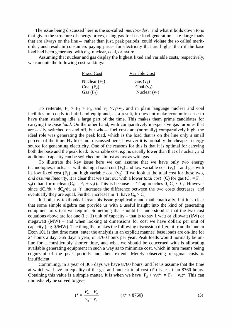
The issue being discussed here is the so-called merit-order, and what it boils down to is that given the structure of energy prices, using gas for base-load generation – i.e. large loads that are always on the line – rather than just. peak periods could violate the so called merit-order, and result in consumers paying prices for electricity that are higher than if the base load had been generated with e.g. nuclear, coal, or hydro.

Assuming that nuclear and gas display the highest fixed and variable costs, respectively, we can note the following cost rankings:

Fixed Cost Variable Cost

Nuclear (F1) Gas (v3) Coal (F2) Coal (v2) Gas (F3) Nuclear (v1)

To reiterate, F1 > F2 > F3, and v3 >v2>v1, and in plain language nuclear and coal facilities are costly to build and equip and, as a result, it does not make economic sense to have them standing idle a large part of the time. This makes them prime candidates for carrying the base load. On the other hand, with comparatively inexpensive gas turbines that are easily switched on and off, but whose fuel costs are (normally) comparatively high, the ideal role was generating the peak load, which is the load that is on the line only a small percent of the time. Hydro is not discussed here, however it is probably the cheapest energy source for generating electricity. One of the reasons for this is that it is optimal for carrying both the base and the peak load: its variable cost e.g. is usually lower than that of nuclear, and additional capacity can be switched on almost as fast as with gas.

To illustrate the key issue here we can assume that we have only two energy technologies, nuclear – with its high fixed cost (Fn) and low variable cost (vn) – and gas with its low fixed cost (Fg) and high variable cost (vg). If we look at the total cost for these two, and assume linearity, it is clear that we start out with a lower total cost (C) for gas (Cg = Fg + vgt) than for nuclear (Cn = Fn + vnt). This is because as ‘t’ approaches 0, Cg < Cf. However since dCn/dt < dCg/dt, as ‘t’ increases the difference between the two costs decreases, and eventually they are equal. Further increases in ‘t’ have Cg > Cn.

In both my textbooks I treat this issue graphically and mathematically, but it is clear that some simple algebra can provide us with a useful insight into the kind of generating equipment mix that we require. Something that should be understood is that the two cost equations above are for one (i.e. 1) unit of capacity – that is to say 1 watt or kilowatt (kW) or megawatt (MW) – and when looking at dimensions for cost we have dollars per unit of capacity (e.g. $/MW). The thing that makes the following discussion different from the one in Econ 101 is that time must enter the analysis in an explicit manner: base loads are on-line for 24 hours a day, 365 days a year, or 8760 hours per year. Peak loads would normally be on-line for a considerably shorter time, and what we should be concerned with is allocating available generating equipment in such a way as to minimize cost, which in turn means being cognizant of the peak periods and their extent. Merely observing marginal costs is insufficient.

Continuing, in a year of 365 days we have 8760 hours, and let us assume that the time at which we have an equality of the gas and nuclear total cost (t*) is less than 8760 hours. Obtaining this value is a simple matter. It is when we have Fg + vgt* = Fn + vnt*. This can immediately be solved to give:

t* = ng

gn

vvFF

−

− ( t* ≤ 8760) (5)

Now for a key recognition. When t < t*, and one unit of capacity is to be added, it should be gas; while if t > t*, and one unit of capacity is to be added, it should be nuclear. This can be easily proved. Let us examine the cost situations at t* θ, where θ >0. Then we have Cn = Fn + (t* - θ)vn and Cg = Fg + (t* - θ)vg. The next step is to compare these two linear cost equations:

Cn – Cg = (Fn Fg) + (t* θ) [vn vg] = (Fn Fg) + (t* θ)

−

*tFF gn

In this expression the value of vn – vg was obtain from (5). This can be simplified to give:

Cn – Cg = (Fn – Fg)

−

+*

*1t

t θ (6)

The right hand side of (5) is unambiguously positive, and thus Cn > Cg when t < t*. A similar manipulation will show that when t > t* we have Cn < Cg. As shown in my textbooks, the reasoning in this example is valid even if we have more than two types of equipment. What is not shown in my textbook is a mainstream profit maximization exercise, however this is sketched in the appendix to this paper.

9. RUSSIAN GAS, AND SOME COMMENTS ON LNG

The production of energy is the moving force of world economic progress. -Former President Vladimir Putin

Almost a year ago Professor Jonathan Stern of Oxford University visited the Stockholm School of Economics, where he presented a ‘pop’ version of Russian gas intentions in both their own country and regions west of the Russian border. So many dubious statements were launched by Stern and local ‘researchers’ during that low-level get-together, that I found myself painfully aware once more of the macroeconomic and political catastrophe that may someday arrive because of a sudden shortage of energy resources – a condition that at least partially has its basis in the grotesque failures to teach and/or promote realistic versions of energy economics.

In the wake of the ‘Georgia Incident’ that began around the opening of the 2008 Olympics, it appears that there has been a large-scale pilgrimage back to cloud-cuckoo land – both to reveal and scrutinize Russian geopolitical intentions, and to a lesser extent to circulate some bizarre opinions about the availability or non-availability of Russian energy resources. Recently a short article appeared in Newsweek claiming that oil and gas passing through Georgia was supposed to “free Europe from Russia” but, according to its author, “NOT ANYMORE”. How anyone could believe that the prevailing gas superpower, Russia, was capable of having its ambitions thwarted by a few pipelines from the interior of central Asia, is something that deserves the attention of psychologists or psychiatrists and not readers of a weekly news publication.

There were probably many items in my gas book (1987) that prevented it from becoming the favourite bed-time reading of various gas experts, but almost certainly one of them was my contention that there should be more cooperation between the producers and consumers of energy resources, to include Russia and OPEC, because my position then – as now – is that there is an unavoidable shortage of gas (and oil) on the horizon, and it is

important to use what is left of these resources to smooth out the transition a new global energy economy – probably one emphasizing nuclear and renewables. A gentleman who apparently had some difficulty with this concept was former U.S. president Ronald Reagan, as well as his advisors, because instead of buying gas from the Soviet Union, these energy gurus thought that some effort should be made by European consumers to obtain the supplies they required from e.g. Africa and Argentina, arguing that by doing so it would weaken the Soviet economy.

Obviously, the chief executive was constitutionally and intellectually unable to accept a sensible strategy, which was to contract for the largest possible quantities that could be obtained from the Soviet Union, and to encourage that country to invest in (and fill) the largest possible pipelines. The basic issue was not merely safeguarding and expanding Western Europe’s supplies of gas in the years to come, but increasing the general accessibility of all energy materials, to include those purchased by the United States (and its friends and allies) from any supplier. (It was also possible, or even likely, that another of President Reagan’s theories was that a return of the Taliban to Afghanistan was desirable and should be expedited. If so, I would like to go on record as saying that the war now taking place in that part of the world could be in full swing when music begins at the New Year’e eve parties celebrating the arrival of the 22nd Century.)

When I pointed out the advantages of doing business with Russia in a talk at Cambridge University, and in addition suggested toning down Cold War rhetoric, a number of observers – to include the founder of the influential publication Geopolitics of Energy, Melvin A. Conant – assured me and everyone else within earshot that although the ideological commitment of the Soviet Politburo was ostensibly to Marx and Lenin, it held a high regard for dollars and deutschmarks, which made Soviet gas industry executives prone to discharge their business obligations. In the Newsweek article referred to above, it was stated that European gas buyers have excellent relations with Russia and do not fear greater dependence. In addition Germany is supposed to be building its own pipeline through the Baltic Sea to guarantee its supply of Russian gas.

I know enough about this pipeline to believe that the persons in this country (Sweden) who study this project should learn to ignore the precious wisdom dispensed by Oxford University pundits and certain journalists. There has been some delay with this conduit that is at partially due to strange ideas in Sweden as to the ulterior purposes of the Russians, when the most likely agenda of those good people turns on collecting as much money as possible, and sooner rather than later. What needs to be understood is the relationship between the amount of Russian gas coming into Western Europe, and the price of e.g. electricity in most of Europe – a price boosted by the absurd electric deregulation desired by the European Union, in addition to the decision to promote the sale of electricity on the electricity exchange NORDPOOL, which is a sophisticated version of what George Orwell termed an indoor welfare scheme.

According to Jeffrey Michel, this underwater pipeline would allow Russian vessels to avoid a complicated sea passage, and in addition would mean that possible disputes between Russia and Baltic states will not lead to a reduction in gas contracted for Germany and perhaps other countries, or even another Cold-War burlesque. A further observation has been made by the important petroleum consultant Herman Franssen, who notes that Russia is not only an energy powerhouse, but also possesses an enormous amount of unused and underused agricultural land. The efficient exploitation of this land with the possible help of experts from North America and Europe might be essential for feeding hundreds of millions or even billions of persons outside Russia..

Several years ago the kingpins of the European Union (EU) held a meeting at which the availability of Russian natural gas and oil was discussed at length, and the Financial Times (March 23, 2006) suggested that the sale of Russian gas to China and Japan might have a negative effect on the energy prospects of Europe, which relies on Russia for at least 40% of

its gas. By extension, in the long run, this could have a negative effect on North America, because the global gas scene has started to take on some of the features of a mainstream textbook market, due (among other things) to the ability of huge liquefied natural gas tankers to deliver ‘spot’ cargoes. The new carriers, known as the QFlex and MFlex are designed to take 210,000 tonnes and 260,000 tonnes of LNG respectively, compared with the traditional sized tanker loads of 135,000 tonnes and 145,000 tonnes.

In referring to a “textbook market” I mean a market with more flexibility than a conventional LNG market. For instance, instead of a portfolio of long-term contracts in which gas carriers are locked into predetermined routes, British Gas (BG) now tries to structure its operations so that gas can be diverted to buyers that are willing to pay premium prices. At the same time it should be appreciated that the majority of LNG business must involve long-term (and relatively inflexible) contracts because otherwise financing would be more costly. Financial institutions are generally unwilling to enter into the kind of arrangements favoured by men like Aristotle Onassis and competitors.

For readers who, like myself, prefer to deal in cubic feet, 1 tonne of LNG is roughly 48,000 cubic feet of natural gas, and the liquefaction process that changes gas to a liquid involves a volumetric transformation of 1/600. Today there are about 150 LNG tankers, and Simmons International has calculated that a new project costs on average 1 billion dollars for every million tonnes of LNG, .

According to the Newsweek article, a recent Rice University Energy Program modelling exercise found that Russian efforts to deprive Germany of gas would likely be futile, as market deregulation would allow other suppliers to fill the gap. What this half-baked conclusion by the Rice University know-nothings missed is that there are no other suppliers in the short-run, nor perhaps inexpensive suppliers in the long-run. On the other hand, in the short-run Russians could rush to completion any pipelines that they are constructing in the direction of China, and possibly beyond, in which case Germany, perhaps other European countries, and also the United States would find themselves bidding for progressively larger increments of gas.

The running mate of presidential candidate John McCain, Ms Palin, is apparently very positive to larger investments in Alaskan (and perhaps Canadian) natural gas, which would eventually find its way to the US Midwest. This scheme was being discussed in some detail well before my gas book was published twenty years ago, and the cost was generally considered excessive at that time. At the present time the estimated cost may be as much as 40 billion dollars, as compared to the 10 billion that several Russian pipelines toward Asia will ostensibly cost. In these circumstances the ignorant bluster originating with persons like Ms Merkel and Ms Rice should be restrained, because where energy resources are concerned, Russia’s position with regard to alternative markets is so enviable that its government does not have to be impressed with voodoo economics or voodoo politics. If there are very large amounts of exploitable gas in Alaska, Ms Palin’s pet project may make economic sense, but at the same time more attention needs to be paid to ascertaining the amount of gas that may eventually become obtainable from shale deposits in or near the US. These gas sources might eventually be able to greatly help close the large and increasing gap in that country between gas production and consumption which might have reached 15-16 percent. Coal bed methane gas may also have a great deal to offer in the future.

One of the editors of the Financial Times, Martin Wolf, might be described as a cut-rate version of the two ladies mentioned above. He has suggested that Russian “elites” should be punished because Russia overreacted in the Georgian incident. When I was informed of this silly proposition, the only kind of punishment that I could have imagined for those ladies and gentlemen was to prohibit them for a season or two from enjoying the skiing in places like Courchevel and St Moritz. Of course, the French and Swiss governments would have to agree to this foolishness, which I am glad to say is unlikely to happen, regardless of e.g. the bizarre posturing of Monsieur Sarcozy.

Something else that we do not hear much about is a possible participation of the Russians in the growing liquefied natural gas (LNG) market, although that option has been raised by some observers. There has also been some talk about Russian gas exports from the new Sakhalin LNG scheme gaining access to Asia-Pacific markets, which could include utilizing any terminals that might open in India, and also taking advantage of the fact that Indonesia’s gas fields are ageing, and consequently are less attractive to potential customers. It is also interesting to note that the Russians have decided to develop the giant gas field Shtokman without foreign help, and possibly switch it from a source of LNG for the US to a pipeline venture whose gas is destined for Europe.

In theory there should be a place for Russian LNG just about everywhere, because while LNG accounts for only about 2% of the gas used by the US at the present time, the United States Department of Energy (USDOE) has suggested that it could amount to 30% by 2025, with the total demand for gas in the US amounting to about 30 trillion cubic feet. As Mark G. Papa, an important American energy executive once said, “Right now, on the supply side, LNG is the only lever we have to pull” – although this may not be complexly true at the present time. One of the interesting aspects of LNG right now (15 September) is the difference in price between conventional natural gas in the US, and LNG delivered to Asian locations: the first costs almost $8/mBtu and the latter almost $20/mBtu. At bottom this price gap is due to is an increasingly higher linkage between LNG prices and oil prices, due to the increased demand for and shortage of gas in Asia.

In addition, many Americans to not want LNG plants in or near where they live. After an accident in Algeria some years ago reminded environmentalists that LNG (because of its density) has a very large explosive potential, they informed the general public that LNG might prove to be an attractive target for terrorists. California is a state where the opposition to new terminals is very strong and growing, and as a result the next terminal serving consumers in that state will likely be in (Baja) Mexico, just across the border from the key California market. It has been suggested though that the optimal position for new US terminals is the Gulf of Mexico, where they could tap into existing pipeline networks. For an elementary discussion of this and other natural gas issues, the reader is referred to Julie Urban (2006).

At this stage of the discussion it seems proper to remind readers of the process involved in the obtaining by households, small commercial establishments, power generators and heavy industries of conventional gas that at one point was LNG.

The first step is production of natural gas in the manner described in several places above. Next liquefaction, where the gas is chilled and compressed in a manner so that 600ft3 of gas becomes one cubic foot of liquid. After that this liquid is shipped in special vessels, and when it reaches the country in which it is to be used it is regasified. It can then be put into conventional gas pipelines and moved to buyers. It also happens that in the last decade or two costs have been greatly reduced by economies of scale and technological advances, especially in liquefaction. As with pipelines and compressors, the larger the units the greater the cost efficiencies – up to a certain point.

LNG plants have been constructed in the fairly recent past in Nigeria, Australia, Qatar, and Trinidad, and eventually Iran should become a major supplier. In the last five years LNG has grown by almost fifty percent, but apparently demand is still greater than supply. Rumour has it that foreign firms do not want to invest in Iran because it may someday be visited by US bombers, but if bombs begin to fall on that country the price of oil could move off the Richter scale. Besides, with the oil price at its present level, and with the technical ability possessed by Iranian citizens, foreign investment is an option that is far from essential. Algeria was the first country to ship LNG (to the UK, in l964), while Qatar seems to be in the process of displacing Indonesia as the world’s largest LNG exporter.

According to the Financial Times (October 20, 2006), Qatar exports LNG to the US on short term contracts. Why short-term? The answer of course is that they expect the price of

gas to increase, and in addition they and their colleagues in the Gulf are in a position to make a reality of this expectation. The IEA has predicted that before the next decade is over, LNG will account for up to 16 percent of the global demand for natural gas, and there has been some talk recently of the possibility of a gas producers’ organization along the lines of OPEC. Someone who disagrees with this is David Victor of Stanford University, but I have decided to discount Mr Victor’s argument on this subject, and say that there is a finite probability that we could see a producer’s organization for gas some day. I doubt though whether that probability has reached 50%.

The Financial Times has also stated that Qatar intends for its natural resources to benefit that country for the next 100 years. 100 is a nice round number, but if Qatar is serious and the other Gulf countries join them in this agenda, then it is a certain that the period of low energy prices is over for a very long time – until nuclear and certain renewables play a much greater part in the scheme of things than they do now. The government of Qatar has also indicated that it hopes to account for 20 percent of the world’s global gas market by 2010, but this is uncertain. Moving ahead a few years, the IEA estimates that global LNG capacity will reach 600 billion cubic meters by 2015, when LNG is suppose to account for up to 16 percent of global gas demand.

In my written work and lectures on natural gas, I have expressed some surprise at two phenomena. The first is the continued ‘flaring’ of large amounts of natural gas, initially in the Middle East, but now in Nigeria and apparently also in Russia. The problem seems to be a lack of investment in gas-gathering networks, and according to some observers the total amount of gas ‘burned off’ in 2007 had a market value of more than 40 billion dollars. I am also mystified by the failure of Iran to realize its output and export potential, because I can remember talks given by myself and others which predicted that Iranian gas would be of great value to European gas users, and the sooner the better. However, just as the energy in uranium cannot be ignored, the same can be said for the huge gas reserves of Iran. According to the International Energy Agency. Europe’s gas imports will double by 2030, with Russia being the key supplier. This sounds good to me, although it would sound even better if there were more Iranian gas available for Europe. 10. TWO WIDELY DISCUSSED PIPELINE SETS, AND CONCLUSIONS At the present time there are two highly visible discussions taking place about ‘sets’ of pipelines. One of these is the set proposed by Governor Palin of Alaska, and which as far as I know is a ‘singleton’ (or set with only one member), while the other concerns pipelines from the ‘East’ (i.e. Russia) toward what was at one time called West Europe. I believe that this long paper contains almost enough background for readers to understand the arguments of Ms Palin in favour of the pipeline from Alaska, as well as her opponents in the ranks of Big Gas and Big Oil. In addition, readers should be capable of interpreting the position of persons like the American ambassador to Sweden, Mr Michael M. Wood, who on at least one level is operating on the same wave length as a crank ensemble of ‘cold warriors’ who are attempting to sell the notion that the Russian government is up to no good where its energy ambitions are concerned. With all due respect, it is possible – though not certain – that Ms Palin is correct in believing that a pipeline from Alaska is necessary, and its construction should commence in the near future. Moreover, if Mr ambassador could alter his cold-warrior stance, he might find it easier to convince movers-and-shakers that it is a wise move to increase the availability of non-Russian gas to West Europe, if only so that persons like myself will be able to afford longer summer vacations on the marvellous west coast of Sweden.

Some elements of the argument in favour of bringing more gas from e.g. Alaska to the ‘lower 48’ of the US are found in this paper, but serious readers with a taste for algebra should make the acquaintance of a Hollis Chenery paper (1952). I would also like to use this

opportunity to refer to some remarks by Mr Ed Kelley that were reproduced on the important site ‘Seeking Alpha’. Mr Kelley is a vice president of the consulting organization Wood McKenzie, who believes as I do that the (Btu) gas price is due to move closer to the (Btu) price of oil.

The logic is simple. The forecast of the National Petroleum Council (NPC) of the United States is that gas consumption in that country could increase faster than ever. If there is a shortage of domestic gas, then more LNG will become attractive, but price-wise LNG is often in a very different category from domestic gas prices in the US. At the present time ‘spot’ LNG cargos are being sold for 19-$20/mBtu in Asia – which is close to the Btu price of oil – however domestic US gas is selling for $7.8/mBtu. If buyers in the US find it necessary to bid for these Asian cargos, domestic sellers of gas will have an incentive to raise their prices.

On this point, Carol Freedenthal claimed in the Pipeline and Gas Journal (3 September 2008) that American markets have become the “dumping grounds” for excess LNG only when the high priced markets of Asia and Europe are satisfied. Interestingly enough, at one time it was believed that the US would be the most important destination of vessels carrying LNG, but as things turned out a key supplier, Indonesia, lost some of its status in the Asian market due to ageing fields, and as a result cargoes are moving toward the main Asian buyers from as far away as the West Indies.

And could it happen that US buyers will find themselves in the unenviable position of trying to outbid Asian buyers for substantial amounts of LNG? As far as I can tell, before the good news provided the buy side of the US gas market by the unexpected large exploitation of e.g. shale gas, increased spending on exploration and production in the US had only a modest effect on output. The same is true in Canada, which is one of the reasons why the pipeline that is so favoured by Ms Palin would probably feature so-called ‘laterals’ that carry a non-trivial amount of Alaskan gas to Canadian buyers.

In the light of these factors, it easy for me to believe that considerable thought should be given to making it easier for larger amounts of Alaska’s known gas reserves (= 35 Tcf according to Ms Palin) to move toward the ‘lower 48’ as soon as possible, because Asian demand is not going to subside, and it is uncertain if the construction of LNG vessels will keep pace with rising demands. In addition, from 2007 to 2008, global electricity generation rose 4.8% while the nuclear share of electric generation dropped to 14% from a near steady rate of 16-17% between 1986 and 2005. One of the reasons for this decline could well be the intention to use more gas, which seems to be the case in e.g. Sweden.

A problem commonly associated with the ‘Palin pipeline’ is the time that might be required for its construction, although it could be argued that there are circumstances in which there are cost advantages associated with a longer construction periods. In any event, most observers think that it will take at least ten years, and having once studied very carefully the modelling alternatives for the proposed Alaska Highway pipeline, I doubt whether it could be less. Big Gas has judged this pipeline “politically correct but economically dumb”, however personally I am not convinced.

Turning to Europe, Mr Ambassador has specifically objected to any intention to bring more Russian gas into West Europe, either e.g. via a pipeline from Russia that is partially located on the bottom of the Baltic, or for that matter in any other conduit or carrier from Russia. To his way of thinking, that country has become too prominent on the European energy scene. An attitude of this sort sounds to my ears like a Reagan remnant, since former president Ronald Reagan (or his advisors) once came to the goofy conclusion that Europe should regard gas from Africa and Argentina as preferable to Russian resources.

In some sense putting a limit on the amount of Russian gas purchased might not be a bad idea, particularly if more gas could be obtained from Libya and eventually from Iran for the south of Europe. Still, it has to be recognized that according to contemporary estimates, global demand for gas will double by 2025 and European demand will display the same

increase by 2030. In these circumstances I fail to see the wisdom of antagonizing the Russians – especially given the option they possess for replacing sales to Europe by an increase in supplies to Asia. Exactly how easy this would turn out to be is uncertain though, because if a supplier becomes heavily involved with sunk costs (for e.g. pipelines), then – at least in theory – it should make them more reasonable in price negotiations. Of course, several years ago I refereed an article in which the author suggested that the time was approaching when gas sellers should consider forming a cartel. An action such as this would change a great deal, because to my way of thinking international cartels have a great many things in their favour.

Among the objects of this long paper has been my desire to set the record straight about several of the misunderstandings associated with energy economics, to include natural gas. First and foremost I want readers of the literature to understand that when they see references to the work of Harold Hotelling on resources, they should tune out, and if their teacher feels otherwise, then they should think about dropping out. (And, incidentally, Hotelling was a brilliant economic theorist whose work on resources could not possibly have been intended for the nonsensical uses to which it has been put).

Another controversial topic that I spent an hour or two examining when I was lecturing on development economics in Dakar and in Stockholm, and doing research in Australia, had to do with the so-called ‘Dutch Disease’, which concerns itself with the ill health that can plague an economy when it finds itself with a bonanza that has its origin in mineral wealth. Somehow it was originally thought by some confused researchers, before or after the fact, that Holland (i.e. The Netherlands) would be brought to the brink of disaster because of macroeconomic distortions accompanying the exploitation of gas in the super-giant Groningen gas structure. What actually happened was that revenues from gas may have created a very small group of losers, however they meant increased prosperity for almost everyone else. A better example of course is Norway, where enormous revenues from oil and gas have not only secured the well-being of a large proportion of the present generation, but should do the same thing for the next. The exploitation of large mineral resources will always increase aggregate prosperity, assuming an an absence of the kind of gross corruption, stupidity and greed that leads to unnecessary waste.

One of the major themes of this paper is the possible scarcity and rise in price of natural gas, given the rapidly increasing demand for this commodity. In considering this possibility I would like to confess that on many occasions, and in many places, I have delivered aggressive rants about the scarcity of oil, and the movement of oil to a price greater than $100/b seems to have confirmed my predictions. When Armand Hammar of Occidental Oil said that this would be the price at the end of the 20th century, he was judged to have gone off the deep end, but now we have seen that ‘benchmark’ passed, and ‘anomalous’ events are always possible that could make $100/b appear attractive. If Mr Hammar were still with us, it is not unthinkable that he would have similar thoughts about gas.

In attempting to spread a Hammar-like belief about oil and gas, I can remember encounters with persons who were not impressed with my scholarship or harangues, and who informed me that new technologies and knowledge ensure that tolerating and adjusting to high-price oil and gas is always possible, and in the short run. Originally teachers of economics and finance like myself thought that oil at the present price would trigger a macroeconomic disaster, but this has not happened, and so I am just going to mention – en passant – why. The negative effect of this destructive oil price has been lessened by large scale immigration to most of the main oil importing countries, as well as some related changes in income distribution in those countries. As an exercise, concerned readers can elaborate on this statement, and perhaps at the same time attempt to figure out exactly how long this situation will prevail – assuming that they believe that I am correct. Furthermore, the high oil price will pull up the gas price, though possibly later rather than sooner, and if the

financial market was deteriorating while this was taking place, then there would be a danger of a ‘great depression’ replay.

Incidentally, the most peculiar characteristic of the present bad news associated with the international economy has been the large-scale creation of sub-prime financial assets, and their purchase by some of the largest and most important financial institutions in the world, who possess perhaps the most sophisticated research departments. It is not impossible that some of the readers of this article may someday find themselves doing research for those establishments, since they have been so badly served by present analyses.

With electricity deregulation (i.e. restructuring) obviously imploding in many countries or regions, it might be pertinent to mention those aspects of the electricity story that are most relevant for gas. As already noted, first and foremost we should make certain that EVERYBODY understands that restructuring increases uncertainty, and (ceteris paribus) uncertainty decreases physical investment. This is a straightforward neo-classical result, and from the point of view of common sense as well as mainstream economic theory, it is undeniable. At one time in Europe it appeared that deregulation, carelessly mixed with bureaucratic blundering, was a far greater danger with electricity than with gas, given that the EU energy bureaucracy wanted enough investment to take place to avoid a California type situation. But now, with the evidence in, virtually every intelligent observer realizes that it would be best for everybody on the buy side of the market if electric deregulation was passé.

Moreover, in Europe and perhaps elsewhere, restructuring means that a competitive or partially competitive gas purchasing structure could find itself confronted by powerful external suppliers operating in a monopolistic or oligopolistic mode, and Russia is not the only supplier that I have in mind. As widely known, gas buyers in Spain are unhappy with the ambitions of Algerian suppliers. Thus the already high price of gas to that country could go higher, to the detriment of large firms as well as households and small businesses. In the US both former Energy Secretary Spencer Abraham and former Federal Reserve Chairman Alan Greenspan have pictured the present development of natural gas prices as a threat to the US economy on the same plane as an escalation in oil prices. A mitigating factor may have appeared however in the form of a large increase in the production of shale gas (i.e. gas under huge deposits of shale that can be exploit with horizontal drilling), however the jury is still out concerning the exact dimensions of this bonanza.

Put more directly, it might have been a mistake to become so thoroughly attracted to natural gas. A good example here is the situation in e.g. California, where a very large percentage of new capacity is apparently fired with gas. Moreover, faith in the availability of gas appears to have been so extensive that a large percentage of the new gas-based power plants lacked fuel-switching capacity, and it unfortunately seems that the older facilities with a fuel switching option were, on the average, less efficient. Moreover, according to Eric Smith, environmental regulations (about air quality) have helped to eliminate economic arguments for dual capacity. Thus the efficiency and versatility of the entire system is less than it should be had the natural gas booster club been kept in its place, and nuclear received a better hearing.

I find it stimulating to report that the majority of energy professionals are coming to their senses where the above topic is concerned, and as icing on the cake, considerably less tolerance is being shown the ravings of flat-earth economists and their adherents where future supplies of gas and oil are concerned. What is happening is that these ladies and gentlemen have started paying closer attention to reality than to the kind of bizarre economic theory that became popular in the U.S. during the presidency of Ronald Reagan and the heyday of his guru Professor Milton Friedman, who at one time thought that the oil price would descend to $5/b. Despite the recent success of shale gas, from a production point of view the domestic US gas future does not appear promising, and as a result more than a few important firms now regard that region a hopeless case for large scale future investment, even if gas prices

continue to rise. Furthermore, as in the US, increased drilling in Canada is not raising production by a substantial amount. The situation in both countries is probably best summed up as follows: mature basins, smaller discoveries, and a high rate of natural decline from existing gas wells – which unavoidably translates into higher production costs and higher prices.

As alluded to earlier, Mexico is not going to provide much help to US gas consumers. Mexico is slowly being transformed into a large importer of gas. Something worth emphasizing is that even if a substantial Canadian export capacity became available, in order to provide large amounts of gas to the US very expensive pipelines will be necessary. I have also heard it argued that increased drilling in traditional gas producing regions in Canada is not increasing production by the expected amount, and in the Western Canada Sedimentary Basin (WCSB), production from gas wells – on the average – has been declining at almost 6%/year for the last nine years. It may also be true that in Canada, as in the U.S., large producers are more likely to busy themselves with cost reducing mergers rather than devoting scarce time and money to expensive investments in new capacity. The managers of these enterprises learned long ago that large fields take a long time to develop, which is something that is often overlooked by those journalists whose attention is usually concentrated on listed reserves, and at the same time believe that a flow from a stock of reserves can be obtained in no more time than it takes to manipulate supply curves in textbook presentations.

What some observers might have overlooked – deliberately or otherwise – is that the natural gas industry is inherently less flexible than e.g. the electricity industry. Because the electricity sector is subject to Kirchoff’s laws, many students of deregulation think that is easier to control flows in the gas sector, and thus bring about the amount of network price adjustments required to obtain (via arbitrage) the utopian results promised by the deregulators. As mentioned earlier, spot prices at widely separated points in large gas networks are generally not related to each other in such a way that it is possible to claim that they are in one market, and this is largely due to coordination problems that are almost unavoidable due to erratic shifts in the demand for gas. In addition, time lags are unavoidable in scheduling deliveries, which results in a sub-optimal use of storage and transmission capacity that is further distinguished by the frequent appearance of transactional bottlenecks. Deregulation is not likely to improve this situation. Even the electricity market is more accommodating when it comes to avoiding ‘glitches’ of this nature.

In selling electricity and gas deregulation to the voters, among the pseudo-scientific arguments first employed were that increasing returns to scale were a thing of the past. A competent teacher of economics or engineering should be able to expose this myth in a half-hour by employing some secondary-school algebra or ‘soup-bowl’ type cost diagrams to interpret the relationship between the expected growth rates of gas and electricity consumption, and the incentive to take advantage of scale economies (or sub-additivity) of the relevant cost functions. Accordingly, one way in which this matter was approached was to complicate it by claiming that sub-additivity was absent in these industries, and thus introducing into the discussion technical matters that most readers took considerable pains to avoid. As it happens though, the relevant materials on sub-additivity (or increasing returns to scale) are easy to locate in the intermediate economics literature, and equally as easy to comprehend. Another way of approaching this issue is merely to ask managers and engineers in the gas (and electricity) industries whether they believe in the non-existence of increasing returns to scale.

John Stuart Mill, in his Principles of Political Economy (written in l848), remarked that “the laws and conditions of production partake of physical truths. There is nothing arbitrary about them.” Except, to partially quote U.S. Congressman Peter de Fazio, when we are dealing with people “who are going to make millions and billions”. These are persons willing to do and say anything that will convince the consumers and businesses on the buy side of gas and electricity markets that restructuring will enable them to make hundreds and

thousands. This happened in Sweden where deregulation allowed power firms to invest in existing foreign generating capacity rather than new domestic facilities. Regardless of how we approach oil-gas-electricity markets, we inevitably see conduct which suggests that we do not have the perfectly (or even partially) rational transactors mentioned in your favourite economics textbook. In New Zealand, as elsewhere, there are a number of theories about what went or is going wrong with the domestic energy supply. The simple truth is that nothing has gone wrong; globally, oil and gas have become scarcer, and the consequences are that in most countries consumers and producers will just have to learn to transact their business against that unpleasant background instead of the make-believe world of infinite supplies of energy that they were promised by the flat-earth economists. When I first worked in Australia, the giant Maui gas field in New Zealand was considered a priceless asset, and virtually nobody took the trouble to think of it as having a finite ‘lifespan’. Now it is in sharp decline, with apparently only a few years’ of what are sometimes called ‘recoverable’ reserves left., by which it is evidently meant reserves that can continue to supply gas at the production levels of a decade ago.

I can begin closing this long survey by suggesting that an understanding of the political and economic circumstances of that New Zealand gas decline would provide a valuable intellectual experience for anybody believing that even today we are running ‘into’ rather than out of oil and gas. These pseudo-scholars and amateur researchers are making a dismal contribution to the traumatic situation that could occur should global oil and gas production unexpectedly begin to level off.

I also want to note that there are academics and assorted paid and unpaid propagandists who have decided to inform everyone in their ‘network’ that the high oil and gas prices now being experienced are irrelevant from a macroeconomic and financial market point of view: ostensibly, today’s economies have become so sophisticated when it comes to saving energy that oil prices in the vicinity of $100/b, and corresponding gas prices, do not pose any threat to macroeconomic stability.

Regardless of its source, I think that it is best to disregard this kind of twisted wisdom. In the conference of EU movers-and-shakers referred to in this paper, it was proposed that the EU countries should formulate a joint strategy for dealing with their energy vulnerabilities. I can sympathise with this to a certain extent, although I fail to see how this suggestion ties in with the deregulation nonsense that was launched by the EU Energy Directorate. The commander of the EU Energy Army is a man who believes that ‘peak oil’ is only a theory, and even worse, has announced that electric and gas deregulation is a goal worth pursuing. Accordingly, I think that we would all be better off if we ignore his precious knowledge until he absorbs the lessons of economic history, and learns enough economic theory to distinguish sense from senselessness.

APPENDIX Originally my intention was to present a long survey that was essentially free of mathematics. Since this is largely the case for the chapter on natural gas in my new energy economics textbook, I decided that another strategy was better for this survey. However, although a former teacher of mathematical economics, I know longer see a point in dressing up important topics with superfluous mathematics in order to make them attractive to the editors of ‘learned’ journals – which are journals where, according to one of my favourite economists, even important articles are read by an average of only twelve persons – excluding students, who of course constitute a captive audience. Thus, I shifted some of the mathematics that were originally above to this appendix. Let me note though that the least complicated item in this appendix is the derivation of the annuity formula, which I hope that everyone takes a look at.

A derivation of the annuity formula

The first equation in this paper, equation (1), presented the annuity formula, following which there was an example of its use in a two-period situation. What I want to do now is to generalize this two period example to T periods. I can begin by noting that two equivalent arrangements for paying a debt of PV (= present value) entered into at the beginning of the first period is to pay PV(1+r)T at the end of T periods, or via annuities A at the end of each period, beginning with the end of the first period, and ending at the end of the last period! Thus we get:

PV (1+r)T = A + A(1+r) + A(1+r)2 +……..+ A(1+r)T-1 Multiplying both sides of this expression by (1+r) we obtain: (1+r)[PV(1+r)T] = A(1+r) + ………+ A(1+r)T Subtracting the second of these expressions from the first yields: [(1+r)T] PV[1 – (1+r)] = A – A(1+r)T From this we get equation (1) above, which was:

A=

−+

+1)1(

)1(T

T

rrr

PV (A1)

Please observe that in the example following equation (1) instead of PV I used P0,

which was specifically designated the price of an asset. As an exercise here you can take PV as the cost of a private jet or a condo in Monaco, and calculate the annual payments – or for that matter the monthly payments. This expression can also be derived using some elementary calculus, beginning with a fundamental (neo-classical) economic concept: the capital cost of an investment is the uniform return per period that an asset must earn, in order to achieve a net present value of zero. In other words, the asset price is the present value of future net yields (i.e. revenues minus costs). Notation in this derivation is changed somewhat in order to correspond to standard usage. Taking I as the asset price (i.e. the investment cost), P the capital cost per period, and r the market discount rate, we can write for T periods:

I=

−=∫ −

rT

Trt

erPdtPe 11

0

(A2)

It takes very little manipulation to obtain P = rerTI/(erT – 1). Remembering that we can approximate erT by (1+r)T for small values of r, we get equation (2), though with a different notation. The discount rate here was the market interest rate, because in the neo-classical world, there is no risk/uncertainty on the part of lenders and borrowers, which means that the risk-free interest rate is always appropriate. This is not the kind of recommendation that needs to be taken seriously outside a seminar room.

In my earlier energy economics textbook I presented a heuristic derivation of an equation whose purpose was to show an aspect of the scarcity of oil. It applies only marginally to gas, but several of my students in Bangkok seemed to prefer a systematic derivation. This will be provided below, beginning with an expression for the quantity of

reserves (Q) that will be available at time T. ‘q’ is the production of gas, and X the increase in reserves during a given period due to e.g. exploration. Q(0) is reserves at time ‘0’ and q(0) production at the same time..

Q(T) = Q(0) – ∫∫ +TT

nt dttXdteq00

)()0( (A3)

Notice that q(0)ent = q(t), where n is the constant or trend rate of growth of production. I also assume a constant rate of growth of reserves, g, and thus we have g = X(t)/Q(t). This can be verified by differentiation. By using this expression and dividing (8) by q(T) we get and expression for the reserve-production ratio ‘Z’, which for T is:

Z(T) = Q(T)/q(T) = ∫∫ +−TT

dttgQTq

dttqTqTq

Q

00

)()(

1)()(

1)()0( (A4)

Next, observing that q(T) = q(0)ent, and thus we get via differentiation the expression

q’(T) = nq(T), we can differentiate (9) with respect to T to get:

dZ/dT = – )()(

1)()(

)()(

1)()()(

)0(

0

TgQTq

dttgQTqnTq

Tqdttq

Tqn

TqnQ T

∫∫ +−−+ (A5)

This can be simplified right away to dZ/dT = (g – n)Z(T) – 1. The interpretation here is

revealing. Assume for example that n = 0 and g = 5 percent, where reserve growth is measured from the beginning of the year. Intuitively we might jump to the conclusion that Z is growing, but this need not be so. In fact, what is being said here is that for Z to be increasing, it must be greater than 20 at time T. Just how can this be so?

The answer is that in this exercise the growth of reserves is measured from the amount existing at the beginning of each year. For example, if reserves at the beginning of the year are 150, and the annual reserve growth is 5%, then reserves increase by 7.5. But reserves at the end of the period are not 150 + 7.5 but 150 + 7.5 minus production for that year. Thus, as indicated in the algebra, for total reserves to expand over time, reserve additions must be large relative to consumption. A neoclassical comment on the peak load price My main concern in this paper when discussing peak loads was to make sure that readers understood the concept ‘merit order’. There is however a simple neoclassical presentation of the peak load which brings out an important point.

In the following discussion the issue is the relation of the peak-load to daily profits. Dividing a day into e.g. 24 periods (i.e. hours), we can write an expression for a producer’s profit V, constrained by q1 ≤ k, q2 ≤ k ,……..,q24 ≤ k, where k is output capacity due to the capital input k. The profit maximizing expression is:

V(q1, q2,……,q24; k) = ∑=

24

1tttqp C(q1, q2,……,q24) – D(k) + )(

24

1t

ty qk −∑

=

λ (A6)

D(k) is the cost of maintaining output capacity k. Assuming perfect competition or

regulators who want a perfect competition facsimile, we can solve for optimal values of the prices employing Kuhn-Tucker methods. This will give us pi = δCt/δqt for off-peak periods (which is a perfect competition result), and pt = δCt/δqt + λ for peak periods.

This seems logical, because during the off-peak periods if more capacity is required to accomodate a spike in demand, it is present in the form of the ‘extra’ capital available to service the peak demand, and thus λ – which is the shadow (or scarcity) price of the capacity constraint – is equal to zero. For instance, if more busses are required because of a late night football game, they can be taken from the idle busses in the motor pool, although admittedly drivers will have to be paid extra. By way of contrast, when the peak load is being serviced, the shadow price is not zero because an additional unit of capital has a non-zero value.

REFERENCES Angelier, Jean-Pierre (1994). Le Gaz Naturel. Paris: Economica Asche, Frank, Petter Osmundsen and Ragnar Tveterås (2000). ’European market Integration for gas’. Working paper series: CESifo, Munich. Bahgat, Gawdat (2001). ’The geopolitics of natural gas in Asia,’ The OPEC Review, (30)3:275-290. Banks, Ferdinand E. (2007). The Political Economy of World Energy: An Introductory Textbook. London, Singapore and New York: World Scientific. ______ (2004). ‘An introduction to the economics of natural gas’. OPEC Review (March). 24-38. ______ (2000). Energy Economics: A Modern Introduction.Boston,Dordrecht, and London: Kluwer Academic Publications ______ ´(1987) The Political Economy of Natural Gas. London and Sydney: Croom Helm. Bers, Lipman (1976). Calculus. New York and Chicago: Holt, Rineheart and Winston. Chenery, Hollis B. (1952). ’Overcapacity and the acceleration principle,’ Econometrica, 55(20):1-22. ______. (1949). ‘Engineering production functions’. Quarterly journal of Economics. Chew, Ken (2003). ‘The world’s gas resources’. Petroleum Economist. Commichau, Axel (1994). ’Natural gas supply options for Europé – are distant supplies affordable?’ The Opec Bulletin (May).m Corzine, Robert (1999). ’Battle with gas gets underway,’ The Financial Times, Sept. 23. Dahl, Carol A. (2004). International Energy Markets. Tulsa: PennWell Books. Darley, Julian (2004). High Noon for Natural gas. London: Chelsea Green. DeVany, Arthur S. and Walls, W. David (1995). The Emerging New Order in Natural Gas. Westport Connecticut: Quorum Books. Esnault, Benoit (2003). ‘The need for regulation of gas storage: the case of France’- Energy Policy (167-174). Dispenza, Domenico (1995). ’Europé’s need for gas imports destined to grow,’ Oil and Gas Journal, March 13. Happel, J. and Jordan, D. (1975). ‘Chemical Process Economics’. New York: M. Dekker. Hawdon, David and Nicola Stevens (1999). ’Regulatory reform in the UK gas market – the case of the storage auction,’ Surrey Energy Economics Centre. Hodges, R.E. (1985). P.C. program selects gas-line sizes. Oil and Gas Journal (April). Hopper, R. (1994). ‘Open access in Europe.’ The Financial Times Energy Economist: 147-151. Hotelling, H. (1931). ’The economics of exhaustible resources’. Journal of Political Economy. 39:2 Karplus, R.S. (1985). ’Competitiveness of Norwegian and Soviet gas supplies. (Stencil) Paulette, C.H. (1968). ’A new approach to use of the revised panhandle formula’. The

Pipeline Engineer (March). Späth, Franz (1983). ’Die preisbildung für Erdgas.’ Zeitschrift für Energiewirtschaft (3)4:99-101. Teece, David J. (1990). ‘Structure and organization in the natural gas industry’. The Energy Journal. 11(3):1-35. Tungland, K. (1995). ‘Comment on Odell.’ Energy Studies Review. Urban, Julie A. (2006). ‘New age natural-gas pricing’. Journal of Energy and Development (Vol 31, No 1). Van Atta, Lee (2007). ‘Natural gas storage takes off on volatility.’ EnergyPulse (www.energypulse.net). Wright, Philip. (2005). ‘Liberalisation and the security of gas supply in the UK.’ Energy Policy