politecnico di milano · politecnico di milano school of civil, environmental and land management...
TRANSCRIPT

Politecnico di Milano
School of CIVIL, ENVIRONMENTAL AND LAND MANAGEMENT
ENGINEERING
Master degree in CIVIL ENGINEERING
ANALYSIS, DESIGN AND MODELING OF
UNBONDED POST-TENSIONED CONCRETE
SHEAR WALLS IN SEISMIC AREAS
Advisor: Prof. Franco MOLA
Co-Advisor: Jeffrey I. KEILEH, PE, SE, LEED AP BD+C
Candidates:
Stefano GEROSA Matr. 817395
Beatrice MERONI Matr. 819944
Academic Year 2014-2015


Abstract
In the seismic engineering philosophy it is becoming more and more im-
portant to realize structures that not only prevent the collapse but that
can be cost-efficient as well, in terms of structural and non-structural repair
and in terms of loss of business operation after the earthquake. The self-
centering system is a lateral resisting system that could achieve the afore-
mentioned enhancement, proving a restoring force that pulls the structure
back to its undisplaced configuration. Particular self-centering systems are
the unbonded post-tensioned hybrid concrete walls whose behavior is based
on the possibility to have a gap opening at the joint between wall and foun-
dation, combined with the presence of vertical unbonded post-tensioned ten-
dons that provide a clamping force. The damping system is composed by steel
bars debonded for a certain length inside the concrete that dissipate energy
yielding in tension and compression. For this kind of structures the common
code-based design procedures do not give correct results, because they do not
take into account the unique behavior of these systems under seismic loads.
On the contrary, the Direct Displacement-Based Design method starts from
the definition of a target displacement that represents the expected perfor-
mance of the building and takes into account the typical displacement profile
and hysteresis rule of the structure from the very beginning. The strength
design carried out with this method for an unbonded post-tensioned con-

iv
crete wall, must be verified. Analytical models already present in literature
used softwares that are not usually present in structural firms and therefore
their results are not so easily applicable to real case studies. For this reason,
the modeling of this particular structures is developed using a well-known
and commercially available finite element software, ETABS 2015. All these
considerations are applied to a real case study, the New Long Beach Civic
Center, comparing different seismic design procedures and different configu-
rations for the shear wall.

Sommario
Il seguente elaborato intende studiare particolari pareti a taglio in calcestruz-
zo con sistema di ricentraggio. A partire dagli agli ’90 l’ingegneria sismica
ha iniziato a studiare sistemi resistenti ad elevate prestazioni sismiche che
potessero sopportare terremoti di progetto con danni e spostamenti differen-
ziali residui limitati, in modo da ridurre le derivanti perdite economiche. Si
e quindi cercato di prevenire la plasticizzazione delle componenti strutturali
attraverso il formarsi di un meccanismo di apertura tra diversi elementi, in
modo da smorzare la risposta strutturale. Trefoli post-tesi inseriti lungo tut-
ta l’altezza della parete di taglio esercitano una forza in grado di riportare
la struttura nella posizione verticale, minimizzando lo spostamento laterale
residuo in seguito ad un evento sismico. La capacita di ricentramento con-
ferisce a questi nuovi sistemi il nome di sistemi laterali ricentranti. Questo
comportamento puo essere definito come oscillante e necessita l’accoppiamen-
to con sistemi di dissipazione, in modo da poter smorzare la risposta globale
della struttura e conferirle duttilita. Tipici sistemi dissipativi consistono in
barre d’armatura lenta che dissipano energia tramite il loro allungamento, o
in appositi dispositivi come gli smorzatori viscosi. Nel presente lavoro sono
state considerate pareti a taglio in calcestruzzo con sistema di pretensione
formato da cavi non aderenti e con sistema dissipativo composto da barre
d’armatura lenta, le cosiddette pareti di taglio ibride. La figura mostra la

vi
tipica elevazione di una parete di taglio ibrida post-tesa.
Il termine ibrido riflette il fatto che la connessione alla base del muro
sviluppa resistenza laterale grazie a una combinazione di acciaio da post-
tensione e di armatura lenta ordinaria. Quando si viene a formare l’apertura
alla connessione tra muro e fondazione durante un terremoto, i cavi pretesi
si allungano e le deformazioni si distribuiscono per tutta la lunghezza dei
trefoli, essendo questi a fili non aderenti. I cavi sono progettati per rimanere
elastici in modo tale da fornire la forza di ricentraggio in grado di riportare il
muro nella configurazione indeformata quando l’azione sismica viene rimos-
sa. Le barre d’acciaio ordinario invece si snervano a trazione e compressione
essendo cosı fonte di dissipazione energetica attraverso la loro deformazio-
ne. Normalmente le barre sono svincolate rispetto al calcestruzzo lungo il
muro per una certa lunghezza in modo tale da ridurre le deformazioni nel
calcestruzzo e prevenire fratture dello stesso durante il loro allungamento.
Esse vanno fin dentro la fondazione e risultano cosı ancorate ad essa ed al-
la zona di ancoraggio nel muro. Il maggior vantaggio di questo sistema e
dovuto al fatto che se da un lato la risposta sismica di un muro ibrido e fon-
damentalmente diversa da quella di una parete tradizionale in calcestruzzo
armato, le sue componenti costruttive sono convenzionali e standardizzate,
senza la necessita di utilizzare speciali dispositivi come gli smorzatori viscosi,

vii
che possono influire negativamente nell’economia dell’opera. Lo svantaggio
invece che comporta questo sistema e legato al fatto che le barre d’acciaio
non sono facilmente riparabili o sostituibili in caso di rottura, come lo sono
invece dispositivi esterni come gli smorzatori.
Come e noto, i terremoti inducono forze e spostamenti sulle strutture.
Tradizionalmente la progettazione strutturale sismica si e basata sulle forze
seguendo quanto fatto per altri tipi di carichi, come quelli permanenti ed
accidentali. In questo modo, le diverse normative per le progettazione si-
smica si basano sul metodo delle forze (Force-Based Design, FBD). Secondo
questo approccio, il periodo fondamentale stimato e la massa totale della
struttura sono la base per la determinazione del taglio di progetto alla base
della struttura, incorporando l’influenza dell’intensita sismica in termini di
accelerazione spettrale. La procedura progettuale codificata parte da una sti-
ma iniziale delle rigidezza della struttura ipotizzando una prima valutazione
delle dimensioni dei vari elementi. Nell’analisi e presa in considerazione la
rigidezza elastica degli elementi e nel caso di strutture in calcestruzzo arma-
to, viene considerata una rigidezza ridotta che tiene conto delle fessurazioni
che compaiono nel calcestruzzo e la cui entita varia da codice a codice. La
capacita di spostamento laterale della parete compare invece come verifica
finale, in quanto prodotto del processo di progettazione. La duttilita neces-
saria stimata per il sistema viene tenuta in conto riducendo la forza con cui
viene condotto il dimensionamento attraverso un parametro chiamato fattore
di struttura, il cui valore dipende dal tipo di struttura in esame.
Alcuni punti critici sono stati individuati nel sopracitato metodo delle
forze. Essi sono principalmente legati alla stima di rigidezza iniziale, chia-
ramente legata alle dimensioni degli elementi le quali pero possono essere
individuate con esattezza come risultato finale delle progettazione, ed alla

viii
definizione di un unico fattore di struttura che possa rappresentare la dutti-
lita di un intero sistema strutturale. Si puo vedere per esempio, come pile o
colonne con diversa lunghezza presentino un fattore di duttilita molto diver-
so. Alla luce di queste considerazioni, un metodo di progettazione alternativo
basato sugli spostamenti (Direct Displacement-Based Design, DDBD) e stato
sviluppato da Priestley con l’intento di risolvere le varie lacune presenti nella
metodologia considerata nelle normative odierne. La differenza fondamen-
tale e basata sul fatto che il DDBD caratterizza la struttura attraverso una
struttura equivalente ad un grado di liberta che ne rappresenti la prestazione
allo spostamento di picco. L’approccio usato e quindi quello di progettare
una struttura in grado di raggiungere una data prestazione in termini di spo-
stamento durante uno specifico evento sismico. Il metodo degli spostamenti
introduce fin dall’inizio in comportamento non-lineare dell’opera, definendo
quindi una rigidezza secante equivalente al massimo spostamento di progetto
ed uno smorzamento viscoso equivalente che corrisponde all’energia assor-
bita durante il terremoto, invece di caratterizzare la struttura attraverso le
sue proprieta elastiche come nel FBD. La definizione della rigidezza effettiva
risulta da quella di un certo livello di spostamento che stabilisce il periodo
naturale effettivo della struttura, a sua volta basato sull’intensita sismica in
termini di spostamento spettrale. Dalla definizione di tutti questi parametri
puo essere calcolato il valore del taglio alla base agente sull’elemento strut-
turale come prodotto tra il livello di spostamento laterale di progetto e la
rigidezza effettiva. E stato dimostrato come tipicamente il metodo basato
sugli spostamenti produca un valore di taglio alla base minore rispetto a
quello ottenuto con il metodo basato sulle forze, riducendo cosı i costi della
struttura.
Analizzando i due metodi presentati precedentemente, si puo notare co-

ix
me se da un lato il primo consideri fattori di duttilita generali per strutture
particolari, il secondo invece incorpori nella sua procedura comportamento
e legge dissipativa specifici della struttura che analizza. Nel caso di pare-
ti di taglio ibride post-tese attraverso cavi di pretensione, il metodo degli
spostamenti sembrerebbe riuscire a considerare il reale comportamento del-
l’elemento resistente tenendo conto del suo spostarsi come un corpo rigido e
della legge isteretica caratteristica di questa tipologia strutturale. Essendo
pero questo metodo basato su considerazioni sperimentali, necessita di una
validazione analitica.
Per questo motivo uno degli obiettivi principali del seguente elaborato
e quello di sviluppare un modello ad elementi finiti in grado di riprodur-
re il comportamento non lineare dei muri ricentranti durante un terremoto.
In questo modo si e in grado di discernere quale metodologia di progetta-
zione sismica tra FBD e DDBD risulti essere piu efficiente nel garantire il
raggiungimento di un certo livello prestazionale della struttura imposto in
fase di progettazione. Dal momento che non vi e la possibilita di verificare
la correttezza del dimensionamento e dei risultati analitici ottenuti tramite
sperimentazione, inizialmente si e cercato di creare un modello analitico che
riproducesse i risultati ottenuti in studi precedenti. Si e visto che molti di
questi hanno utilizzato software non di comune utilizzo in studi di proget-
tazione, rendendo la loro applicazione limitata al campo della ricerca. Dal
punto di vista applicativo invece, le pareti di taglio ibride che sono state
realizzate non presentano una procedura di modellizzazione dettagliata in
ogni aspetto eseguendo tale operazione attraverso l’utilizzo di programmi ad
elementi finiti con altissime potenzialita. I software utilizzati in quest’ultimo
caso risultano sconvenienti nella fase iniziale di concezione della struttura, in
termini di tempo necessario per la modellazione e di successivo ottenimento

x
dei risultati.
La piu importante ricerca in questo ambito e la fase culminante di un
programma di ricerca durato anni negli Stati Uniti e denominato PRESSS
(PREcast Seismic Structural Systems) research program, che aveva l’obietti-
vo di sviluppare linee guida per l’utilizzo di strutture prefabbricate in zona
sismica e di scoprire nuovi materiali e nuove tipologie strutturali in grado
di sfruttare le peculiarita delle strutture prefabbricate in calcestruzzo. In
particolare nell’ultima fase, iniziata nel 1999, un edificio multipiano prefab-
bricato e stato progettato, costruito ed infine testato simulando le condizioni
di carico di un evento sismico. La progettazione dell’edificio e stata realizzata
confrontando i risultati ottenuti con le procedure FBD e DDBD affinche lo
spostamento orizzontale al tetto dell’edificio fosse minore del 2% dell’altezza
quando soggetto a un terremoto di design. Tale ricerca risulta interessante ai
fine di questo lavoro in quanto l’edificio presenta in una direzione un sistema
di resistenza laterale costituito da muri ricentranti. In questa fase inoltre,
e stato sviluppato un modello ad elementi finiti che riproduca il comporta-
mento di questi muri i cui risultati sono stati confermati sperimentalmente.
Vista l’ampia documentazione disponibile per questa ricerca, si e cercato di
riprodurre i risultati da loro ottenuti cosı da poter sviluppare una procedura
di modellazione applicabile per altre configurazioni di muri con sistema di
ricentraggio. Contrariamente a quanto sviluppato finora in letteratura, nel
presente lavoro di ricerca la struttura e stata modellizzata utilizzando ETABS
2015, software di immediata applicazione e largamente usato negli studi di
progettazione. Esso viene utilizzato nello studio di progettazione Skidmore,
Owings and Merrill LLP (SOM), societa di ingegneria riconosciuta a livello
mondiale che ha collaborato nello sviluppo del seguente elaborato.
Il modello creato nel programma di ricerca PRESSS e stato analizzato

xi
nel dettaglio per comprendere come sono stati riprodotti i comportamenti
tipici del sistema ricentrante da loro utilizzato, come l’apertura alla base, il
comportamento rigido dei pannelli in calcestruzzo, la dispersione di energia
dovuta al sistema dissipativo utilizzato e la forza stabilizzante dovuta all’al-
lungamento dei trefoli e al peso proprio. Una volta sviluppata una metodolo-
gia di modellazione, si ’ visto come essa riproduca in maniera soddisfacente i
risultati attesi. Sono state eseguite analisi statiche non-lineari e analisi dina-
miche non-lineari in cui la struttura e stata soggetta ad eccitazioni sismiche
simulate. Si e stati cosı in grado di modellare pareti di taglio ricentranti
generiche, adattando con minime variazioni quanto e stato sviluppato a tipo-
logie strutturali differenti, come per esempio ai muri ibridi precedentemente
descritti. E stato cosı possibile verificare se il dimensionamento eseguito con-
sentisse alla struttura di rispettare i limiti normativi e, dove presenti, i limiti
prestazionali richiesti dal committente.
I metodi di progettazione sismica, il dimensionamento sviluppato e la pro-
cedura di modellazione precedentemente descritti sono stati tutti impiegati
a un vero caso di studio, il progetto New Long Beach Civic Center, situato
a Long Beach, California, USA. Il progetto consiste in 2 edifici multipiano
uguali e regolari in pianta con fondazioni comuni per la cui progettazione e
stato incaricato Skidmore, Owings and Merrill LLP (SOM). Situato in una
zona ad alto rischio sismico, tale edificio e considerato essenziale per la citta e
percio deve garantire prestazioni sismiche elevate in modo tale da non presen-
tare interruzioni operazionali in seguito ad un terremoto. Infatti e richiesto
che i danni subiti dall’edifico siano minimi, che la rioccupabilita sia garan-
tita in una settimana e la piena funzionalita dell’edificio entro 30 giorni dal
terremoto di progetto. In questo modo si minimizzano le perdite economiche
causate da un terremoto. Per questo motivo le pareti di taglio convenziona-

xii
li risultano inadeguate per il raggiungimento delle prestazioni richieste e le
pareti di taglio ibride possono essere un’alternativa progettuale interessante.
Infatti, tale tipologia di pareti di taglio concentra la nonlinearita dell’ele-
mento resistente nell’apertura alla base, garantendo che il calcestruzzo non
si fessuri e non presenti quindi danni permanenti. Inoltre il sistema di pre-
compressione a cavi non aderenti fornisce una forza ricentrante che rende
trascurabili gli spostamenti residui dovuti a un terremoto. La duttilita si
sviluppa unicamente nell’armatura lenta appositamente introdotta e dimen-
sionata, concentrando cosı i danni permanenti in questo componente che puo
essere facilmente sostituito.
Una parete del New Long Beach Civic Center e stata presa in considera-
zione singolarmente, trascurando per il momento gli effetti torsionali dovuti
all’accoppiamento di sistemi resistenti in direzioni ortogonali. Innanzitutto
la procedura di analisi sismica DDBD estata applicata al caso di studio per
calcolare le forze agenti alla base del muro, confrontando i risultati ottenuti
con il metodo FBD. Esse sono state poi utilizzate per il dimensionamento
della sezione alla base del muro, che risulta essere la piu critica, cosı da de-
terminare i quantitativi di armatura e il numero di trefoli necessari per un
corretto comportamento strutturale della parete di taglio ibrida. Il dimen-
sionamento cosı ottenuto e stato verificato grazie ad un modello ad elementi
finiti che segue le linee guida sviluppate precedentemente. Per far questo, so-
no state eseguite analisi statiche non-lineari, cicli isteretici e analisi dinamiche
non-lineari sotto eccitazioni sismiche simulate.
La presente ricerca apre spunti interessante per futuri sviluppi. Infatti,
una volta studiato il comportamento di una singola parete, essa puo essere
studiata all’interno di un edificio come elemento componente il sistema resi-
stente laterale. In questo caso l’interazione tra i diversi elementi costituenti

xiii
l’edificio, come altre pareti o solai, deve essere ulteriormente investigata.
Altri aspetti fondamentali da indagare per il corretto funzionamento del si-
stema riguardano la progettazione del confinamento alla base, la prevenzione
di slittamento a taglio e l’influenza del comportamento delle fondazioni sulla
risposta della parete di taglio. Inoltre, si possono indagare ulteriori confi-
gurazioni oltre a quelle qui considerate, come per esempio quella che vede
la presenza di un dispositivo (“bearing”) alla base della parete che ne per-
mette le rotazioni in tutte le direzione e ne blocca gli spostamenti. Tale
configurazione puo essere accoppiata a dispositivi di dissipazione come smor-
zatori viscosi posti ai lati del muro. I vantaggi legati ad essa consistono nella
possibilita di un posizionamento piu eccentrico dei cavi che garantisce una
maggiore capacita di ricentramento ed nella eliminazione di problematiche
legate a congestionamento della sezione alla base.

xiv

Contents
1 Introduction 1
1.1 Historical Considerations . . . . . . . . . . . . . . . . . . . . . 1
1.2 Development of a Displacement-Based Design Method . . . . . 4
1.3 Unbonded Post-Tensioned Precast Concrete Shear Wall . . . . 6
1.4 Scope of Research . . . . . . . . . . . . . . . . . . . . . . . . . 7
2 Seismic Design Methods 11
2.1 Introduction . . . . . . . . . . . . . . . . . . . . . . . . . . . . 11
2.2 Force-Based Seismic Design . . . . . . . . . . . . . . . . . . . 12
2.3 Problems with FBD . . . . . . . . . . . . . . . . . . . . . . . . 22
2.3.1 Stiffness Assumptions . . . . . . . . . . . . . . . . . . . 22
2.3.2 Coupling Between Strength and Stiffness . . . . . . . . 23
2.3.3 Period Calculation . . . . . . . . . . . . . . . . . . . . 25
2.3.4 Ductility Capacity of Structural Systems . . . . . . . . 27
2.3.5 Summary of FBD problems . . . . . . . . . . . . . . . 29
2.4 Direct Displacement-Based Design . . . . . . . . . . . . . . . . 30
2.4.1 Basic Aspects . . . . . . . . . . . . . . . . . . . . . . . 31
2.4.2 Design Displacement . . . . . . . . . . . . . . . . . . . 34
2.4.3 Effective Mass . . . . . . . . . . . . . . . . . . . . . . . 36
2.4.4 Structure Ductile Demand . . . . . . . . . . . . . . . . 36

xvi CONTENTS
2.4.5 Equivalent Viscous Damping . . . . . . . . . . . . . . . 37
2.4.6 Inelastic Displacement Spectra and Effective Period . . 40
2.4.7 Distribution of Design Base Shear Force . . . . . . . . 42
2.4.8 Analysis of Structure . . . . . . . . . . . . . . . . . . . 43
2.4.9 Damping Validation . . . . . . . . . . . . . . . . . . . 43
2.4.10 Capacity Design . . . . . . . . . . . . . . . . . . . . . . 44
2.5 DDBD for Cantilever Wall Buildings . . . . . . . . . . . . . . 47
2.5.1 Design Displacement . . . . . . . . . . . . . . . . . . . 47
2.5.2 Yield Displacement . . . . . . . . . . . . . . . . . . . . 49
2.5.3 Wall Displacement Ductility Factor . . . . . . . . . . . 49
2.5.4 Wall Equivalent Viscous Damping Coefficient . . . . . 49
2.5.5 Effective Period . . . . . . . . . . . . . . . . . . . . . . 49
2.5.6 Effective Mass . . . . . . . . . . . . . . . . . . . . . . . 50
2.5.7 Effective Stiffness . . . . . . . . . . . . . . . . . . . . . 50
2.5.8 Base Shear . . . . . . . . . . . . . . . . . . . . . . . . . 50
2.5.9 Capacity Design for Cantilever Walls . . . . . . . . . . 51
2.6 DDBD for Post-Tensioned Precast Wall Buildings . . . . . . . 53
2.6.1 Design Displacement . . . . . . . . . . . . . . . . . . . 54
2.6.2 Equivalent Viscous Damping . . . . . . . . . . . . . . . 55
2.6.3 Effective Period . . . . . . . . . . . . . . . . . . . . . . 55
3 Unbonded Post-Tensioned Concrete Shear Wall 57
3.1 Introduction . . . . . . . . . . . . . . . . . . . . . . . . . . . . 57
3.2 Precast Concrete Benefits and Limitations . . . . . . . . . . . 58
3.3 Self-Centering Structures . . . . . . . . . . . . . . . . . . . . . 60
3.3.1 Review of Literature . . . . . . . . . . . . . . . . . . . 61
3.3.2 Hysteretic Behavior . . . . . . . . . . . . . . . . . . . . 63
3.4 Unbonded Post-Tensioned Precast Concrete Wall . . . . . . . 65

CONTENTS xvii
3.4.1 Expected Lateral Behavior . . . . . . . . . . . . . . . . 66
3.4.2 Energy Dissipation System: Design Options . . . . . . 70
3.5 Unbonded Post-Tensioned Hybrid Wall . . . . . . . . . . . . . 76
3.5.1 Design Assumption . . . . . . . . . . . . . . . . . . . . 80
3.5.2 Seismic Design Approach . . . . . . . . . . . . . . . . . 80
3.5.3 Design Objectives . . . . . . . . . . . . . . . . . . . . . 83
3.5.4 Base Cross-Section Design . . . . . . . . . . . . . . . . 85
4 Model Validation 95
4.1 Introduction . . . . . . . . . . . . . . . . . . . . . . . . . . . . 95
4.2 Literature Review . . . . . . . . . . . . . . . . . . . . . . . . . 97
4.2.1 Models developed by University of Notre Dame . . . . 98
4.3 The PRESSS Research Project . . . . . . . . . . . . . . . . . 100
4.3.1 Building Description . . . . . . . . . . . . . . . . . . . 103
4.3.2 Wall Lateral Resisting System . . . . . . . . . . . . . . 106
4.3.3 Design Procedure . . . . . . . . . . . . . . . . . . . . . 109
4.3.4 Modeling Assumption . . . . . . . . . . . . . . . . . . 111
4.3.5 Seismic testing . . . . . . . . . . . . . . . . . . . . . . 123
4.3.6 Experimental and Analytical Comparison . . . . . . . . 124
4.4 Proposed Model For Unbonded Post Tensioned Concrete Walls 127
4.4.1 Wall Members . . . . . . . . . . . . . . . . . . . . . . . 128
4.4.2 Modeling of Gap Opening at the Base . . . . . . . . . 131
4.4.3 Modeling of PT Tendons and the Self-Centering Behavior133
4.4.4 PT Links . . . . . . . . . . . . . . . . . . . . . . . . . 135
4.4.5 UFP Links . . . . . . . . . . . . . . . . . . . . . . . . . 136
4.4.6 Loads and Constraints . . . . . . . . . . . . . . . . . . 138
4.4.7 Input Ground Motions . . . . . . . . . . . . . . . . . . 139
4.5 Results of the Proposed Model . . . . . . . . . . . . . . . . . . 139
xviii CONTENTS
5 Case Study: New Long Beach Civic Center 153
5.1 Introduction . . . . . . . . . . . . . . . . . . . . . . . . . . . . 153
5.2 New Long Beach Civic Center . . . . . . . . . . . . . . . . . . 155
5.3 Wall Description . . . . . . . . . . . . . . . . . . . . . . . . . 162
5.4 Design Procedure . . . . . . . . . . . . . . . . . . . . . . . . . 163
5.4.1 Direct Displacement-Based Design . . . . . . . . . . . 163
5.5 Wall Description . . . . . . . . . . . . . . . . . . . . . . . . . 165
5.5.1 FBD Comparison . . . . . . . . . . . . . . . . . . . . . 171
5.6 Base Cross-Section Design . . . . . . . . . . . . . . . . . . . . 172
5.7 Analytical Validation of the DDBD procedure . . . . . . . . . 175
5.7.1 Damping Validation . . . . . . . . . . . . . . . . . . . 180
5.7.2 Pushover Results . . . . . . . . . . . . . . . . . . . . . 183
5.7.3 Results From Time Histories Analysis . . . . . . . . . . 183
5.8 Comparison with a Conventional Reinforced Concrete Wall . . 188
5.8.1 DDBD Procedure . . . . . . . . . . . . . . . . . . . . . 189
5.8.2 Capacity Design for Cantilever Walls . . . . . . . . . . 192
5.8.3 Cross-Sections Design and Comparison with FBD . . . 195
6 Conclusions and Future Developments 199
6.1 Introduction . . . . . . . . . . . . . . . . . . . . . . . . . . . . 199
6.2 Unbonded Post-Tensioned Concrete Wall With Central Bearing200
6.2.1 Viscous Damper Design . . . . . . . . . . . . . . . . . 202
6.2.2 Analytical Model . . . . . . . . . . . . . . . . . . . . . 205
6.3 Conclusions . . . . . . . . . . . . . . . . . . . . . . . . . . . . 207
6.4 Future Developments . . . . . . . . . . . . . . . . . . . . . . . 210
List of figures 217
List of tables 220

CONTENTS xix
Bibliography 220

xx CONTENTS

Chapter 1
Introduction
1.1 Historical Considerations
Earthquakes induce forces and displacements in structures. Traditionally,
seismic structural design was based on forces. The reasons for this approach
are historical, and linked to how we design for other actions, such as dead
and live loads. Few structures were specifically designed for seismic actions
before the 1930’s [20]. After the occurrence of several major earthquakes in
the 1920’s and early 1930’s (Japan, 1925 Kanto earthquake; USA, 1933 Long
Beach earthquake; New Zealand, 1932 Napier earthquake), it was noted that
structures with lateral force resisting systems performed better during these
ground motions. As a result, the design for lateral inertia forces started to
be specified in design codes for structures in seismic regions. Typically, the
application of a vertically distributed lateral force vector equivalent to the
10 percent of the building weight was specified.
During the 1940’s and 1950’s, the importance of structural dynamic char-
acteristics was recognized, leading to period-dependent design lateral force
levels in most seismic design codes in the 1960’s. Also during these years, seis-

2 Introduction
mic response became better understood and inelastic time-history analysis
was developed. These developments helped to realize that many structures
had survived during seismic events even if their structural strength was many
times lower then the inertia forces induced by the earthquake. To explain the
survival of these structures with inadequate strength, the concept of ductility
was introduced. It has been recognized for some considerable time that well-
designed structures possess ductility and can develop inelastic response up to
the levels of deformation required by the earthquake without loss of strength.
This implies damage, but not collapse. For this reason we normally design
structures for force levels lower than those induced by elastic behavior and
we accept the possibility of damage under seismic actions as economically
acceptable, taking advantages from the decrease of the construction costs as-
sociated with the reduced design levels. The inelastic deformation capacity
of structural components was generally expressed in terms of displacement
ductility capacity. Relationships between this indicator of ductility and the
force-reduction factor were developed to determine the appropriate lateral
force design levels.
Ductility considerations became a fundamental part of the design and dur-
ing the 1960’s and 1970’s key text books that remain the pillars for seismic
design, were written. Later, during the 1970’s and 1980’s, the determination
of the available ductility capacity of different structural systems became the
objective of many researches. In order to quantify the available ductility
capacity, the value of the safe maximum displacement of different structural
systems under cyclically imposed displacement was established through ex-
tensive experimental and analytical studies. As we said previously, the re-
quired strength was then determined from a force-reduction factor linked to
the ductility capacity of the structural system and the material chosen for

1.1 Historical Considerations 3
the design. The displacement capacity was the final stage of the design and
the design process was still carried out in terms of required strength. Also
during this era the concept of “capacity design” was introduced. In fact, in
New Zealand, in 1976 Park and Paulay developed the principles of capacity
design after the realization that the distribution of strength in a building was
more important than the absolute value of the design base shear [14]. It was
recognized that a frame building would perform better during the seismic
event if the formation of plastic hinges would take place in the beams rather
than in the columns (weak beam/strong column mechanism) and if the shear
strength of members was larger enough to inhibit shear failure. Displacement
capacity was felt as less important than ductility, though they were clearly
related.
In the 1990’s, the seismic design of concrete and masonry structures be-
came widely based on textbooks with more emphasis on displacement con-
siderations and capacity design, and the concept of performed-based seismic
design, based on displacement considerations, became the subject of research
attention. It is possible to see from this brief description of the history of
seismic design, that initially design was purely based on strength, or force,
but then as the importance of displacement has come to be better appreci-
ated, a number of new design methods, or improvements to existing methods,
have been recently developed.

4 Introduction
1.2 Development of a Displacement-Based De-
sign Method
Lacks in the force-based method of seismic design have been recognized for
some time, as the importance of deformation, rather than strength, in the
seismic behavior of structures. This led to better appreciate the seismic
performance and to some development in seismic engineering. The first at-
tempts were to improve existing force-based design. These can be charac-
terized as force-based/displacement-checked, where an attempt on a realistic
determination of displacement demand for structures designed to force-based
procedures was introduced. Such methods include the selection of more re-
alistic member stiffness for deformation definition, and the possibility to use
inelastic time-history analysis, or pushover analysis, to determine peak de-
formation and drift demand. In general, with these methods no attempt is
made to achieve uniform risk of damage, or collapse for structures.
A further version of the ”force-based/displacement-checked” approach
links the detailing of critical sections to the local deformation demand, and
can thus be termed deformation-calculation based design. In this version,
strength is related to a force-based design procedure through specified force-
reduction factors. Local deformation demands, typically expressed in the
form of member end rotations or curvature are established by analytical
tools, such as inelastic pushover analysis or inelastic time-history analysis.
Transverse reinforcement details are then evaluated from known relationships
between transverse reinforcement details and local deformation demand. The
approach here described cannot produce structures with uniform risk of dam-
age, even if it has the potential of producing structures with uniform risk of
collapse.

1.2 Development of a Displacement-Based Design Method 5
Recently, the shortcomings in force-based approaches previously discussed
led to the development of a number of design approaches in which the aim
is to design structures that achieve a specified deformation state under the
design-level earthquake, rather than achieve a displacement that is smaller
than a specified displacement limit. These approaches appear more satis-
fying than those previously described. This is because designing structures
to achieve a specified displacement limit means designing for a specified risk
of damage, in which damage can be directly related to deformation and it
seems to be compatible with the idea of uniform risk applied to determine
the design level of seismic actions. Different procedures have been developed
to reach this aim. The most basic difference between them is the choice of
stiffness characterization for design. Some methods follow the conventional
force-based design and adopt the initial pre-yield elastic stiffness. Other ap-
proaches, instead, utilize the ”substitute structure” characterization, i.e. the
secant stiffness to maximum displacement and an equivalent elastic represen-
tation of hysteretic damping at maximum response. Generally these methods
give the possibility to directly design the structure to achieve the specified
displacement with few or no iterations, and they are hence known as Direct
Displacement-Based Design (DDBD) methods. The DDBD method will be
discussed in detail in Chapter 2.
By the end of the twentieth century, while ductility was still central in
earthquake engineering, its limits were also recognized because it implies
damage. That led to find new technologies to allow a building or other con-
struction to undergo strong earthquake without sacrificing portions of itself
to inelastic behavior. A result of these researches are the precast structural
systems with prestressing tendons, here subject of the present study.

6 Introduction
1.3 Unbonded Post-Tensioned Precast Con-
crete Shear Wall
As briefly discussed, the displacement-based design method starts from the
target lateral displacement linked to the required performance of the building
during the seismic phenomenon. In this way, the design base shear is related
to the particular structure that we are considering, in contrast with what
happens in force-based seismic design: in fact, the force-reduction factor is
specified by the design codes for the different type of structure, and not
calculated each time for the structure under consideration. This approach is
convenient for common and well-known structures, but it is a bad estimator
of the post-elastic structural behavior in the case of special structures.
In recent years, seismic engineering has developed not only in preventing
building collapse after the design earthquake for the safety of the occupants,
but to design cost-efficient structures. For these reasons the aim is to limit
permanent damage and to ensure as fast as possible building reoccupation
after the seismic event. Common structures and common design methods
could achieve it, but the size of the lateral system members shouldn’t be ac-
ceptable from the architectural point of view, as well as from the prospective
of costs. Recent studies proposed precast structural systems with prestress-
ing tendons, like unbonded post-tensioned precast wall, which have good
seismic characteristics such as a small residual displacement, as a result of
the self-centering capability. The main disadvantage of these walls is the
small energy dissipation, which increases lateral displacements. In literature
different types of dissipating system are applied to the shear wall, like shear
connectors, mild steel reinforcement or damping devices.
The PRESSS (PREcast Seismic Structural Systems) research program

1.4 Scope of Research 7
conduced a significant amount of analytical and test studies on precast con-
crete wall systems for seismic regions of the United States. In particular, it
was designed, built and tested under simulated seismic loading a five-story
precast test building with a jointed precast wall as lateral resisting system.
This type of wall is composed by two precast panels secured to the founda-
tion using unbonded prestressed bars and connected to shear plates, which
dissipate energy, in the horizontal direction.
1.4 Scope of Research
The aim of this research is to study, design and model an unbonded post-
tensioned concrete shear wall. The interest in this kind of structures comes
from the concern in the seismic engineering field to realize structures that
not only prevent the building collapse but that can be cost-efficient as well,
in terms of structural and non-structural repair and in terms of loss of busi-
ness operation after the earthquake. The proposed lateral resisting system
provides a self-centering capacity pulling back the structure to its undis-
placed configuration. This behavior fits well with precast concrete, since it
is necessary that the single structural members are not tied and a gap could
occur between them. However, it can be adapted also to cast-in-place walls
providing the gap opening at the wall base that is guaranteed by jointing
the connection between the wall and the foundation. The gap opening at
the base of the wall combined with the self-centering capacity given by the
post-tensioned tendons and the weight of the wall allows displacement of the
system as a rigid body remaining essentially in the elastic field with only
cracks at the base. Therefore, this rocking behavior is essentially elastic
and needs to be combined with an energy dissipation system, which can be

8 Introduction
composed by debonded mild reinforcement or damping devices like viscous
dampers. In the present work a single unbonded post-tensioned concrete
shear wall was taken into consideration and studied in details, evaluating
its global behavior and different possible design options already present in
literature.
Studying this kind of walls, it was realized that they can be designed fol-
lowing two different seismic design approaches: the well-known Force-Based
Design (FBD) method, present in worldwide building codes, and the Direct
Displacement-Based Design (DDBD) method, developed for the first time by
Priestley. For this reason, it was decided to apply this two methods to the
proposed lateral resisting system combined with the well known system of
energy dissipation composed by mild reinforcement with the aim of under-
standing which of the two design procedures catches the behavior of the wall
in the best way and allows a design optimization. These two methods define
the required strength of the wall that then leads the design of the wall sec-
tions. Since the wall with unbonded prestressing tendons and debonded rebar
does not follow the conventional behavior of a reinforced concrete wall be-
cause the perfect adherence between concrete and steel is no more respected,
it was necessary to look for an alternative design procedure. Thus, another
objective of the present work is to define a proper way to size the required
material quantities. Finally, the need to validate the results found with all
these procedures brought to the creation of an analytical model that could
represent the expected behavior of the wall. Since there is no possibility to
verify the design results with a test building, some models already present in
literature are studied in details with the attempt to reproduce their results.
The aim is to create a model using a commercially available finite elements
software, like ETABS 2015 that is widely used in engineering firms, in order

1.4 Scope of Research 9
to make this structural technology of easy application in the construction
field. Once all the design and modeling procedures are validated, their ap-
plication to other wall configurations and combinations with other energy
dissipation system will be possible.
In Chapter 2, the FBD and DDBD methods will be described in details,
showing their procedures and potentialities especially for the case of con-
crete shearwalls. In Chapter 3 self-centering lateral resisting systems with
prestressing tendons will be studied considering different configurations, de-
scribing their expected behavior and a possible design procedure. In Chapter
4 a modeling procedure of these peculiar structures will be performed with
a commercially available finite elements software, ETABS 2015, reproducing
the experimental results of the PRESSS (PREcast Seismic Structural Sys-
tems) research program in order to verify the computations. In Chapter 5,
all the preceding considerations will be applied to the preliminary design of
the lateral load resisting system of a real case study. Skidmore, Owings and
Merrill LLP (SOM), one of the leading civil engineering firm in the world
which collaborates in this research, has been involved in the design of the
New Long Beach Civic Center, located in Long Beach, California. Long
Beach is located in a high seismic region and the owner required to SOM
to design the structure to reach very strict performance levels, for example
fully reoccupation of the new facility within a week. For these reasons the
self-centering lateral resisting system could be an optimal design option and
in Chapter 5 it will be applied to the New Long Beach Civic Center, com-
paring the results to a conventional reinforced concrete shearwall. Moreover,
the results of the FBD method and the DDBD method will be compared.
Finally, in Chapter 6 conclusions and future developments will be presented
with an initial exploration of a different wall configuration composed by a

10 Introduction
bearing at the center of the wall base and by viscous damping devices.

Chapter 2
Seismic Design Methods
2.1 Introduction
The present research studies the design and the properties of an unbonded
post-tensioned precast concrete shear wall in seismic regions. The design
of the proposed lateral resisting system is conduced with two methods in
order to investigate their applicability to this particular kind of structure
and to understand which one leads to better results in terms of optimization
of the design. These two methods are the Force-Based Design (FBD) and
the Direct Displacement-Based Design (DDBD). As it is said in Chapter
1, the traditional approach to seismic design is force-based and therefore it
is widely used in worldwide design codes. In this approach, the estimated
fundamental period and total mass of the structure are the basis for the
computation of the design base shear, incorporating the influence of seismic
intensity in terms of spectral acceleration. In codified force-based design
procedures, displacement capacity is the final stage of the design and it is
only an output of the design process.
In contrast, a target displacement that represents the expected perfor-

12 Seismic Design Methods
mance of the building is used in DDBD as starting point. This method de-
fines an equivalent single-degree-of-freedom system (SDOF) representing the
structure and a target displacement that prescribes the structure’s required
effective natural period, based on the seismic intensity in terms of spectral
displacement. The effective period and the effective mass of the equivalent
SDOF system, obtained from the total mass of the building, are then used
to calculate the effective stiffness of the building [14]. Finally, the design
base shear is evaluated from the product between the target lateral displace-
ment and the effective stiffness. It is demonstrated in Priestley [16] that the
DDBD approach typically produces a smaller design base shear than the one
obtained from the force-based design approach thus reducing the cost of the
structure. This aspect will be seen in Chapter 5, where FDB and DDBD are
applied to our case study. The procedures of the two methods are presented
in this Chapter in order to better understand their differences and benefits.
2.2 Force-Based Seismic Design
In this section the force-based design procedure is presented as currently
applied in modern seismic codes, with particular reference to American and
European codes. The sequence of operations necessitated in the design is
summarized in Fig. 2.1.
Here below, each operation of the design procedure is explained in detail
following the order proposed in Priestley, Calvi and Kowalsky’s textbook.
1. Evaluation of the structural geometry, including member sizes. In many
cases non-seismic loads lead the definition of the geometry.
2. Estimation of member elastic stiffness, based on the estimated mem-
bers size. Different seismic codes make different assumptions on the

2.2 Force-Based Seismic Design 13
1. Estimate Struc-tural Dimension
2. Members Stiffness
3. Estimate Natural Period
4. Elastic Forces FromAcceleration Spectrum
5. Select Ductility Level/Force-Reduction Factor
6. Calculate Design Force Level
7. Analyze StructureUnder Seismic Forces
8. Design PlasticHinge Locations
9. DisplacementCheck
NO
YES
Capacity Design
Revise Stiffness
Figure 2.1: Sequence of operations for FBD methodology

14 Seismic Design Methods
appropriate stiffness for reinforced concrete and masonry members. In
some cases Ig (stiffness of the uncracked section) is used, while in other
cases Ired (stiffness of the reduced section) is taken into account to
reflect the softening caused by cracks that appear when the yielding
response is approached.
3. Calculation of the fundamental period from the assumed members stiff-
ness. For a SDOF representation of the structure it is given by:
T = 2π
√me
K(2.1)
where me is the effective seismic mass.
In Eurocode 8 [31], it is specified that the fundamental period of a
building can be determined through expressions based on structural
dynamics methods (e.g Rayleigh’s method). Alternatively, for building
tall less than 40 meters it is possible to use a height-dependent funda-
mental period, independent from members stiffness, mass distribution
or structural geometry. The typical form presented for this approxi-
mated period, is given by:
T = Ct(Hn)0.75 (2.2)
where Ct depends on the structural system, and Hn is the building
height.
In the American building code (ASCE 7-10, [30]), a similar approach
is proposed to determine an approximated building period Ta as an
alternative to performing a direct analysis to determine the period T.
The difference is that Ta can be calculated according the following
equation:

2.2 Force-Based Seismic Design 15
T = Ct(Hn)x (2.3)
where both Ct and x depend on the structural system.
Alternatively, for structure not exceeding 12 stories above the base,
where the seismic force-resisting system is based on concrete or steel
moment resisting frames and the average story height is at least 3 me-
ters, it is permitted to determine the approximate fundamental period
with the following equation:
T = 0.1N (2.4)
where N is the number of stories above the base.
These codes propose other possible ways for computing the approxi-
mate period for specific building but they are not taken into account
in this research.
4. The design base shear Vbase,E for the structure corresponding to elastic
response in each of the horizontal directions in Eurocode 8 is given by
an equation of the form:
Vbase,E = Sd(T )mλ (2.5)
where Sd(T ) is the value of the design acceleration spectra correspond-
ing to the period T , m is the total mass of the building above the
foundations or a rigid basement and λ is a corrective coefficient whose
value is between 0.85 and 1 depending on the number of stories of the
building.
In the American code the same idea is expressed in the following way:

16 Seismic Design Methods
Vbase,E = SDSIeW (2.6)
where SDS is the design spectral response acceleration parameter in the
short period range, Ie is an importance factor reflecting different levels
of acceptable risk for different structures and W is the effective seismic
weight.
5. Selection of the appropriate force-reduction factor R corresponding to
the estimated ductility capacity of the structural system and materials.
Generally it is specified by the design code and is not a design choice,
even if the designer may use a lower value than the one specified in the
code. This is what happens in the American code.
In Eurocode 8, instead, the ductility capacity of the structure is taken
into account through a reduction of the response spectrum through the
parameter q, called structural parameter. The value of q is specified and
given for different structural systems and materials according to their
class of ductility. This value cannot be the same in the two horizontal
directions of the structure, even if the ductility classification has to be
the same in each direction. Referring to the force-reduction factor, we
use Fig. 2.2 to understand the relationship between R and ductility
which depends on the fundamental period of the structure. Inelastic
time-history analysis show that many structures with high fundamental
period (normally greater than 0.5 seconds) have very similar maximum
seismic displacements of elastic and inelastic systems with the same ini-
tial stiffness and mass. The assumption of equal stiffness but different
strength is compatible with properties of sections with equal dimen-
sions. This leads to establish the Equal Displacement Approximation

2.2 Force-Based Seismic Design 17
Figure 2.2: Simplified force-displacement response of elastic and inelastic systems
under seismic excitation
that we can see in Fig. 2.2 on the left. For a structure with linear elas-
tic response to the design earthquake, the maximum force developed
at peak displacement is Ve. We can design the structure for reduced
ultimate strength level of Vy. This strength is related to the elastic
response level by the force-reduced factors:
Vy =VeR
(2.7)
Ductility is a measure of deformation and is the ratio of maximum to
effective yield deformation. In the case of Fig. 2.2, lateral displacement
is the measure of deformation, and the displacement ductility for the
inelastic system is thus:
µ =∆max
∆y
=VeVy
= R (2.8)
Therefore, for the equal displacement approximation, the ductility fac-
tor and the force-reduced factor assume the same value.
In the 1960’s and 1970’s problems arose from this approach because
of the inappropriateness of the equal displacement approximation for

18 Seismic Design Methods
short period structures (normally with a fundamental period between
0.1 and 0.5 seconds), since for these structures there is a conservation of
the maximum force and so there is no benefits from ductility. For these
kind of structures the Equal Energy Approximation, shown in Fig. 2.2
on the right, was more appropriated. In this case the ductility factor is
no more equal to the force-reduced factor and the relationship between
them is more complex. Anyway, the design base shear is still defined
though Eq. (2.7).
6. As explained above, the design base shear force is calculated from:
Vbase =Vbase,ER
(2.9)
This force is then used to compute the distribution of horizontal forces
along the structure’s height. The first step is to calculate the build-
ing’s fundamental mode shape in the horizontal direction of analysis
using structural dynamics methods. In a simplified way, the funda-
mental mode shape may be approximated by horizontal displacements
increasing linearly along the height of the building. Then it is possi-
ble to determine the forces distribution that is normally proportional
to the product between the mass and the corresponding displacement
in the fundamental mode shape. Hence, the seismic action effects are
determined by applying horizontal forces Fi to any story, as defined in
Eurocode 8 through the following equation:
Fi = Vbase ·simi∑sjmj
(2.10)
where si, sj are the displacements of story diaphragms in the fundamen-
tal modal shape and mi, mj are the story masses. When the displace-
ment shape of the preferred inelastic mechanism can be approximated

2.2 Force-Based Seismic Design 19
Figure 2.3: Force distribution over the height of the building: a) considering
actual mode shape, b) considering semplified linear distribution
through horizontals displacements growing linearly along the height
of the building, a distribution of horizontal forces proportional to the
product of the height and mass at different levels is recommended:
Fi = Vbase ·zimi∑zjmj
(2.11)
where zi, zj represent the height of the story diaphragms above the
point of application of the seismic force. Fig. 2.3 represents the two
possible distributions. In the American code, only the distribution of
forces proportional to the product of the height and mass at different
levels has been taken into account. The lateral force induced at any
level is expressed through the equation:
Fi = CvxVbase (2.12)
and:

20 Seismic Design Methods
Cvx =wxh
kx∑n
i=1 wihki
(2.13)
where Cvx is the vertical distribution factor depending on wi, wx (the
portion of the total effective seismic weight of the structure located at
level i or x) and hi, hx (the height from the base to level i or x), k is an
exponent related to the structure period (k = 1 if T = 0.5 or less, k = 2
if T = 2.5 or more and for T between 0.5 and 2.5 k is the result of a
linear interpolation between 1 and 2). The seismic design story forces
shall be distributed at any level between the lateral force-resisting ele-
ments, such as frames and structural walls, after considerations based
on the relative lateral stiffness of these elements and of the diaphragms.
7. The structure is then analyzed under lateral seismic design forces. The
required moment capacity at the potential locations of plastic hinges
is determined.
8. Once the values of the moments induced at the locations of plastic
hinges are known, the structural design of the member sections at these
locations can be performed.
9. Moreover, the displacements evaluation under the seismic action can
be done. The deflection at Level x (δx), used to compute the story
drift too, shall be determined in the American code in accordance to
the following equation:
δx =CdδxeIe
(2.14)
where Cd is the deflector amplification factor defined for different seis-
mic force-resisting systems, δxe is the deflection at the location required

2.2 Force-Based Seismic Design 21
determined with an elastic analysis. The designer must check that the
calculated nonlinear displacements are lower than the code-specified
limits in terms of displacements and drifts.
10. If the verification is not satisfied, redesign is required. The redesign
normally consists in the increment of the member sizes in order to
increase the members stiffness.
11. If, conversely, the displacements are satisfactory, the final step of the
design is to determine the required capacity of members not subject to
plastic hinging. The process known as capacity design ensures that the
shear strength and the moment capacity of sections where plastic hing-
ing must not occur should be bigger than the maximum possible value
of the maximum feasible strength of the potential plastic hinges. Most
codes also include a simplification of the capacity design approach.
The above description is a summary of the Force-Based Seismic Design
method. In many cases the force levels are determined through modal re-
sponse spectrum analysis instead of using the equivalent lateral seismic forces.
These analyses are conducted to determine the natural modes of vibration
for the structure and it shall include a sufficient number of modes in order
to obtain a combined modal mass participation of at least 90 percent of the
actual mass in each considered horizontal direction. Referring to the Ameri-
can code, the value for each parameter of interest shall be evaluated for the
various modes using their properties and the response spectra divided by
the quantity R/Ie (respectively force-reduction factor and importance fac-
tor). The value for displacement and drift quantities shall be multiplied by
the quantity Cd/Ie, where Cd is the deflector amplification factor that is de-
fined for different seismic force-resisting systems. The different modal values

22 Seismic Design Methods
shall be then combined using the Square Root of the Sum of the Squares
(SRSS) method or the Complete Quadratic Combination (CQC) method.
The second method has to be used if the closely spaced modes have sig-
nificant cross-correlation of translational and torsional response. Later, the
combined response for the modal base shear (Vt) has to be compared with
the Vbase computed with equivalent lateral force procedure (Eq. (2.9)). If Vt
is less than 85% of Vbase, the design base force shall be 0.85Vbase and the drift
has to the be multiplied by 0.85CdW/Vt. In this case, the determination
of the distributed seismic forces shall be computed through a new modal
analysis performed with a response spectra reduced by 0.85Vbase/Vt.
2.3 Problems with FBD
Priestley and other researchers decided to develop a new seismic design ap-
proach in order to fix problems detected in the force-based method that will
be partially described in this section.
2.3.1 Stiffness Assumptions
At the beginning of the force-based procedure the geometry of the structure,
including member sizes, must be assumed. This assumption is made before
the calculation of the design seismic forces acting on the structure. Once the
design forces are evaluated, they must be distributed over the height of the
structure in proportion to the assumed stiffness. If member sizes turn out
to be inappropriate and should be modified from the initial assumption, the
computed design forces will no longer be true and recalculation is theoret-
ically required. The problem with the assumption of member stiffness be-
comes more important with reinforced concrete and reinforced masonry. For

2.3 Problems with FBD 23
this kind of structures an important consideration has to be made about the
way in which individual members stiffness are determined. The stiffness of
an element can be calculated considering its elastic behavior, reflected by the
gross-section stiffness, or considering the plastic behavior and the influence of
cracking, so a reduced stiffness. In many codes, the stiffness of a component
is generally assumed the 50 percent of the gross section stiffness to represent
the influence of cracking. Some codes specify that it depends on the member
type and the applied axial force. In New Zealand, for example, the concrete
design code specifies effective sections as low as 35 percent of the gross section
stiffness for beams. The design seismic forces will be significantly affected by
the value of the assumed stiffness. In fact, the stiffness-based period implies
a reduction in seismic design force with a reduction of the section stiffness.
2.3.2 Coupling Between Strength and Stiffness
The elastic strength is obtained from the elastic design spectrum, based on
the period of the structure and so on the estimate lateral stiffness. This
strength is then reduced through a force-reduction factor R to reach the
design base shear. This approach implies that the original estimation of the
stiffness will not change with the reduction of elastic strength. The behavior
of a group of similar structures designed with different R values is shown in
Fig. 2.4 in terms of force-displacement relationship. The picture on the left
shows force-displacement relationships based on the assumption of constant
member stiffness, which implies a yield curvature directly proportional to the
flexural strength. Detailed analysis and experimental evidence showed that
this assumption is illicit [17]. In fact, for reinforced concrete flexural walls it
was demonstrated that for a given steel yield strain, the yield curvature of
the wall was just a function of the wall length. This indicates that the yield

24 Seismic Design Methods
Figure 2.4: Force-displacement relationship
curvature is essentially independent from strength and the dependency is
instead between stiffness and strength. Using elasto-plastic representation to
describe the member behavior, on the right Fig. 2.4 shows the realistic force-
displacement relationship of these members with the same overall dimensions
but different amount of flexural reinforcement. Studies on flexural beams
showed that also for moment resisting concrete frames the structural stiffness
cannot be considered independent of the strength. As a consequence of these
considerations, the stiffness as well as the period of this kind of structures
depend on the definition of member strengths. This implies that successive
iterations must be performed to reach an adequate elastic characterization
of the structure, since the required members strengths are the final product
of the force-based design procedure. The results of this iterative process are
the overestimation of the overall ductility demand and the underestimation
of the seismic displacement, as it is indicated in [22]. This can lead to design
reinforced concrete structures that may not reach their ductility capacity
before the codified drift limit is exceeded.

2.3 Problems with FBD 25
Moreover, for reinforced concrete and masonry structures the initial elas-
tic stiffness will be no more valid after that yield occurs, because there is a
degradation of stiffness after cracking and softening of the reinforcing steel.
This behavior makes of doubtful validity the assumption that the elastic
characteristics are the best indicator of inelastic performance, as assumed by
the force-based method. It may be recommended that the structural char-
acteristics at maximum displacement could be a more reasonable indicator
of the structural behavior at maximum response than the initial values of
stiffness and damping.
2.3.3 Period Calculation
Different assumptions on member stiffness can lead to different calculated
periods, in particular the period increases when height-dependent equations
are taken into account. In [15], the calculation and the comparison of funda-
mental periods of different structural wall buildings computed with different
design assumptions are presented. These studies show that the fundamental
period found with the height-dependent equation (presented in Table 2.1 in
the column labeled Eq. (2.2)) as well as the one found with a modal analysis
based on 50 percent of the gross section stiffness (the third column of the
table) are very low compared with those resulting from a modal analysis in
which the stiffness of the wall is evaluated from moment-curvature analysis
(presented in Table 2.1 in the column labeled Moment-Curvature). The use
of artificially low periods in seismic design is often considered conservative,
but we can observe that if the displacement demand is based on low periods,
it will be low and so non-conservative.
As presented in the FBD procedure, Eq. (2.4) (that has been incorpo-
rated in some building codes for frame structures) is an alternative to the

26 Seismic Design Methods
Table 2.1: Fundamental periods of wall buildings
Wall Stories Eq. (2.2) I = 0.5Igross Moment-Curvature Eq. (2.15)
2 0.29 0.34 0.60 0.56
4 0.48 0.80 1.20 1.12
8 0.81 1.88 2.26 2.24
12 1.10 2.72 3.21 3.36
16 1.37 3.39 4.09 4.48
20 1.62 3.65 4.77 5.60
height-dependent equation. Other researches have recommended the use of
a simplified expression:
T = 0.1Hn (2.15)
with the building height Hn expressed in meters. In a similar way, if the
building height is expressed in feet,
T = 0.033Hn (2.16)
These last equations are referred to frame buildings with 3 meters story
height. Table 2.1 in the right column shows their application to a struc-
tural wall buildings with 2.8 meters story height because it is interesting
to compare these results with those resulting from modal analysis based on
moment-curvature calculated stiffness. They turn out to be very similar for
walls up to 12 stories and roughly comparable for walls up to 20 stories.
These results indicate that the first 2 approaches produce values that are
very low, whereas the compatibility between the values in the last 2 columns
can indicate that fundamental elastic periods of frame and wall buildings
designed for similar drift limits will be slightly similar.

2.3 Problems with FBD 27
2.3.4 Ductility Capacity of Structural Systems
The research community finds it difficult to propose a unique definition of
yield and ultimate displacements.. Referring to Fig. 2.5, the definition of the
yield displacement is based mainly on: the intersection between the line with
initial elastic stiffness and the nominal strength (point 1), the displacement
at first yield (point 2) or the intersection between the line passing through
point 2 and the nominal strength (point 3). The ultimate displacement is
mainly defined as: displacement at peak strength (point 4), displacement
at the 50 percent (or some other percentage) of the degradation from peak
strength (point 5) or the displacement at initial fracture of the transverse
reinforcement (point 6). It could be seen that the range of limit values is
very wide, implying considerable variation in the estimation of the ductility
capacity of structures, calculated as the ratio between the yield displacement
and the ultimate displacement. This variation is expressed through the force-
reduction factors defined by the different codes.
Moreover, a key aspect of force-based design is the uniqueness of the duc-
tility capacities, and so the uniqueness of force-reduction factors associated
to different structural systems. In [17], the influence of structural geometry
on displacement capacity is illustrated for different structural systems.
To better understand the variability of ductility capacity, the example of
a bridge column is presented. In this study point 3 of Fig. 2.5 represents the
yield displacement and the ultimate displacement is the lower value between
the displacement at point 5 and the one at point 6. Two bridge columns with
different heights but same cross-section, reinforcement details and axial loads
are considered. The two columns taken into account have the same curvature
ductility factor µφ = φu/φy, since they have the same yield curvature φy and
ultimate curvature φu. The yield displacement and the plastic displacement

28 Seismic Design Methods
Figure 2.5: Possibles definition of yield and ultimate displacement
can be approximated respectively by:
∆y =φyH
2
3(2.17)
and
∆y = φp LpH (2.18)
where H is the effective height, φp = φu− φy is the plastic curvature, and Lp
is the plastic hinge length. In this way the displacement ductility capacity is
given by:
µ∆ =∆u
∆y
=∆y + ∆p
∆y
= 1 + 3φpLpφyH
(2.19)
The plastic hinge length Lp is weakly related to H, in fact it depends on the
effective height, the extent of inclined shear cracking and the strain penetra-
tion of longitudinal reinforcement into the foundation. For this reason Lp is
frequently assumed to be independent of H. Anyway, whether we consider
Lp dependent on H or not the displacement capacity reduces as the height

2.3 Problems with FBD 29
increases, as we can see from Eq. (2.19). Using the approach that takes into
account the height-dependency of Lp, we can find a ductility capacity equal
to µ∆ = 9.4 for a squat column with H = 3 m, while µ∆ = 5.1 for a more
slender column with H = 8 m. Clearly, the concept of unique displacement
capacity is no more valid for this simple class of structure, and thus also the
concept of unique force-reduction factor.
The other examples provided by the book show the variability of the
displacement ductility capacity due to the consideration or not of the elas-
tic flexibility of different components, as the capacity-protected members in
portal frames or the foundations for cantilever walls. Moreover, the varia-
tion linked to the presence of unequal column heights for piers and bridges is
take into account, where the different height of the columns implies different
values of ductility capacity and so the consideration of different values of R
in the same structure.
2.3.5 Summary of FBD problems
Here a summary of the problems associated with force-based design identified
in the previous sections is presented.
• In the force-based design the distribution of forces between different
structural elements is based on initial estimates of their initial stiffness.
Since the strength of the elements is the end product of the design
process and the stiffness depends on the strength, the stiffness remain
unknown until the design process is complete.
• The distribution of seismic force between elements based on their initial
stiffness is of doubtful validity, because it implies that different elements
can be forced to yield at the same time.

30 Seismic Design Methods
• It is demonstrably invalid the assumption done by force-based design
that unique force-reduction factor can be associated to a given struc-
tural type and material.
2.4 Direct Displacement-Based Design
An alternative design procedure known as Direct Displacement-Based Design
(DDBD) has been developed by Priestley ([14], [15], [16], [17]) with the
purpose to identify and moderate the lacks present in current force-based
design methodology. The fundamental difference between the two methods
is that the DDBD characterizes the structure by a single-degree-of-freedom
(SDOF) representation of performance at peak displacement response. The
design approach of this method is to design a structure that reaches a given
performance in terms of displacement under a specific seismic event. This
would result in uniform-risk structures. Direct Displacement-Based design
characterizes the structure by equivalent secant stiffness Ke at maximum
displacement ∆d and by an equivalent viscous damping ξeq corresponding to
the hysteretic energy absorbed during inelastic response, instead of defining
the structure through its elastic properties related to first yield, as in the
FBD. The design procedure determines the strength required at designed
plastic hinge locations in order to achieve the design objectives in terms of
displacements. Later, the strength design has to be combined with capacity
design procedures to guarantee that plastic hinges take place only in the
expected locations.
This section illustrates the fundamental aspects of the DDBD approach,
common to all materials and structural systems. Later, the focus will be
on the design procedure for structural reinforced concrete walls and for un-

2.4 Direct Displacement-Based Design 31
bonded post-tensioned reinforced concrete shear walls. Only the basic aspects
of the DDBD will be presented, focusing on its application to concrete shear
wall and to unbonded post-tensioned concrete walls. An investigation of the
method in its complexity and entirety can be carried out by studying in de-
tail “Displacement Based Seismic Design of Structures”, written by Priestley,
Calvi and Kowalsky in 2007 [17].
2.4.1 Basic Aspects
Fig. 2.6 shows all the main aspects of the DDBD methodology, as proposed
by Priestley in 2000, [14]. The seismic design method considers a SDOF
representation of the structure, in the figure with reference to a frame build-
ing (Fig. 2.6 (a)). The bi-linear envelope of the lateral force-displacement
response of the SDOF is shown in Fig. 2.6 (b) and it points out that the
initial elastic stiffness Ki is followed by a post-yield stiffness rKi. This graph
also shows the secant stiffness Ke at maximum displacement ∆d that to-
gether with the equivalent viscous damping ξeq characterizes the structure
in the DDBD procedure. The equivalent viscous damping depends on the
structural system (as shown in Fig. 2.6 (c)) and it is the combination of
the elastic damping and the hysteretic energy absorbed during the inelas-
tic response, provided for a given level of ductility demand. Once we know
the displacement at maximum response ∆d and the damping evaluated from
the expected ductility demand, it is possible to define the effective period
Te at maximum displacement response and can be determined from a set of
displacement spectra defined for different levels of damping (Fig. 2.6(d)).
The effective stiffness Ke of the equivalent SDOF structure at maximum
displacement can be evaluated by inverting the definition of period for a

32 Seismic Design Methods
Figure 2.6: Fundamentals of DDBD, Priestley
SDOF structure. Thus:
Ke =4π2me
T 2e
(2.20)
where me is the effective mass of the structure that participates in the fun-
damental vibration mode.
The design lateral force, which is the design base shear for the substitute
structure, is thus:
F = Vbase = Ke∆d (2.21)
Once the design base shear is known, it could be distributed over the mass
elements of the real structure that should be analyzed under those forces
in order to determine the design moments at locations of potential plastic
hinges.
The design procedure of the DDBD method is also summarized in Fig. 2.7.

2.4 Direct Displacement-Based Design 33
Select Design Displacement
Estimate Damping
Effective Period FromDisplacement Spectra
Calculate Effective Stiffness
Calculate Design Force Levels
Analyze Structure Un-der Seismic Forces
Design PlasticHinge Locations
Damping Check
NO
YES
Capacity Design
Revise Damping
Figure 2.7: Sequence of operations for DDBD methodology

34 Seismic Design Methods
The above design method is thus very simple and has the benefit that the
relationship between damping and ductility is not generic, but it is specific
and includes the characteristic of the structural resisting system under con-
sideration. This is interesting for particular structures that are not present
in current building code yet and for which the force-reduction factor is not
defined. For example, ASCE 7-10 introduces in Table 12.2-1 the category
Special reinforced concrete shear walls and assigns a unique value of the
force-reduction factor R = 5 for this category of structures (which includes
also the enhanced shear walls proposed in the present research), without
considering the behavior of the particular system under seismic loads.
In the following pages the terms that compose the DDBD procedures are
taken into consideration individually. The complexity of the method consists
in the characterization of the substitute structure, the determination of the
displacement design, and the development of design displacement spectra.
The inelastic displacement spectra has to be generated for different ductility
demand starting from the damping/ductility relationship, the displacement
reduction factor, and the elastic displacement spectrum. The effective period
is then determined through the inelastic displacement spectra, depending on
the design displacement for the design level of ductility.
2.4.2 Design Displacement
There is a number of different limit states or performance levels that could
be considered in the design process. Generally, only one of them is taken into
account and the structural performance is governed by limiting the material
strains since damage is related to the deformations of the structural elements.
Instead, the damage of non structural elements is considered to be controlled
by the drift.

2.4 Direct Displacement-Based Design 35
The limit state taken into consideration is the starting point for the def-
inition of the design displacement of the substitute structure. In fact, it
depends on the limit state displacement or drift of the most critical mem-
ber of the real structure. Moreover, this displacement is connected with an
assumed displacement shape for the structure, corresponding to the inelas-
tic first-mode at the design level ground motion. In this manner the design
considers the inelastic behavior of the structure from the very beginning and
it is coherent with the definition of the structure by the secant stiffness at
maximum response, instead of the initial one. From a practical standpoint,
the inelastic first mode-shape is often very similar to the elastic one, so the
design displacement is given by:
∆d =
∑ni=1(mi∆
2i )∑n
i=1(mi∆i)(2.22)
where n is the number of lumped masses mi subject to a displacement ∆i.
For multi-stories buildings n corresponds to the number of stories.
As previously said, the structural performance is governed by strain lim-
its and the design displacement can be computed from the curvature corre-
sponding on the limit state. However, in many cases the common practice
is to design the structure for a code specific drift and then define the size of
the structural members in order to achieve this limit. For example, for frame
building the design displacement is governed by drift limits in the lower story
of the building. Thus the individual mass displacement can be calculated as:
∆i = δi∆c
δc(2.23)
where ∆c is the design displacement, referred to the critical mass, δc is the
inelastic mode shape on it and δi is the inelastic mode shape at the generic
mass i. For a multi-story building, the critical mass is usually the one rep-
resenting the roof level.

36 Seismic Design Methods
2.4.3 Effective Mass
The effective mass of the substitute structure is evaluated considering the
mass participating in the first inelastic vibration mode, thus:
me =n∑i=1
mi∆i
∆d
(2.24)
where ∆d is the design displacement.
The effective mass for multi-stories cantilever walls is generally around
70 percent of the total mass. The remaining fraction of the mass is related
to the higher modes, that are inadequately represented in elastic analysis.
Priestley assures that it is better to consider higher modes in the capacity
design phase rather than in the preliminary phase of design.
2.4.4 Structure Ductile Demand
The total design displacement is the sum of two contributions: the yield
displacement ∆y and the inelastic displacement ∆p. In order to calculate
the ductility demand and thus the equivalent viscous damping, the yield dis-
placement is necessary, as it will be discussed later. Analytical results showed
that for reinforced concrete and masonry members, the yield curvature is a
function of the yield strain and the section depth only but not of the amount
of reinforcement. The general equation that define its value is:
φy = C1εy/h (2.25)
where C1 is a constant depending on the type of element considered, εy = fy/Es
is the yield strain of the flexural reinforcement and h is the section depth.
For concrete and steel frame, the yield drift can be expressed as:
θy = C2 εyLbhb
(2.26)

2.4 Direct Displacement-Based Design 37
where Lb is the beam span, hb is the beam depth, C2 = 0.5 for concrete frame
and C2 = 0.65 for steel frame.
The effective yield displacement ∆y has to be interpolated from the dis-
placements at yield but before it is necessary to define the effective height,
that is given by:
He =
∑ni=1(mi∆iHi)∑ni=1(mi∆i)
(2.27)
From frames it is reasonable to assume the yield drift constant over the
height, in this way the yield displacement is:
∆y = θyHe (2.28)
For walls, the yield displacement is defined by:
∆y =εylwH2e
(1− He
3Hn
)(2.29)
For low rise cantilever wall, the value of the yield displacement can be ap-
proximated with the one of the SDOF vertical cantilever:
∆y = φy(H + Lsp)2/3 (2.30)
where Lsp is the penetration on the plastic strains inside the foundation.
The ductility displacement demand can be thus computed at the begin-
ning of the design even if the strength is not defined yet. So:
µ =∆d
∆y
(2.31)
2.4.5 Equivalent Viscous Damping
A key aspect of the DDBD is the definition of the equivalent viscous damping
(EVD) that reproduces the hysteretic damping. The EVD is the sum of the
elastic damping ξel and the hysteretic one ξhyst:
ξeq = ξel + ξhyst (2.32)

38 Seismic Design Methods
where the hysteretic damping depends on the hysteretic rule that appropri-
ately describes the behavior of the designed structure. Usually the elastic
damping ratio is taken equal to 0.05 for concrete structures. Anyway, both
components needs additional explanation.
Hysteretic Damping
The approach proposed by Priestley calibrates the EVD for different hys-
teresis rules in order to have the same peak displacements as the hysteretic
response, which are computed using inelastic time-history analysis. The level
of equivalent viscous damping has been derived with two different studies
based on different methodologies. The former considers a large number of
real earthquake accelerograms and computes for each of them the EVD for
different ductility levels, effective periods and hysteresis rules. An average
over the records was then conducted in order to define a relationship for a
given ductility, rule and period. The latter considers a wider range of hystere-
sis rules with a smaller number of accelerograms and the elastic and inelastic
results were then averaged and compared. The equivalent viscous damping
defined was the one that achieved the match between the elastic results of
the equivalent substitute structure and that of the real hysteretic model. The
results found in the two approaches showed similar relationship for equiva-
lent viscous damping for all hysteretic rules, except for the elasto-perfectly
plastic one that is sensitive to duration effects.
Elastic Damping
The definition of a hysteretic rule is based on the assumption that its elastic
response is perfectly linear in the elastic range, without processing any energy
dissipation. Moreover, it does not consider the additional damping provided

2.4 Direct Displacement-Based Design 39
by the foundation and the interaction between structural and non-structural
elements. So the elastic damping is added in time-history analysis in order
to compute the amount of damping which is not taken into account yet.
The damping coefficient depends on the value of stiffness considered. In
DDBD the initial elastic damping is based on the secant stiffness at maximum
displacement, that is in contrast with the conventional inelastic time-history
analysis in which the elastic damping is linked to the initial stiffness. It is
possible to consider the secant stiffness in the common practice too, but in
this case the elastic damping is reduced with the softening of the structural
stiffness. In the DDBD procedure, the reduction of stiffness in the substitute
structure, in which keff = ki/µ, required a modification of the elastic damping
to ensure compatibility between the real and the substitute structure. The
value of the correction factor depends on the assumption of stiffness and
on the results of the inelastic time-history analysis. In this way Eq. (2.32)
becomes:
ξeq = κξel + ξhyst (2.33)
where κ is based on the time-history analysis. Calling µ the displacement
ductility factor and defining a factor λ that depends on the hysteretic rule
and the elastic damping assumption, the parameter κ can be written as:
κ = µλ (2.34)
In many cases it is possible to simplify the process and consider an elastic
damping ratio of 0.05, because the period-dependency is insignificant for
T > 1 sec for most rules. The equivalent damping-ductility relationship
results thus expressed in the following way:
ξeq = 0.05 + C3
(µ− 1
µπ
)(2.35)

40 Seismic Design Methods
where C3 varies from 0.1 to 0.7 for the assumption of ξeq = 0.05 and it
depends on the hysteresis rule of the structure.
When the lateral resistance of a building is provided by multiple walls,
the ductility demand of each of them differs because the yield displacement
is inversely proportional to the wall lengths. In general, when the seismic
resistance is produced by different structural elements with different damping
and strength, the global damping can be calculated as the average of each
contribution weighted on the basis of the energy dissipation of each structural
elements. The global damping results to be:
ξeq =
∑mj=1(Vj∆j ξj)∑mj=1(Vj∆j)
(2.36)
where j refers to the jth structural element and Vj is his design strength at
design displacement, ∆j is its displacement at the height of the seismic force,
while ξj is the relative damping.
Being the displacements of the different walls the same and the wall
strength proportional to the square of the length, the global damping re-
sults to be:
ξeq =
∑mj=1(l2wjξj)∑mj=1(l2wj)
(2.37)
2.4.6 Inelastic Displacement Spectra and Effective Pe-
riod
Direct displacement-based seismic design considers a secant stiffness repre-
sentation of the structural response and thus a modification to the elastic
displacement response spectrum is required to take into account the ductile
response. The influence of ductility can be represented through inelastic dis-
placement spectra, which can be developed from the elastic one for different
ductility levels.

2.4 Direct Displacement-Based Design 41
Assuming that the force-displacement relationship is bilinear elasto-plastic
with post-yield stiffness equal to rki, the secant period Te relative to the de-
sign displacement response is linked to the elastic period Ti in the following
way:
Te = Ti
[µ
1 + r(µ− 1)
]0.5
(2.38)
In order to have the inelastic displacement at Te equal to the elastic one at
Ti, a modification factor Rµ must be applied to the elastic spectrum. Inelas-
tic spectra sets can be generated from the parameters used to determine the
damping-ductility relationships. In fact, the use of spectra modified by dif-
ferent level of damping requires relationships between ductility and damping,
so that they can be defined for different hysteretic rules. Spectral displace-
ment reduction factors can be defined by a common expression presented in
the 1998 edition of Eurocode EC8 [31]:
Rµ =
(0.07
0.02 + ξ
)α(2.39)
The parameter α is set to 0.5 for normal conditions and 0.25 for velocity-
pulse conditions. By replacing in the above equation the expression of the
hysteretic damping of Eq. (2.35), R then results as:
Rµ =
0.07
0.07 + C3
(µ−1µπ
)α (2.40)
This factor depends on α, C3 and the value of the assumed elastic damping.
As we saw in Fig. 2.6(d), the displacement spectra remain essentially
linear with period up to the corner period Tc (usually equal to 4 sec). It has
been demonstrated that for earthquakes with moment magnitude greater
than Mw = 5.7, the corner period increases almost linearly with magnitude:
Tc = 1.0 + 2.5(Mw − 5.7) seconds (2.41)

42 Seismic Design Methods
with a corresponding displacement amplitude relative to 5% damping that
is:
δmax = Cs10MW−3.2
rmm (2.42)
where r is the distance from the earthquake epicenter expressed in km and
Cs depends on the ground typology.
For a corner period equal to 4 seconds, the effective period found with
for interpolation from Fig. 2.6(d) results:
Te = Tc ·∆d
∆c,5
·(
0.02 + ξ
0.07
)α(2.43)
where ∆c,5 is the displacement at the corner period for the displacement
spectra with 0.05 damping, ∆d is the design displacement, ξ is the design
damping.
Once the design displacement, the effective mass and the effective pe-
riod are known, the effective stiffness, and thus the base shear force, can be
computed with Eq. (2.20) and Eq. (2.21) respectively.
2.4.7 Distribution of Design Base Shear Force
The evaluated base shear must be distributed as design force to the different
lumped masses of the structure in proportion to their value and displacement.
This is based on the assumption of essentially sinusoidal response at peak
response. In this way the design moments at plastic hinges location can be
established. The design force at mass i results to be:
Fi = Vbase ·mi∆i∑n
j=1(mj∆j)(2.44)
This equation shows similarities with force-based design with the difference
that here the design inelastic displacement profile is used and the relative
distribution can be generalized to all structures.

2.4 Direct Displacement-Based Design 43
2.4.8 Analysis of Structure
In order to determine the design moments at the potential plastic hinge loca-
tions, it is necessary to analyze the structure under the lateral design forces
determined with Eq 2.44. During the analysis, in order to be compatible with
DDBD basis, members stiffness should represent the effective secant stiffness
at design displacement response.
2.4.9 Damping Validation
The estimated hysteretic damping has to be compared with the energy dis-
sipated by the structure per load cycle. The energy dissipation can be deter-
mined with a cyclic pushover analysis, and it is represented by the area Ah of
Fig. 2.8. The equivalent elastic strain energy Ae represents the energy that
would be stored in an equivalent purely elastic system without dissipation
under static conditions. Hence, the equivalent viscous damping ratio is given
by:
ξeq =Ah
4πAe(2.45)
The elastic damping of 5 percent has then to be added to the value computed
above in order to have the total value of the equivalent viscous damping
coefficient.
If the current value markedly differs from the one initially estimated, the
previous steps should be performed again using the results of Eq. (2.45).
Once convergence is reached, capacity design can be performed.

44 Seismic Design Methods
Figure 2.8: Schematic representation for computing equivalent viscous damping
coefficient
2.4.10 Capacity Design
The direct displacement-based design procedure determines the structural
strength in order to achieve a given performance state, in terms of flexural
strain or drift limits, under a specified seismic intensity level. The design
process requires the definition of the locations of potential plastic hinges and
it wants to ensure that inelastic actions occur only there and only in the
desired inelastic mode. Specified measurement must be performed to avoid
the formation of plastic hinges in undesired locations and to ensure that
inelastic shear displacement does not occur.
The values of moments and shears computed from the distribution of the

2.4 Direct Displacement-Based Design 45
base shear take into account only the first inelastic mode of vibration. This
is adequate to determine the strength at plastic hinge locations, whereas the
structural response will include also the effects of higher modes. This implies
a modification of the values of moment and shear in other locations.
Moreover, the material strength normally considered in the computations
represents a conservative estimate. In the case that the strength exceeds
the design values, the resisting moment developed at the plastic hinge will
be greater than the design value since the actual strength, rather than the
theoretical one, will be developed under a seismic design event, due to the
inelastic response.
The general requirement for capacity protection can be expressed by:
φs SD≥SR = φ0 ω SE (2.46)
where:
SE is the basic strength of the location considered, corresponding to the
design lateral force distribution defined by DDBD;
φ0 is the overstrength factor;
ω is the dynamic amplification factor;
SD is the design strength;
SR is the required dependable strength of the design action;
φs is the corresponding strength reduction factor.
A value of φs = 1 is appropriated for the flexural design of plastic hinge
locations, whereas value of φs < 1 should be adopted for other locations
and actions. The amplification factor φ0 accounts the maximum possible

46 Seismic Design Methods
flexural overcapacity at the plastic hinges, and hence it is the ratio between
the capacity of the overstrength moment and the required capacity of these
locations. Finally, the dynamic amplification factor ω represents the possible
increment of the design actions due to the effects of higher modes.
In many cases, instead of dealing with the additional efforts required
to perform modal analysis of the designed structure, a simpler approach to
determine the capacity design distribution of moments and shears may be
preferred. Simplified rules, similar to existing capacity design rules, have
been elaborated for walls, wall/frames, frames, and bridges. The example of
cantilever wall structures will be showed in the following section. The vali-
dation of the procedure has been determined with the comparison between
the results found with time-history analysis for different elastic periods and
ductility levels.
When the final level of design forces is evaluated, and thus the necessary
level of strength, it is possible to finalize the design of the structure. This
approach has been developed for a wide range of different structural types,
including walls, frames, bridges, dual systems, etc., and for different mate-
rials, such as reinforced, prestressed, precast concrete, steel, masonry and
timber.

2.5 DDBD for Cantilever Wall Buildings 47
2.5 DDBD for Cantilever Wall Buildings
In this section the DDBD procedure is applied to cantilever wall buildings.
2.5.1 Design Displacement
In order to determine the design displacement, that is the sum of the yielding
and the plastic one, it is necessary to compute the displacement profile of
the building, and thus the displacement at each floor-level.
Each building code defines for every structural typology a drift limit θc
which must be compared with the maximum drift of the structure, that
corresponds to the roof drift. If the roof drift is lower than the code drift
limit, the design displacement profile is defined by:
∆i = ∆yi + ∆pi =εylwH2i
(1− Hi
3Hn
)+
(φm −
2εylw
)LpHi (2.47)
where φm is the base curvature corresponding to the design limit state, Lp is
the plastic hinge length.
The curvature distribution over the wall height is computed thanks to
the assumption that the moment-curvature response is bi-linear: the elastic
curvature is linear all along the wall, starting from zero at the top, while the
plastic curvature is assumed lumped at the plastic hinge location. The latter
is constant and its value corresponds to the actual maximum curvature at
the wall base, as shown in Fig. 2.9. The elastic branch is based on the secant
stiffness that connects the origin and the first yield. The latter is defined as
the point on the moment-curvature response where the tension reinforcement
farthest from the neutral axis reaches the yield strain, or where the concrete
compression fiber at the same location reaches a strain of 0.002.
The plastic hinge length is defined as:
Lp = k He + 0.1 lW + Lsp (2.48)

48 Seismic Design Methods
Figure 2.9: Bilinear approximation of curvature distribution
where k = 0.2(fu/fy − 1)≤0.08. The plastic hinge length incorporates the
strain penetration length Lsp, which corresponds to the penetration of the
plastic strains inside the foundation. It can be computed as:
Lsp = 0.022fye dbl (2.49)
where fye (expressed in MPa) and dbl are yield strength and diameter of the
longitudinal reinforcement.
In the case in which the code drift limit governs the roof drift, the design
displacement profile is:
∆i = ∆yi + (θc − θyn)Hi =εylwH2i
(1− Hi
3Hn
)+
(θc −
εyHn
lw
)Hi (2.50)
where θyn is the yield drift at the top of the wall and depends on the yield
curvature of rectangular concrete wall φy = 2εy/lw.
Once the displacement profile is known, the design displacement of the

2.5 DDBD for Cantilever Wall Buildings 49
substitute structure can be computed, so:
∆d =
∑ni=1(mi∆
2i )∑n
i=1(mi∆i)(2.51)
2.5.2 Yield Displacement
The effective height of the SDOF substitute structure can be determined as:
He =
∑ni=1(mi∆iHi)∑ni=1(mi∆i)
(2.52)
The yield displacement results from:
∆y =εylwH2e
(1− He
3Hn
)(2.53)
2.5.3 Wall Displacement Ductility Factor
The displacement ductility factor is:
µ =∆d
∆y
(2.54)
2.5.4 Wall Equivalent Viscous Damping Coefficient
The equivalent viscous damping coefficient ξeq can be defined through:
ξeq = 0.05 + 0.444
(µ− 1
µπ
)(2.55)
2.5.5 Effective Period
The elastic displacement spectra may be developed from the design acceler-
ation spectrum for 5 percent damping as follows:
∆(T,5) = S(T,5)T 2
4π2g (2.56)
where S(T,5) is spectral response acceleration at period T relative to 5 percent
viscous damping, expressed in terms of gravity acceleration g.

50 Seismic Design Methods
The inelastic displacement spectrum can be determined from the elastic
displacement spectrum for the corresponding viscous damping level using the
modification factor Rµ defined in Eq. (2.39).
∆(T,ξ) = ∆(T,5) ·(
0.07
0.02 + ξ
)0.5
(2.57)
The effective period is found through interpolation:
Te = Tc ·∆d
∆(c,ξ)
(2.58)
where ∆c,ξ is the displacement value of the inelastic displacement spectrum
with damping ξ corresponding to the corner period Tc.
2.5.6 Effective Mass
The effective mass of the SDOF structure can be defined with:
me =n∑i=1
mi ∆i
∆d
(2.59)
2.5.7 Effective Stiffness
The effective stiffness of the SDOF is:
Ke =4π2me
T 2e
(2.60)
2.5.8 Base Shear
The base shear design force is:
F = Vbase = Ke ∆d (2.61)
The design base shear Vbase can be distributed over the height of the wall
according with Eq. (2.44), .

2.5 DDBD for Cantilever Wall Buildings 51
Figure 2.10: Simplified capacity design moment and shear envelopes for can-
tilever walls, Priestley
2.5.9 Capacity Design for Cantilever Walls
The moment capacity envelope and the shear capacity envelopes are individ-
ually studied in case of cantilever walls, following the features proposed by
Priestley.
Moment Capacity Envelopes
The envelope of the overstrength moment is bi-linear, with zero moment at
the top of the wall as shown in Fig. 2.10 on the left for a four-stories wall.
The overstregth moment at mid-height M00.5Hn is found from the over-
strength base moment, φ0Mbase, by the relationship:
M00.5Hn = C1,T φ
0Mbase (2.62)
where
C1,T = 0.4 + 0.075Ti
(µ
φ0− 1
)≥0.4 (2.63)
In the previous equation the overstrength factor φ0 is determined from sec-
tion and reinforcement properties using moment curvature analysis, or with

52 Seismic Design Methods
simplified prescription, and Ti represents the initial (elastic) cracked-section
period of the structure.
Shear Capacity Envelopes
The envelope of the shear force capacity-design, as Fig. 2.10 shows on the
right, is defined by a straight line that goes from the base to the top of the
wall. The design base shear is evaluated thought the following equation:
V 0base = φ0 ωV Vbase (2.64)
where ωV is the dynamic amplification factor that is defined by:
ωV = 1 +µ
φ0C2,T (2.65)
and C2,T = 0.067 + 0.4(Ti − 0.5)≤ 1.15
Once the design base shear is found, the design shear force at the top of
the wall can be defined with:
V 0n = C3 V
0base (2.66)
where C3 = 0.9− 0.3Ti≥ 0.3

2.6 DDBD for Post-Tensioned Precast Wall Buildings 53
2.6 DDBD for Post-Tensioned Precast Wall
Buildings
The DDBD approach could be developed for enhanced structures that are
not present in the building code yet. In particular, its application to the
unbonded post-tensioned precast wall will be presented. As it will be de-
scribed in more detail in the following Chapters, the lateral resisting system
is composed by two vertical precast wall panels stacked one above the other
and it is vertically post-tensioned from the roof level to the foundation. The
walls are unrestrained at the base allowing gap openings at the base, while
the post-tensioning strands provide a clamping force that pulls the systems
back to the undisplaced position. The additional damping system is required
since the energy absorbed by the system is very low, and hence it doesn’t as-
sure enough hysteretic damping. Ductility could be provided for example by
mild reinforcement at the base of the wall or by shear connectors spread over
the vertical joints between the wall panels, if multiple panels are placed side
by side. On the other hand, unbonded post-tensioned precast jointed walls
have higher re-centering capacity than conventional walls, exhibiting low or
zero residual displacement under the design seismic forces. Therefore those
systems present minor cracks at the connections compared with monolithic
systems, thanks to the gap opening at the base that allows the wall panels
to remain essentially elastic during the seismic event, as it can be seen in
Fig 2.11.
In this section the intent is to highlight their main characteristics in order
to show the differences of the design procedure in comparison with monolithic
cantilever walls. The unique characteristics of those systems are reflected in
the DDBD procedure, since this method takes into account the typical dis-

54 Seismic Design Methods
Figure 2.11: Flexural response and associative curvature for precast jointed wall
(a) and equivalent monolithic wall (b)
placement profile and hysteresis rule of the structure from the very beginning.
The considered structure is an unbonded pressed wall, without any addi-
tional damping provided by mild reinforcement or other means. The design
procedure is similar to the one presented in the previous section for cantilever
wall building, except for the displacement profile and the hysteretic damping.
2.6.1 Design Displacement
Since the design deformation is dominated by cracks only at the base of the
wall, the design displacement profile at the limit state can be assumed to be
linear. Design will always be governed by the code drift limit θc.
The design displacement profile results to be:
∆i = θcHi (2.67)
The design displacement is then computed in the usual way with Eq. (2.51).

2.6 DDBD for Post-Tensioned Precast Wall Buildings 55
2.6.2 Equivalent Viscous Damping
The effective damping level for these kind of walls without supplemental
damping can be assumed to be 5 percent related to the effective stiffness.
In this way:
ξeq = ξel = 0.05 (2.68)
2.6.3 Effective Period
The effective period can be evaluated directly from the elastic displacement
spectrum, and thus:
Te = Tc∆d
∆(c,5)
(2.69)

56 Seismic Design Methods

Chapter 3
Unbonded Post-Tensioned
Concrete Shear Wall
3.1 Introduction
In this chapter we describe all the steps that led to the investigation of lat-
eral load resisting system that differ from the conventional solution in region
with low to high seismicity. In fact, in the seismic engineering philosophy it
is becoming more and more important to realize structures that not only pre-
vent the collapse but that can be cost-efficient as well, in terms of structural
and non-structural repair and in terms of loss of business operation after
the earthquake. The self-centering system is an earthquake resisting sys-
tem that could achieve the aforementioned enhancement, proving a restoring
force that pulls the structure back in its undisplaced configuration. This al-
ternative fits well with precast concrete, since it is necessary that the single
structural members are not tied and a gap could occur between them.
Therefore we start taking into account the precast concrete structures and
their behavior during a ground motion, then we talk about self-centering

58 Unbonded Post-Tensioned Concrete Shear Wall
structures and their unique properties before focusing on a particular lay-
out, called unbonded post-tensioned precast concrete wall. This lateral load
resisting system is studied in detail, considering its global behavior and dif-
ferent possibles design options already present in literature. At the end, a
preliminary design methodology is described.
3.2 Precast Concrete Benefits and Limitations
The use of precast concrete in the structural design provides many advantages
over cast-in-place concrete systems, primarily attributed to the factory-like
setting. We can summarize them as follows [19]:
High quality The quality of construction is higher in precast concrete than
cast-in-place one, since precast members are produced in a controlled
environment, where curing conditions like humidity and temperature
are constantly monitored. The manufacturing plant also implies more
production inspection in relation to design specifications, because work-
ers can be easily supervised. Moreover, the prestressing and the place-
ment of post-tensioning ducts can be easier performed than in the con-
struction site.
Reduced construction time The reduction of the amount of formwork
and temporary supports increases the speed of on-site construction.
Furthermore, bad weather conditions no more limit the construction
site organization and the time wasting.
Reduced costs Faster erection time lead to reduced labor and construction
costs. It can be a huge part of the total building costs, for example in
the cities.

3.2 Precast Concrete Benefits and Limitations 59
Advanced technology Advanced technology including computer-aided man-
ufacturing and robotics increase the efficiency of the construction pro-
duction.
Despite all these advantages, poor performance of precast concrete struc-
ture in past earthquakes led designers and contractors to prefer cast-in-place
concrete for constructions in seismic regions and thus to discard the precast
concrete as a possible design option. The brittle structural behavior was
due to the insufficient connection details between precast members. Large
gap openings in the horizontal joints between the wall panels cause high
compressive stresses near the wall ends and large deformations on the floors.
For this reason nowadays the U.S. building code ACI 318 severely con-
strains the use of precast concrete seismic systems, permitting their design
only if they emulate the behavior of monolithic cast-in-place concrete struc-
tures. Otherwise, specific experimental investigations are needed. Specifi-
cally, Chapter 21 of ACI 318 (2011) states that “a reinforced concrete struc-
tural system not satisfying the requirements of this chapter shall be per-
mitted if it is demonstrated by experimental evidence and analysis that the
proposed system will have strength and toughness equal to or exceeding those
provided by a comparable monolithic reinforced concrete structure satisfying
this chapter”. The “emulative” behavior is provided through cast-in-place
concrete connections between the precast members. The resulting structure
is intended to be continuous, thus emulating a cast-in-place structure. How-
ever, these systems lose all the unique properties of precast structures, like
the economic one, requiring steel or cast-in-place concrete components in
their joints.
Poor behavior of conventional lateral resisting systems in recent earth-
quakes shows that new opportunities for precast concrete buildings exist and

60 Unbonded Post-Tensioned Concrete Shear Wall
innovative systems could be developed. After the 6.3 magnitude earthquake
that occurred in Christchurch, New Zealand in February 2011, approximately
50% of the buildings in the financial district were declared unusable because
they suffered critical structural damages or because they were adjacent to un-
safe buildings [2]. The estimated cost only for rebuilding after this earthquake
is $40 billion (New Zealand Dollars), to which must be added the economic
losses due to business inactivity. It is just an example that buildings with
more resilient lateral resisting systems are needed to create a structure that
is cost-efficient. Seismic base isolation is one of the most popular means to
reduce seismic effects in a building, decoupling the substructure from the
ground motion in the horizontal direction with specific devices. But the cost
of isolation systems confines such options to building of significant impor-
tance and to bridge structures. Self-centering lateral load resisting system
could be a cheaper solution, that uses more conventional construction tech-
nologies.
3.3 Self-Centering Structures
Conventional seismic lateral force resisting systems resist collapse through
inelastic behavior of structural elements. For example a reinforced concrete
wall should withstand earthquakes actions with the formation of a flexu-
ral plastic hinge at the base of the wall. However, it induces cracking and
crushing of the concrete in this region, as well as yielding of the longitudi-
nal reinforcing steel, resulting in significant and often irreparable damages.
In general, structural damages may also include permanent horizontal dis-
placement of the structure and buckling, yielding or fracture of single mem-
bers, both structural and non-structural. Repairing them is expensive and

3.3 Self-Centering Structures 61
time-consuming, and the building could remain out of service for a long
period. If the residual drift is too severe or if the structural damage is signif-
icant, the structure may have to be demolished. Since the 1990’s researchers
started studying high-performance structures which can resist design earth-
quake with little structural damages and residual drift, in order to reduce
the economic disruption after a seismic event. This new kind of seismic re-
sisting systems prevent yielding in structural components through gap open-
ing mechanism between different elements, in order to soften the structural
response. Post-tensioning strands are used to return the structure to the
upright position after the earthquake, minimizing the residual lateral dis-
placement. The re-center property confers to these new systems the name of
self-centering systems. An additional energy dissipation system is needed to
reduce drift during the earthquake and to provide ductility to the structure.
3.3.1 Review of Literature
The PREcast Seismic Structural Systems (PRESSS) research program coor-
dinated the efforts of many researchers across the United States and started
to understand and improve the performance of precast concrete buildings
in seismic regions. Starting in 1990, the PRESSS program and its devel-
opments were described for the first time by Priestley in the PCI Journal
(Precast/Prestressed Concrete Institute) in 1991. In particular, consider-
ing frames and walls as lateral resisting system, he showed that the use of
unbonded post-tensioning to connect precast concrete members has benefi-
cial effects on the response of precast subassemblages. So Priestley and Tao
(1993) proposed the use of precast concrete moment resisting frame systems
prestressed with partially unbonded tendons as earthquake resisting system.
Their studies were carried out by MacRae and Priestley (1994) with experi-

62 Unbonded Post-Tensioned Concrete Shear Wall
mental investigations of single components. Stanton et al. (1993) proposed
a frame system with ordinary reinforcement and unbonded tendons in the
critical connections in order to dissipate the seismic energy.
Additionally, a research team at Lehigh University tried to apply the
self-centering concepts to concrete shear walls developing unbonded post-
tensioned precast concrete single walls with no yielding components [5] [6],
and subsequently they were tested under simulated lateral seismic loading
by Perez et al. (2004). Experimental investigations show how the small
energy dissipated by these structures limits their application under strong
earthquake, resulting in larger lateral displacement than a conventional cast-
in-place shear wall. Therefore, a number of researchers have investigated
the use of different supplemental dissipation systems. Part of the PRESSS
program began focusing on the unbonded post-tensioned precast jointed wall
system, where multiple wall panels are placed side by side and connected with
yielding shear plates. This program culminated with the testing of a 60%
scale five-story test building that used precast jointed walls and prestressed
concrete frames as lateral force resisting systems.
Relevant studies were carried out for unbonded post-tensioned hybrid
walls, that dissipate energy through yielding steel bars inside the concrete.
Rahman and Restrepo (2000) and Holden et al. (2001) conducted experi-
mental researches on this type of wall. A research group, born in 2007 in
Notre Dame University (USA) and led by Smith and Kurama, focused on hy-
brid walls producing a large amount of works and summarized in analytical
design guidelines for solid and perforated walls [23], [24].

3.3 Self-Centering Structures 63
Figure 3.1: Restoring behavior due to gap opening
3.3.2 Hysteretic Behavior
The hysteretic response of a self-centering seismic lateral resisting system
can be tuned by the proportion of restoring force and energy dissipation
components. The most common approach for creating a restoring force re-
sults in gap formation between two surfaces that are initially precompressed
together. The expected load-deformation behavior is bilinear elastic, where
the gap opening creates the non-linearity.
Two examples of structures that use PT steel to provide self-centering
are the hybrid moment resisting frame and the unbonded post-tensioned pre-
cast wall. The former allows gap opening in the joints between beams and
columns and the unbonded post-tensioning steel running along the beams
closes it when the lateral force is removed. The latter forms the gap at the
joint between wall and foundation when the lateral load applies an over-
turning moment on it. Vertical unbonded post-tensioned tendons pull the
structure back to its undisplaced configuration. Gap opening mechanism al-
lows the self-centering behavior, but does not provide energy dissipation to
the structure, so damping devices are required. They can be divided into 3
families:

64 Unbonded Post-Tensioned Concrete Shear Wall
(a) (b)
Figure 3.2: Examples of Self-Centering System: (a) Hybrid moment frame, (b)
Unbonded post-tensioned precast wall
Figure 3.3: Expected flag-shaped behavior of a generic self-centering system, [12]
• Hysteretic damping elements;
• Viscous damping devices;
• Friction damping devices.
For example unbounded mild steel reinforcement at joints between different
members can be used as hysteretic damping element. When the gap opens,
the steel yields and dissipates energy. Its response can be modeled with an
elasto-plastic hardening constitutive law. The behavior of the full structure
under lateral loads is the sum of its contributions and the one of the restoring
system and the result is called flag-shaped hysteresis loop.

3.4 Unbonded Post-Tensioned Precast Concrete Wall 65
Figure 3.3 represents the moment-displacement relationship in the lateral
load-unload conditions, where the gray area is the dissipated energy. We can
observe that the main parameter to consider in the design phase in order
to minimize the residual displacement and design a structure which perform
efficiently is the proportion between the restoring force and the damping
system. Furthermore, the ability of these systems to return in the undisplaced
configuration is guaranteed only if the post-tensioning tendons remain elastic.
For now on we will focus on the unbonded post-tensioned precast concrete
wall, deepening its behavior and how to design it.
3.4 Unbonded Post-Tensioned Precast Con-
crete Wall
Self-centering precast concrete walls use all the advantages of structural con-
crete walls by adopting both prestressing and precast technology to accom-
plish enhanced seismic performance. This research investigates a lateral re-
sisting system constructed by piling rectangular precast panels along hori-
zontal joints above the foundation. Dry-pack grout is used at these joints
to permit inaccuracies during construction. The self-centering ability is pro-
vided by the gravity loads acting on the wall and by multi-strand tendons
running inside ungrouted ducts through the wall panels and the foundation.
The post-tensioned strands are anchored at the foundation and at the top of
the wall.
As gap opening occurs at the horizontal joint between wall and foundation
during the earthquakes, the unbonded prestressing tendons are elongated,
with the strain evenly distributed along the length of the tendons. If the
tendons are designed to remain in their elastic state, they provide a restoring

66 Unbonded Post-Tensioned Concrete Shear Wall
Figure 3.4: Possibles behaviors along the horizontal joints of a precast wall
force that can re-center the wall back to its undisplaced position when the
seismic action is removed. As a result, minimal structural damage occurs
during an earthquake, compared to the extensive damage that would be
expected for a monolithic reinforced concrete wall.
No energy dissipation system is taken into account at the moment. We
will discuss later different dissipating options, how to design them and how
they interact with the full structure.
3.4.1 Expected Lateral Behavior
The behavior of this system under lateral load is governed by how it works
along the joints. The possibles behaviors are called gap opening and shear
slip, that could be seen as flexural response and shear response respectively.
Studies conducted by Oliva et al.(1989,1990) on precast wall without pre-
compression show that gap opening is more desirable that shear slip, since
shear slip develops unrestrained motion and gravity loads can’t provide the
necessary restoring force to reverse it. On the contrary, in the case of flexural

3.4 Unbonded Post-Tensioned Precast Concrete Wall 67
response dead loads tend to close the gaps upon unloading. This behavior is
emphasized in post-tensioned walls where the tendons increase the restoring
force. Therefore proper joints design and detailing are necessary to prevent
shear slip and ease gap opening. We don’t take it into account in the seismic
response of the structure, since shear deformations of the wall panels should
be negligible compared to the axial-flexural deformations.
Kurama et al. in [6] specified 4 states in the base-shear-roof-drift relation-
ship of an unbonded post-tensioned precast wall under lateral and gravity
loads, in order to identify its seismic performance. The base shear V is the
sum of the lateral loads applied at each level, while the roof drift ∆ is the
ratio between the wall displacement at the roof level and the wall height.
The seismic actions are distributed over the height of the wall as the iner-
tial forces corresponding to the first mode of the structure that come from a
linear-elastic modal analysis.
1. Decompression State identifies when a gap begins to open at the
base horizontal joint. It indicates the starting point of the nonlinear
behavior of the wall, but it is negligible until the gap opening affects a
significant portion of the length of the wall.
2. Softening State designates the notable reduction in the lateral stiff-
ness of the wall due to gap opening along the horizontal joints and
non-linear behavior of the concrete in compression. It represents a
sort of effective linear limit, governed by gap opening or by concrete
non-linearity depending on the concrete extent: if the concrete stress
is large, the effective linear limit is governed by non-linear behavior of
the concrete, otherwise it is governed by gap opening.
3. Yielding State is the point when the strain in the post-tensioning

68 Unbonded Post-Tensioned Concrete Shear Wall
steel reaches the yielding value. From here on, extensive damage to the
wall occurs.
4. Failure State is the final state where the wall fails as a result of
crushing of concrete at the wall toe. Sufficient confinement should be
provided such that the failure state is far from the yielding state in
terms of roof displacements.
Kurama also examines the base-shear-roof-drift relationship under gravity
load and cyclic lateral load. It shows that the behavior of the wall with
no energy dissipation system is nearly nonlinear-elastic, where the loading
and unloading paths are very close. Moreover we can observe that upon
unloading from a large nonlinear drift, the wall returns back towards its
original position with no residual drift.
The global lateral behavior of a self-centering wall is highlighted in Fig. 3.7,
which shows the differences in the roof-drift time-histories of an unbounded
post-tensioning precast concrete wall and a comparable monolithic cast-in-
place reinforced concrete wall. The two walls have comparable strength,
initial stiffness, viscous damping and linear-elastic fundamental period. The
lateral hysteretic behavior is the only difference. The evolution in time of
the roof drift is determined through a nonlinear dynamic analysis under the
Hollister ground motion (recorded during the 1989 Loma Prieta earthquake)
scaled to a peak acceleration of 0.52 g. As shown by the chart, the maximum
roof-drift of an unbounded post-tensioning precast wall is larger than the
one of a conventional wall. Furthermore the response of a self-centering wall
oscillates around zero drift values, indicating its re-centering ability, but it
decays less rapidly, resulting in a large number of large drift cycles. This
means that it doesn’t dissipate enough energy.

3.4 Unbonded Post-Tensioned Precast Concrete Wall 69
Figure 3.5: Base-Shear-Roof-Drift relationship of an unbonded post-tensioned
precast wall, Kurama
Figure 3.6: Hysteretic loop under cyclic load, Kurama

70 Unbonded Post-Tensioned Concrete Shear Wall
Figure 3.7: Roof-drift time-history, Kurama
3.4.2 Energy Dissipation System: Design Options
In the previous section we saw that the unbonded post-tensioning precast
concrete wall is an interesting design option as lateral resisting system un-
der seismic loads. The system exhibits the re-centering capacity, reducing
residual drift and permanent damages. It affects the repairing costs of the
structural and non-structural components, and all the economic losses re-
lated to building non usability after the earthquake. But the wall requires
a supplemental energy dissipation system. This section describes the most
studied unbonded post-tensioning precast wall with passive energy dissipa-
tion systems. Then other possible configurations will be proposed.
Unbonded Post-Tensioned Precast Jointed Wall
The unbonded post-tensioned precast jointed wall is the most studied con-
figuration, because it was part of the PRESSS (PREcast Seismic Structural
System) research program, initiated in the United States in the early 1990’s.
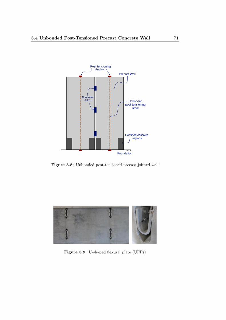
3.4 Unbonded Post-Tensioned Precast Concrete Wall 71
Figure 3.8: Unbonded post-tensioned precast jointed wall
Figure 3.9: U-shaped flexural plate (UFPs)

72 Unbonded Post-Tensioned Concrete Shear Wall
One of the objective of this program was the design, modeling and testing
of an unbonded post-tensioned precast jointed wall. The lateral resisting
system is composed of two vertical precast wall panels placed side by side.
Shear sliding occurs at the vertical joint between them. Each wall may be
composed by several elements stacked one above the other or by a single ele-
ment and it is vertically post-tensioned from the roof level to the foundation.
The tendons may be placed at the edge or at the middle of the wall. The
second option is preferable because it induces the least average tendon elon-
gation. The tendons are designed to remain elastic for the design drift, and
therefore for the design gap opening. The vertical joint presents several shear
connectors that dissipate energy by yielding. PRESSS building test contains
the U-shaped Flexural Plates, initially proposed by Kelly et al. (1972), even
if other connector types may be considered. A relative vertical displacement
occurs between adjoining panels, as the walls rotate and the base crack causes
uplift. When the ends of the UFP are subjected to a relative displacement,
the semi-circular section rolls along the plate and dissipate energy where the
radius of curvature changes from straight to curved and vice versa [1].
Unbonded Post-Tensioned Hybrid Wall
The term “hybrid” reflects that a combination of unbonded post-tensioning
steel and traditional mild steel reinforcing bars is used for lateral resistance
across the wall base joint. The hybrid wall behaves as a single unbonded
PT precast concrete wall: the base joint opens up and the tendons elongate
between their anchors. The mild steel reinforcement undergoes tension and
compression yielding, providing a source for energy dissipation during seismic
event. For these reasons it is called energy dissipation steel, or just ED steel.
The bars are normally debonded over a short length of the base wall panel

3.4 Unbonded Post-Tensioned Precast Concrete Wall 73
Figure 3.10: Unbonded Post-Tensioned Hybrid Wall: general layout and dis-
placed configuration
in order to reduce the strain demand and prevent fracture of concrete while
the steel elongate. On the other side the ED steel is cast into the foundation.
The main advantage of this system is that while the seismic response of a
hybrid wall is fundamentally different than a traditional reinforced concrete
wall, its construction components are conventional and standardized, not
requiring special manufacture or expensive devices like viscous dampers. On
the other hand, the ED steel inside the precast concrete panels can not be
so easily repaired or replaced in case of fracture as external devices such as
the U-shape flexural plates.
Unbonded Post-Tensioned Precast Concrete Walls With Supple-
mental Damping Devices
Another way to dissipate energy could be using additional damping devices,
that could be viscous dampers or friction dampers. A viscous damper is a
mechanical device which softens the imposed displacement, turning it into a

74 Unbonded Post-Tensioned Concrete Shear Wall
(a) general layout (b) wall panel deformed shape
Figure 3.11: Unbonded post-tensioned precast walls with spread viscous dampers
viscous friction. The resulting viscous force is proportional to the velocity,
and it has opposite sign to the applied force. The resultant force will be
smaller than the force applied to the device, and consequently the motion
decreases. In particular a fluid viscous damper device dissipates energy by
pushing fluid through an orifice, producing a damping pressure, therefore a
damping force.
Friction dampers are designed to have moving parts that slide over each
other during a strong earthquake. When the parts slide over each other,
they create friction which dissipates some of the energy from the earthquake
that goes into the building. For example the pall friction dampers consist of
a series of steel plates which are clamped together with high strength steel
bolts and allowed to slip at a predetermined load. These plates are treated
in a particular way to develop friction. Usually friction dampers are simpler
and less cheap than viscous dampers.
Kurama in [7] proposed unbonded post-tensioned precast concrete walls

3.4 Unbonded Post-Tensioned Precast Concrete Wall 75
in which the supplemental energy dissipation system is made with linear fluid
viscous dampers placed inside diagonal braces anchored to the precast wall
at one end and to a column on the other end. The unusual characteristic of
this system is that it uses not only the panel-to-foundation joint, but also
the panel-to-panel joint. Each gap opening in the wall creates a relative
displacement between the two ends of the braces and therefore velocity in
the dampers. Interesting from the engineering point of view, this solution
could not fit architectural requirements.
The use of friction and viscous damping devices improve the performance
of self-centering systems providing the necessary energy dissipation. In an
hybrid wall the presence of mild reinforcement and PT tendons at the base
wall create congestion problems between all the components. Therefore in
some cases construction issues imposed the use of external damping devices
instead of bars inside the concrete. On the other hand, these systems repre-
sent a specialized, relatively unfamiliar and therefore expensive technology.
Another possible configuration of self-centering wall with viscous damping
devices will be presented in Chapter 6.
Propped Rocking Wall
In the San francisco Bay Area several buildings underwent seismic retrofitting
using propped shear wall systems, monolithic cantilever walls propped with
friction dampers (Wolfe et al. 2001). Fathali (2009) proposes an enhance-
ment of the existing propped shear wall, called propped rocking wall (PRW),
which consists of a post-tensioned concrete wall which is propped near its
top by multistory diagonal braces. These long braces can incorporate hys-
teretic dampers and they are supported by the floor slabs of the building
to reduce buckling instability. Unbounded PT bars are installed at the cen-

76 Unbonded Post-Tensioned Concrete Shear Wall
Figure 3.12: Propped rocking wall: general layout and deformed shape, [11]
ter of the wall section to minimize axial strains and prevent steel yielding
resulting from large lateral drifts. Nicknam at al. [11] developed a direct
displacement-based design (DDBD) methodology for PRWs.
3.5 Unbonded Post-Tensioned Hybrid Wall
After looking at all the possible configurations of unbonded post-tensioned
precast concrete walls with different energy dissipation systems, we focused
on the hybrid solution. Fig. 3.10 shows the elevation and of a typical un-
bonded post-tensioned hybrid wall. It consists of vertical panels stacked one
over the other. The desired nonlinear behavior under lateral load is governed
by the opening of gaps along the horizontal joints, in particular the one
between the wall and the foundation. High strength post-tensioning (PT)
steel and mild steel reinforcement cross the base joints and provide enhanced
seismic characteristic to the wall system. A restoring force that closes the
uplift upon unloading is given by the PT steel, resulting in the ability of the
structure to return toward its original undisplaced position after the seismic

3.5 Unbonded Post-Tensioned Hybrid Wall 77
event. For this reason the strands should remain elastic during the ground
motion and don’t lose their re-centering peculiarity. To protect the tendons
from yielding as the gap opening at the base joint occurs, the initial pre-
stress of the strands fpi usually ranges from 55 to 65 percent of the ultimate
strength of the post-tensioning steel, fpu.
The tendons are covered with corrosion inhibiting coating and encased in
a plastic sheathing and the bond between them and the concrete is intention-
ally prevented. Therefore the strains and stresses of the tendon depend on
the overall deformation of the wall over the unbonded length rather than the
sectional deformations. The use of unbonded tendons allows the wall to suffer
significant lateral displacements without yielding of the high strength steel.
Moreover the PT steel does not transfer tensile stresses into the concrete
and the wall panels remain undamaged without cracking. For this reason
the unbonded post-tensioned solution is preferable to the bonded one.
The mild steel reinforcement is designed to yield in tension and compres-
sion providing inelastic energy dissipation (so it is called energy dissipating
(ED) steel). In order to prevent fracturing of the ED steel and cracking of
concrete while the steel yields, the reinforcement can be isolated from the
concrete by wrapping it with plastic sleeves over a predetermined height near
the horizontal base-panel-to-foundation joint. The amount of mild reinforce-
ment is reduced thanks to the addition of post-tensioning which provides a
significant increase in flexural strength. This results in more compact wall
dimensions with respect to a conventional cast-in-place reinforced concrete
wall. A small amount of mild reinforcement is placed at the upper joints and
avoids gap openings.
The gap opening behavior of the hybrid wall leads to minimal concrete
cracking but localized compression damage should be expected at the toes

78 Unbonded Post-Tensioned Concrete Shear Wall
of the base panel, around which the wall rotates at the base. Under a strong
earthquake, the cover concrete at the wall toes will be damaged and pos-
sibly spalls, but it is acceptable and could be easily repaired if necessary.
However, extended damages of the concrete are unwanted and confinement
reinforcement in the form of closed hoops should be placed at the ends of
the base panel to prevent compression failure of the boundary regions. From
a practical standpoint, these regions could be very congestioned and it is
necessary to have the ED steel and PT steel outside them.
The horizontal joints must ensure shear slip capacity, especially the one
between the wall and the foundation. The prestress, together with the gravity
loads, provide a clamping force which resists shear slip along the horizontal
joints. Usually the joints present plain dry-packed connections with surface
contact and their shear slip capacity is given by the product of the shear
friction coefficient and the compression force acting on them due to gravity
loads and PT force. Previous researches (Foerster 1989) show that a reason-
able value of shear friction coefficient for horizontal connections of unbonded
post-tensioned precast walls could be 0.5. Gap opening due to seismic force
reduces the contact area and the shear slip capacity decreases. In a prop-
erly designed and proportioned hybrid wall, shear slip displacements along
the horizontal connections can be neglected as a result of unbonded post-
tensioning.
Basing on the technologies developed for unbonded post-tensioned precast
hybrid wall, recent studies tried to apply it to cast-in-place concrete walls.
Panian et al.([12], [13]) design the retrofit of buildings that use unbonded
post-tensioned cast-in place hybrid walls as lateral resisting system in Berke-
ley and in general in the San Francisco Bay Area. This technology tries to
blend the self-centering capability provided by the vertical post-tensioning

3.5 Unbonded Post-Tensioned Hybrid Wall 79
with the intrinsic advantages of cast-in-place construction to provide a more
effective and efficient seismic resistance system. There are specific construc-
tion details that differ precast and cast-in-place constructions, but the lateral
behavior of the two systems under seismic loads is analogous.
Figure 3.13: Hybrid PT-CIP wall behavior, [12]

80 Unbonded Post-Tensioned Concrete Shear Wall
3.5.1 Design Assumption
The study of the hybrid wall described above is conducted with two-dimensional
analysis of simple isolated walls, neglecting the three-dimensional seismic
effect. The following assumptions and considerations are made for two-
dimensional analysis and modeling:
1. Seismic forces are in the direction of the wall;
2. Torsional, shear or out-of-plane displacements are ignored and the wall
is subject only to in-plane flexural displacement;
3. The wall itself resists to the entire seismic force in the wall direction;
4. The foundation and the supporting ground are rigid;
5. Out-of-plane instability of the wall is not modeled;
6. Anchorages of the tendons remain fully effective during the seismic
response of the wall;
7. The interaction between the wall and the floor diaphragms is limited
to the lateral forces that each level transfers to the wall;
8. In case of precast wall, there is no panel-to-panel gap opening.
3.5.2 Seismic Design Approach
The best way to design a lateral resisting system under seismic loading is a
performance-based design approach, where the designer specify the expected
performance of the structure under a specified earthquake magnitude. For
this reason we need to establish seismic performance levels, and therefore
seismic input levels and building limit states.

3.5 Unbonded Post-Tensioned Hybrid Wall 81
Seismic Performance Levels
ASCE 41, Seismic Rehabilitation of Existing Buildings (2007), recommends
four levels of performance, which are the Collapse Prevention, the Life Safety,
the Immediate Occupancy and the Operational Building. The performance
levels are selected based on the level of post-earthquake service that needs
to be provided.
• The Operational Building performance level assumes that the
building sustains minimal or no damage to their structural and non-
structural components and it is able to continue its normal operations
after the seismic phenomenon.
• The Immediate Occupancy performance level requires that the
structure would be in operation right after a major earthquake without
loss of lives. It is usually assigned to essential facilities like control
buildings, hospitals or police centers. Buildings that meet this building
performance level are expected to support limited structural damage
and only minor damage to their nonstructural elements. Although
immediate occupancy is possible, some repair of utility services may be
necessary before the building full functionality is restored.
• The Life Safety performance level reduces the risk to life loss or
serious injury to the plant personnel or public during the design earth-
quake. This performance level includes extensive damage to both struc-
tural and nonstructural components of the structures but some margin
against total or partial collapse still remains. Repairs may be required
before re-occupancy, though in some cases they are so widespread that
it may not be cost effective.

82 Unbonded Post-Tensioned Concrete Shear Wall
• The Collapse Prevention performance level describes a post-earthquake
condition in which the entire building is tending toward total collapse
but it already has safety margin in order to avoid significant loss of lives.
However, many buildings designed to meet this performance level may
lead to complete economic losses and should be demolished.
Seismic Input Levels
Earthquake records for a specific site where the building will rise are scaled
to two different seismic input levels. These levels are related to the seismic
hazard of that geographic area, so to the probability that an earthquake of
the same magnitude will occur during the life of the structure. The Design
Basis Earthquake (DBE) is defined to have a 10% probability of being ex-
ceeded in 50 years, corresponding to 475 years return period. Instead the
Maximum Considered Earthquake (MCE) is defined to have a 10% chance
of exceeding in 250 years and it is usually defined in the common practice as
3/2 of the DBE. The Life Safety performance level and the Immediate Occu-
pancy performance level are the target level for the DBE, while the Collapse
Prevention performance level is the target level for the MCE.
During the design phase these input levels can be taken into account in
terms of response spectra or ground motion time histories, depending on
the type of analysis the designers are conducting. If they are performing a
static equivalent lateral force procedure, the distribution of the lateral loads
over the height of the building is determined through the well-known Force-
Based Design method (FBD) or through the Direct-Displacement-Based De-
sign method (DDBD). It is important to notice that these two methodologies
lead to lateral forces that could be very different in some kind of structures,
as we saw in the previous chapter. For this reason it is interesting to un-

3.5 Unbonded Post-Tensioned Hybrid Wall 83
derstand which static-equivalent method brings to more realistic values, in
order to find a solution that minimize the size of structural components and
the material quantities for reaching the same performance goal.
Building Limit States
The building limit states should consider the entire construction, including
limit states for the unbonded post-tensioned hybrid wall, the moment re-
sisting frame (if present), the gravity load resisting system, and also the
non-structural components. As regards the hybrid walls, the most important
limits states could be:
1. Gap opening at the base;
2. Spalling of cover concrete at the base;
3. Yielding of the post-tensioning steel;
4. Crushing of the confined concrete;
5. Shear slip along the horizontal joints.
The wall design capacities should therefore satisfy these limit states, which
are associated to different performance levels. The wall demands are summa-
rized by two parameters: the base shear demand and the roof drift demand.
For the DBE we define the design base shear demand Vwd and the design
roof drift demand ∆d, while the maximum base shear demand Vmax and the
maximum roof drift demand ∆max correspond to the MCE.
3.5.3 Design Objectives
Before developing an analytical procedure to design an unbonded post-tensioned
hybrid wall, we need to define the expected behavior of the structure in the

84 Unbonded Post-Tensioned Concrete Shear Wall
different performance levels considered. The enhanced properties of the self-
centering structures, described above, allow to design structures that achieve
the Immediate Occupancy performance level under the design basis earth-
quake and the Collapse Prevention performance level under the maximum
expected earthquake. The goals of this research is to understand which anal-
ysis methodology between common FBD and DDBD is suitable for design
unbonded post-tensioned hybrid walls and to study the response of differ-
ent possible configurations. We are not interested in a full-detailed design
procedure, which is already present in literature. For this reason we develop
just a preliminary design of the structure in order to assess the re-centering
capacity and the energy dissipation of the wall subject to the design level
ground motion. So we will focus on the Immediate Occupancy performance
level, that is reached if:
1. The wall behavior is approximately elastic, but nonlinear;
2. Non-linearity is primarily due to gap opening at the base;
3. Shear slip at the base horizontal joint does not occur;
4. No residual displacement of the wall after the ground motion occurs;
5. PT steel remains in the linear-elastic range;
6. ED steel yields during the seismic event;
7. Wall panels remain linear-elastic, behaving as a rigid body, except for
the wall toes;
8. The non-linearity of concrete in compression occurs only at the wall
toes, where the cover concrete is on the verge of spalling;

3.5 Unbonded Post-Tensioned Hybrid Wall 85
9. Lateral load strength and gravity load strength of the wall are not
reduced after the earthquake.
3.5.4 Base Cross-Section Design
These considerations provide us all the required tools for developing an ana-
lytical procedure for the design of an unbonded post-tensioned hybrid wall.
The amount of PT steel and ED steel, their location at the cross-section
and the wall dimensions are calculated to satisfy the wall design base forces
(calculated with the FBD or the DDBD). The wall section should have a
symmetric layout and the ED and PT steel should be placed outside the
confined regions at the wall toes.
Sectional behavior
The sectional behavior will be determined through the basic concepts of pre-
stressed concrete mechanics, with only one main difference: steel behavior
doesn’t follow compatibility, but kinematic. In fact a gap opens at the base
and neither the PT steel nor the ED steel are bonded to the concrete and
therefore the hypothesis of perfect adherence between steel and concrete is
no more valid. We have to use kinematic considerations due to base sec-
tion rotation, that creates a relative displacement between the two ends of
the debonded mild reinforcement and the two anchorages of the PT steel.
Since the wall panel behaves approximately as a rigid body, the base section
rotation is equal to the roof drift θd, calculated as the ratio between the de-
sign roof displacement ∆d and the wall height hw. Fig. 3.14 shows the base
horizontal joint and the displaced configuration of an hybrid wall with PT
tendons less eccentric than the ED bars, but the following design procedure
is still valid if the section has a different layout. The steel areas are consid-

86 Unbonded Post-Tensioned Concrete Shear Wall
Figure 3.14: Base joint: exaggerated deformed shape at ∆d
ered lumped, respectively, in two areas placed symmetrically respect to the
centerline. We can determine the elongation of the ED bars δs,l and δs,r and
the elongation of the PT steel δpt,l and δpt,r, where l and r define respectively
the displacement on the left and on the right of the centerline.
δs,l = θd
(lw2− xn + es
)(3.1a)
δs,r = θd
(lw2− xn − es
)(3.1b)
δpt,l = θd
(lw2− xn + ep
)(3.1c)
δpt,r = θd
(lw2− xn − ep
)(3.1d)
where:
lw is the wall length;

3.5 Unbonded Post-Tensioned Hybrid Wall 87
xn is the neutral axis length, i.e the contact length between wall and foun-
dation;
es is the eccentricity of the ED bars from the wall centerline;
ep is the eccentricity of the PT tendons from the wall centerline.
In literature the relative location of ED and PT steel is a very discussed topic.
Panian et al. in [13] say that it is advantageous to keep the tendons grouped
closely in the middle of the wall to minimize strains resulting from large
lateral drifts and prevent yielding. On the other hand, Smith et al. in [23]
assert that placing the mild reinforcement close to the centerline assures that
all the bars yield minimizing the steel area required to achieve the expected
energy dissipation. The value of es and ep should be carefully selected in the
design phase and could substantially modify the final amount of steel. The
relative strains can be calculated with the uniaxial strain equation. The total
strand strains are the sum of the gap opening strains and the initial strains
due to prestress. So:
εs,l =δs,lls
(3.2a)
εs,r =δs,rls
(3.2b)
εpt,l =δpt,llpt
+fpiEp
(3.2c)
εpt,r =δpt,rlpt
+fpiEp
(3.2d)
where:
ls is the debonded length of the mild reinforcement;
lpt is the unbonded length of the post-tensioned tendons, equal to the wall
height hw;

88 Unbonded Post-Tensioned Concrete Shear Wall
Figure 3.15: Stress-strain relationship for PT strands (on the left) and ED bars
(on the right)
fpi is the initial prestress, that ranges from 55 to 65 percent of the ultimate
strength of the post-tensioning steel, fpu;
Ep is the elastic modulus of the strand.
The calculated strains can be used to determine the stresses from an assumed
stress-strain relationship for the steel. They are called σs,l, σs,r, σpt,l and
σpt,r. In this project the perfect elastoplastic behavior is used for the ED
bars, while the PT strands are assumed bilinear elastic, but more accurate
constitutive laws could be used without modifying the method. Since the
only reason why the reinforcement has been positioned within the section is
to dissipate energy, at least one of the two lumped areas should yield. The
relative wrapped length is selected in the design in such a way that the ED
bars reach the yield strength fy. Note that these equations are based on the
approximation of neglecting the flexural and shear deformation of the wall
panels over the height of the structure. In this way the process tends to
overestimate the steel strains and thus the stresses.

3.5 Unbonded Post-Tensioned Hybrid Wall 89
Figure 3.16: Base joint: free body diagram at ∆d
Equilibrium Equations
In order to determine the ED and PT steel areas needed, to satisfy the design
base moment demandMwd and the design axial loadNwd due to gravity loads,
simple equilibrium equations of the free body diagram (see Fig. 3.16) at the
wall base are needed. Mwd is calculated from the distribution over the height
of the wall of the design shear force Vwd due to lateral forces.
Cd = 0.85 f ′c tw β1 xn (3.3)
Cd = Nwd + As (σs,l + σs,r) + Apt (σpt,l + σpt,r) (3.4)
Mwd
φf= Cd
(lw2− β1
xn2
)+ As (σs,l − σs,r) es + Apt (σpt,l − σpt,r) ep (3.5)
where:
Cd is the total concrete compressive stress resultant;
f ′c is the compressive strength of the unconfined concrete;

90 Unbonded Post-Tensioned Concrete Shear Wall
tw is the wall thickness;
β1 is the parameter that relates the neutral axis length xn and the relative
rectangular concrete compression stress block;
As is the lumped ED steel area;
Apt is the lumped PT steel area;
φf is an reduction factor that ACI 318 recommend equal to 0.9.
The formulas imply that the steel areas are placed symmetrically respect
to the wall centerline. They could be further simplified considering a mean
value of the steel stresses:
σs,m =σs,l + σs,r
2(3.6)
σpt,m =σpt,l + σpt,r
2(3.7)
The equilibrium equations can be written as:
Cd = 0.85 f ′c tw β1 xn (3.8)
Cd = Nwd + 2Asσs,m + 2Aptσpt,m (3.9)
Mwd
φf= Cd
(lw2− β1
xn2
)(3.10)
Note that the compressive strength of the unconfined concrete is con-
sidered, even if boundary regions are confined. This limitation protects the
concrete from possibles premature cracking, that should be avoided for the
selected performance requirements.

3.5 Unbonded Post-Tensioned Hybrid Wall 91
Proportioning ratio
One of the key aspect for an efficient design of an hybrid wall is the pro-
portioning between the yielding contribution, which is responsible for the
energy dissipation of the system, and the self-centering contribution. In fact
unbonded post-tensioned precast walls are excellent self-centering systems,
able to resist to an earthquake with minimal structural damage. However,
the walls don’t have the ability to dissipate energy which is subject to the
structure during a ground motion, because the response is nearly elastic. Sup-
plemental energy dissipation elements are therefore needed but they should
not compromise the favorable rocking response and the re-centering tendency
of the system. This design criteria could be summarized as the ratio between
the yielding components and the elastic restoring components. In terms of
base flexural resistance, it means:
κd =Myielding
Mrestoring
(3.11)
The influence of κd on the overall response of the generic self-centering system
is well described in figure, representing the idealized flag-shaped hysteretic
loop describes in Section 3.3.2. The value of the ratio determines the amount
of dissipated energy and the re-centering ability of the system. The nominal
base moment strength of an unbonded post-tensioned hybrid wall can be seen
as the sum of three components, Mwn, Ms and Mpt, representing respectively
the contributions of applied axial loads, the wall mild steel reinforcement and
PT tendons. Thus the parameter κd, proposed by Kurama and called “ED
steel moment ratio” is defined as:
κd =Ms
Mpt +Mwn
(3.12)
Referring to Fig. 3.16, the moment equilibrium around the center of com-
pression allows us to rewrite Eq. (3.13). If both the ED steel areas yield, it

92 Unbonded Post-Tensioned Concrete Shear Wall
Figure 3.17: Idealized flag-shaped hysteretic loop
become:
κd =2Asfy
2Aptσpt,m +Nwd
(3.13)
Design steps
An appropriate value for κd should be selected for design. If the yielding
contribution is too small (i.e., κd ratio is too small), then the system doesn’t
provide adequate energy dissipation. Conversely the self-centering capability
of the wall may be too small and thus it may not be sufficient to close the
gap opening at the base joints after the seismic event, if the κd ratio is too
large. Kurama suggested to use values of the ED steel moment ratio that
ranged from 0.50 to 0.80 to satisfy the required performances and the code
requirements of the ACI ITG.
An iterative process is needed to estimate the flexural steel areas required
at ∆d. An initial value of the neutral axis length can be used to determine the
ED steel and PT steel elongations using the displaced configuration and the
selected location of the bars (es) and tendons (ep) from the wall centerline.

3.5 Unbonded Post-Tensioned Hybrid Wall 93
Then the stresses σs,l, σs,r and σpt,m are calculated with the selected unbonded
length (ls and lpt) and the selected stress-strain relationship. ls must be
selected in such a way that at least one of the lumped areas yield. The
required Apt and As can be found by solving Eqs. (3.4) and (3.13) for an
assigned value of κd. Finally if Eq. (3.5) is satisfied, the trial value of xn
is correct, otherwise it must be changed and the process starts over until
convergence.
For lumped steel areas, the design is made without iterations and xn is
solved directly from Eqs. (3.8) and (3.10). The steel areas are computed
using Eqs. (3.9) and (3.13), after the definition of their relative strains and
stresses.

94 Unbonded Post-Tensioned Concrete Shear Wall

Chapter 4
Model Validation
4.1 Introduction
The objectives of this chapter are to develop an analytical model to validate
the design strength and to see if the wall reproduces the expected behavior.
Another purpose of this research is to understand which seismic methodology
between FBD and DDBD results to be more efficient in terms of strength in
order to reach the target performance of the structure. Since there was no
possibility to verify our results with a test building, in the present research
some models already present in literature have been studied in details with
the attempt to reproduce their results. Most of them use finite element
softwares that are not usually present in structural firms and therefore their
results are not so easily applicable to real case study, and result to be relevant
only in the research field. On the other hand, unbonded post-tensioned
precast shear-walls already built do not have a well detailed analytical design
procedure and their structures were designed using high-performance finite
elements softwares. It appears clear that the use of high-performance analysis
is not convenient in terms of time for the preliminary design of structures.

96 Model Validation
The most important research in the analysis of unbonded post-tensioned
precast shear wall is the phase III of the PRESSS research program and it
is the culminating part of the entire project (already mentioned in Chap-
ter 3). In this phase a five-story precast concrete building has been de-
signed, erected and tested under simulated seismic loading. The structure
presented unbonded post-tensioned jointed precast concrete walls in one di-
rection, and a frame system in the other one. Focusing on the wall system, it
has been designed with both the Force-Based and the Direct-Displacement-
Based methodologies to define the required strength at each level. Later,
the post-tensioned tendons and the energy dissipation devices have been de-
signed. The intent of the work was to create an analytical model whose
results could match the experimental one found with a 60 percent scaled
building.
After a brief summary of previous work, in this chapter the PRESSS re-
search is studied in detail as a prototype in order to fully understand how
an unbonded post-tensioned jointed precast concrete wall has been modeled.
Later the same wall system is modeled using a well-known and commercially
available finite element software like ETABS 2015, highlighting the problem
encountered during the implementation and the advantages derived by its
utilization. Understood how to model it, the methodology can be applied
to different configurations of walls. This will be part of the next chapter,
where different configurations of enhanced lateral load resisting systems with
unbonded post-tensioned walls will be modeled in order to verify that the de-
sign procedure developed in previous chapters is able to provide well designed
structures.

4.2 Literature Review 97
4.2 Literature Review
Over the past few years, research teams and engineering firms tried to model
self-centering walls with unbonded post-tensioned tendons with different en-
ergy dissipation devices. Principally fiber element models have been created,
because in this manner a reasonably accurate model can be developed using
only uni-axial stress-strain models for the various components of the lateral
resisting system. All the fiber element models present in literature are similar
to the one proposed by Kurama et al. at University of Notre Dame whose
main features will be summarize later.
The computer program PERFORM-3D (CSI) is specific for performance-
based seismic analysis and has been used for unbonded post-tensioned walls.
This software gives the possibility to model the structural system in all its
details with minor simplifications. For this reason the relative analysis are
very time-consuming, so it becomes very difficult and inefficient to implement
the model considering the whole structure.
For example the David Brower Center, situated in Berkeley, CA, has been
designed by the engineering firm Tipping Mar with nonlinear time-response
analysis conducted using Perform-3D [28]. The inelastic flexural behavior of
the post-tensioned walls and frames was modeled with inelastic fiber element
sections applied on three-dimensional finite elements. The behavior of the
unbonded tendons is achieved by connecting them only to the wall elements
at the location of the actual anchorages, so the top and bottom of the wall.
The engineers used the model not just as a verification tool, but they also
designed the structure with it.

98 Model Validation
(a) (b)
Figure 4.1: Examples of models developed by University of Notre Dame: (a) is
the finite element model, (b) is the fiber element model
4.2.1 Models developed by University of Notre Dame
A research team leaded by Kurama and Smith in University of Notre Dame,
Indiana, is developing many studies on hybrid precast wall systems in seismic
regions. During the investigations the group proposed 2 different analytical
models that can be used for the analysis of precast concrete shear walls with
unbonded post-tensioning tendons and mild steel that dissipates energy [24]
[23]. Both of them have interesting features, but the main drawback is that
their way of modeling makes it difficult to develop an analytical model to
look at the whole structure and not only at the lateral resisting system. A
brief description of the two models is provided below.
Finite Element Model
A simplified finite element model was created using ABAQUS (Hibbitt et al.
2009) and can be used for pushover analysis and to analyze the local stresses
in case of perforations in the wall panels. 3D eight-node stress/displacement

4.2 Literature Review 99
solid elements are used for the concrete of the wall panels and the foundations
and their behavior is linear elastic in tension, so that the steel reinforcement
inside each wall is considered. It assumes that the amount of ordinary rein-
forcement is enough to guarantee the limitation of cracks inside the concrete.
Regarding the wall toes, the confinement reinforcement is not explicitly mod-
eled but rather represented by incorporating the effect of the confinement on
the stress-strain relationship of the concrete in compression, following the
Mander theory.
The PT steel as well as the ED steel across the base joints and the panel-
to-panel joints are modeled with 3D eight-node stress/displacement truss
elements. The ED steel trusses are partitioned into bonded regions, where
they are constrained with the wall solid elements, and unbonded regions
that are not embedded instead. An initial tension force in the PT trusses
simulates the initial prestress.
The gap opening is allowed thanks to “Hard contact” surfaces at the
horizontal joint and the shear slip depends on the properties of these surfaces.
Detailed Fiber Element Model
The fiber element model using DRAIN-2DX (Prakash et al. 1993) was cre-
ated for nonlinear reversed-cyclic and dynamic analysis. The axial-flexural
behavior of the wall panels is reproduced using fiber beam-column elements,
while the foundation is assumed to be fixed. The effect of gap opening at
the base joint is modeled setting to zero the tension strength of the concrete
fibers over the height of the confined concrete at the wall toes. The remain-
ing height of the wall panels is linear-elastic in tension and the cracks in the
concrete are considered negligible.
The PT steel and the ED bars are modeled with truss elements. The ends

100 Model Validation
of the truss elements are kinematically constrained to the corresponding fiber
element nodes for the wall panels at the same elevation. An initial tension
force in the truss elements simulates the initial prestress in the PT tendons.
The stiffness of the PT strands should be reduced compared to the actual
material properties, to take into account the concrete deformations at the
anchorage regions. So the researchers proposed to reduce the elastic stiffness
of the PT trusses by a factor of 0.75.
Similar to the finite element model, the confinement reinforcement is not
explicitly modeled, but only in its effects on the stress-strain relationship of
the concrete in compression.
4.3 The PRESSS Research Project
The Precast Seismic Structural Systems (PRESSS) research program started
in 1991 and was sponsored by the National Science Foundation, the Pre-
cast/Prestressed Concrete Institute and the Precast/Prestressed Concrete
Manufacturers Association of California with two main purposes [27]:
• to define design recommendations for better performances of precast
concrete structures in seismic region;
• to discover new material, design concepts and technology for precast
concrete during an earthquake to stand out its peculiarity;
The project could be divided in 3 different phases. Phase I focused on the
identification of the precast building system, among the existing ones, which
has better response under a ground motion. Later, phase II studied different
ductile connections and developed design procedures for precast concrete
buildings; finally the third phase executed the design, erection and testing of a

4.3 The PRESSS Research Project 101
five-story precast concrete building providing the definition of detailed design
recommendations for the implementation of the present building codes. The
precast wall panels was evaluated as a part of the first phase, its results and
developments were then tested during Phase II.
The project culminated in 1999 with a five-story precast concrete building
that was erected and tested under simulated seismic loading at the UCSD
Charles Lee Powell Structural Laboratory (San Diego, California). For prac-
tical purposes, the test building was a 60% scaled version of the designed one.
The design of the structure was performed comparing the direct-displacement
based procedure and the force-based one, with the aim to sustain a target
drift of 2% under a design level ground motion. The PRESSS test building
presented two different seismic resisting systems in the two directions of the
structures: a moment resisting frame in one direction and unbonded post-
tensioned jointed precast concrete walls in the other direction. An analytical
model was then developed in order to predict the results found by tests,
using Ruaumoko software, developed at the University of Canterbury (New
Zealand) and specialized on time history non-linear analysis of structures
under seismic loading.
In this research a well-detailed description of the test building, including
structural dimensions, material properties and applied load (both vertical
and horizontal), is present, as well as the definition of the analytical model
in all its part. All these data are fundamental in order to have the assurance
that the created model will be correct and accurate compared to the real
problem. These studies are useful also to validate the design procedures in
order to define the seismic forces acting on the wall.

102 Model Validation
Figure 4.2: Global view of the test building

4.3 The PRESSS Research Project 103
Table 4.1: PRESSS test building scale factors, [3]
Quantity Scale Factor
Length 0.6
Mass 0.63
Time/Period 0.6
Stress 1.0
Acceleration 1/0.6
Force 0.62
Moment 0.63
Damping 0.62
4.3.1 Building Description
The present Section is not meant to be a detailed design report of the
PRESSS test building, that could be easily found in literature ([3] [10] [26]
[27]) , but just an overview of the structural features relevant for the present
research. In reports written by the PRESSS research program, all the quanti-
ties are present according to the United States customary units, so for a more
precise study, they will be shown both in International System of Units (SI)
and in United States Customary System (USCS). The prototype building is
100 ft × 200 ft in plan (30.48 m × 60.96 m) with equal story heights of 12 ft
6 in (3.81 m) and 25 ft (7.62 m) bay length, as shown in Fig. 4.3. The lateral
load resistance is developed by moment-resisting frames in one direction of
response and shear walls in the other direction.
Since there was not enough space at the UCSD Powell Lab, a 60% scaled
version of the building was erected. The quantities were therefore scaled
themselves according to Table 4.1. Therefore the test building consists of 2
bays x 2 bays in plan of 15 ft (4.57 m) span each and it has pretopped double
tee planks as flooring system for the first three floors, while in the upper two
floors topped hollow-core panels are used, as shown in Figure 4.4.

104 Model Validation
Figure
4.3:
Flo
orp
lanof
the
prototy
pe
bu
ildin
g
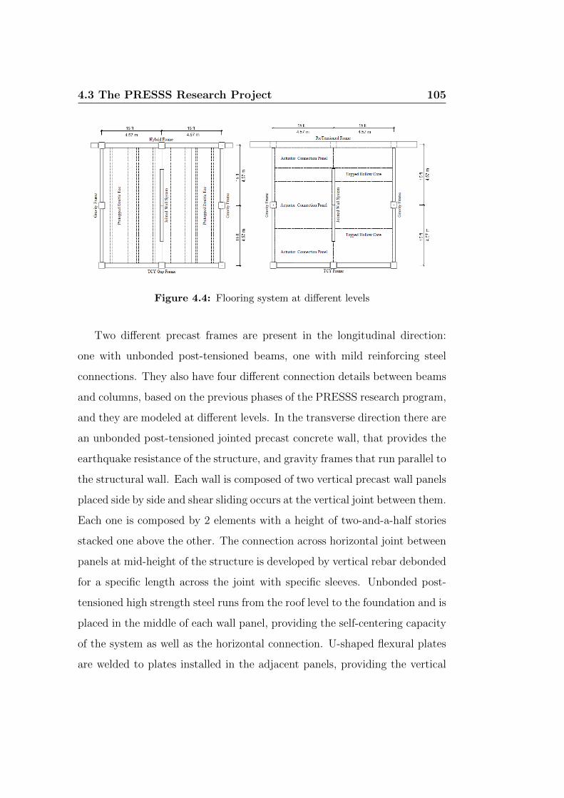
4.3 The PRESSS Research Project 105
Figure 4.4: Flooring system at different levels
Two different precast frames are present in the longitudinal direction:
one with unbonded post-tensioned beams, one with mild reinforcing steel
connections. They also have four different connection details between beams
and columns, based on the previous phases of the PRESSS research program,
and they are modeled at different levels. In the transverse direction there are
an unbonded post-tensioned jointed precast concrete wall, that provides the
earthquake resistance of the structure, and gravity frames that run parallel to
the structural wall. Each wall is composed of two vertical precast wall panels
placed side by side and shear sliding occurs at the vertical joint between them.
Each one is composed by 2 elements with a height of two-and-a-half stories
stacked one above the other. The connection across horizontal joint between
panels at mid-height of the structure is developed by vertical rebar debonded
for a specific length across the joint with specific sleeves. Unbonded post-
tensioned high strength steel runs from the roof level to the foundation and is
placed in the middle of each wall panel, providing the self-centering capacity
of the system as well as the horizontal connection. U-shaped flexural plates
are welded to plates installed in the adjacent panels, providing the vertical

106 Model Validation
connection between them, and thus increasing the lateral resistance. They
also dissipate energy thanks to the relative displacement of the two ends of
the device. The wall panels are 9 ft (2.74 m) wide and 8 in (20.3 cm) thick.
4.3.2 Wall Lateral Resisting System
The wall should remain elastic during tests, so it is significantly reinforced
and it presents spiral confinement at the base toes in order to sustain the high
compressive stresses at maximum drift. The foundation is considered rigid,
with high strength bars that run horizontally on it. High strength fiber rein-
forced grout are used at the base-panel-to-foundation joints, to avoid shear
slip. The centerline of each panel collects 4 unbonded tendons (Dywidag
coupled thread bars) of 1 in (25.4 mm) diameter. Bolted to anchor plates
which are imbedded into the foundation, these bars should remain elastic up
to the 2% drift design limit. Therefore each bar is post-tensioned to a force
of 41 kips (182.4 kN). In this way the wall has re-centering capacities after
the design ground motion. In order to limit the deformations of the flooring
system when the wall rocks during the seismic event, specific connections
are needed to transfer the horizontal loads, but not the vertical ones. The
weight of the wall, the weight of its tributary area at each floor and the
post-tensioning force are considered as concentrated loads at the base of the
wall. In this manner it is possible to model the restoring force that pulls
the structure back to the initial configuration. Adjacent panels are then cou-
pled with U-shaped flexural plates (UFPs) placed along the vertical joints
between them. Moreover these devices assures energy dissipation capacity
to the system, as they yield thanks to the relative vertical displacement of
the ends of the plates. Welded to imbedded plates in the panels, the semi-
circular section of the device rolls along the plate and dissipate energy where

4.3 The PRESSS Research Project 107
the radius of curvature changes from straight to curved and vice versa.
Figure 4.5: Elevation of the unbonded post-tensioned jointed precast wall, [10]

108 Model Validation
Figure 4.6: Erection of the unbonded post-tensioned jointed precast wall

4.3 The PRESSS Research Project 109
4.3.3 Design Procedure
The required strength of the wall under seismic loads was computed with
both the DDBD method and the FBD method. The value found with the
DDBD resulted to be the optimal one, and thus it leaded the design of
the wall. The FBD reduces the elastic forces generated on the structure
by an R factor in order to take into account the non-linear behavior of the
structure. The R factor used is related to the ductility of the system assuming
an emulation of monolithic concrete behavior. In this way, this procedure
does not capture the specific behavior of the jointed precast system because
its energy dissipation characteristics and its yield displacement profile are
different from the one of a conventional monolithic wall.
The PRESSS building was designed to carry a maximum drift of 2% under
a design level earthquake that follows the 1997 UBC acceleration spectrum
provisions, considering seismic hazard Zone 4 and intermediate soil type Sc,
which corresponds a PGA equal to 0.4 g. The displacement spectra of Ap-
pendix G of the SEAOC Bluebook (PBSE-SEAOC, 1998) were used.
In the DDBD an equivalent viscous damping of 20% was estimated by
the designers. The displacement profile was assumed to be linear along the
height, due to essentially elastic behavior of the wall during the seismic event
as illustrated in Chapter 2. The values resulting from the DDBD procedure
to compute the design base shear are listed in Tab. 4.2. These results consider
the 4 walls composing the lateral resisting system of the prototype building.
In the test building a 60% scale version of only one of the 4 wall system
in the prototype building was modeled. Hence, the design base shear of one
wall is:
2167 · 1
4= 541.75 kips ( 2409.8 kN ) (4.1)
Table 4.3 shows the values of base shear force found with DDBD and

110 Model Validation
Table 4.2: Results from the DDBD procedure
PropertiesParameters
USCS SI
∆d 11 in 0.28 m
Me 41.32 kips/in.s2 7164.66 ton
Te 2.88 sec 2.88 sec
Ke 197 kips/in 34500 kN/m
Vb 2167 kips 9639.30 kN
FBD. This table allows to make a comparison between the forces obtained
with the two methods in the wall direction. The force based design was
applied in accordance with different codes (UBC 94, UBC 97 and NEHRP
97) and in all cases the values provided by this method was higher than the
one estimated by the DDBD method. It is of interest to see that the FBD
method produces a force that was 80-100 % higher than the one produced
by the DDBD method. Reduction of base shear indicates cost saving in the
realization.
Table 4.3: Comparison of the design base shear obtained from DDBD and FBD,
[26]
Design Method CodeBase Shear
USCS SI
DDBD PBE-SEAOC 2167 kips 9639 kN
FBD
UBC 94 3900 kips 17348 kN
UBC 97 4333 kips 19274 kN
NEHRP 97 3900 kips 17348 kN

4.3 The PRESSS Research Project 111
In the analysis with FBD different values of Ct and Rw were considered.
For UBC 94 they were Ct = 0.02 and Rw = 6, for UBC 97 Ct = 0.02 and
Rw = 4.5, for NEHRP 97 Ct = 0.02 and Rw = 5.
The prototype building was then tested with a 60% scale building test.
The quantities found with DDBD method were scaled according to Table 4.1.
The values of interest are the design base shear and the floor weight. These
values are interesting for the creation of a validation model that tries to
reproduce the values found with the PRESSS program. The design base
shear of the test building in the wall direction resulted to be:
2167 · 1
4· 0.62 = 195.0 kips ( 867.4 kN ) (4.2)
The weight associated to each floor of the test building was calculated
from the total building weight of 19500 kips:
19500 · 1
5· 1
4· 0.62 = 351 kips ( 1561.3 kN ) (4.3)
The test executed on the wall designed with the DDBD provided also a
validation of this method, as it will be shown in the following sections.
4.3.4 Modeling Assumption
The model of the wall system developed in this work is based on previous
attempts to model this kind of structures, first of all the studies leaded by
Kurama on unbounded post-tensioned precast concrete walls and described
in Sec. 4.2. The model, obtained using the Ruaumoko Software, adopts only
frame elements and spring elements, with different section properties and dif-
ferent elasto-plastic behavior, to represent the various structural components.
The wall is represented also with a column on its right side, representing
the potential unbonded post-tensioning frame, which gives additional lat-
eral resistance to the structures. This column is not modeled in the present

112 Model Validation
research, so it will not be described in the following part. The floors are
modeled as lumped masses located at the same elevation, suggesting the hy-
pothesis that each level behaves as rigid diaphragm. These represent the
seismic masses used for the definition of the horizontal forces due to the
earthquake. The vertical loads, computed as the sum of the wall self-weight,
the weight of the floors sustained by the wall and the initial prestress, are ap-
plied as concentrated loads at the base of the panels. As it will be described
later, this procedure assure that the system develops the necessary restoring
force at the base during the seismic event. Finally, the Rayleigh damping
used for the time history analysis is equal to 2.5% for the first mode, and 5%
for the second mode.
Below it is present a full description of the single elements that model the
different components present in the wall seismic resisting system, according
to [3].
Wall Members
The wall member is modeled with 5 frame elements that start from the
base and their length is equal to the story height. The panels are designed
to remain elastic during the earthquake, so the gross section properties are
considered, without taking into account the reduced moment of inertia due
to cracks inside the concrete. As other conclusion of the design assumptions,
the hysteretic characteristic of the wall components are the ones of a simply
linear-elastic element, without energy dissipation nor stiffness degradation.
During the PRESSS research program, experimental tests on materials used
in the test building were conducted and the relative results are present in
different reports. In this manner they could estimate the elastic modulus
and the shear modulus of the precast concrete panels. The global properties

4.3 The PRESSS Research Project 113
Figure
4.7:
Ru
aum
oko
mod
el,
PR
ESS
Sre
por
t

114 Model Validation
can be summarized as below:
Table 4.4: PRESSS test building, wall member parameters
PropertiesParameters
USCS SI
Elastic Modulus E 5200 ksi 35853 MPa
Shear Modulus G 2200 ksi 15168.5 MPa
Cross Section Area 864 in2 5574 cm2
Shear Area 736 ksi 4748 cm2
Moment of Inertia 839808 in4 34955448 cm4
Rigid Links
As shown in Fig. 4.7, the nodes at the base of the wall component have 2
rigid-links that are horizontal and have different length: the outer link is
49.6 in (126 cm) long, while the length of the inner one is 53 in (134.6 cm)
from the centerline of the wall panel. These nodes do not represent the
real size of the wall panels, but they are the centers of compressions of the
wall section calculated with a sectional analysis at a total drift of 2% and
assuming a concrete compressive stress block distribution at the toe of the
wall panels.
The other wall nodes also have rigid links that extends inward, to the
center of the wall. Their modeling as rigid is consistent with the assumption
of rigid diaphragm behavior of the flooring system, because in this manner
the horizontal displacements of the walls are constrained. Between the ex-
tremities of these links there are the UFPs, modeled as springs. To simplify
the model, the energy dissipation devices are not placed in the real location
of the test building, but they are placed one at each floor. So, instead of
having 4 U-shaped flexural plates spread along the vertical joint between the
wall panels for each level, they are only 5. Later it will be described how to

4.3 The PRESSS Research Project 115
model them.
The researchers found some problems in the definition of these elements.
High values of their properties change significantly the stiffness matrix, more-
over the model used to fail and crash during the analysis due by the fact that
Ruaumoko doesn’t have any stability checks of the solution. They fixed the
problem applying to the rigid-link the properties of the stiffest element (the
wall frame) multiplied by 100, putting at zero the shear area, in order to
neglect the shear deformations.
Foundation Springs
As described in Chapter 3, a self-centering wall system allows the formation of
a gap at the joint between wall and foundation when the lateral load applies
an overturning moment on it in order to prevent yielding in the concrete
components. Therefore the foundation must be modeled so that the wall
panel could be able to uplift avoiding the compenetration between the two
concrete elements. This is obtained through the modeling of compression-
only elements that have no resistance when the gap opening occurs but that
provide the concrete resistance when the wall and the foundation are in
contact. Hence, the researchers used springs with bi-linear elastic hysteretic
characteristics with different behavior in tension and compression, as shown
in Fig. 4.8. The foundation springs are zero weight elements acting only
in the vertical direction, placed at the external and internal nodes of the
base rigid links. For the moment the focus is on the force reaction that the
foundation apply to the wall panels and not on the displacements, so the
springs extend conventionally for 3 in (7.62 cm) below the base.
Initially the elements have a linear-elastic behavior, with stiffness k equal
for positive and negative forces, after that they deform with zero stiffness.

116 Model Validation
Figure 4.8: Foundation spring hysteretic behavior
The point of discontinuity is almost null in tension (0.1 kips, i.e. 0.45 kN) and
a high value in compression, equal to 800 kips (3558.6 kN) in order to ensure
elastic response. The stiffness instead is the one corresponding to a deflection
of the foundation of 0.02 in (0.05 cm) for a force of 200 kips (890 kN), so
10 000 kip/in (88 512 kN/m).
PT Springs
In the test building post-tensioned tendons run from the foundation up to the
top of the wall. As gap opening occurs at the base-panel-to-foundation joint
during the design earthquake, the strands elongate and provide a clamping
force that can re-center the wall back to its undisplaced position when the
seismic action is removed. The modeling of the PT tendons, fundamental for
a true representation of the advantages related to these kind of structures,
can be done with springs located at the base of the wall panels. These
springs start at the centerline base node of the wall member and are fixed
3 in (7.62 cm) below. In each wall panel 4 tendons prestressed up to a force

4.3 The PRESSS Research Project 117
of 41 kips (182.38 kN) are present, for a resultant force of 164 kips (729.5 kN).
This force, is modeled as a concentrated load applied not in the PT spring
locations, but on the base foundation springs and it provides, with the other
gravity loads, the re-centering effect. Since Ruaumoko gives the possibility
to apply an internal force to an element affecting only its initial deformation
and not the global response, the initial condition of the strands in terms of
stress-deformation due to the prestess was taken into account pre-loading the
PT springs in the vertical direction by 164 kips (729.5 kN). In this manner the
PT springs capture only the increase in the elongation of the post-tensioning
tendons at the center of the walls and not the re-centering behavior.
The researchers chose bi-linear isotropic hardening hysteretic characteris-
tics for the PT springs, with yield value of 375 kips (1668 kN) both in tension
and compression. The properties are summarized in Table 4.5, where the
bi-linear factor is the ratio between the elastic stiffness and the slope of the
hardening segment. They are based also on experimental investigations on
Dywidag bars used in the test building. Tensile tests resulted in an average
yield stress of 153 ksi (1055 MPa) and an average elastic modulus of 29 000 ksi
(199 948 MPa). The elastic stiffness kPT is therefore calculated as:
kPT =Ep · Aptlpt
(4.4)
where lpt is the unbonded length of the PT bars, equal to the height of the test
building, Apt is the total area of the strands and Ep is their elastic modulus.
UFP Springs
The U-shaped flexural plates are modeled with spring elements that connect
among them the horizontal rigid links that start from the wall frame inward
the panels. They are rigid in the horizontal direction in order to show only

118 Model Validation
Table 4.5: PRESSS test building, PT springs parameters
PropertiesParameters
USCS SI
Elastic Stiffness 197 kip/in 35052 kN/m
Yield force 375 kips 1668 kN
Bilinear factor 0.02 0.02
Pre-load force 164 kips 729.5 kN
the effects of vertical displacements on the devices. This is consistent with
the assumption of rigid diaphragm behavior of the floor. During the PRESSS
report experimental tests on UFPs were carried out in UCSD to understand
their hysteretic behavior and then how to model it in the analytical model.
The force-displacement relationship that was found is the solid line in Fig. 4.9,
representative of the characteristics of the dissipating devices actually present
in the PRESSS test building. It is possible to see that the yielding of the
UFP results in a gradual change in stiffness. Moreover, plastic deformations
in one direction affect subsequent plastic response in another direction and
when the UFPs is pulled in tension, for example, it shows a reduction in
compressive strength. This is called Bauschinger effect.
The hysteretic rule that was used in the PRESSS report is the Al-Bermani
Bounding Surface Hysteresis, which is able to model the kinematic hardening
behavior due to Bauschinger effects. As shown in Fig. 4.10, after an initial
constant stiffness k1, the curve has a variable slope till it reaches a line with
stiffness k2 where the curve follows this line. So the hysteretic model define
2 boundary surfaces, both with slope k2: one called F1 that intersects the
elastic straight line in P2, equal to the yielding force Py, and one called F2
that intersects it at a certain fraction of P2. Hence, these two values result

4.3 The PRESSS Research Project 119
Figure 4.9: Force-Displacement relationship of the UFPs, PRESSS report

120 Model Validation
Figure 4.10: Al-Bermani Hysteretic Rule
to be:
P2 = Py (4.5)
P1 = αPy (4.6)
Between these lines the stiffness is variable and its law is:
kT = k1
[1−
(P − F2
F1 − F2
)(1− p)
](4.7)
where p is the ratio between the hardening stiffness and the elastic stiffness,
and thus:
k2 = pk1 (4.8)
The unloading path has the initial slope equal to k1 till it passes through the
first boundary line in the opposite direction, then it works as before.
The test results were then used for the definition of the Al-Bermani, the

4.3 The PRESSS Research Project 121
following values were used:
k1 = 40 kip/in = 7117 kN/m (4.9)
k2 = 0.6 kip/in = 106.75 kN/m (4.10)
Fy = 11 kips = 49 kN (4.11)
The result of this is the dashed line in Fig. 4.9, that correlates fairly well
with the curve obtained by experimental investigations.
The dimensions of the test specimen were different than the one of a UFP
really present in the test building. Therefore, the previous quantities had to
be scaled by a factor equal to 14/3, obtained as the ratio between the cross
sectional areas of the UFPs of the test building per floor level and those of
the test setup. Finally, the UFP springs are zero weight elements with no
strength degradation.
Now it is possible to summarize the properties of the UFP springs used
in the PRESSS model using the Al-Bermani hysteretic rule. As it will be
discussed later, the definition of the UFP springs as defined by the PRESSS
researchers introduces some misunderstanding and inaccuracies. One of them
is that the value of α factor proposed is equal to 0.001, that seems not coher-
ent with the comparison that suggested by them in Fig. 4.9. For consistency
with PRESSS model, in Table 4.6 the α value listed is the one that they
proposed.
Loads and Constraints
The model is vertically constrained thanks to the springs situated at the base
rigid-links, both the UFP springs and the PT springs, that are fixed at the
base. In the horizontal direction instead the right nodes of the rigid links
at the base corresponding to the right extremity of the wall frames are fixed

122 Model Validation
Table 4.6: PRESSS test building, UFP springs parameters
PropertiesParameters
USCS SI
k1 186.6 kip/in 33201.5 kN/m
k2 2.8 kips 498 kN
p 0.015 0.015
Py 51.3 kips 228.2 kN
α 0.001 0.001
from moving in that direction. As the base links are rigid, this assures the
horizontal constrains of the all base and is consistent with the hypothesis
that shear slip is prevented by the design.
The sum of the self-weight of the wall panels, the weight of each floor level
sustained by them, and the initial prestress of the PT tendons, is applied
to the structure as concentrated static loads. The application point of these
forces is at the extreme nodes of the base rigid links in a proportional manner.
Hence, the resulting forces are 120.88 kips (537.70 kN) at the exterior nodes
and 113.12 kips (503.18 kN) at the interior ones.
The seismic masses supported by each floor level have been taken into
account in the PRESSS analytical model as lumped at the wall frame node
locations. These masses act only in the horizontal direction and each one
is equal to 175.50 kips (780.66 kN). They were applied in form of weight
because Ruaumoko subsequently converted them into mass units. It should
be noted that, since length and time are scaled at 60% in the model building,
the acceleration of gravity had to be scaled by a factor 1/0.6, as shown in
Table 4.1.

4.3 The PRESSS Research Project 123
4.3.5 Seismic testing
The PRESSS building is designed by the researchers using the direct-displacement
based approach (DDBD) to carry a maximum drift of 2% under a design level
earthquake that follows the 1997 UBC acceleration spectrum provisions, con-
sidering seismic hazard Zone 4 and intermediate soil type Sc, which corre-
sponds a PGA equal to 0.4 g. As starting point of the DDBD procedure, a
trial value of the equivalent viscous damping coefficient ξ equal to 20% is
used.
The building test was subject to seismic testing in the two main directions
independently. Three different test schemes were used, called:
Flexibility test: a quasi-static loading test in order to compute the stiff-
ness matrix of the test.
Pseudo-dynamic test: the dynamic loads due to earthquake ground mo-
tions are applied quasi-statically thanks to ten on-line controlled hy-
draulic actuator.
IT test: a cyclic loading test using an inverse triangular force distribution
is performed till the maximum displacement achieved in the previous
pseudo-dynamic tests. This analysis in useful to evaluate the equivalent
viscous damping of the structure. Moreover, it gives the possibility to
immediately compare the experimental results with the design proce-
dure, where an inverse triangular acceleration pattern is approximately
used.
The PRESSS reports show the procedure adopted for obtaining suitable
input motions. They derived a design level input motion from the El Centro
record obtained from the 1940 Imperial Valley earthquake [25].

124 Model Validation
4.3.6 Experimental and Analytical Comparison
The PRESSS reports show that the response of the test building during tests
was satisfactory. The wall panels presented no damage after the application
of the design level earthquake to the structure. Minimal cracks in the cover
concrete occurred due to the high compressive strains at the wall toes, but
spalling of the concrete was prevented. Aside from the base, no other damage
to the precast wall panels was noticed. The U-shaped flexural plates present
no fractures and significant yields occurred as assumed during the design
phase. Finally, the post-tensioned tendons provided the self-centering capa-
bility to the lateral resisting system and remained elastic during the design
level ground motion. Among the several results presented by the PRESSS
reports, the present research shows only few of these and the respective pic-
tures presented below have been taken directly from [3].
Fig. 4.11 shows the envelopes of the maximum lateral displacement of
the roof level of the wall under simulated earthquake records, where EQ1,
EQ2 and EQ3 correspond respectively to 33, 50 and 100 and 150 percent
of the design level earthquake. The displacement profiles are very close to
linear, according with the profile used in the design procedure of the DDBD
method. The measured peak roof displacement at EQ3 was 8.28 in, equal to
92% of the design target displacement corresponding to the 2% drift assumed
during the design.
A good indicator of the lateral resistance of the test building in the wall
direction is the relationship between the base moment and the horizontal
displacement of the top floor. The predicted results were obtained through
a pushover analysis, which is usually applied to verify the structural perfor-
mance of a building and estimate the expected plastic mechanisms. Pushover
is a static-nonlinear analysis method where a structure is subjected to gravity

4.3 The PRESSS Research Project 125
Figure 4.11: PRESSS results, test maximum displacement profiles
loading and a monotonic displacement-controlled lateral load pattern which
continuously increases through elastic and inelastic behavior until an ultimate
condition is reached. Lateral load may represent the range of base shear in-
duced by earthquake loading, and its configuration may be proportional to
the distribution of mass along building height, mode shapes, or another prac-
tical means. The load pattern applied by the PRESSS researches to the wall
model was based on the displacement profile used during the DDBD proce-
dure, normalized to the top displacement. Fig. 4.12 shows the comparison
between the predicted results and the experimental ones in terms of base
moment-top displacement relationship. It has been preferred with respect of
the base shear-top displacement relationship because the higher mode effects

126 Model Validation
present in the base shear and floor force time histories do not heavily im-
pact the base moment. Initially, it was used an analytical model composed
Figure 4.12: PRESSS results, pushover curve
only by the wall system but after running the analysis they discovered that
it accounted for about 80% of the response at the maximum displacement
in the wall direction, as shown in Fig. 4.12. The remaining moment resis-
tance was suspected to be due to the moment resistance at the base of the
eight columns in the test building and thus was added to the model. The
result was an increase of about 23% in base overturning moment resistance,
that matches extremely well the experimental evidence expressed by dots in
Fig. 4.12.
Finally, it will be presented the viscous damping calculation performed in
order to verify the equivalent viscous damping coefficient for the wall system

4.4 Proposed Model For Unbonded Post Tensioned ConcreteWalls 127
assumed in the DDBD procedure. If the computed value markedly differs
from the one initially estimated, the design procedure should be performed
again. As already discussed in Chapter 2, the hysteretic viscous damping
coefficient could be calculated thanks to the base shear-top displacement
relationship of a full hysteretic loop, as:
ξhyst =Ah
4πAe(4.12)
where Ae is the equivalent elastic strain energy and Ah is the energy loss per
cycle by the structure.
IT tests were used to have the experimental results of one complete hys-
teretic loop. The values of the hysteretic viscous damping coefficient were
15.78%. Their sum with the assumed elastic damping coefficient equal to 5%
is coherent with the global 20% equivalent viscous damping assumed in the
design procedure.
4.4 Proposed Model For Unbonded Post Ten-
sioned Concrete Walls
In the present research a finite element model of unbonded post-tensioned
concrete walls in different configuration will be developed, in order to under-
stand which one is the most suitable as lateral load resisting system. The
main objectives are:
• to accurately reproduce the nonlinear behavior of the structure includ-
ing gap opening/closing at the base joint and the hysteretic stress-strain
behaviors of the materials;
• to develop modeling guidelines in order to create a model that should
be easily reproduced by a structural engineering firm in the prelim-

128 Model Validation
inary design phase. In this manner the engineers should be able to
compare this solution to a conventional one and understand which one
is the most suitable for the specific case study in terms of building
performance.
For this reasons ETABS 2015 has been used. It is a software package for
structural analysis and design of buildings and it is very common in the
structural engineering field. For example, it is widely used at Skidmore, Ow-
ings and Merrill LLP (SOM), one of the leading civil engineering firm in the
world, that collaborates in this research. Below the individual components
of the proposed model are analyzed separately and the effectiveness of differ-
ent modeling assumptions will be discussed, based on the comparison with
the results of the PRESSS research project. The ETABS Analysis Reference
Manual [29] has been studied to develop the analytical model here proposed.
4.4.1 Wall Members
Modeling the wall panels as frame elements, the PRESSS researchers faced
the problem of how to model the rigid links. In fact, the use of frame elements
gives rise the necessity of understand how to connect the adjacent wall panels
in order to work in a coupled manner preserving the rigid diaphragm behavior
of the floor levels. So they used rigid links starting from the frame nodes
that go inward the wall panels. The same consideration can be made for the
nodes at the base of the frame elements, where rigid elements are required to
link them with the foundation springs placed at the center of compressions.
Researchers admitted that the modeling of those rigid links was initially
a problem, as discussed above. Moreover, the section properties are not
automatically computed by the software but must be calculated by the user
and imposed to the element, creating inconveniences.

4.4 Proposed Model For Unbonded Post Tensioned ConcreteWalls 129
Figure 4.13: Elevation of the proposed model

130 Model Validation
Figure 4.14: Base of the proposed model
In order to solve these complications it was made an attempt of modeling
the wall panels using 2D shell elements that connect two consecutive floor
levels. As before, the wall panels are designed to remain elastic during the
design earthquake, thus a perfect linear-elastic hysteretic behavior is used.
As ETABS 2015 considers this hysteretic rule by default, the assignment
of the correct characteristic of the material that makes up the wall panels is
sufficient for a correct linear-elastic response. The main characteristics of the
material are presented in Table. 4.7. The software gives also the possibility
to restraint the points of a floor level so that it behaves like a rigid diaphragm
assigning the Diaphragm option to these points. Each wall panel is vertically
discretized into 4 shell elements in line with the centerline and the centers of
compressions, in order to have the nodes of the shells at the locations of the
springs. In this way computational errors made by the software are avoided.

4.4 Proposed Model For Unbonded Post Tensioned ConcreteWalls 131
Table 4.7: Proposed Model, wall member parameters
PropertiesParameters
USCS SI
Elastic Modulus E 5200 ksi 35853 MPa
Shear Modulus G 2200 ksi 15168.5 MPa
Section Thickness 8 in 20.3 cm
4.4.2 Modeling of Gap Opening at the Base
The rocking behavior during seismic events of this system is allowed by the
creation of a gap opening at the base of the wall realized with a horizontal
joint between wall and foundation. The correct modeling of this behavior
was one of the first issues that have been observed in the model creation.
Initially the modeling of the rocking behavior was faced through fiber
elements. The foundation was assumed to be fixed, the wall panel constrained
at the base and the gap opening was modeled using concrete fibers at the
wall toes with zero tension strength. Since the non-linear behavior of the
wall is concentrated at the base, the upper part was modeled as linear-elastic
with negligible cracks in the concrete. It has been found that this model
produces non-linear deformations in the wall panels till the first floor level.
It is not in agreement with the real behavior of the system, in which the wall
remains a rigid block. Moreover, the use of fiber elements in ETABS 2015
introduces computational problems if the discretisation of the shell elements
is not almost squared. This limit constrains the positions of the nodes of the
wall panel and does not allow the match between these nodes and the ones
of the PT elements which are placed into design positions.
For these reasons, it has been decided to go towards a model in which
the elements at the base of the wall allow its uplift and maintain the wall
as a rigid block. The direction taken was the one for the creation of specific

132 Model Validation
additional elements that simulate this behavior, and thus it has been decided
to use links elements defined in ETABS 2015. With these elements, the wall
panel is constrained to the foundation through these links, which elongation
could simulate the uplift without causing wall deformations. Moreover, this
choice is in line with the modeling way used in the PRESSS model and allows
the comparison with its results. The characteristics of the link elements are
showed in the following part.
Foundation Links
As it as been said previously, the foundation is modeled in a similar fash-
ion with respect to the model proposed by the PRESSS researchers since
compression-only elements are used in order to model the wall uplift when
the gap opening occurs and the vertical reaction that is present when the
wall is in contact with the foundation. ETABS 2015 gives the possibility to
define Gap elements, that should have the desired characteristics, but the use
of these kind of elements give problems during the analysis and they don’t
work as expected. For this reason it has been decided to model them as
multilinear elastic links as in the PRESSS model and their properties could
be summarized as:
Table 4.8: Proposed Model, foundation link parameters
PropertiesParameters
USCS SI
Stiffness k 10000 kip/in 88512 kN/m
Compression Yield Force 800 kips 3558.6 kN
Tension Yield Force 0.1 kips 0.45 kN
Link Length 3 in 7.6 cm

4.4 Proposed Model For Unbonded Post Tensioned ConcreteWalls 133
4.4.3 Modeling of PT Tendons and the Self-Centering
Behavior
The self-centering capacity of the system is provided by the gravity loads
acting on the wall and by multi-strand tendons running through the wall
panels and the foundation. In order to model this behavior it is essential
that the PT steel and the prestressing force are modeled in the correct way.
According to the initial idea the PT tendons were modeled through frame
elements placed at the centerline of each wall with the application of the pre-
stress by means of thermal deformations. The gravity loads were represented
through the self-weight of the elements composing the wall and with a surface
load applied at each level corresponding to its tributary weight. This option
allows to represent the initial stress in the frame elements but do not take
into account the restoring forces. It was understood that in order to have
the re-centering behavior it is necessary to apply the corresponding quantity
in the way of external forces. Thus, two forces representing the restoring
capacity of the system were applied at the top of the each frame element but
this solution showed other complications. In fact, the concentrated forces do
not follow the deformed shape of the wall in terms of inclination, but only in
term of application point, as it can be seen in Fig. 4.15. The force remains
in the initial direction, i.e in the straight configuration, and thus it does not
reproduce the expected behavior as it becomes a destabilizing force. Its ap-
plication line results to be more external than the centroid of the wall. In
order to solve this disadvantage it was supposed to define a lateral spring that
produces the re-centering effect pulling back the wall. The law governing the
stiffness of the spring should be able to follow the changes of inclination of
the wall thus changing the value of the reacting force.
Another possibility is to model the PT tendons with springs element.

134 Model Validation
(a) (b)
Figure 4.15: Differents model of the re-centering behavior
Spring elements that go from the base to the top of the wall can be used,
substituting in this manner the frame elements previously adopted. The
limitation of this employment is that the springs do not follow the deformed
shape of the wall and remain straight not reproducing the real elongation of
the PT steel. In order to solve this problem a discretisation of the springs
along the height was performed but also this solution did not reproduced the
expected results. Thus, springs with concentrated length at the base were
adopted and the restoring forces were applied at their locations at the base
of the wall panel. This solution is consistent with what carried out by the
PRESSS research program and this solution avoids the transformation of the
vertical forces in destabilizing forces. It was found that such a representation
of the PT strands well reproduce the real elongation of the PT and the self-
centering behavior. The characteristics of these elements representing the
PT steel are summarized in the following part.

4.4 Proposed Model For Unbonded Post Tensioned ConcreteWalls 135
4.4.4 PT Links
The post-tensioning steel is modeled as links at the base of the wall panels and
placed at their centerline. They develop reaction forces due to the elongation
of the unbonded strands at the center of the walls. The hysteretic behavior of
these components is bilinear elasto-plastic. The main difference with respect
to the PRESSS model is that with ETABS 2015 it is not possible to apply a
load to the links that affects only their behavior and not the global response of
the structure. Therefore, it is necessary to find an other way to represent the
initial prestress. Thus, it has been decided to shift the origin of the hysteretic
Figure 4.16: Hysteretic rule of the PT springs
force-displacement relationship up to the initial prestress force acting on the
tendons. In Fig. 4.16 it is possible to see this change, where FPT and ∆PT
are respectively the initial prestress force and the correspondent elongation
acting on the tendons of the test building. Therefore the yield forces of the

136 Model Validation
new hysteretic rule will be:
FyT = Fy − FPT (4.13)
FyC = Fy + FPT (4.14)
where Fy is the material yielding force, equal to the yielding stress fpt y
multiplied by the gross area of the tendons.
Table 4.9: Proposed model, PT links parameters
PropertiesParameters
USCS SI
kPT 197 kip/in 35052 kN/m
kH 4 kip/in 701 kN/m
FyT 211 kips 938.6 kN
FyC 539 kips 2397.6 kN
4.4.5 UFP Links
The most tricky part of the entire model is the definition of the properties
of the U-shaped flexural plates that could be consistent with the compar-
ison model because the PRESSS reports lack information for their correct
determination. ETABS 2015 do not give the possibility to define a link that
follows the Al-Bermani hysteretic rule, this rises the issues to manually com-
pute the relative force-displacement relationship for UFP links. It has been
seen that the definition of the tangent stiffness between the two bounding
surfaces is not accurate, in particular the relation between P , F1 and F2.
Moreover, the proposed value of the α factor, equal to 0.001, seems to be too
small and not coherent with Fig. 4.9.
It has been found that the type of nonlinear behavior defined by ETABS
2015 that better reproduces the Al-Bermani one is called Wen Plastic and
its curve is shown in Fig. 4.17.

4.4 Proposed Model For Unbonded Post Tensioned ConcreteWalls 137
Figure 4.17: Wen hysteretic rule, [29]
The nonlinear force-deformation relationship is given by:
f = ratio · k · d+ (1− ratio) · yield · z (4.15)
where k is the elastic stiffness, yield is the yield force, ratio is the speci-
fied ratio of post-yield stiffness to elastic stiffness (k), and z is an internal
hysteretic variable that follows the differential equation:
z =k
yield·
d (1− |z|exp) , if dz > 0,
d , otherwise
(4.16)
where exp is an exponent greater than or equal to unity and smaller than
20. Larger values of this factor increases the sharpness of yielding.
The UFPs are therefore modeled as 5 horizontal link elements that con-
nect the wall panels at each floor level. They are rigid in the horizontal
direction, following the rigid diaphragm behavior of each floor level, while
they follow the Wen hysteretic rule if subject to shear deformations. The
properties of the UFP links could be summarized as:

138 Model Validation
Table 4.10: Proposed Model, UFP link parameters
PropertiesParameters
USCS SI
k 186.6 kip/in 33201.5 kN/m
yield 51.3 kips 228.2 kN
ratio 0.015 0.015
exp 2 2
−2 −1.5 −1 −0.5 0.5 1 1.5 2
−60
−40
−20
20
40
60
in
kip
(a)
−40−30−20−10 10 20 30 40
−200
−100
100
200
mm
kN
(b)
Figure 4.18: Nonlinear shear-displacement response of UFP links under cyclic
loads: (a) USCS units, (b) SI units
4.4.6 Loads and Constraints
Load and global restraints are modeled as in the PRESSS model and they
have been used the same values. So:
• The vertical loads are concentrated forces applied at the centers of
compressions, where the foundation links are placed. They are worth
120.88 kips (537.70 kN) at the exterior nodes and 113.12 kips (503.18 kN)
at the interior ones;
• Seismic masses are lumped masses of 0.545 kip s2 in−1 (95.444 tons) at
the centerline of each wall panels and they work only in the horizontal

4.5 Results of the Proposed Model 139
direction and not in the vertical one;
• The system is restrained in the vertical direction thanks to the springs
at the base;
• The nodes in correspondence with the foundation links on the right of
each wall panel that belong to the shell elements are laterally fixed.
4.4.7 Input Ground Motions
The PRESSS test building was subject to a design level input motion derived
from the El Centro record obtained from the 1940 Imperial Valley earthquake.
Since there isn’t the possibility to use the same seismic input motion, existing
acceleration time histories have been modified in order to match the design
response spectrum. For this purpose SeismoMatch software has been used.
It is an application developed and maintained by Seismosoft Ltd capable
of adjusting earthquake accelerograms to match a specific target response
spectrum. In pictures below it is possible to see the ground motions used
in the present analysis and how their response spectra match well with the
target one.
4.5 Results of the Proposed Model
Expected Behavior
The response of the proposed model reflects all the specific characteristics
related to unbonded post-tensioned precast jointed walls under seismic ac-
tions. Therefore the proposed model should displays all these peculiarity,
that could be analyzed through time-history analysis. Time-history analy-
sis is a step-by-step analysis of the dynamical response of a structure to a

140 Model Validation
0 0.5 1 1.5 2 2.5 3 3.5 40
0.2
0.4
0.6
0.8
1
1.2
1.4
Period (s)
Sa
(g)
UBC97Loma PrietaNorthridge
Figure 4.19: Response spectra comparison
specified loading that may vary with time, for example the ground acceler-
ation. To find the full time history of a structural response, the dynamic
equation of motion must be solved at a number of subsequent time instants.
According to the proposed way to model this kind of structures, the founda-
tion links should provide vertical resistance in compression but zero strength
in tension in order to allow the formation of a gap at the joints between
walls and foundation when the lateral load applies an overturning moment
on the wall system. Vertical unbonded post-tensioned tendons, that close the
wall lift-off and pull the structure back to its undisplaced configuration, are
modeled with elasto-plastic links that should remain in the elastic range at
all times during an earthquake, otherwise the structure doesn’t have enough

4.5 Results of the Proposed Model 141
Figure 4.20: Response spectrum compatible time histories

142 Model Validation
self-centering capacity. The UFP links represent the shear connectors be-
tween the wall panels and assure the required energy dissipation. Fig. 4.21
is the exaggerated deformed shape of the proposed model under lateral load,
showing the formation of the gap opening at the base. Moreover, the wall
panels displace and rotate as a rigid block and remain in the elastic range,
since it has been supposed the linear elastic behavior just from the beginning.
Fig. 4.22 instead shows the force-displacement relationships of the foun-
dation links, the PT links and the UFPs links respectively when the structure
is subject to the Loma Prieta spectrum-compatible earthquake as previously
defined (Fig. 4.20). The components behave as expected, in accordance with
the considerations made in Chapter 3.
Pushover Results
A pushover analysis is then performed since it is a valuable resource for
examining a model as it slowly increments the lateral load profile allowing
various mechanisms in the model to be noted. So the proposed model is
subject to a lateral load distributed in an inverse triangular fashion over
the height of the wall, as the displacement profile assumed in the DDBD
procedure. Fig. 4.23 shows the results of a pushover analysis in terms of base
moment-top displacement relationship. The first circle highlights the wall
uplift that correspond to the beginning of the nonlinear behavior of structure.
At the second circle the first yield of the UFP links occurs and the structural
stiffness rapidly decrease. The PT links first yields in correspondence of the
third circle. The maximum resisting overturning moment corresponds to the
point where the second PT link undergoes a nonlinear displacement (forth
circle). At this point the stiffness of the PT links suddenly decreases to kH
and this is the reason why the pushover curve starts descending.

4.5 Results of the Proposed Model 143
Figure 4.21: Exaggerated displaced configuration of the proposed model
The results of the proposed model can be numerically compared with the
one of PRESSS analytical model, showed in Fig. 4.12, here represented for
an easily comparison. The dashed line is the one performed without the
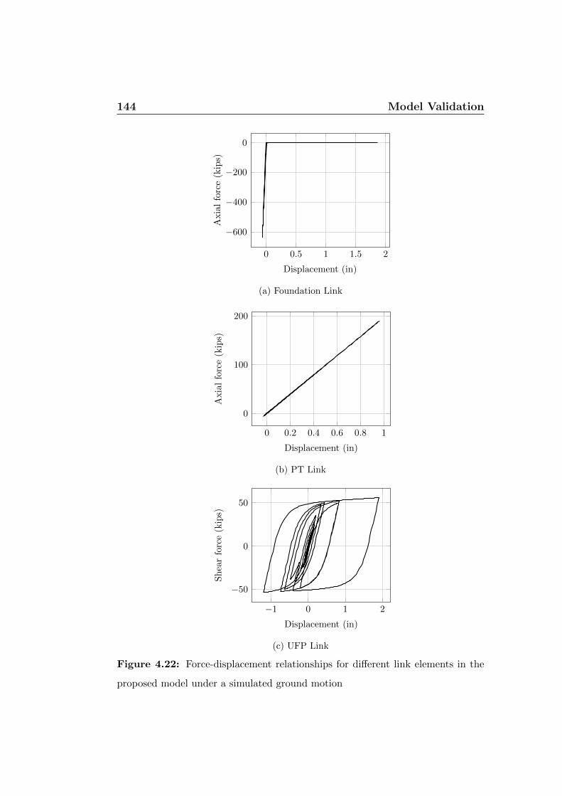
144 Model Validation
0 0.5 1 1.5 2
−600
−400
−200
0
Displacement (in)
Axia
lfo
rce
(kip
s)
(a) Foundation Link
0 0.2 0.4 0.6 0.8 1
0
100
200
Displacement (in)
Axia
lfo
rce
(kip
s)
(b) PT Link
−1 0 1 2
−50
0
50
Displacement (in)
Sh
ear
forc
e(k
ips)
(c) UFP Link
Figure 4.22: Force-displacement relationships for different link elements in the
proposed model under a simulated ground motion
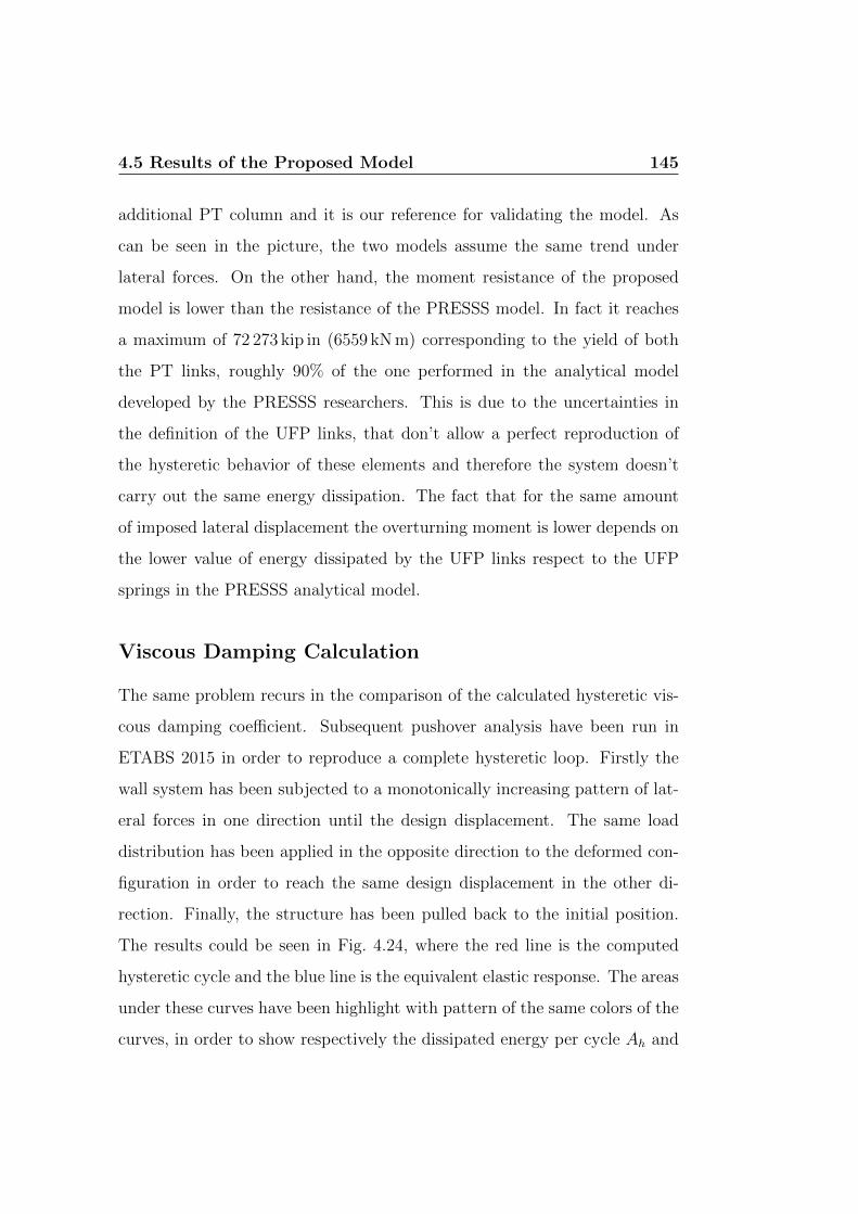
4.5 Results of the Proposed Model 145
additional PT column and it is our reference for validating the model. As
can be seen in the picture, the two models assume the same trend under
lateral forces. On the other hand, the moment resistance of the proposed
model is lower than the resistance of the PRESSS model. In fact it reaches
a maximum of 72 273 kip in (6559 kN m) corresponding to the yield of both
the PT links, roughly 90% of the one performed in the analytical model
developed by the PRESSS researchers. This is due to the uncertainties in
the definition of the UFP links, that don’t allow a perfect reproduction of
the hysteretic behavior of these elements and therefore the system doesn’t
carry out the same energy dissipation. The fact that for the same amount
of imposed lateral displacement the overturning moment is lower depends on
the lower value of energy dissipated by the UFP links respect to the UFP
springs in the PRESSS analytical model.
Viscous Damping Calculation
The same problem recurs in the comparison of the calculated hysteretic vis-
cous damping coefficient. Subsequent pushover analysis have been run in
ETABS 2015 in order to reproduce a complete hysteretic loop. Firstly the
wall system has been subjected to a monotonically increasing pattern of lat-
eral forces in one direction until the design displacement. The same load
distribution has been applied in the opposite direction to the deformed con-
figuration in order to reach the same design displacement in the other di-
rection. Finally, the structure has been pulled back to the initial position.
The results could be seen in Fig. 4.24, where the red line is the computed
hysteretic cycle and the blue line is the equivalent elastic response. The areas
under these curves have been highlight with pattern of the same colors of the
curves, in order to show respectively the dissipated energy per cycle Ah and

146 Model Validation
0 1 2 3 4 5 6 7 8 9 10 11 12 130
2
4
6
8·104
Top Displacement (in)
Bas
eM
omen
t(k
ip-i
n)
(a) Proposed Model pushover
(b) PRESSS pushover
Figure 4.23: Proposed Model Base moment-Top displacement relationship,
pushover results

4.5 Results of the Proposed Model 147
−8 −6 −4 −2 0 2 4 6 8
−250
−200
−150
−100
−50
0
50
100
150
200
250
Top Displacement (in)
Bas
eShea
r(k
ips)
Hysteretic loopElastic
Figure 4.24: Full cycle hysteresis loop
the equivalent elastic strain energy Ae, in according to Eq. (4.12).
The computed hysteretic viscous damping coefficient is equal to 15.24%,
that it is lower than the value presents in the PRESSS reports, that is 15.78%.
The result is a confirm of the consideration that the energy dissipated by the
UFP links in the proposed model is too small and not representative of the
real problem. Lacks in PRESSS reports about them don’t allow more accu-
rate definition of the nonlinear behavior of the shear connectors. However,
the resulting equivalent viscous damping coefficient remains coherent with
the value assumed in the design procedure.

148 Model Validation
Results of the Time Histories
The proposed model remains a good estimator of the global behavior of the
lateral load resisting system subject of study. Two design spectrum com-
patible ground motions, in particular the Loma Prieta earthquake and the
Northridge earthquake (Fig. 4.20), have been considered. Fig. 4.25 displays
the trend of the displacement in time of each floor level under these seismic
excitations during the first 20 seconds, when the ground accelerations are
more severe. It can be seen that the lateral displacement of the roof level
is lower than the one assumed for the design, relative to 2% drift limit. In
fact the maximum displacement during the Loma Prieta earthquake is 8.52 in
(216 mm) and during the Northridge earthquake is 8.84 in (225 mm), while
the design target displacement is 9 in (229 mm). Moreover, Fig. 4.26 shows
the full time history of the top displacement during the same ground motion.
When the earthquake finishes, the structure still has self-centering capacity.
So the wall comes back to its initial position and the residual displacement
is zero.
Finally, the base moment hysteresis loop during a simulate seismic exci-
tation is described by Fig. 4.27. The former is the cycle when the proposed
model is subject to the Loma Prieta ground motion while the second is the
nonlinear behavior under the Northridge time history. The figure shows
the self-centering characteristics of the split wall panel system by the “flag-
shaped” hysteresis loop, according to the theoretical considerations made in
Chapter 3.

4.5 Results of the Proposed Model 149
Figure 4.25: Floor Displacements time histories

150 Model Validation
0 5 10 15 20 25 30 35 40 45 50−8
−6
−4
−2
0
2
4
6
8
10
Time (s)
Dis
pla
cem
ent
(in)
(a) Loma Prieta Ground Motion
0 5 10 15 20 25 30 35 40 45 50−6
−4
−2
0
2
4
6
8
10
Time (s)
Dis
pla
cem
ent
(in)
(b) Northridge Ground Motion
Figure 4.26: Top Displacement time history

4.5 Results of the Proposed Model 151
−6 −4 −2 0 2 4 6 8
−8
−6
−4
−2
0
2
4
6
8
·104
Time (s)
Dis
pla
cem
ent
(in)
(a) Loma Prieta Ground Motion
−3 −2 −1 0 1 2 3 4 5 6 7 8 9
−0.6
−0.4
−0.2
0
0.2
0.4
0.6
0.8
1·105
Time (s)
Dis
pla
cem
ent
(in)
(b) Northridge Ground Motion
Figure 4.27: Base moment hysteresis loop

152 Model Validation

Chapter 5
Case Study: New Long Beach
Civic Center
5.1 Introduction
The objective of this chapter is the application of unbonded post-tensioned
hybrid walls as lateral resisting system of the New Long Beach Civic Center
(Long Beach, California). This building is considered an essential facilities
and therefore the owner required that it should guarantee enhanced levels
of seismic performance. In fact, it should experience of few or no injuries,
the new facility must be reoccupable within a week, full functionality should
be guaranteed within 30 days after a design earthquake and it results that
financial loss due to the design earthquake would be lower than 5 %. In order
to achieve the required seismic performance the use of enhanced walls has
been explored. As it has been presented previously, this kind of wall assured
a rocking behavior that results in small or zero residual displacement after
the design earthquake. Thus, this behavior concentrates all the non-linearity
at the base of the wall and guarantees that the remainder of the wall behaves

154 Case Study: New Long Beach Civic Center
almost linear elastic limiting damage. The self-centering behavior is provided
by unbonded post-tensioned tendons, but they have to be combined with an
energy dissipation system that softens the lateral displacements.
In Chapter 2, two different design procedures have been explored and the
lateral seismic forces applied to the structure have been computed. These
forces can be used to determine the material quantities required to provide
enough strength and a certain level of performance of the building, for ex-
ample in terms of drift of lateral displacement (see Chapter 3). Chapter 4
instead focuses on the development of a modeling procedure that could re-
produce the expected behavior of unbonded post-tensioned concrete hybrid
walls. The model variation exercise was necessary in order to verify the sec-
tional design developed thanks to the guidelines present in Chapter 3 on the
basis of the seismic forces computed according to Chapter 2.
In the following Chapter all these operations will be applied to an un-
bonded post-tensioned shear wall as part of the New Long Beach Civic Cen-
ter. In fact moving away from the feasibility design already made by the
engineers of Skidmore, Owings and Merrill LLP, new configurations have
been explored and a single shear wall with different design assumptions has
been studied. Initially, an unbonded post-tensioned hybrid shear wall has
been considered with mild reinforcement that provides the required energy
dissipation thanks to its elongation, while post-tensioned tendons running all
along the wall height give a restoring force that limits the lateral displace-
ment after the earthquake occurs. As requested by the client, the considered
structure is cast-in-place and not precast as the PRESSS test building, but
this difference does not imply changes in the design of the wall base, which is
the more critical part for this kind of structure. Moreover, the same proce-
dure has been applied to a conventional monolithic reinforced concrete shear

5.2 New Long Beach Civic Center 155
wall in order to compare the results between these two options.
5.2 New Long Beach Civic Center
The case study considered is the New Long Beach Civic Center (Long Beach,
California). Fig. 5.1 shows the site plan of the whole project of renovation of
the downtown of Long Beach. The project includes a new City Hall, a new
Port Building for Harbor Department administration, a new and relocated
Main Library, a redeveloped Lincoln Park, a residential development, and a
commercial mixed use development. In total, the proposal includes six new
buildings, three new parking garages, related infrastructure and landscaping,
and two new public street extensions through the project site. Both the City
Hall and Port buildings would be up to 11 stories in height.
Skidmore, Owings and Merrill LLP (SOM) has been involved in the design
of Civic Center Block, that includes the City Hall and the Port Administra-
tion Building (Fig. 5.2). The former would be an approximately 270 000 gross
square feet (gsf) (25 084 m2) up to 11-story concrete frame structure that in-
cludes office space for City staff and elected officials. The structure would also
include Council Chambers, meeting rooms, transaction counters and other
public serving components. The Port Building would be up to 11 stories,
utilizing a concrete frame structure of up to 240 000 gsf (22 300 m2). It would
be designed to house the administrative functions of the Harbor Depart-
ment. The space within this building would be primarily office space. City
Hall Building. Located around and between the City Hall and Port Building
would be a 73 000 square foot (sf) (6782 m2) Civic Plaza, which would include
landscape elements appropriate for larger spontaneous gatherings as well as
planned events. The Port and City Hall buildings would share a common

156 Case Study: New Long Beach Civic Center
Figure 5.1: Global view of Civic Center
underground parking structure that includes shared infrastructure such as
the combined central plant, common points of vehicular access and shared
loading dock services.
Fig 5.3 shows the typical elevation of the building. The City Hall and the
Port Building present an equal building layout, with a total height of 162.5 ft
(49.53 m) above ground, while the levels below ground are in common. Also
the plan of the two building is identical and the typical framing is shown in
Fig. 5.4. The lateral resisting system of these building is composed by two
concrete cores placed symmetrically with respect to the central axis. These

5.2 New Long Beach Civic Center 157
two cores contain stairs and elevators. The frame system has a typical bay
of 30 ft (9.14 m) in one direction and is designed to carry only the gravity
loads, with no contribution in the seismic resistance.
Figure 5.2: Global view of Civic Center
Long Beach is located in a region with high seismicity. The owner requires
not only the collapse of the structure during an earthquake be prevented, but
also that the structure be costly efficient as well, in terms of structural and
non-structural repair and in terms of loss of business operation after the
seismic event. Therefore, the design requirement for the Civic Center is that
it should have a 50% confidence level that after the design earthquake occurs,
the Civic Center should be able to:
• Experience few or no injuries;
• Reoccupation of the new facility within a week;

158 Case Study: New Long Beach Civic Center
Figure 5.3: Typical system elevation
Figure 5.4: Typical tower framing plan

5.2 New Long Beach Civic Center 159
• Recover full functionality within 30 days;
• Experience less than 5% financial loss (as compared to the replacement
value).
In order to achieve this very strict performance level superstructure and
foundations have to remain remain essentially elastic during the seismic
event. Moreover the relative displacements should be very low in order to
limit damage of non-structural components, which however need to be de-
signed to accommodate relative displacements. Mechanical, electrical and
plumbing components and other critical systems need to be protected to
make sure that they are replaced/repaired within 1 month after the earth-
quake. This enables normal operations to resume once utilities are restored.
Following the American building code, these considerations mean that the
Civic Center falls into the Risk Category IV (Table 1.5-1, ASCE 7-10), which
implied a drift limit of 1% (Table 12.12-1, ASCE 7-10).
Enhanced walls that perform an almost elastic behavior are needed. In
order to know the behavior of the whole structure using this kind of walls
and their advantages, previously it is necessary to study the behavior of a
single wall. For this reason, the present research takes into consideration one
wall which runs parallel to the shorter side of the building. The interaction
with the other walls composing the lateral resisting system could be a future
development of this work. In order to limit the coupling between walls placed
orthogonally, the plan layout has been changed, as shown in Fig. 5.5, where
the red boxes are the proposed location of the walls. This is possible because
the building plan is not definitive yet, giving the possibility to suggest new
configurations. It is obvious that the location of the walls must be confirmed
by the architects, but it is not relevant in the present research.
An independent engineering consultant carried out a geotechnical investi-

160 Case Study: New Long Beach Civic Center
Figure
5.5:
Prop
osedp
lan

5.2 New Long Beach Civic Center 161
0 1 2 3 4 5 6 70
0.2
0.4
0.6
0.8
1
1.2
1.4
Period (s)
Sa
(g)
Figure 5.6: Site-Specific Response Spectrum
gation and one of the objectives was proposing a site-specific response spec-
trum for a better evaluation of the possible earthquake-induced loads which
may be experienced by the considered building during its design life. There-
fore, they have performed a Probabilistic Seismic Hazard Analyses (PSHA)
and a Deterministic Seismic Hazard Analyses (DSHA) using the computer
program EZ-FRISK (Risk Engineering, 2014) in order to develop site-specific
response spectra in accordance with 2013 CBC and Chapter 21 of ASCE 7-
10. In Fig. 5.6, it is possible to see the site-specific response spectrum used
in the following analysis.
Finally, the following uniformly distributed loads have been considered
at each level. The self-weight of the members is not listed because it is
automatically computed by the software.

162 Case Study: New Long Beach Civic Center
Table 5.1: Uniformly Distributed Loads
Load Name Load TypeValue
USCS SI
Live Load
Typical Level LL 100 psf 4.8 kPa
Roof Level LL 150 psf 7.2 kPa
Partition 10 psf 0.48 kPa
Superimpose Dead LoadTypical Level SDL 35 psf 1.7 kPa
Roof Level SDL 40 psf 1.9 kPa
5.3 Wall Description
The considered wall runs parallel to the shorter side of the building (see
Fig 5.5). Since they are placed in a symmetric fashion and the torsional
effects are not considered in the present research, they are subjected to the
same actions during a seismic event. The wall is 162.5 ft (49.53 m) tall and
37.5 ft (11.43 m) wide. The effective seismic mass corresponds to half of the
mass of the building, since in that direction the lateral resistance is provided
by 2 wall placed symmetrically in plan. The gravity mass supported by
the considered wall corresponds to the sum of the weight of each floor level
corresponds to its tributary area. Thus, the effective seismic mass at each
floor level is the 50% of the total floor mass, while the tributary weight is
the 7.4% of it. As already said, the structural typology taken into account is
an unbonded post-tensioned concrete hybrid wall, whose material properties
are listed in Table 5.2.
The energy dissipation system combined with the wall system is com-
posed by mild reinforcement placed at the interface between the wall and
the foundation and debonded for a certain length inside the concrete.

5.4 Design Procedure 163
Table 5.2: Material Properties
Material Properties SymbolValue
USCS SI
Steel
Nominal yield strength fy 60 ksi 414 MPa
Failure strength fus 90 ksi 621 MPa
Modulus of elasticity Es 30458 ksi 210 GPa
Concrete Nominal strength f ′c 6 ksi 41.4 MPa
Tendon
Tensile strength fupt 270 ksi 1861.6 MPa
Yield strength fypt 245 ksi 1689 MPa
Tendon diameter d 0.5 in 13 mm
Tendon area A 0.153 in2 98.7 mm2
Modulus of elasticity Ep 28500 ksi 196.5 GPa
Initial prestress fse 149.2 ksi 1028.5 MPa
5.4 Design Procedure
The wall has been designed with both the FBD and DDBD method. The
two procedure applied to the wall are presented in the following sections.
5.4.1 Direct Displacement-Based Design
The design procedure computed with the DDBD takes into account the actual
behavior of the structure. Once the design drift is set, the displacement
profile along the wall follows its deformed shape. In the case study the wall
behaves like a rigid block and it has to remain essentially elastic. For this
reason, the profile displacement results to be linear along the height of the
wall. The yield displacement reflects the high level of ductility provided by
the wall that is also takes into account in the equivalent viscous damping
defined for the specific hysteretic rule of the system.

164 Case Study: New Long Beach Civic Center
Table 5.3: Design displacement at each level
LevelHeight Wall Displacement
USCS SI USCS SI
Top 162.5 ft 49.5 m 1.625 ft 0.495 m
Roof 158.0 ft 48.2 m 1.580 ft 0.482 m
11 142.0 ft 43.3 m 1.420 ft 0.433 m
10 129.0 ft 39.3 m 1.290 ft 0.393 m
9 116.0 ft 35.4 m 1.160 ft 0.354 m
8 103.0 ft 31.4 m 1.030 ft 0.314 m
7 90.0 ft 27.4 m 0.900 ft 0.274 m
6 77.0 ft 23.5 m 0.770 ft 0.235 m
5 64.0 ft 19.5 m 0.640 ft 0.195 m
4 51.0 ft 15.5 m 0.510 ft 0.155 m
3 38.0 ft 11.6 m 0.380 ft 0.116 m
1 0.0 ft 0.0 m 0.000 ft 0.000 m
Design Criteria Wall with unbonded prestressing will rarely be governed
by strain limitations and thus the critical value is the drift at the top floor.
θc = 0.01 (5.1)
Design Displacement Since the design deformation is dominated by sin-
gle crack at the base of the wall, the design displacement profile may be
assumed to be linear along the height and it is defined through the 1% drift
multiplied by the progressive height hi corresponding to the height of each
story level of the Civic Center.
∆i = θchi (5.2)
The values are shown it Table 5.3.
Hence the design displacement results to be:
∆d =
∑ni=1(mi∆
2i )∑n
i=1(mi∆i)= 1.115 ft(0.400 m) (5.3)

5.5 Wall Description 165
Yield Displacement The yield drift depends on the material sizes and
structural geometry defined for the wall in
5.5 Wall Description
. It can be based on the stiffness of the uncracked wall section up the full
height. For reinforced cantilever wall buildings, the maximum drift occurs
at the top of the building and the yield drift can be defined through the
following dimensionless yield curvature:
lwφy = 2.00εy (5.4)
Assuming a linear distribution of curvature over the height, with hn =
162.5 ft(49.53 m) and lw = 37.5 ft(11.43 m), the yield drift at roof level results
to be:
θyn = εyhn/lw = 0.0085 (5.5)
Due to the high level of ductility provided by the system with mild re-
inforcement, the yield displacement of a prestressed wall can be assumed to
be approximately of 40% of the one of a reinforced concrete wall. Hence, it
results to be:
θy = 0.4εyhn/lw = 0.0034 (5.6)
Displacement Ductility Since the design displacement profile is almost
linear, the displacement ductility can be approximated by:
µ = θc/θy = 2.929 (5.7)
Effective Mass The effective mass of the SDOF structure results from
the consideration of the masses mi computed at each floor level of the Civic

166 Case Study: New Long Beach Civic Center
Center:
me =n∑i=1
mi∆i
∆d
= 21.95 kip s2/in(3843.2 ton) (5.8)
Equivalent Viscous Damping The effective damping depends on the
structural system and on the displacement ductility µ. As already said in
Chapter 3, one of the key aspect for an efficient design of an hybrid wall is the
proportioning between the yielding contribution, which is responsible for the
energy dissipation of the system, and the self-centering contribution. This
design criteria could be summarized as the ratio κd between the yielding
components and the elastic restoring components. The value of this ratio
determines the amount of dissipated energy and the re-centering ability of
the system.
The nominal base moment strength of an unbonded post-tensioned hy-
brid wall can be seen as the sum of three components, Mwn, Ms and Mpt,
representing respectively the contributions of applied axial loads, the wall
mild steel reinforcement and PT tendons. Thus the parameter κd, proposed
by Kurama and called “ED steel moment ratio” is defined as:
κd =Ms
Mpt +Mwn
(5.9)
An appropriate value for κd should be selected for design. If the yielding
contribution is too small (i.e., κd ratio is too small), then the system doesn’t
provide adequate energy dissipation. Conversely the self-centering capability
of the wall may be too small and thus it may not be sufficient to close the
gap opening at the base joints after the seismic event, if the κd ratio is too
large. The values proposed for this parameter range from 0.50 to 0.80 to
satisfy the required performances. The value selected in the present case is
κd = 0.75.

5.5 Wall Description 167
The effective damping can be computed through the equation proposed
by Priestley [16] for flag-shaped hysteresis, that for a generic value of κd and
r (post-yield stiffness ratio) is given by:
ξarea =Ehysteresis
4πEelastic
=κd(µ− 1)
µπ(1 + r(µ− 1))(5.10)
In Eq. 5.10 Ehysteresis represents the energy dissipated and Eelastic repre-
sents the energy that would be stored in an equivalent purely elastic system
without dissipation. These two quantities are represented in Fig. 5.7 respec-
tively by the blue area and the red one.
Figure 5.7: Idealized hysteretic damping calculation
The damping calculated from Eq. 5.10 has to be multiplied by the cor-
rection factor from Fig. 5.8 and has to be added to the elastic damping com-
ponent. The estimate of EVD is established in [16] for hysteresis rules with
specific characteristics. When the hysteresis rules have different character-
istics than those presented by Priestley, the appropriate ductility/damping
equations defined with inelastic time-history analysis (ITHA) have to be

168 Case Study: New Long Beach Civic Center
Figure 5.8: Correction factors to be applied to the area-based equivalent viscous
damping ratio, Priestley [16]
developed. Some correct estimates of the relationship can be obtained by
comparing the relationship between the area-based viscous damping, given
by Eq. 5.10 which can be computed for any system if the hysteretic compo-
nent is known, with the hysteretic component of viscous damping calculated
for specific level of displacement ductility. This relationship is plotted in
Fig. 5.8 for six hysteretic rules that are: elastic-perfectly plastic (EPP), bi-
linear (BI), Taketa Thin (TT), Taketa Fat (TF), Flag with κd = 0.35 (FS)
and Romberg-Osgood (RO).
The vertical axis is the ratio between the hysteretic component of the
equivalent viscous damping computed from ITHA and the area-based one
found from Eq. 5.10. This can be considered as an appropriate correction
factor to be applied to the area-based viscous damping and it can be com-
puted with Fig. 5.8 for a known level of displacement ductility. The three

5.5 Wall Description 169
data point are defined for each hysteresis rule for ductility levels of 2, 4 and
6. This approach represents a suitable alternative to estimate time-history
analysis. In the present case the area-based EVD is ξarea = 15.1% and the
displacement ductility is µ = 2.929. Hence, this results in a correction factor
R = 0.65.
Finally the elastic damping is estimated to be ξel = 0.05 and thus the
equivalent viscous damping results to be:
ξeq = ξel +Rξarea = 14.84% (5.11)
Design Displacement Spectra The design displacement spectrum is de-
fined for the evaluated level of equivalent viscous damping. The displace-
ment spectrum can be considered to be independent from the period after
the corner period that can be evaluated from the moment magnitude. In the
present case the corner period is computed to be Tc = 4 sec. The relative
design displacement spectrum can be developed from the acceleration spec-
trum for 5 percent damping. Initially the elastic displacement spectrum is
calculated and then it will be modified for the correct value of damping. The
displacement spectrum for 5% of damping can be defined as:
∆(T,5) = S(T,5) g T2/(4π2) (5.12)
The displacement spectra for the present level of ξeq results from:
∆(T,ξeq) = ∆(T,5) ·(
0.07
0.02 + ξ
)0.5
(5.13)
Both of them are represented in the graph in Fig. 5.9.
The design displacement spectrum at Tc results to be ∆(Tc,ξ) = 15.2 in (0.386 m).

170 Case Study: New Long Beach Civic Center
0 1 2 3 4 50
0.1
0.2
0.3
0.4
0.5
Period (s)
Dis
pla
cem
ent
Sp
ectr
a(m
)
ξel
ξeq
Figure 5.9: Response displacement spectra
Effective Period The effective period corresponding to the design dis-
placement can be found by proportion as:
Te = Tc ·∆d
∆(Tc,ξ)
= 3.52 sec (5.14)
Effective Stiffness The effective stiffness can be found by the effective
mass and the effective period and it results to be:
Ke =4π2me
T 2e
= 69.97 kip/in (12 254 kN/m) (5.15)
Design Base Shear The design shear at the base of the wall is defined
through the design displacement and the effective stiffness. It is equal to:
F = Vbase = Ke ∆d = 936 kips (4164 kN) (5.16)
Moment Base Design The evaluated base shear must be distributed as
design force to the different lumped masses of the wall in proportion to their

5.5 Wall Description 171
value and displacement. In this way the design moments at plastic hinges
location can be established. The design force at level i results to be:
Fi = Vbase ·mi∆i∑n
j=1(mj∆j)(5.17)
The design moment at the base of the wall resulting from this distribution
of forces is Mbase = 104.362 kip ft(141 496 kN m).
5.5.1 FBD Comparison
The design procedure for the unbonded post-tensioned hybrid wall has been
computed also with the Force-Based Design method. The values considered
a reduction factor R = 5, the deflector amplification factor Cd = 5 and
importance factor I = 1, according to ASCE 7-10 standard. The forces
resulting from FBD procedure are:
Vwd = 1939.4 kips (8627 kN)
Mwd = 215 833 kips ft (305 424 kN m)
Nwd = 2179 kips (9694.4 kN)
These forces result to be much higher than those found with the DDBD
method, except for the axial force that results from the tributary area of the
considered wall and therefore it remains the same. In particular the base
shear is around 50% higher than the one resulting from the DDBD method-
ology. This overestimation is compatible with the results of the PRESSS
program, as shown in the previous Chapter. However, the analytical model
of the wall designed with the forces of the DDBD method behave well, as
proved through pushover analysis and inelastic time-history analysis pro-
posed later. It is possible to see that the discrepancy between the methods
results in a substantial increasing of required material.

172 Case Study: New Long Beach Civic Center
5.6 Base Cross-Section Design
The design forces are the design shear Vwd = 936 kips (4164 kN), the design
moment Mwd = 104.362 kip ft(141 496 kN m) both defined in the previous
section, and the value of gravity load defined through the tributary area
of the wall. The value of gravity force is Nwd = 2179.4 kips (9694.4 kN).
Once the design forces are know, the base cross-section can be designed
establishing the required material quantities. This implies the definition of
the amount of PT steel and ED steel, their location and the wall dimensions
necessary to satisfy the wall design base forces. The wall section should have
a symmetric layout and the ED and PT steel should be placed outside the
confined regions at the wall toes. The analytical design procedure has been
presented in Chapter 3. In this section its main aspects will be presented in
order to compute the resulting material quantities.
Section Layout and Initial Assumptions The PT tendons will be placed
less eccentric than the ED bars in order to have higher deformation in the
mild reinforcement than in the tendons. In the computations, the steel
areas are considered lumped in two areas placed symmetrically respect to
the centerline. The eccentricity of the PT tendons from the wall center-
line is assumed to be ep = 3.28 ft (1.00 m) and the one of the ED steel of
ep = 6.56 ft (2.00 m). Moreover, the initial assumption of the wall thickness
is tw = 16 in (0.41 m). The unbonded length of the PT tendons is equal to
the wall height in order to distribute the strains and keep the tendons in the
elastic field.

5.6 Base Cross-Section Design 173
Steel Quantities Since lumped steel areas are considered in the present
case, the governing equilibrium equations at the base cross section are:
Cd = 0.85 f ′c tw β1 xn (5.18)
Cd = Nwd + 2Asσs,m + 2Aptσpt,m (5.19)
Mwd
φf= Cd
(lw2− β1
xn2
)(5.20)
The design is made without iterations and the neutral axis xn is solved
directly from Eqs. (5.18) and (5.20). The steel areas are computed using
Eqs. (5.19) and (5.9), after the definition of their relative strains and stresses.
From the value of the neutral axis length the ED steel and PT steel elon-
gations can be computed using the displaced configuration and the selected
location of the bars (es) and tendons (ep) from the wall centerline. The deter-
mination of these elongations is not based on compatibility but on kinematic.
In fact when the gap opens at the base, the PT steel and the ED steel are
debonded to the concrete and therefore the hypothesis of perfect adherence
between steel and concrete is no more valid. It is necessary to use kinematic
considerations due to base section rotation, that creates an elongation of
the debonded mild reinforcement and of the unbonded PT steel. Then the
stresses σs,l, σs,r and σpt,m are calculated with the selected unbonded length
(ls and lpt) and the selected stress-strain relationship. The required Apt and
As can be found by solving Eqs. (5.19) and (5.9) for the assigned value of
κd. In the present research the stresses of the ED steel lumped areas have
been assumed equal to the yield stress fy and the bedonding length is then
calculated as the minimum length that assure the yield elongation in the ED
steel for the calculated neutral axis.
The resulting neutral axis and ls will be:
xn = 10.9 ft (3.334 m)

174 Case Study: New Long Beach Civic Center
ls = 7.5 ft (2.275 m)
The required value of Apt and the respective number of tendons npt at each
side results to be:
Apt = 7.19 in2(4639 mm2)
npt = 47
The required value of As and the respective number of rebar ns (#10 accord-
ing to American standards, corresponding to a nominal diameter of 1.27 in,
so 32.3 mm) at each side result to be:
As = 29.21 in2(18 845 mm2)
ns = 23 #10
Design Check Part of the design objectives is that, under the design level
of ground motion, the PT steel remains in the linear-elastic range and that
the ED steel yields during the seismic event. It is possible to verify these
requirements computing the elongation and the stress level in the steel. Re-
garding the PT tendons, the strain and stress level has to be lower than the
yielding one. On the other hand, it has to be proved that the strain and
stress in the ED steel are higher than the yielding level.
In the present work the respective values of stress and strain for the two
materials have been computed for their established length of debonding. It
has been verified that their values respect the required limits.
An other objective is to assure that shear slip at the base horizontal joint
does not occur. It is considered to be satisfied for the design earthquake
but it has to be verified for the maximum considered earthquake, that is not
take into consideration the present work. For this check and for the other
requirement necessary to satisfy the design goals it is possible to refer to

5.7 Analytical Validation of the DDBD procedure 175
Kurama’s prescriptions [23]. Also the design of the confinement of the base
cross-section can be determined referring to [23]. The confinement of the
wall base is fundamental in order to have the non-linearity primarily dues to
gap opening at the base and in the concrete in compression only at the wall
toes.
Moreover, the direct displacement-based design method requires that the
estimated hysteretic damping (computed with Eq. (5.11)) has to be compared
with the energy dissipated by the structure per load cycle. It will be discussed
later, in Sec.5.7.
5.7 Analytical Validation of the DDBD pro-
cedure
Once the design of the lateral load resisting system has been performed,
the results must be validated. Since there is not the possibility to create a
test building in order to simulate the response of the designed wall under
a ground motion, an analytical model has been developed. The unbonded
post-tensioned hybrid concrete wall is modeled following the procedure de-
veloped at Chapter 4. The only difference with the jointed walls is the
energy dissipation device, here obtained thanks to mild reinforcement which
is debonded at the base in order to allows its yielding when the earthquake
occurs. In the present research the ED steel has been modeled is a similar
way as the post-tensioned tendons. In fact the relative lumped areas used in
the design have been modeled as link elements at the base of the wall and
placed in the actual location of the designed base section. With respect to
the u-shaped flexural plates, the present energy dissipation device has a well
known hysteretic function and its nonlinear behavior could be assumed as

176 Case Study: New Long Beach Civic Center
Figure 5.10: Wall base layout of the model of a hybrid wall
elastic-perfectly plastic. In a similar way of what did for the PT links, the
stiffness of the ED links is:
kED =EsAsls
(5.21)
where Es is the modulus of elasticity of the mild steel, As is the lumped areas
of the link under consideration and ls is its debonded length.
The yielding force Fy,ED is calculated as the product of the yield stress
fs and the ED steel area As.
See Fig. 5.10 for the base layout of the unbonded post-tensioned hybrid
wall developed in ETABS 2015.
The characteristics of all the elements that compose the analytical model
are summarized in Table 5.4. Their definition follows the modeling assump-
tions developed in Chapter 4. The stiffness of the foundation links is 10
times higher that the one proposed in the PRESSS research program. This

5.7 Analytical Validation of the DDBD procedure 177
Table 5.4: ETABS Model - Properties of the Components
Component PropertyValue
USCS SI
Wall MemberElastic Mod. Ec 3605 ksi 24.855 GPa
center of compr. 48.23 in 1.225 m
Found. Links
Stiffness kFL 100 000 kip/in 17 512 684 kN/m
Yield Force Fy,fl C 10 000 kips 44 482 kN
Yield Force Fy,fl T 0.1 kips 0.45 kN
PT Links
Stiffness kPT 2828.1 kip/in 15 393.5 kN/m
Post-Yield Ratio 0.02 0.02
Yield Force Fy,pt T 576.91 kips 2566.24 kN
Yield Force Fy,ptC 2371.23 kips 10 547.76 kN
ED LinksStiffness kED 381 708 kip/in 2 077 679 kN/m
Yield Force Fy,ED 1564.25 kips 6958.15 kN
value has been decided in order to minimize the initial shortening of the links
due to the prestressing force. A better evaluation should be preferred in a
further study and its influence in the global response of the structure could
be part of a future development of the present research. The yielding force
in compression of these links has been calibrated in order that they remain
in the elastic range when the design top displacement is applied to the wall
system.
As for the masses, the forces applied to the structure when the design
earthquake occurs, the vertical loads are modeled as concentrated forces ap-
plied on the foundation links. They are symmetric and worth 1987 kips
(8838 kN), calculated as half of the sum of the initial prestress equal to
1794 kips (7982 kN) and the axial force acting on the wall, equal to 2178 kips
(9694 kN). Effective seismic mass at each level instead is modeled as lumped
masses at the centerline of the wall and they work only in the horizontal
direction and not in the vertical one. The nodes in correspondence with the

178 Case Study: New Long Beach Civic Center
0 0.5 1 1.5 2 2.5 3 3.5 40
0.2
0.4
0.6
0.8
1
1.2
1.4
1.6
Period (s)
Sa
(g)
Site-SpecificFriuli
Loma Prieta
Figure 5.11: Response spectra comparison
foundation link on the right of the wall is laterally fixed, in order to avoid
shear slip.
Regarding the dynamic nonlinear analysis, Seismomatch software has
been used in order to determine ground motions that are compatible with the
site-specific response spectrum, as in Chapter 4. The 2 accelerograms that
better converge are the Friuli (1976)record and the Loma Prieta, California
(1989) record. Their spectrum compatible ground motions are presented in
Fig. 5.12, while Fig. 5.11 shows their matched response spectra in comparison
with the target one.

5.7 Analytical Validation of the DDBD procedure 179
Figure 5.12: Case study, response spectrum compatible time histories

180 Case Study: New Long Beach Civic Center
5.7.1 Damping Validation
The hysteretic damping calculated during the DDBD procedure has to be
compared with the energy dissipated by the structure per load cycle. The
energy dissipated by the lateral resisting system under lateral loads can be
determined with a cyclic pushover analysis. As in Chapter 4, the 3 subsequent
nonlinear static analysis have been run controlling the top displacement:
firstly till the design displacement, then back till the design displacement
in the opposite direction and finally to the initial undeformed configuration.
Fig. 5.13 shows on blue the result of the cyclic pushover analysis, highlighting
also the area enclosed by the curve, which describes the energy dissipated by
the structure. The green area instead represents the equivalent elastic strain
energy. From the graph it results ξhyst = 14.76%, that summed with the 5%
elastic damping consists in an equivalent viscous damping much higher that
the 14.84% theoretically computed.
−20 −10 0 10 20
−1,000
−500
0
500
1,000
Top Displacement (in)
Base
Sh
ear
(kip
s)
Hysteretic loop
Elastic
Figure 5.13: Case study, full cycle hysteresis loop, first iteration

5.7 Analytical Validation of the DDBD procedure 181
Further iterations are therefore required. The computed hysteretic damp-
ing is used for the calculation of the forces acting on the unbonded post-
tensioned hybrid wall and so in the definition of the material quantities,
following all the steps presented in the previous sections. This procedure
must be repeat till convergence of the hysteretic viscous damping. The final
quantities are listed below, corresponding to an hysteretic damping coeffi-
cient of 12.9%. The concentrated vertical load at the center of compressions
is equal to 1934 kips (8603.6 kN).
The base design forces are:
Base Shear Vwd: 861 kips (3829 kN)
Base Moment Mwd: 1 103 490 kip in (130 129 kN m)
Base Axial Load Nwd: 2179.4 kips (9694.4 kN)
Table 5.5: Material Quantities
USCS SI
PT TendonsApt 5.66 in2 3652 mm2
npt 37 37
ED Steel
As 26 in2 16 774 mm2
ns 20 #10 20 #10
ls 13.25 ft 4.04 m
Using those parameters of the single components in the analytical model,
the computed hysteretic viscous damping is 12.45%, coherent with the 12.7%
used for the design. Fig. 5.14 shows the relative hysteretic loop. Prediction
results described in subsequent sections have been obtained from the analyt-
ical model with the quantities presented above. In Fig. 5.14 it is possible to
see the perfect flag-shaped hysteretic loop of the designed unbonded post-
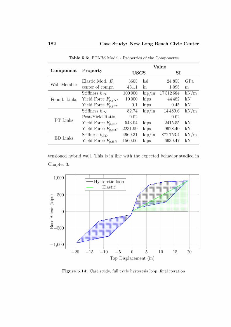
182 Case Study: New Long Beach Civic Center
Table 5.6: ETABS Model - Properties of the Components
Component PropertyValue
USCS SI
Wall MemberElastic Mod. Ec 3605 ksi 24.855 GPa
center of compr. 43.11 in 1.095 m
Found. Links
Stiffness kFL 100 000 kip/in 17 512 684 kN/m
Yield Force Fy,fl C 10 000 kips 44 482 kN
Yield Force Fy,fl T 0.1 kips 0.45 kN
PT Links
Stiffness kPT 82.74 kip/in 14 489.6 kN/m
Post-Yield Ratio 0.02 0.02
Yield Force Fy,pt T 543.04 kips 2415.55 kN
Yield Force Fy,ptC 2231.99 kips 9928.40 kN
ED LinksStiffness kED 4969.31 kip/in 872 753.4 kN/m
Yield Force Fy,ED 1560.06 kips 6939.47 kN
tensioned hybrid wall. This is in line with the expected behavior studied in
Chapter 3.
−20 −15 −10 −5 0 5 10 15 20
−1,000
−500
0
500
1,000
Top Displacement (in)
Bas
eShea
r(k
ips)
Hysteretic loopElastic
Figure 5.14: Case study, full cycle hysteresis loop, final iteration

5.7 Analytical Validation of the DDBD procedure 183
5.7.2 Pushover Results
A nonlinear static analysis was carried out in order to show the expected
structural behavior of the proposed unbonded post-tensioned hybrid wall
under lateral loads. It has been performed controlling the displacement of the
top level and considering an inverse triangular distribution of lateral forces
over the height of the wall. It is coherent with the DDBD design procedure,
that admits a linear profile of the wall displacements. The resulting base
moment-top displacement relationship in shown in Fig. 5.15. The change in
the structure stiffness here is more pronounced than seen for the PRESSS
test building. This is due to the different hysteretic behavior of the energy
dissipation device, here presented by mild steel that has been modeled with
a sharp discontinuity in the stress-strain response. So at the first point the
wall starts uplift, while the second and third points concern the first yield
of the ED links, the left and the right one respectively. The PT tendons
are not expected to yield within the 30 inches displacement limit considered
in the graph, assuring an elastic behavior in the practical applications and
therefore providing re-centering capability to the structure.
5.7.3 Results From Time Histories Analysis
Time histories analysis has been run in order to see the dynamic behavior of
the lateral resisting system considered during a simulated earthquake. Friuli
and Loma Prieta records has been used, as previously described. Fig. 5.16
shows the first 25 seconds of the behavior in time of the wall in terms of floor
displacement. Level 3, 6 10 and the top level have been considered. The max-
imum displacement during the Loma Prieta earthquake is 16 in (407 mm) and
during the Friuli earthquake is 13.62 in (346 mm). The target displacement

184 Case Study: New Long Beach Civic Center
0 2 4 6 8 10 12 14 16 18 20 22 24 26 28 300
0.2
0.4
0.6
0.8
1
1.2·105
Top Displacement (in)
Bas
eM
omen
t(k
ip-i
n)
Figure 5.15: Case study, Base moment-Top displacement relationship, pushover
results
considered in the design was 19.49 in (495 mm), so the predicted response is
lower than the target one. Moreover, the force-displacement relationships of
the different links show that the PT links remain in the elastic range and
the ED links yield, providing self-centering capacity and energy dissipation,
respectively. Fig. 5.17 shows the nonlinear response of those components
under the Loma Prieta ground acceleration, together with the response of
the foundation links, which work only in compression.
Finally, the time histories analysis show that the lateral resisting system
comes back to the undeformed configuration after the earthquake occurs.
In fact after 60 sec the horizontal displacement of the roof level is around

5.7 Analytical Validation of the DDBD procedure 185
0.118 in (3 mm) during the Loma Prieta ground motion and 0.079 in (2 mm)
during the Friuli ground motion.

186 Case Study: New Long Beach Civic Center
Figure 5.16: Floor Displacements time histories

5.7 Analytical Validation of the DDBD procedure 187
0 0.5 1 1.5 2 2.5
−5,000
0
Displacement (in)
Axia
lfo
rce
(kip
s)
(a) Foundation Link
0 0.5 1
0
50
100
Displacement (in)
Axia
lfo
rce
(kip
s)
(b) PT Link
0 0.5 1
−1,000
0
1,000
Displacement (in)
Sh
ear
forc
e(k
ips)
(c) ED Link
Figure 5.17: Force-displacement relationships for different link elements under
the Loma Prieta ground acceleration

188 Case Study: New Long Beach Civic Center
5.8 Comparison with a Conventional Rein-
forced Concrete Wall
The design procedure has been performed for the case of a conventional
concrete wall too. The forces found from the DDBD and FBD methods
were used to design the monolithic wall, which was then validated through
inelastic time-history analysis. The purpose of this exercise is to highlight
the advantages that come from the use of an unbonded post-tensioned hybrid
wall. Moreover, the application of the DDBD procedure to a well known
structure allows us to better understand the method and validate what it
has been done for a particular lateral resisting system.
The geometrical dimensions of the wall are the same considered previously
as well as the seismic mass and gravity loads, except for the wall thickness,
that must be to increased to 26 in (660 mm), in order to provide the required
strength. Concerning the material properties, for a cantilever concrete wall
the material strengths considered are the expected one. This is due to the fact
that the method considers the expected behavior of the wall identifying the
location of predicted plastic hinge at the base. Since the material strength
normally considered in the computations represents a conservative estimate,
in the case that the strength exceeds the design values, the resisting moment
developed at the plastic hinge will be greater than the design value. For
this reason it is recommended to use the expected strength rather than the
nominal one.
For a cantilever concrete wall the DDBD method considers the expected
behavior of the wall identifying at the base the location of a predicted plastic
hinge. The material strength normally considered in the computations repre-
sents a conservative estimate, so if the real strength exceeds the nominal one,

5.8 Comparison with a Conventional Reinforced Concrete Wall189
Table 5.7: Material Properties for a Cantilever Concrete Wall
Material Properties SymbolValue
USCS SI
Steel
Nominal yield strength fy 60 ksi 414 MPa
Expected yield strength 1.1 fy 66 ksi 455 MPa
Failure strength fus 90 ksi 621 MPa
Modulus of elasticity Es 30458 ksi 210 GPa
ConcreteNominal strength f ′c 6 ksi 41.4 MPa
Nominal strength 1.3f ′c 7.8 ksi 53.8 MPa
the resisting moment developed at the plastic hinge location will be greater
than the design value. This means that maybe the plastic hinge does not
occur in the predicted location, but somewhere else that was not designed for
that. For this reason it is recommended to use the expected strength rather
than the nominal one in the DDBD method. The material properties taken
into consideration are listed in Table. 5.7.
5.8.1 DDBD Procedure
The DDBD procedure for a conventional reinforced concrete wall is presented
below, following what already presented in Chapter 2.
Design Criteria The critical parameters for monolithic concrete walls re-
mains the drift at the top level. Thus the design drift is defined according to
ASCE 7-10, thus:
θc = 0.01 (5.22)
Design Displacement The design displacement profile follows the de-
formed shape of the wall. Since the design in governed by the code drift

190 Case Study: New Long Beach Civic Center
Table 5.8: Wall Displacement for a Cantilever Concrete Wall
LevelHeight Wall Displacement
USCS SI USCS SI
Top 162.5 ft 49.5 m 1.116 ft 0.340 m
Roof 158.0 ft 48.2 m 1.071 ft 0.326 m
11 142.0 ft 43.3 m 0.912 ft 0.278 m
10 129.0 ft 39.3 m 0.785 ft 0.239 m
9 116.0 ft 35.4 m 0.663 ft 0.202 m
8 103.0 ft 31.4 m 0.546 ft 0.166 m
7 90.0 ft 27.4 m 0.436 ft 0.133 m
6 77.0 ft 23.5 m 0.335 ft 0.102 m
5 64.0 ft 19.5 m 0.244 ft 0.074 m
4 51.0 ft 15.5 m 0.165 ft 0.050 m
3 38.0 ft 11.6 m 0.100 ft 0.030 m
1 0.0 ft 0.0 m 0.000 ft 0.000 m
limit, the design displacement at each level can be evaluated thanks to:
∆i = ∆yi + (θc − θyn)Hi =εylwH2i
(1− Hi
3Hn
)+
(θc −
εyHn
lw
)Hi (5.23)
In order to evaluate this profile, it is necessary to define the yield drift at
roof level, that results to be:
θyn = εyhn/lw = 0.0094 (5.24)
The values are listed it Table 5.8.
Hence the design displacement results to be:
∆d =
∑ni=1(mi∆
2i )∑n
i=1(mi∆i)= 0.709 ft(0.216 m) (5.25)
Yield Displacement The yield displacement of the SDOF substitute struc-
ture is determined at its effective height He. So:
He =
∑ni=1(mi∆iHi)∑ni=1(mi∆i)
= 118.9 ft(36.24 m) (5.26)
∆y =εylwH2e
(1− He
3Hn
)= 0.618 ft(0.188 m) (5.27)

5.8 Comparison with a Conventional Reinforced Concrete Wall191
Displacement Ductility The displacement ductility factor is:
µ = ∆d/∆y = 1.15 (5.28)
Effective Mass The effective mass of the SDOF structure comes from
consideration on the participating mass of the first inelastic mode:
me =n∑i=1
mi∆i
∆d
= kip s2/in(3647.3 ton) (5.29)
Equivalent Viscous Damping The equivalent viscous damping coeffi-
cient ξeq can be defined through:
ξeq = 0.05 + 0.444
(µ− 1
µπ
)= 6.81% (5.30)
Design Displacement Spectra The design displacement spectrum is de-
fined for the evaluated level of equivalent viscous damping in the same way of
the previous case. Thus, the corner period is computed to be Tc = 4 sec and
the displacement spectrum can be developed from the acceleration spectrum
for 5 percent damping through Eq. 5.12 and Eq. 5.13. They are represented
in Fig. 5.18.
The design displacement spectrum at Tc results to be ∆(T,ξ) = 0.454 m.
Effective Period The effective period corresponding to the design dis-
placement can be found by proportion as:
Te = Tc ·∆d
∆(Tc,ξ)
= 1.90 sec (5.31)
Effective Stiffness The effective stiffness can be evaluated from the effec-
tive mass and the effective period, thus:
Ke =4π2me
T 2e
= 226.28 kip/in (39 741 kN/m) (5.32)

192 Case Study: New Long Beach Civic Center
0 1 2 3 4 50
0.1
0.2
0.3
0.4
0.5
Period (s)
Dis
pla
cem
ent
Sp
ectr
a(m
)
ξelξeq
Figure 5.18: Response displacement spectra
Design Base Shear The design base shear is defined through the design
displacement and the effective stiffness. It is equal to:
F = Vbase = Ke ∆d = 1931 kips (8589 kN) (5.33)
Moment Base Design The design force at level i results to be:
Fi = Vbase ·mi∆i∑n
j=1(mj∆j)(5.34)
The design moment at the base of the wall resulting from this distribution
of forces is Mbase = 229 575 kip ft (311 263 kN m).
5.8.2 Capacity Design for Cantilever Walls
According to Chapter 2, the forces for the wall design result from consider-
ing an amplification that takes into account an overstrength factor and the
dynamic influence of higher mode of vibration. The overstrength moment at

5.8 Comparison with a Conventional Reinforced Concrete Wall193
0 0.5 1 1.5 2 2.5 3 3.5
·105
0
10
20
30
40
50
Moment (kNm)
Hei
ght
(m)
Mi
M0
Figure 5.19: Amplified moment along the height
mid-height M00.5Hn is found from the overstrength base moment, φ0Mbase, by
the relationship:
M00.5Hn = C1,T φ
0Mbase = 185 919 kip ft (252 073 kN m) (5.35)
where C1,T is equal to:
C1,T = 0.4 + 0.075Ti
(µ
φ0− 1
)= 0.421≥0.4 (5.36)
The overstrength factor used for the moment calculation is φ0 = 1 and the
initial (elastic) cracked-section period of the structure Ti = 1.909 sec. The re-
sulting profile of the amplified moment along the height is shown in Fig. 5.19.
The envelope of the shear force capacity-design is defined by a straight
line that goes from the base to the top of the wall. The design base shear is
evaluated through the following equation:
V 0base = φ0 ωV Vbase = 3810.83 kips (16 951.4 kN) (5.37)

194 Case Study: New Long Beach Civic Center
where ωV is the dynamic amplification factor defined as:
ωV = 1 +µ
φ0C2,T = 1.579 (5.38)
and C2,T = 0.067 + 0.4(Ti − 0.5) = 0.631≤ 1.15
The overstrength factor φ0 used for the shear calculation was found
computing moment curvature analysis, that was performed thanks to S-
CONCRETE software (S-FRAME Sofware Inc.), a software that executes
code checks of reinforced concrete beams, columns and walls with code.
Moreover, this software incorporates seismic design and ductility provisions.
Through these analysis it has been possible to evaluate the value of the mo-
ment at the design curvature. The design curvature is:
φdes = φyield + φplastic = 0.001 906 rad/m (5.39)
The overstrength factor is the ratio between the moment at φdes found
with the analysis taking into account the material overstrength Moverstrength,
i.e considering the 1.7 f ′c for the concrete and 1.3 fy for the steel, and the
moment at φdes with the nominal design strength of the materials Mdesign.
The resulting value of the overstrength factor is φ0 = 1.25. The value
of Moverstrength and Mdesign can be determined following what illustrated in
Fig. 5.20.
Once the design base shear is computed, the design shear force at the top
of the wall is:
V 0n = C3 V
0base = 5545.4 kN (5.40)
where C3 = 0.9− 0.3Ti = 0.327≥ 0.3 The resulting profile of the shear force
along the height of the wall is shown in Fig. 5.21.

5.8 Comparison with a Conventional Reinforced Concrete Wall195
(a) (b)
Figure 5.20: Moment curvature analysis: (a) nominal strength, (b) overstrength
5.8.3 Cross-Sections Design and Comparison with FBD
Once the design base forces are known, it is possible to design the section.
The cross-section was designed with the software S-CONCRETE. The re-
quired thickness of the base cross-section results to be tw = 28 in (0.71 m)
and the reinforcement ratio is ρ = 1.15%. The design was developed using
the FBD method considering R = 5, Cd = 5, and Ω0 = 2.5. The forces
resulting from FBD procedure are:
Vwd = 2198 kips (9778 kN)
Mwd = 255 315 kips ft (346 161 kN m)
Nwd = 2179 kips (9694.4 kN)
Considering the same wall thickness at the base of tw = 28 in (0.71 m), the
required reinforcement ratio is ρ = 1.21%.
The comparison with the Force-Based Design method was conducted also
designing the upper sections. The average of steel percentage in the upper
sections with the DDBD is ρ = 0.85% and with the FBD is ρ = 0.45%.
In conclusion, it can be seen that at the base the DDBD forces results in
an amount of steel lower at the base than that found with the FBD forces.

196 Case Study: New Long Beach Civic Center
0 0.2 0.4 0.6 0.8 1 1.2 1.4 1.6 1.8
·104
0
10
20
30
40
50
Shear (kN)
Hei
ght
(m)
ViV 0i
Figure 5.21: Amplified shear along the height
Whereas, the steel quantity determined by the DDBD forces in the upper sec-
tions is higher in comparison with the one determined with the FBD forces.
This is in line with the fact that the DDBD method identifies the location on
the plastic hinge at the base of the wall ensuring there an high level of dis-
placement ductility and increase the force level in the other sections in order
to avoid plastic hinges formation in undesired places. These results highlight
the differences of the two methods: the FBD method comes from the general
consideration for concrete structure, while the DDBD method considers the
expected behavior of the structure, thank to experimental studies. Moreover,
the application of the DDBD method to a conventional cantilever concrete
wall is useful in order to well understand and validate the modification done
in order to make it suitable for the case of an enhanced wall.
The unbonded post-tensioned hybrid wall allow to reduce the structural
dimensions, if compared to a monolithic cast-in-place wall. In fact the use

5.8 Comparison with a Conventional Reinforced Concrete Wall197
of the enhanced lateral resisting system allow to reduce its thickness to 16 in
(407 mm), while the conventional wall is 28 in (0.71 m) thick in order to reach
the same seismic performance target. In-depth studies could be performed
in order to understand the increase costs, in terms of material quantities and
in-site labour, in comparison with the benefits provided by that self-centering
structures.

198 Case Study: New Long Beach Civic Center

Chapter 6
Conclusions and Future
Developments
6.1 Introduction
The present research project studies the design and the analytical validation
of unbonded post-tensioned hybrid concrete walls. The objective is to design
structures that reach a specific target level of seismic performance, which
requires not only that the collapse of a structure during an earthquake is
prevented, but that the structure would be costly efficient as well, in terms
of structural and non-structural repair and in terms of loss of business oper-
ation after the seismic event. In order to achieve this very strict performance
level, superstructure and foundations have to remain essentially elastic dur-
ing the seismic event. Moreover, the differential displacements should be
small in order to limit damage of non-structural components, that however
need to be designed to accommodate relative displacements. All these re-
quirements imply the use of enhanced walls that perform an almost elastic
behavior. One of them is the unbonded post-tensioned concrete walls with

200 Conclusions and Future Developments
mild reinforcement, studied into details in this project. However, alternative
self-centering lateral resisting systems can be obtained. The common factor
leading the design is the presence of post-tensioned tendons that elongate
thanks to gap openings at the wall base. A configuration with post-tensioned
tendons placed symmetrically in the wall combined with a bearing at the cen-
ter of the wall could be interesting. Energy dissipation would be provided by
lateral dampers devices, such as viscous dampers or friction dampers. This
option will be explained and analyzed in a preliminary study in the following
section.
Other possible configurations can be object of future developments of the
present research.
6.2 Unbonded Post-Tensioned Concrete Wall
With Central Bearing
Recent studies in earthquake engineering tried to limit permanent damage
of structures and to ensure as fast as possible building reoccupation after
the seismic event. As mentioned above, this requires an essentially elastic
behavior of superstructure and foundation, and can be achieved with the
employment of self-centering concrete wall. An interesting configuration is
the one that combined the use of prestressed tendons placed symmetrically in
the wall with a bearing at the center. The bearing constrains the translations
of the wall while allows the rotations in all directions. In this way it fixes
the center of rotation of the wall and consents to place the PT tendons in
the outsider region of the wall. This layout avoids the problem of congestion
at the base of the wall because the concrete doesn’t react and therefore the
confinement is no more required as well as the ED rebars at the base are

6.2 Unbonded Post-Tensioned Concrete Wall With CentralBearing 201
Figure 6.1: Configuration of unbonded post-tensioned concrete wall with central
bearing
not needed. The arrangement of the PT tendons is more free and a more
eccentric position from the center of the wall produces an higher self-centering
capacity with respect to the eccentricity of ep = 3.28 ft (1.00 m) previously
taken into consideration. On the other hand, the presence of the bearing
at the wall centerline constrains the length of the neutral axis to be equal
to half of the total wall length, decreasing the deformation of the PT steel.
In this way the possibility to yield is avoided, but more tendons are maybe
required to provide enough clamping force.
The proposed wall configuration is illustrated in Fig. 6.1.
The dimensions of the wall taken into consideration are similar to what

202 Conclusions and Future Developments
considered previously, that are: wall height hw = 162.5 ft(49.53 m), wall
width lw = 37.5 ft(11.43 m) and wall thickness tw = 26 in (0.66 m). The PT
tendons are placed at 11.8 ft (3.6 m) from the wall centerline.
6.2.1 Viscous Damper Design
In the previous chapter it was demonstrated that the DDBD method allows
an optimization in the design of the wall. According to this seismic design
procedure, a key parameter for the evaluation of the base forces is the es-
timate of the damping amount. In this case the wall behaves as previously
like a rigid block, resulting in a linear design displacement profile that can
still be defined with geometrical considerations assuming a new position of
the center of rotation. As it will be presented later, the energy dissipated
by the viscous damping devices (VDDs), and therefore the damping coeffi-
cient, depends on their specific characteristics. The definition of the level of
damping provided by the VDDs follows the recommendations of [21]. Since
our intent is to determine the suitable damper for our case study, the inverse
procedure is conducted. The level of damping is estimated according to the
results of Chapter 5 using the DDBD procedure and it is the starting point
for the definition of the required properties of the VDDs.
The function of a viscous damping device is to absorb earthquake energy,
and thus it reduces or eliminates damage to the building when an earthquake
occurs. A viscous damper is a mechanical device which softens the imposed
displacement, turning it into a viscous friction. The resulting viscous force
is proportional to the relative velocity between the two ends of the dampers,
and it has opposite sign to the applied force. The output force can be either
traction or compression. The resultant force will be smaller than the force
applied to the device, and consequently the motion decreases. The force in

6.2 Unbonded Post-Tensioned Concrete Wall With CentralBearing 203
the VDD is determined by the equation F = Cvα, where C is the damping
coefficient and α is the damping exponent. They are both properties of the
VDD element.
The damping coefficient ξeq of a structure can be calculated with the
equation:
ξeq =ED
4πES0
(6.1)
where ES0 is the total available potential energy and ED is the dissipated
energy in one cycle under cyclic displacement.
For a multistory structure with multiple VDDs Eq. 6.1 becomes:
ξeq =
∑i(ED)i
4π∑
j(ES0)j(6.2)
where (ED)i is the energy dissipated by the i − th VDDs under one cycle
of modal displacement and (ES0)j is the total potential energy of the j − th
floor.
The maximum potential energy can be calculated as equal to the maxi-
mum kinematic energy, and thus at each level it results to be:
ES0 =1
2Mφ2
XY for translational mode shape
ES0 =1
2ICM φ
2R for rotational mode shape
where M is the mass of the story diaphragm, ICM is the mass moment of
inertia of the story diaphragm about the center mass, φXY is the modal
translational velocity of diaphragm and φR is the modal angular velocity of
the diaphragm.
In detail, from the previous equations:
φXY = ωφXY
φR = ωφR

204 Conclusions and Future Developments
where ω = 2π/T with T in the period of the mode considered, φXY is the
modal translation displacement of diaphragm and φR is the modal rotation
of diaphragm.
The dissipated energy in a VDD can be calculated by:
ED = πCωφ2 (6.3)
where ω is the modal deformation of VDD.
As previously said, in the present case study we start from the estimate of
the equivalent viscous damping and with it the required characteristics of the
VDD are identified. The value of EVD coefficient was estimate to be equal
to the one provided earlier by the ED steel and thus equal to ξeq = 12.44%,
that take into account the hysteretic damping.
The same area of PT steel needed for the previous case (Chapter 5) is
considered, i.e. Apt = 5.66 in2 (3652 mm2) at each side that results in 37
tendons. With this assumption on the PT area, it is possible to build an
analytical model of the wall with ETABS 2015 which resembles the model
defined in Chapter 5. The model will be briefly described later and allows
to compute the fundamental period of the wall and the modal translational
displacement. In a first analysis it is possible to compute the displacement
that should be softened by the dampers placed at each side of the wall.
With all these information it is possible to define the damping coefficient C
inverting the equation proposed by [21]. The value of the calculated damping
coefficient is C = 199.24 kip s/in (34 891.88 kN s/m).

6.2 Unbonded Post-Tensioned Concrete Wall With CentralBearing 205
Table 6.1: ETABS Model Enhanced Wall- Properties of the Components
Component PropertyValue
USCS SI
Wall MemberElastic Mod. Ec 3605 ksi 24.855 GPa
center of compr. 84.375 in 2.143 m
PT Links
Stiffness kPT 82.74 kip/in 14 489.6 kN/m
Post-Yield Ratio 0.02 0.02
Yield Force Fy,pt T 543.04 kips 2415.55 kN
Yield Force Fy,ptC 2231.99 kips 9928.40 kN
VDD LinksStiffness kvdd 10 000 kip/in 1 751 268 kN/m
Damping C 199.24 kip.s/in 34 891.88 kN.s/m
6.2.2 Analytical Model
The analytical model already developed in the previous section has been
implemented for unbonded post-tensioned concrete walls with central bear-
ing. The differences are that the ED links are no more presents and the
foundation links are substituted with a restrain placed at the wall center-
line that fixes vertical and horizontal displacements. The VDD is modeled
with the ETABS link properties of “damper exponential”. These links are
vertically placed outside the wall panel and they are connected to the wall
member thanks to rigid links that extend horizontally from the wall. To be
more clear, the characteristics of all the elements that compose the analytical
model are summarized in Table 6.1. The masses and the ground accelera-
tions have been taken into consideration making reference to Chapter 5. The
stiffness of the VDD links is evaluated so that the loop during a ground
motion tends to be a perfect ellipse. In this way the absence of storage stiff-
ness makes that the natural frequency of a structure incorporated with the
damper remain the same. This advantage simplifies the design procedure for
a structure with supplemental viscous damping devices.

206 Conclusions and Future Developments
The proposed analytical model has been used for the calculation of the
required damping C that the viscous damping devices should provide during
the ground motion in order to soften the structural response. Nonlinear
time-history analysis have been performed in order to evaluate the global
behavior of the lateral resisting system, in terms of evolution in time of the
horizontal displacement of the top level. Fig. 6.2 shows the top displacement
without any dissipating devices (solid line) and the with the VDDs previously
designed (dashed line), during the Loma Prieta ground motion. It is possible
to see that the VDDs soften the global response. In fact:
• the maximum displacement is reduced from 28.73 in (730 mm) to 19.26 in
(489 mm), that is below the target limit of 19.49 in (495 mm);
• after 36 sec (when the earthquake stops) the top displacement with the
devices is negligible, while in the other case it is considerable and it
continues oscillating around zero. This means that without VDDs the
system doesn’t have enough dissipation.
However, it must be specify that there is no possibility to validate the re-
sults since there aren’t any previous researches on unbonded post-tensioned
walls with central bearing. For the moment it is a good estimate for the
definition of C and the predicted roof displacements during a ground mo-
tion, but it could not be considered reliable for more detailed analysis. The
validation of an analytical model for the study of this design option could be
part of further studies.

6.3 Conclusions 207
0 5 10 15 20 25 30 35 40 45 50−30
−20
−10
0
10
20
30
Time (s)
Top
Dis
pla
cem
ent
(s)
Without VDDsWith VDDs
Figure 6.2: Influence of viscous dampers in the displacement response
6.3 Conclusions
The present work allows to make some considerations about the seismic de-
sign and behavior of the self-centering walls. First of all it is possible to see
that the Direct Displacement-Based Design takes into account the character-
istics of the system and thus it seems to be more suitable in case of particular
structural systems. Moreover, it allows an optimization of the wall design
since it produces design forces that are lower than those resulting from the
Force-Based Design.
Another conclusion comes from considerations on the family of self-centering

208 Conclusions and Future Developments
walls. For this kind of wall a key aspect is to have a rocking behavior en-
suring the permanence of the wall in the elastic field. On the other hand,
the structure does not provide any dissipation of the energy produced by an
earthquake, that need to be softened. This implies the presence of additional
energy dissipation devices that can consist in mild reinforcement or exter-
nal viscous dampers as seen in the present work. The rocking behavior is
ensured by the PT tendons and the self-weight of the wall, which provide
the self-centering forces. In order to obtain the expected performance of the
wall, it is fundamental that the PT steel do not yield and thus that it is not
subjected to excessive elongations. On the other hand, if the location of the
PT tendons is close to the extremity of the wall, the self-centering capacity
of the structure is improved. Another fundamental aspect is the confinement
of the wall base, especially of the wall toes, in order to prevent nonlinear
crushing of concrete and limit the nonlinearity at the gap opening at the
base.
Where mild reinforcement is used as energy dissipation system, this soften
the wall response through its deformation and so it needs to be placed with
the adequate eccentricity from the center in order to dissipate the required
energy. This requirement introduces the problem of steel congestion at the
base and thus constraints the locations the PT and ED steel. Whereas the
employment of lateral viscous dampers remove this issue and gives more
freedom in the location of the PT steel. The combination of the viscous
dampers with a bearing at the center of the wall allows the location of the
tendons in the outer part of the wall providing an high degree of re-centering
force. However, the design of this kind of bearing could be impracticable,
since it should support the whole shear force and axial force applied at the
base of the wall. It should be part of more detailed analysis of this kind of

6.3 Conclusions 209
structures.
Making a cost comparison, the configuration with PT and mild reinforce-
ment is a well known construction typology and results to be more economic.
It is largely investigated and a defined design procedure has been developed.
In the Direct Displacement-Based Design the structural system of hybrid
wall or hybrid frame was empirically studied, providing specific equations
for the calculation of the equivalent viscous damping coefficient. Whereas,
configurations with damper devices, such as the PRESSS test building, need
the estimate of the required level of damping, that has to be verified with
non-linear analysis.
Concerning the analytical validation of the resisting system, it has been
proved that it can be modeled using ETABS 2015, a well-known and com-
mercially available finite element software. In fact, the model created in
order to reproduce the results obtained from the PRESSS research project
meets this objective with a good approximation. The pushover analysis re-
produces the strength of the system at design displacement with 10 percent
of approximation. This is due to uncertainties related to the definition of the
properties of the U-shaped flexural plates from the PRESSS reports. This
result can be considered highly satisfactory. Later, the application of these
modeling assumptions to an unbonded post-tensioned hybrid wall is able to
reproduce its expected behavior of the structure and to verify the damping
level resulting from the DDBD that is a key aspect of the DDBD procedure.
Inelastic time history analysis show a negligible residual displacement after
the seismic event that proves the self-centering capacity of the wall. It can
be seen through the evolution in time of the lateral displacement or the hys-
teretic loop, that shows the expected flag shape behavior with no residual
displacement.

210 Conclusions and Future Developments
6.4 Future Developments
The investigation of self-centering walls introduces some questions that wasn’t
taken into consideration in this research study. Here it was considered the
behavior of a single structural wall. When this single wall is integrated in
the entire building, its behavior is influenced by the interaction with the
other components, like walls and flooring systems. Since the wall displaces
in the earthquake direction, it is important to study torsional effects that
come from the interaction with walls that form the lateral resisting system
in the orthogonal direction. It could be interesting to study how to develop
this technology to core-shaped lateral load resisting systems. It could be
necessary to create a joint between the walls that unconstrains the relative
displacement between them. Another tricky aspect is to ensure that the floor
system do not cracks during the wall displacement due to the uplift.
Furthermore, the influence of the foundation behavior on the wall re-
sponse as well as the prevention of shear slip was neglected in the present
work and need future investigations. In particular, the prevention of shear
slip that is a basic feature of the proper operation of the gap opening at
the wall base. The employment of shear keys could be an interesting way
to avoid this phenomenon, but it has to be studied into details in order to
understand how to design them and how to avoid their crushing during the
seismic events. The design concept for this configuration is shown in Fig. 6.3.
The study of other wall configurations can be explored in future projects.
In fact, the self-centering walls can be combined with various kind of damp-
ing devices and they can be built in different configuration. An example is
presented in Sec. 6.2, even if the design of the bearing at the wall base should
be object of further investigations. Another possibility could be the coupling

6.4 Future Developments 211
Figure 6.3: Self-centering wall with shear keys
of two adjacent walls through link beams, designed to dissipate energy (see
Fig. 6.4). For the coupled walls, the energy dissipation is provided by the
formation of plastic hinges at the ends of the beams. Moreover, the presence
of two walls implies a small eccentricity of the PT steel avoiding excessive
elongations and producing two re-centering moments instead of one. This
kind of self-centering wall has been already studied in literature and it could
be interesting to see their application to the present case study in order to
understand which configuration could be the most suitable.
Finally, only the preliminary design of self-centering lateral resisting sys-
tems has been investigated in this research and all the problems related to
their realization are avoided. For example, the compressive strains at the wall
toes are very high because when the gap opens the entire value of axial load
is supported by them. The confinement should be designed in detail, check-
ing that it is feasible for the high congestion of tendons and rebars present
at the base. Finally, even if the proposed shearwalls lead to better results
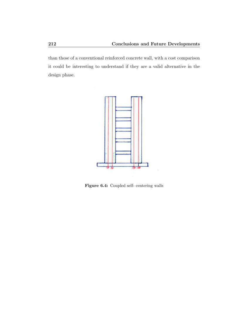
212 Conclusions and Future Developments
than those of a conventional reinforced concrete wall, with a cost comparison
it could be interesting to understand if they are a valid alternative in the
design phase.
Figure 6.4: Coupled self- centering walls

List of Figures
2.1 Sequence of operations for FBD methodology . . . . . . . . . 13
2.2 Simplified force-displacement response of elastic and inelastic
systems under seismic excitation . . . . . . . . . . . . . . . . . 17
2.3 Force distribution over the height of the building: a) con-
sidering actual mode shape, b) considering semplified linear
distribution . . . . . . . . . . . . . . . . . . . . . . . . . . . . 19
2.4 Force-displacement relationship . . . . . . . . . . . . . . . . . 24
2.5 Possibles definition of yield and ultimate displacement . . . . 28
2.6 Fundamentals of DDBD, Priestley . . . . . . . . . . . . . . . . 32
2.7 Sequence of operations for DDBD methodology . . . . . . . . 33
2.8 Schematic representation for computing equivalent viscous damp-
ing coefficient . . . . . . . . . . . . . . . . . . . . . . . . . . . 44
2.9 Bilinear approximation of curvature distribution . . . . . . . . 48
2.10 Simplified capacity design moment and shear envelopes for
cantilever walls, Priestley . . . . . . . . . . . . . . . . . . . . . 51
2.11 Flexural response and associative curvature for precast jointed
wall (a) and equivalent monolithic wall (b) . . . . . . . . . . . 54
3.1 Restoring behavior due to gap opening . . . . . . . . . . . . . 63

214 LIST OF FIGURES
3.2 Examples of Self-Centering System: (a) Hybrid moment frame,
(b) Unbonded post-tensioned precast wall . . . . . . . . . . . 64
3.3 Expected flag-shaped behavior of a generic self-centering sys-
tem, [12] . . . . . . . . . . . . . . . . . . . . . . . . . . . . . . 64
3.4 Possibles behaviors along the horizontal joints of a precast wall 66
3.5 Base-Shear-Roof-Drift relationship of an unbonded post-tensioned
precast wall, Kurama . . . . . . . . . . . . . . . . . . . . . . . 69
3.6 Hysteretic loop under cyclic load, Kurama . . . . . . . . . . . 69
3.7 Roof-drift time-history, Kurama . . . . . . . . . . . . . . . . . 70
3.8 Unbonded post-tensioned precast jointed wall . . . . . . . . . 71
3.9 U-shaped flexural plate (UFPs) . . . . . . . . . . . . . . . . . 71
3.10 Unbonded Post-Tensioned Hybrid Wall: general layout and
displaced configuration . . . . . . . . . . . . . . . . . . . . . . 73
3.11 Unbonded post-tensioned precast walls with spread viscous
dampers . . . . . . . . . . . . . . . . . . . . . . . . . . . . . . 74
3.12 Propped rocking wall: general layout and deformed shape, [11] 76
3.13 Hybrid PT-CIP wall behavior, [12] . . . . . . . . . . . . . . . 79
3.14 Base joint: exaggerated deformed shape at ∆d . . . . . . . . . 86
3.15 Stress-strain relationship for PT strands (on the left) and ED
bars (on the right) . . . . . . . . . . . . . . . . . . . . . . . . 88
3.16 Base joint: free body diagram at ∆d . . . . . . . . . . . . . . . 89
3.17 Idealized flag-shaped hysteretic loop . . . . . . . . . . . . . . . 92
4.1 Examples of models developed by University of Notre Dame:
(a) is the finite element model, (b) is the fiber element model . 98
4.2 Global view of the test building . . . . . . . . . . . . . . . . . 102
4.3 Floor plan of the prototype building . . . . . . . . . . . . . . . 104
4.4 Flooring system at different levels . . . . . . . . . . . . . . . . 105

LIST OF FIGURES 215
4.5 Elevation of the unbonded post-tensioned jointed precast wall,
[10] . . . . . . . . . . . . . . . . . . . . . . . . . . . . . . . . . 107
4.6 Erection of the unbonded post-tensioned jointed precast wall . 108
4.7 Ruaumoko model, PRESSS report . . . . . . . . . . . . . . . . 113
4.8 Foundation spring hysteretic behavior . . . . . . . . . . . . . . 116
4.9 Force-Displacement relationship of the UFPs, PRESSS report 119
4.10 Al-Bermani Hysteretic Rule . . . . . . . . . . . . . . . . . . . 120
4.11 PRESSS results, test maximum displacement profiles . . . . . 125
4.12 PRESSS results, pushover curve . . . . . . . . . . . . . . . . . 126
4.13 Elevation of the proposed model . . . . . . . . . . . . . . . . . 129
4.14 Base of the proposed model . . . . . . . . . . . . . . . . . . . 130
4.15 Differents model of the re-centering behavior . . . . . . . . . . 134
4.16 Hysteretic rule of the PT springs . . . . . . . . . . . . . . . . 135
4.17 Wen hysteretic rule, [29] . . . . . . . . . . . . . . . . . . . . . 137
4.18 Nonlinear shear-displacement response of UFP links under
cyclic loads: (a) USCS units, (b) SI units . . . . . . . . . . . . 138
4.19 Response spectra comparison . . . . . . . . . . . . . . . . . . 140
4.20 Response spectrum compatible time histories . . . . . . . . . . 141
4.21 Exaggerated displaced configuration of the proposed model . . 143
4.22 Force-displacement relationships for different link elements in
the proposed model under a simulated ground motion . . . . . 144
4.23 Proposed Model Base moment-Top displacement relationship,
pushover results . . . . . . . . . . . . . . . . . . . . . . . . . . 146
4.24 Full cycle hysteresis loop . . . . . . . . . . . . . . . . . . . . . 147
4.25 Floor Displacements time histories . . . . . . . . . . . . . . . 149
4.26 Top Displacement time history . . . . . . . . . . . . . . . . . . 150
4.27 Base moment hysteresis loop . . . . . . . . . . . . . . . . . . . 151

216 LIST OF FIGURES
5.1 Global view of Civic Center . . . . . . . . . . . . . . . . . . . 156
5.2 Global view of Civic Center . . . . . . . . . . . . . . . . . . . 157
5.3 Typical system elevation . . . . . . . . . . . . . . . . . . . . . 158
5.4 Typical tower framing plan . . . . . . . . . . . . . . . . . . . . 158
5.5 Proposed plan . . . . . . . . . . . . . . . . . . . . . . . . . . . 160
5.6 Site-Specific Response Spectrum . . . . . . . . . . . . . . . . . 161
5.7 Idealized hysteretic damping calculation . . . . . . . . . . . . 167
5.8 Correction factors to be applied to the area-based equivalent
viscous damping ratio, Priestley [16] . . . . . . . . . . . . . . 168
5.9 Response displacement spectra . . . . . . . . . . . . . . . . . . 170
5.10 Wall base layout of the model of a hybrid wall . . . . . . . . . 176
5.11 Response spectra comparison . . . . . . . . . . . . . . . . . . 178
5.12 Case study, response spectrum compatible time histories . . . 179
5.13 Case study, full cycle hysteresis loop, first iteration . . . . . . 180
5.14 Case study, full cycle hysteresis loop, final iteration . . . . . . 182
5.15 Case study, Base moment-Top displacement relationship, pushover
results . . . . . . . . . . . . . . . . . . . . . . . . . . . . . . . 184
5.16 Floor Displacements time histories . . . . . . . . . . . . . . . 186
5.17 Force-displacement relationships for different link elements un-
der the Loma Prieta ground acceleration . . . . . . . . . . . . 187
5.18 Response displacement spectra . . . . . . . . . . . . . . . . . . 192
5.19 Amplified moment along the height . . . . . . . . . . . . . . . 193
5.20 Moment curvature analysis: (a) nominal strength, (b) over-
strength . . . . . . . . . . . . . . . . . . . . . . . . . . . . . . 195
5.21 Amplified shear along the height . . . . . . . . . . . . . . . . . 196
6.1 Configuration of unbonded post-tensioned concrete wall with
central bearing . . . . . . . . . . . . . . . . . . . . . . . . . . 201

LIST OF FIGURES 217
6.2 Influence of viscous dampers in the displacement response . . 207
6.3 Self-centering wall with shear keys . . . . . . . . . . . . . . . . 211
6.4 Coupled self- centering walls . . . . . . . . . . . . . . . . . . . 212

218 LIST OF FIGURES

List of Tables
2.1 Fundamental periods of wall buildings . . . . . . . . . . . . . 26
4.1 PRESSS test building scale factors, [3] . . . . . . . . . . . . . 103
4.2 Results from the DDBD procedure . . . . . . . . . . . . . . . 110
4.3 Comparison of the design base shear obtained from DDBD
and FBD, [26] . . . . . . . . . . . . . . . . . . . . . . . . . . . 110
4.4 PRESSS test building, wall member parameters . . . . . . . . 114
4.5 PRESSS test building, PT springs parameters . . . . . . . . . 118
4.6 PRESSS test building, UFP springs parameters . . . . . . . . 122
4.7 Proposed Model, wall member parameters . . . . . . . . . . . 131
4.8 Proposed Model, foundation link parameters . . . . . . . . . . 132
4.9 Proposed model, PT links parameters . . . . . . . . . . . . . . 136
4.10 Proposed Model, UFP link parameters . . . . . . . . . . . . . 138
5.1 Uniformly Distributed Loads . . . . . . . . . . . . . . . . . . . 162
5.2 Material Properties . . . . . . . . . . . . . . . . . . . . . . . . 163
5.3 Design displacement at each level . . . . . . . . . . . . . . . . 164
5.4 ETABS Model - Properties of the Components . . . . . . . . . 177
5.5 Material Quantities . . . . . . . . . . . . . . . . . . . . . . . . 181
5.6 ETABS Model - Properties of the Components . . . . . . . . . 182
5.7 Material Properties for a Cantilever Concrete Wall . . . . . . 189

220 LIST OF TABLES
5.8 Wall Displacement for a Cantilever Concrete Wall . . . . . . . 190
6.1 ETABS Model Enhanced Wall- Properties of the Components 205

Bibliography
[1] Baird A., Smith T., Palermo A., Pampanin S., Experimental and numer-
ical Study of U-shape Flexural Plate (UFP) Dissipators, Conference of
New Zealand Society For Earthquake Engineering (NZSEE), Aukland,
Paper No P2, 2014.
[2] Chancellor N.B., Eatherton M.R., Roke D.A., Akbas T., Self-Centering
Seismic Lateral Force Resisting Systems: High Performance Structures
for the City of Tomorrow, Buildings Journal, 18/09/2014.
[3] Conley J., Sritharan S., Priestley M.J.N., Precast Seismic Structural
Systems PRESSS-3: the Five-Story Precast Test Building vol. 3-j: Wall
Direction Response, University of California San Diego, Final Report
Submitted to the Precast/Prestressed Concrete Institute, July 2002.
[4] Henry R.S., Self-centering Precast Concrete Walls for Buildings in Re-
gions with Low to High Seismicity, PhD Thesis, Department of Civil
and Environmental Engineering, The University of Auckland, 2011.
[5] Kurama Y.C., Seismic Analysis, Behavior and Design of Unbonded
Post-Tensioned Precast Concrete Walls, PhD Thesis, Department of
Civil and Environmental Engineering, Lehigh University (Bethlem,
Pennsylvania), 1997.

222 BIBLIOGRAPHY
[6] Kurama Y.C., Pessiki S., Sause R., Seismic Behavior and Design of Un-
bonded Post-Tensioned Precast Concrete Walls, PCI JOURNAL, May-
June 1999, pp. 72-89.
[7] Kurama Y.C., Unbonded Post-Tensioned Precast Concrete Walls With
Supplemental Viscous Damping, ACI Structural Journal, vol 97, 2000,
pp. 648-658.
[8] Kurama Y.C., Hybrid Post-Tensioned Precast Concrete Walls For Use
in Seismic Regions, PCI JOURNAL, September-October 2002, pp. 36-
59.
[9] Kurama Y.C., Seismic Design of Partially Post-Tensioned Precast Con-
crete Walls, PCI JOURNAL, July-August 2005, pp. 100-125.
[10] Nakaki S.D., Stanton J.F., Sritharan S., An Overview of the PRESSS
Five-Story Precast Test Building, PCI JOURNAL, March-April 1999,
pp. 26-39.
[11] Nicknam A., Filiatrault A., Direct Displacement-Based Seismic Design
of Propped Rocking Walls, Earthquake Spectra, vol 31 No. 1, 2015, pp.
179-196.
[12] Panian L., Steyer M., Tipping S., Post-Tensioned Concrete Walls For
Seismic Resistance, PTI JOURNAL, vol 5 No.1, July 2007, pp. 7-16.
[13] Panian L., Steyer M., Tipping S., Post-Tensioned Shotcrete Shearwalls,
American Concrete Institute, vol 29 No.10, October 2007, pp. 43-49.
[14] Priestley M.J.N., Performance-Based Seismic Design, 12th World Con-
ference on Earthquake Engineering, Aukland, No. 2831, 2000.

BIBLIOGRAPHY 223
[15] Priestley M. N., Amaris, A. D., Dynamic Amplification of Seismic Mo-
ments and Shear Forces in Cantilever Walls, IUSS Press, 2002.
[16] Priestley M.J.N., Direct Displacement-Based Design of Pre-
cast/Prestressed Concrete Buildings, PCI JOURNAL, November-
December 2002, pp. 66-79.
[17] Priestley M.J.N., Calvi G.M., Kowalsky M.J., Displacement-Based Seis-
mic Design of Structures, IUSS Press, Pavia, 2007.
[18] Rahman M.A., Performance-Based Seismic Analysis And Design Im-
provements Of Two Precast Concrete Structural Systems, Retrospective
Theses and Dissertations, Iowa State University, 2008.
[19] Rahman M.A., Sritharan S., Force-Based vs. Displacement-Based Design
of Jointed Precast Prestressed Wall Systems, Civil, Construction and
Evironmental Engineering Technical Report, Paper No. 6, Iowa State
University, 2011.
[20] Reitherman R.K., Five Major Themes In the History of Earthquake En-
gineering, 15th World Conference on Earthquake Engineering, Lisbon,
Portugal, 2012.
[21] Sarkisian M., Lee P., Garai R., Tsui A., Controlling Wind in Tall and
Flexible Structure With Viscous Damping Devices, SEAOC 2015 Con-
vention Proceedings, 2015.
[22] Smith R.S.H, Tso W.K., Inconsistency of Force-Based Design Procedure,
JSEE, Vol.4 No.1, 2002.

224 BIBLIOGRAPHY
[23] Smith B.J., Kurama Y.C., McGinnis M.J., Hybrid Precast Wall Systems
For Seismic Region, Structural Engineering Research Report, University
of Notre Dame (Notre Dame, Indiana), 2012.
[24] Smith B.J., Kurama Y.C., McGinnis M.J., Seismic Design Guidelines
for Special Hybrid Precast Concrete Shear Walls, Structural Engineering
Research Report, University of Notre Dame (Notre Dame, Indiana),
2012.
[25] Sritharan S., Priestley M.J.N., Seible F., Igarashi A., A Five-Story Pre-
cast Concrete Test Building For Seismic Conditions - An Overview, 12th
World Conference on Earthquake Engineering, Aukland, No. 1299, 2000.
[26] Sritharan S., Pampanin S., Conley J., Precast Seismic Structural Sys-
tems PRESSS-3: the Five-Story Precast Test Building vol. 3-03: Design
Verification, Instrumentation & Test Procedures, Final Report Submit-
ted to the Precast/Prestressed Concrete Institute, December 2002.
[27] Stanton J.F., Nakaki S.D., Precast Seismic Structural Systems PRESSS-
3: the Five-Story Precast Test Building vol. 3-09: Design Guidelines For
Precast Concrete Seismic Structural Systems, The University of Wash-
ington and The Nakaki Bashaw Group, Inc., February 2002.
[28] Stevenson M., Panian L., Korolyk M., Mar D., Post-Tensioned Concrete
Walls and Frames for Seismic-Resistance A Case Study of the David
Brower Center, SEAOC 2008 Convention Proceedings, 2008.
[29] CSI Analysis Reference Manual For SAP2000, ETABS, SAFE and
CSiBridge, Computer & Structures Inc., Berkeley (California), 2015.

BIBLIOGRAPHY 225
[30] ASCE 7-10. ASCE/SEI 7-10: Minimum Design Loads For Buildings
and Other Structures, American Society of Civil Engineers, 2010.
[31] EN 1998. Eurocode 8: Design of structures for earthquake resistance,
European Committee for Standardisation (CEN), 2005.