PointPWC-Net: Cost Volume on Point Cloudsfor (Self-)Supervised Scene Flow Estimation

Wenxuan Wu1, Zhi Yuan Wang2, Zhuwen Li2, Wei Liu2, and Li Fuxin1

1 CORIS Institute, Oregon State University{wuwen,lif}@oregonstate.edu

2 Nuro, Inc.

Abstract. We propose a novel end-to-end deep scene flow model, calledPointPWC-Net, that directly processes 3D point cloud scenes with largemotions in a coarse-to-fine fashion. Flow computed at the coarse levelis upsampled and warped to a finer level, enabling the algorithm to ac-commodate for large motion without a prohibitive search space. We in-troduce novel cost volume, upsampling, and warping layers to efficientlyhandle 3D point cloud data. Unlike traditional cost volumes that requireexhaustively computing all the cost values on a high-dimensional grid,our point-based formulation discretizes the cost volume onto input 3Dpoints, and a PointConv operation efficiently computes convolutions onthe cost volume. Experiment results on FlyingThings3D and KITTI out-perform the state-of-the-art by a large margin. We further explore novelself-supervised losses to train our model and achieve comparable resultsto state-of-the-art trained with supervised loss. Without any fine-tuning,our method also shows great generalization ability on the KITTI SceneFlow 2015 dataset, outperforming all previous methods. The code is re-leased at https://github.com/DylanWusee/PointPWC.

Keywords: Cost Volume; Self-supervision; Coarse-to-fine; Scene Flow.

1 Introduction

Scene flow is the 3D displacement vector between each surface point in twoconsecutive frames. As a fundamental tool for low-level understanding of theworld, scene flow can be used in many 3D applications including autonomousdriving. Traditionally, scene flow was estimated directly from RGB data [45, 44,72, 74]. But recently, due to the increasing application of 3D sensors such asLiDAR, there is interest on directly estimating scene flow from 3D point clouds.

Fueled by recent advances in 3D deep networks that learn effective featurerepresentations directly from point cloud data, recent work adopt ideas from2D deep optical flow networks to 3D to estimate scene flow from point clouds.FlowNet3D [36] operates directly on points with PointNet++ [54], and proposesa flow embedding which is computed in one layer to capture the correlationbetween two point clouds, and then propagates it through finer layers to estimatethe scene flow. HPLFlowNet [20] computes the correlation jointly from multiplescales utilizing the upsampling operation in bilateral convolutional layers.

2 W. Wu et al.

Cost Volume; Upsample;Warping; Scene Flow Predictor.

Cost Volume; Upsample;Warping; Scene Flow Predictor.

Cost Volume; Upsample;Warping; Scene Flow Predictor.

Cost Volume; Upsample;Warping; Scene Flow Predictor.

(b)

P 𝑄𝑆𝐹

Novel Upsample Layer

Novel Warping Layer Novel Cost Volume Layer

(a)

Scene Flow Predictor

𝐹𝑖𝑛𝑒𝑟 𝐹𝑙𝑜𝑤

𝐶𝑜𝑎𝑟𝑠𝑒 𝐹𝑙𝑜𝑤

Fig. 1. (a) illustrates how the pyramid features are used by the novel cost volume, warp-ing, and upsampling layers in one level. (b) shows the overview structure of PointPWC-Net. At each level, PointPWC-Net first warps features from the first point cloud usingthe upsampled scene flow. Then, the cost volume is computed using features from thewarped first point cloud and the second point cloud. Finally, the scene flow predictorpredicts finer flow at the current level using features from the first point cloud, the costvolume, and the upsampled flow. (Best viewed in color)

An important piece in deep optical flow estimation networks is the cost vol-ume [31, 81, 65], a 3D tensor that contains matching information between neigh-boring pixel pairs from consecutive frames. In this paper, we propose a novellearnable point-based cost volume where we discretize the cost volume to inputpoint pairs, avoiding the creation of a dense 4D tensor if we naively extend fromthe image to point cloud. Then we apply the efficient PointConv layer [80] onthis irregularly discretized cost volume. We experimentally show that it outper-forms previous approaches for associating point cloud correspondences, as wellas the cost volume used in 2D optical flow. We also propose efficient upsamplingand warping layers to implement a coarse-to-fine flow estimation framework.

As in optical flow, it is difficult and expensive to acquire accurate scene flowlabels for point clouds. Hence, beyond supervised scene flow estimation, we alsoexplore self-supervised scene flow which does not require human annotations.We propose new self-supervised loss terms: Chamfer distance [14], smoothnessconstraint and Laplacian regularization. These loss terms enable us to achievestate-of-the-art performance without any supervision.

We conduct extensive experiments on FlyingThings3D [44] and KITTI SceneFlow 2015 [47, 46] datasets with both supervised loss and the proposed self-supervised losses. Experiments show that the proposed PointPWC-Net outper-forms all previous methods by a large margin. The self-supervised version iscomparable with some of the previous supervised methods on FlyingThings3D,such as SPLATFlowNet [63]. On KITTI where supervision is not available, ourself-supervised version achieves better performance than the supervised versiontrained on FlyingThings3D, far surpassing state-of-the-art. We also ablate eachcritical component of PointPWC-Net to understand their contributions.

The key contributions of our work are:• We propose a novel learnable cost volume layer that performs convolution

on the cost volume without creating a dense 4D tensor.•With the novel learnable cost volume layer, we present a novel model, called

PointPWC-Net, that estimates scene flow from two consecutive point clouds in

PointPWC-Net 3

a coarse-to-fine fashion.• We introduce self-supervised losses that can train PointPWC-Net without

any ground truth label. To our knowledge, we are among the first to proposesuch an idea in 3D point cloud deep scene flow estimation.• We achieve state-of-the-art performance on FlyingThing3D and KITTI

Scene Flow 2015, far surpassing previous state-of-the-art.

2 Related Work

Deep Learning on Point Clouds. Deep learning methods on 3D point cloudshave gained more attention in the past several years. Some latest work [57, 53,54, 63, 68, 25, 19, 73, 34] directly take raw point clouds as input. [57, 53, 54] use ashared multi-layer perceptron (MLP) and max pooling layer to obtain featuresof point clouds. Other work [61, 30, 79, 22, 78, 80] propose to learn continuousconvolutional filter weights as a nonlinear function from 3D point coordinates,approximated with MLP. [22, 80] use a density estimation to compensate thenon-uniform sampling, and [80] significantly improves the memory efficiency bya change of summation trick, allowing these networks to scale up and achievingcomparable capabilities with 2D convolution.Optical Flow Estimation. Optical flow estimation is a core computer visionproblem and has many applications. Traditionally, top performing methods oftenadopt the energy minimization approach [24] and a coarse-to-fine, warping-basedmethod [4, 8, 7]. Since FlowNet [13], there were many recent work using a deepnetwork to learn optical flow. [28] stacks several FlowNets into a larger one.[56] develops a compact spatial pyramid network. [65] integrates the widely usedtraditional pyramid, warping, and cost volume technique into CNNs for opticalflow, and outperform all the previous methods with high efficiency. We utilizeda basic structure similar to theirs but proposed novel cost volume, warping andupsampling layers appropriate for point clouds.Scene Flow Estimation. 3D scene flow is first introduced by [72]. Manyworks [26, 45, 75] estimate scene flow using RGB data. [26] introduces a vari-ational method to estimate scene flow from stereo sequences. [45] proposes anobject-level scene flow estimation approach and introduces a dataset for 3D sceneflow. [75] presents a piecewise rigid scene model for 3D scene flow estimation.

Recently, there are some works [12, 71, 70] that estimate scene flow directlyfrom point clouds using classical techniques. [12] introduces a method that for-mulates the scene flow estimation problem as an energy minimization problemwith assumptions on local geometric constancy and regularization for motionsmoothness. [71] proposes a real-time four-steps method of constructing occu-pancy grids, filtering the background, solving an energy minimization problem,and refining with a filtering framework. [70] further improves the method in [71]by using an encoding network to learn features from an occupancy grid.

In some most recent work [78, 36, 20], researchers attempt to estimate sceneflow from point clouds using deep learning in a end-to-end fashion. [78] usesPCNN to operate on LiDAR data to estimate LiDAR motion. [36] introduces

4 W. Wu et al.

FlowNet3D based on PointNet++ [54]. FlowNet3D uses a flow embedding layerto encode the motion of point clouds. However, it requires encoding a large neigh-borhood in order to capture large motions. [20] presents HPLFlowNet to esti-mate the scene flow using Bilateral Convolutional Layers(BCL), which projectsthe point cloud onto a permutohedral lattice. [3] estimates scene flow with anetwork that jointly predicts 3D bounding boxes and rigid motions of objects orbackground in the scene. Different from [3], we do not require the rigid motionassumption and segmentation level supervision to estimate scene flow.

Self-supervised Scene Flow. There are several recent works [35, 82, 87, 32, 27]which jointly estimate multiple tasks, i.e. depth, optical flow, ego-motion andcamera pose without supervision. They take 2D images as input, which haveambiguity when used in scene flow estimation. In this paper, we investigate self-supervised learning of scene flow from 3D point clouds with our PointPWC-Net.Concurrently, Mittal et al. [49] introduced Nearest Neighbor(NN) Loss and CycleConsistency Loss to self-supervised scene flow estimation from point clouds.However, they does not take the local structure properties of 3D point cloudsinto consideration. In our work, we propose to use smoothness and Laplaciancoordinates to preserve local structure for scene flow.

Traditional Point Cloud Registration. Point cloud registration has beenextensively studied well before deep learning [21, 66]. Most of the work [10, 18,23, 43, 48, 60, 69, 85] only works when most of the motion in the scene is globallyrigid. Many methods are based on the iterative closest point(ICP) [5] and itsvariants [52]. Several works [1, 50, 29, 6] deal with non-rigid point cloud regis-tration. Coherent Point Drift(CPD) [50] introduces a probabilistic method forboth rigid and non-rigid point set registration. However, the computation over-head makes it hard to apply on real world data in real-time. Many algorithmsare proposed to extend the CPD method [41, 51, 38, 86, 17, 42, 15, 2, 16, 40, 39, 33,67, 59, 11, 37, 84, 76, 83, 55]. Some algorithms require additional information forpoint set registration. The work [59, 11] takes the color information along withthe spatial location into account. [1] requires meshes for non-rigid registration.In [55], the regression and clustering for point set registration in a Bayesianframework are presented. All the aforementioned work require optimization atinference time, which has significantly higher computation cost than our methodwhich run in a fraction of a second during inference.

3 Approach

To compute optical flow with high accuracy, one of the most important com-ponents is the cost volume. In 2D images, the cost volume can be computedby aggregating the cost in a square neighborhood on a grid. However, comput-ing cost volume across two point clouds is difficult since 3D point clouds areunordered with a nonuniform sampling density. In this section, we introduce anovel learnable cost volume layer, and use it to construct a deep network withthe help of other auxiliary layers that outputs high quality scene flow.

PointPWC-Net 5

3.1 The Cost Volume Layer

As one of the key components of optical flow estimation, most state-of-the-artalgorithms, both traditional [64, 58] and modern deep learning based ones [65,81, 9], use the cost volume to estimate optical flow. However, computing costvolumes on point clouds is still an open problem. There are several works [36, 20]that compute some kind of flow embedding or correlation between point clouds.[36] proposes a flow embedding layer to aggregate feature similarities and spatialrelationships to encode point motions. However, the motion information betweenpoints can be lost due to the max pooling operation in the flow embeddinglayering. [20] introduces a CorrBCL layer to compute the correlation betweentwo point clouds, which requires to transfer two point clouds onto the samepermutohedral lattice.

To address these issues, we present a novel learnable cost volume layer di-rectly on the features of two point clouds. Suppose fi ∈ Rc is the feature forpoint pi ∈ P and gj ∈ Rc the feature for point qj ∈ Q, the matching cost betweenpi and qj can be defined as:

Cost(pi, qj) = h(fi, gj , qj , pi) (1)

= MLP (concat(fi, gj , qj − pi)) (2)

Where concat stands for concatenation. In our network, the feature fi and gj areeither the raw coordinates of the point clouds, or the convolution output fromprevious layers. The intuition is that, as a universal approximator, MLP shouldbe able to learn the potentially nonlinear relationship between the two points.Due to the flexibility of the point cloud, we also add a direction vector (qj − pi)to the computation besides the point features fi and gj .

Once we have the matching costs, they can be aggregated as a cost volume forpredicting the movement between two point clouds. In 2D images, aggregatingthe cost is simply by applying some convolutional layers as in PWC-Net [65].However, traditional convolutional layers can not be applied directly on pointclouds due to their unorderness. [36] uses max-pooing to aggregate features in thesecond point cloud. [20] uses CorrBCL to aggregate features on a permutohedrallattice. However, their methods only aggregate costs in a point-to-point manner,which is sensitive to outliers. To obtain robust and stable cost volumes, in thiswork, we propose to aggregate costs in a patch-to-patch manner similar to thecost volumes on 2D images [31, 65].

For a point pc in P , we first find a neighborhood NP (pc) around pc in P . Foreach point pi ∈ NP (pc), we find a neighborhood NQ(pi) around pi in Q. Thecost volume for pc is defined as:

CV (pc) =∑

pi∈NP (pc)

WP (pi, pc)∑

qj∈NQ(pi)

WQ(qj , pi) cost(qj , pi) (3)

WP (pi, pc) = MLP (pi − pc) (4)

WQ(qj , pi) = MLP (qj − pi) (5)

6 W. Wu et al.

𝑝

𝑁 (𝑝 )𝑁 (𝑝 )

𝑃𝑜𝑖𝑛𝑡 𝐶𝑙𝑜𝑢𝑑 𝑃

𝑃𝑜𝑖𝑛𝑡 𝐶𝑙𝑜𝑢𝑑 𝑄𝑞 − 𝑝

𝑝 − 𝑝

: 𝑒𝑙𝑒𝑚𝑒𝑛𝑡 − 𝑤𝑖𝑠𝑒 𝑝𝑟𝑜𝑑𝑢𝑐𝑡

𝐹 : 𝑁 × 𝐶

𝐹 : 𝑁 × 𝐶

𝑃: 𝑁 × 3

𝑄: 𝑁 × 3

𝑁(𝑝

)

𝑐𝑜𝑛𝑐𝑎𝑡 𝑓 , 𝑔 , 𝑞 − 𝑝 :

𝑁 × 𝐾 × (2𝐶 + 3)

𝑞 − 𝑝 :

𝑁 × 𝐾 × 3 𝑀𝐿

𝑃

𝑀𝐿

𝑃 ℎ 𝑓 , 𝑔 , 𝑞 , 𝑝 :

𝑁 × 𝐾 × 𝐷

𝑊 𝑞 , 𝑝 :

𝑁 × 𝐾 × 𝐷

𝑃𝑜𝑖𝑛𝑡-𝑡𝑜-𝑃𝑎𝑡𝑐ℎ𝐶𝑜𝑠𝑡:𝑁 × 𝐷

𝑠𝑢𝑚

𝑁(𝑝

)

𝑀𝐿

𝑃 𝑊 𝑝 , 𝑝 :𝑁 × 𝐾 × 𝐷

𝑃𝑎𝑡𝑐ℎ-𝑡𝑜-𝑃𝑎𝑡𝑐ℎ𝐶𝑜𝑠𝑡 𝑉𝑜𝑙𝑢𝑚𝑒:

𝑁 × 𝐷

𝑠𝑢𝑚

𝑝 − 𝑝 :𝑁 × 𝐾 × 3

𝑁 × 𝐾 × 𝐷

a Grouping 𝑏 Cost Volume Layer

Fig. 2. (a) Grouping. For a point pc, we form its K-NN neighborhoods in each pointcloud as NP (pc) and NQ(pc) for cost volume aggregation. We first aggregate the costfrom the patchNQ(pc) in point cloudQ. Then, we aggregate the cost from patchNP (pc)in the point cloud P . (b) Cost Volume Layer. The features of neighboring points inNQ(pc) are concatenated with the direction vector (qi − pc) to learn a point-to-patchcost between pc and Q with PointConv. Then the point-to-patch costs in NP (pc) arefurther aggregated with PointConv to construct a patch-to-patch cost volume

Where WP (pi, pc) and WQ(qj , pi) are the convolutional weights w.r.t the direc-tion vectors that are used to aggregate the costs from the patches in P and Q. Itis learned as a continuous function of the directional vectors (qi − pc) ∈ R3 and(qj − pi) ∈ R3, respectively with an MLP, as in [80] and PCNN [78]. The outputof the cost volume layer is a tensor with shape (n1, D), where n1 is the numberof points in P , and D is the dimension of the cost volume, which encodes allthe motion information for each point. The patch-to-patch idea used in the costvolume is illustrated in Fig. 2.

There are two major differences between this cost volume for scene flow of3D point clouds and conventional 2D cost volumes for stereo and optical flow.The first one is that we introduce a learnable function cost(·) that can dynam-ically learn the cost or correlation within the point cloud structures. Ablationstudies in Sec.5.3 show that this novel learnable design achieve better resultsthan traditional cost volume [65] in scene flow estimation. The second one isthat this cost volume is discretized irregularly on the two input point cloudsand their costs are aggregated with point-based convolution. Previously, in or-der to compute the cost volume for optical flow in a d × d area on a W × H2D image, all the values in a d2 ×W ×H tensor needs to be populated, whichis already slow to compute in 2D, but would be prohibitively costly in the 3Dspace. With (volumetric) 3D convolution, one needs to search a d3 area to ob-tain a cost volume in 3D space. Our cost volume discretizes on input points andavoids this costly operation, while essentially creating the same capabilities toperform convolutions on the cost volume. With the proposed cost volume layer,we only need to find two neighborhoods NP (pc) and NQ(pi) of size K, which ismuch cheaper and does not depend on the number of points in a point cloud. Inour experiments, we fix |NP (pc)| = |NQ(pi)| = 16. If a larger neighborhood isneeded, we could subsample the neighborhood which would bring it back to thesame speed. This subsampling operation is only applicable to the sparse pointcloud convolution and not possible for conventional volumetric convolutions. Weanticipate this novel cost volume layer to be widely useful beyond scene flowestimation. Table 2 shows that it is better than [36]’s MLP+Maxpool strategy.

PointPWC-Net 7

3.2 PointPWC-Net

Given the proposed learnable cost volume layer, we construct a deep networkfor scene flow estimation. As demonstrated in 2D optical flow estimation, oneof the most effective methods for dense estimation is the coarse-to-fine struc-ture. In this section, we introduce some novel auxiliary layers for point cloudsthat construct a coarse-to-fine network for scene flow estimation along with theproposed learnable cost volume layer. The network is called “PointPWC-Net”following [65].

As shown in Fig.1, PointPWC-Net predicts dense scene flow in a coarse-to-fine fashion. The input to PointPWC-Net is two consecutive point clouds,P = {pi ∈ R3}n1

i=1 with n1 points, and Q = {qj ∈ R3}n2j=1 with n2 points. We

first construct a feature pyramid for each point cloud. Afterwards, we build acost volume using features from both point clouds at each layer. Then, we usethe feature from P , the cost volume, and the upsampled flow to estimate thefiner scene flow. We take the predicted scene flow as the coarse flow, upsample itto a finer flow, and warp points from P onto Q. Note that both the upsamplingand the warping layers are efficient with no learnable parameters.Feature Pyramid from Point Cloud. To estimate scene flow with high accu-racy, we need to extract strong features from the input point clouds. We generatean L-level pyramid of feature representations, with the top level being the inputpoint clouds, i.e., l0 = P/Q. For each level l, we use furthest point sampling [54]to downsample the points by a factor of 4 from previous level l − 1, and usePointConv [80] to perform convolution on the features from level l− 1. As a re-sult, we can generate a feature pyramid with L levels for each input point cloud.After this, we enlarge the receptive field at level l of the pyramid by upsamplingthe feature in level l + 1 and concatenate it to the feature at level l.Upsampling Layer. The upsampling layer can propagate the scene flow esti-mated from a coarse layer to a finer layer. We use a distance based interpolationto upsample the coarse flow. Let P l be the point cloud at level l, SF l be theestimated scene flow at level l, and pl−1 be the point cloud at level l−1. For eachpoint pl−1i in the finer level point cloud P l−1, we can find its K nearest neighborsN(pl−1i ) in its coarser level point cloud P l. The interpolated scene flow of finerlevel SF l−1 is computed using inverse distance weighted interpolation:

SF l−1(pi) =

∑kj=1 w(pl−1

i , plj)SFl(plj)∑k

j=1 w(pl−1i , plj)

(6)

where w(pl−1i , plj) = 1/d(pl−1i , plj), pl−1i ∈ P l−1, and plj ∈ N(pl−1i ). d(pl−1i , plj) is

a distance metric. We use Euclidean distance in this work.Warping Layer. Warping would “apply” the computed flow so that only theresidual flow needs to be estimated afterwards, hence the search radius can besmaller when constructing the cost volume. In our network, we first up-samplethe scene flow from the previous coarser level and then warp it before computingthe cost volume. Denote the upsampled scene flow as SF = {sfi ∈ R3}n1

i=1,and the warped point cloud as Pw = {pw,i ∈ R3}n1

i=1. The warping layer is

8 W. Wu et al.

simply an element-wise addition between the upsampled and computed sceneflow Pw = {pw,i = pi + sfi|pi ∈ P, sfi ∈ SF}n1

i=1. A similar warping operationis used for visualization to compare the estimated flow with the ground truthin [36, 20], but not used in coarse-to-fine estimation. [20] uses an offset strategyto reduce search radius which is specific to the permutohedral lattice.Scene Flow Predictor. In order to obtain a flow estimate at each level, aconvolutional scene flow predictor is built as multiple layers of PointConv andMLP. The inputs of the flow predictor are the cost volume, the feature of thefirst point cloud, the up-sampled flow from previous layer and the up-sampledfeature of the second last layer from previous level’s scene flow predictor, whichwe call the predictor feature. The output is the scene flow SF = {sfi ∈ R3}n1

i=1

of the first point cloud P . The first several PointConv layers are used to mergethe feature locally, and the following MLP is used to estimate the scene flow oneach point. We keep the flow predictor structure at different levels the same, butthe parameters are not shared.

4 Training Loss Functions

In this section, we introduce two loss functions to train PointPWC-Net for sceneflow estimation. One is the standard multi-scale supervised training loss, whichhas been explored in deep optical flow estimation [65] in 2D images. We usethis supervised loss to train the model for fair comparison with previous sceneflow estimation work, including FlowNet3D [36] and HPLFlowNet [20]. Due tothat acquiring densely labeled 3D scene flow dataset is extremely hard, we alsopropose a novel self-supervised loss to train our PointPWC-Net without anysupervision.

4.1 Supervised Loss

We adopt the multi-scale loss function in FlowNet [13] and PWC-Net [65] as asupervised learning loss to demonstrate the effectiveness of the network structureand the design choice. Let SF lGT be the ground truth flow at the l-th level. The

multi-scale training loss `(Θ) =∑Ll=l0

αl∑p∈P

∥∥SF lΘ(p)− SF lGT (p)∥∥2

is usedwhere ‖·‖2 computes the L2-norm, αl is the weight for each pyramid level l, andΘ is the set of all the learnable parameters in our PointPWC-Net, including thefeature extractor, cost volume layer and scene flow predictor at different pyramidlevels. Note that the flow loss is not squared as in [65] for robustness.

4.2 Self-supervised Loss

Obtaining the ground truth scene flow for 3D point clouds is difficult and thereare not many publicly available datasets for scene flow learning from point clouds.In this section, we propose a self-supervised learning objective function to learnthe scene flow in 3D point clouds without supervision. Our loss function con-tains three parts: Chamfer distance, Smoothness constraint, and Laplacian reg-ularization [77, 62]. To the best of our knowledge, we are the first to study

PointPWC-Net 9

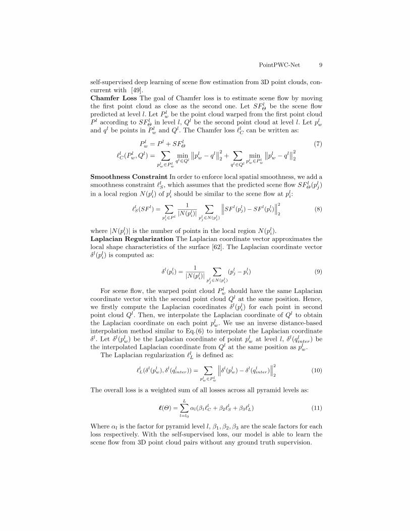
self-supervised deep learning of scene flow estimation from 3D point clouds, con-current with [49].Chamfer Loss The goal of Chamfer loss is to estimate scene flow by movingthe first point cloud as close as the second one. Let SF lΘ be the scene flowpredicted at level l. Let P lw be the point cloud warped from the first point cloudP l according to SF lΘ in level l, Ql be the second point cloud at level l. Let plwand ql be points in P lw and Ql. The Chamfer loss `lC can be written as:

P lw = P l + SF lΘ (7)

`lC(P lw, Ql) =

∑plw∈P l

w

minql∈Ql

∥∥plw − ql∥∥22 +∑ql∈Ql

minplw∈P l

w

∥∥plw − ql∥∥22Smoothness Constraint In order to enforce local spatial smoothness, we add asmoothness constraint `lS , which assumes that the predicted scene flow SF lΘ(plj)

in a local region N(pli) of pli should be similar to the scene flow at pli:

`lS(SF l) =∑

pli∈Pl

1

|N(pli)|∑

plj∈N(pli)

∥∥∥SF l(plj)− SF l(pli)∥∥∥22

(8)

where |N(pli)| is the number of points in the local region N(pli).Laplacian Regularization The Laplacian coordinate vector approximates thelocal shape characteristics of the surface [62]. The Laplacian coordinate vectorδl(pli) is computed as:

δl(pli) =1

|N(pli)|∑

plj∈N(pli)

(plj − pli) (9)

For scene flow, the warped point cloud P lw should have the same Laplaciancoordinate vector with the second point cloud Ql at the same position. Hence,we firstly compute the Laplacian coordinates δl(pli) for each point in secondpoint cloud Ql. Then, we interpolate the Laplacian coordinate of Ql to obtainthe Laplacian coordinate on each point plw. We use an inverse distance-basedinterpolation method similar to Eq.(6) to interpolate the Laplacian coordinateδl. Let δl(plw) be the Laplacian coordinate of point plw at level l, δl(qlinter) bethe interpolated Laplacian coordinate from Ql at the same position as plw.

The Laplacian regularization `lL is defined as:

`lL(δl(plw), δl(qlinter)) =∑

plw∈P lw

∥∥∥δl(plw)− δl(qlinter)∥∥∥22

(10)

The overall loss is a weighted sum of all losses across all pyramid levels as:

`(Θ) =

L∑l=l0

αl(β1`lC + β2`

lS + β3`

lL) (11)

Where αl is the factor for pyramid level l, β1, β2, β3 are the scale factors for eachloss respectively. With the self-supervised loss, our model is able to learn thescene flow from 3D point cloud pairs without any ground truth supervision.

10 W. Wu et al.

Table 1. Evaluation results on the FlyingThings3D and KITTI datasets.Self means self-supervised, Full means fully-supervised. All approaches are (at least)trained on FlyingThings3D. On KITTI, Self and Full refer to the respective modelstrained on FlyingThings3D that is directly evaluated on KITTI, while Self+Self meansthe model is firstly trained on FlyingThings3D with self-supervision, then fine-tunedon KITTI with self-supervision as well. Full+Self means the model is trained withfull supervision on FlyingThings3D, then fine-tuned on KITTI with self-supervision.ICP [5], FGR [85], and CPD [50] are traditional method that does not require training.Our model outperforms all baselines by a large margin on all metrics

Dataset Method Sup. EPE3D(m)↓ Acc3DS↑ Acc3DR↑ Outliers3D↓ EPE2D(px )↓ Acc2D↑

Flyingthings3D

ICP(rigid) [5] Self 0.4062 0.1614 0.3038 0.8796 23.2280 0.2913FGR(rigid) [85] Self 0.4016 0.1291 0.3461 0.8755 28.5165 0.3037CPD(non-rigid) [50] Self 0.4887 0.0538 0.1694 0.9063 26.2015 0.0966PointPWC-Net Self 0.1213 0.3239 0.6742 0.6878 6.5493 0.4756

FlowNet3D [36] Full 0.1136 0.4125 0.7706 0.6016 5.9740 0.5692SPLATFlowNet [63] Full 0.1205 0.4197 0.7180 0.6187 6.9759 0.5512original BCL [20] Full 0.1111 0.4279 0.7551 0.6054 6.3027 0.5669HPLFlowNet [20] Full 0.0804 0.6144 0.8555 0.4287 4.6723 0.6764PointPWC-Net Full 0.0588 0.7379 0.9276 0.3424 3.2390 0.7994

KITTI

ICP(rigid) [5] Self 0.5181 0.0669 0.1667 0.8712 27.6752 0.1056FGR(rigid) [85] Self 0.4835 0.1331 0.2851 0.7761 18.7464 0.2876CPD(non-rigid) [50] Self 0.4144 0.2058 0.4001 0.7146 27.0583 0.1980PointPWC-Net(w/o ft) Self 0.2549 0.2379 0.4957 0.6863 8.9439 0.3299PointPWC-Net(w/ ft) Self + Self 0.0461 0.7951 0.9538 0.2275 2.0417 0.8645

FlowNet3D [36] Full 0.1767 0.3738 0.6677 0.5271 7.2141 0.5093SPLATFlowNet [63] Full 0.1988 0.2174 0.5391 0.6575 8.2306 0.4189original BCL [20] Full 0.1729 0.2516 0.6011 0.6215 7.3476 0.4411HPLFlowNet [20] Full 0.1169 0.4783 0.7776 0.4103 4.8055 0.5938PointPWC-Net(w/o ft) Full 0.0694 0.7281 0.8884 0.2648 3.0062 0.7673PointPWC-Net(w/ ft) Full + Self 0.0430 0.8175 0.9680 0.2072 1.9022 0.8669

5 Experiments

In this section, we train and evaluate our PointPWC-Net on the FlyingThings3Ddataset [44] with the supervised loss and the self-supervised loss, respectively.Then, we evaluate the generalization ability of our model by first applying themodel on the real-world KITTI Scene Flow dataset [47, 46] without any fine-tuning. Then, with the proposed self-supervised losses, we further fine-tune ourpre-trained model on the KITTI dataset to study the best performance we couldobtain without supervision. Besides, we also compare the runtime of our modelwith previous work. Finally, we conduct ablation studies to analyze the contri-bution of each part of the model and the loss function.

Implementation Details. We build a 4-level feature pyramid from the inputpoint cloud. The weights α are set to be α0 = 0.02, α1 = 0.04, α2 = 0.08,and α3 = 0.16, with weight decay 0.0001.The scale factor β in self-supervisedlearning are set to be β1 = 1.0, β2 = 1.0, and β3 = 0.3. We train our modelstarting from a learning rate of 0.001 and reducing by half every 80 epochs. Allthe hyperparameters are set using the validation set of FlyingThings3D with8,192 points in each input point cloud.

PointPWC-Net 11

(a) PC1 and PC2 (b) GT

(d) CPD(non-rigid)

(c) FGR(rigid)

(e) PointPWC-Net(𝐹𝑢𝑙𝑙) (f) PointPWC-Net(𝑆𝑒𝑙𝑓)

Fig. 3. Results on the FlyingThings3D dataset. In (a), 2 point clouds PC1 andPC2 are presented in Magenta and Green, respectively. In (b-f), PC1 is warped toPC2 based on the (computed) scene flow. (b) shows the ground truth; (c) Results fromFGR(rigid) [85]; (d) Results from CPD(non-rigid) [50]; (e) Results from PointPWC-Net(Full); (f) Results from PointPWC-Net(Self ). Red ellipses indicate locations withsignificant non-rigid motion. Enlarge images for better view. (Best viewed in color)

Evaluation Metrics. For fair comparison, we adopt the evaluation metricsthat are used in [20]. Let SFΘ denote the predicted scene flow, and SFGT bethe ground truth scene flow. The evaluate metrics are computed as follows:• EPE3D(m): ‖SFΘ − SFGT ‖2 averaged over each point in meters.• Acc3DS : the percentage of points with EPE3D < 0.05m or relative error < 5%.• Acc3DR: the percentage of points with EPE3D < 0.1m or relative error < 10%.• Outliers3D : the percentage of points with EPE3D> 0.3m or relative error> 10%.• EPE2D(px): 2D end point error obtained by projecting point clouds back tothe image plane.• Acc2D : the percentage of points whose EPE2D < 3px or relative error < 5%.

5.1 Supervised Learning

First we conduct experiments with supervised loss. To our knowledge, there is nopublicly available large-scale real-world dataset that has scene flow ground truthfrom point clouds (The input to the KITTI scene flow benchmark is 2D), thus wetrain our PointPWC-Net on the synthetic Flyingthings3D dataset, following [20].Then, the pre-trained model is directly evaluated on KITTI Scene Flow 2015dataset without any fine-tuning.Train and Evaluate on FlyingThings3D. The FlyingThings3D trainingdataset includes 19,640 pairs of point clouds, and the evaluation dataset in-cludes 3,824 pairs of point clouds. Our model takes n = 8, 192 points in eachpoint cloud. We first train the model with 1

4 of the training set(4,910 pairs), andthen fine-tune it on the whole training set, to speed up training.

12 W. Wu et al.

Table 2. Model design. A learnable cost volume preforms much better than innerproduct cost volume used in PWC-Net [65]. Using our cost volume instead of theMLP+Maxpool used in FlowNet3D’s flow embedding layer improves performance by20.6%. Compared to no warping, the warping layer improves the performance by 40.2%

Component Status EPE3D(m)↓

Cost VolumePWC-Net [65] 0.0821

MLP+Maxpool(learnable) [36] 0.0741Ours(learnable) 0.0588

Warping Layerw/o 0.0984w 0.0588

Table 1 shows the quantitative evaluation results on the Flyingthings3Ddataset. Our method outperforms all the methods on all metrics by a large mar-gin. Comparing to SPLATFlowNet, original BCL, and HPLFlowNet, our methodavoids the preprocessing step of building a permutohedral lattice from the input.Besides, our method outperforms HPLFlowNet on EPE3D by 26 .9 %. And, weare the only method with EPE2D under 4px, which improves over HPLFlowNetby 30 .7 %. See Fig.3(e) for example results.Evaluate on KITTI w/o Fine-tune. To study the generalization ability of ourPointPWC-Net, we directly take the model trained using FlyingThings3D andevaluate it on KITTI Scene Flow 2015 [46, 47] without any fine-tuning. KITTIScene Flow 2015 consists of 200 training scenes and 200 test scenes. To evaluateour PointPWC-Net, we use ground truth labels and trace raw point clouds asso-ciated with the frames, following [36, 20]. Since no point clouds and ground truthare provided on test set, we evaluate on all 142 scenes in the training set withavailable point clouds. We remove ground points with height < 0.3m following[20] for fair comparison with previous methods.

From Table 1, our PointPWC-Net outperforms all the state-of-the-art meth-ods, which demonstrates the generalization ability of our model. For EPE3D, ourmodel is the only one below 10cm, which improves over HPLFlowNet by 40 .6 %.For Acc3DS, our method outperforms both FlowNet3D and HPLFlowNet by35 .4 % and 25 .0 % respectively. See Fig.4(e) for example results.

5.2 Self-supervised Learning

Acquiring or annotating dense scene flow from real-world 3D point clouds isvery expensive, so it would be interesting to evaluate the performance of ourself-supervised approach. We train our model using the same procedure as insupervised learning, i.e. first train the model with one quarter of the trainingdataset, then fine-tune with the whole training set. Table 1 gives the quanti-tative results on PointPWC-Net with self-supervised learning. We compare ourmethod with ICP(rigid) [5], FGR(rigid) [85] and CPD(non-rigid) [50]. Becausetraditional point registration methods are not trained with ground truth, we canview them as self/un-supervised methods.

PointPWC-Net 13

(a) PC1 and PC2 (b) GT

(d) CPD(non-rigid)

(c) FGR(rigid)

(e) PointPWC-Net(𝑤/𝑜 𝑓𝑡+ 𝐹𝑢𝑙𝑙) (f) PointPWC-Net(𝑤/ 𝑓𝑡+ 𝑆𝑒𝑙𝑓 + 𝑆𝑒𝑙𝑓)

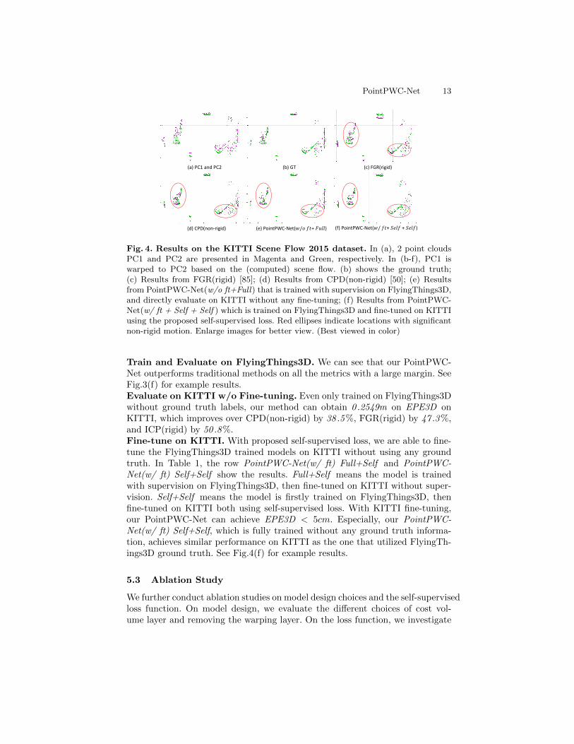
Fig. 4. Results on the KITTI Scene Flow 2015 dataset. In (a), 2 point cloudsPC1 and PC2 are presented in Magenta and Green, respectively. In (b-f), PC1 iswarped to PC2 based on the (computed) scene flow. (b) shows the ground truth;(c) Results from FGR(rigid) [85]; (d) Results from CPD(non-rigid) [50]; (e) Resultsfrom PointPWC-Net(w/o ft+Full) that is trained with supervision on FlyingThings3D,and directly evaluate on KITTI without any fine-tuning; (f) Results from PointPWC-Net(w/ ft + Self + Self ) which is trained on FlyingThings3D and fine-tuned on KITTIusing the proposed self-supervised loss. Red ellipses indicate locations with significantnon-rigid motion. Enlarge images for better view. (Best viewed in color)

Train and Evaluate on FlyingThings3D. We can see that our PointPWC-Net outperforms traditional methods on all the metrics with a large margin. SeeFig.3(f) for example results.Evaluate on KITTI w/o Fine-tuning. Even only trained on FlyingThings3Dwithout ground truth labels, our method can obtain 0 .2549m on EPE3D onKITTI, which improves over CPD(non-rigid) by 38 .5 %, FGR(rigid) by 47 .3 %,and ICP(rigid) by 50 .8 %.Fine-tune on KITTI. With proposed self-supervised loss, we are able to fine-tune the FlyingThings3D trained models on KITTI without using any groundtruth. In Table 1, the row PointPWC-Net(w/ ft) Full+Self and PointPWC-Net(w/ ft) Self+Self show the results. Full+Self means the model is trainedwith supervision on FlyingThings3D, then fine-tuned on KITTI without super-vision. Self+Self means the model is firstly trained on FlyingThings3D, thenfine-tuned on KITTI both using self-supervised loss. With KITTI fine-tuning,our PointPWC-Net can achieve EPE3D < 5cm. Especially, our PointPWC-Net(w/ ft) Self+Self, which is fully trained without any ground truth informa-tion, achieves similar performance on KITTI as the one that utilized FlyingTh-ings3D ground truth. See Fig.4(f) for example results.

5.3 Ablation Study

We further conduct ablation studies on model design choices and the self-supervisedloss function. On model design, we evaluate the different choices of cost vol-ume layer and removing the warping layer. On the loss function, we investigate

14 W. Wu et al.

Table 3. Loss functions. The Cham-fer loss is not enough to estimate a goodscene flow. With the smoothness con-straint, the scene flow result improves by38.2%. Laplacian regularization also im-proves slightly

Chamfer Smoothness Laplacian EPE3D(m)↓

X - - 0.2112X X - 0.1304X X X 0.1213

Table 4. Runtime. Average run-time(ms) on Flyingthings3D. The run-time for FlowNet3D and HPLFlowNet isreported from [20] on a single Titan V.The runtime for our PointPWC-Net is re-ported on a single 1080Ti

Method Runtime(ms)↓

FlowNet3D [36] 130.8HPLFlowNet [20] 98.4PointPWC-Net 117.4

removing the smoothness constraint and Laplacian regularization in the self-supervised learning loss. All models in the ablation studies are trained usingFlyingThings3D, and tested on the FlyingThings3D evaluation dataset.

Tables 2, 3 show the results of the ablation studies. In Table 2 we can seethat our design of the cost volume obtains significantly better results than theinner product-based cost volume in PWC-Net [65] and FlowNet3D [36], andthe warping layer is crucial for performance. In Table 3, we see that both thesmoothness constraint and Laplacian regularization improve the performance inself-supervised learning. In Table 4, we report the runtime of our PointPWC-Net, which is comparable with other deep learning based methods and muchfaster than traditional ones.

6 Conclusion

To better estimate scene flow directly from 3D point clouds, we proposed a novellearnable cost volume layer along with some auxiliary layers to build a coarse-to-fine deep network, called PointPWC-Net. Because of the fact that real-worldground truth scene flow is hard to acquire, we introduce a loss function thattrain the PointPWC-Net without supervision. Experiments on the FlyingTh-ings3D and KITTI datasets demonstrates the effectiveness of our PointPWC-Net and the self-supervised loss function, obtaining state-of-the-art results thatoutperform prior work by a large margin.

Acknowledgement

Wenxuan Wu and Li Fuxin were partially supported by the National ScienceFoundation (NSF) under Project #1751402, USDA National Institute of Foodand Agriculture (USDA-NIFA) under Award 2019-67019-29462, as well as bythe Defense Advanced Research Projects Agency (DARPA) under Contract No.N66001-17-12-4030 and N66001-19-2-4035. Any opinions, findings and conclu-sions or recommendations expressed in this material are those of the author(s)and do not necessarily reflect the views of the funding agencies.

PointPWC-Net 15

References

1. Amberg, B., Romdhani, S., Vetter, T.: Optimal step nonrigid icp algorithms forsurface registration. In: 2007 IEEE Conference on Computer Vision and PatternRecognition. pp. 1–8. IEEE (2007)

2. Bai, L., Yang, X., Gao, H.: Nonrigid point set registration by preserving localconnectivity. IEEE transactions on cybernetics 48(3), 826–835 (2017)

3. Behl, A., Paschalidou, D., Donne, S., Geiger, A.: Pointflownet: Learning represen-tations for rigid motion estimation from point clouds. In: Proceedings of the IEEEConference on Computer Vision and Pattern Recognition. pp. 7962–7971 (2019)

4. Bergen, J.R., Anandan, P., Hanna, K.J., Hingorani, R.: Hierarchical model-basedmotion estimation. In: European conference on computer vision. pp. 237–252.Springer (1992)

5. Besl, P.J., McKay, N.D.: Method for registration of 3-d shapes. In: Sensor fusionIV: control paradigms and data structures. vol. 1611, pp. 586–606. InternationalSociety for Optics and Photonics (1992)

6. Brown, B.J., Rusinkiewicz, S.: Global non-rigid alignment of 3-d scans. In: ACMSIGGRAPH 2007 papers, pp. 21–es (2007)

7. Brox, T., Bruhn, A., Papenberg, N., Weickert, J.: High accuracy optical flow esti-mation based on a theory for warping. In: European conference on computer vision.pp. 25–36. Springer (2004)

8. Bruhn, A., Weickert, J., Schnorr, C.: Lucas/kanade meets horn/schunck: Combin-ing local and global optic flow methods. International journal of computer vision61(3), 211–231 (2005)

9. Chabra, R., Straub, J., Sweeney, C., Newcombe, R., Fuchs, H.: Stereodrnet: Dilatedresidual stereonet. In: Proceedings of the IEEE Conference on Computer Visionand Pattern Recognition. pp. 11786–11795 (2019)

10. Choi, S., Zhou, Q.Y., Koltun, V.: Robust reconstruction of indoor scenes. In: Pro-ceedings of the IEEE Conference on Computer Vision and Pattern Recognition.pp. 5556–5565 (2015)

11. Danelljan, M., Meneghetti, G., Shahbaz Khan, F., Felsberg, M.: A probabilisticframework for color-based point set registration. In: Proceedings of the IEEE Con-ference on Computer Vision and Pattern Recognition. pp. 1818–1826 (2016)

12. Dewan, A., Caselitz, T., Tipaldi, G.D., Burgard, W.: Rigid scene flow for 3d li-dar scans. In: 2016 IEEE/RSJ International Conference on Intelligent Robots andSystems (IROS). pp. 1765–1770. IEEE (2016)

13. Dosovitskiy, A., Fischer, P., Ilg, E., Hausser, P., Hazirbas, C., Golkov, V., VanDer Smagt, P., Cremers, D., Brox, T.: Flownet: Learning optical flow with convolu-tional networks. In: Proceedings of the IEEE international conference on computervision. pp. 2758–2766 (2015)

14. Fan, H., Su, H., Guibas, L.J.: A point set generation network for 3d object recon-struction from a single image. In: Proceedings of the IEEE conference on computervision and pattern recognition. pp. 605–613 (2017)

15. Fu, M., Zhou, W.: Non-rigid point set registration via mixture of asymmetric gaus-sians with integrated local structures. In: 2016 IEEE International Conference onRobotics and Biomimetics (ROBIO). pp. 999–1004. IEEE (2016)

16. Ge, S., Fan, G.: Non-rigid articulated point set registration with local structurepreservation. In: Proceedings of the IEEE Conference on Computer Vision andPattern Recognition Workshops. pp. 126–133 (2015)

16 W. Wu et al.

17. Ge, S., Fan, G., Ding, M.: Non-rigid point set registration with global-local topol-ogy preservation. In: Proceedings of the IEEE Conference on Computer Vision andPattern Recognition Workshops. pp. 245–251 (2014)

18. Gelfand, N., Mitra, N.J., Guibas, L.J., Pottmann, H.: Robust global registration.In: Symposium on geometry processing. vol. 2, p. 5. Vienna, Austria (2005)

19. Groh, F., Wieschollek, P., Lensch, H.P.: Flex-convolution. In: Asian Conference onComputer Vision. pp. 105–122. Springer (2018)

20. Gu, X., Wang, Y., Wu, C., Lee, Y.J., Wang, P.: Hplflownet: Hierarchical permu-tohedral lattice flownet for scene flow estimation on large-scale point clouds. In:Proceedings of the IEEE Conference on Computer Vision and Pattern Recognition.pp. 3254–3263 (2019)

21. Guo, Y., Bennamoun, M., Sohel, F., Lu, M., Wan, J.: 3d object recognition incluttered scenes with local surface features: a survey. IEEE Transactions on PatternAnalysis and Machine Intelligence 36(11), 2270–2287 (2014)

22. Hermosilla, P., Ritschel, T., Vazquez, P.P., Vinacua, A., Ropinski, T.: Monte carloconvolution for learning on non-uniformly sampled point clouds. In: SIGGRAPHAsia 2018 Technical Papers. p. 235. ACM (2018)

23. Holz, D., Ichim, A.E., Tombari, F., Rusu, R.B., Behnke, S.: Registration with thepoint cloud library: A modular framework for aligning in 3-d. IEEE Robotics &Automation Magazine 22(4), 110–124 (2015)

24. Horn, B.K., Schunck, B.G.: Determining optical flow. Artificial intelligence 17(1-3),185–203 (1981)

25. Hua, B.S., Tran, M.K., Yeung, S.K.: Pointwise convolutional neural networks. In:Proceedings of the IEEE Conference on Computer Vision and Pattern Recognition.pp. 984–993 (2018)

26. Huguet, F., Devernay, F.: A variational method for scene flow estimation fromstereo sequences. In: 2007 IEEE 11th International Conference on Computer Vi-sion. pp. 1–7. IEEE (2007)

27. Hur, J., Roth, S.: Self-supervised monocular scene flow estimation. In: Proceedingsof the IEEE/CVF Conference on Computer Vision and Pattern Recognition. pp.7396–7405 (2020)

28. Ilg, E., Mayer, N., Saikia, T., Keuper, M., Dosovitskiy, A., Brox, T.: Flownet2.0: Evolution of optical flow estimation with deep networks. In: Proceedings ofthe IEEE conference on computer vision and pattern recognition. pp. 2462–2470(2017)

29. Jain, V., Zhang, H., van Kaick, O.: Non-rigid spectral correspondence of trianglemeshes. International Journal of Shape Modeling 13(01), 101–124 (2007)

30. Jia, X., De Brabandere, B., Tuytelaars, T., Gool, L.V.: Dynamic filter networks.In: Advances in Neural Information Processing Systems. pp. 667–675 (2016)

31. Kendall, A., Martirosyan, H., Dasgupta, S., Henry, P., Kennedy, R., Bachrach, A.,Bry, A.: End-to-end learning of geometry and context for deep stereo regression.In: Proceedings of the IEEE International Conference on Computer Vision. pp.66–75 (2017)

32. Lee, M., Fowlkes, C.C.: Cemnet: Self-supervised learning for accurate continuousego-motion estimation. In: Proceedings of the IEEE Conference on Computer Vi-sion and Pattern Recognition Workshops. pp. 0–0 (2019)

33. Lei, H., Jiang, G., Quan, L.: Fast descriptors and correspondence propagation forrobust global point cloud registration. IEEE Transactions on Image Processing26(8), 3614–3623 (2017)

PointPWC-Net 17

34. Li, Y., Bu, R., Sun, M., Wu, W., Di, X., Chen, B.: Pointcnn: Convolution on x-transformed points. In: Advances in Neural Information Processing Systems. pp.820–830 (2018)

35. Liu, L., Zhai, G., Ye, W., Liu, Y.: Unsupervised learning of scene flow estimationfusing with local rigidity. In: Proceedings of the 28th International Joint Conferenceon Artificial Intelligence. pp. 876–882. AAAI Press (2019)

36. Liu, X., Qi, C.R., Guibas, L.J.: Flownet3d: Learning scene flow in 3d point clouds.In: Proceedings of the IEEE Conference on Computer Vision and Pattern Recog-nition. pp. 529–537 (2019)

37. Lu, M., Zhao, J., Guo, Y., Ma, Y.: Accelerated coherent point drift for automaticthree-dimensional point cloud registration. IEEE Geoscience and Remote SensingLetters 13(2), 162–166 (2015)

38. Ma, J., Chen, J., Ming, D., Tian, J.: A mixture model for robust point matchingunder multi-layer motion. PloS one 9(3) (2014)

39. Ma, J., Jiang, J., Zhou, H., Zhao, J., Guo, X.: Guided locality preserving featurematching for remote sensing image registration. IEEE transactions on geoscienceand remote sensing 56(8), 4435–4447 (2018)

40. Ma, J., Zhao, J., Jiang, J., Zhou, H.: Non-rigid point set registration with robusttransformation estimation under manifold regularization. In: Thirty-First AAAIConference on Artificial Intelligence (2017)

41. Ma, J., Zhao, J., Yuille, A.L.: Non-rigid point set registration by preserving globaland local structures. IEEE Transactions on image Processing 25(1), 53–64 (2015)

42. Ma, J., Zhou, H., Zhao, J., Gao, Y., Jiang, J., Tian, J.: Robust feature match-ing for remote sensing image registration via locally linear transforming. IEEETransactions on Geoscience and Remote Sensing 53(12), 6469–6481 (2015)

43. Makadia, A., Patterson, A., Daniilidis, K.: Fully automatic registration of 3d pointclouds. In: 2006 IEEE Computer Society Conference on Computer Vision andPattern Recognition (CVPR’06). vol. 1, pp. 1297–1304. IEEE (2006)

44. Mayer, N., Ilg, E., Hausser, P., Fischer, P., Cremers, D., Dosovitskiy, A., Brox,T.: A large dataset to train convolutional networks for disparity, optical flow, andscene flow estimation. In: Proceedings of the IEEE Conference on Computer Visionand Pattern Recognition. pp. 4040–4048 (2016)

45. Menze, M., Geiger, A.: Object scene flow for autonomous vehicles. In: Proceedingsof the IEEE Conference on Computer Vision and Pattern Recognition. pp. 3061–3070 (2015)

46. Menze, M., Heipke, C., Geiger, A.: Joint 3d estimation of vehicles and scene flow.In: ISPRS Workshop on Image Sequence Analysis (ISA) (2015)

47. Menze, M., Heipke, C., Geiger, A.: Object scene flow. ISPRS Journal of Pho-togrammetry and Remote Sensing (JPRS) (2018)

48. Mian, A.S., Bennamoun, M., Owens, R.: Three-dimensional model-based objectrecognition and segmentation in cluttered scenes. IEEE transactions on patternanalysis and machine intelligence 28(10), 1584–1601 (2006)

49. Mittal, H., Okorn, B., Held, D.: Just go with the flow: Self-supervised scene flowestimation. In: Proceedings of the IEEE/CVF Conference on Computer Vision andPattern Recognition. pp. 11177–11185 (2020)

50. Myronenko, A., Song, X.: Point set registration: Coherent point drift. IEEE trans-actions on pattern analysis and machine intelligence 32(12), 2262–2275 (2010)

51. Nguyen, T.M., Wu, Q.J.: Multiple kernel point set registration. IEEE transactionson medical imaging 35(6), 1381–1394 (2015)

52. Pomerleau, F., Colas, F., Siegwart, R., Magnenat, S.: Comparing icp variants onreal-world data sets. Autonomous Robots 34(3), 133–148 (2013)

18 W. Wu et al.

53. Qi, C.R., Su, H., Mo, K., Guibas, L.J.: Pointnet: Deep learning on point sets for3d classification and segmentation. In: Proceedings of the IEEE Conference onComputer Vision and Pattern Recognition. pp. 652–660 (2017)

54. Qi, C.R., Yi, L., Su, H., Guibas, L.J.: Pointnet++: Deep hierarchical feature learn-ing on point sets in a metric space. In: Advances in neural information processingsystems. pp. 5099–5108 (2017)

55. Qu, H.B., Wang, J.Q., Li, B., Yu, M.: Probabilistic model for robust affine andnon-rigid point set matching. IEEE transactions on pattern analysis and machineintelligence 39(2), 371–384 (2016)

56. Ranjan, A., Black, M.J.: Optical flow estimation using a spatial pyramid network.In: Proceedings of the IEEE Conference on Computer Vision and Pattern Recog-nition. pp. 4161–4170 (2017)

57. Ravanbakhsh, S., Schneider, J., Poczos, B.: Deep learning with sets and pointclouds. arXiv preprint arXiv:1611.04500 (2016)

58. Revaud, J., Weinzaepfel, P., Harchaoui, Z., Schmid, C.: Epicflow: Edge-preservinginterpolation of correspondences for optical flow. In: Proceedings of the IEEE con-ference on computer vision and pattern recognition. pp. 1164–1172 (2015)

59. Saval-Calvo, M., Azorin-Lopez, J., Fuster-Guillo, A., Villena-Martinez, V., Fisher,R.B.: 3d non-rigid registration using color: Color coherent point drift. ComputerVision and Image Understanding 169, 119–135 (2018)

60. Shin, J., Triebel, R., Siegwart, R.: Unsupervised discovery of repetitive objects. In:2010 IEEE International Conference on Robotics and Automation. pp. 5041–5046.IEEE (2010)

61. Simonovsky, M., Komodakis, N.: Dynamic edge-conditioned filters in convolutionalneural networks on graphs. In: Proceedings of the IEEE conference on computervision and pattern recognition. pp. 3693–3702 (2017)

62. Sorkine, O.: Laplacian mesh processing. In: Eurographics (STARs). pp. 53–70(2005)

63. Su, H., Jampani, V., Sun, D., Maji, S., Kalogerakis, E., Yang, M.H., Kautz, J.:Splatnet: Sparse lattice networks for point cloud processing. In: Proceedings of theIEEE Conference on Computer Vision and Pattern Recognition. pp. 2530–2539(2018)

64. Sun, D., Roth, S., Black, M.J.: A quantitative analysis of current practices inoptical flow estimation and the principles behind them. International Journal ofComputer Vision 106(2), 115–137 (2014)

65. Sun, D., Yang, X., Liu, M.Y., Kautz, J.: Pwc-net: Cnns for optical flow usingpyramid, warping, and cost volume. In: Proceedings of the IEEE Conference onComputer Vision and Pattern Recognition. pp. 8934–8943 (2018)

66. Tam, G.K., Cheng, Z.Q., Lai, Y.K., Langbein, F.C., Liu, Y., Marshall, D., Martin,R.R., Sun, X.F., Rosin, P.L.: Registration of 3d point clouds and meshes: A surveyfrom rigid to nonrigid. IEEE transactions on visualization and computer graphics19(7), 1199–1217 (2012)

67. Tao, W., Sun, K.: Asymmetrical gauss mixture models for point sets matching. In:Proceedings of the IEEE Conference on Computer Vision and Pattern Recognition.pp. 1598–1605 (2014)

68. Tatarchenko, M., Park, J., Koltun, V., Zhou, Q.Y.: Tangent convolutions for denseprediction in 3d. In: Proceedings of the IEEE Conference on Computer Vision andPattern Recognition. pp. 3887–3896 (2018)

69. Theiler, P.W., Wegner, J.D., Schindler, K.: Globally consistent registration of ter-restrial laser scans via graph optimization. ISPRS Journal of Photogrammetry andRemote Sensing 109, 126–138 (2015)

PointPWC-Net 19

70. Ushani, A.K., Eustice, R.M.: Feature learning for scene flow estimation from lidar.In: Conference on Robot Learning. pp. 283–292 (2018)

71. Ushani, A.K., Wolcott, R.W., Walls, J.M., Eustice, R.M.: A learning approach forreal-time temporal scene flow estimation from lidar data. In: 2017 IEEE Inter-national Conference on Robotics and Automation (ICRA). pp. 5666–5673. IEEE(2017)

72. Vedula, S., Baker, S., Rander, P., Collins, R., Kanade, T.: Three-dimensional sceneflow. In: Proceedings of the Seventh IEEE International Conference on ComputerVision. vol. 2, pp. 722–729. IEEE (1999)

73. Verma, N., Boyer, E., Verbeek, J.: Feastnet: Feature-steered graph convolutions for3d shape analysis. In: Proceedings of the IEEE Conference on Computer Visionand Pattern Recognition. pp. 2598–2606 (2018)

74. Vogel, C., Schindler, K., Roth, S.: Piecewise rigid scene flow. In: Proceedings ofthe IEEE International Conference on Computer Vision. pp. 1377–1384 (2013)

75. Vogel, C., Schindler, K., Roth, S.: 3d scene flow estimation with a piecewise rigidscene model. International Journal of Computer Vision 115(1), 1–28 (2015)

76. Wang, G., Chen, Y.: Fuzzy correspondences guided gaussian mixture model forpoint set registration. Knowledge-Based Systems 136, 200–209 (2017)

77. Wang, N., Zhang, Y., Li, Z., Fu, Y., Liu, W., Jiang, Y.G.: Pixel2mesh: Gener-ating 3d mesh models from single rgb images. In: Proceedings of the EuropeanConference on Computer Vision (ECCV). pp. 52–67 (2018)

78. Wang, S., Suo, S., Ma, W.C., Pokrovsky, A., Urtasun, R.: Deep parametric con-tinuous convolutional neural networks. In: Proceedings of the IEEE Conference onComputer Vision and Pattern Recognition. pp. 2589–2597 (2018)

79. Wang, Y., Sun, Y., Liu, Z., Sarma, S.E., Bronstein, M.M., Solomon, J.M.: Dynamicgraph cnn for learning on point clouds. ACM Transactions on Graphics (TOG)38(5), 146 (2019)

80. Wu, W., Qi, Z., Fuxin, L.: Pointconv: Deep convolutional networks on 3d pointclouds. In: Proceedings of the IEEE Conference on Computer Vision and PatternRecognition. pp. 9621–9630 (2019)

81. Xu, J., Ranftl, R., Koltun, V.: Accurate optical flow via direct cost volume pro-cessing. In: Proceedings of the IEEE Conference on Computer Vision and PatternRecognition. pp. 1289–1297 (2017)

82. Yin, Z., Shi, J.: Geonet: Unsupervised learning of dense depth, optical flow andcamera pose. In: Proceedings of the IEEE Conference on Computer Vision andPattern Recognition. pp. 1983–1992 (2018)

83. Yu, D., Yang, F., Yang, C., Leng, C., Cao, J., Wang, Y., Tian, J.: Fast rotation-freefeature-based image registration using improved n-sift and gmm-based parallel op-timization. IEEE Transactions on Biomedical Engineering 63(8), 1653–1664 (2015)

84. Zhang, S., Yang, K., Yang, Y., Luo, Y., Wei, Z.: Non-rigid point set registrationusing dual-feature finite mixture model and global-local structural preservation.Pattern Recognition 80, 183–195 (2018)

85. Zhou, Q.Y., Park, J., Koltun, V.: Fast global registration. In: European Conferenceon Computer Vision. pp. 766–782. Springer (2016)

86. Zhou, Z., Zheng, J., Dai, Y., Zhou, Z., Chen, S.: Robust non-rigid point set regis-tration using student’s-t mixture model. PloS one 9(3) (2014)

87. Zou, Y., Luo, Z., Huang, J.B.: Df-net: Unsupervised joint learning of depth andflow using cross-task consistency. In: Proceedings of the European Conference onComputer Vision (ECCV). pp. 36–53 (2018)