PNNL-27712

Interim Analysis of the EPRI CASS Round Robin Study November 2018

RE Jacob TL Moran AE Holmes AA Diaz MS Prowant

PNNL-27712

Interim Analysis of the EPRI CASS Round Robin Study RE Jacob TL Moran AE Holmes AA Diaz MS Prowant November 2018 Prepared for U.S. Nuclear Regulatory Commission under a Related Services Agreement with the U.S. Department of Energy Contract DE-AC05-76RL01830 Pacific Northwest National Laboratory Richland, Washington 99352

PNNL-27712

iii

Acknowledgments

The work described in this technical letter report was sponsored by the U.S. Nuclear Regulatory Commission (NRC), Office of Nuclear Regulatory Research (RES). The authors gratefully acknowledge the guidance and technical insights provided by Contracting Officer Representative (COR) Ms. Carol Nove (RES) and deputy COR Mr. Bruce Lin (RES) during the development of this report. In addition, within the Office of Nuclear Reactor Regulation, Pacific Northwest National Laboratory (PNNL) would like to thank Dr. David Alley and Dr. Stephen Cumblidge for their participation and contributions in support of past presentations, discussions, and engagements with industry staff that fed into the development of this document.

PNNL would like to thank staff at the Electric Power Research Institute (EPRI) NDE Center in Charlotte, North Carolina, for the opportunity to participate in the cast austenitic stainless steel (CASS) round robin (RR) exercise. PNNL appreciates the open dialogue and subsequent technical discussions over the past several months as both organizations have assessed the results of this study. In particular, PNNL would like to thank Mr. Doug Kull, Mr. Carl Latiolais, and Mr. Greg Selby of EPRI. Additionally, PNNL would like to thank Mr. Kevin Hacker of Dominion Energy for his support of cooperative discussions between EPRI, the NRC, and PNNL throughout the RR assessment process. PNNL also appreciates the 3D laser profiling work of Mr. James Watson and Mr. Mathew Holling of Creative Dezign Concepts in Moorsville, North Carolina.

The authors also wish to acknowledge Mr. Pat Heasler (PNNL – retired) as the original principal investigator for statistical RR analyses on CASS examinations at PNNL and thank him for his continued guidance and insights to the PNNL Technical Team. PNNL also recognizes Ms. Susan Crawford (PNNL – retired) for her direct role in leading the PNNL Team at the EPRI NDE Center during the course of the RR exercise and the assistance of Mr. Samuel Sexton (PNNL – intern) in analyzing some of the data. The PNNL Team gratefully acknowledges Ms. Kay Hass for her invaluable assistance in the technical editing and formatting of this report, and finally, the authors wish to recognize and thank Ms. Lori Bisping for her outstanding level of support and attention to detail as the lead administrator and project coordinator.

PNNL-27712

iv

Abbreviations and Acronyms

ADAMS Agencywide Documents Access and Management System ASME American Society of Mechanical Engineers CASS cast austenitic stainless steel COD crack opening displacement DMW dissimilar metal weldment EPRI Electric Power Research Institute FCP false call probability FCR false call rate ID inner diameter ISI inservice inspection LR letter report MOU Memorandum of Understanding NDA non-disclosure agreement NDE nondestructive examination NRC U.S. Nuclear Regulatory Commission PA phased array PARENT Program to Assess the Reliability of Emerging Nondestructive

Techniques PDI performance demonstration initiative PINC Program for the Inspection of Nickel Alloy Components PISC Programme for the Inspection of Steel Components PNNL Pacific Northwest National Laboratory POD probability of detection ROC receiver operating characteristic RR round robin RRS round robin study SNR signal-to-noise ratio TF thermal fatigue TLR technical letter report UT ultrasonic testing

PNNL-27712

v

Contents

Acknowledgments ...................................................................................................................... iii Abbreviations and Acronyms ...................................................................................................... iv 1.0 Background ......................................................................................................................... 1 2.0 Introduction .......................................................................................................................... 3 3.0 PNNL Data Analysis ............................................................................................................ 4

3.1 Grading Criteria ............................................................................................................ 4 3.2 Comparison of PNNL and EPRI Grading Criteria ......................................................... 8 3.3 Statistical Analysis ....................................................................................................... 8

4.0 Results .............................................................................................................................. 10 4.1 Detection Rate and FCP ............................................................................................ 10 4.2 Practice and Probe Frequency ................................................................................... 13 4.3 Weld Crowns and Detection Angle ............................................................................. 16 4.4 Flaw Types ................................................................................................................. 16

5.0 Explanation of Key Differences Between PNNL and EPRI ................................................. 18 5.1 Detection Rates .......................................................................................................... 18 5.2 False Call Probability .................................................................................................. 19

6.0 An Alternative Approach Using Defined Grading Units ...................................................... 22 7.0 POD Curves ...................................................................................................................... 25 8.0 Discussion and Conclusions .............................................................................................. 29 9.0 References ........................................................................................................................ 33

PNNL-27712

vi

Figures

Figure 1. Flowchart Used for Grading Reported Flaws ............................................................ 7 Figure 2. PNNL Detection Rates ........................................................................................... 10 Figure 3. PNNL False Call Probability ................................................................................... 11 Figure 4. ROC Plot for All Participants .................................................................................. 12 Figure 5. PNNL Detection Rates for Each Team and Each Specimen Group ........................ 12 Figure 6. PNNL Detection Rates for Team Groups by Specimen Size .................................. 14 Figure 7. ROC Plots for All Participants by Specimen Size ................................................... 15 Figure 8. An Example of Two Different Crack Types ............................................................. 17 Figure 9. Detection Rates for Different Flaw Types ............................................................... 17 Figure 10. Detection Rate in a Subset of Specimens .............................................................. 18 Figure 11. Hypothetical Example of Grading Units .................................................................. 20 Figure 12. Detection Rates with Alternative Grading Units ...................................................... 24 Figure 13. False Call Probabilities with Alternative Grading Units ........................................... 24 Figure 14. Comparison of POD Curves With and Without FCP ............................................... 26 Figure 15. POD Curves for Each Team for the Three Grading Approaches ............................ 27 Figure 16. POD in 36” Specimens for Team Groups ............................................................... 28

Tables

Table 1. Hypothetical Example of Grading Units .................................................................. 20

PNNL-27712

1

1.0 Background

Pacific Northwest National Laboratory (PNNL) has been performing nondestructive examination (NDE) research under the sponsorship and guidance of the U.S. Nuclear Regulatory Commission (NRC) Office of Research since the 1970s. A primary objective of the research at PNNL has been to assess the effectiveness and reliability of advanced NDE methods for inservice inspection (ISI) of light-water reactor components. Within this body of work, a specific task has been created that focuses on developing and evaluating state-of-the-art technical approaches for inspecting nuclear reactor components that pose significant challenges to ultrasonic testing (UT) inspection methods used by the commercial nuclear power industry. In particular, some of this work has been focused on assessing the capabilities of advanced NDE methods for application on cast austenitic stainless steel (CASS) materials. CASS piping components are fabricated using static or centrifugal casting techniques, yielding coarse-grained, anisotropic microstructures that are challenging to examine.

A cooperative effort between the NRC and the Electric Power Research Institute (EPRI) was defined under Task 6 of the Addendum to the Memorandum of Understanding (MOU) between the NRC and EPRI on Cooperative Nuclear Safety Research – Nondestructive Examination, Attachment 2 Cast Austenitic Stainless Steel. Details associated with the MOU Addendum and the CASS cooperative work can be found in the Agencywide Documents Access and Management System (ADAMS) (Weber and Wilmshurst 2017).

Under the MOU, PNNL participated in a CASS round robin study (RRS) conducted by EPRI. EPRI’s primary aim for the CASS RRS was to “evaluate the detection performance of modern NDE equipment and techniques” for the examination of flaws in CASS components to guide development of future American Society of Mechanical Engineers (ASME) Section XI, Appendix VIII, Supplement 9 requirements (EPRI 2018). The RRS provided an excellent opportunity to demonstrate and assess the capabilities of advanced low-frequency phased array (PA)-UT methods for flaw detection in CASS. Domestic and international organizations were invited to participate in this RRS, including research laboratories and equipment vendors. Although PNNL offered their expertise in the planning and preparation stages of the RRS, PNNL’s involvement began in the spring of 2016 with their own inspection protocol development and other preparatory lab work. PNNL collected and analyzed data at the EPRI NDE Center as a blind study participant in August 2016. Following this, PNNL conducted an independent assessment of the entire RRS under the MOU. PNNL relied on their extensive knowledge of analyzing RR studies through their involvement in various domestic and international round robins, including the Programme for the Inspection of Steel Components (PISC) (Bates et al. 1987; Heasler et al. 1993), the Program to Assess the Reliability of Emerging Nondestructive Techniques (PARENT) (Meyer and Heasler 2017), and the Program for the Inspection of Nickel Alloy Components (PINC) (Cumblidge et al. 2010). In large part, the experiences and lessons learned from these RR assessments underpin the technical bases for how PNNL approached the analysis of the EPRI CASS RR data.

PNNL-27712

2

EPRI requested that all information associated with the CASS RRS, including data, mockup configurations, and flaw true-state1 information, be treated as secured, per an EPRI-developed security protocol. Therefore, PNNL participants, and a few additional PNNL analytical and NRC Staff were each required to sign a non-disclosure agreement (NDA) until such time that the RRS is completed and EPRI releases this information. It should be noted that EPRI stated in their RRS protocol2 that “the examination organization will be provided the test data as well as the specimen information so that it may be used at their discretion for training or other purposes.” As of the publication of this interim letter report, this has not yet occurred. In the meantime, the NRC has requested that PNNL document their independent and objective results, conclusions, and key observations of PNNL’s participation and subsequent statistical analyses in a non-secured, open document accessible by both NRC Staff and the general public. This interim report is intended to provide this information within the security guidelines of the NDA. PNNL is developing and will deliver to the NRC in late 2018 a technical letter report (TLR) that includes all relevant details associated with the RRS. However, this report will not be made publicly available until EPRI releases the specimen information.

1 Actual “true-states” for cracks used in round robin studies are generally determined by destructive analysis after-the-fact. However, for purposes of maintaining the integrity of the specimens and the data analyses reported in this document, flaw information supplied by EPRI such as location, orientation, length, and through-wall depth will be considered factual. 2 “Cast Austenitic Stainless Steel Non Destructive Evaluation Protocol for Conducting Blind Round-Robin Study.” Doug Kull and Carl Latiolais, March 30, 2015. Non-public document.

PNNL-27712

3

2.0 Introduction

PNNL was tasked to provide the NRC with an independent assessment of all aspects of the CASS RRS, including the mockups, the project execution and outcomes, analytical results, and technical reports published by EPRI. PNNL’s analysis focused on determining the probability of detection (POD) and the false call probability (FCP) of all RRS participants’ data. PNNL assessed overall flaw distribution, locations, and dimensions, and evaluated, based on previous experience and input from industry sources, whether the mockups were representative of actual CASS piping field conditions. PNNL assessed the execution of the RRS to determine what, if any, confounding variables may have contributed to complications in EPRI’s or PNNL’s analysis.

EPRI and PNNL took different approaches to the RRS data analysis, with each organization applying their unique perspective to the data analysis: PNNL relied on their experience with previous round robin studies, while EPRI approached the RRS analysis from a performance demonstration initiative (PDI) perspective. In doing so, EPRI concentrated their analysis more on flaw characterization (length- and depth-sizing), and PNNL’s focus was on detectability of flaw signals in the presence of multiple coherent responses.

As of this writing, EPRI continues to maintain the security of the specimens, including information about specific specimen configurations and flaws. Therefore, the focus of this interim report is limited to the dissemination of the results of PNNL’s independent analysis of the RRS data. Included is an explanation of the discrepancies between PNNL’s results and EPRI’s published analysis. Furthermore, all identifying information about specimens or flaws has been withheld, but will be presented in the forthcoming TLR. In addition, descriptions of PNNL’s preparatory work, data acquisition protocols, and data analysis methods have been omitted for brevity; this detailed information will also be included in the forthcoming TLR. Note that EPRI provided a general description of the RR specimens in their report, so additional specimen descriptions will not be given here. Finally, all participants’ identities have been anonymized so that specific data cannot be paired to a participating organization.

Revision 1 of the EPRI report is publicly available (EPRI 2018). Note that throughout this report, all mentions of EPRI’s results and/or analysis refer to that report and this reference will not be noted repeatedly.

PNNL-27712

4

3.0 PNNL Data Analysis

Twenty specimens were fabricated for the RRS, plus a few additional practice specimens. The specimens were circumferentially welded pipe segments with three different configurations identified by the nominal outside diameter: 12 in. (31 cm), 28 in. (71 cm), and 36 in. (91 cm), hereafter referred to as 12”, 28”, and 36”, respectively. These specimens were similar in size and configuration to those found in Combustion Engineering and Westinghouse pressurized water reactors. Many of the specimens had geometrical features added to them. As EPRI stated in their report, some mockups “were designed to include weld crowns as a scan access obstruction.” Several of the mockups were “designed to contain a counterbore adjacent to the weld region,” including “intermittent counterbore.” Finally, some mockups were “designed to contain varying degrees of root condition,” including convex root, concave root, or no root.

After PNNL’s blind participation in the RR (data collection and analysis), EPRI provided PNNL with specimen true-state information, including flaw circumferential start/stop positions, flaw axial locations, flaw types, and start/stop positions of other geometrical conditions (e.g., convex/concave root conditions and counterbore). PNNL was allowed to retain copies of their own UT scan image files and data analyses, but PNNL did not receive any other participants’ scans or calls. During a subsequent visit to EPRI, PNNL acquired photographs and 3D laser profiles of the specimen inner diameter (ID) surfaces and measured the weld crowns with contour gauges. After publication of Revision 0 of EPRI’s technical report in September 2017, PNNL received the other participants’ flaw call data (including reported flaw start/stop positions and axial locations), specific information about the participants’ probe frequencies, and the sizes and locations of the grading units used by EPRI in their analysis. PNNL was not provided any identifying information about team aliases applied by EPRI to participants’ data.

3.1 Grading Criteria

The grading criteria—the criteria used to determine whether a reported flaw counts as a detection or a false call—are key to the analysis and interpretation of the RRS data. PNNL recognized early on that the outcome of the RRS would be shaped almost wholly by the grading criteria. Therefore, it was PNNL’s initial goal to develop grading criteria that could provide an objective account of flaw detection that would accurately represent the intentions of the participating teams and provide insights into the capabilities of currently available UT methods and equipment. This required the use of both sound engineering judgment and a method of objectively distinguishing between reported flaws that were calls of actual flaws, calls of geometrical conditions, and false calls. In a subsequent analysis, different grading criteria were implemented in an effort to examine the effects of approaching the data analysis in a more conventional way; Section 6.0 describes this alternative approach.

PNNL developed grading criteria after they had received and thoroughly reviewed all of the participants’ reported flaw data in light of the true-state flaw and geometry information. PNNL looked for patterns in reported flaws of individual teams, as well as all teams as a whole population, while considering the spatial relationships between reported flaws and the intended, or true, flaws and geometrical conditions. Note that participants were not asked to identify geometrical conditions, but many reported flaws were clearly influenced by weld root or counterbore. Specific grading criteria were then developed, with justifications, to classify each reported flaw without relying on any interventions during grading. PNNL’s detection and grading

PNNL-27712

5

criteria are listed below along with brief justifications and descriptions of their intended purposes. For reference, the following terms are defined:

• reported flaw or reported call – an indication reported by a participating team

• true call – a reported flaw that correctly identifies an intended flaw

• geometrical feature call or geometry call – a reported flaw that identifies a geometrical feature, such as counterbore or weld root

• false call – a reported flaw that does not correctly identify an intended flaw or a geometrical feature (note that for PNNL’s analysis, geometrical feature calls were often grouped with false calls)

• no call or ignored call – a call that is considered as a non-detection and is therefore not included in the analysis

PNNL established the following guidelines before grading the data:

• Based on the grading criteria, each reported flaw may count as one (and only one) of the following—a true call, a geometrical feature call, a false call, or no call (ignored).

– For example, a single reported flaw cannot be counted as both a false call and a true call or as multiple false calls, regardless of the reported flaw length or how many different features (i.e., true flaws, weld root, counterbore, or unflawed material) that the reported flaw overlaps. This is to prevent an arbitrary assignment of unflawed grading units—and the subsequent subdivision of reported flaws—from artificially inflating the number of actual false calls. This approach emphasizes detection capability over examiner performance.

• There are no axial grading units.

– This is consistent with EPRI’s approach to indefinitely extend circumferential grading units in the axial direction. The data showed that many teams apparently reported signals from extraneous flaws or mode conversions. These reported flaws were generally in the correct circumferential position but varied axially from the true flaw position by as much as about 50 mm (2 in.). Because of the consistent and widespread nature of the problem among teams and specimens, no axial grading units were adopted.

• Flaws that do not fall within EPRI’s defined examination region are ignored. The examination region encompassed the weld region, extending from 6.4 mm (0.25 in.) axially beyond each counterbore, and only included the inner one-third volume of the specimen.

– This excluded a single flaw in one specimen. Because no teams reported the flaw, invoking this rule had little or no effect on the outcomes.

• There are no length criteria for reported flaws.

– This is a significant variation from EPRI’s detection criteria. EPRI implemented a rule that required reported flaws to be at least 50% of the length of the true flaw, otherwise the reported flaw was ignored. PNNL carefully examined the data and found, for example, that there were flaws that every team reported, yet virtually every team’s reported flaw was <50% of the true flaw length resulting in no credited detections. After considering this approach and examining the data, PNNL chose not to use length-based detection criteria. PNNL approached the RRS as an exercise about detection of flaws

PNNL-27712

6

and decided that length-sizing accuracy should be handled in a separate analysis. (Note that PNNL has not yet done an analysis of length-sizing accuracy.)

The process for grading is summarized in Figure 1. The specific rules for grading are as follows:

1. All reported flaws that are axial or primarily axial are ignored.

○ This is consistent with EPRI’s approach. Since not all teams attempted to detect axial flaws, EPRI and PNNL ignored all axial true flaws and axial reported flaws.

○ As a corollary to this, any circumferential (or primarily circumferential) reported flaws that overlap with an axial flaw are not considered true calls of the axial flaw.

2. To be counted as a true call, a reported flaw must overlap circumferentially, by any amount, with a true flaw. Similarly, to be counted as a geometry call, a reported flaw must overlap circumferentially, by any amount, with a geometrical feature.

○ This is consistent with EPRI’s second grading criterion.

○ After studying the data, it was concluded that a buffer, or tolerance, around the true flaws would not have had an impact on detection rates.

3. For cases where a reported flaw overlaps at least partially with a true flaw and a geometrical feature (i.e., weld root and/or counterbore), the reported flaw is assigned to be either a true call or geometrical feature call depending on which midpoint (flaw or geometry) is closest to that of the reported flaw.

○ It was common for one or more geometrical features, such as weld root and/or counterbore, to overlap circumferentially with at least one true flaw. This proximity rule was effective at correctly assigning the reported flaw to what was inferred to be the intention of the reporting team.

○ There were a few exceptions where these grading criteria apparently misclassified geometry calls as true calls. This primarily occurred in cases where the geometrical feature and the true flaw were not substantially different in length and/or axial location. However, no cases were observed where true calls were misclassified as geometry or false calls.

○ Reported flaws that were determined to be calls of geometrical features were categorized as geometry calls. For analysis purposes, geometry calls were counted first as no calls, then recategorized as false calls in order to help elucidate the confounding effects of geometry.

4. If multiple reported flaws meet the detection criteria for a single true flaw, the reported flaw with the longest circumferential overlap with the true flaw will be used and the other reported flaw(s) will be ignored.

○ If multiple reported flaws overlap a true flaw, then only one should count as a detection. With no axial grading units, the decision of which reported flaw to keep is somewhat arbitrary. PNNL’s philosophy was to keep the most conservative (i.e., longest) reported flaw.

○ EPRI had a similar criterion, except they used a proximity rule and kept the reported flaw that was closest axially to the true flaw. As with PNNL, one reported flaw was retained and the other(s) ignored.

PNNL-27712

7

5. Multiple false calls that overlap circumferentially (at least partially) become a single false call.

○ EPRI implemented a similar rule that if multiple reported flaws occupy the same unflawed grading unit, only one is counted.

○ PNNL observed only two cases where this rule was used after other grading criteria were applied. Geometry calls were exempt from this rule.

6. Any reported flaw that overlaps at least partially with more than one true flaw and has not been classified as a geometrical call is considered a false call.

○ This rule was intended to prevent indiscriminate reporting of long flaws simply to assure a detection. As it turned out, this rule was not required to be invoked.

○ EPRI implemented a maximum length criterion, which also served to prevent long reported flaws from counting as detections.

Figure 1. Flowchart Used for Grading Reported Flaws

PNNL-27712

8

3.2 Comparison of PNNL and EPRI Grading Criteria

PNNL grading criteria varied from those used by EPRI in three notable ways:

• The EPRI grading criteria used a length-based detection rule that discarded reported flaws that did not meet a minimum length threshold of at least 50% of the true flaw length, regardless of signal-to-noise (SNR) ratio or the number of teams that made similar calls. PNNL did not use any length-based grading criteria.

• PNNL’s grading criteria classified calls of geometrical features separately to allow for an analysis of the effects of geometry on teams’ FCP. Note that participating teams were not asked to identify geometry in their reported flaws.

• PNNL did not employ grading units; a false call was simply any reported flaw that did not meet the criteria of being assigned to a true flaw or a geometrical feature. EPRI implemented grading units, which resulted in a significantly different FCP than calculated by PNNL. Section 4.1 shows these results, and the discussion in Section 5.2 describes the reasons for the differences.

3.3 Statistical Analysis

The participating organizations collected and reported a total of seven data sets: two line scans and five raster scans. For this analysis, PNNL considered only the five raster scan data sets (EPRI Examiner Aliases A, B, C, E, and G). This was because PNNL had some concerns regarding the independence of two of the raster scan data sets and the two line-scan data sets (D and F). (These concerns were based on inferences made from EPRI’s report and not necessarily on any specific information given to PNNL.) Thus, the line scan data were ignored to avoid introducing potential bias into the analysis. In addition, PNNL’s analysis was single sided only (EPRI reported results of both a single-sided and a “simulated” dual-sided analysis), with upstream and downstream data treated as independent data sets, since they were acquired and analyzed separately. PNNL’s results will only be compared to EPRI’s single-sided analysis.

PNNL’s analysis primarily consisted of detection rate and FCP calculations for different scenarios. The detection rate (also referred to as the sensitivity) is the number of true detections divided by the total number of flaws. It is the POD and was calculated by Equation (1):

= =Number of True DetectionsDetection Rate POD

Number of Flaws (1)

In the absence of flawed grading units, a probability model was used to calculate FCP, as was done in PINC (Cumblidge et al. 2010). The FCP (the probability that a call intersects with an unflawed grading unit) was computed with Equation (2):

=Number of False CallsFCR

Total Length of Unflawed Grading Units (2a)

( )FCP 1 exp FCR guL= − − × (2b)

PNNL-27712

9

where FCR is the false call rate and Lgu is the average length of the unflawed grading unit. This equation assumes that the flaws are distributed randomly in the unflawed material. PNNL’s analysis showed that most of the false calls were not strictly random but were often associated with geometric features (see Section 4.1). Note that the FCP and FCR differ, because the FCR is calculated as a number of false calls per unit of length. Thus, FCR is not dependent on the grading unit size. FCP, on the other hand, is the probability that an inspector will report a flaw in an unflawed unit of material.3 To calculate FCP, the size of the unflawed grading units should, on average, be the same as that of the flawed grading units. With the average size of the flawed and unflawed grading units about the same, POD (or detection rate) and FCP are directly comparable, whereas POD and FCR are not.

PNNL calculated the detection rate for all teams together, individual teams, teams grouped by probe frequency, and teams grouped by whether they used practice specimens prior to acquiring data. PNNL also considered the detection rate for cases where data were separated by flaw type (EPRI described the flaw types as either laboratory-grown thermal fatigue cracks or simulated cracks). PNNL calculated the FCP for the teams as a group and for the individual teams. Geometry calls were first kept as a separate category, then they were combined with false calls to illustrate the effects of ID geometry on the FCP.

3 To facilitate comparison with EPRI’s results, it should be noted that EPRI’s false call rate is actually defined as a percentage; namely, the total number of unflawed grading units with candidate calls divided by the total number of unflawed grading units presented. This can equivalently be thought of as the probability that an unflawed grading unit has at least one candidate call. The PNNL FCP can also be thought of as the probability that a blank area of the same average size as the flawed grading units contains at least one false call, so they are essentially the same.

PNNL-27712

10

4.0 Results

4.1 Detection Rate and FCP

Figure 2 shows the results of PNNL’s detection rate calculations for each individual team (raster scans only) and for the teams as a group (note that EPRI’s group results included line scan data from Teams D and F). PNNL’s detection rates were consistently about 20 percentage points higher than those of EPRI. PNNL estimated that this equated to approximately 90 more true calls recorded by PNNL than by EPRI for the five teams. An explanation of this discrepancy is given in Section 5.1.

Figure 2. PNNL Detection Rates. The detection rate calculated by PNNL for each raster scan team and for the teams as a group. For comparison, EPRI’s published results are also shown.

The FCPs calculated by PNNL for each team and for the group are shown in Figure 3 (again, note that EPRI’s group results include Teams D and F). The results were broken down into false calls that did and did not include calls of geometrical features. Results show that the vast majority of reported false calls were attributable to geometrical features and were not caused by other factors such as the coarse grain structures of the CASS parent material. PNNL’s FCPs averaged about 12 percentage points lower than those reported by EPRI. PNNL estimated that this equated to a difference of about 85 false calls for the raster scans teams only. An explanation of this discrepancy is given in Section 5.2.

PNNL-27712

11

Figure 3. PNNL False Call Probability. The FCP was calculated by PNNL for each raster scan team and for the teams as a group. The chart shows the results of ignoring geometry calls and of counting them as false calls. For comparison, EPRI’s published results are also shown.

Figure 4 shows the receiver operating characteristic (ROC) plot (detection rate vs. FCP) for each raster scan team and for the group. Note that the large plot is an expanded view of the boxed region of the smaller plot. The diagonal line, or line of no discrimination, divides the ROC space into results that are better than random guessing (above the line) and worse than random (below the line). The green shaded region demarks the ≥80% detection rate and ≤20% FCP threshold that EPRI used as the benchmark of successful performance. PNNL’s results show that all teams had an FCP below the 20% threshold, even with geometry calls counted as false calls. Team G achieved a detection rate above the 80% threshold, and Team E was close behind at >75%. For comparison, EPRI’s reported results were included on the plot.

The detection rate was further broken down by team and specimen group (i.e., specimens grouped by piping diameter); see Figure 5. Team G achieved detection rates >80% for all specimen groups. Team E achieved >80% for the two larger specimen groups (28” and 36”), but not the 12” specimens. Interestingly, while Teams E and G achieved relative parity in detection rate between the 28” and 36” specimens, the other three teams did not. Indeed, Teams A, B, and C performed considerably better on the 36” specimens than on the 12” or 28” specimens. Reasons for this are unknown, but an array of variables, such as flaw types, flaw placement, ID geometries, weld crowns, and practice, may have contributed to this (several of these issues are discussed in this report, but many details have been omitted to maintain specimen security). Also of note are relatively poor performances by Teams A, B, and C in the 12” and 28” specimen groups, with detection rates at or below 50% in most cases.

PNNL-27712

12

Figure 4. ROC Plot for All Participants. The large graph is an expanded view of the boxed region of the smaller plot. The diagonal line is the line of no discrimination. Results of PNNL’s analysis with geometry calls ignored and included as false calls are shown. EPRI’s reported results are shown for comparison.

Figure 5. PNNL Detection Rates for Each Team and Each Specimen Group

PNNL-27712

13

4.2 Practice and Probe Frequency

There were two key differences between the approaches to the RRS by Teams A, B, and C (referred to as Group 1 for this discussion) and Teams E and G (Group 2)—the probe frequencies applied and the amount of practice. First, Group 1 used exclusively higher frequency probes (EPRI defined such “non-low-frequency” probes as ≥1 MHz), while Group 2 used higher frequency probes for the 12” specimens and “low frequency” probes (defined by EPRI as <1 MHz), or a combination of low- and high-frequency probes, for the larger specimens. Second, EPRI designed and fabricated a number of 12” and 28” practice specimens that were similar to those in the RRS. Note that teams were informed of the true-state of the practice specimens. All teams in Group 1 rejected the opportunity to practice on a 12” specimen, but both Group 2 teams did practice on a 12” specimen. All teams except Team C practiced on at least one 28” specimen. No teams were given opportunities to practice on a 36” specimen. In addition, at least one team was allowed the opportunity to practice with specimens at their own facility in advance of the actual RRS participation, while other teams practiced on-site upon arrival to participate in the RRS. Thus, opportunities for practice were not managed in a consistent manner. Note that the same teams that used higher frequency probes also practiced the least, so these two variables are unavoidably intertwined. Furthermore, it should be noted that the effects of practice were somewhat confounding for this analysis, since the effects of practice on human performance are difficult to quantify with such a small data set and other uncontrolled or unknown factors. Nevertheless, the data were used to provide some insight into the effects of practice and probe frequency on the detection rate.

To determine the effects of practice and probe frequency, detection rates were calculated for the two team groups; see Figure 6. The effects of practice are most evident in the 12” specimens, where all teams used higher frequency probes but Group 1 teams did not practice. The difference in detection rate between the two groups is significant. Not only is the detection rate for Group 2 nearly double that of Group 1, but the ROC plot for the 12” specimen in Figure 7 shows that the FCPs for Group 2 teams were about half those of the Group 1 teams. So, when all teams applied higher frequency probes in the small-bore specimens, teams that practiced had nearly double the detection rate and half the FCP.

The effects of frequency are most evident in the larger specimens. Figure 6 shows that the Group 2 teams that applied low-frequency probes on the larger specimens (28” and 36”) had higher detection rates than the Group 1 teams that used higher frequency probes. For the 28” specimen group, all teams were reported to have practiced except for Team C. Note in Figure 7 that the detection rate and FCP for Team C in the 28” specimen set are comparable to those for Teams A and B, indicating that differences in practice were likely not a significant factor in the 28” specimens for the Group 1 teams. Therefore, this wide discrepancy in detection rates in the 28” specimens between the two groups has been attributed to probe frequency. Also, no teams practiced on a 36” specimen, so the higher detection rate for Group 2 teams in the 36” specimens was attributed to applying lower probe frequencies.

PNNL-27712

14

Figure 6. PNNL Detection Rates for Team Groups by Specimen Size. Detection rates for Teams A, B, and C are compared to those of Teams E and G to illustrate the effects of practice and using low-frequency probes.

PNNL-27712

15

Figure 7. ROC Plots for All Participants by Specimen Size. The three plots show the PNNL-calculated detection rate vs. false call probability for each participant. Here, geometry calls were considered as false calls. The diagonal line is the line of no discrimination.

PNNL-27712

16

Results show that both practice and probe frequency played important roles in the outcome of the RRS, and both were confounding variables to the goal of determining the detection abilities of currently available technology for the examination of CASS. Practice could have been better controlled through an RRS protocol that required all teams to practice the same amount (or not at all). Probe frequency is more difficult to control because participating organizations were instructed to bring the inspection technology of their choice, even if it may not have been optimized for CASS examinations. In light of this, the effects of probe frequency could be better understood by increasing the number of participating teams. Unfortunately, this was out of EPRI’s control. Nevertheless, this RRS confirms previous PNNL work, which has shown that low-frequency PA probes are the best currently available technology for inspecting CASS (Anderson et al. 2007; Anderson et al. 2011; Diaz et al. 2012).

4.3 Weld Crowns and Detection Angle

The weld crowns on the 12” and 28” specimens may have played an important role in the RRS by limiting scan access across the weld. Consider the PNNL-calculated ROC plots for each specimen group shown in Figure 7 (the FCPs shown include geometry calls as false calls). All teams had >65% detection rate and ≤10% FCP in the 36” specimens, but the 12” and 28” specimens proved to be more challenging, especially for Teams A, B, and C. A factor to consider is that the 12” and 28” specimens had weld crowns that allowed scanning only up to the weld toe. The 36” specimens did not have weld crowns, and scanning was allowed up to the weld centerline. The presence of the impeding weld crowns meant that higher refraction angles were required for projected sound fields to reach the weld centerline and beyond in the 12” and 28” specimens. Because there were no weld crowns, lower refraction angles could be applied in the 36” specimens. It was determined that the average refraction angle used by the PNNL Team for detection in the 12” specimens was 56°, and in the 28” specimens was 54°, but in the 36” specimens was 40°. Because of the differences in material thickness, the metal paths in the 28” and 36” specimens were calculated to be about the same (3.4 in. and 3.5 in., respectively). However, for the probe matrices and frequencies applied, the PA sound beams would tend to focus less efficiently at higher angles resulting in larger spot sizes and lower peak sound field intensities (Anderson et al. 2011). It is unclear if or to what extent the presence of weld crowns may have affected some teams more than others (recall that practice and probe frequency remain confounding variables), but it is not surprising that the specimen groups with weld crowns had overall lower detection rates and higher FCPs.

4.4 Flaw Types

Detection rates were also calculated by team for the different flaw types. EPRI described the flaw types as “laboratory-grown” thermal fatigue (TF) cracks and “simulated” TF cracks. Figure 8 shows close-up photographs of examples of surface-breaking features of the two different types of cracks. The laboratory-grown TF cracks are observed to show branching, facets, and very tight crack opening displacements (CODs), especially at the ends, while the simulated TF cracks tended to be straighter, showed little or no branching, and had more consistent CODs along the entire length. Figure 9 shows the detection rate for each team for the different crack types. Most teams had more success detecting the laboratory-grown TF cracks than the simu-lated TF cracks, although Teams E and G—the teams that used low frequency and practiced the most—had more parity in their detection rates for the different crack types than the other

PNNL-27712

17

three teams. Additional details about these crack types and their placement within the speci-mens with respect to geometric conditions and the weld centerlines are omitted due to data security.

Figure 8. An Example of Two Different Crack Types. EPRI described the different crack types as “laboratory-grown” thermal fatigue (TF) cracks and “simulated cracks.” This figure shows an example of each (photos are not to scale).

Figure 9. Detection Rates for Different Flaw Types. The detection rates by team for the different flaw types, laboratory grown and simulated, are shown.

PNNL-27712

18

5.0 Explanation of Key Differences Between PNNL and EPRI

5.1 Detection Rates

As shown in Figure 2, there are significant differences in the detection rates calculated by PNNL and EPRI. To reconcile the differences, PNNL further analyzed the detection rates with and without the EPRI minimum length-based grading criterion (i.e., the criterion that reported flaws need to be at least 50% as long as the true flaw to count as a detection). Results are best illustrated by using a key subset of specimens in which the vast majority of the reported flaws that were too short to be counted as detected occurred (details about these specimens have been omitted due to data security). In this subset, PNNL counted 144 true flaw calls for all participating teams. After applying the EPRI minimum-length criterion, this was reduced to 64 true calls, a decrease of 80 reported flaws (approximately 56%). With the loss of 80 detections, the PNNL overall detection rate for this subset of specimens dropped from 76% to 34%. Figure 10 shows the PNNL detection rates for each raster scan team and select groups of teams with and without the minimum-length criterion applied for the specimen subset. The EPRI detection rate data for the same specimen subset are shown for comparison; these data are labeled “EPRI mean” and were calculated as closely as possible from data in the EPRI report. As shown in the figure, the PNNL results with the minimum-length criterion applied strongly agreed with the EPRI results (minor variances persisted due to other differences in grading criteria). The results therefore indicate that the length criterion implemented by EPRI was the primary difference between the PNNL and EPRI detection rates.

Figure 10. Detection Rate in a Subset of Specimens. This chart compares PNNL’s original detection rates with the detection rates obtained when the minimum length-based detection criterion was applied. Results are compared to EPRI’s detection rates to show that this criterion was the primary difference in detection rates between PNNL and EPRI.

PNNL-27712

19

Although PNNL did not calculate length root-mean-square error, it was clear from examining the data that length sizing was a significant challenge for all participating teams in many of the specimens. Whether a length-based criterion for detection in CASS is appropriate for a RR exercise can be debated. However, if the purpose of the RRS was to evaluate detection capabilities in CASS, then it is the opinion of PNNL that all reported detections should be considered. The consequences of counting all short calls as detections would then be manifest in length accuracy analyses instead of detection rates, and the results would likely reveal that accurate length sizing is a more significant challenge than was initially reported.

5.2 False Call Probability

This section describes the role that grading units played in the differences in false call assessments between PNNL and EPRI. A grading unit was defined as a region on a specimen that either contained a single intended flaw (flawed grading unit) or contained no intended flaws (unflawed grading unit). Recall that each specimen was scanned and graded independently from the upstream and downstream sides. There were several rules related to EPRI’s grading units: (1) the minimum grading unit size was 76 mm (3 in.); (2) at least a 25 mm (1 in.) buffer was required from each end of a flaw to the boundary of an adjacent unflawed grading unit; (3) each entire specimen was subdivided into grading units—there were no spaces or gaps between grading units; (4) only one true flaw was allowed per flawed grading unit (note that a true flaw must be wholly contained within a single flawed grading unit, but a geometrical feature could span multiple flawed and/or unflawed grading units); and (5) no more than one false call was counted per team per unflawed grading unit (i.e., multiple false calls by one team in one unflawed grading unit counted as one false call, even if the calls did not overlap circumferentially or were calls of different overlapping geometrical features).

After the specimens were subdivided into grading units, the EPRI grading criteria were applied. Figure 11 shows an example of how this was done. In this example,4 a true flaw is shown (blue) and three candidate calls are shown, one made from the upstream scan (green) and two from the downstream scan (red). The grey vertical lines represent the grading unit divisions, with the divisions labeled as UFGU or FGU for unflawed and flawed grading units, respectively. Any portion of a candidate call that was contained within an unflawed grading unit was counted as a separate false call. By applying this methodology, the three reported flaws would result in two true calls (one from each scan) and five false calls, one from the upstream scan (green arrow) and four from the downstream scan (red arrows), for a total of seven indications. For comparison, PNNL’s grading method would also have counted two true calls, one from each scan, but only one false call, from the downstream reported flaw located wholly outside the flawed grading unit. The results of this example are summarized in Table 1. EPRI noted in their report that, during a PDI examination, the invigilator can use discretion, presumably to not count as a false call a reported flaw that barely protrudes into an unflawed grading unit. However, they also note that the RRS grading was strictly objective so that the grading rules were applied equally to all participants. Thus, invigilator discretion was not used.

4 This example of applying grading units to the RRS data was based on an example provided to PNNL by EPRI to illustrate their methodology. Recall that upstream and downstream scans were treated as independent data sets.

PNNL-27712

20

Figure 11. Hypothetical Example of Grading Units. In this example, a hypothetical pipe section is shown with a flaw (blue), a call from the upstream (US) side (green), and two calls from the downstream (DS) side (red). One flawed grading unit (FGU1) and five unflawed grading units (UFGU1, UFGU2, etc.) are shown. The weld centerline (WCL) is illustrated as a dashed line. False calls tallied by EPRI’s method are indicated by arrows.

Table 1. Hypothetical Example of Grading Units. The results from Figure 11 are tallied in this table. From a total of three calls made (one US and two DS), PNNL would report three calls (two true and one false) while EPRI’s method would result in seven calls (two true and five false). Results illustrate how EPRI’s approach to determining false calls lead to a higher FCP.

The example in Figure 11 illustrates that this method of grading can result in considerably more false calls than the actual number of reported flaws. This methodology appears to have had a strong impact on the EPRI RRS analysis. For example, it was common for teams to mistake long geometrical features for flaws, resulting in reported flaws that typically spanned multiple unflawed grading units. Therefore, single reported flaws were commonly counted as multiple false calls. On the other hand, the number of true calls could never exceed the number of actual

PNNL-27712

21

reported flaws. As a result, the application of such grading units would not be expected to affect detection rates, but the increased number of false calls resulting from this approach did not realistically represent the performance of the participating teams. One way to avoid the problem of counting one reported flaw as multiple false calls is to space out the unflawed grading units (Heasler et al. 1993).

The average size of the unflawed grading units can also have a profound effect on the FCP (Heasler et al. 1990). Although it is not possible in every case, ideally all grading units—flawed and unflawed—should be approximately the same size in order to allow for comparison between detection statistics (Cumblidge et al. 2010; Heasler et al. 1993). However, the average size of EPRI unflawed grading units was about half that of the flawed grading units. To measure the consequences of this, PNNL increased the size of the unflawed grading units without affecting any adjacent flawed grading units in a subset of specimens where this was possible, then re-counted the number of false calls using the EPRI grading criteria. Results showed that when the average size of the unflawed grading units was increased to be on parity with that of the flawed grading units, the number of false calls dropped by 60, a 35% decrease.

Certain individual specimens disproportionately contributed to the overall number of false calls. To wit, two specimens of the 20 total led to about 125 EPRI false calls out of about 220 total. In other words, about 57% of the total number of false calls reported by EPRI were found in only 10% of the specimens. Even without subdividing reported flaws across unflawed grading units, PNNL counted 28% of false calls in the same specimens (counting geometry calls as false calls), which is still disproportionately high. The disproportionate number of false calls found in two specimens leads one to question whether these specimens are nominal or outliers with respect to field realism. PNNL concludes that these specimens are outliers and that data collected on these specimens should therefore be omitted from the RRS analysis.

In summary, three primary factors resulted in a much higher number of false calls measured by EPRI than by PNNL.

• One factor was the approach to counting false calls. A single reported flaw was often counted as multiple false calls—one false call for every unflawed grading unit it intersected with—which increased the total number of false calls. This issue was exacerbated when a team incorrectly reported as a flaw a geometrical feature that spanned multiple unflawed grading units.

• Another factor was the manner in which the unflawed grading units were defined. The unflawed grading units were, on average, half the size of the flawed grading units. This made it more likely for a given reported flaw to pass through multiple unflawed grading units and, therefore, more likely to be counted as multiple false calls. Also, unflawed grading units were commonly adjacent to one another, which was inconsistent with the grading approaches in previous, similar round robins (Bates et al. 1987; Heasler et al. 1993; Heasler et al. 1990) and further increases the chances that an errant reported flaw will cross multiple unflawed grading units. Moreover, unflawed grading units were adjacent to flawed grading units, which can lead to “contaminated” unflawed grading units that have higher rates of false calls than well-isolated unflawed grading units (Heasler et al. 1990).

• The third factor was that individual specimens were included that elicited a vastly disproportionate number of false calls that dramatically increased the overall FCP.

PNNL-27712

22

6.0 An Alternative Approach Using Defined Grading Units

In spite of the issues with grading units as described above, PNNL recognizes that grading units may be necessary for objective scoring in future CASS round robins or CASS PDI examinations. Therefore, PNNL devised a method to implement grading units as an alternative to their original analysis approach, applied the method to the RR data, and evaluated how the detection rates and FCP differed from what PNNL originally calculated (as described above). The goal was to find a method of applying grading units that was consistent with, or comparable to, methods applied in prior round robins (such as PISC, PARENT, and PINC) with a result that fairly reflected the teams’ ability to detect the flaws.

Flawed grading units were empirically established with the following criteria:

• Flawed grading unit boxes were drawn so that flaws were fully enclosed and centered axially and circumferentially.

• Because issues such as beam redirection and signal dropout in CASS materials are magnified by sound path length, grading unit box sizes were increased proportionally with specimen thickness.

– For 12” specimens, the grading units had a tolerance around each flaw of 10 mm (0.39 in.) axially and circumferentially.

– For 28” specimens, the tolerance was 15 mm (0.59 in.).

– For 36” specimens, the tolerance was 20 mm (0.79 in.).

• Grading units did not overlap.

Note that the grading unit tolerance of 10 mm (0.39 in.) in the 12” specimens was approximately consistent with what was determined by modeling to be appropriate in previous international studies such as PINC and PARENT (Cumblidge et al. 2010; Meyer and Heasler 2017).

The issue of unflawed grading units in this exercise posed a problem. Unflawed grading units should be essentially identical in length or area to flawed grading units and separated from other grading units by a sufficient distance (Bates et al. 1987; Cumblidge et al. 2010; Heasler et al. 1990), but this was not possible in the RRS specimens because the spacing of the flaws and the sizes of the specimens did not leave enough room. Therefore, for this exercise, the entire examination area (upstream counterbore to downstream counterbore plus 6 mm [0.25 in.] on each end), minus the area of the flawed grading units as defined above, was considered as unflawed grading area. This is similar to what was done in PINC and PARENT, where all the blank material outside of the established flawed grading units was treated as one contiguous unflawed grading unit (Cumblidge et al. 2010; Meyer and Heasler 2017; Ramuhalli et al. 2017). This is also somewhat consistent with PNNL’s original approach and EPRI’s approach. PNNL originally did not define unflawed grading units, and EPRI defined any portions of specimens that were not flawed grading units as unflawed grading units (with the 76 mm [3 in.] minimum length restriction).

With this trial grading unit approach, new grading criteria needed to be adopted. PNNL condensed the criteria down to a single rule with two corollaries:

PNNL-27712

23

• A reported flaw that is 50% or more within a flawed grading unit (and only one flawed grading unit) is a true call.

– All other reported flaws are false calls.

– If a team reports multiple flaws in the same flawed grading unit, one will be a true detection and the other(s) ignored.

Note that this rule had the effect of greatly reducing the previous number of ignored calls, because the only calls that could be ignored were those that both overlapped with, and were within the same flawed grading unit as, another call. With PNNL’s original approach, when two calls overlapped circumferentially, one would be a true call and the other ignored no matter how far apart they were axially. With the alternative grading unit approach, a circumferentially-overlapping call outside the flawed grading unit is a false call.

Compared to PNNL’s initial approach, the following resulted from applying the alternative grading units.

• There were about 30 fewer true calls, because many calls that were previously true calls (e.g., far away axially but correct circumferentially) became false calls.

• There were about 60 more false calls. In addition to the 30 previously true calls that became false calls, about 30 more previously ignored calls became false calls.

Results are presented as detection rates in Figure 12. In the “PNNL Original” case, geometry calls were counted as false calls. Detection rates with the alternative grading units were somewhat reduced from the PNNL original detection rates, as expected. However, as shown in Figure 13, FCP was also reduced, in spite of more false calls being counted. This is due to the statistical method used to calculate FCP. The approach taken in the PNNL original analysis used Equation (2), which assumed unflawed grading units of a given length. For the present analysis, Equation (2) was generalized to calculate an FCP for a given area of unflawed material, such as shown in Equation (3).

Number of False CallsFCRTotal Area of Unflawed Grading Units

= (3a)

( )FCP 1 exp FCR guA= − − × (3b)

where Agu is the average area of the unflawed grading units. This area was based on the average length used in Equation (2) with the grading unit tolerance around each flaw. In this case, the entire inspection region, minus the area of the flawed grading units, was treated as an unflawed grading unit. Therefore, the denominator in the FCR calculation in Equation (3) was larger than before, resulting in a smaller FCR and FCP. Of course, the denominator could be reduced by reducing the area inspected for false calls, but the trade-off would be that fewer false calls would be counted.

The alternative approach with defined grading units is an example of just one method for determining the detection rate and FCP. Naturally, one could adjust the sizes of the flawed and unflawed grading units or change the grading criteria in myriad different ways. However, the purpose of this exercise was to compare the effect of simplified grading units that are consistent with those used in previous round robins to the more cumbersome, yet more thorough, original PNNL approach. Results varied somewhat, but not widely, between the two different PNNL

PNNL-27712

24

methods. PNNL recognizes that there is not necessarily one correct way of analyzing the data. Again, the reader is encouraged to assess the strengths and weaknesses of each approach.

Figure 12. Detection Rates with Alternative Grading Units. The detection rates calculated with PNNL’s original grading criteria are compared to those calculated with the alternative grading units and EPRI’s reported results.

Figure 13. False Call Probabilities with Alternative Grading Units

PNNL-27712

25

7.0 POD Curves

PNNL analyzed the CASS RR data to extract the detection rate as a function of the flaw depth, typically referred to as a POD curve. POD curves were calculated using logistic regression with the following model form:

( ) ( )( )

0 1

0 1

exp1 exp

dPOD d

dβ ββ β+

=− +

(4)

where d is the normalized flaw depth (flaw depth divided by the specimen thickness), and β0 and β1 are free parameters determined by the curve fitting process. Equation (4) is the same equation used by EPRI (Equation 4-8 in their report) and has also been used in numerous other round robins (Cumblidge et al. 2010; Heasler et al. 1993; Meyer and Heasler 2017; Ramuhalli et al. 2017).

The ideal POD curve is a step function with 100% detection of all flaws of d>0 and 0% detection of flaws of d=0 (or d ≤ a pre-defined minimum flaw size). However, because missed detections are more frequent for shallow flaws, most POD curves have an S-like shape. POD curves with steeper slopes that plateau at lower flaw depths indicate better detection capabilities than, say, those that have shallow slopes or that fail to plateau. Confidence intervals are also commonly shown on POD curves, and they indicate the uncertainty in the POD curve fit results. In other words, a wide confidence interval indicates that a team’s performance was variable and that there is less confidence in the POD for a given flaw depth. This may be due to inconsistency in detections or to a small number of data points, or both.

POD curves can be generated with or without FCP data included. In theory, the FCP information provides a measure of the probability of detecting a flaw of zero through-wall depth; thus, the FCP is commonly included as data at d=0 to help the curve-fitting process determine the Y-intercept, or POD(0) (Cumblidge et al. 2010; Meyer and Heasler 2017; Ramuhalli et al. 2017). This is particularly useful when there is an insufficient number of flaws with small through-wall depths to support a good fit of the data. To show the effects of including FCP versus not including it, PNNL created POD curves with and without the FCP included. Figure 14 shows the overall POD curves (solid lines) and 95% confidence intervals (dashed lines) with PNNL’s original approach (orange), PNNL’s alternative grading units (black), and EPRI’s results (blue). Note that the EPRI results were based on their published curve fit parameters and were only reproduced without the FCP or confidence intervals (information required to add the FCP and to properly duplicate their confidence intervals was not made available to PNNL). Results show that including the FCP gives a more realistic POD(0) value, tightens the confidence intervals, and produces an S-shaped curve that is typically characteristic of POD curves. Appendix E of NUREG/CR-7246 (Ramuhalli et al. 2017) also shows a similar analysis of including versus not including the FCP data, and it was concluded that POD curves that include the FCP more accurately represent the actual reported flaw data. Note that the PISC, PARENT, and PINC RR reports also included the FCP in the POD models (Cumblidge et al. 2010; Heasler et al. 1993; Meyer and Heasler 2017). Therefore, all of the following POD curves in this interim letter report were calculated with the FCP included.

Figure 14 (right panel) shows the overall POD curves (including all teams as a group) for the two PNNL grading methods. The alternative, defined grading-units approach has a lower overall POD for flaws below about 25% through-wall, but for deeper flaws the POD curves converge.

PNNL-27712

26

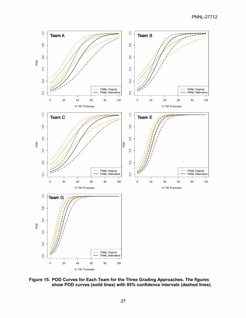
Figure 15 shows the POD curves of each team for the two PNNL grading methods. Compared to Teams A, B, and C, Teams E and G show narrower confidence intervals and steeper slopes, indicating better, more consistent detection performance overall. Also, smaller differences between the POD curves for the different scoring methods suggest that Teams E and G were less affected by the tighter grading units and therefore had overall better axial positioning accuracy.

To further explore how Teams E and G were less affected by the tighter grading units, Figure 16 shows a POD comparison of the two groups of teams (high frequency versus low frequency) for the 36” specimens only (recall that A, B, and C used higher frequency and none of the teams had practice). With the PNNL original grading approach, Figure 16A shows that the 95% confidence intervals of the POD curves for the two groups nearly overlap for most of the flaw size range, although Teams E and G (that used low frequency) consistently outperformed the other teams. However, with the alternative defined grading unit approach, Figure 16B shows that Teams A, B, and C performed significantly worse; i.e., there is little overlap between the confidence bounds of the two groups. This is because the alternative approach, with the grading units that enclosed the true flaws, was much less forgiving than the original approach, where there were no axial limits to grading units. Thus, many reported flaws by the higher-frequency teams that were scored as detections or ignored in the original approach were deemed as false calls in the alternative approach because of poor axial positioning. The performance of the low-frequency teams, on the other hand, was more consistent.

Figure 14. Comparison of POD Curves With and Without FCP. Solid lines are POD and dashed lines show the 95% confidence interval.

PNNL-27712

27

Figure 15. POD Curves for Each Team for the Three Grading Approaches. The figures show POD curves (solid lines) with 95% confidence intervals (dashed lines).

PNNL-27712

28

Figure 16. POD in 36” Specimens for Team Groups. A) PNNL’s original approach. B) PNNL’s alternative approach. The figures show POD curves (solid lines) with 95% confidence intervals (dashed lines).

PNNL-27712

29

8.0 Discussion and Conclusions

The EPRI CASS RRS represents important progress toward understanding current capabilities of flaw detection in CASS piping and the development of Appendix VIII, Supplement 9 performance criteria. The PNNL analyses showed that all teams had FCPs at or below 13%, and teams that used low-frequency probes had FCPs at or below 6%. One team had a detection rate of 90% and a second team above 75%—both of these teams used low-frequency probes. Teams that used higher-frequency probes were less successful overall in identifying flaws and avoiding false calls.

As part of the MOU, PNNL was asked to report on “the conduct of the testing, results of the examinations, and independent data analysis” (see Section 3.0). Results and analysis of the examinations have been detailed above. Below, PNNL has identified several factors in the conducting of the tests that affected the overall outcome of the RRS. These factors should be considered when reviewing any reported results. It is impossible to quantify the significance of each factor, so they are discussed below in no particular order. For many of these factors, the details supporting them cannot be revealed until the mockup information is released. Therefore, they will be discussed in general terms.

• The primary goal of the RRS was to “evaluate the capabilities of currently available NDE techniques” in examining CASS (EPRI 2018). PNNL’s earlier CASS research established that low-frequency (500 kHz) PA is the most effective NDE technique currently available for examining thick-walled CASS (i.e., wall thicknesses greater than about 40.6 mm [1.6 in.]) (Anderson et al. 2007; Anderson et al. 2011; Diaz et al. 2012). In the RRS, the 28” and 36” specimens were 50.8 mm (2.0 in.) and 68.6 mm (2.7 in.) thick, respectively. On these thicker RRS specimens, the two teams (E and G) that used low-frequency probes had higher detection rates and lower FCP than the three teams that used higher-frequency probes. Based on years of NDE CASS research, it is understood that the use of higher frequencies (≥1 MHz) on thick-section CASS materials will lead to increased FCPs and reduced detection rates. To demonstrate the best currently available techniques and to eliminate probe frequency as a variable in future CASS round robins, all participating teams should be required to use low-frequency probes on materials >40.6 mm (1.6 in.) thick.

• PNNL questioned the inclusion of a 12” specimen with the unusual “preexisting ID condition,” as described by EPRI (EPRI 2018). From laser profile imaging, PNNL found that this specimen had up to 37% of the through-wall thickness in the weld region removed from the ID. EPRI stated in their report that “it is unknown whether the weld would have been put in service or if this condition exists in the fleet” but chose to include it in the RRS anyway. Specimens with distinctive and highly unusual ID surface conditions not seen in the field can pose particular challenges to inspectors and may result in a disproportionately high number of false calls. PNNL asserts that this specimen was not representative of field conditions and should not have been included in the RRS.

• The coarse grain structures in CASS can produce high background noise and beam distortion (Crawford et al. 2014), so it is important to understand what fraction of the false calls were due to the material itself versus any added geometries. Thus, PNNL’s grading criteria classified false calls separately from geometry calls. PNNL found that the geometries designed into many of the specimens resulted in a high number of calls (see Figure 3)—far more than were caused by the CASS parent material. ID conditions in two specimens contributed to 57% of EPRI’s false calls and 28% of PNNL’s false calls (in the original analysis). While PNNL supports the inclusion of representative geometries in RRS

PNNL-27712

30

specimens, PNNL believes that several of the added geometries were less representative of typical field ID surface conditions than they were of worst-case scenarios.

• The number of false calls resulting from ID geometrical features was magnified by the manner that EPRI counted false calls. PNNL concluded that the EPRI definition and use of grading units, and subdivision of reported flaws in the presence of added geometries, resulted in a dramatic increase in FCP that did not fairly represent the participants’ performance.

• The inconsistent use of practice appears to have had a significant impact on the overall results. In particular, results from the 12” specimens, where all teams used high-frequency probes, showed that the three teams that did not practice (A, B, and C) had significantly lower detection rates and higher FCPs (see Figures 6 and 7). As EPRI noted, the practice specimens were similar to the RRS specimens except that the true-state of the practice specimens was provided, so practice appeared to have proved helpful to teams in identifying the varied signatures of geometrical features, flaws, and other background signals. The results showed that teams that did not practice indeed appeared to more often report geometrical features as flaws. Furthermore, in PNNL’s experience, practice gives understanding of how limited scan access due to weld crowns affects the ability to detect flaws while giving valuable information about the inspection angles needed. Thus, teams that did not practice may have been affected more by the presence of the weld crowns. Therefore, the issue of inconsistent practice was a confounding variable to the goals of the RRS, namely to the assessment of detection capabilities in CASS. To eliminate practice as a confounding variable in future round robins, all teams should be required to practice on the same specimens over a consistent and specified time period or practice specimens should not be provided to any teams.

• The presence of what EPRI describes as extraneous cracks may have had an effect on the RRS results. These flaws appeared to be a ubiquitous consequence of the induction TF process for growing deep flaws and may have been unavoidable in this application. It was reported by EPRI that these cracks should not interfere with the RRS, because they are much shallower and shorter than the intended flaws; PNNL generally agrees with this assessment. However, EPRI stated that it was possible for “some” (an undetermined number) of these extraneous flaws to be detected. Based on the grading criteria that EPRI used, detection of the extraneous flaws would typically not be a problem unless a team detected and reported an extraneous flaw but, for whatever reason, also failed to report the intended flaw. Because the extraneous flaws are short, any reports of extraneous flaws would not count as detections under EPRI’s minimum length criterion. It is not possible for PNNL to determine how many times extraneous cracks were reported as flaws. Therefore, the overall impact of the extraneous cracks is unclear but should be considered when studying the outcomes of the RRS.

• EPRI provided an RRS protocol to elicit PNNL and other teams’ participation.5 As part of the testing protocol, EPRI required that participating teams submit for review an examination procedure at least 30 days before the scheduled testing period. The EPRI protocol also defined the examination region as extending on both sides of the welds, but the protocol did not state that examinations would be strictly single-sided. PNNL developed a data acquisition and analysis protocol in compliance with the EPRI guidelines that included making detection calls using dual-sided PA-UT examinations (i.e., from both sides of the weld, where possible, as would be applied in the field) and submitting one data sheet for

5 “Cast Austenitic Stainless Steel Non Destructive Evaluation Protocol for Conducting Blind Round-Robin Study.” Doug Kull and Carl Latiolais, March 30, 2015. Non-public document.

PNNL-27712

31

each mockup. Because EPRI accepted the PNNL test protocol as written, PNNL proceeded with, and practiced with, these procedures at PNNL prior to traveling to EPRI. Then, upon initiating the data acquisition protocol at EPRI, the PNNL Team was told that they could not implement the protocol as written. This required immediate changes to the PNNL planned approach, which potentially had a negative impact on performance and reduced the time available for the PNNL Team to obtain all of the PA-UT data originally anticipated. It is unknown if other participating organizations were also affected by unanticipated protocol changes after arriving at EPRI. Nevertheless, prior to hosting an RR, teams should be well informed of whether their protocols comply with the rules and expectations and what changes, if any, will be required for participation in the RRS.

EPRI implemented a length-based detection rule that discarded reported flaws that did not meet a minimum length threshold of at least 50% of the true flaw length, regardless of SNR ratio or the number of teams that made similar calls. Actual flaw profiles, which may have an impact on the detected signals, were unknown (and still are as of this writing). In RRS discussions with PNNL staff, EPRI reported that flaws were “mountain-peak shaped.” Thus, PNNL inferred that the most likely signal response would be near the center of a flaw, at the “peak” of the mountain. With flaws of this shape, the ends of the flaws were assumed to be shallower and were also observed to be more tightly closed (see Section 4.4), both of which can reduce the detectable signal response. The detectable signal is further reduced by signal dropout, attenuation, and inherent noise, which can result in signal loss in CASS. Furthermore, PNNL research has shown that single flaws in CASS are commonly displayed as discontinuous signal responses due to the deleterious sound field issues, such as beam scattering and beam partitioning (Anderson et al. 2007; Anderson et al. 2011; Crawford et al. 2014; Diaz et al. 2017; Diaz et al. 2018; Diaz et al. 2012). The result of the above factors is that detected flaw lengths may be shorter than actual flaw lengths or flaws may appear as multiple flaws instead of one continuous response. Therefore, a minimum flaw length for detection is not appropriate in CASS. In contrast to EPRI, PNNL did not use any length-based detection criteria, since PNNL’s focus was only on detection and not length-sizing accuracy. Furthermore, PNNL felt that if the short detections are de facto filtered out as non-detections, subsequent length root-mean-square error values calculated will be lower than actually supported by the data. The impact of the length-based detection criterion on the results is discussed in Section 5.1.

EPRI’s threshold of success for the RRS was set at ≥80% for the detection rate and ≤20% for FCP. This was based on historical performance demonstration requirements in fine-grained materials, such as carbon steel or wrought stainless steel that have much different sound propagation and attenuation properties than CASS. However, performance demonstration requirements for CASS have not yet been established, and it is well known that the coarse grain structures in CASS pose unique challenges and make this material more difficult to examine. Research into CASS inspections has been ongoing for decades. Although PNNL’s analysis of the RRS shows that the 80/20 POD/FCP performance demonstration threshold in CASS is attainable with current methods and technology (Anderson et al. 2007; Crawford et al. 2015; Diaz et al. 2017; Diaz et al. 2012), the approach ultimately adopted for CASS should differ significantly from those already established for other materials (Chockie and Griesbach 2013). Therefore, PNNL proposes that the POD and FCP thresholds for flaws in CASS, as well as strategies for length and depth sizing, should be evidence-based and evaluated independently of the values (and their bases) that are currently used in Section XI, Appendix VIII Piping Supplements 2, 3, and 10.

PNNL-27712

32

Based on the results of this RR and previous studies in CASS, PNNL concludes that flaw detection in CASS materials is possible with a high degree of confidence and low probability of false calls when the most appropriate, currently available techniques are used (Anderson et al. 2007; Crawford et al. 2015; Diaz et al. 2017; Diaz et al. 2012). In particular, this means using low-frequency, phased-array probes for examining thick-walled (>40.6 mm [1.6 in.]) CASS piping welds. Furthermore, new technologies that are becoming commercially available, such as full matrix capture (FMC) and total focusing method (TFM), may provide additional benefits to flaw detection in CASS. PNNL has not yet evaluated the performance of either FMC or TFM techniques to CASS examinations.

PNNL-27712

33

9.0 References

Anderson MT, SL Crawford, SE Cumblidge, KM Denslow, AA Diaz and SR Doctor. 2007. Assessment of Crack Detection in Heavy-Walled Cast Stainless Steel Piping Welds Using Advanced Low-Frequency Ultrasonic Methods. NUREG/CR-6933, PNNL-16292, U.S. Nuclear Regulatory Commission, Washington, D.C. ADAMS Accession No. ML071020410.

Anderson MT, AA Diaz, AD Cinson, SL Crawford, SE Cumblidge, SR Doctor, KM Denslow and S Ahmed. 2011. An Assessment of Ultrasonic Techniques for Far-Side Examinations of Austenitic Stainless Steel Piping Welds. NUREG/CR-7113, PNNL-19353, U.S. Nuclear Regulatory Commission, Washington, D.C. ADAMS Accession No. ML12011A130.

Bates DJ, SR Doctor, PG Heasler and E Burck. 1987. Stainless Steel Round Robin Test: Centrifugally Cast Stainless Steel Screening Phase. NUREG/CR-4970, PNL-6266, PISC III Report No. 3, U.S. Nuclear Regulatory Commission, Washington, D.C.

Chockie A and TJ Griesbach. 2013. "The Long Journey in the Development of ISI Rules for CASS Piping." In ASME 2013 Pressure Vessels and Piping Conference, p. V01AT01A058. July 14-18, 2013, Paris, France. DOI 10.1115/PVP2013-98112. American Society of Mechanical Engineeers, New York.

Crawford SL, AD Cinson, AA Diaz and MT Anderson. 2015. Phased Array Ultrasonic Examination of Reactor Coolant System (Carbon Steel-to-CASS) Dissimilar Metal Weld Mockup Specimen. PNNL-24920, Pacific Northwest National Laboratory, Richland, Washington. ADAMS Accession No. ML16041A137.

Crawford SL, MS Prowant, AD Cinson, MR Larche, AA Diaz and MT Anderson. 2014. Phased Array Ultrasonic Sound Field Mapping in Cast Austenitic Stainless Steel. PNNL-23393, Pacific Northwest National Laboratory, Richland, Washington. ADAMS Accession No. ML14155A165.

Cumblidge SE, SR Doctor, PG Heasler and TT Taylor. 2010. Results of the Program for the Inspection of Nickel Alloy Components. NUREG/CR-7019; PNNL-18713, Rev. 1, U.S. Nuclear Regulatory Commission, Washington, D.C.

Diaz A, SL Crawford, RE Jacob, MR Larche, M Prowant, MT Anderson and C Nove. 2017. "Status Update of NDE Research at PNNL--CASS/DMW Examination Reliability." In NRC-Industry Technical Exchange Meeting. January 17-19, 2017, Rockville, Maryland. Pacific Northwest National Laboratory. PNNL-SA-123246. ADAMS Accession No. ML17013A628.

Diaz A, RE Jacob, A Holmes, M Prowant and C Nove. 2018. "Update on Progress in CASS Research at PNNL." In Industry-NRC NDE Technical Exchange Meeting. January 16-18, 2018, Rockville, Maryland. Pacific Northwest National Laboratory. PNNL-SA-131575. ADAMS Accession No. ML18012A718.

Diaz AA, AD Cinson, SL Crawford, R Mathews, TL Moran, MS Prowant and MT Anderson. 2012. An Evaluation of Ultrasonic Phased Array Testing for Cast Austenitic Stainless Steel Pressurizer Surge Line Piping Welds. NUREG/CR-7122, PNNL-19497, Pacific Northwest National Laboratory, Richland, Washington. ADAMS Accession No. ML12087A061 and ML12087A063.

PNNL-27712

34

Diaz AA, AD Cinson, SL Crawford, TL Moran and MT Anderson. 2010. "An Ultrasonic Phased Array Evaluation of Intergranular Stress Corrosion Crack (IGSCC) Detection in Austenitic Stainless Steel Piping Welds." In ASME 2010 Pressure Vessels & Piping Division (PVP) Conference, pp. 255-264. July 18-22, 2010, Bellevue, Washington. DOI 10.1115/PVP2010-25799. PNNL-SA-71595.

EPRI. 2018. Nondestructive Evaluation: Cast Austenitic Stainless Steel Round-Robin Study, Summary of Results, Revision 1. 3002010314 Final Report, Electric Power Research Institute (EPRI), Palo Alto, California.

Heasler PG, TT Taylor and SR Doctor. 1993. Statistically Based Reevaluation of PISC-II Round Robin Test Data. NUREG/CR-5410, PNL-8577, U.S. Nuclear Regulatory Commission, Washington, D.C. ADAMS Accession No. OSTI ID: 6503552; Legacy ID: TI93014020.

Heasler PG, TT Taylor, JC Spanner, SR Doctor and JD Deffenbaugh. 1990. Ultrasonic Inspection Reliability for Intergranular Stress Corrosion Cracks: A Round Robin Study of the Effects of Personnel, Procedures, Equipment and Crack Characteristics. NUREG/CR-4908, PNL-6196, U.S. Nuclear Regulatory Commission, Washington, D.C.

Meyer RM and PG Heasler. 2017. Results of Blind Testing for the Program to Assess the Reliability of Emerging Nondestructive Techniques. NUREG/CR-7235, PNNL-24196, U.S. Nuclear Regulatory Commission, Washington, D.C. ADAMS Accession No. ML17159A466.

Ramuhalli P, PG Heasler, TL Moran, A Holmes and MT Anderson. 2017. Reliability Assessment of Remote Visual Examination. NUREG/CR-7246; PNNL-27003, U.S. Nuclear Regulatory Commission, Washington, D.C.

Weber MF and N Wilmshurst. 2017. Addendum to Memorandum of Understanding between U.S. Nuclear Regulatory Commission and Electric Power Research Institute, Inc. on Cooperative Nuclear Safety Research -- Nondestructive Examination (NDE). U.S. Nuclear Regulatory Commission, Washington, D.C. ADAMS Accession No. ML16138A556.