C—1

PLUME: Imaging the Hawaiian Hotspot and SwellRESULTS FROM PRIOR SUPPORT

MELT Experiment (R. S. Detrick, J. A. Orcutt, J. P. Morgan, S. C. Solomon, C. J. Wolfe)Seismological components of the MELT experiment on the southern East Pacific Rise; OCE-94-03697(WHOI); R. S. Detrick; $1,058,637: 5/1/96-4/30/99; OCE-94-06146 (SIO); J. A. Orcutt, J. Phipps Morgan,A. J. Harding; $615,637; 4/1/96-3/31/99; OCE-94-02991 (CIW); S. C. Solomon, C. J. Wolfe, $110,000; 6/1/96-8/31/00. MELT, the largest seafloor geophysical experiment ever undertaken, was aimed atmapping the distribution of melt from its source deep within the mantle to the seafloor beneaththe fast spreading southern East Pacific Rise (EPR) near 17°S. Ocean bottom seismometers (OBSs)from four different groups were deployed along two lines across the rise axis recording over an 8-month period starting in late 1996. The MELT experiment demonstrated for the first time thatgood long-period data could be acquired using OBSs, and it collected the largest teleseismic dataset ever obtained from a seafloor seismic array [MELT Seismic Team, 1998]. The seismic resultsdemonstrated that basaltic melt is present in the mantle beneath the EPR in this area over asurprisingly broad region several hundred kilometers across and extending to depths of greaterthan 100 km [Forsyth et al., 1998; Toomey et al., 1998; Webb and Forsyth, 1998]. This findingcontradicts the predictions of some models that melt would be confined to a narrow region of highconcentration beneath the rise axis. The previously known asymmetry in seafloor depth and off-axis volcanism in this area was shown to be reflected in a strongly asymmetric mantle structure.Mantle densities and seismic velocities are lower [Forsyth et al., 1998; Toomey et al., 1998] andseismic anisotropy is stronger [Wolfe and Solomon, 1998] to the west of the rise axis. However,crustal thickness is essentially the same on the two flanks of the ridge [Canales et al., 1998; Bazin etal., 1998]. The asymmetry in mantle anisotropy was interpreted in terms of spreading-inducedflow above a depth of ~100 km and a deeper return flow from the Pacific Superswell region [Wolfeand Solomon, 1998]. Receiver function analysis using S waves converted from P waves at the 410-and 660-km discontinuities showed a normal transition zone thickness, indicating that upwellingbeneath the southern EPR does not extend into the lower mantle [Shen et al., 1998a].

The Ocean Seismic Network Pilot Experiment (J. A. Collins, J. A. Orcutt)Broadband seismic measurements on the deep sea floor: A pilot experiment; OCE-9522114 (WHOI), OCE-9523541 (SIO); J. A. Collins, J. A. Orcutt, K. R. Peal, F. N. Spiess, R. A. Stephen, F. L. Vernon; Part A:$322,500; Part B: $312,500; 12/5/95-11/30/98. The primary goal of the Ocean Seismic Network (OSN)Pilot Experiment was to learn how to make high-quality broadband (0.003-5 Hz) seismicmeasurements on the seafloor [Collins et al., 1998; Stephen et al., 1998]. The experiment wascarried out at the OSN-1 drill site (ODP Hole 843B) 225 km southwest of Oahu. On the deploymentcruise in January- February 1998, we deployed three broadband seismic instruments: a boreholeseismometer, a sensor buried in the surface sediments, and a sensor resting on the seafloor. Theborehole seismometer was a Teledyne KS54000 similar to the sensors used in the global IRIS/IDAand GSN networks [Stephen et al., 1998]. It was placed in the borehole using the MPL/JOI WirelineReentry System. The seafloor and shallow buried sensors were Guralp CMG-3T seismometers. Inaddition to the broadband seismometers we deployed three conventional OBSs with 1-Hz geophonesensors, differential pressure gauges, a conventional hydrophone, and a current meter. All threeof the broadband instruments recorded data continuously and autonomously on the seafloor fromthe time they were deployed in early February until late May or early June (at least 115 days).Over 50 teleseismic earthquakes were observed on the broadband systems ranging from an mb 4.2event at 90° epicentral distance to the Mw 8.1 Balleny islands earthquake at 91° distance. Signal-to-noise ratios varied depending on frequency band, ambient noise conditions, and sensor design.Preliminary analysis indicates that the borehole system provided comparable quality data to similarcontinental and island stations over the 0.001-5 Hz band. The shallow-buried broadband systemcompared favorably with the borehole system for signals in the frequency band from 0.001 to 0.07Hz [Collins et al., 2000].

SWELL Experiment (J. Phipps Morgan, G. Laske, J. A. Orcutt)A pilot seismic experiment to determine the feasibility of mapping the source of the Hawaiian Swell; OCE95-29707; J. Phipps Morgan, G. Laske, J. A. Orcutt; $222,042; 8/96-12/98. The primary objectives of theSWELL experiment were to demonstrate that inexpensive ocean bottom instruments could bedeployed for long-duration experiments to record Rayleigh waves, and to learn whether records

C—2

PLUME: Imaging the Hawaiian Hotspot and Swellof such surface waves could resolve new information on shallow mantle structure diagnostic ofthe dominant mechanism supporting the swell [Laske et al., 1998,b; Phipps Morgan and Parmentier,1998]. This pilot experiment consisted of two deployments (7.5 and 5 months) of an 8-instrumentarray of SIO L-CHEAPO data loggers with differential pressure gauge (DPG) sensors. Instrumentrecovery was 100%, and all but 3 of the 16 drops resulted in continuous 25-Hz data streams for thefull deployment period. To first order, the data analyzed (in the 17-70 s period range) are broadlyconsistent with predictions for 90-My-old lithosphere. More interestingly, however, there is clearevidence for a strong lateral gradient in structure across the array, with much lower velocitiescloser to the island chain than farther out on the swell [Laske et al., 1999 a,b]. The first deploymentincluded a separate piggy-back MT study by S. Constable at Scripps and G. Heinson and A. Whiteat Flinders University, Australia. Initial inversions indicate a seismicaly slow but electrically highlyresistive swell root [Phipps Morgan et al., 2000].

Hawaiian Scientific Drilling (E. H. Hauri)Scientific drilling in Hawaii: Physics and chemistry of mantle plumes, subcontract “Re-Os isotope analysisof the HSDP Drill Core”; EAR-9528544; E. H. Hauri; $218,075; 7/1/97-6/30/02. This project continuesto support geochemical analyses of Os isotopes in samples from the Hawaiian Scientific DrillingProject on Mauna Kea. Initial results from the 1-km pilot hole [Hauri et al., 1996; Lassiter andHauri, 1998] strongly suggest the presence of a substantial component of recycled oceanic crust inthe Hawaiian plume. This has been confirmed by recent work on oxygen and Hf isotopes [Eiler etal., 1996; Blicher-Toft et al., 1999]. These data, as well as major element data [Hauri, 1996], havebeen used to estimate the location of the Hawaiian plume, with the Loa-trend volcanoes (Loihi,Mauna Loa, Hualalai) predicted to be closer to the plume axis than Kea-trend volcanoes (Kilauea,Mauna Kea, Kohala).

Mantle Plume Lithosphere Interaction (David Bercovici)Mantle plume-lithosphere interaction: An interdisciplinary study of the dynamics of the Hawaiian hotspot;EAR93-03402; D. Bercovici, P. Wessel, J. Mahoney; $220,000; 1/94-12/96. This project involved a grav-ity-current model for sublithospherically spreading plume heads [Bercovici, 1994, Bercovici andLin, 1996]; the cause of double flood basalts [Bercovici and Mahoney, 1994]; the initiation of plumeheads and diapirs at the D” layer [Bercovici and Kelly, 1997]; coalescence and/or clustering ofrising plume heads [Kelly and Bercovici, 1997]; how starting plume heads possibly induce changesin plate motion (Ratcliff et al, 1998); formation of discrete hotspot islands via the interaction be-tween magma percolation and lithospheric flexure [Hieronymus and Bercovici, 1999a,2000a,b,c].

I. Introduction and RationaleHawaii is the archetype hotspot and is presumed to overlie the archetype mantle plume [Mor-

gan, 1971]. Calculated to transport a larger buoyancy flux than any other active plume [Sleep,1990], the Hawaiian hotspot has been the focus of a number of geodynamical and geochemicalmodeling efforts [e.g., Olson, 1990; Ribe and Christensen, 1994; Hawaii Scientific Drilling Project,1996; Hauri et al., 1994; Eiler et al., 1996; Lassiter and Hauri, 1998]. Further, the Hawaiian hotspotand swell offer one of the best-characterized settings to evaluate the interaction of a mantle plumewith oceanic lithosphere well removed from a ridge axis. There are three classes of plume-lithos-phere interactions that have been proposed for such settings, with data from the Hawaiian regionproviding important underpinnings: (1) reheating of the lithosphere [e.g., Detrick and Crough,1978], (2) underplating by a mantle residuum depleted of partial melt [e.g., Jordan, 1979; PhippsMorgan et al., 1995], and (3) horizontal flow of hot asthenosphere sheared by the overlying plate[e.g., Davies, 1988; Olson, 1990; Sleep, 1990]. Defining well the geometry and other physical char-acteristics of the Hawaiian mantle plume, and distinguishing among proposed explanations forthe Hawaiian swell, will require the application of high-resolution seismic imaging techniques,including body wave and surface wave tomography. Motivated by these goals, the Scripps Insti-tution of Oceanography, the Woods Hole Oceanographic Institution, the University of Hawaii,and the Carnegie Institution of Washington propose a joint experiment to image the upper mantleof the Hawaiian hotspot region: the Plume-Lithosphere Undersea Melt Experiment, or PLUME.

C—3

PLUME: Imaging the Hawaiian Hotspot and SwellWhile global mantle tomography has made great strides in the last few years, the resolution of

global and large-scale regional models is still insufficient to discern confidently the details of featuressuch as plumes with dimensions of a few hundred kilometers or less. Several recent studies illustratethe nature of the issues. Global P-wave travel time inversions now show low velocities in theupper mantle of the Hawaiian region [Bijwaard et al., 1998], but horizontal resolution remainslimited to no better than several hundred kilometers in most intraplate oceanic areas and verticalstreaking is considerable. In contrast, Katzman et al. [1998] report high upper mantle velocitiesbeneath the Hawaiian and several other Pacific island chains inferred from an inversion of traveltimes of generalized seismological data functionals and ScS reverberations along the Tonga-Hawaiicorridor. Ji and Nataf [1998] claim to have detected a low velocity anomaly in the lower mantlecentered 200 km northwest of Hawaii by means of scattered P waves, but the robustness of thisresult is uncertain. Ekström and Dziewonski [1998] argue that the central Pacific — including theHawaiian region — is an area of anomalous mantle anisotropy, an effect that complicates inversionsfor isotropic structure.

There are a number of reasons why a high-resolution experiment to image the Hawaiian plumeand its interaction with the lithosphere is particularly timely: (1) an experiment conceptuallysimilar to the one we propose has successfully imaged the plume beneath Iceland, (2) the MELTexperiment has demonstrated the feasibility of imaging the oceanic mantle with teleseismic andregional data using the latest generation of ocean-bottom seismometers, (3) two pilot experimentsin the Hawaiian region — SWELL and PELENET — have verified that there are short-wavelengthvariations in mantle seismic velocity in the area of the Hawaiian hotspot, and (4) with theestablishment of the U.S. National OBS Instrumentation Pool wide-band OBSs are now availablefor the first time in sufficient numbers to make an experiment of this kind feasible at Hawaii.

The ICEMELT experiment in Iceland [Bjarnason et al., 1993] illustrated that teleseismic datafrom a temporary seismic network centered over a hotspot can resolve important details of thestructure of an active mantle plume. In particular, the delay times of teleseismic body waves froma good distribution of back azimuths can recover the three-dimensional P and S wave velocity ofthe upper mantle to a depth comparable to the aperture of the network, or about 400 km for theICEMELT experiment [Wolfe et al., 1997]. The influence of the plume to greater depths can bediscerned by the temperature-induced perturbations to the depths of the 410-km and 660-km mantlediscontinuities as determined from the arrival times of converted phases [Shen et al., 1998b]. Thepattern of mantle anisotropy as revealed by shear-wave splitting measurements further constrainsthe interaction of the asthenospheric flow fields induced by plume divergence and plate motions[Bjarnason et al., 1997]. Data from a larger deployment of broadband seismometers in Icelandsubsequent to ICEMELT, the HOTSPOT experiment, promise to sharpen our view of the Icelandplume [Allen et al., 1999].

That networks of seafloor seismic instruments can conduct mantle imaging experimentscomparable to those now possible with portable broadband land stations was well demonstratedby the MELT experiment [MELT Seismic Team, 1998]. In particular, MELT showed that long-period teleseismic shear waves suitable for imaging [Toomey et el., 1998] and splitting studies[Wolfe and Solomon, 1998] could be recorded by the current fleet of three-component ocean-bottomseismometers. Robust results on lateral variations in structure and anisotropy were best obtainedby a combination of analysis approaches that utilized body and surface waves from both teleseismicand regional phases [Forsyth et al., 1998; Webb and Forsyth, 1998; Toomey et al., 1998; Wolfe andSolomon, 1998; Shen et al., 1998a].

Three small pilot experiments have illustrated the ability of a seismic network in the Hawaiianregion to record data from a good azimuthal distribution of sources and to resolve hints of interestingvariations in mantle structure. The SWELL experiment, two deployments of eight ocean bottomdifferential pressure gauges (DPGs) on the Hawaiian swell, resolved lower Rayleigh-wave phasevelocities near the island chain than farther out on the swell [Laske et al., 1998a,b, 1999a,b]. ThePELENET experiment, a network of seven portable broadband seismic instruments operating onthe Hawaiian Islands, has resolved mantle heterogeneity along the island chain [Wolfe et al., 1998b]and lateral variations in shear wave splitting parameters [Russo et al., 1999]. The Ocean SeismicNetwork Pilot Experiment (OSNPE) provides a baseline for predicting the frequency of detectingteleseismic P and S waves with wide-band ocean bottom seismometers in the Hawaiian region.The products of these pilot experiments, described at length below, provide strong impetus for a

C—4

PLUME: Imaging the Hawaiian Hotspot and Swelllarger experiment to elucidate and understand the mantle velocity structure in three dimensionsand its relation to the Hawaiian plume and its interaction with the Pacific plate.

II. BackgroundDespite the importance of the Hawaiian hotspot to geodynamical and mantle geochemical issues,

seismic constraints from prior global and regional seismic studies of the structure of the lithosphereand asthenosphere in the Hawaiian region are limited and often conflicting. In addition to therecent studies cited above, there have been a number of regional body-wave tomographic andrefraction seismic experiments [e.g., Ellsworth and Koyanagi, 1977; ten Brink and Brocher, 1987;Lindwall, 1988], but these studies have concentrated on the crustal and uppermost mantle structureeither beneath or in the immediate vicinity of the islands. Regional surface-wave studies havebeen carried out with land-based stations [e.g., Woods and Okal, 1996; Priestley and Tilmann,1999]. However, the two-station technique generally used in those studies allows determinationonly of path-averaged structures along relatively long travel paths between the stations. Globalsurface wave studies typically include many crossing paths in this area and are able to resolvelaterally varying structure, but the shortest lateral scale of resolved features in the area currentlyexceeds 500 km. Further, recent global models disagree even for larger-scale features. For example,phase velocity maps for 60-s Rayleigh waves disagree dramatically in a 1500-km wide area aroundHawaii. After long-wavelength trends have been removed from the models, the maps of Laskeand Masters [1996] and Zhang and Lay [1996] show negative velocity anomalies to the southeastof the Hawaiian Island chain, but those of Trampert and Woodhouse [1996] and Ekström et al.

Swell Pilot Experiment (97/98)

existing permanent global st.

planned permanent global st.

land stations

body wave sites

surface wave sites

joint sites

OSN Pilot Experiment (98)

-7.0 -6.5 -6.0 -5.5 -5.0 -4.5 -4.0 -3.5 -3.0 -2.5 -2.0 -1.5 -0.5 0.0 0.2

km

165˚W

165˚W

160˚W

160˚W

155˚W

155˚W

150˚W

150˚W

15˚N 15˚N

20˚N 20˚N

25˚N 25˚N

30˚N 30˚N

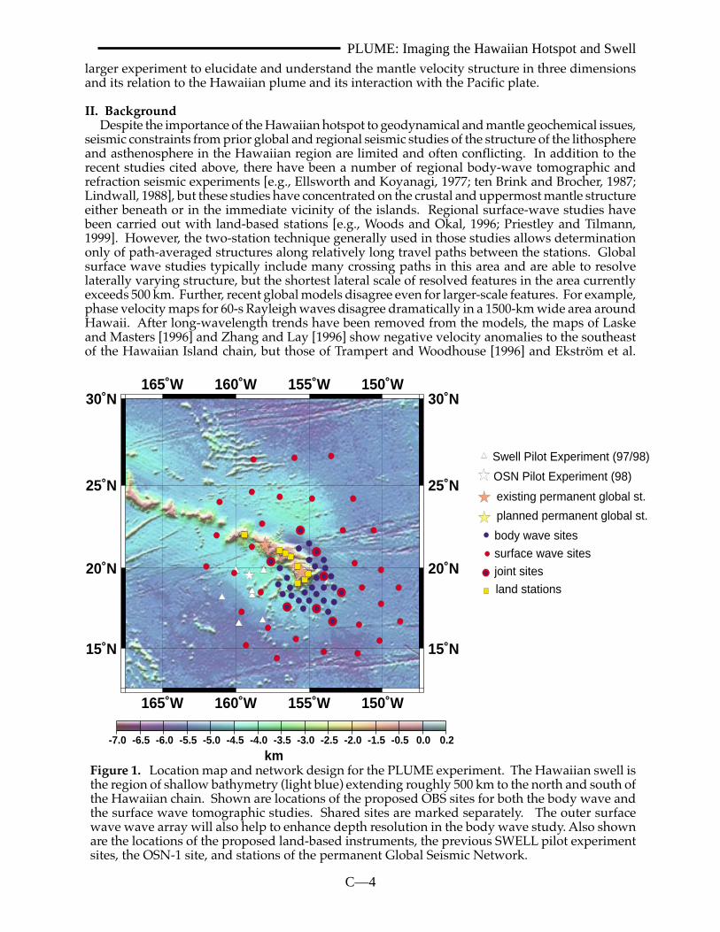
Figure 1. Location map and network design for the PLUME experiment. The Hawaiian swell isthe region of shallow bathymetry (light blue) extending roughly 500 km to the north and south ofthe Hawaiian chain. Shown are locations of the proposed OBS sites for both the body wave andthe surface wave tomographic studies. Shared sites are marked separately. The outer surfacewave wave array will also help to enhance depth resolution in the body wave study. Also shownare the locations of the proposed land-based instruments, the previous SWELL pilot experimentsites, the OSN-1 site, and stations of the permanent Global Seismic Network.

C—5

PLUME: Imaging the Hawaiian Hotspot and Swell[1997] show strong positiveanomalies.

Three recent experiments —SWELL, PELENET, and OSNPE,all involving collaborators onthis proposal — suggest that adense network of seafloor andland seismometers wouldrecover data that can resolve thestructure of the Hawaiianhotspot and swell in sufficientdetail to settle the outstandingquestions on the nature of theplume and its interaction withthe lithosphere.

SWELL. The primaryobjective of the SWELL (SeismicWave Exploration of the LowerLithosphere) experiment was toimage the lithosphere and upperasthenosphere using

intermediate-period (15-80 s) Rayleigh waves. Regional surface wave studies made with temporarybroadband arrays are now in routine use for mapping lithospheric and asthenospheric structureon continents [e.g., Snieder, 1988; Zielhuis and van der Hilst, 1996]. Such studies have beenextremely rare in the oceans, however [e.g., Forsyth et al., 1998]. One reason is that traditionalinstrumentation has not allowed seismologists to record surface waves with high fidelity. The L-CHEAPO instruments recently developed at SIO enable surface waves to be well recorded in thefrequency-band of interest over experiment durations of ~ 1 year.

In 1997-1998 a pilotstudy was carried out ina small region aroundthe OSN boreholeseismometer test site atODP borehole 843Bsouth of Oahu. For theSWELL pilot study,eight L-CHEAPOinstruments usingDPGs were placed in ahexagonal array, at astation spacing of ~220km, to the southwest ofthe Hawaiian Islands(Fig. 1). Six of the eightL-CHEAPOs recordedthe full 7.5 months ofthe first deployment,and seven of eightinstruments recorded the entire 5 months of a second deployment at the same sites. The surfacewave records collected include high-quality waveforms from 82 teleseismic shallow events welldistributed in azimuth (Fig. 2). An example record is shown in Fig. 3. For most of the 82 events,we were able to measure dispersion at periods between 17 and 50 s. The high quality of thewaveforms for some events allowed us to extend the procedure to 70 s, sometimes even beyond.

The average seismic structure beneath the pilot array is similar to that of 90-My-old lithosphere[Nishimura and Forsyth, 1989]. The excellent azimuthal data coverage allowed us to includeazimuthal anisotropy in the modeling process, and we obtained similar results for the isotropiccomponent whether or not we included anisotropy in the model. The amount of anisotropy is

KIP x

x

x

x

x

x

x

x

x

x

x

x

x

x

x

x

x

x

x

x

x

x

x

x

x

x

x

x

x

x

x

x

x x

x

x

x

x x

x

x

Ray Paths to Hawaii (Apr 97 - Dec 97/Dec 97 - May 98)

KIP x

x

x

x

x

x

x

x

x

x

x

x

x

x

x

x

x

x

x

x

x

x

x

x

x

x

x

x

x

x

x

x

x

x

x

Figure 2. Data coverage for the two deployments of theSWELL pilot study. The 48 events of the 7.5-month-long firstdeployment are marked with red dots, while the 34 events ofthe 5-month-long second deployment are marked with or-ange dots (blue dashed ray paths). The azimuthal data cov-erage is good, with gaps only toward the South Pacific Oceanand at azimuths between 0 and 70˚.

Rat Islands Dec17 (351), 97; 04:38:53.0h0=33km; Ms=6.5

bp:0.015-0.05Hz

Epi

cent

ral D

ista

nce

[deg

]

200. 203. 206. 197.

23.

20.

17.

5/6

1 2

3

4

7

8

KIP

aligned on 50s Rayleigh Waves

Figure 3. Example of SWELL data for a Rat Islands event. The bluetrace is the vertical record from GSN station KIP (Kipapa, Oahu).The KIP seismograms are not corrected for instrumental response orconverted to pressure. All records have been bandpass filtered.

C—6

PLUME: Imaging the Hawaiian Hotspot and Swellrather modest (no greater than 2% atperiods of 30- 60 s). The direction offast phase velocity follows the currentplate motion direction for periodslonger than 40 s and the fossilspreading direction for shorter periods,in accordance with a two-layeranisotropic model in which flowinduced by plate shear dominatesanisotropy in the asthenosphere andanisotropy aligned with the fossilspreading direction is ‘frozen’ into thelithosphere.

We were also able to resolve three-dimensional structure by measuringthe dispersion for each two-station legof the pilot array. Maps summarizingthe phase velocities as a function ofperiod suggest only a modest changein phase velocity across the array forshort periods. At periods greater than35 s, however, there is a pronouncedvelocity gradient perpendicular to theisland chain, with anomalously lowvelocities close to the islands.Inversions of the two-stationdispersion curves reveal a moderatelydeep swell root that is restricted to beclose to the island chain (Fig. 4). Theseresults demonstrate clearly that surfacewave tomography carried out with alarger network can resolve the deepstructure of the Hawaiian swell.

PELENET. The CarnegieInstitution has operated a network ofportable broadband, three-componentseismometers — PELENET — in theHawaiian Islands since December

1996. The network initially consisted of four stations on the islands of Hawaii (at South Point),Maui (at Haleakala), Molokai, and Kauai; data from IRIS station KIP (Kipapa) on Oahu have alsobeen available. In August 1998, PELENET was enlarged by Raymond Russo and Emile Okal, ofNorthwestern University, who deployed three additional broadband portable stations on the islandof Hawaii (Hilo, Kohala, and Mauna Loa). Analysis to date has focused on teleseismic body wavearrivals [Russo et al., 1998, 1999; Wolfe et al., 1998a,b], as described below.

Delay Time Tomography. We have analyzed and inverted the relative body wave delays with thesame methods that were applied to the ICEMELT experiment to image the Iceland mantle plume[Bjarnason et al., 1996; Wolfe et al., 1997]. The detectability of teleseismic body waves at Hawaii,however, is lower than in Iceland. The azimuthal distribution of the earthquakes analyzed atPELENET from December 1996 through January 1999 is shown in Fig. 5. We filter the arrivals inthe frequency band 0.05-0.1 Hz for S waves and 0.5-1.0 Hz for P waves. We also incorporatedbroadband OSNPE data into our analysis. We have obtained picks from 57 earthquakes for Swaves and 35 earthquakes for P waves. The azimuthal distribution for events is good between200° and 360° (clockwise from north), but it is poor to the east, where most events are distributedonly between 80° and 110°. In addition to direct P and S waves, we are also able to pick selectedSKS phases. Body wave detectability at PELENET has been limited by the small number of stations;a larger network would substantially increase the percentages of events useful for imaging.

198ß 200ß 202ß 204ß

16ß

18ß

20ß

198ß 200ß 202ß 204ß

16ß

18ß

20ß

100 km 140 km

20 km 60 km V0 = 4.63 km/s V0 = 4.59 km/s

V0 = 4.30 km/s V0 = 4.20 km/s

198ß 200ß 202ß 204ß

16ß

18ß

20ß

198ß 200ß 202ß 204ß

16ß

18ß

20ß

-4.0 -3.0 -2.0 -1.0 0.0 1.0 2.0 3.0 4.0

dV/Vs [%]

Figure 4. Variations of shear velocity across the SWELLpilot array, as a function of depth. This model was ob-tained by inverting the path-averaged two-station ve-locity curves of each leg for shear velocity at depth andthen inverting the path-averaged shear velocity mod-els for true 3D shear velocity. The variations are withrespect to the starting model of Nishimura and Forsyth(1989) for 52-110 Ma lithosphere.

C—7

PLUME: Imaging the Hawaiian Hotspot and SwellP and S wave

tomographic imagesobtained from aninversion of delay timesare shown in Fig. 5.Because of the nearlylinear geometry of thenetwork, three-dimensional anomaliesare not well resolved.The consistent featureresolved independentlyin both P and S waveimages is a low-velocityanomaly in the mantlebeneath Maui andMolokai. Themagnitude of this low-velocity anomaly issmall, about 0.5% for Pwaves and 1% for Swaves, and resolutiontests show that the depthis not well constrained.The amplitude of thisfeature is much smallerthan that of the low-velocity anomalyimaged beneath Iceland,interpreted to be theplume conduit (2% for P

waves and 4% for S waves). The anomaly beneath Maui and Molokai may represent variations inthe temperature of hot, plume-fed asthenosphere flowing parallel to the absolute plate motion.Another obvious feature of Fig. 5 is that we do not resolve a plume-like anomaly near the island ofHawaii with a network consisting only of stations on the islands. Clearly an experiment with abroad and dense network will be required to resolve a plume conduit in the region surroundingHawaii.

Shear-Wave Splitting. Splitting parameters for the core phases SKS and SKKS reflect the path-integrated effects of upper mantle anisotropy beneath the receiver [e.g., Vinnik et al., 1989; Silverand Chan, 1991]. Because olivine is anisotropic and develops lattice-preferred orientation inresponse to finite strain, olivine alignment can reflect anisotropy from plume upwelling andasthenospheric flow, as well as any fossil lithospheric anisotropy, presumably aligned in the fossilspreading direction. Shear-wave splitting results at PELENET stations have been summarized byRusso et al. [1999]; splitting at KIP on Oahu was previously determined by Wolfe and Silver [1998].The splitting parameters at Kauai, Oahu, and Molokai are all similarly oriented along the fossilspreading direction, suggesting that fossil lithospheric anisotropy dominates the splitting signal.A change in anisotropy at Maui and Hawaii may indicate that the contribution to anisotropy ofplume-driven and asthenospheric flow becomes stronger and lithospheric anisotropy becomesweaker toward the present location of the Hawaiian hotspot. These results are broadly consistentwith the observations of anisotropy in the SWELL experiment. A much larger network would testthis suggestion as well as document whether there is a resolvable plume influence on anisotropyin the region.

Receiver Function Analysis. Receiver functions [Langston, 1977] derived from teleseismic bodywaves can be used to detect P-to-S conversions at mantle discontinuities beneath the receivingseismometers. Receiver function analyses have been useful for determining the depths to the 410-and 660-km discontinuities [e.g. Dueker and Sheehan, 1997, Shen et al., 1998a,b], which are expected

station terms (s)

-1-.5.5 1

2221

2019

161 160 159 158 157 156 155 154

depth = 150 km

Longitude West

Latit

ude

-0.5 -0.3 -0.2 0.0 0.2 0.3 0.5

P-wave % slowness anomaly

station terms (s)

-2 -1 1 2

2221

2019

161 160 159 158 157 156 155 154

depth = 150 km

Longitude West

Latit

ude

-2.0 -1.3 -0.7 0.0 0.7 1.3 2.0

S-wave % slowness anomaly

magnitudethreshold

- 0.0- 5.5- 6.0- 6.5

Event locations with respect to Hawaii

P

EAST

NORTH

WES

T

SOUTH

<- az

imuth

->

20

40

60

80

100angular distance

magnitudethreshold

- 0.0- 5.5- 6.0- 6.5

Event locations with respect to Hawaii

S

EAST

NORTH

WES

T

SOUTH

<- az

imuth

->

20

40

60

80

100angular distance

Figure 5. Tomography results from PELENET (top) and azimuthaldistribution of earthquakes used in the delay-time inversions (bot-tom).

C—8

PLUME: Imaging the Hawaiian Hotspot and Swell

to respectively increase and decrease with increasing temperature. In particular, beneath centralIceland Shen et al. [1998b] showed that the mantle transition zone is 20 km thinner than for theaverage Earth, supporting a hot and narrow plume. At this point, only a preliminary stack hasbeen made of receiver functions using one and a half years of data from PELENET [Wolfe et al.,1998a]. A total of 141 receiver functions (about one tenth the number of those used in ICEMELT)has been stacked in seven overlapping stripes along the island chain. We do not observe resolvableP410s or P660s conversions. Our preliminary results differ from other analyses that incorporateddata only from KIP; e.g., Vinnik et al. [1997] observed P410s and P660s phases in stacks of 64 high-quality seismograms at KIP (from 10 years of data). This discrepancy suggests that the data in thepreliminary PELENET analyses are inadequate for discerning the signatures of the 410- and 660-km discontinuities, and that significantly larger data sets will be necessary to resolve these features.

OSNPE. The Ocean Seismic network Pilot Experiment (OSNPE) took place from January toJune 1998. The goal of the OSNPE was to learn how to make high-quality broadband seismicmeasurements in the deep oceans. The experiment site was ODP Hole 843B (site OSN-1) locatedabout 225 km southwest of Oahu, Hawaii (Fig. 1). At site OSN-1, three broadband seismometerswere deployed within 300 m of each other; one was installed in the borehole 242.5 m beneath theseafloor (station OSN1), one was surficially buried in the seabed (station OSN1-B), and one wasdeployed on the seabed (station OSN1-S). Total recording duration varied from instrument toinstrument but ranged from 112 to125 days. Over 150 teleseisms were observed on all three broad-band seismographs, ranging in size from an Ms 4.1 at 53° epicentral distance to the 8.1 Mw BallenyIsland earthquake at 91˚ epicentral distance. The most distant event detected is an Ms 5.8 earth-quake near Prince Edward Island on the Southwest Indian Ridge at 150° epicentral distance.

The results of the OSNPE are relevant to the proposed experiment in that they establish a firmbasis for predicting the number and frequency band of the teleseismic events that might be detect-able with the wide-band ocean-bottom seismographs that we propose to deploy. The most strik-ing result from the OSNPE is the superb quality of the surface-waves and long-period body wavesrecorded by the surficially buried broadband seismometer at station OSN1B [Collins et al., 2000].This station recorded over 200 teleseisms, a large majority in the long-period band. The highsignal-to-noise of the long-period data on all three components – comparable to that of a verygood PASSCAL station - is attributable to the fact that the seismometer was buried in the seabed,and hence was not subjected to tilt accelerations generated by seafloor currents pushing on theseismometer. At long period, the signal-to-noise ratio of station OSN1B is noticeably higher thanthat of the seafloor station OSN1S. This is true for all components but the difference is mostpronounced for the horizontal components. For the seafloor station OSN1S, the lower frequencylimit of useful vertical-component data is ~0.01 Hz. The lower frequency limit of useful horizon-tal-component data is much higher, about 0.1 Hz.

Clearly, any broadband ocean-bottom seismometer should be buried, if possible. Unfortunately,at this time, the technology does not exist to bury all of the 64 seismometers that we propose todeploy on PLUME in a cruise of reasonable length. However, results from OSNPE, and the reso-lution test described later in this proposal, show that a seafloor wide-band instrument can recordan adequate number of measurements of ~1 Hz P-wave travel times and ~0.1 Hz S-wave traveltimes to successfully achieve the goals of this project. This is true even though measurements ofthe ambient noise spectrum at OSN-1 show that noise levels in the short-period band (> 0.1 Hz)are high [Collins et al., 2000]. Indeed, at 1 Hz, vertical-component noise levels for stations OSN1Band OSN1S are ~5 dB greater than those observed at the MELT site [Wilcock et al.,1999]. However,a careful examination of the data from stations OSN1B and OSN1S broadband seismographs shows10 pickable P-wave arrivals and 25 pickable S-wave arrivals during a ~ 4 month deployment inone of the noisier periods of the year (winter/spring). Six of these P arrivals are detectable in theband 0.5-1.5 Hz. The remaining 4 P arrivals are pickable only at slightly higher frequencies of upto 4 Hz. The relatively high detectability at high frequency is presumably a consequence of thefact that the mantle in the vicinity of OSN-1 is relatively non-attenuative and cold. Body-wavemagnitudes for these events ranged from 4.6 to 5.9, epicentral distances from 41°-75°, back azi-

C—9

PLUME: Imaging the Hawaiian Hotspot and Swell

muths from 206° clockwise to286°, and focal depths from 64-652 km. The 25 S arrivals arepickable in the band 0.05-0.1 Hz.As for PELENET, the events thatresult in detectable P-wave arriv-als do not always generate detect-able S-wave arrivals. Body wavemagnitudes for the events thatgenerated detectable S arrivalsranged from 4.6 to 6.1, epicentraldistances from 42° to 107°, back-azimuths from 83° clockwise to350°, and focal depths from 30-652 km. Fig. 6, 7, and 8 show Pand S body wave arrivals re-corded both by the OSNPE andPELENET seismographs fromevents with epicentral distancesranging from 42°-75°. Note thecoherence of the P and S arrivalson all stations.III. ExperimentObjectives

The PLUME experiment hasthree broad objectives: (1) locateand image the plume conduitbeneath the Hawaiian hotspot,(2) image the roots of theHawaiian swell over a sufficientarea and with a sufficientresolution to distinguish amongcompeting hypotheses forplume-lithosphere interaction,and (3) relate the findings from

the seismic imagingexperiments to geodynamicaland geochemical models formantle plumes.

The first major objective ofthe PLUME experiment willbe to image the plumeconduit in the mantle beneathHawaii (Fig. 9). Does theHawaiian plume originate inthe lower mantle or in thetransition zone between theupper and lower mantle?What are the dimensions ofthe plume in theasthenospheric mantle? IsHawaii associated with arelatively broad (>200 km

OSN1-Z

OSN1B-Z

OSN1S-Z

MOLH-Z

MAUH-Z

BIG2-Z

KAUH-Z

2 s

OSN1-R

OSN1B-R

OSN1S-R

MOLH-R

MAUH-R

BIG2-R

KAUH-R

10 s

(a)

(b)

Figure 6. OSNPE and PELENET seismograms of the 29March1998 mb 5.9 (IDC REB) Fiji event. Focal depth is 530km, and the epicentral distance to site OSN-1 is 42°. Theseismometers for the OSNPE stations OSN1, OSN1B, andOSN1S were installed ~240 m below the seafloor, in theuppermost 1.5 m of the seabed, and on the seafloor,respectively. Stations MOLH, MAUH, BIG2, and KAUHare PELENET stations deployed on Molokai, Maui,Hawaii, and Kauai, respectively. (a) P-wave arrivals,filtered 0.5-1.5 Hz. (b) S-wave arrivals, filtered 0.05-0.1 Hz.

OSN1-Z

OSN1B-Z

OSN1S-Z

MOLH-Z

MAUH-Z

BIG2-Z

KAUH-Z

2 s

Figure 7. P-waves from the 23 May1998 mb 5.4 (IDC REB)Mindanao event recorded on the OSNPE and PELENET stations.Focal depth is 652 km, and the epicentral distance to site OSN-1is 75°. Station names are explained in the caption to Fig. 6. Thefrequency passband is 0.5-1.5 Hz.

C—10

PLUME: Imaging the Hawaiian Hotspot and Swellwide), warm (50-100°C) plume or anarrower (<100 km wide), hotter (200-300°C) plume? What are the depth ofmagma generation beneath Hawaiiand the lateral distribution of melt inthe upwelling mantle? What is therelationship between the plumeconduit and the surface expression ofvolcanism? These are first-orderquestions, and they are questions thatcan be readily addressed usingestablished seismic analysistechniques and a seismic networkconsisting of both island and seafloorstations. We will use delay times ofteleseismic P and S body waves toconstruct a three-dimensional imageof upper mantle structure beneathHawaii and determine the location ofthe plume conduit, its width, and the

magnitude of the thermal anomaly and any melt anomaly associated with the plume. Shear-wavesplitting anomalies will be used to constrain flow-induced alignment of olivine grains in the mantlebeneath Hawaii, providing constraints on plume upwelling and asthenospheric flow as well asany fossil lithospheric anisotropy. Finally, receiver function analysis will be used to determine ifthere is a decrease in upper-mantle transition-zone thickness beneath Hawaii, which would beindicative of a lower mantle origin for the Hawaiian plume.

A second major objective of the PLUME experiment is to characterize the interaction betweenthe plume and the lithospheric mantle, in particular to address the origin of hotspot-relatedbathymetric swells (Fig. 1). Is the Hawaiian swell isostatically supported by reheating and thinningof the oceanic lithosphere or by the ponding of low-density mantle residuum at the base of aneffectively normal-thickness lithosphere? Does the horizontal flow of hot asthenospheric materialsheared by the overlying plate play a significant role in forming the swell? What causes the rapiduplift of the swell southeast of Hawaii? The absence of good constraints on upper mantle velocitystructure over the broad area of a swell (>1000 km across) has made it impossible to answer theselong-standing questions. However, with the development of ocean bottom seismic instrumentsthat can record intermediate-period (15-80 s) Rayleigh waves it is now possible to distinguishamong these competing models by conducting the same kind of regional surface-wave studyroutinely used for mapping upper mantle structure on the continents. We will determine thethree-dimensional upper mantle velocitystructure across the entire width of theHawaiian swell and determine if thedensity anomaly supporting the swell isconfined to lithospheric depths (<100km) or located within the underlyingasthenosphere. Depth-dependentanisotropy will be used to map the flowof plume and asthenospheric material asit spreads out at the base the lithosphere.

The third major goal of the PLUMEexperiment will be to integrate the newseismic constraints we obtain on plumegeometry and plume-lithosphereinteraction with geochemical andgeodynamical constraints on uppermantle dynamics. For example, temporalvariations in eruption rates, major andtrace elements, and isotope studies have

OSN1-Z

OSN1B-Z

OSN1S-Z

MOLH-Z

MAUH-Z

BIG2-Z

KAUH-Z

2 s

Figure 8. S-waves from the 5 May1998 mb 5.3 (IDCREB) Mariana Islands event recorded on the OSNPEand PELENET stations. Focal depth is 164 km, and theepicentral distance to site OSN-1 is 53°. Station namesare explained in the caption to Fig. 6. The frequencypassband is 0.05-0.1 Hz.

?

?

?Teleseismic Body Waves

Surface Waves

?

? ? Asthenosphere

Lithosphere

?

Plume Conduit

?

?

? mantle residue fromhotspot melting?

initiation ofhotspot melting?

dragging/pondingof hot plume

material?

? ?Plume Head

Figure 9. Schematic representation of possible aspectsof a plume beneath the Hawaiian hotspot and its inter-action with the lithosphere beneath the Hawaiian swell.

C—11

PLUME: Imaging the Hawaiian Hotspot and Swellbeen used to estimate the location, size, and temperature of the Hawaiian plume [Hauri, 1996;DePaolo and Stolper, 1996; Hauri et al., 1996]. However, these estimates are highly uncertain andmodel-dependent. A direct determination of the lateral extent of the Hawaiian plume at depth inthe mantle will provide critical ground truth for these models. By determining whether theHawaiian plume originates in, or penetrates through, the 660-km discontinuity, we will providefundamental new information on the layering of convection in the Earth’s mantle. To address thebroader implications of our investigation of upper mantle seismic structure beneath Hawaii wehave included three individuals in our research team who have extensive experience in plumegeochemistry (Erik Hauri) and geodynamical modeling of plumes and plume-lithosphereinteractions (David Bercovici and Jason Phipps Morgan).

IV. Experiment PlanOur experiment involves the deployment of 64 wide-band ocean-bottom seismic instruments

and 10 portable broadband seismic instruments on land (Fig. 1) for a total network operationduration of 15 months. To take advantage of the period of low wind speeds, the proposed OBSdeployment will extend over two fall seasons. The portable land stations, to be provided by CIW,will all consist of Streckeisen STS-2 three-component seismometers and Reftek 24-bit dataloggers.An inner subnetwork of 33 four-component, wide-band OBSs plus the broadband land stations isdesigned primarily to image the Hawaiian plume conduit by means of body wave tomography.Inter-station spacing within this subnetwork is approximately 75 km. An outer subnetwork of 39wide-band OBSs, all equipped with DPGs, is designed for surface wave tomographic imaging ofthe lithosphere and asthenosphere beneath and outward of the Hawaiian swell, as well ascomplementary body wave observations. Eight of the 64 OBSs are joint sites for both the body-wave and surface-wave tomography portions of the PLUME experiment.

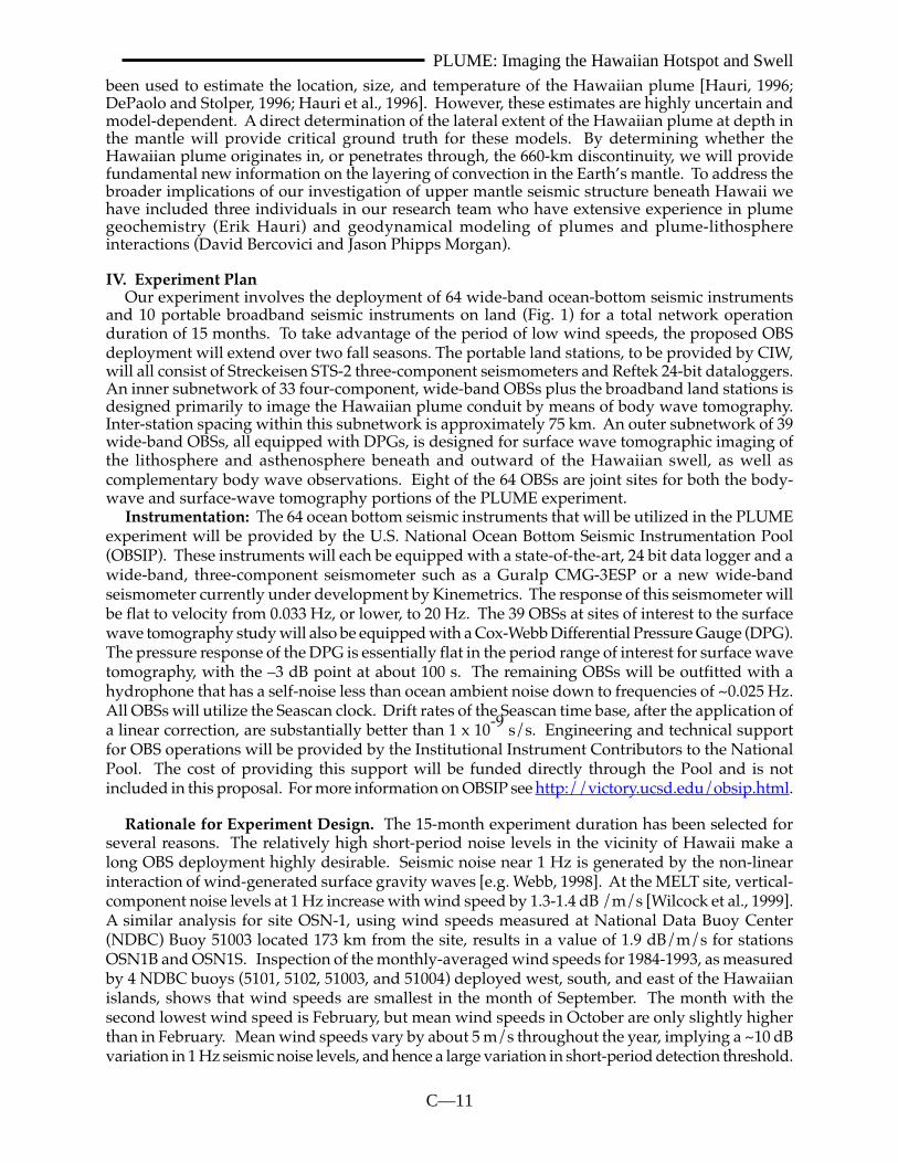
Instrumentation: The 64 ocean bottom seismic instruments that will be utilized in the PLUMEexperiment will be provided by the U.S. National Ocean Bottom Seismic Instrumentation Pool(OBSIP). These instruments will each be equipped with a state-of-the-art, 24 bit data logger and awide-band, three-component seismometer such as a Guralp CMG-3ESP or a new wide-bandseismometer currently under development by Kinemetrics. The response of this seismometer willbe flat to velocity from 0.033 Hz, or lower, to 20 Hz. The 39 OBSs at sites of interest to the surfacewave tomography study will also be equipped with a Cox-Webb Differential Pressure Gauge (DPG).The pressure response of the DPG is essentially flat in the period range of interest for surface wavetomography, with the –3 dB point at about 100 s. The remaining OBSs will be outfitted with ahydrophone that has a self-noise less than ocean ambient noise down to frequencies of ~0.025 Hz.All OBSs will utilize the Seascan clock. Drift rates of the Seascan time base, after the application ofa linear correction, are substantially better than 1 x 10-9 s/s. Engineering and technical supportfor OBS operations will be provided by the Institutional Instrument Contributors to the NationalPool. The cost of providing this support will be funded directly through the Pool and is notincluded in this proposal. For more information on OBSIP see http://victory.ucsd.edu/obsip.html.

Rationale for Experiment Design. The 15-month experiment duration has been selected forseveral reasons. The relatively high short-period noise levels in the vicinity of Hawaii make along OBS deployment highly desirable. Seismic noise near 1 Hz is generated by the non-linearinteraction of wind-generated surface gravity waves [e.g. Webb, 1998]. At the MELT site, vertical-component noise levels at 1 Hz increase with wind speed by 1.3-1.4 dB /m/s [Wilcock et al., 1999].A similar analysis for site OSN-1, using wind speeds measured at National Data Buoy Center(NDBC) Buoy 51003 located 173 km from the site, results in a value of 1.9 dB/m/s for stationsOSN1B and OSN1S. Inspection of the monthly-averaged wind speeds for 1984-1993, as measuredby 4 NDBC buoys (5101, 5102, 51003, and 51004) deployed west, south, and east of the Hawaiianislands, shows that wind speeds are smallest in the month of September. The month with thesecond lowest wind speed is February, but mean wind speeds in October are only slightly higherthan in February. Mean wind speeds vary by about 5 m/s throughout the year, implying a ~10 dBvariation in 1 Hz seismic noise levels, and hence a large variation in short-period detection threshold.

C—12

PLUME: Imaging the Hawaiian Hotspot and Swell

To take advantage of the period of low wind speeds, a 15-month experiment extending over twofall seasons would be highly desirable. Fifteen months is also currently the maximum time theOBSs can operate without a pick-up/redeployment visit.

The two SWELL deployments have shown that a 12-month recording period would probablybe sufficient for the surface wave study alone, but only if Pacific seismicity is as high as in the first7.5 months of that experiment, an unusually active period for large-magnitude events. The OSNPEand PELENET experiments also support a 12-month duration as an absolute minimum for collectinga sufficient set of teleseismic body wave arrivals for tomographic inversion and favor a longerdeployment if possible. The results from the OSNPE provide a firm basis for predicting the numberand frequency band of the teleseisms that might be detectable with wide-band ocean-bottomseismographs during a 15-month deployment. During the 4-month OSPNE (conducted duringthe winter months) 10 pickable teleseismic P-wave arrivals and 25 S-wave arrivals were recordedat this site (cf. Fig. 6). Extrapolating this for a 15-month deployment we can reasonably expect torecord close to 40 pickable P-waves and > 90 pickable S-waves from teleseismic events. Asdocumented by the resolution tests described below, these figures yield more than enoughobservations for the proposed work. This estimate is conservative given that the OSNPE wasconducted in a particularly noisy time of year. This number of events will also help maximize theazimuthal coverage in order to provide as many crossing wave paths as possible for the tomographicimaging.

The SWELL experiment has shown that the bandwidth of the data from the DPG sensors wasessential to retrieve the three-dimensional seismic structure beneath the pilot array. While data atperiods less than 50 s are usually recorded with high fidelity by current ocean bottom instruments,data at longer periods are much more difficult to record but are indispensable to constrain structuresignificantly below 80 km depth using surface wave techniques. It is for this reason that all of thewide-band OBSs in the outer subnetwork will also be equipped with a DPG. Thirteen of theinstruments in the inner subnetwork will also carry DPGs and can therefore provide additionaldata for the surface wave work. The OBSs will all record Love waves, which will provide importantcomplementary data to the primary Rayleigh wave data set.

Resolution Tests. To demonstrate that the inner instrument subnetwork shown in Fig. 1 canimage the plume conduit beneath the hotspot with body wave tomography, we carried out aseries of synthetic experiments, or resolution tests, for P and S wave velocity by means of thefollowing procedure. We first selected a subset of earthquakes spanning a one-year period thatprovided data for the PELENET P- and S-wave tomography. For direct P phases, this set consistedof 17 earthquakes; for direct S waves, this set consisted of 23 earthquakes; one earthquake yieldedSKS arrivals. The azimuthal distributions are similar to those in Fig. 5. These earthquake locationswere then used to create synthetic arrival time data at the PLUME stations for possible plumemodels. In practice, we expect that not all seismometers will necessarily provide phase picks forevery earthquake, but we also expect that the larger network, and the 15-month deployment, willincrease the numbers of useful earthquakes picked. Note for comparison that MELT recorded 20useful earthquakes over a 6-month deployment, although the number of arrivals picked was only175 for P, 154 for Sslow, and 171 for Sfast for about 20-25 working seismometers. Given this lesserreturn rate, we conducted tests with both a 100% and a 50% return rate. For the 100% return rate,all 43 stations provide coverage, whereas for the 50% return rate, we employed a random numbergenerator to give each arrival about a 50% probability of being selected for inclusion in the inversion.The input for the 50% return rate was 512 rays for S waves and 354 rays for P waves, whereas itwould be about twice these amounts in the case of a 100% return rate. We added random (Gaussian)noise with standard deviations of 50 ms for P waves and 300 ms for S waves and inverted the datafollowing Wolfe et al. [1997].

An example of a synthetic input model and the resulting output model for an S-wave inversionis shown in Fig. 10 for a plume conduit located southeast of the 1543-1557 island of Hawaii, adoptingthe more conservative 50% return rate. We assumed a Gaussian plume anomaly with 2% peakamplitude for P waves and 4% amplitude for S waves, similar to the amplitude of the low-velocityanomalies imaged by ICEMELT [Wolfe et al., 1997]. The radius of the plume is 75 km. We alsoinclude a shallow low-velocity anomaly approximately parallel to the Hawaiian Islands to simulatethe effects of hot asthenosphere dragged northwestward by the motion of the Pacific plate [Davies,1988; Olson, 1990; Ribe and Christensen, 1994]. The resulting inversion recovers the general

C—13

PLUME: Imaging the Hawaiian Hotspot and Swell

characteristics of the input anomalies, although the width of the plume is somewhat broadenedand the amplitude is significantly decreased. We obtain a similar-resolution image for the P waveinversion (not shown) with 50% return rate. For comparison, inversions using a 100% return rateincrease the amplitude of the low-velocity anomaly and decrease the amount of broadening of therecovered plume. We expect that the numbers of arrival times in the actual data set will likely besomewhere in between these most optimistic and most conservative extremes and that the PLUMEexperiment will thus be capable of producing a high-quality image of the Hawaiian plume conduit.

Of course, we do not know the location of the Hawaiian plume on the basis of PELENET orSWELL results. For that reason, the stations in the exterior subnetwork (those to be used primarilyin the surface wave inversions) closest to the interior subnetwork will provide extra body wavecoverage in case the center of the plume conduit lies near the edge of the interior network or incase the plume is significantly wider than expected. These stations have not been included in theresolution tests described above, but data from all sites in the exterior subnetwork will both broadenthe lateral coverage and extend the resolution of the body wave imaging to greater depths than inthe synthetic experiments.

Logistics. PLUME will require two 6-week legs, separated by 15 months, for instrumentdeployments and recoveries. Because of the large number of instruments involved we will requirea Melville or Revelle class vessel for both legs. The deployment cruise will need to be scheduledfor late July-August 2001 in order to record during two low-noise autumn seasons. The recoveryleg will take place in November-December 2002. We will require a multibeam profiling capabilityon the deployment ship to aid in site selection. During OBS deployment and recovery operations(perhaps every 2nd or 3rd day), we will take the opportunity to dredge a limited number of seafloortargets on the flexural arch of the Hawaiian swell that have been undersampled. These “archvolcanic fields” have so far yielded young alkalic lavas with geochemical similarities to Hawaiianlavas [e.g., Clague et al., 1990] and are likely to be the products of magmatism at the extreme edgesof the Hawaiian plume. Preliminary geochemical analyses on these samples will be conducted at

2221

2019

1817

161 160 159 158 157 156 155 154 153 152

depth = 250 km

Longitude West

Latit

ude

-4.0 -2.7 -1.3 0.0 1.3 2.7 4.0

S-wave % slowness anomaly

400

300

200

100

0

Dep

th (

km)

2221

2019

1817

161 160 159 158 157 156 155 154 153 152

depth = 250 km

Longitude West

Latit

ude

-2.5 -1.7 -0.8 0.0 0.8 1.7 2.5

S-wave % slowness anomaly

400

300

200

100

0

Dep

th (

km)

Figure 10. Resolution test for PLUME body wave tomography. Left images show the inputmodel, while right images show the inversion solution. See text for further details.

C—14

PLUME: Imaging the Hawaiian Hotspot and Swellno cost to this project.

The installation of the 10 PLUME land stations will follow the methods successfully employedfor PELENET and other CIW broadband seismometer deployments. There will be two types ofsites. Outdoor sites are constructed by digging a hole down to bedrock, burying vertically a portionof a 55-gal steel drum, constructing a cement base, and placing the seismometer on the base withinthe drum. These sites operate on solar panels, with batteries for backup power. Indoor sites willbe on the ground floors of existing buildings and will run off local power with batteries for backup.Both types of sites will include GPS receivers to maintain accurate time. We have already identifiedseven good sites from the PELENET deployment, which we will reoccupy. Our contacts on theHawaiian Islands will help us to identify three additional sites for PLUME. The land stations willbe serviced every 3 months to download data and to ensure that the seismometers are operating.Stations will be installed approximately 3 months prior to the OBS deployments, to ensure thatnoise levels are acceptable at the selected sites. Network operation will continue until all OBSinstruments have been recovered, to ensure maximum overlap with the seafloor records. A totalof eight trips of CIW personnel to Hawaii will be required: one to install the stations, six forservicing, and one to retrieve the instruments.

V. Science Analysis PlanThe analysis tasks that will be carried out with PLUME data, and the individuals who will lead

each task, are as follows:Body Wave Analysis. Teleseismic body waves will be analyzed for three-dimensional mantle

structure, anisotropy, and mantle transition zone structure using established methods previouslyemployed for such other data sets as those from as ICEMELT, MELT, and PELENET. All 64 siteswill be equipped with 3-component, wide-band seismometers that will be useful for each of thebody wave analyses described below. We merely outline the expected analyses here, and we referthe reader to the cited references for additional details.

Body-wave Imaging (led by Wolfe and Solomon). Following the methods applied to ICEMELTand PELENET data (Fig. 5) [Wolfe et al., 1997, 1998a,b], delay times will be determined using themulti-channel cross correlation technique of VanDecar and Crosson [1990]. The delay times willthen be inverted following the methodology of VanDecar et al. [1995]. On the basis of the exten-sive resolution tests described above, we expect that a plume conduit broadly similar to that be-neath Iceland will be well resolved by this experiment.

Shear-wave Splitting (led by Collins, Detrick, Solomon, and Wolfe). Shear-wave splitting at allinstruments will be analyzed to provide information on the flow-induced ordering of olivine grains,which can be used to test models of lithospheric reheating and asthenospheric flow as well as toevaluate the influence of anisotropy on surface and body waves. We will utilize the stackingmethod of Wolfe and Silver [1998], which was applied to the MELT data set [Wolfe and Solomon,1998] to resolve splitting parameters at 18 OBSs from 6 months of data. The method has also beensuccessful in constraining splitting at PELENET [Russo et al., 1999]. We expect that 15 months ofPLUME data will be sufficient for resolving splitting parameters well in the Hawaiian region.

Receiver Functions (led by Collins and Detrick). Receiver function analyses [Langston,1977] willbe undertaken to provide information on the possible influence of plume upwelling on the depthsof upper mantle discontinuities. Since phases generated by conversions at mantle discontinuitiesare often poorly resolved on individual seismograms [van der Lee et al., 1994], we expect thatstacking methods [e.g., Dueker and Sheehan, 1997; Shen et al., 1998a,b] will be necessary to imagethe mantle discontinuity structure beneath the array. Analyses of receiver functions will followthe methods applied to data from MELT [Shen et al., 1998a], ICEMELT [Shen et al., 1998b], andPELENET [Wolfe et al., 1998]. These studies demonstrate that receiver functions can be used toobtain information on mantle transition zone thickness in oceanic settings sufficient to distinguishamong hypotheses for mantle flow patterns.

Surface Wave Analysis (led by Laske and Orcutt). In the SWELL pilot study, the frequency-dependent phase at one station was measured with respect to that of all the others, using a methodsimilar to the multi-taper transfer function technique of Laske and Masters [1996]. The phasemeasured for one station, for each event, is then the statistical average of all individualmeasurements. We will use a similar technique for the PLUME experiment by choosing subsets ofstations to measure the differential phase with high accuracy. Our measurement technique currentlyallows us to obtain stable measurements for earthquakes with magnitudes down to MS=5.5. Smaller

C—15

PLUME: Imaging the Hawaiian Hotspot and Swellevents can be included if attention is restricted to periods less than 40 s.

Phase Velocity Maps. We plan to perform a two-step direct matrix inversion for the three-dimensional (3-D) velocity structure of the lithosphere and asthenosphere beneath the PLUMEnetwork. The first step involves the conversion of the phase measurements to maps of local Rayleighwave phase velocity within the array, as a function of frequency. The second step is a smoothedinversion of these maps into 3-D structure [Masters et al., 1996; Laske et al., 1999b].

Three strategies are available for the first step in the two-step process: (1) invert all phase datadirectly [e.g., Forsyth et al., 1998], (2) invert only phase data that meet the geometrical criteria of atwo-station technique, and (3) build sub-arrays of 3-4 adjacent stations and determine the averagedispersion within each sub-array. Utilizing the first strategy requires correcting the phase data forany contributions due to propagation between the seismic source and the study area. Numericaltests show that differences in phase accumulated along the travel path from the source to theboundary of the study area, using different phase velocity maps, can be similar to the phasedifference accumulated between two adjacent stations. Hence, we plan to start with approaches 2and 3, even though approach 2 implies a reduction in data and approach 3 implies a ‘loss’ oflateral resolution.

In approach three, we determine average phase velocities in each subarray. In a multi-parameterleast-squares procedure similar to that of Stange and Friederich [1993], we fit spherical incomingwavefronts to all phase measurements simultaneously at each frequency. We also solve for afrequency-dependent arrival angle, which accounts for the diversion of the wave packets from agreat circle by lateral heterogeneity. Our experience with the SWELL pilot array is that a sphericalwave is the only perturbation from a plane wave necessary to fit the data. The spherical wavefrontfitting process will be applied to the data of all events simultaneously to determine a ‘referencephase velocity curve’ that describes the average dispersion across each subarray. We anticipatethat lateral structural variations within each array are sufficiently small that the curves obtainedrepresent good estimates of the true dispersion in that area. The curves can then be combined toobtain relatively ‘low-resolution’ but unbiased frequency-dependent phase velocity maps for theentire PLUME study area.

Azimuthal Anisotropy. The spherical-wave fitting process will also be applied for each eventseparately. For each three-station array, phase velocity curves will be available as a function ofazimuth. Any variation with azimuth is most likely attributable to anisotropy within the array,since effects due to propagation outside of each array are eliminated. Azimuthal anisotropy ofphase velocity is typically parameterized as a truncated trigonometric power series [Smith andDahlen, 1973]. In the SWELL pilot study, this approach has worked extremely well [Laske et al.,1999a,b]. In order to interpret azimuthal anisotropy in terms of depth-dependent anisotropicstructure, we will use the formalism of ‘vectorial tomography’ of Montagner and Nataf [1988].This technique has been used successfully in global and regional inversion for anisotropic uppermantle structure [Montagner and Jobert, 1988; Montagner and Tanimoto, 1991]. The method yieldsthe five depth-dependent elastic parameters necessary to describe an anisotropic medium withhexagonal symmetry plus two angles to describe the orientation of the fast direction.

Other Surface Wave Observations. All OBSs will also record Love waves, though low-noise Lovewave recordings are difficult to obtain with the required quality (D.W. Forsyth, personalcommunication). The three components of the seismometer also permit the determination ofparticle motion and thus the direction of approach of the surface wave packets. In global studies,such data are extremely useful for constraining shorter-wavelength structure (Laske, 1995). In thePLUME study, a comparison of these particle motion observations with arrival angles obtainedfrom the sub-array analysis will help in constraining local anisotropy.

Integration with Geochemistry and Geodynamics (led by Hauri, Bercovici, and Phipps Morgan).A tomographic image of the Hawaiian plume, more so than for any other hotspot, would havegreat importance for volcanological, geochemical, and dynamical models of mantle convectionand hotspot magmatism. Direct observations of the location and geometry of the plume wouldprovide vital ground truth to volcano growth models that define the classical framework fordescribing the evolution of oceanic volcanoes [e.g., Clague and Dalrymple, 1987; Lipman, 1995;Hieronymus and Bercovici, 1999].

Location of the Plume. Petrological and geochemical predictions of plume location suggest thatthe plume is centered between the summits of Loihi and Mauna Loa volcanoes [DePaolo andStolper, 1996; Hauri et al., 1996], with the implication that the Loa-trend volcanoes (Loihi, Mauna

C—16

PLUME: Imaging the Hawaiian Hotspot and SwellLoa, Hualalai) are predicted to be closer to the plume axis than Kea-trend volcanoes (Kilauea,Mauna Kea, Kohala). However, these predictions are highly uncertain and model-dependent andwould benefit greatly from a direct seismic image of the sub-Hawaiian mantle. The trajectory ofthe plume stem with depth from this sublithospheric point is, of course, even more uncertain.However, in the proposed study the aperture of the array is large enough to resolve the influenceof the plume (through direct imaging and receiver function analysis of transition zone structure)down to approximately 670 km depth and should thus see both a plume stem (if it is present) aswell as its “pinching” of the transition zone between the 410- and 660-km phase changes. Theresolution of plume stem trajectory with depth would not only give the all-important evidence fora plume but could also be used to infer important properties such as plume velocity. For example,both stem trajectory and the location of the plume stem relative to the swell are primarily func-tions of over-riding plate velocity and average plume ascent velocity. The trajectory of the plumestem is largely governed by the bending of the plume in plate-induced mantle shear [Richardsand Griffiths, 1988]; e.g., little bending occurs when plume material moves much faster than aplate. Second, where the plume stem effectively intersects the sublithospherically-flowing plume-top is determined by how far upstream the plume material can flow before being swept down-stream in the plate direction [Sleep, 1990]. Thus, at the simplest level, the seismically resolvedplume structure and trajectory could be combined with plate velocity data to infer plume veloci-ties and flux. These quantities could be used to greatly refine estimates of plume flux based pri-marily on swell topography [Davies, 1988; Sleep, 1990] and would thus have significant implica-tions about the mode of heat and mass transfer within the Earth. These estimates can be madewith both simple plume stem and plume top models [Richards and Griffiths, 1988; Sleep, 1990;Bercovici and Lin, 1996] or more sophisticated models [Ribe and Christensen, 1994, 1999] to takeinto account additional complexities such as viscous stratification, dependence of plume viscosityon cooling and melting, and chemical buoyancy.

Temperature and Depth of Melting. Geochemical studies of Hawaiian lavas and melt inclusionshave provided consistent estimates of the temperature of the sub-Hawaiian mantle [e.g., Sobolevand Nikogosian, 1994] but place few quantitative constraints on the depth of magma generation.The magnitude of P and S velocity anomalies beneath Hawaii will permit a direct estimate of thesub-Hawaiian temperature distribution. With independent temperature estimates from petrol-ogy, the seismic data will permit tests for the presence of melt beneath Hawaii and perhaps evenits lateral distribution. Several studies of H2O and other volatiles in Hawaiian glasses have led tothe conclusion that the Hawaiian mantle has similar abundances of volatiles to the upper mantlesource of MORB [e.g., Hauri, 1999; Dixon and Clague, 1999]. This observation may simplify theinterpretation of observed velocity anomalies beneath Hawaii.

Plume-Lithosphere Interaction. We will also compare the observed seismic velocity structure be-neath Hawaii with predictions of recent three-dimensional plume-lithosphere interaction models.The model of Phipps Morgan and Parmentier [1998], for example, predicts that melting begins atdepths of 150-200 km beneath Hawaii and persists continuously beneath the swell for more than 5My after passage over the plume. In contrast, the model of Ribe and Christensen [1999] predictsthat melting essentially ceases between Hawaii and Maui after 1 My, with only a minor secondarymelting pulse 3-4 My later. These two models also make quite different predictions for the distri-bution of the thermal anomaly due to motion of the Pacific plate. The wide spatial coverage of theproposed experiment will allow us to test these model predictions, and in particular to determinethe mantle flow conditions necessary to explain simultaneously the seismic structure of the plumeconduit, the swell root, and the region of melting.

Layering of Mantle Convection. Elevated 3He/4He isotope ratios have often been used to infer alower-mantle origin for the Hawaiian plume [e.g., Craig and Lupton, 1976; Kurz et al., 1983], butthis inference has always depended critically on the assumption that mantle convection is suffi-ciently layered that slabs and plumes do not penetrate the 660-km discontinuity. Both of thesepersistently controversial issues can be addressed by measuring the thickness of the transitionzone beneath Hawaii. In view of the increasing evidence for slab penetration into the lower mantle[e.g., van der Hilst et al., 1997], the geochemical arguments for layered convection are becomingever more equivocal. The PLUME experiment provides the opportunity to help resolve this cross-disciplinary paradox by determining whether active upwellings originate in or (as bebeath Ice-land) penetrate through the 660-km discontinuity. The implications of the results of the PLUMEexperiment for the age-old argument of layered versus whole-mantle convection are obvious.

C—17

PLUME: Imaging the Hawaiian Hotspot and SwellVolcano Evolution. Finally, the PLUME experiment comes at a particularly active stage of

geochemical research in Hawaii. Detailed stratigraphic sampling of Mauna Kea volcano contin-ues with the ongoing Hawaii Scientific Drilling Project (HSDP), which has as its goal the recoveryand geochemical study of a continuous drill core through most of the history of this volcano (tar-get depth 14,000 ft; current depth ~8,000 ft with ~90% recovery). A similarly detailed geochemicalhistory of Mauna Loa volcano will soon be augmented by deep submersible sampling of a largefault scarp off the southwest rift zone [Rhodes et al., 1997]. Together, these geochemical data setswill comprise the most complete examination of volcano evolution to date, and their integrationwith high-resolution seismic images of the sub-Hawaiian mantle will provide an unprecedentedopportunity to reveal in detail how intraplate volcanism and swell formation are related to theseismic velocity structure of the underlying mantle.VI. Data Archiving Plan

The PLUME data set will be unique and is likely to be of interest to investigators for many yearsto come in studies that may go far beyond those described in this proposal. To facilitate theutilization of this data set we will permanently archive the PLUME data at the Incorporated ResearchInstitutions for Seismology (IRIS) Data Management Center (DMC) in Seattle. All data will bearchived in the Scientific Exchange of Earthquake Data (SEED) format. The OBS operating groupswill be responsible for providing information on instrument response and transcribing the datafrom PASSCAL SEGY-format into the SEED format before they are transmitted to the IRIS DMC(as was done for the OSNPE). CIW will be responsible for converting data from the portable landstations to miniSEED files and will send data and ancillary information to the IRIS DMC on DLTtapes. The entire data set will also be stored and archived on the on-line AMASS DLT mass storagelibraries at both Scripps/IGPP and WHOI to facilitate data access by all of the investigators involvedin this project. This approach reflects the data management goals in both the funded WHOI andSIO OBS pool proposals. As noted earlier, the pools will be fully operational by the time thisexperiment is conducted. We plan initially to limit data access to investigators associated withthis proposal for a 24-month period after the recovery of the instruments in Year 2 of this project.After this 24-month period the data will available to any interested investigator through the IRIS/DMC.