planning tool of point to point optical communication … · planning tool of point to point...
TRANSCRIPT
Planning Tool of Point to Point Optical Communication
Links
João Neto Cordeiro
Thesis to obtain the Master of Science Degree in
Electrical and Computer Engineering
Supervisor(s): Prof. Paulo Sérgio de Brito André
Prof. Pedro Renato Tavares de Pinho
Examination Committee
Chairperson: Prof. José Eduardo Charters Ribeiro da Cunha Sanguino
Supervisor: Prof. Paulo Sérgio de Brito André
Members of the Committee: Prof. Mário José Neves de Lima
May 2017

ii

iii
Acknowledgements
Firstly, I want to thank my family and my girlfriend Sofia for all the support that they gave me over the
years and the entire course, without them I would not have become the engineer I am about to be.
I also want to thank my supervisors, Prof. Paulo André and Prof. Pedro Pinho, for their help and
availability when I had questions regarding the technical field and decision making throughout this
project. Without them, this project would have been much harder to complete. In addition, a special
thanks to Instituto de Telecomunicações, for the material that was provided for me to work on.
Thank you to all my friends at Técnico for always being available to help and share their knowledge
throughout my studies. A special thanks to Nuno Espada and Eric Herji for their help and support.

iv

v
Resumo
A utilização de fibra óptica em sistemas de telecomunicação de longas distâncias tem tido um grande
crescimento nos últimos anos e tem tendência a aumentar dadas as inúmeras vantagens que estes
sistemas apresentam. A utilização de ferramentas computacionais no dimensionamento e planeamento
deste tipo de sistemas é essencial, permitindo testar o desempenho da ligação.
Neste trabalho, foi implementado uma ferramenta computacional para auxiliar o planeamento de
sistemas em fibra óptica ponto a ponto. Esta ferramenta foi desenvolvida em MATLAB®/Simulink, uma
vez que este software tem uma interface gráfica que facilita a construção de sistemas através de
módulos predefinidos. Recorrendo à interface gráfica o utilizador poder dimensionar uma ligação em
fibra óptica e simular o seu desempenho a alto nível. A ferramenta obtida tem a capacidade de testar
sistemas com diferentes complexidades como por exemplo a utilização de Wavelength-Division
Multiplexing (WDM) ou a optar entre receptores ópticos do tipo p-i-n Photodiode (PIN) ou Avalanche
Photodiode (APD).
Para validação do software desenvolvido, foram efectuadas comparações dos resultados obtidos
com resultados publicados por outros autores.
Finalmente, foi simulado o desempenho de uma hipotética ligação baseada na rede da Fundação
para a Computação Científica Nacional (FCCN).
Os resultados obtidos mostraram que a ferramenta computacional fornece uma simulação viável
de acordo com a análise teórica do sistema e também que é possível planear e testar um sistema de
telecomunicações de fibra óptica utilizando esta ferramenta.
Palavras chave: Simulink, fibra óptica, simulador de sistemas de telecomunicação, WDM.

vi

vii
Abstract
The use of fibre optics in long haul telecommunication systems has a been growing in the last years
and tends to increase given the numerous advantages that these systems present. The use of
computational tools in the design and planning of such systems is essential, allowing to test the
performance of the connection.
In this work, a computational tool was implemented to assist or plan fibre optic systems. This tool
was developed in MATLAB®/Simulink, since this software has a graphical interface that facilitates the
construction of systems through predefined modules. Using the graphical interface, the user can size a
fibre optic connection and simulate its performance at a macro level. The obtained planning tool has an
ability to test systems with different intricacies such as the Wavelength-Division Multiplexing (WDM) or
to choose the type of optical receivers between p-i-n Photodiode (PIN) or Photodiode (APD.
For validation of the developed software, comparisons of results that were obtained with results
published by other authors were made.
Finally, it was simulated the performance of a hypothetical connection based in a network of the
Fundação para a Computação Científica Nacional (FCCN).
The results showed that the computational tool provides viable simulation according to the
theoretical analysis of the system and also that it is possible to plan and test a fibre optic
telecommunication system using this tool.
Keywords: Simulink, fibre optic, simulator of telecommunication systems, WDM.

viii
ix
Contents
Acknowledgements .............................................................................................................................. iii
Resumo................................................................................................................................................... v
Abstract ................................................................................................................................................ vii
1. Introduction .................................................................................................................................... 1
1.1 Motivation ................................................................................................................................ 2
1.2 Context .................................................................................................................................... 3
1.3 Objectives and dissertation structure ...................................................................................... 4
1.4 State of the art ......................................................................................................................... 5
1.4.1 Fibre optics ...................................................................................................................... 5
1.4.2 Simulators ........................................................................................................................ 7
2. Theoretical Overview .................................................................................................................. 11
2.1 Fibre Optic Communications ................................................................................................. 12
2.2 Optical Transmitter ................................................................................................................ 13
2.3 Optical Fibre .......................................................................................................................... 14
2.3.1 Nondispersion-shifted fibre (ITU-T G.652) .................................................................... 16
2.3.2 Non-zero dispersion-shifted fibre (ITU-T G.655) ........................................................... 16
2.3.3 Fibre Losses .................................................................................................................. 17
2.3.4 Fibre Dispersion............................................................................................................. 17
2.3.5 Nonlinear Effects ........................................................................................................... 18
2.4 Optical Receiver .................................................................................................................... 21
2.4.1 Receiver Sensitivity ....................................................................................................... 22
2.4.2 Receiver Sensitivity with Preamplification ..................................................................... 24
2.4.3 Sensitivity Degradation .................................................................................................. 25
2.5 Optical Amplifier .................................................................................................................... 27
2.5.1 Amplifier Noise ............................................................................................................... 28
2.5.2 Amplifier Gain ................................................................................................................ 28
2.5.3 Amplifier Gain Saturation ............................................................................................... 29
2.6 Optical Filter........................................................................................................................... 30
2.6.1 Crosstalk ........................................................................................................................ 30
2.7 Power Penalty........................................................................................................................ 32

x
2.7.1 Penalty due to Dispersive Pulse Broadening ................................................................ 32
2.7.2 Penalty due to the Frequency Chirping ......................................................................... 33
2.7.3 Penalty due to the Reflection Feedback ........................................................................ 33
2.7.4 Penalty due to the Mode-Partition Noise ....................................................................... 33
2.8 Optical Signal to Noise Ratio ................................................................................................. 34
2.8.1 OSNR in the Transmitter ............................................................................................... 34
2.8.2 OSNR in the Optical Amplifier ....................................................................................... 35
2.8.3 OSNR at the Optical Receiver ....................................................................................... 35
2.8.4 BER at the Optical Receiver .......................................................................................... 36
2.8.5 SNR at the Optical Receiver .......................................................................................... 36
2.8.6 System Margin ............................................................................................................... 37
3. Simulator implementation .......................................................................................................... 39
3.1 How to use the Software ....................................................................................................... 40
3.1.1 How to use the Optical Transmitter ............................................................................... 41
3.1.2 How to use the Optical Fibre ......................................................................................... 42
3.1.3 How to use the Optical Amplifier ................................................................................... 44
3.1.4 How to use the Optical Filter ......................................................................................... 45
3.1.5 How to use the Optical Receiver ................................................................................... 46
3.2 Comparison with another simulator results ........................................................................... 50
3.2.1 Case Study .................................................................................................................... 51
3.3 Testing the simulator in a real-life project .............................................................................. 56
3.3.1 Presenting the Project ................................................................................................... 56
3.3.2 Project Simulation .......................................................................................................... 58
4. Conclusions ................................................................................................................................. 67
3.4 Future Work ........................................................................................................................... 68
References ........................................................................................................................................... 69

xi
List of Figures
Figure 1.1 Percentage of internet users from 2005 to 2016 [1] The value for 2016 was estimated. ...................... 2
Figure 1.2 The main blocks that form an optic system. .......................................................................................... 3
Figure 1.3 World map with undersea cable transmission systems until October 2016 [2] ..................................... 4
Figure 1.4 Growth in fibre optical cables per country [7] ........................................................................................ 6
Figure 1.5 Fibre optic planning tool with four stations using Link Engineering [13] ............................................... 8
Figure 1.6 Application to detect receiver’s sensitivity with OptSim [14] ................................................................. 8
Figure 1.7 Optical link planning using a Google maps application in simulator from ISCTE-IUL [15] .................. 10
Figure 2.1 Optical fibre structure, adapted from [16] ........................................................................................... 15
Figure 2.2 Variation of the attenuation of the through the wavelength of Corning LEAF fibre [20]..................... 17
Figure 2.3 Representation of pulse broadening in the fibre link, adapted from [12] ............................................ 18
Figure 2.4 Demonstration of Preamplification technic ......................................................................................... 24
Figure 2.5 The composition of a standard EDFA, adapted from [16] .................................................................... 28
Figure 2.6 Saturated amplifier gain G as a function of the output power (normalised to the saturation power) for
gain G0 at 30 [dB]. ................................................................................................................................................. 29
Figure 2.7 Transmissivity of an optical filter with a 40-GHz bandwidth shown detecting other channels on the
spectra of three 10-Gb/s channels separated by 50 GHz ...................................................................................... 31
Figure 3.1 Simulink Library Browser with FOTS Simulator installed. ..................................................................... 40
Figure 3.2 Transmitter block and window where its parameters can be edited ................................................... 41
Figure 3.3 SMF fibre block and window where its parameters can be edited ....................................................... 42
Figure 3.4 NZDSF fibre block and window where its parameters can be edited ................................................... 43
Figure 3.5 Nonlinear effects warning from the fibre block ................................................................................... 43
Figure 3.6 Amplifier block and window where its parameters can be edited ....................................................... 44
Figure 3.7 Optical filter block for two channels and window where its parameters can be edited ...................... 45
Figure 3.8 Receiver fibre block and window where its parameters can be edited ................................................ 46
Figure 3.9: Example of a source of data printed in a text file ............................................................................... 47
Figure 3.10 Message box return from the simulator ............................................................................................ 48
Figure 3.11 Graphical analysis of the OSNR and power throughout the fibre ...................................................... 48
Figure 3.12 OSNR per wavelength ........................................................................................................................ 49
Figure 3.13 Systems Margin for PIN and APD receivers ........................................................................................ 49
Figure 3.14 Warning message for the maximum value of the power penalty due to chromatic dispersion ......... 50
Figure 3.15 The system that was built using the simulator................................................................................... 51
Figure 3.16 The transmitter block parameter for the case study comparison ...................................................... 51
Figure 3.17 The fibre block parameter for the case study comparison ................................................................. 52
Figure 3.18 The amplifier block parameter for the case study comparison .......................................................... 53
Figure 3.19 The receiver block parameter for the case study comparison ............................................................ 53

xii
Figure 3.20 The graphical analysis of the cases study presented by the ISCTE simulator [12] ............................. 55
Figure 3.21 The output of the case study received by the simulator built in this project ...................................... 55
Figure 3.22 The FCCN network from the provided data ........................................................................................ 56
Figure 3.23 Map of the project.............................................................................................................................. 57
Figure 3.24 Representation of the FCCN project in the simulator ......................................................................... 58
Figure 3.25 Transmitter block parameters for the FCCN simulation project. ........................................................ 59
Figure 3.26 SMF fibre block parameters for the FCCN simulation project ............................................................ 60
Figure 3.27 SMF fibre block custom attenuation demonstration for the FCCN simulation project ....................... 60
Figure 3.28 Amplifier block parameters for the FCCN simulation project ............................................................. 61
Figure 3.29 Receiver block parameters for the FCCN simulation project .............................................................. 61
Figure 3.30 Transmitter message box in FCCN system.......................................................................................... 62
Figure 3.31 Graphical analysis provided by the simulator of the OSNR and power thought out the fibre ........... 63
Figure 3.32 Receiver message box in FCCN system with internal modulation ...................................................... 64
Figure 3.33 Graphical analyses of the OSNR per wavelength in the FCCN system ................................................ 64
Figure 3.34 Graphical analyses of the system’s margin per wavelength in the FCCN system .............................. 65
Figure 3.35 Receiver message box in FCCN system with external modulation ..................................................... 66
Figure 3.36 Graphical analyses of the system’s margin per wavelength in the FCCN system with external
modulation ............................................................................................................................................................ 66

xiii
List of Tables
Table 2.1 Values of the constants used in fibre optic telecommunications systems ............................................. 12
Table 3.1 Default parameters of an optical transmitter ....................................................................................... 42
Table 3.2 Default values for the fibre blocks ......................................................................................................... 44
Table 3.3 Standard values for the Amplifier block ................................................................................................ 44
Table 3.4 Standard values of an optical filter block for two channels .................................................................. 45
Table 3.5 Standard values for the receiver block .................................................................................................. 50
Table 3.6 Comparison between values of both simulators ................................................................................... 54
Table 3.7 Values obtained from the project .......................................................................................................... 57
Table 3.8 Transmitter parameters for FCCN project simulation ........................................................................... 58
Table 3.9 Amplifier values provided by the amplifier message box in FCCN system ............................................. 62

xiv

xv
List of Abbreviations
APD Avalanche Photodiode
ASE Amplified Spontaneous Emission
BER Bit Error Rate
DFA Doped Fibre Amplifier
DTU Danmarks Tekniske Universitet
EDFA Erbium-Doped Fibre Amplifier
FWM Four-Wave Mixing
FCCN Fundação para a Computação Científica Nacional
FCT Fundação para a Ciência e Tecnologia
ISCTE-IUL Instituto Superior de Ciências do Trabalho e da Empresa - Instituto
Universitário de Lisboa
IST Instituto Superior Técnico
ITU-T International Telecommunications Union Telecommunication
Standardization Sector
MPN Mode-partition Noise
NDSF Nondispersion-shifted Fibre
NZDSF Non-zero Dispersion-shifted Fibre
OSNR Optical Signal to Noise Ratio
PIN p-i-n Photodiode
PON Passive Optical Network
SBS Stimulated Brillouin Scattering
SDH Synchronous Digital Hierarchy
SMF Single-Mode Optical Fibre
SNR Signal to Noise Ratio
SPM Self-Phase Modulation
SRS Stimulated Raman Scattering
STM Synchronous Transport Module
WDM Wavelength-Division Multiplexing
XPM Cross-Phase Modulation

xvi

1
Chapter 1
1. Introduction
In this project, a computational tool was implemented to assist the planning of point-to-point fibre optic
systems. This topic was chosen in order to fulfil the increasing need to find an open source software to
simulate fibre optics systems, using a high-level approach. The introduction of this project is divided into
five subsections: the first one explains the motivation behind this project. The second one explains the
context behind this project. The third subsection explains the objectives and the dissertation structure.
The last subsection is the state of the art, which is a presentation of each technology and their current
development.

2
1.1 Motivation
In the last 50 years, the technology of fibre optical communications has been developing very fast along
with the digital processing technology. This type of advancements revolutionised the
telecommunications industry with a massive increase in demand for communications bandwidth, due to
increased use of the internet and other consumer services. Figure 1.1 shows an increasing number of
Internet users in the World from 2005 to 2016.
Figure 1.1 Percentage of internet users from 2005 to 2016 [1] The value for 2016 was estimated.
The simulation of fibre optic telecommunication systems is an important process within an optical
fibre network design. The construction of fibre optic telecommunication systems can be very expensive,
so before every installation, all the components must be tested together in a simulation, to assure that
the connection is reliable.
The main users of fibre optic telecommunication systems simulators are companies and students of
Telecommunications. Of both, companies are the most important clients of designing companies since
they are more willing to pay than students that use student licenses given by the University. The design
of most fibre optic telecommunication systems simulators makes a different approach from the “Macro”
level. The signal is simulated to the single photon, making the simulation very detailed but very complex,
asking the user for many parameters and using many blocks to make the signal of the system.
Nowadays, there are many companies in the market that provide simulations fibre optic
telecommunication systems, for example VPIphotonics and OptSim. This project intends to provide a
reliable tool to simulate fibre optic telecommunication systems with an easily accessible platform without
the need to buy independent commercial software.
0
10
20
30
40
50
60
70
80
90
Per
cen
tage
of
use
rs
Year
Individuals using the Internet
Developed Developing World
3
1.2 Context
The fibre optic telecommunication systems are systems in which optical fibre communications are
designed. These systems need to be well studied since there are many factors that produce noise or
attenuation which make the fibre optic telecommunication systems unreliable. In order to test the fibre
optic telecommunication systems, simulators capable of testing the design of the system were
developed to detect problems and to make the planning of fibre optic telecommunication systems more
reliable and accessible.
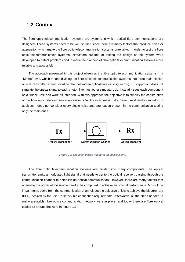
The approach presented in this project observes the fibre optic telecommunication systems in a
“Macro” level, which means dividing the fibre optic telecommunication systems into three main blocks:
optical transmitter, communication channel and an optical receiver (Figure 1.2). This approach does not
simulate the optical signal to each photon like most other simulators do, instead it sees each component
as a “Black Box” and work as intended. With this approach the objective is to simplify the construction
of the fibre optic telecommunication systems for the user, making it a more user-friendly simulator. In
addition, it does not consider every single noise and attenuation present in the communication testing
only the main ones.
Figure 1.2 The main blocks that form an optic system.
The fibre optic telecommunication systems are divided into many components. The optical
transmitter emits a modulated light signal that needs to get to the optical receiver, passing through the
communication channel to establish an optical communication. However, there are many factors that
attenuate the power of the source need to be computed to achieve an optimal performance. Most of the
impairments come from the communication channel, but the objective of it is to achieve the bit error rate
(BER) desired by the user to satisfy his connection requirements. Afterwards, all the steps needed to
make a suitable fibre optics communication network were in place, and today there are fibre optical
cables all around the word in Figure 1.3.

4
Figure 1.3 World map with undersea cable transmission systems until October 2016 [2]
1.3 Objectives and dissertation structure
The aim of this project is to implement a simulator of fibre optic telecommunications systems at a
macro level, the implementation was made using MATLAB® and Simulink. The simulator provides a
simple construction tool in a Simulink library were the components of a fibre optic telecommunications
systems can be added. The different parameters of the components can be altered by the user interface
window that opens by pressing the blocks. The simulator will provide the necessary components to
construct a fibre optic telecommunications system. By constructing this library in Simulink there is always
the possibility of growth, which means that the program was constructed with the intent of allowing
students to add more complexity to the simulator by adding other blocks or functionalities. The
dissertation document is structured as follows:
• In Chapter 2, a theoretical analysis of fibre optic telecommunications systems including the
appllication of each component and phenonmena that occur in the system.
• In Chapter 3, the simulator that was implemented with an explanation on the construction of
the system and each block with a comparision of values with other simulators. This
comparison will be followed by the construction and analysis of a real life project of a fibre
optic telecommunications system with the simulator.
• In Chapter 4, the final conclusions are presented.
5
1.4 State of the art
In this section is divided into two subsections, that explained in which point the technology has been
developed. Since, this project contains two types technology, fibre optics and fibre optic simulator, an
explanation on their development is evaluated separately.
1.4.1 Fibre optics
Since the beginning of time, humans tried to communicate from longer distances and with as much
information as possible. Nevertheless, this would only become possible in the 19th century, with the
development of the electrical telegraph. However, this electrical telegraph had a limited capacity of
sending only 15 words per minute, which was a very primitive system compared to the one used
nowadays [3].
The fibre optic telecommunication systems did not always use silica fibres, this discovery and some
other discoveries led to the technology used nowadays. One of the first findings regarding optical-fibre
communications happened in 1880 with the Photophone, invented by Alexander Graham Bell and
Charles Sumner Tainter. Although this device worked, it had a short range and it did not work without
clear air conditions [4]. The Photophone did not use fibre until 1961 when Charles C. Eaglesfield
proposed the use of a hollow optical pipeline made of reflective pipes. Five years later, a paper was
published by Charles Kao and George Hockham demonstrating that the use of fibreglass could
dramatically decrease if the glass was pure enough, so they proposed that the loss could be reduced
below 20 dB/km, which would be practical for communications [5]. Later in 1970, Corning Glass Works
achieved the first low-loss optical fibre suitable for optical fibre communications, reaching less than 20
dB/km [6].
There has been a growth in the required data to establish a telecommunication. This requirement
has always enticed the necessity for faster and more reliable means of communications. The
development of fibre optic communications can be stated to have started in the 19th century, with the
development of the electrical telegraph. However, this electrical telegraph had a limited capacity of
sending only 15 words per minute, which was a very primitive system compared to the one used
nowadays.
The technology of telecommunications grew exponentially since the electrical telegraph, from
inventions such as the telephone, the radio and the television until today with the use of computers and
the internet. Since the creation of computers and the internet in the 1960s, the bit rate in which
information is transmitted has become increasingly faster.

6
Figure 1.1 shows that the number of users with internet access continuous to rise. Most of these
new connections will already be made from optical fibre cables, and many of the old copper wiring ones
were or will be replaced by fibre optical cables. Figure 1.4 shows an increasing growth in the number of
optical fibre cables used in different countries.
Figure 1.4 Growth in fibre optical cables per country [7]
In many countries, the growth of fibre cables is rising. However, it seems to be less significant in
other countries. For instances in Japan the growth is just 4.82%, but the percentage of coverage is
already 74.1%. This means that there is less growth because the coverage is almost total. On the other
hand, in Australia, the growth was 128.57%, but the percentage of coverage is only 13.4% [8]. The
difference in between these countries is obvious, the growth will directly relate with the total coverage,
but the final conclusion is the same, many countries are investing in this technology. Even if it does not
seem that most countries are investing in this technology by its growth, the reason behind it is because
they have already invested already a lot in this technology and is already implemented.
With the appearance of fibre optic telecommunications, many parameters had to be introduced and
adapted in order to study the phenomena that occur in this kind of telecommunications. An example of
this is the optical signal to noise ratio (OSNR) which was previously analysed as the signal to noise ratio
(SNR). The OSNR represents the ratio between the power of the signal and the noise power in that
signal. This is one of the most important concepts in fibre optic telecommunications because is used to
evaluate the amount of noise in relation to the signal that is received. One of the other parameters
essential for this type of communications is the bit error rate. The BER is the ratio of the received bits
that have been altered due to noise, distortion and interference. Thus, to improve the BER of the
communication channel, the fibre needs to have the smallest distortion as possible. However, even
when using silica fibres, where the losses are as small as 0.2 dB/km, the optical power after 100 km
would be only 1% [9]. Thus, the choice of the components that make the communication channel need
to be studied in order to achieve a good connection and the most cost efficient option.
7
1.4.2 Simulators
The use of fibre optical telecommunications systems simulators is needed to test the viability of the
projected communication, through the selection of the components, the technology, the frequencies and
many other options given by the simulator. Through the simulation of the system, the user is able to
know if his solution is viable and maybe if it is the most cost efficient one. If the simulator provides the
information about the most cost efficient solution, which many of them do, the user can make changes
to save money on the project, or on the maintenance of the system.
The MATLAB® software has the capacity to run numerical models programmed by the user, which
opens many possibilities for further research in many areas. This software will be used for the simulation
of the fibre optic telecommunication systems, and together with Simulink, a block diagram environment
for multi-domain simulation already integrated within MATLAB® [10]. The simulator presented in this
“paper” was created on MATLAB® Simulink since it is a free tool for students. Also, this software is
commonly used in Universities worldwide to test fibre optic telecommunication systems.
However, there are many programs that already provide fibre optic telecommunications systems
simulation, each one of them provides many options and different capacities. Some of them are
companies such as VPIphotonics and Synopsys, these companies provide many solutions for optical
systems. However, these programs are closed platforms that require licenses and cannot be modified
by the user. There also other studies with proposals for a fibre optical telecommunication systems
simulators made by different Universities such as Robochameleon made by Danmarks Tekniske
Universitet (DTU) [11] and also a Master’s dissertation from Instituto Superior de Ciências do Trabalho
e da Empresa - Instituto Universitário de Lisboa (ISCTE-IUL) [12].
VPIphotonics
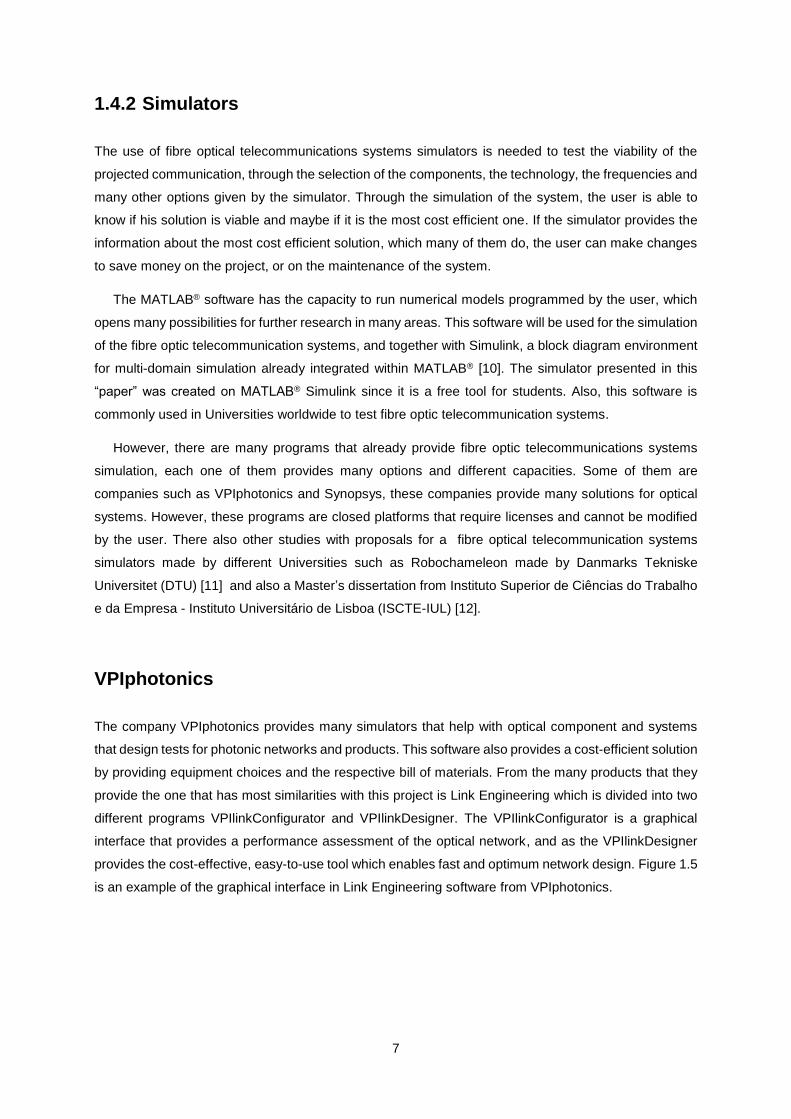
The company VPIphotonics provides many simulators that help with optical component and systems
that design tests for photonic networks and products. This software also provides a cost-efficient solution
by providing equipment choices and the respective bill of materials. From the many products that they
provide the one that has most similarities with this project is Link Engineering which is divided into two
different programs VPIlinkConfigurator and VPIlinkDesigner. The VPIlinkConfigurator is a graphical
interface that provides a performance assessment of the optical network, and as the VPIlinkDesigner
provides the cost-effective, easy-to-use tool which enables fast and optimum network design. Figure 1.5
is an example of the graphical interface in Link Engineering software from VPIphotonics.

8
Figure 1.5 Fibre optic planning tool with four stations using Link Engineering [13]
These simulators are very detailed but require a license to use the software and the user cannot
add new blocks made by him. The amount of possibilities and options that the user has can be very
complex but it can also be confusing for a new user to use the VPIlinkConfigurator that is more complex
than the VPIlinkDesigner. This software includes a MATLAB® interface, which provides a
comprehensive set of additional functionalities for the user, including the ability to integrate and model
equipment models and parts of communication links specified in MATLAB®.
Synopsys
The company Synopsys has a simulator OptSim used to design and simulate optical communication
systems. It uses easy-to-use graphical interface for the user to combine with lab-like measurement
instruments. This software was released in 1998, and engineers use it in academic and industrial
organisations. Figure 1.6 presents an example of an OptSim design and as can be observed it simulates
at the signal propagation level.
Figure 1.6 Application to detect receiver’s sensitivity with OptSim [14]

9
The main features of this program support multiple parameters for a scans-based optimisation. It
has a design tool with multiple engines running in a time and frequency domain. Also, has a MATLAB®
interface in order to facilitate the development of custom user models with m-file language and the
Simulink modelling environment. This means that the software is able to run models added by the user
and the user also has the possibility to work in parallel with the SPICE engine.
Fibre optics telecommunications simulators from other Universities
The projects developed by other Universities such as DTU and ISCTE-IUL showed different approaches
to a fibre optic telecommunication system. Robochameleon the project was developed in MATLAB®
which consists of a framework to build a fibre optic telecommnunication system which can be accessed
by the MATLAB®’s terminal, providing a coherent simulation because it simulates according to the signal
level [11]. However, since this project was not built with Simulink, that is a graphical interface for
MATLAB®, it does not have the capacity to connect different models. Thus, the construction of the fibre
optic telecommunication system using Robochameleon is not very intuitive. In order to work with this
program, there is a necessity to read the user manual to understand how the construction of the fibre
optic telecommunication system is possible. However, the results are very precise with a full graphical
analysis of each component.
The dissertation from ISCTE-IUL developed a planning tool for fibre optic communication system
developed in Java. This simulator also uses Google Maps in order to choose the route of the connection
Figure 1.7. However, the insertion of data to execute mathematical operations is managed in Structured
Query Language (SQL) and PHP: Hypertext Preprocessor (PHP). This project provides a graphical
interface in which is possible to select points on Google Maps using a Google Maps Script and plan a
realistic fibre optic telecommunications system simulation.

10
Figure 1.7 Optical link planning using a Google maps application in simulator from ISCTE-IUL [15]

11
Chapter 2
2. Theoretical Overview
The development of the simulator cannot be made without a theoretical analysis of the system. This
analysis includes the components used in the simulator and the techniques and phenomena that occur
in the system. The construction of the simulator will implement equations and parameters discussed in
this section and a theoretical analysis of the simulator results that can be compared with the theoretical
overview, in order to determine the authenticity of the results provided by the simulator.

12
2.1 Fibre Optic Communications
An explanation of fibre optic communications is the information transmitted from a light source of a
transmitter through an optical fibre that is connected to a receiver. However, in real life conditions, many
fibre optic communications need amplifiers, filters, connectors and other equipment to achieve a fibre
optic communication. The equipment used for a fibre optic communication can bring attenuation and
distortion to the system, so when planning a fibre optical telecommunications system all this attenuations
and distortion need to be taken into account.
Some of the parameters that are necessary to determine many equations in the fibre optic
telecommunications systems are constants such as the speed of light in vacuum. Table 2.1 represents
all the parameters that are predefined as constants in any system and are used in the determination of
some equations in this project. The parameters in Table 2.1 are: the speed of light in vacuum 𝑐 [𝑚/𝑠],
the elementary charge 𝑞[𝐶], the Planck’s constant ℎ[ 𝐽 ∙ 𝑠 ], the Boltzmann constant 𝑘𝑏 [𝐽/𝐾] and the
room temperature 𝑇[𝐾].
Table 2.1 Values of the constants used in fibre optic telecommunications systems
𝑐 [𝑚/𝑠] 𝑞 [𝐶] ℎ [𝐽. 𝑠] 𝑘𝑏 [𝐽/𝐾] 𝑇[𝐾]
299792458 1,601 ∗ 10−19 6.626 ∗ 10−34 1,381 ∗ 10−23 290
The need for amplifiers and other similar equipment is because most fibre optic communications
are made for long-distance communications, since fibre optics is the fastest and more reliable way to
transmit information over long distances. Although this type of equipment inserts distortion and
attenuation to the transition, in many cases is necessary and can be verified by achieving a better OSNR.
In the next sections, all the equipment available in the simulator is explained, as well as the
correspondent attenuation that they bring to the optical signal transmitted in the simulation. The
equipment taken into account were: transmitters, optical fibre, amplifiers, filters and receivers. Note that
the connectors and splices were considered to be a part of the optical fibre.
This technology came to replace the copper cables that were used for long-haul communications.
The advantage of using fibre optical cables instead of copper cables is the possibility to communicate
with a higher bandwidth. Although the cost for a fibre optic communication is higher than copper cables,
the use of fibre optical cables has future-proof capabilities since the market of telecommunications is
requiring higher speed and fidelity. The higher speeds of transmitted information come from the increase
in bandwidth, and the increased fidelity comes from the fact that fibre optic communications need less
signal boosting per meters, so the insertion of noise from regenerators or amplifiers is diminished, and
consequently the signal has a higher fidelity. One of the basic concepts of fibre optic communications
that need to be taken into account is the relation between the signals wavelength and the signal
frequency. The relation between these two parameters is demonstrated in Equation (2.1), where the
parameters are wavelength 𝜆, frequency 𝑣 and 𝑐 is the speed of light in vacuum.

13
𝜆 =𝑐
𝑣 (2.1)
2.2 Optical Transmitter
The light source in a fibre optic communication is generated in a transmitter that converts an electric
signal into a light signal. The optical transmitter contains a light source that transmits the light signal
through the fibre. The transmitter can modulate the signal internally or externally. The use of internal
modulation has some disadvantages related to the signal transmission. Since in fibre optic
communications the emitted power only reproduces an electrical current if the variations of current are
reasonably slow. The necessity for slow variations is due to the emission of photons that can replicate
the exact variations in the electrical current. Thus, this happens only if the bandwidth of the laser is
similar or higher than the transmitted bit-rate. Ultimately, the necessity of slow variations in the current
will limit the use of higher bitrates with internal modulation, with bit-rate higher than 10[𝐺𝑏𝑖𝑡/𝑠] [16]. With
external modulation, the chirp parameter 𝐶 inserted by the transmitter is zero, the chirp parameter is
related to the frequency chirp imposed on signal. The signal can be chirped meaning that the carrier
frequency is changing with time, broadening the signal and leading to power penalties of the received
power due to pulse broadening.
The bit-rate for a signal Synchronous Transport Module (STM) level-N is given by the Equation
(2.2) [17]. STM is the recommended Synchronous Digital Hierarchy (SDH) for fibre optic networks by
the International Telecommunication Union (ITU-T).
B𝑆𝑇𝑀−𝑁 = N×155.52×10
6bit/s
(2.2)
Another problem when using internal modulation is the fact that the lowest level of current has to
be higher than the threshold current. The threshold current is the needed current that the laser needs
to operate. The solution to this problem is to use levels of current above the threshold current, which will
generate that the current for the logic level “0” higher than zero. Thus, by having a current higher than
zero results in a new parameter to quantify how far is the half power from the minimum power, being
the logic level “0” equal to zero. ITU-T defined this parameter in the recommendation G.957, designated
by extinction ratio 𝑅𝑒𝑥𝑡.
The extinction ratio influences the receiver sensitivity because the power emitted during 0 bits due
to spontaneous emission can be a significant fraction, detailed moreover in Section 2.4.1. The mean
power of the logic level “0” and “1” being respectively 𝑃0 and 𝑃1. The extinction ratio is given by the
Equation (2.3) [9]. Note that for simplification normally 𝑟𝑒𝑥𝑡 is represented as 𝑟 = 1/𝑟𝑒𝑥𝑡, and by the ITU-
T Rec. G.957 the minimum value for the extinction ration is 𝑅𝑒𝑥𝑡 = 8.2[𝑑𝐵]or 𝑟𝑒𝑥𝑡=6.6.
𝑟𝑒𝑥𝑡 =𝑝1[𝑊]
𝑝0[𝑊] (2.3)
14
The emitted power of the light source is one of the influential parameter. This parameter can be
limited by nonlinear effects and other parameters. However, the maximum power can be limited also by
cost efficiency, since the more power the system emits the more expensive will be to maintain it.
However, if not enough power is used to compensate for all the attenuations of the system, the receiver
might not receive a detectable signal. This parameter can be measured and is the receiver sensitivity,
this issue will be discussed further in Section 2.4. Another influential parameter of the optical transmitter
is the root mean square width of the source spectrum 𝜎𝜆 [𝑚]. In a normal distribution, the full width at
half maximum or ∆𝑣 is given by the Equation (2.4) [16].
𝜎𝜆 =∆𝜆
2√2 ∙ ln (2) (2.4)
The linewidth ∆𝜆 in [𝑚], can be determined with the Equation (2.5), where the nominal wavelength is
represented by 𝜆0, speed of light in vacuum 𝑐 and linewidth of the laser ∆𝑣 in [𝐻𝑧].
∆𝜆 =∆𝑣 ∙ 𝑐
𝜆02 (2.5)
However, if the linewidth of the transmitter is small, normally smaller than ∆𝜆 << 1 [𝑛𝑚], then the
root mean square width of the source spectrum will not depend on the linewidth of the transmitter laser.
The maximum linewidth will be determined with the signal’s bit rate, thus, in order to determine the
linewidth used in Equation (2.4) the maximum linewidth calculated with Equation (2.6) is used instead,
where the parameter 𝐵 is the bit-rate of the system.
∆𝜆𝑀 =𝐵
𝜆02 𝑐
(2.6)
The transmitter also sets the number of channels using wavelength-division multiplexing technique,
where WDM multiple signals can be carried through a single fibre using different wavelengths. With
more than one channel there will be crosstalk produced in the filters that are analysed in Section 2.6.
The frequency for each channel is determined by the Equation (2.7), the parameters in this equation are
the frequency of nth channel 𝑣𝑛, the frequency of the first channel 𝑣1 and channel spacing ∆𝑣𝑐ℎ.
𝑣𝑛 = 𝑣1 + (𝑛 − 1)∆𝑣𝑐ℎ (2.7)
The channel spacing is the gap between two neighbouring frequency, the space between two signals
can lead to crosstalk if the space is not big enough, moreover in Section 2.6.1. There are also power
penalties that the system will have to take into account directly related with the optical transmitter. This
power penalties are related with the mode-partition noise and relative intensity noise, moreover Section
2.7
2.3 Optical Fibre
The optical fibre is the communication channel of a fibre optical telecommunications system, the optical
fibre is made, in most cases, of two layers of a transparent material that can be either plastic or glass.
The reason for it, they have the lowest attenuation per kilometre with the capability to transmit optical

15
signals. The two layer are set within another to form an inner core and an outer cladding that can be
observed in Figure 2.1. The transmission can be achieved within the fibre by transmitting light through
the inner core and reflecting it through the fibre. This phenomenon is achieved by transmitting the optical
signal throughout the fibre and propagating it due to the inner core having a refractive index 𝑛1 that is
higher than the refractive index of the cladding 𝑛2 represented in Figure 2.1. The Snell’s law, Equation
(2.8), is the principle behind the refraction within the fibre, where ∅1 and ∅2 are the angle of incidence
and refraction, respectively. With this principle, it is possible to predict the total internal reflection in the
core of the fibre. The total internal reflection is the phenomenon that provides the propagation of the
light through the fibre.
𝑛1 sin(∅1) = 𝑛2 sin(∅2) (2.8)
Normally optical fibres are exclusively made of glass, mainly silica (SiO2). However, normally the
silica fibres are not pure silica, since pure silica fibres are usually not suitable for most fibre optical
telecommunications systems, so some dopants are added such as GeO2 and P2O5. Even with low
attenuation per kilometre, the optical fibre is the main source of attenuation in a fibre optic
communication discussed in Section 2.3.3. Also, presents performance limitations of a fibre optical
telecommunications system with fibre dispersion by broadening optical pulses inside the fibre discussed
in Section 2.3.4. For means of simplification, the simulator also has the attenuation generated by the
connectors and splices, which are devices used to connect the fibres with connectors and the fibre with
the other devices with splices. This attenuation will be inserted with fibre losses in Section 2.3.3.
Figure 2.1 Optical fibre structure, adapted from [16]
There are many types of fibres currently in use, their functions can go from submarine cables as
shown in Figure 1.3, aerial suspended on poles and long-haul applications. Following the ITU-T
recommendations, which is the global standardisation organisation for telecommunication systems. In
this project only two types of optical fibres were used. The nondispersion-shifted fibre (NDSF) also
known as the standard single-mode optical fibre (SMF) and the non-zero dispersion-shifted fibre
(NZDSF), also referred as ITU-T G.652 and ITU-T G.655 respectively. These types of fibres were

16
designed to overcome different problems within fibre optical telecommunications system and are
explained in the following sections. Although, these two types of fibres were the only ones introduced
this means that they were the only ones with already inserted standard values, following an example for
each fibre. However, the users can always customise each block to replicate another type of fibre.
There are also some other important parameters of the fibre that are related to nonlinear effects
that will be analysed in Section 2.3.5. The parameters that will directly influence the nonlinear effects
are the effective core area of the fibre 𝐴𝑒𝑓𝑓 = 𝜋𝑤2. Where the 𝑤 is the field radius also referred as spot
size. The effective core area determines how tightly the light is constrained within the core. It will affect
directly the nonlinear effects in the transmission, by restraining the power in the system for a smaller
effective core area.
2.3.1 Nondispersion-shifted fibre (ITU-T G.652)
The standard ITU-T G.652 is the most used optical fibre in a telecommunications system. This type of
fibre optimised to work with wavelengths in the 1310 [𝑛𝑚] band, which comes from having its zero-
dispersion wavelength at 1310 [𝑛𝑚] [18]. The zero-dispersion wavelength is where the material
dispersion and waveguide dispersion cancel each other. Although this type of fibre is optimized to work
in with wavelengths in the 1310 [𝑛𝑚] band, it can also operate in the wavelengths in the 1550 [𝑛𝑚]
band. A typical attenuation parameter for this type of fibre is 0.2𝑑𝐵/𝑘𝑚 and a chromatic dispersion at
17𝑝𝑠/𝑛𝑚/𝑘𝑚 at 1550 𝑛𝑚.
In this project, there is a possibility to introduce the attenuation of the fibre if the user wants to use
a specific value. However, if no value is introduced the simulator will use the values of a standard
Corning SMF-28 fibre that is a ITU-T G.652 taken from its datasheet [19].
2.3.2 Non-zero dispersion-shifted fibre (ITU-T G.655)
The limiting factor for a fibre link in long-haul systems is the fibre dispersion. The limiting factor is not
the power since the use of amplifiers to keep the power of the signal throughout the system. However,
the amplifier noise often forces the need to increase the channel power in order to keep a high OSNR.
Ultimately this increases the accumulation of the nonlinear effects of the fibre ends up limiting the length
of the system. So, the need to develop a type of fibre such as NZDSF that mitigates these nonlinear
characteristics was necessary. This type of fibre surpasses these effects by having a bigger effective
core area 𝐴𝑒𝑓𝑓, that is demonstrated in Section 2.3.5, which will diminish the restrictions from the
nonlinear effects. Also, the zero-dispersion wavelength is outside of the 1550 [𝑛𝑚] band. The ITU-T
G.655 achieves a small chromatic dispersion at 1550 [𝑛𝑚], usually at 4.5𝑝𝑠/𝑛𝑚/𝑘𝑚 and the attenuation
parameter usually at 0.2𝑑𝐵/𝑘𝑚 .

17
The fibre ITU-T G.655 is divided into two families which the values for the chromatic dispersion
drop before or after 1550 [𝑛𝑚], which are called NZD+ and NZD- respectively. In this project, there is
also a possibility to introduce the attenuation of the fibre NZDSF if the user wants to use a specific value.
However, if no value is introduced the simulator will use the values of a standard Corning LEAF fibre
that is a ITU-T G.652 taken from its datasheet [20]. With the information taken from the datasheet, Figure
2.2 was reconstructed and inserted in the simulator for a standard ITU-T G.652 fibre.
Figure 2.2 Variation of the attenuation of the through the wavelength of Corning LEAF fibre [20]
2.3.3 Fibre Losses
The fibre losses reduce the power of the signal reaching the receiver, this attenuation 𝐴𝑇[𝑑𝐵] can be
measured with the attenuation coefficient 𝛼 [𝑑𝐵/𝑘𝑚] that takes into account the material absorption and
other sources of power attenuation in the fibre. This parameter can also be represented in Neper per
kilometre 𝛼𝑛 [𝑁𝑝/𝑘𝑚], and it can be converted with the Equation (2.9) [16] .
𝛼[𝑑𝐵/𝑘𝑚] = 4.343𝛼𝑛[𝑁𝑝/𝑘𝑚] (2.9)
The attenuation coefficient changes with the signal wavelength, as showed in the Figure 2.2 [20].
Another power reduction parameter is the attenuation from splices and connectors of the fibre, 𝐴𝑆 and
𝐴𝐶 respectively, this splices and connectors are necessary to form the fibre link. With Equation (2.10)
[15], the fibre losses or attenuation of the fibre can be calculated, where 𝐿𝑇𝑜𝑡𝑎𝑙 stands for the total length
of the fibre in [𝑘𝑚], 𝑁𝑆 to the number of splices in the link and 𝑁𝐶 the number of connectors.
𝐴𝑇 = 𝛼 ∙ 𝐿𝑇𝑜𝑡𝑎𝑙 + 𝑁𝑆 ∙ 𝐴𝑆 + 𝑁𝐶 ∙ 𝐴𝐶 (2.10)
2.3.4 Fibre Dispersion
The fibre dispersion also known as chromatic dispersion causes pulse broadening. Thus, the spectral
components of the pulse travel at slightly different group velocities. By the pulses travelling at different
velocities will result in intersymbol interference between the receiving pulses increasing the bit errors at
the receiver, represented in Figure 2.3.

18
Figure 2.3 Representation of pulse broadening in the fibre link, adapted from [12]
The fibre dispersion is divided into two types of dispersion material dispersion and waveguide
dispersion. Material dispersion results from the variation of the inner core refractive index with the
wavelength. Waveguide dispersion results from some of the optical power, inserted in a SMF, escaping
from the inner core and keep propagating in the cladding. This optical power travels at faster speeds
than the inner core resulting in pulse broadening. The both types of dispersion are considered in the
Equation (2.11) [16] referring to the fibre chromatic dispersion.
𝐷𝜆 = 𝐷𝑟 + 𝑆𝑟 ∙ (𝜆 − 𝜆0) (2.11)
In Equation (2.11) the parameters are the central wavelength 𝜆0, the wavelength of the signal 𝜆,
the dispersion slope since 𝑆𝑟 and the dispersion parameter 𝐷𝑟. The dispersion parameter 𝐷𝑟 [𝑝𝑠/(𝑘𝑚 ∙
𝑛𝑚)] can be calculated with the Equation (2.12) [9], where the speed of light in vacuum is represented
by 𝑐 and 𝛽2 represents group velocity dispersion parameter.
𝐷𝑟 = −2𝜋 ∙ 𝑐 ∙ 𝛽2
𝜆2 (2.12)
The parameter 𝑆𝑟 is the differential-dispersion parameter or dispersion slope since 𝑆𝑟 = 𝑑𝐷/𝑑𝜆
resulting in the Equation (2.13) [9], with 𝛽3 representing the third-order dispersion parameter.
𝑆𝑟 = (2𝜋 ∙ 𝑐
𝜆2)2
∙ 𝛽3 + (4𝜋 ∙ 𝑐
𝜆3) ∙ 𝛽2 (2.13)
2.3.5 Nonlinear Effects
The assumption that is made by despising the nonlinear effects is that within the optical fibre the optical
signals will not interact with each other. Also, it is assumed that these properties do not directly affect
directly the optical signal power transmitted to the fibre. Although in NZDSF fibres there were
19
improvements in order to have the smallest the nonlinear coefficient as possible, these effects cannot
be despised when planning a fibre optic telecommunication system. Also, if the systems contain optical
amplifiers, nonlinear effects may accumulate over long distances, due to the nonlinear effects
dependence on the fibre length. However, most nonlinear effects occur early in the fibre since in longer
ranges the signal will be attenuated. The nonlinear effects are divided into two types stimulated light
scattering and nonlinear phase modulation.
2.3.5.1 Stimulated Light Scattering
The stimulated light scattering is divided into two types stimulated Brillouin scattering (SBS) and
stimulated Raman scattering (SRS), these effects are explained in the following sections.
Stimulated Brillouin scattering
The acoustic vibration in the optical fibre will interact with the light signal, transmitted in the fibre, causing
a nonlinear effect called stimulated Brillouin scattering. This effect causes the down-conversion of the
light signal, causing the appearance of phonons from the released energy. Phonons are the collective
excitation of atoms that form the fibre, this phenomenon will cause an acoustical pressure wave, referred
to as electrostriction, which travels through the fibre at the speed of sound following the same direction
of the light signal. The propagation of the electrostriction will periodically change the refractive index of
the fibre since it depends on the density of the fibre, with the biggest influence being the variation in the
core diameter. This nonlinear effect will affect the maximum threshold power that can be determined by
the Equation (2.14) [9].
𝑃𝑡ℎ ≈21 ∙ 𝐴𝑒𝑓𝑓
𝑔𝐵 ∙ 𝐿𝑒𝑓𝑓 (2.14)
With the Equation (2.14), it can be observed that this constraint due to SBS will be affected by the
fibre dimensions with the effective core area 𝐴𝑒𝑓𝑓, the SBS gain 𝑔𝐵 ≈ 5×10⁻¹¹[𝑚/𝑊] for silica fibres
and the effective interaction length 𝐿𝑒𝑓𝑓 that can be calculated with the Equation (2.15) [9].
𝐿𝑒𝑓𝑓 =1 − exp(−𝛼𝐿)
𝛼
(2.15)
Stimulated Raman scattering
The photons of a light signal transmit simultaneously through the fibre if a light signal has a lower energy
and frequency can be stimulated by another light signal with higher frequency and energy. This
phenomenon can result in the nonlinear scattering of light photons, this effect is called stimulated
scattering effect. This effect causes the downshifting of the frequency, causing the appearance of
phonons from the released energy, phonons as it was referred in the previous section are the collective
excitation of atoms that form the fibre, this phenomenon will shift the frequency of an amount equal to

20
the molecular vibration frequency also called Stokes shift. The effect of SRS in a fibre optic
telecommunications system is the reduction of maximum threshold power inserted in the fibre. The
maximum threshold power limited by the SRS can be determined with the Equation (2.16) [9], where
the SRS gain 𝑔𝑅 ≈ 6×10⁻¹³[𝑚/𝑊] at 1550 [𝑛𝑚].
𝑃𝑡ℎ ≈16 ∙ 𝐴𝑒𝑓𝑓
𝑔𝑅 ∙ 𝐿𝑒𝑓𝑓 (2.16)
2.3.5.2 Nonlinear phase modulation
The nonlinear phase modulation is divided into three types: four-wave mixing (FWM), self-phase
modulation (SPM) and cross-phase modulation (XPM). These effects are explained in the following
sections.
Self-phase modulation
By applying a light source to a material an electric field is created, and it will cause variations in the
refraction index of that material, this phenomenon is called Kerr electro-optic effect. These variations in
the refraction index of the fibre will result in variations in the phase of the light, this effect is called self-
phase modulation. The Kerr effect varies with the square of the electric field. Thus, reducing the
transmission power, the electric field will be reduced as well. First and foremost, the nonlinear parameter
must be determined resorting to the Equation (2.17) [9], where 𝑛2 [𝑚2/𝑊] is the numerical value related
to dopants inside the core of silica fibres.
𝛾 =2𝜋𝑛2
2
𝜆 ∙ 𝐴𝑒𝑓𝑓
(2.17)
The important part to observe in Equation (2.17) is that the nonlinear parameter directly related
with 𝐴𝑒𝑓𝑓. Once again proving that NZDSF fibres have a bigger 𝐴𝑒𝑓𝑓 will decrease the nonlinear effects.
Also, it fluctuates with the wavelength of the signal 𝜆.The Phase shift produced by SPM is given by the
Equation (2.18) [9].
𝜙𝑁𝐿 = 𝛾 ∙ 𝑃𝑖𝑛 ∙ 𝐿𝑒𝑓𝑓 (2.18)
In order to reduce the impact of SPM from the phase shift must be 𝜙𝑁𝐿 ≪ 1. Thus, the value
maximum accepted value for the phase shift was considered 𝜙𝑁𝐿 = 0.1. Solving the Equation (2.18) in
order of 𝑃𝑖𝑛 the maximum power that can be inserted in the fibre can be determined with the Equation
(2.19), where 𝑁𝐴 is the number of amplifiers, since the phase shift will accumulate over multiple
amplifiers.
𝑃𝑖𝑛 <0.1
𝛾 ∙ 𝐿𝑒𝑓𝑓 ∙ 𝑁𝐴 (2.19)

21
Cross-phase modulation
The crosstalk generated in WDM technique also creates a variation of the transmitted power in the fibre.
Thus, the crosstalk power insertion with a WDM system will induce limitations of the insertion power in
the fibre. Since the nonlinear shift it not only depends on a specified channel but also on the power of
other channels. This variation in the phase shift can be determined by the Equation (2.20) [9] for the 𝑗th
channel.
𝜙𝑗𝑁𝐿 = 𝛾 ∙ 𝐿𝑒𝑓𝑓 ∙ (𝑃𝑗 + 2 ∑ 𝑃𝑚
𝑚≠𝑗
) (2.20)
In order to get the maximum value for 𝑃𝑗, as in SPM, the value for the phase shift must be 𝜙𝑁𝐿 =
0.1. Thus, by solving the Equation (2.20) in order of 𝑃𝑗 the Equation (2.21) is obtained.
𝑃𝑗 <0.1
𝛾 ∙ 𝐿𝑒𝑓𝑓 ∙ 𝑁𝐴− 2 ∑ 𝑃𝑚
𝑚≠𝑗
(2.21)
Four-wave mixing
In a link with WDM, channels with different wavelengths can mix forming a new wave with a different
frequency. This effect is known as four-wave mixing, in order to prevent this effect from occurring the
signal power is limited. This effect is one of the major significant degrading effects in WDM in a fibre
optic telecommunications system. However, the limitation factor needs some parameters that imply the
use of the real simulation of the signal. Thus, due to the complexity of implementing this nonlinear effect,
this effect was not implemented in the program.
2.4 Optical Receiver
The optical receiver is the opposite end of the optical transmitter line, the function of an optical receiver
is to detect the optical signal and converting it into an electrical signal, by interpreting the information
received from the optical signal. The detection of the optical signal is possible due to a photodetector
inserted within the optical receiver. The photodetector is converting the detected light that shines upon
him, into an electrical signal. The two main types of photodiodes used are an avalanche photodiode and
a p-i-n photodiode.
The difference between the APD and PIN receiver is that the APD receiver has an amplification of
the signal 𝑀𝐴𝑃𝐷 within the receiver. However, in PIN receiver normally the same parameter is usually
𝑀𝑝𝑖𝑛 = 1, which means that there is no amplification of the signal. This will result in the APD receiver
having an extra noise factor 𝐹𝐴 in comparison with the PIN receiver, but APD receivers supporting less
power at the end of the photodetector since the signal is amplified after the optical to electrical signal
conversion. Although this can be proved to result in a better communication, for this reason both
solutions are presented to the user in the simulation.

22
The ability to detect the optical signal received from the optical receiver can be measured, this
parameter is called receiver sensitivity. The receiver sensitivity is a very important parameter since if
the optical power that reaches the optical receiver is lower than the receiver sensitivity. The optical
receiver will not detect it, moreover in the following sections. Another parameter that of the receiver that
should be taken into account in a fibre optic telecommunication system is the overload power of the
receiver. This parameter differs from each receiver and is normally presented in the datasheet of the
receivers, if the received power surpasses this parameter the receiver can get permanent damage.
2.4.1 Receiver Sensitivity
The sensitivity of a receiver is the minimum input signal of the receiver. In order to determine the receiver
sensitivity, the BER required by the receiver must be determined. The BER is defined as the probability
of bit errors per time unit, the number of bit errors is the number of bits received that have been altered
due to distortion, interference and noise. The receiver sensitivity in order to operate at a specified
probability of BER requires a minimum average received power 𝑃�̅�. Since, the bit misinterpretation
corresponding to “1” or “0” in a bit stream can be both included by defining the error probability as the
Equation (2.22) [9].
𝐵𝐸𝑅 = 𝑝(1)𝑃 (0
1) + 𝑝(0)𝑃 (
1
0) (2.22)
The bits with the logical level “1” and “0” have the same probability to occur so 𝑝(1) = 𝑝(0) = 0.5
and the BER probability can be determined with Equation (2.23) [9] that depends only on the 𝑄
parameter. The parameter Q is the ration between a signal current mean difference and a total noise
current drift pattern.
𝐵𝐸𝑅 =1
2𝑒𝑟𝑓𝑐 (
𝑄
√2) (2.23)
Noting that in the Equation (2.23) 𝑒𝑟𝑓𝑐 stands for the complementary error function that is given
by the Equation (2.24).
𝑒𝑟𝑓𝑐(𝑥) =2
√𝜋∫ 𝑒−𝑦
2𝑑𝑦
∞
𝑥
(2.24)
Solving the equation in order to the parameter 𝑄 the Equation (2.23), since there is a requirement
to have specific 𝐵𝐸𝑅 in order to maintain reliable simulation, the Equation (2.25) is obtained.
𝑄 = √2 ∙ 𝑒𝑟𝑓𝑐−1(2 ∙ 𝐵𝐸𝑅) (2.25)
With the parameter 𝑄 the required minimum average received power 𝑝�̅� can be obtain for a given
value of 𝑄 since both equations are correlated with the Equation (2.26) [9], where 𝜎𝑆 is the shot-noise,
𝜎𝑇 is the thermal noise, 𝑀 is the gain of the receiver and 𝑅 the responsivity of the receiver.
𝑄 =2 ∙ 𝑀 ∙ 𝑅 ∙ 𝑝�̅�
√𝜎𝑆2 + 𝜎𝑇
2 + 𝜎𝑇 (2.26)

23
The thermal noise and the shot noise cause fluctuations in the current. The shot noise is generated
by the fact that the electrical current in the receiver is a stream of electrons that is generated at random
times. The thermal noise occurs due to the fluctuations of current generated by a random thermal motion
of electrons in a resistor. This noise is equal for the APD and PIN receivers. On the contrary, the shot-
noise only affects ADP receivers since the PIN receivers normally do not have a gain. The shot-noise
can be determined with the Equation (2.27) [9].
𝜎𝑆 = √(2 ∙ 𝑝�̅�) ∙ 2 ∙ 𝑅 ∙ 𝑞 ∙ 𝐹𝐴 ∙ ∆𝑓 ∙ 𝑀2
(2.27)
With the Equation (2.26) and (2.27) resolving in order of 𝑝�̅� then Equation (2.28) [9] is obtained.
This formula is the receiver sensitivity for whether PIN receivers and APD receivers.
𝑝�̅� =𝑄
𝑅(𝑞 ∙ 𝐹𝐴 ∙ 𝑄 ∙ ∆𝑓 +
𝜎𝑇𝑀)
(2.28)
In order to solve Equation (2.28), there is a need to determine some parameters such the
responsivity of the receiver 𝑅. The responsivity of the receiver is the ratio between the output current of
the photodetector and the optical power received, this parameter is sometimes characterized as the
performance of the receiver. This parameter can be determines with the Equation (2.29) [9], this
equation can be determined knowing the elementary charge 𝑞[𝐶], the quantum efficiency of the receiver
𝜂 that can take values from [0,1], the Planck’s constant ℎ[ 𝐽 ∙ 𝑠 ] and the frequency of the optical signal
𝑣 [𝐻𝑧], that can be determined with the Equation (2.1).
𝑅 =𝑞 ∙ 𝜂
ℎ ∙ 𝑣
(2.29)
Another parameter needed to determine the Equation (2.28), is the excess noise factor 𝐹𝐴 that can
be calculated with the Equation (2.30) [9], where 𝑘𝐴 is the ionization-coefficient ratio and 𝑀 is the gain
of the receiver, these parameters depend on the type of receiver if it is an APD or a PIN receiver.
𝐹𝐴 = 𝑘𝐴 ∙ 𝑀 + (1 − 𝑘𝐴) ∙ (2 −1
𝑀)
(2.30)
Normally in PIN receivers 𝑀𝑝𝑖𝑛 = 1 and 𝑘𝐴𝑝𝑖𝑛 = 0 resulting in the 𝐹𝐴𝑝𝑖𝑛 = 1 . On the other hand, the
ionization-coefficient ratio for APD receiver is higher being in the range 0 < 𝑘𝐴 < 1 and the gain of the
receiver for APD is also higher enhancing the signal that should improve the SNR. The gain of the APD
receiver 𝑀𝐴𝑃𝐷 is given by the Equation (2.31) [9] and should be at least 𝑀𝐴𝑃𝐷 > 10.
𝑀𝐴𝑃𝐷 =1
√𝑘𝐴∙ √
𝜎𝑇𝑄 ∙ 𝑞 ∙ ∆𝑓
+ 𝑘𝐴 − 1 (2.31)
In order to determine if the PIN receiver or the APD receiver is better for the optical communication
in study, the simulator will evaluate which receiver has the biggest sensitivity 𝑃�̅�. The best receiver will
be the one that has the lowest 𝑃�̅� because the minimum average received power for specified value will
require less value for the same performance. Also, a lower 𝑃�̅� will provide a lower optical signal to noise
ratio, moreover Section 2.8.

24
The thermal noise or Johnson-Nyquist noise 𝜎𝑇 , in the Equation (2.32) [9], is the noise generated
by the thermal motion of electrons inside conductors. The formula used to determine this noise can be
determined by considering the room temperature 𝑇 = 290 𝐾; the Boltzmann constant 𝑘𝐵 [𝐽/𝐾]; the
resistor 𝑅𝐿 = 1𝑘𝛺 and the amplifier noise figure 𝑓𝑛 is in linear and not in [dB].
𝜎𝑇 = √4𝑘𝐵𝑇
𝑅𝐿𝑓𝑛∆𝑓
(2.32)
The last parameter that was not presented so far to solve Equation (2.32), is the effective noise
bandwidth of the receiver ∆𝑓. This parameter depends on the receiver design. However, in this simulator
the standard value of this parameter was determined in Equation (2.33).
∆𝑓 = 0.7 ∙ 𝐵 (2.33)
The amplifier noise figure 𝑓𝑛 in case the connection has several amplifiers can be determined with
the Equation (2.34) [9], this equation follows the Friis formula, where 𝑓𝑛𝑖 is the linear noise figure of the
amplifier 𝑖, and 𝑔𝑖−1 is the linear gain of the amplifier 𝑖 − 1.
𝑓𝑛 = 𝑓𝑛1 +
𝑓𝑛2 − 1
𝑔1+𝑓𝑛3 − 1
𝑔1 ∙ 𝑔2+
𝑓𝑛4 − 1
𝑔1 ∙ 𝑔2 ∙ 𝑔3+⋯+
𝑓𝑛𝑖 − 1
𝑔1 ∙ 𝑔2 ∙ 𝑔3 ∙ … ∙ 𝑔𝑖−1
(2.34)
2.4.2 Receiver Sensitivity with Preamplification
In a fibre optical telecommunication system, the amplifier can be inserted anywhere between the optical
transmitter and the optical receiver. One technique when using amplification in the fibre is positioning
the optical amplifier before the optical receiver is preamplification, demonstrated in Figure 2.4. This
technic can have significant improvements in the system by improving the optical signal to noise ratio.
This issue is further discussed in Section 2.8. The use of preamplification improves the sensitivity of the
optical receiver, this improvement comes from the amplification of the signal before reaching the
receiver. However, the thermal noise becomes negligible comparing it to the noise induced by the
preamplifier.
Figure 2.4 Demonstration of Preamplification technic

25
With this technique, the use of an optical filter is imperative in order to reduce some of the amplifier
noise. Since, a phenomenon called amplified spontaneous emission (ASE) occurs in the amplifier,
further discussion of this issue in Section 2.5, an optical filter is used between them, in order to minimise
the noise induced by the optical amplifier, as it can be observed in Figure 2.4. The sensitivity of the
receiver maintains the same definition from Section 2.4.1. However, the equation to determine it is
changed due to the predominant noise factor with preamplification ceases to be the thermal noise and
becomes the noise induced by the preamplifier. This change can be observed with the Equation(2.35)
[9] that is used to determine the receiver sensitivity using this technique.
𝑝�̅� = ℎ ∙ 𝑣 ∙ 𝐹𝑛 ∙ ∆𝑓 ∙ 𝑄
(
𝐹𝐴 ∙ 𝑄 ∙ +
√∆𝑣𝑜𝑝𝑡∆𝑓
𝑀
)
(2.35)
In order to determine the Equation (2.35), the only parameter that has not been presented yet is
the bandwidth of the optical filter ∆𝑣𝑜𝑝𝑡, if a filter is not used than ∆𝑣𝑜𝑝𝑡 will be the bandwidth of the
amplifier.
2.4.3 Sensitivity Degradation
The sensitivity of the receiver in Section 2.4.1 only takes into account the receiver noise, if the optical
signal received is an ideal stream such as optical pulse with a constant energy for 1 bits and no energy
for 0 bits. For a realistic optical signal, the noise added at optical amplifiers per example and degradation
through the fibre link results in the minimum average optical power required 𝑝�̅� increasing.
Degradation of the sensitivity due to the extinction ratio
In most transmitters, some power is still emitted by 0 bits, this means that they still emit some power in
their off state. In the case of semiconductor lasers, the ratio between the off-state power 𝑃0 and the on-
state power 𝑃1 is called extinction ratio 𝑅𝑒𝑥𝑡. The 𝑅𝑒𝑥𝑡 can influence the receiver sensitivity, because of
its relation with the power emitted during 0 bits, as it was referred in Section 2.2. This phenomenon
degrades the receiver sensitivity, by analysing the definition proposed by ITU-T Rec. G.957 it is possible
to determined that the optimal extinction ratio is 𝑟𝑒𝑥𝑡 = ∞. This optimal extinction ratio will generate the
lowest sensitivity degradation. This is also possible to be verified by combining the definition of the mean
receiver sensitivity, given by Equation (2.36) [9] and Equation (2.3).
𝑝�̅� =(𝑝0 + 𝑝1)
2
(2.36)
On the other hand, as it was discussed in Section 2.4 it is also given by Equation (2.26) resulting
in the Equation (2.38) when combining the Equations (2.37) and (2.36).
26
𝑄𝑒𝑥 =(1 − 𝑟)
(1 + 𝑟)
2 ∙ 𝑀 ∙ 𝑅 ∙ 𝑝�̅�
√𝜎𝑆2 + 𝜎𝑇
2 + 𝜎𝑇 (2.38)
It can be observed that the sensitivity generated with extinction ratio Equation (2.28) will be different
than in the Equation (2.38) if 𝑟 > 0. Resolving the Equation (2.38) in order of 𝑝�̅� the Equation (2.39)is
obtained.
𝑝�̅�𝑒𝑥 =(1 + 𝑟)
(1 − 𝑟)(𝑞 ∙ 𝐹𝐴 ∙ 𝑄 ∙ ∆𝑓 +
𝜎𝑇𝑀) (2.39)
The power penalty induced by the extinction ratio is given by the ratio between 𝑝�̅�𝑒𝑥 and 𝑝�̅�
represented in the Equation (2.40).
𝛿𝑒𝑥 = 10 ∙ 𝑙𝑜𝑔10 (𝑝�̅�𝑒𝑥𝑝�̅�) (2.40)
However, since the formulas are similar, the only difference is the extinction ratio that can also be
simplified using the Equation (2.41). So, analysing the equation is possible to confirm that the optimal
extinction ratio is 𝑟𝑒𝑥𝑡 = ∞, resulting in 𝛿𝑒𝑥 = 0[𝑑𝐵] having no degradation to the sensitivity whatsoever.
𝛿𝑒𝑥 = 10 ∙ 𝑙𝑜𝑔10 ((1 + 𝑟)
(1 − 𝑟)) (2.41)
Degradation of the sensitivity due to the Timing Jitter
One of the assumptions of Section 2.4.1 is that the sample of the signal is at the peak of the voltage
pulse. However, the sample is determined by the clock-recovery circuit since the input for this circuit
comes from a noisy nature it results in a fluctuation. This phenomenon is called timing jitter and it
ultimately causes a degradation in the receiver sensitivity. The degradation caused by the timing jitter
to the receiver sensitivity can be determined by the Equation (2.42) [9].
𝛿𝑗 = 10 ∙ 𝑙𝑜𝑔10 (1 − 𝑏/2
(1 − 𝑏/2)2 − 𝑄2𝑏2/2) (2.42)
In the Equation (2.42) the parameter 𝑄 can be determined with the Equation (2.26) and the constant
𝑏 can be determined with the Equation (2.43) [9].
𝑏 = (4𝜋2
3− 8) ∙ (𝐵 ∙ 𝜏𝑗)
2
(2.43)
The parameters in the Equation (2.43) are 𝐵 that stands for the bit-rate of the system and 𝜏𝑗 is the
root-mean-square value of the timing jitter.

27
Degradation of the sensitivity due to the Intensity Noise
The light emitted by a transmitter has power fluctuations, these fluctuations are referred as intensity
noise. These fluctuations cause a variation in the signal power and in order to take into account this
phenomenon in the system, a degradation of the sensitivity s taken into account. This degradation can
be determined by the Equation (2.44) [9].
𝛿𝐼 = −10 ∙ 𝑙𝑜𝑔10(1 − 𝑟𝐼
2𝑄2) (2.44)
The parameters from the Equation (2.44) are the parameter 𝑄 from the Equation (2.26) and the
parameter for the intensity noise 𝑟𝐼. This particular parameter can be determined with the Equation (2.45)
[9].
𝑟𝐼2 = 2 ∙ 𝑅𝐼𝑁 ∙ ∆𝑓 (2.45)
The parameters in the Equation (2.45) are 𝑅𝐼𝑁 that stands for the relative intensity noise, and varies
between optical transmitters and ∆𝑓 that stands for the receiver bandwidth.
2.5 Optical Amplifier
The Optical Amplifier is a device that is commonly used in fibre optic communications in order to amplify
the optical signal without converting it to an electrical signal. The optical amplifier is used due to the
losses in the fibre, this attenuation of the signal results in a signal power that cannot be detected by the
receiver without some amplification of the signal. The placement of an optical amplifier is crucial in the
system in order to boost the signal. It is regularly placed before a device with large losses or in order to
boost the signal before the optical receiver. Despite the insertion of noise, it can ultimately improve the
optical signal to noise ratio.
The amplification of the optical signal is obtained through the emission of photons from dopant ions
from a beam of light into a doped fibre within the optical amplifier, a representation in Figure 2.5. This
type of amplifier is called doped fibre amplifier (DFA) and the most used type of DFA is an erbium-doped
waveguide amplifier (EDFA). The only other competitor to an EDFA is a Raman amplifier. The Raman
amplifier is more expensive and has less gain than an EDFA. Still, the EDFA continues to be the
preferred amplifier type in the marked.
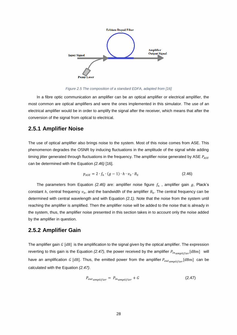
28
Figure 2.5 The composition of a standard EDFA, adapted from [16]
In a fibre optic communication an amplifier can be an optical amplifier or electrical amplifier, the
most common are optical amplifiers and were the ones implemented in this simulator. The use of an
electrical amplifier would be in order to amplify the signal after the receiver, which means that after the
conversion of the signal from optical to electrical.
2.5.1 Amplifier Noise
The use of optical amplifier also brings noise to the system. Most of this noise comes from ASE. This
phenomenon degrades the OSNR by inducing fluctuations in the amplitude of the signal while adding
timing jitter generated through fluctuations in the frequency. The amplifier noise generated by ASE 𝑃𝐴𝑆𝐸
can be determined with the Equation (2.46) [16].
𝑝𝐴𝑆𝐸 = 2 ∙ 𝑓𝑛 ∙ (𝑔 − 1) ∙ ℎ ∙ 𝑣0 ∙ 𝐵0 (2.46)
The parameters from Equation (2.46) are: amplifier noise figure 𝑓𝑛 , amplifier gain 𝑔, Plack’s
constant ℎ, central frequency 𝑣0, and the bandwidth of the amplifier 𝐵0. The central frequency can be
determined with central wavelength and with Equation (2.1). Note that the noise from the system until
reaching the amplifier is amplified. Then the amplifier noise will be added to the noise that is already in
the system, thus, the amplifier noise presented in this section takes in to account only the noise added
by the amplifier in question.
2.5.2 Amplifier Gain
The amplifier gain 𝐺 [dB] is the amplification to the signal given by the optical amplifier. The expression
reverting to this gain is the Equation (2.47), the power received by the amplifier 𝑃𝑖𝑛𝑎𝑚𝑝𝑙𝑖𝑓𝑖𝑒𝑟[dBm] will
have an amplification 𝐺 [dB]. Thus, the emitted power from the amplifier 𝑃𝑜𝑢𝑡𝑎𝑚𝑝𝑙𝑖𝑓𝑖𝑒𝑟[dBm] can be
calculated with the Equation (2.47).
𝑃𝑜𝑢𝑡𝑎𝑚𝑝𝑙𝑖𝑓𝑖𝑒𝑟 = 𝑃𝑖𝑛𝑎𝑚𝑝𝑙𝑖𝑓𝑖𝑒𝑟 + 𝐺 (2.47)

29
2.5.3 Amplifier Gain Saturation
The amplification of the optical signal showed some limitations. Firstly, the amplifier gain in Section 2.5.2
does not take into account that the gain is reduced if the power received by the amplifier is comparable
to the power saturation of the amplifier 𝑃𝑠𝑎𝑡𝑎𝑚𝑝𝑙𝑖𝑓𝑖𝑒𝑟 . Secondly, the optical amplifier cannot be amplified
the signal over the saturation power, this limitation will cause a phenomenon called Gain Saturation.
The amplifier gain will diminish as the signal power received 𝑃𝑖𝑛𝑎𝑚𝑝𝑙𝑖𝑓𝑖𝑒𝑟 by the amplifier converges to
the saturation power. The gain saturation can be observed in Figure 2.6 for a gain G0 at 30 [dB].
Figure 2.6 Saturated amplifier gain G as a function of the output power (normalised to the saturation power) for gain G0 at 30 [dB].
If the signal power received is equal or even more than the saturation power, the gain of the optical
amplifier will be zero. This saturation of the amplifier’s gain can be determined by the Equation (2.48)
[9], in which 𝑝𝑜𝑢𝑡𝑎𝑚𝑝𝑙𝑖𝑓𝑖𝑒𝑟 is the power emitted by the amplifier in Wats, 𝑔0 stands for the amplifier gain
and 𝑔 is for the true amplifier gain or saturated gain.
𝑔 = 𝑔0𝑒𝑥𝑝 (−𝑔 − 1
𝑔
𝑝𝑜𝑢𝑡𝑎𝑚𝑝𝑙𝑖𝑓𝑖𝑒𝑟
𝑝𝑠𝑎𝑡𝑎𝑚𝑝𝑙𝑖𝑓𝑖𝑒𝑟) (2.48)
Note that in the Equation (2.48) the parameters are in lower case since they are not in decibels.
Usually, the gain of the amplifier is presented in [dB], in order to convert it from [W] to [dB] the Equation
(2.49) is used.
𝐺 = 10 ∙ 𝑙og10 (𝑔) (2.49)

30
2.6 Optical Filter
The use of many channels is possible with WDM and with an optical transmitter with the capabilities to
emit more than one channel. The optical filter is used to separate and analyse each channel in specified
frequency, since every channel has a different wavelength, rejecting other frequencies. The relation
between wavelength 𝜆 and frequency 𝑣 is given by the Equation (2.1), where 𝑐 is the speed of light in
vacuum. The optical filter is also used to filter the signal in order to provide less noise, per example by
using the preamplification technic, further discussed in Section 2.4.2. The optical filter is able to filter
some of the noise caused by the preamplification if the bandwidth of the optical filter ∆𝑣𝑜𝑝𝑡 is lower than
the bandwidth of the receiver. The main objective of using an optical filter in this situation is providing
less noise reaching a better ONSR at the entrance of the optical receiver. The optical receiver
parameters that this simulator takes into account is the bandwidth of the filter and the sum of the filter’s
transmissivity. The sum of the transmissivity of the filter is the amount of power that is detected by a
specific channel from the neighbouring channels.
2.6.1 Crosstalk
When separating the channels, the optical filter can detect some of the power emitted by the adjacent
channels if the channel spacing is not big enough. With this phenomenon, the optical filter will add to
the signal noise that is referred to as out-of-band crosstalk. Note that crosstalk only happens if the
transmitted signal is using WDM, more than one channel since the crosstalk is a phenomenon where
channels interfere with the detection or transmission of other channels.
Out-of-band
Optical filters often leak a fraction of the signal power from adjacent channels that interfere with the
detection process. This type of crosstalk is called out-of-band or heterowavelength and it can be
observed in Figure 2.7. In Figure 2.7 it can be observed that the filter bandwidth ends up detecting some
of the adjacent channels power, if the difference between the channel’s frequency is not big enough,
this can be augmented by applying a bigger channel spacing. By detecting adjacent channels power it
ultimately adds a boost to the signal power with more power than the channel originally had. This type
of crosstalk can ultimately be avoided if the channels spacing is big enough.

31
Figure 2.7 Transmissivity of an optical filter with a 40-GHz bandwidth shown detecting other channels on the spectra of three 10-Gb/s channels separated by 50 GHz
So, in order to remove this additional power generated by crosstalk a power penalty needs to be
taken into account. This power penalty can be calculated with the Equation (2.50) [21], where 𝑅𝑛is the
responsivity of the nth channel, 𝑃𝑛is the power of the nth channel, 𝑇𝑚𝑛is the transmissivity between nth
and mth channels.
𝛿𝑋𝑜 = 10 ∙ 𝑙og10 (1 +∑ 𝑅𝑛𝑃𝑛𝑇𝑚𝑛𝑁𝑛≠𝑚
𝑅𝑛𝑃𝑚)
(2.50)
If the peak power is assumed to be the same for all channels and the responsivity is nearly the
same for all channels 𝑅𝑛 ≈ 𝑅𝑚 the Equation (2.50) can be approximated by the Equation (2.51), where
𝑋 is the parameter for the measure of the out-of-band crosstalk.
𝛿𝑋𝑜 ≈ 10 ∙ 𝑙og10 (1 + 𝑋) (2.51)
The parameter 𝑋 can be determined through the Equation (2.52). This parameter is the fraction of
the total power leaked into the detected power for a specific channel in a filter, which means that it is
the total out-of-band crosstalk measured by the system.
𝑋 =∑ 𝑇𝑚𝑛𝑁
𝑛≠𝑚
(2.52)
The transmissivity 𝑇𝑚𝑛 is the only parameter needed to calculate an approximate value to the power
penalty generated by the out-of-band crosstalk that can be determined combining Equations (2.51) and
(2.50). However typical values of 𝑋 such as 0.01 produce less than 0.1[𝑑𝐵] penalty.
In-band
In WDM components the filtering of the different wavelength for the different channels can be incomplete
because of partially overlapping transmission peaks. The penalty caused by the in-band can be
calculated with the Equation (2.53).

32
𝛿𝑋𝑖 = −10 ∙ 𝑙og10 (1 − 𝑄
2𝑟𝑋2) (2.53)
The Equation (2.53) can be determined by parameter 𝑄 from Equation (2.26) and parameter 𝑟𝑋
that can be determined with the Equation (2.54).
𝑟𝑋2 = 𝑋2(𝑁 − 1) (2.54)
Note that in the Equation (2.54) the parameter 𝑋2 is defined as the Equation (2.55) where 𝑃𝑛 is
the constant or all sources of in-band crosstalk and 𝑃0 is the input peak power.
𝑋2 =𝑃𝑛𝑃0
(2.55)
In practice 𝑃𝑛 ≪ 𝑃0 because the devices in the fibre such as the waveguide-grading router are built
to reduce this kind of crosstalk.
2.7 Power Penalty
In a fibre optical telecommunications system, there are many phenomena that degrade the signal that
reaches the receiver. In this section were included the power penalties that this simulator takes into
account. The power penalties that were included are the ones that have the biggest effect fibre optical
telecommunications system simulation. Note that the power penalty due to chromatic dispersion is
divided into two types dispersive pulse broadening and frequency chirping. Thus, the power penalty due
to chromatic dispersion is the sum of both power penalties.
2.7.1 Penalty due to Dispersive Pulse Broadening
To avoid the intermodal dispersion and the associated modal noise the use of single-mode fibres for
fibre optic communications is recommended since it nearly avoids this problem, but the group-velocity
dispersion limits the bit-rate distance product, by broadening optical pulses exceeding its allocated
value. The dispersion induced pulse broadening can also be calculated by a power penalty decreasing
the receiver sensitivity, that can be calculated with the Equation (2.56) [9].
𝛿𝑑 = −5 ∙ 𝑙og10 (1 − (4 ∙ 𝐵 ∙ 𝐿𝑇𝑜𝑡𝑎𝑙 ∙ 𝐷 ∙ 𝜎𝜆)
2) (2.56)
The penalty introduced by dispersive pulse broadening can be determined with the dispersion of
the fibre 𝐷, the total length of the fibre 𝐿𝑇𝑜𝑡𝑎𝑙, the bit-rate 𝐵 and the root mean square width of the source
spectrum 𝜎𝜆 in [m] from Equation (2.4).
33
2.7.2 Penalty due to the Frequency Chirping
A chirped optical pulse is an optical pulse with time-dependent phase shift, this means that the frequency
increases and decreases with time, thus its spectrum is considerably broadened resulting in degradation
of the system performance. The worst-case scenario for the penalty introduced by frequency chirping
can be determined with the Equation (2.57) [9], in which the value of the chirp parameter 𝐶 needs to be
given to the simulator.
𝛿𝑐 = 5 ∙ log [(1 + 8 ∙ 𝐶 ∙ 𝐵2 ∙ 𝐿𝑇𝑜𝑡𝑎𝑙
𝐷 ∙ 𝜆02
2𝜋 ∙ 𝑐)
2
+ (8 ∙ 𝐵2 ∙ 𝐿𝑇𝑜𝑡𝑎𝑙𝐷 ∙ 𝜆0
2
2𝜋 ∙ 𝑐)
2
] (2.57)
The parameters of the Equation (2.57) apart from the chirp parameter are the speed of light in
vacuum 𝑐, the dispersion of the fiber 𝐷, the wave-length 𝜆0, the bit-rate 𝐵 and the total length of the fibre
𝐿𝑇𝑜𝑡𝑎𝑙.
2.7.3 Penalty due to the Reflection Feedback
In a fibre optical telecommunications system, some light is reflected back where the refractive-index
discontinues, this discontinuation only happens in the splices, connectors and fibre ends. The reflected
light provokes an optical feedback degrading the performance light wave systems. The power penalty
caused by the optical feedback can be determined with the Equation (2.58) [9].
𝛿𝑟𝑒𝑓 = −10 ∙ 𝑙og10 (1 − 𝑄
2𝑟𝑒𝑓𝑓2) (2.58)
The Equation (2.58) can be determined by the parameters 𝑄 from Equation (2.26) and effective
intensity noise 𝑟𝑒𝑓𝑓 . The effective intensity noise can be determined with the Equation (2.59) [9] knowing
the relative intensity noise (RIN) and the receiver bandwidth ∆𝑓 .
𝑟𝑒𝑓𝑓
2 = 2 ∙ 𝑅𝐼𝑁 ∙ ∆𝑓 (2.59)
2.7.4 Penalty due to the Mode-Partition Noise
A semiconductor laser exhibits mode-partition noise (MPN) because of anticorrelation between pairs of
longitudinal modes, this anticorrelation makes the longitudinal modes fluctuate provoking large intensity
fluctuations in the individual modes. The existence of fibre dispersion is what makes MPN
unsynchronized different modes since they are transmitted at different speeds. Thus, the receiver
current exhibits additional fluctuations. The power penalty caused by MPN can be determined for a
required BER with the Equation (2.60) [9].
𝛿𝑚𝑝𝑛 = −5 ∙ 𝑙og10 (1 − 𝑄
2𝑟𝑚𝑝𝑛2) (2.60)
The Equation (2.60) can be determined parameters 𝑄 from Equation (2.26) and the relative noise
level of the receiver power 𝑟𝑚𝑝𝑛 that can be determined with Equation (2.61) [9].
34
𝑟𝑚𝑝𝑛 = (𝑘
√2) {1 − 𝑒𝑥𝑝[−(𝜋 ∙ 𝐵 ∙ 𝐿𝑇𝑜𝑡𝑎𝑙 ∙ 𝐷 ∙ 𝜎𝜆)
2]} (2.61)
The relative noise level of the receiver power can be determined with the bit-rate B, the dispersion
D, the total length of the fibre 𝐿𝑇𝑜𝑡𝑎𝑙 , the root mean square width of the source spectrum 𝜎𝜆 with Equation
(2.4) and the mode-partition coefficient k that ranges from [0;1].
2.8 Optical Signal to Noise Ratio
When planning a fibre optic telecommunication system, improving the received signal is always the
main concern. This improvement is important since it may help choose which components should be in
the system or which transmitted power or which gain. In order to evaluate the quality of the received
signal a parameter was designed, the OSNR. This parameter measures the ratio between the received
signal and its noise. Usually, this is the best way to analyse the performance of the fibre optic
telecommunication system. The OSNR can be determined in each component of the system, thus
evaluating its performance. The basic evaluation of the OSNR is in the Equation (2.62) [16], in which
𝑝𝑜𝑢𝑡 is the signal power and 𝑝𝑛 is the noise power.
𝑜𝑠𝑛𝑟 =𝑝𝑜𝑢𝑡𝑝𝑛
(2.62)
The Equation (2.62) shows how the 𝑜𝑠𝑛𝑟 is obtained in linear units and it is typically presented in
[𝑑𝐵], so Equation (2.62) can be used to convert it into [𝑑𝐵]. However, there can be another
representation of Equation (2.62), in order to obtain the result already in [𝑑𝐵], Equation (2.63).
𝑂𝑆𝑁𝑅 = 𝑃𝑜𝑢𝑡 − 𝑃𝑛 (2.63)
The OSNR is only valid if the signal to noise ratio is being determined for an optical signal. The
signal is converted to an electrical signal in the receiver, so within the receiver is not possible to
determine the OSNR. In a fibre optic telecommunication system, after the signal is converted to an
electrical signal, the parameter that can evaluate its quality is the SNR. Also, in order to have some
backup power, this means that the power reaching the receiver has to be higher than the necessary for
the system to run. This power can be allocated if some degradation of components is developed over
time that will cause new power penalties that the system did not consider. This allocation of power is
known as system margin 𝑀𝑠 that takes into account the needed power in order to achieve a reliable
communication and the received power leaving usually a margin of 6 [𝑑𝐵].
2.8.1 OSNR in the Transmitter
The simulator does not determine the transmitter OSNR, instead, it requires it to determine the noise
inserted on the system by the transmitter. The transmitter noise can be determined by Equation (2.64).

35
Please note that the OSNR of the transmitter is at the exit of this component since the signal is already
converted into an optical signal.
𝑃𝑛𝑡𝑟𝑎𝑛𝑠𝑚𝑖𝑡𝑡𝑒𝑟 = 𝑃𝑜𝑢𝑡𝑡𝑟𝑎𝑛𝑠𝑚𝑖𝑡𝑡𝑒𝑑 − 𝑂𝑆𝑁𝑅𝑡𝑟𝑎𝑛𝑠𝑚𝑖𝑡𝑡𝑒𝑟 (2.64)
Equation (2.64) can be determined if the transmitted power of the transmitter, 𝑃𝑜𝑢𝑡𝑡𝑟𝑎𝑛𝑠𝑚𝑖𝑡𝑡𝑒𝑑 , and
the optical signal to noise ration of the transmitter, 𝑂𝑆𝑁𝑅𝑡𝑟𝑎𝑛𝑠𝑚𝑖𝑡𝑡𝑒𝑟, are provided. The noise of the
transmitter will propagate throughout the system with the noise added by other components.
2.8.2 OSNR in the Optical Amplifier
The optical amplifier, mentioned in Section 2.5.1 also brings some noise into the system, the most
dominant being the noise generated by ASE. The noise power 𝑝𝑛 at the amplifier can be determined
using Equation (2.65) [16]. The parameter 𝑝𝑛𝑠 is the noise that is propagated in the system until that
point, including all the noise introduced by the previous amplifiers and by the optical transmitter.
𝑝𝑛 = 𝑝𝐴𝑆𝐸 + 𝑝𝑛𝑠 (2.65)
The noise from the system 𝑝𝑛𝑠 will be attenuated by the fibre. However, in the amplifier the noise
of the system will be amplified. Since the signal power is being amplified, the noise that is already in
the system will be amplified too. Thus, the noise system that is inserted in Equation (2.65) is determined
by Equation (2.66).
𝑃𝑛𝑠 = 𝑃𝑛𝑟𝑒𝑐𝑒𝑖𝑣𝑒𝑑 + 𝐺 (2.66)
Also, as it was mentioned in Section 2.5.2, the optical signal after the amplifier is given by the
Equation (2.47), so in the optical signal after the amplifier can also be represented by Equation (2.67)
[16], where 𝑝𝑖𝑛𝑎𝑚𝑝𝑙𝑖𝑓𝑖𝑒𝑟 is the power received by the amplifier and 𝑔 is the gain of the amplifier.
𝑝𝑜𝑢𝑡 = 𝑔 ∙ 𝑝𝑖𝑛𝑎𝑚𝑝𝑙𝑖𝑓𝑖𝑒𝑟 (2.67)
By combining Equation (2.62), Equation (2.65) and Equation (2.67), the OSNR at the end of the
optical amplifier can be determined by Equation (2.68):
𝑜𝑠𝑛𝑟𝑎 =𝑔 ∙ 𝑝𝑖𝑛𝑎𝑚𝑝𝑙𝑖𝑓𝑖𝑒𝑟
𝑝𝐴𝑆𝐸 + 𝑝𝑛𝑠 (2.68)
2.8.3 OSNR at the Optical Receiver
The OSNR can be determined at the entrance of the optical receiver, before is converted into an
electrical signal. The noise power that reaches the optical receiver is the sum of all the noise of the
system. This parameter does not differ between APD or PIN receivers, since the gain and noise insertion
from these receivers only affect the electrical signal. So, the noise power 𝑝𝑛 at the entrance of the

36
optical receiver can be determined by Equation (2.69) [16], where 𝑝𝑛𝑠 is the sum of all the noise of the
system until the signal reaches the receiver.
𝑝𝑛 = 𝑝𝑛𝑠 (2.69)
The 𝑝𝑜𝑢𝑡 is the received power by the optical receiver 𝑝𝑜𝑢𝑡 = 𝑝𝑖𝑛𝑟𝑒𝑐𝑒𝑖𝑣𝑒𝑟. By combining Equation
(2.62), Equation (2.69) and the received power, the OSNR at the end of the optical amplifier can be
determined with Equation (2.70)(2.68) .
𝑜𝑠𝑛𝑟𝑟 =𝑝𝑖𝑛𝑟𝑒𝑐𝑒𝑖𝑣𝑒𝑟𝑝𝑛𝑠
(2.70)
The OSNR Equation (2.70) is normally presented in [dB], so if Equation (2.63) is taken into account,
the OSNR at the end of the amplifier can be determined directly in [dB] with Equation (2.71).
𝑂𝑆𝑁𝑅𝑟 = 𝑃𝑖𝑛𝑟𝑒𝑐𝑒𝑖𝑣𝑒𝑟 − 𝑃𝑛𝑠 (2.71)
2.8.4 BER at the Optical Receiver
After the OSNR at the entrance of the receiver the BER can be determined. The required BER and the
BER determined at the entrance of the receiver are not the same thing. The BER at the receiver is the
total bit error rate of the system. On the other hand, the BER that is required by the receiver is used to
determine the sensitivity of the receiver. The BER required by the receiver is determined by the user,
so if the user requires a minor BER the sensitivity will be higher. Further discussion on this issue in
Section 2.4.1.
Firstly, in order to determine the BER at the entrance of the receiver, the parameter Q must be
calculated using Equation (2.72). The parameters in this equation have already been explained in the
previous sections. The parameter 𝑜𝑠𝑛𝑟𝑟 is the optical signal to noise ratio at the receiver.
𝑄 =
𝑜𝑠𝑛𝑟𝑟 ∙ √∆𝑣𝑜𝑝𝑡∆𝑓
√2 ∙ 𝑜𝑠𝑛𝑟𝑟 + 1 + 1
(2.72)
If the parameter Q is obtained, the BER at the entrance of the receiver can be determined using
Equation (2.23), since the relation between the BER and parameter Q does not change from Section
2.4.1.
2.8.5 SNR at the Optical Receiver
The OSNR can only be calculated until the entrance of the receiver, because after that the signal is
converted from an optical signal to an electrical signal. The SNR is the signal to noise ratio of the
electrical signal that reaches the receiver, in a way the SNR of the system. The two types of receivers
will have a different SNR from each other, because the APD receiver has a gain added to the signal,

37
but an added noise power from that gain. However, this added noise power can ultimately improve the
SNR of the receiver.
In Section 2.4, the concept of APD and PIN receivers is explained. The formulas used to determine
the sensitivity of the receiver do not differ, but the values used for the gain and noise are different for
each receiver, because usually the PIN receiver does not have a gain 𝑀𝑝𝑖𝑛 = 1. Nonetheless, there is
the possibility that a PIN receiver can have a gain, so the equation to determine the SNR Equation (2.73)
is the same for both. The only parameters that are different are the gain 𝑀 and the excess noise factor,
𝐹𝐴.
𝑠𝑛𝑟𝑟 =
(𝑀𝑅𝑝𝑖𝑛)2
𝑝𝑛𝑠 + 2𝑞𝑀2𝐹𝐴(𝑅𝑝𝑖𝑛 + 𝐼𝑑)∆𝑓 + 4 (
𝑘𝐵𝑇𝑅𝐿) 𝑓𝑛∆𝑓
(2.73)
The parameters from Equation (2.73) are the elementary charge 𝑞 [𝐶], the gain 𝑀, the excess
noise factor 𝐹𝐴, the received power 𝑝𝑖𝑛, the dark current 𝐼𝑑, the noise figure 𝑓𝑛, the responsivity 𝑅, 𝑘𝐵
the room temperature 𝑇 = 290 𝐾, the Boltzmann constant 𝑘𝐵 [𝐽/𝐾], the resistor 𝑅𝐿 = 1𝑘𝛺 and the
bandwidth of the receiver ∆𝑓. The parameter 𝑝𝑛𝑠 is the noise power that is propagated in the system, so
the SNR of the receiver takes into account the noise power of the system and the noise of the receiver
as well. Thus, the SNR of the receiver is in fact the signal to noise ratio of the system.
2.8.6 System Margin
The system margin is the allocated power in order to prevent the system failure in case of the
appearance of some power penalties that may develop due to degradation of components or other
events. Usually, the system margin needs to be at least 6𝑑𝐵 [16], this means that the difference between
the received power and the required power to maintain the system, minus the power penalties generated
in the transmission should leave a margin of at least 6𝑑𝐵. The equation used to determine the systems
margin is Equation (2.74), where 𝑃𝑖𝑛𝑟𝑒𝑐𝑒𝑖𝑣𝑒𝑟 is the received power at the receiver, 𝛿𝑑 is the power penalty
due to pulse broadening, 𝛿𝑐 is the power penalty due to chromatic dispersion, 𝛿𝑚𝑝𝑛 is the power penalty
due to MPN, 𝛿𝑟𝑒𝑓 is the power penalty due to reflection feedback, 𝛿𝑋𝑖 and 𝛿𝑋𝑜 are the both power
penalties due to crosstalk.
𝑀𝑠 = 𝑃𝑖𝑛𝑟𝑒𝑐𝑒𝑖𝑣𝑒𝑟 − 𝑃�̅�𝑟𝑒𝑎𝑙 − 𝛿𝑑 − 𝛿𝑐 − 𝛿𝑚𝑝𝑛 − 𝛿𝑟𝑒𝑓 − 𝛿𝑋𝑖−𝛿𝑋𝑜
(2.74)
The last parameter in Equation (2.74) that was not referred before is 𝑃�̅�𝑟𝑒𝑎𝑙 this parameter is the real
receiver sensitivity, which means that the receiver sensitivity mentioned before in Section 2.4.3 can be
degraded. Thus, in order to determine the real receiver sensitivity, Equation (2.75) must be used. As it
was discussed in Section 2.4, the average receiver sensitivity differs between PIN and APD or even if it
has preamplification or not. However, in Equation (2.75) the formula does not change in any way, only
𝑃�̅� is used accordingly.
𝑃�̅�𝑟𝑒𝑎𝑙 = 𝑃�̅� − 𝛿𝑒𝑥 − 𝛿𝐼 − 𝛿𝑗 (2.75)

38

39
Chapter 3
3. Simulator
implementation
The implemented simulator is a Simulink library, and even though the installation of the simulator is
straightforward, an explanation of its installation was provided in this section. This section also provides
an explanation on how to use the simulator and on how to change and use each component to facilitate
their comprehension. The last parts of this subsection are used to verify the accuracy of the results that
were obtained using the simulator. These tests were a result comparison between the simulator that
was implemented and another simulator. Finally, a real-life project was implemented to test the
capacities of the simulator, and a theoretical analysis of the results was done in order to verify the
accuracy of the results. The simulator can be accessed in the following url:
https://drive.google.com/open?id=0B94fXxJbjhdtNmE4aEY0ZmJOeXc
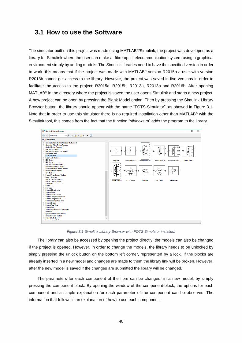
40
3.1 How to use the Software
The simulator built on this project was made using MATLAB®/Simulink, the project was developed as a
library for Simulink where the user can make a fibre optic telecommunication system using a graphical
environment simply by adding models. The Simulink libraries need to have the specified version in order
to work, this means that if the project was made with MATLAB® version R2015b a user with version
R2013b cannot get access to the library. However, the project was saved in five versions in order to
facilitate the access to the project: R2015a, R2015b, R2013a, R2013b and R2016b. After opening
MATLAB® in the directory where the project is saved the user opens Simulink and starts a new project.
A new project can be open by pressing the Blank Model option. Then by pressing the Simulink Library
Browser button, the library should appear with the name “FOTS Simulator”, as showed in Figure 3.1.
Note that in order to use this simulator there is no required installation other than MATLAB® with the
Simulink tool, this comes from the fact that the function “slblocks.m” adds the program to the library.
Figure 3.1 Simulink Library Browser with FOTS Simulator installed.
The library can also be accessed by opening the project directly, the models can also be changed
if the project is opened. However, in order to change the models, the library needs to be unlocked by
simply pressing the unlock button on the bottom left corner, represented by a lock. If the blocks are
already inserted in a new model and changes are made to them the library link will be broken. However,
after the new model is saved if the changes are submitted the library will be changed.
The parameters for each component of the fibre can be changed, in a new model, by simply
pressing the component block. By opening the window of the component block, the options for each
component and a simple explanation for each parameter of the component can be observed. The
information that follows is an explanation of how to use each component.

41
The data that the simulator returns is divided into three types: a text file, an excel document and
the Simulink outputs. These types of data are created by the receiver block, so they are explained with
more detail in Section 0
3.1.1 How to use the Optical Transmitter
The optical transmitter is the starting block for every fibre optic telecommunication systems simulation,
this block is the only one that can be connected directly to any block on the library. The parameter can
be changed by simply pressing on the transmitter block, representation in Figure 3.2. Also, the figure
allows identifying that every parameter already has a standard value. In the regards that the user does
not know the value of a specific parameter, it is recommended that the standard values remain the
same.
Figure 3.2 Transmitter block and window where its parameters can be edited
The main parameters of the transmitter are: the bit-rate, the signal power, the linewidth, the
wavelength and the central wavelength. In order to add more than one channel, the number of channels
must be inserted. Note that if the number of channels surpasses 10 channels, all the channels will have
the same linewidth and the same starting signal power. However, if the number of channels is between
the interval ]1, 10], the values for each signal power and respectively linewidth can be inserted in the
“Other Channels” tab. This constraint was implemented because the Simulink software requires a block
for each new parameter. Since infinite block cannot be added and would make the insertion of values
complicated, a decision was made to limit the number of custom channels that can be created with
different powers and linewidth. In addition, the value for the channel spacing must be changed in this
tab. The parameters tab has a collapsible panel that appears by pressing the “Other Parameters”, as it
can be observed in Figure 3.2. These parameters are associated with the power penalties and sensitivity
degradation, the last tab “More information” provides information about each parameter. Table 3.1
contains the standard parameters of the transmitter block.

42
Table 3.1 Default parameters of an optical transmitter
𝐵 [𝐺𝑏𝑝𝑠] 𝑃𝑒 [𝑑𝐵𝑚] ∆𝑣 [𝐺𝐻𝑧] 𝜆 [𝑛𝑚] 𝑂𝑆𝑁𝑅 [𝑑𝐵] ∆𝑣𝑐ℎ[𝐺𝐻𝑧] 𝑅𝑒𝑥 [𝑑𝐵] C 𝑅𝐼𝑁 [𝑑𝐵/𝐻𝑧 ]
𝐾 𝑡𝑗 [𝑛𝑠]
9,953 5 1 1550 40 50 10 0.5 −130 0.01 0.01
3.1.2 How to use the Optical Fibre
The optical fibre block can be inserted between the transmitter and the receiver, the use of this block is
the basic principle in each fibre optic telecommunications systems work. However, the user can connect
the transmitter directly to the receiver in order to test the losses of the system without the fibre. There
are two types of fibres built in this library as it was referred in Section 2.3. However, any type of fibre
should be possible to build with these blocks by simply modifying the parameters. The only difference
between the block using a SMF and NZDSF is that the standard parameter is specified following an
example of each type of fibre. The parameter of the fibre can be edited in the pop-up window opened
when pressing the block as the example Figure 3.3.
Figure 3.3 SMF fibre block and window where its parameters can be edited
The main parameters of the optical fibre can be edited in the main window, the fibre dispersion can
be presented in two ways, but if in the dispersion parameter tab is inserted a different value than 0 the
program will take it into account. There is also the attenuation of splices and connectors that are asked
in this block for means of simplification. The attenuation of the fibre can be inserted in three different
ways, the first one is by not adding any information about the fibre attenuation and the program will

43
assume that the values stay the same as the example G.655 or G.652, either if using a NZDSF fibre or
SMF fibre. The second way is to assume that the attenuation of the fibre does not change with the
frequency and it is given a constant value. The last one is giving specific values for specific intervals
defined by the user as can be observed in Figure 3.4.
Figure 3.4 NZDSF fibre block and window where its parameters can be edited
Although, there are only two types of fibres introduced in the program, they can always be changed.
This means that these types of fibres were the only ones that the standard values were already
implemented following an example for each fibre. However, the user can always customise each block
to replicate another type of fibre. The nonlinear effects throughout the fibre are verified in this block,
these effects take into account the sum of the power of every channel transmitted in the fibre. The
limitations of the nonlinear effects will only limit the threshold power or incident power in the fibre. Thus,
if any nonlinear effect surpasses the threshold power or incident power limitations this block will print a
warning message in the MATLAB® terminal and in a pop-up message (Figure 3.5).
Figure 3.5 Nonlinear effects warning from the fibre block
The standard values of the parameters for each type of fibre block are represented in Table 3.2.
Every attenuation parameter of each fibre is set as zero, this can be observed in Figure 3.4. Thus, these
parameters were not represented in Table 3.2.

44
Table 3.2 Default values for the fibre blocks
Fibre 𝐿𝑒𝑛𝑔𝑡ℎ [𝑘𝑚] 𝛽2 [𝑝𝑠2/𝑘𝑚] 𝛽3 [𝑝𝑠
3/𝑘𝑚] 𝜆𝑟 [𝑛𝑚] 𝑁𝑆 𝐴𝑆 [𝑑𝐵] 𝑁𝐶 𝐴𝐶 [𝑑𝐵] 𝐷𝑖𝑠
SMF 100 −24 0,1 1550 1 2 2 1 0
NZDSF 100 −2,8 0,08 1550 1 2 2 1 0
3.1.3 How to use the Optical Amplifier
The amplifier is used to amplify the signal’s power, moreover Section 2.5. This block can be inserted
any position between the optical transmitter and optical receiver, one example of its use is shown in
Figure 2.4. The amplifier parameters can be changed by pressing the amplifier block, which will open a
new window where the parameters can be inserted and with some information about each parameter,
an example of this is presented in Figure 3.6. An explanation for each parameter can be found in Section
2.5, the information found in that section is more detailed the information presented in the program.
Figure 3.6 Amplifier block and window where its parameters can be edited
The use of the technique preamplification presented in Section 2.4.2 will change the formula used
to calculate the average receiver sensitivity. So, in order for the program to calculate the value correctly
the last parameter on the pop-up window must be inserted “1”. If the parameter is “0” the simulator will
assume that there is no preamplification in the system. Table 3.3 contains the standard values that are
implemented in the amplifier block, these values can be altered by submitting new values and a simple
explanation of each one is presented in the block window.
Table 3.3 Standard values for the Amplifier block
𝐹𝑛 [𝑑𝐵] 𝑃𝑠 [𝑑𝐵𝑚] 𝐺 [𝑑𝐵] 𝐵0 [𝑛𝑚] 𝑃𝑟𝑒
3 30 30 0,3 0
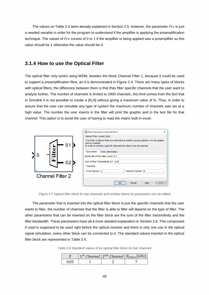
45
The values on Table 3.3 were already explained in Section 2.5, however, the parameter 𝑃𝑟𝑒 is just
a needed variable in order for the program to understand if the amplifier is applying the preamplification
technique. The values of 𝑃𝑟𝑒 consist of 0 or 1 if the amplifier is being applied was a preamplifier so this
value should be 1 otherwise the value should be 0.
3.1.4 How to use the Optical Filter
The optical filter only works using WDM, besides the block Channel Filter 1, because it could be used
to support a preamplification fibre, as it is demonstrated in Figure 2.4. There are many types of blocks
with optical filters, the difference between them is that they filter specific channels that the user want to
analyse further. The number of channels is limited to 2000 channels, this limit comes from the fact that
in Simulink it is not possible to create a [N,N] without giving a maximum value of N. Thus, in order to
assure that the user can simulate any type of system the maximum number of channels was set at a
high value. The number the user inserts in the filter will print the graphic and in the text file for that
channel. This option is to avoid the user of having to read the matrix built in excel.
Figure 3.7 Optical filter block for two channels and window where its parameters can be edited
The parameter that is inserted into the optical filter block is just the specific channels that the user
wants to filter, the number of channels that the filter is able to filter will depend on the type of filter. The
other parameters that can be inserted on the filter block are the sum of the filter transmitivity and the
filter bandwidth. These parameters have all a more detailed explanation in Section 2.6. This component
if used is supposed to be used right before the optical receiver and there is only one use in the optical
signal simulation, every other block can be connected to it. The standard values inserted in the optical
filter block are represented in Table 3.4.
Table 3.4 Standard values of an optical filter block for two channels
𝑋 1𝑠𝑡 𝐶ℎ𝑎𝑛𝑛𝑒𝑙 2𝑛𝑑 𝐶ℎ𝑎𝑛𝑛𝑒𝑙 𝐵𝑓𝑖𝑙𝑡𝑒𝑟[𝐺𝐻𝑧]
0,05 1 2 7

46
3.1.5 How to use the Optical Receiver
The optical receiver is the block that will receive the optical signal and convert it into an electrical signal.
This block is supposed to be the last block of the system in this simulator, so any other block can connect
to it. There are two types of receivers implemented in the simulator, PIN receiver and APD receiver
instead of providing both types of blocks there is only one. The parameters of the receiver block can be
modified in the block window, represented in Figure 3.8.
Figure 3.8 Receiver fibre block and window where its parameters can be edited
The decision of having both types of receivers was made in order to provide the user with a
comparison between both receivers by observing the difference between the SNR achieved and the
system margin. The comparison between them can be observed in many ways since the information
provided by the simulator has three types of sources. The information can be taken for the excel file
created by the program called “Data.xlsx”, this file contains the main matrix of the program, this matrix
contains all the main parameters that needed to be shared for each block. The size of this matrix can
go from [1 34] to [2000 200], the reason behind it is [1 34] is or the smallest systems possible with only
one channel and with a transmitter and receiver. The 34 is the number of parameters that are needed
to run the systems simulation, this number will rise with the number of components since each time an
amplifier is added two new parameters are added to the matrix. This will depend on the number of
channels since the maximum is 2000 but also on the number of amplifier blocks that can be added, the
maximum number of amplifiers is (200-34)/2 = 83. The decision for limiting the maximum size can seem
arbitrary but this comes from the fact that when using Simulink, a matrix can have a variable size.
However, the maximum size must be defined, which means that a maximum number of parameters
must be stated. Thus, the limitation of the matrix was set to very high values usually the number of
channels can go up to 300 and the number of amplifiers should not be higher than 20. Even with this
limitation the program can be adapted to receive more parameters but each block and subblock have
to be changed manually in the Explore option of Simulink option.
There is always another way to analyse the system by opening the “ChanelX.txt” file that
corresponds to the Xth channel. This file can be found in the folder “Values” and there is one file for each

47
channel so the user can open a specific channel and observe a simple overview of the signal
propagation through the channel. The objective of this source of data is to analyse a channel
independently from other channels, Figure 3.9 show an example. This example is from a standard fibre
optic telecommunications system consisting of two fibres one amplifier and obviously one transmitter
and one receiver.
Figure 3.9: Example of a source of data printed in a text file
Figure 3.9 can be analysed and easily obtain all the important data throughout the fibre such as
the OSNR of each parameter that adds noise, the attenuation of the fibre, the distortion, etc. Note that
these parameters can only be an easy way to observe the parameters that were inserted by the user
and correct mistakes if necessary. One of the last important details of the data provided by this file is
the gain of the amplifier since the amplifier can be saturated and the user does not notice it, so if the
user inserts a gain it does not mean that the amplifier will amplify the signal with that gain, moreover
Section 2.5.3.
The last kind of data source provided by the simulator are outputs of Simulink this consists of a
graphical analysis of the OSNR throughout the fibre either from the first channel if a channel is not
specified or from a specified channel using the filter block. The receiver will also provide a graphical
analysis of the signal OSNR by wavelength if more than one channel is provided so the user can observe
that each wavelength provides an optimal OSNR for the system, Figure 3.11 shows an example of such
graphs. There is also a graphical analysis of the systems margin by each wavelength with equal intent
to the previous one. The output sources also consist of important information being printed in the
MATLAB® message box from the parameter values presented in Figure 3.10. There can also be

48
warnings if the threshold power surpasses the limitations on which the nonlinear effects will have to be
taken into account, or simple warnings such as non-compatible values and so forward.
Figure 3.10 Message box return from the simulator
The receiver block also returns three graphical analysis of the system. The first one is represented
in Figure 3.11. This figure includes two types of graphics: the OSNR throughout the fibre and the power
throughout the fibre.
Figure 3.11 Graphical analysis of the OSNR and power throughout the fibre
The second type of graphical analysis that is presented in this simulator can only be represented if
more than one channel is used. The reason behind it is that Figure 3.12 is a comparison between the
OSNR of each channel, where the graphic shows a similar variation with the different attenuations
parameters of the fibre through wavelength.

49
Figure 3.12 OSNR per wavelength
The last type of graphical analysis is Figure 3.13, which contains a graphical analysis of the systems
margin for every channel. The graphical representation shows the minimum required systems margin
represented in red. By analysing Figure 3.13, it can be taken into consideration that the wavelengths
from 1520 [𝑛𝑚] to 1540 [𝑛𝑚] are the only ones that comply with the minimum systems margin, for this
example.
Figure 3.13 Systems Margin for PIN and APD receivers
The receiver block also displays a warning error if the power penalty due to chromatic dispersion
surpasses the maximum value of 2 [𝑑𝐵] [21]. Figure 3.14 represents the warning message that is
displayed. A similar warning is presented if the overload power of the receiver is surpassed.
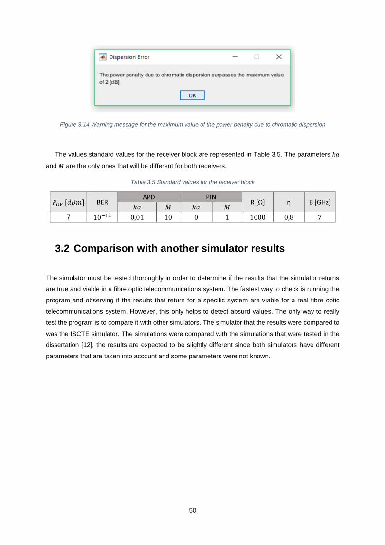
50
Figure 3.14 Warning message for the maximum value of the power penalty due to chromatic dispersion
The values standard values for the receiver block are represented in Table 3.5. The parameters 𝑘𝑎
and 𝑀 are the only ones that will be different for both receivers.
Table 3.5 Standard values for the receiver block
𝑃𝑂𝑉 [𝑑𝐵𝑚] BER APD PIN
R [Ω] η B [GHz] 𝑘𝑎 𝑀 𝑘𝑎 𝑀
7 10−12 0,01 10 0 1 1000 0,8 7
3.2 Comparison with another simulator results
The simulator must be tested thoroughly in order to determine if the results that the simulator returns
are true and viable in a fibre optic telecommunications system. The fastest way to check is running the
program and observing if the results that return for a specific system are viable for a real fibre optic
telecommunications system. However, this only helps to detect absurd values. The only way to really
test the program is to compare it with other simulators. The simulator that the results were compared to
was the ISCTE simulator. The simulations were compared with the simulations that were tested in the
dissertation [12], the results are expected to be slightly different since both simulators have different
parameters that are taken into account and some parameters were not known.

51
3.2.1 Case Study
The case study is presented in chapter 5 of the dissertation, which consists of a connection between
Lisbon and Porto with a distance of about 280 kilometres. The system involved two amplifiers and four
fibres with a length of 80 kilometres. The last section was shorter since the distance is only 280, so the
last one was assumed to have 40 kilometres. The representation of the systems built using the simulator
is represented in Figure 3.15.
Figure 3.15 The system that was built using the simulator
The input values were presented in snapshots of the simulator. However, there are some
parameters that this program takes into account that were not presented. This problem was resolved by
keeping the default values of the components or in some cases adapting the values in order to achieve
a similar representation with the project presented. The parameters inserted in the transmitter block are
represented in Figure 3.16.
Figure 3.16 The transmitter block parameter for the case study comparison
The last four parameters and the linewidth were not presented in the dissertation, so the parameter
values stayed the same as the standard value. However, the chirp parameter was set to zero because
it is referred to the project that the system is using external modulation. Thus, as it was discussed in
Section 2.2 the use of external modulation is commonly used in order to remove the chirping of the
frequency to improve the system performance.

52
The optical fibre blocks are basically the same although the last one has smaller dimensions as it
was mentioned before. The parameters can be observed in Figure 3.17. The only parameter of the fibre
that cannot be observed in the figure is the attenuation of the fibre, which was not presented in the
project presentation. However, it is said that the system uses SMF-28 fibre so typical values were
inserted in order to achieve the same attenuation.
Figure 3.17 The fibre block parameter for the case study comparison
Note that one of the major differences between both projects is that in this project, DCF fibres were
not implemented. These fibres are used to compensate dispersion in the fibre. Since in the other project
there are more 13.6 kilometres of DCF it is normal that the attenuation in each fibre is greater than the
one that will be obtained by this simulator. The loss of the fibre, in this project, is adapted in order to
achieve the same attenuation values of that project. This decision was made based on the fact that the
attenuation in the fibre is a parameter that does not need much testing. The optical fibre can be seen as
a black box that achieves a specific attenuation at the end of the fibre, as this simulator is already
describing.
The amplifier parameters are all presented in the dissertation. However, the noise figure of the
amplifier is not. Therefore, in order to determine the noise figure of the amplifiers the simulation was
tested with several typical values that the noise figure can have. The parameter value that was
compared to determine the noise figure was the ASE noise power since the other parameters were
presented in the project, obtaining a value of 𝐹𝑛 = 6 𝑑𝐵. The parameters inserted in the amplifier block
are presented in Figure 3.18. The gain of the amplifiers is equal to the losses in the fibre and both
amplifiers have exactly the same parameters.

53
Figure 3.18 The amplifier block parameter for the case study comparison
The last block used was the receiver block, the only information that was given about this block
was the required BER and that a PIN receiver is used. Since in this program the receiver block takes
into account a PIN receiver and an APD receiver at the same time, there is no necessity to change
anything. The parameters inserted in the receiver block are presented in Figure 3.19.
Figure 3.19 The receiver block parameter for the case study comparison
The results present in the simulator are compared and discussed in order to understand their
differences. These parameters are presented in Table 3.6, where number 1 represents the other
simulator and number 2 represents this simulator. The first parameter is the ASE noise power obtained
in each amplifier. This noise power is the same in both amplifiers because they have the same
parameters. These parameters are really similar and it is normal since the noise power inserted in order
to run this simulation was based on a comparison between the ASE noise power of both simulators. The
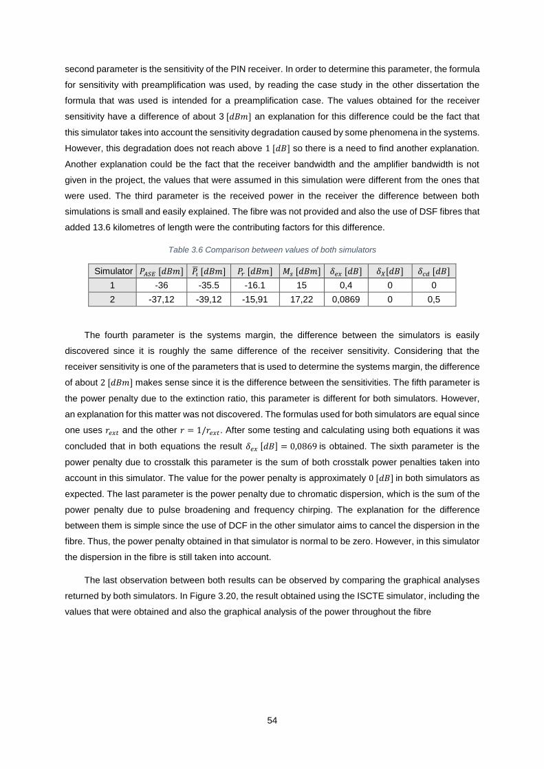
54
second parameter is the sensitivity of the PIN receiver. In order to determine this parameter, the formula
for sensitivity with preamplification was used, by reading the case study in the other dissertation the
formula that was used is intended for a preamplification case. The values obtained for the receiver
sensitivity have a difference of about 3 [𝑑𝐵𝑚] an explanation for this difference could be the fact that
this simulator takes into account the sensitivity degradation caused by some phenomena in the systems.
However, this degradation does not reach above 1 [𝑑𝐵] so there is a need to find another explanation.
Another explanation could be the fact that the receiver bandwidth and the amplifier bandwidth is not
given in the project, the values that were assumed in this simulation were different from the ones that
were used. The third parameter is the received power in the receiver the difference between both
simulations is small and easily explained. The fibre was not provided and also the use of DSF fibres that
added 13.6 kilometres of length were the contributing factors for this difference.
Table 3.6 Comparison between values of both simulators
Simulator 𝑃𝐴𝑆𝐸 [𝑑𝐵𝑚] 𝑃�̅� [𝑑𝐵𝑚] 𝑃𝑟 [𝑑𝐵𝑚] 𝑀𝑠 [𝑑𝐵𝑚] 𝛿𝑒𝑥 [𝑑𝐵] 𝛿𝑋[𝑑𝐵] 𝛿𝑐𝑑 [𝑑𝐵]
1 -36 -35.5 -16.1 15 0,4 0 0
2 -37,12 -39,12 -15,91 17,22 0,0869 0 0,5
The fourth parameter is the systems margin, the difference between the simulators is easily
discovered since it is roughly the same difference of the receiver sensitivity. Considering that the
receiver sensitivity is one of the parameters that is used to determine the systems margin, the difference
of about 2 [𝑑𝐵𝑚] makes sense since it is the difference between the sensitivities. The fifth parameter is
the power penalty due to the extinction ratio, this parameter is different for both simulators. However,
an explanation for this matter was not discovered. The formulas used for both simulators are equal since
one uses 𝑟𝑒𝑥𝑡 and the other 𝑟 = 1/𝑟𝑒𝑥𝑡. After some testing and calculating using both equations it was
concluded that in both equations the result 𝛿𝑒𝑥 [𝑑𝐵] = 0,0869 is obtained. The sixth parameter is the
power penalty due to crosstalk this parameter is the sum of both crosstalk power penalties taken into
account in this simulator. The value for the power penalty is approximately 0 [𝑑𝐵] in both simulators as
expected. The last parameter is the power penalty due to chromatic dispersion, which is the sum of the
power penalty due to pulse broadening and frequency chirping. The explanation for the difference
between them is simple since the use of DCF in the other simulator aims to cancel the dispersion in the
fibre. Thus, the power penalty obtained in that simulator is normal to be zero. However, in this simulator
the dispersion in the fibre is still taken into account.
The last observation between both results can be observed by comparing the graphical analyses
returned by both simulators. In Figure 3.20, the result obtained using the ISCTE simulator, including the
values that were obtained and also the graphical analysis of the power throughout the fibre

55
Figure 3.20 The graphical analysis of the cases study presented by the ISCTE simulator [12]
Figure 3.20 can be compared with Figure 3.21, both show a similar decline in the system’s power.
Even though the systems have different received powers, they are simulating the same system. The
comparison between both figures is only between the graphic from Figure 3.20 and the last graph of
Figure 3.21. The first graphic is the OSNR throughout the fibre and it cannot be compared since the
ISCTE simulator does not provide one.
Figure 3.21 The output of the case study received by the simulator built in this project

56
3.3 Testing the simulator in a real-life project
3.3.1 Presenting the Project
The objective of the simulator is to run real life projects and run the exact system in a computerised
environment. So, in order to test the capacity of this simulator a real-life project should be tested. The
project that was chosen was the fibre optic telecommunications system that was made by Fundação
para a Computação Cientifíca Nacional (FCCN) is a part of the Fundação para a Ciência e a Tecnologia
(FCT). The main mission of this foundation is to plan and manage the infrastructure of digital research
covering Portugal. Their services are available in education and research institutions, Instituto Superior
Técnico (IST) has the available data from this project.
The project consists of a fibre optic telecommunications system connecting all major universities
from Braga to Lisbon, a demonstration of the project is represented in Figure 3.22. However, for means
of simplification and since this program simulates only a point to point connect, the local networks and
connection to the universities were not taken into account only the connection from station Braga until
station Oriente in Lisbon.
Figure 3.22 The FCCN network from the provided data
The information provided for each connection consists of the length of the fibre, the attenuation per
kilometre for some wavelength, the dispersion of the fibre and the insertion losses of the fibre which can
be observed in Table 3.7. Note that in this table the values of the fibre were obtained to multiple
experiments and this information was provided by IST. The values for the attenuation and dispersion
from Table 3.7 are only for the wavelength 1550 [𝑛𝑚]. The stations between Braga and Oriente were
considered to be amplifiers that amplify the signal with a gain equal to the attenuation of the fibre.

57
Table 3.7 Values obtained from the project
Sections Length
[km] Insertion
losses [dB] Dispersion [ps/km/nm]
Attenuation [dB/km]
Sta. Braga to Sta. Campanhã
56,9 11,5 15,33 0,217
Sta. Campanhã to Sta. Aveiro
67,3 14 16,34 0,221
Sta. Aveiro to Sta. Coimbra 58,1 12 16,55 0,245
Sta. Coimbra to Sta. Vermoil 58,5 11,5 16,75 0,265
Sta. Vermoil to Sta. Entroncamento
57,7 11,4 16,23 0,265
Sta. Entroncamento to Sta. Setil
53,3 11 16,23 0,258
Sta. Setil to Sta. Oriente 52,4 11 16,38 0,203
The data from Table 3.7 has the only parameters that are already defined by the network. The rest
of the parameters of the fibre optic telecommunications system were not provided. Thus, the decisions
on what parameters to use were adapted to the project, such as the gain of the amplifiers since they are
usually equal to the attenuation of the fibre. Another information that was given about the project is that
the type of fibre used in the system was a SMF fibre, the rest of the decisions are presented in the next
section. The connection as a length of approximately 400 kilometres and Figure 3.23 has a
representation of the network in a map.
Figure 3.23 Map of the project

58
3.3.2 Project Simulation
The first thing to introduce in order to build this system is to open a new window, add a transmitter block
and edit the parameters for the transmitter. The project was divided into two implementations: in the first
one a transmitter with internal modulation was used and in the second one an external modulation was
used. The representation of the system in the simulator is presented in Figure 3.24.
Figure 3.24 Representation of the FCCN project in the simulator
The considerations for this system were every amplifier gain is equal to the loss of the fibre before
it, there is a use of preamplification on the last amplifier before the receiver and the parameters of the
transmitter are presented in Table 3.8. The only parameter that is missing in that table is the number of
channels that is 32 channels.
Table 3.8 Transmitter parameters for FCCN project simulation
𝐵 [𝐺𝑏𝑝𝑠] 𝑃𝑒 [𝑑𝐵𝑚] ∆𝑣 [𝐺𝐻𝑧] 𝜆 [𝑛𝑚] 𝑂𝑆𝑁𝑅 [𝑑𝐵] ∆𝑣𝑐ℎ[𝐺𝐻𝑧] 𝑅𝑒𝑥 [𝑑𝐵] C 𝑅𝐼𝑁 [𝑑𝐵/𝐻𝑧 ]
𝐾 𝑡𝑗 [𝑛𝑠]
2,5 0 1 1550 40 50 10 0,5 −130 0,01 0,01
The first implementation of the project used an internal modulation, which means that the chirp
parameter needed to be taken into account. The chirp parameter was set as 0.5, a standard value for
this parameter. For the external modulation, the only difference in the parameters was that the chirp
parameter was set as 0. Figure 3.25 shows the values that were inserted in each parameter. Since the
number of channels surpasses 10 channels, the transmitted power and the linewidth of the 32 channels
is the same as the one that was implemented for the first channel.

59
Figure 3.25 Transmitter block parameters for the FCCN simulation project.
The wavelength for the first channel is 1550 [𝑛𝑚], and since the channel spacing is set as ∆𝑣𝑐ℎ =
50 [𝐺𝐻𝑧], the wavelength of each channel is compressed in the interval [1537,68 ; 1550,00] [𝑛𝑚]. The
𝑂𝑆𝑁𝑅 at the exit of the transmitter was set as 40 [𝑑𝐵] because it is the standard value for the 𝑂𝑆𝑁𝑅 of
the transmitter. The bit-rate was set as 2.5 [𝐺𝑏𝑝𝑠] and the rest of the values kept the standard values
(Figure 3.25). The system was also tested with a bit-rate was set as 10 [𝐺𝑏𝑝𝑠]. However, the dispersion
penalty in the system surpassed the maximum value that is set for this parameter and the bit-rate was
changed to 2.5 [𝐺𝑏𝑝𝑠] in order to meet the requirements for the maximum power penalty due to
dispersion.
The fibre links that connect each station were SMF-28 fibres. Their parameters were different
according to the information provided for each connection (Table 3.7). The insertion loss of each fibre
was taken into account as the loss from the splices and connectors. The values from Table 3.7 were
inserted in the fibre block represented in Figure 3.26.
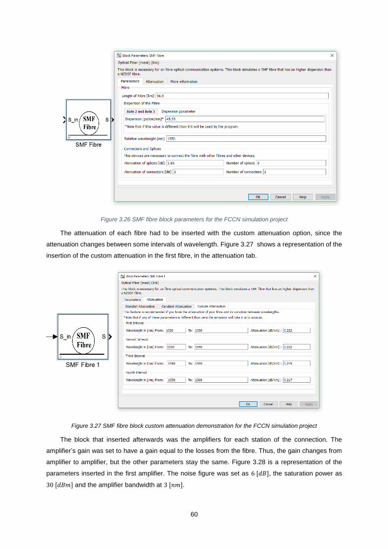
60
Figure 3.26 SMF fibre block parameters for the FCCN simulation project
The attenuation of each fibre had to be inserted with the custom attenuation option, since the
attenuation changes between some intervals of wavelength. Figure 3.27 shows a representation of the
insertion of the custom attenuation in the first fibre, in the attenuation tab.
Figure 3.27 SMF fibre block custom attenuation demonstration for the FCCN simulation project
The block that inserted afterwards was the amplifiers for each station of the connection. The
amplifier’s gain was set to have a gain equal to the losses from the fibre. Thus, the gain changes from
amplifier to amplifier, but the other parameters stay the same. Figure 3.28 is a representation of the
parameters inserted in the first amplifier. The noise figure was set as 6 [𝑑𝐵], the saturation power as
30 [𝑑𝐵𝑚] and the amplifier bandwidth at 3 [𝑛𝑚].

61
Figure 3.28 Amplifier block parameters for the FCCN simulation project
The last amplifier before the receiver is a preamplifier, so the last value of the amplifier block was
set as “1”. The last block inserted in the system was the receiver. The values from this block were not
changed from the standard values as it can be observed in Figure 3.29.
Figure 3.29 Receiver block parameters for the FCCN simulation project
3.3.2.1 Project with Internal Modulation
The first test of the FCCN project simulation used an internal modulation. As it was mentioned before,
the difference of using internal and external modulation with this simulator is that the chirp parameter
was set as 0.5. The values obtained for the transmitter are represented in Figure 3.30, these values do
not add any other information about the transmitter, beside the transmitter noise. The value for the
transmitter noise is determined if the values of the OSNR and transmitted power are known.

62
Figure 3.30 Transmitter message box in FCCN system
The values obtained in each amplifier and provided by the respective message box are represented
in Table 3.9. The parameters mentioned are: the received power 𝑃𝑟, the received noise 𝑃𝑛𝑟, the gain 𝐺,
the transmitted power 𝑃𝑡, the transmitted noise 𝑃𝑛𝑡, the ASE noise power or the noise of the amplifier
𝑃𝐴𝑆𝐸 and the 𝑂𝑆𝑁𝑅 at the end of the amplifier.
Table 3.9 Amplifier values provided by the amplifier message box in FCCN system
𝐴𝑚𝑝𝑙𝑖𝑓𝑖𝑒𝑟𝑠 𝑃𝑟 [𝑑𝐵𝑚] 𝑃𝑛𝑟 [𝑑𝐵𝑚] 𝐺 [ 𝑑𝐵] 𝑃𝑡 [𝑑𝐵𝑚] 𝑃𝑛𝑡 [𝑑𝐵𝑚] 𝑃𝐴𝑆𝐸 [𝑑𝐵𝑚] 𝑂𝑆𝑁𝑅 [𝑑𝐵]
1 −23,96 −63,96 25 1,04 −19,15 −36,18 20,19
2 −27,97 −48,16 30 2,03 −12,72 −31,17 14,75
3 −24,32 −39,07 28 3,68 −9,90 −33,17 13,59
4 −27,38 −40,97 30 2,62 −12,72 −31,17 11,89
5 −24,13 −36,02 28 3,87 −7,40 −33,17 11,28
6 −20,83 −32,10 22 1,17 −9,84 −39,14 11,02
7 −23,96 −63,96 25 1,04 −19,15 −36,18 20,19
The values of the transmitted power of the amplifier are the only values that are consistent. This
comes from the fact that the amplifier gain changes in order to keep the transmitted power of the
amplifiers similar to the transmitted power of the transmitter, 0 [𝑑𝐵𝑚]. The objective of doing this is the
same as keeping the amplifier’s gain equal to the attenuation in the fibre. This power is not exactly equal
to the loss of the receiver, this happened because after the simulation, it was discovered that if the
power was kept at 0 [𝑑𝐵𝑚], the system’s margin would be lower than 6 [𝑑𝐵]. The correct approach
would be to add a preamplifier, but the difference was approximately 3 [𝑑𝐵]. Thus, it did not make sense
to add an amplifier with a such lower gain and using a preamplifier would change the formula for the
sensitivity, and ultimately the system would end up having a system margin approximately to 30 [𝑑𝐵],
which would be too much backup power. The final solution that was implemented was to add some
power to the amplifiers that result in the power at the end of the amplifiers being slightly over 0 [𝑑𝐵𝑚].

63
The received power and received attenuation differ from each amplifier, since these values are
attenuated in the fibres and each fibre has different length and attenuation. However, the values of the
noise power received seem to be increasing, because the noise was accumulated throughout the
systems. Even though the noise power is attenuated in the fibre, the noise is amplified in the amplifier,
equal to the losses in the fibre and also ads the noise power of the new amplifier. The 𝑂𝑆𝑁𝑅 keeps
decreasing due to reasons presented before. The transmitted power is kept similar throughout the fibre
and the noise power keeps increasing. However, it can be observed in Figure 3.31 and the values in
Table 3.9 that the 𝑂𝑆𝑁𝑅 keeps decreasing at slower pace, even though the noise figure for each
amplifier is still 6 [𝑑𝐵]. The reason for this phenomenon is the fact that the noise power in the fourth
amplifier is already at a value, in which the added noise power afterwards is not that different from the
existing noise in the system. Also, Figure 3.31 shows a graphic of the power in the fibre. The last two
power values are the same, since between the preamplifier and the receiver there is no source of power
loss.
Figure 3.31 Graphical analysis provided by the simulator of the OSNR and power thought out the fibre
The loss of power in the last section of the fibre is due to the fact that no preamplifier was used.
Thus, the last attenuation caused by the last section was not amplified until the signal reaches the
receiver. The final results from the simulation are obtained by the receiver (Figure 3.32). There are two
types of values that are obtained, because the receiver block works as a PIN receiver and as an APD
receiver at the same time.

64
Figure 3.32 Receiver message box in FCCN system with internal modulation
Through comparing the receiver sensitivity for each type of receiver, it can be concluded that for
this case the APD receiver has the bigger system margin. This conclusion is possible since a greater
sensitivity will result in a bigger system margin, and this assumption can be observed in Figure 3.32.
The value for the 𝑂𝑆𝑁𝑅 is the same for both types of receivers, since is the signal to noise ratio of the
optical signal before reaching the receiver. The 𝑆𝑁𝑅 at the receiver will be lower, because it takes into
account the inserted noise from the receiver and all the other noise that reaches the receiver.
The non-linear effects taken into account did not report any detection. Thus, it is not necessary to
change the system power in order to comply with the non-effects requirements. The OSNR changes per
wavelength, this phenomenon can be observed in Figure 3.33. The changes in the OSNR presented in
the graphic of Figure 3.33 have an abrupt variation, this phenomenon happens in this project because
the information of the attenuation in the fibre changes abruptly and not gradually, these values can be
observed in Figure 3.28. The received power also does not surpass the overload power. The received
power is lower than 7 [𝑑𝐵𝑚] and the warning message if this value was surpassed was not showed. In
addition, the maximum value for the power penalty due to chromatic dispersion was not surpassed since
the value for this power penalty was around 0,11 [𝑑𝐵] and the maximum value is 2 [𝑑𝐵].
Figure 3.33 Graphical analyses of the OSNR per wavelength in the FCCN system
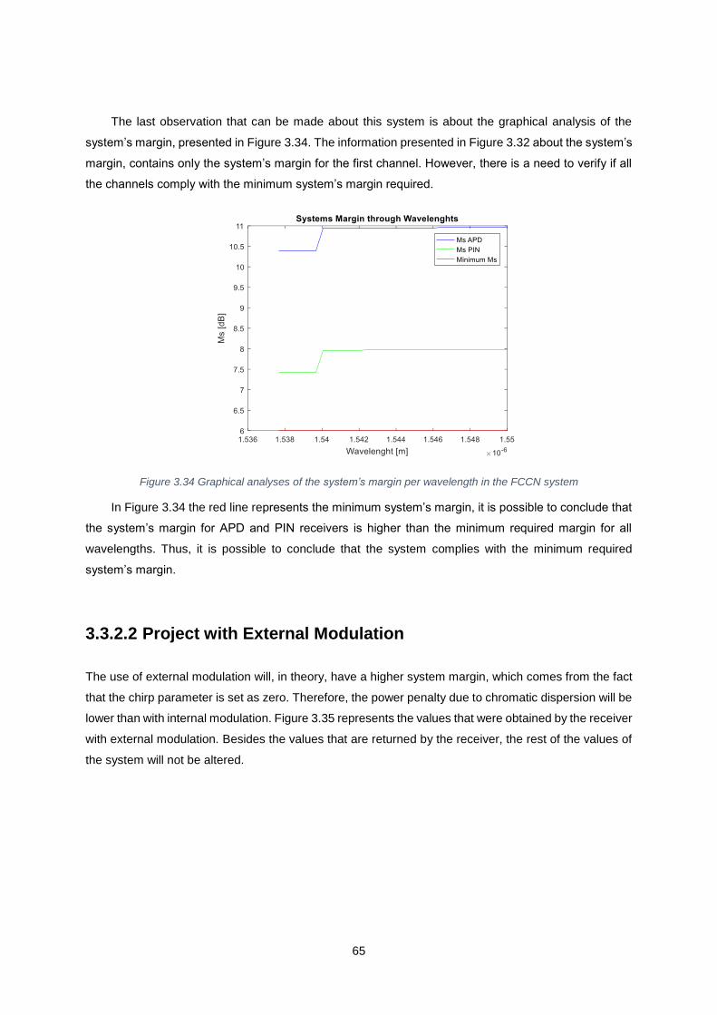
65
The last observation that can be made about this system is about the graphical analysis of the
system’s margin, presented in Figure 3.34. The information presented in Figure 3.32 about the system’s
margin, contains only the system’s margin for the first channel. However, there is a need to verify if all
the channels comply with the minimum system’s margin required.
Figure 3.34 Graphical analyses of the system’s margin per wavelength in the FCCN system
In Figure 3.34 the red line represents the minimum system’s margin, it is possible to conclude that
the system’s margin for APD and PIN receivers is higher than the minimum required margin for all
wavelengths. Thus, it is possible to conclude that the system complies with the minimum required
system’s margin.
3.3.2.2 Project with External Modulation
The use of external modulation will, in theory, have a higher system margin, which comes from the fact
that the chirp parameter is set as zero. Therefore, the power penalty due to chromatic dispersion will be
lower than with internal modulation. Figure 3.35 represents the values that were obtained by the receiver
with external modulation. Besides the values that are returned by the receiver, the rest of the values of
the system will not be altered.

66
Figure 3.35 Receiver message box in FCCN system with external modulation
The system’s margin, observed in Figure 3.32 and Figure 3.35, is higher with external modulation,
following the theoretical analysis that was set beforehand. It can be concluded that the use of external
modulation can be beneficial to the system, in this case, the system margin is significantly higher than
the minimum value for this parameter, 𝑀𝑠 > 6[𝑑𝐵]. However, in some cases the differences between
both techniques can make one of the receiver’s types comply with the minimum margin and the other
does not. Figure 3.36 contains the graphical representation of the system’s margin for each channel,
which agrees with the previous conclusion that the system has a higher system margin with external
modulation, than with internal modulation.
Figure 3.36 Graphical analyses of the system’s margin per wavelength in the FCCN system with external modulation

67
Chapter 4
4. Conclusions
The project planning tool developed in this project was implemented as a library for MATLAB’s Simulink.
This implementation was tested against its own theoretical design and against another simulator of fibre
optics communications planning tool. Those tests stated the viability of the program and its main goal
that was providing a free developing tool for MATLAB’s Simulink.
The project was also tested with a real-life project that was already implemented and with some
values were given to the University. The simulation of the project proved the resourcefulness of the
program against a real-life project and how it’s simulation can be build using the provided tools. The
project was also provided with a simple construction of the systems’ components. Even though the
simulation was not made to the signal level, the information provided by the simplification of the system
was enough to provide a simple and precise conclusion about the viability of the system.
The analyses of the test concluded that the noise power is propagated throughout the system,
resulting in the decrease of the 𝑂𝑆𝑁𝑅 throughout the system. The tests, also provided a clear
explanation between the different types of receivers and a comparison between internal and external
modulation.

68
The simulator also did not provide an economic analysis of the system, since it opted for a more
open approach to each equipment, providing the possibility to compare two types of receivers at the
same time or test any type of fibre simply by inserting the values, for example. However, standard values
were inserted for known types of fibres and there was no access to the equipment’s cost.
The outputs provided by the simulator are more than sufficient for a user to identify the main
parameters of his system. The outputs being an excel spreadsheet with the main matrix that transmits
the values throughout the fibre, a text base document with detailed information on each channel, and
the Simulink outputs, which consist of a graphical analysis of the 𝑂𝑆𝑁𝑅 and the power throughout the
system. The system also provides a comparison of the 𝑆𝑁𝑅 of the system for the different channels, if
the user is using more than one channel, and the systems margin for the different channels and
receivers.
The non-linear effects that can occur in a fibre optics system were implemented in the simulator.
However, the FWM was not included due to the excessive complexity of its implementation without a
simulation of the communication at the signal level.
In conclusion, the simulator provides the ability to construct systems combining professional and
academic components in a free access developing tool. The use of Simulink simplifies the construction
of systems by simply dragging each model and add it to the system. This tool also provides the ability
for students to understand and compare their results with the results provided by this simulator, from
the insertion of each component and their benefits and problems for the systems, as each parameter
that is taken into account by this program.
3.4 Future Work
The development of the program was made with the possibility to grow, there were always possibilities
for its improvement by adding complexity to the simulator. The suggestions aim to add more complexity
and versatility to the program, providing the capacity to construct even more complex systems, since
this project was planned to be the foundation for a much bigger project than the one built by students
throughout the years. The suggestions are the following:
• Adding multiple types of modulation.
• Adding more models with equipment predefined from the suppliers.
• The continuous improving the interface according to the user perspective.
• Introducing standard market cost for the main components.
• The insertion of Passive optical network (PON) technology.
• Identifying and correct possible errors reported by the user.
• Providing the most cost efficient solution for the system.
• Adding other types of fibres, such as DCF.

69
References
[1] International Telecommunications Union, “Statistics,” ITU, 2016. [Online]. Available:
http://www.itu.int/ict/statistics. [Accessed 02 10 2016].
[2] TeleGeography, “Submarine cable map,” TeleGeography, 2016. [Online]. Available:
http://www.submarinecablemap.com/. [Accessed 16 09 2016].
[3] G. P. Oslin, The Story of Telecommunications, Mercer University Press, 1999.
[4] R. W. Burns, Communications: An international history of the formative years, The Instutuition of
Electrical Engineers, 2004.
[5] J. Hecht, City of Light: The Story of Fiber Optics, Oxford University Press, 2004.
[6] Corning, “Smithsonian features Corning’s optical fiber,” [Online]. Available:
https://www.corning.com/worldwide/en/innovation/culture-of-innovation/cornings-invention-of-the-
first-low-loss-optical-fiber-featured-in-new-smithsonian-innovation-wing.html. [Accessed 05 09
2016].
[7] Organisation for Economic Co-operation and Development , “Statistics News Releases,”
Organisation for Economic Co-operation and Development , 2016. [Online]. Available:
http://www.oecd.org/std/statisticsnewsreleases.htm. [Accessed 13 11 2016].
[8] O. f. E. C.-o. a. D. (OECD), “http://www.oecd.org,” OECD, 02 02 2017. [Online]. Available:
http://www.oecd.org/internet/broadband/oecdbroadbandportal.htm. [Accessed 07 02 2017].
[9] G. P. AGRAWAL, Fiber-Optic Communication Systems, John Wiley & Sons, Inc., 2002.
[10] L. N. Binh, Optical Fiber Communication Systems with MATLAB and Simulink Models, CRC Press,
2015.
[11] R. Borkowski, E. P. D. SIlva, J. C. M. Diniz, S. Gaiarin, M. Iglesias, M. Piels and D. Zibar,
“Robochameleon,” DTU, [Online]. Available: http://dtu-dsp.github.io/Robochameleon/. [Accessed
30 02 2017].
[12] G. M. d. S. Horta, “Planning tool for fiber optic communication systems:Access and Transport
network,” ISCTE-IUL, Lisboa, 2015.

70
[13] VPIphotonics, “Link Configurator,” VPIphotonics, [Online]. Available:
http://www.vpiphotonics.com/Tools/LinkConfigurator/. [Accessed 18 11 2016].
[14] Synopsys, “Receiver Sensitivity,” Synopsys, [Online]. Available:
https://optics.synopsys.com/rsoft/application-gallery/optsim-receiver-sensitivity.html. [Accessed
02 12 2016].
[15] P. S. J. R. F. C. Gonçalo Horta, “Efficient planning tool for fiber optic communication systems
access and transport nertwork,” ISCTE-Instituto Universitário de Lisboa, Lisboa, 2016.
[16] A. Cartaxo, Sistemas de Telecomunicações por fibra óptica, Lisboa: AEIST.
[17] T. Janevski, “NGN Architectures, Protocols and Services,” John Wiley & Sons, Inc., 2014.
[18] V. Alwayn, “Fiber-Optic Technologies,” Cisco Press, 23 04 2004. [Online]. Available:
http://www.ciscopress.com/articles/article.asp?p=170740&seqNum=7. [Accessed 02 12 2016].
[19] Corning, “Corning SMF-28 Ultra Optical Fiber,” 2014. [Online]. Available:
https://www.corning.com/media/worldwide/coc/documents/Fiber/SMF-28%20Ultra.pdf. [Accessed
02 12 2016].
[20] Corning, “Corning LEAF fibre,” 2014. [Online]. Available:
https://www.corning.com/media/worldwide/coc/documents/Fiber/LEAF%20optical%20fiber.pdf.
[Accessed 02 12 2016].
[21] G. P. Agrawal, in LIGHTWAVE TECHNOLOGY Telecommunication Systems, Rochester, NY,
John Wiley & Sons, Inc., 2005.
[22] J. A. Salla, A. C. González, J. F. Borrull, J. R. d. F. Moneo, I. J. Prades, E. M. Badosa, E. P.
Aguilera, R. T. Fernández and J. M. Soler, “JOptics Curso de Óptica,” DTU, [Online]. Available:
http://www.ub.edu/javaoptics/. [Accessed 07 12 2016].