planning graph based reachability heuristics daniel bryce & subbarao kambhampati icaps’06...
Post on 19-Dec-2015
219 views
TRANSCRIPT
Planning Graph Based Reachability Heuristics
Daniel Bryce & Subbarao KambhampatiICAPS’06 Tutorial 6
June 7, 2006
http://rakaposhi.eas.asu.edu/pg-tutorial/
[email protected] http://[email protected], http://rakaposhi.eas.asu.edu
June 7th, 2006 ICAPS'06 Tutorial T6 3
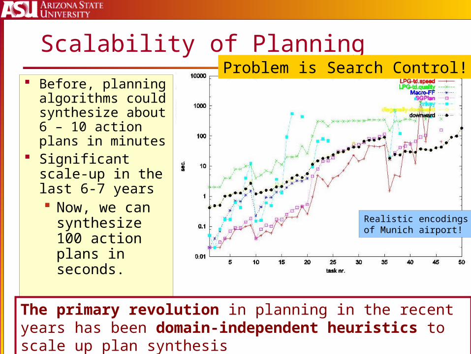
Scalability of Planning
Before, planning algorithms could synthesize about 6 – 10 action plans in minutes
Significant scale-up in the last 6-7 years Now, we can
synthesize 100 action plans in seconds.
Realistic encodings of Munich airport!
The primary revolution in planning in the recent years has been domain-independent heuristics to scale up plan synthesis
Problem is Search Control!!!
June 7th, 2006 ICAPS'06 Tutorial T6 4
Motivation
Ways to improve Planner Scalability Problem Formulation Search Space Reachability Heuristics
Domain (Formulation) Independent Work for many search spaces Flexible – work with most domain features Overall complement other scalability techniques Effective!!
June 7th, 2006 ICAPS'06 Tutorial T6 5
Topics
Classical Planning Cost Based Planning Partial Satisfaction Planning <Break> Non-Deterministic/Probabilistic Planning Resources (Continuous Quantities) Temporal Planning Hybrid Models Wrap-up Rao
Rao
Dan
June 7th, 2006 ICAPS'06 Tutorial T6 6
Classical Planning
June 7th, 2006 ICAPS'06 Tutorial T6 7
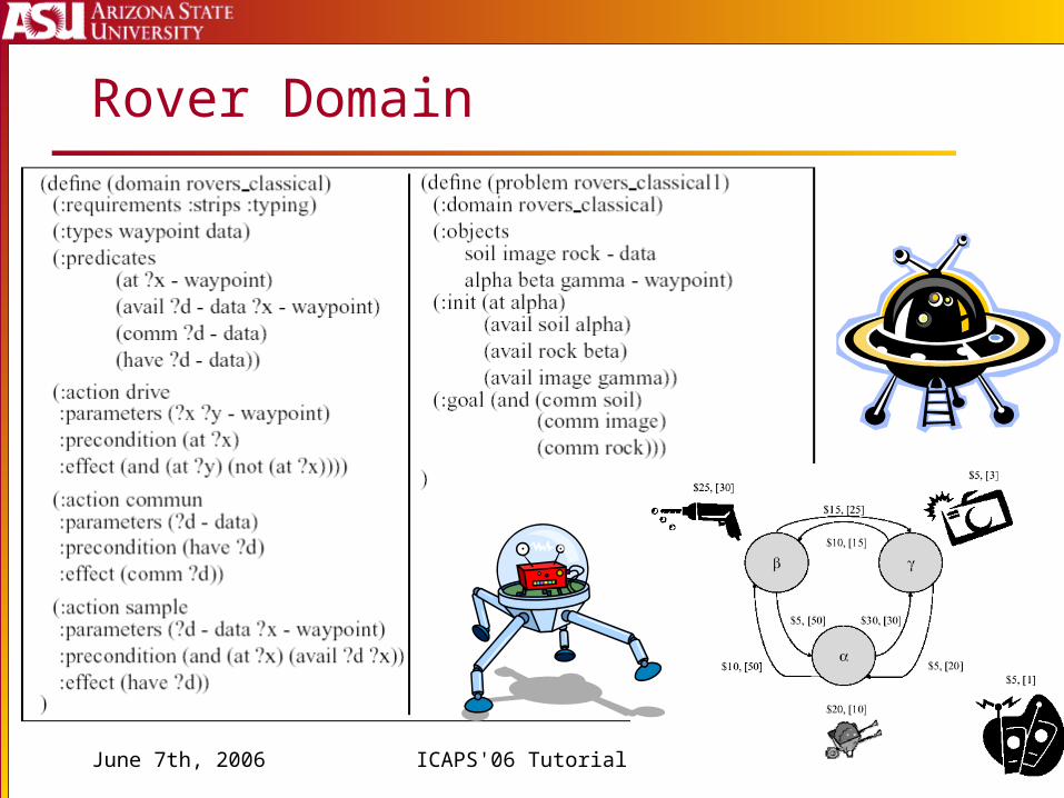
Rover Domain
June 7th, 2006 ICAPS'06 Tutorial T6 8
Classical Planning
Relaxed Reachability Analysis Types of Heuristics
Level-based Relaxed Plans
Mutexes Heuristic Search
Progression Regression Plan Space
Exploiting Heuristics
June 7th, 2006 ICAPS'06 Tutorial T6 9
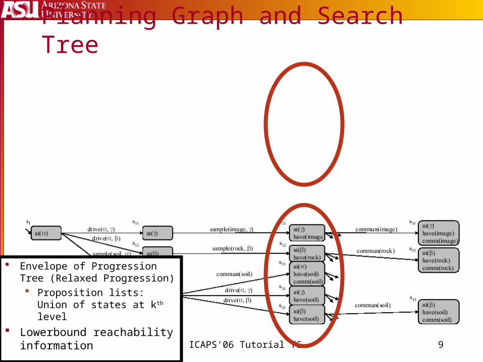
Planning Graph and Search Tree
Envelope of Progression Tree (Relaxed Progression) Proposition lists: Union of
states at kth level
Lowerbound reachability information
June 7th, 2006 ICAPS'06 Tutorial T6 10
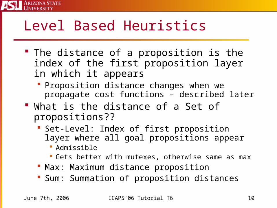
Level Based Heuristics
The distance of a proposition is the index of the first proposition layer in which it appears Proposition distance changes when we propagate cost
functions – described later What is the distance of a Set of propositions??
Set-Level: Index of first proposition layer where all goal propositions appear Admissible Gets better with mutexes, otherwise same as max
Max: Maximum distance proposition Sum: Summation of proposition distances
June 7th, 2006 ICAPS'06 Tutorial T6 11
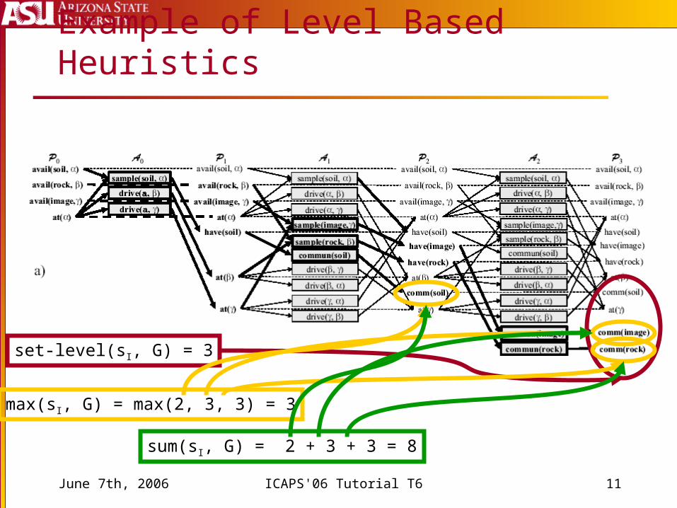
Example of Level Based Heuristics
set-level(sI, G) = 3
max(sI, G) = max(2, 3, 3) = 3
sum(sI, G) = 2 + 3 + 3 = 8
June 7th, 2006 ICAPS'06 Tutorial T6 12
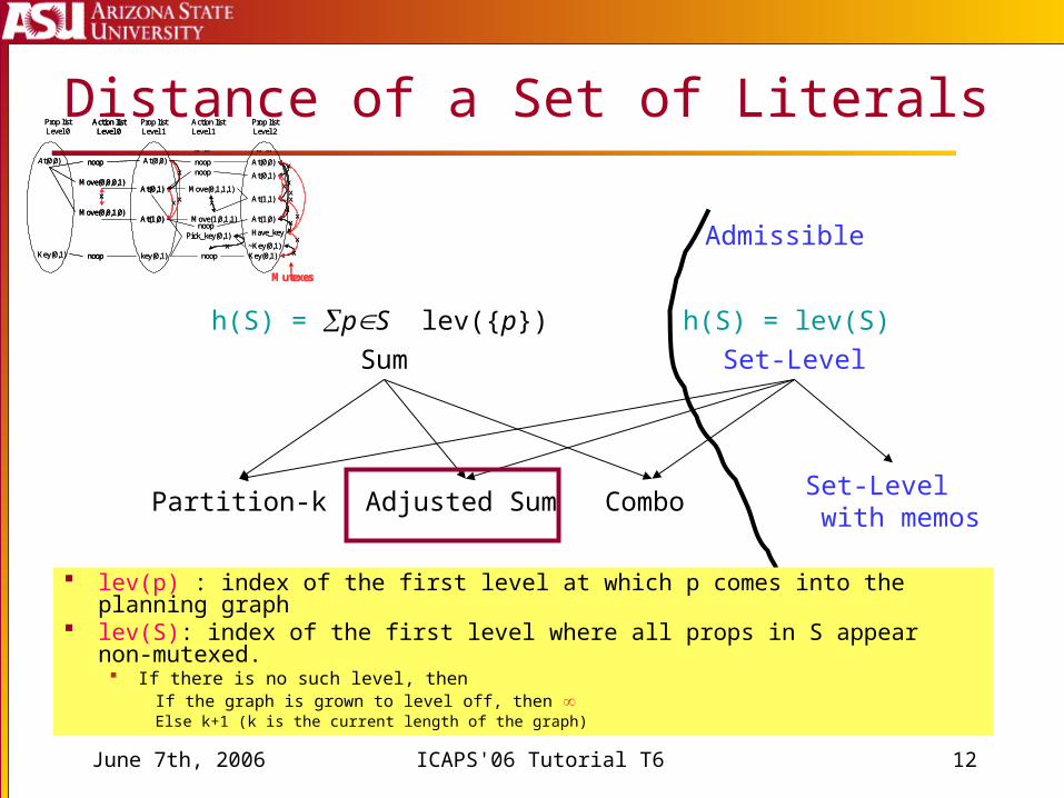
Distance of a Set of Literals
Sum Set-Level
Partition-k Adjusted Sum ComboSet-Level with memos
h(S) = pS lev({p}) h(S) = lev(S)
Admissible
At(0,0)
Key(0,1)
Prop listLevel 0
At(0,0)
Key(0,1)
Prop listLevel 0
At(0,1)
At(1,0)
noop
noop
Action listLevel 0
Move(0,0,0,1)
Move(0,0,1,0)
x
At(0,0)
key(0,1)
Prop listLevel 1
x
At(0,1)
At(1,0)
noop
noop
Action listLevel 0
Move(0,0,0,1)
Move(0,0,1,0)
xAt(0,1)
At(1,0)
noop
noop
Action listLevel 0
Move(0,0,0,1)
Move(0,0,1,0)
x
At(0,0)
key(0,1)
Prop listLevel 1
x
At(0,0)
Key(0,1)
noop
noop
x
Action listLevel 1
x
Prop listLevel 2
Move(0,1,1,1)At(1,1)
At(1,0)
At(0,1)
Move(1,0,1,1)
noop
noop
x
x
xx
xx
…...
x
…...
Pick_key(0,1) Have_key
~Key(0,1)xx
x
xx
Mutexes
At(0,0)
Key(0,1)
noop
noop
x
Action listLevel 1
x
Prop listLevel 2
Move(0,1,1,1)At(1,1)
At(1,0)
At(0,1)
Move(1,0,1,1)
noop
noop
x
x
xx
xx
…...
x
…...
Pick_key(0,1) Have_key
~Key(0,1)xx
x
xx
Mutexes
lev(p) : index of the first level at which p comes into the planning graph lev(S): index of the first level where all props in S appear non-mutexed.
If there is no such level, thenIf the graph is grown to level off, then Else k+1 (k is the current length of the graph)
June 7th, 2006 ICAPS'06 Tutorial T6 13
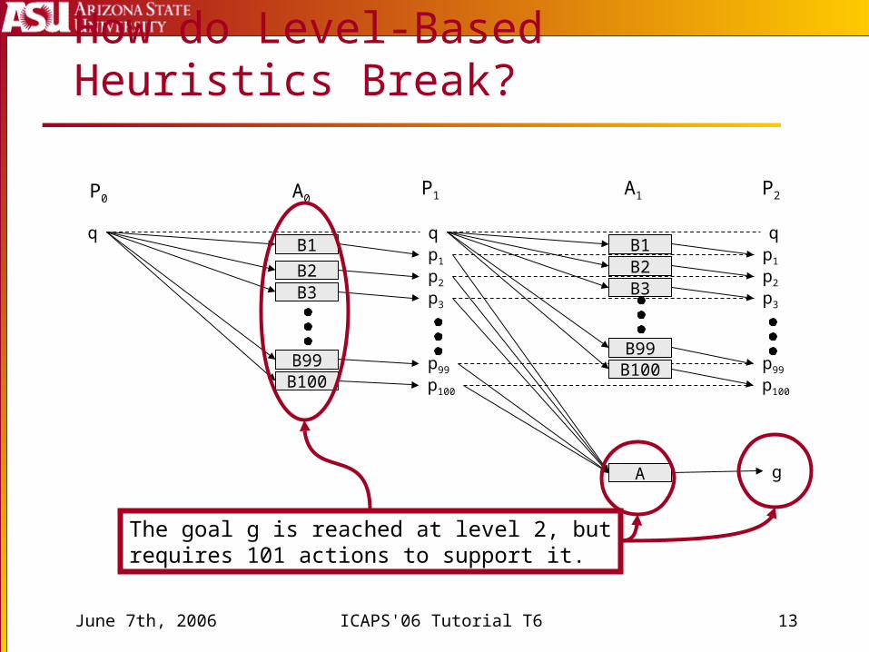
How do Level-Based Heuristics Break?
gA
p1
p2
p3
p99
p100
p1
p2
p3
p99
p100
B1q
B2B3
B99B100
q qB1B2B3
B99B100
A1P1 P2A0P0
The goal g is reached at level 2, butrequires 101 actions to support it.
June 7th, 2006 ICAPS'06 Tutorial T6 14
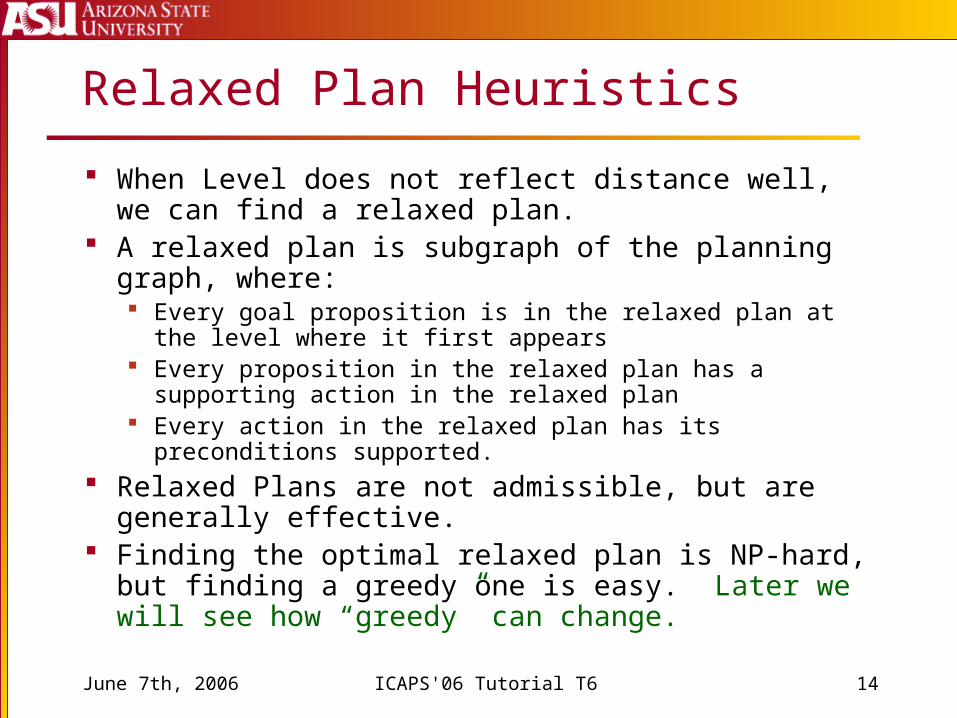
Relaxed Plan Heuristics
When Level does not reflect distance well, we can find a relaxed plan.
A relaxed plan is subgraph of the planning graph, where: Every goal proposition is in the relaxed plan at the level where it
first appears Every proposition in the relaxed plan has a supporting action in
the relaxed plan Every action in the relaxed plan has its preconditions supported.
Relaxed Plans are not admissible, but are generally effective.
Finding the optimal relaxed plan is NP-hard, but finding a greedy one is easy. Later we will see how “greedy” can change.
June 7th, 2006 ICAPS'06 Tutorial T6 15
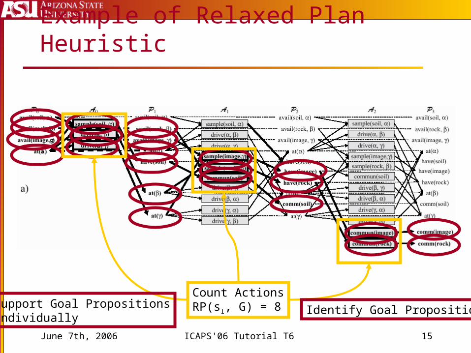
Example of Relaxed Plan Heuristic
Count ActionsRP(sI, G) = 8 Identify Goal PropositionsSupport Goal Propositions
Individually
June 7th, 2006 ICAPS'06 Tutorial T6 16
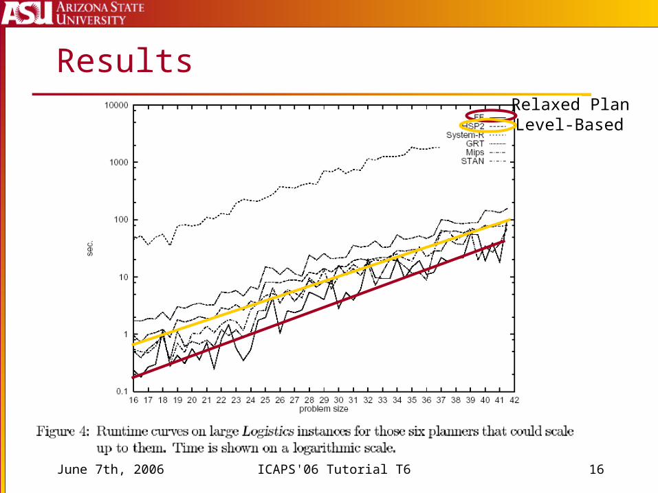
ResultsRelaxed PlanLevel-Based
June 7th, 2006 ICAPS'06 Tutorial T6 17
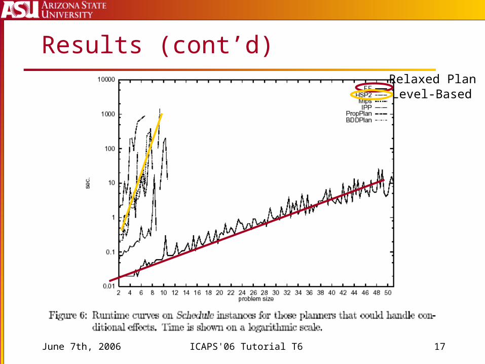
Results (cont’d)Relaxed PlanLevel-Based
June 7th, 2006 ICAPS'06 Tutorial T6 18
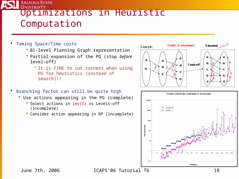
Optimizations in Heuristic Computation
Taming Space/Time costs Bi-level Planning Graph representation Partial expansion of the PG (stop before level-
off) It is FINE to cut corners when using PG for
heuristics (instead of search)!!
Branching factor can still be quite high Use actions appearing in the PG (complete)
Select actions in lev(S) vs Levels-off (incomplete) Consider action appearing in RP (incomplete)
Heuristic extracted from partial graph vs. leveled graph
0.1
1
10
100
1000
10000
100000
1 11 21 31 41 51 61 71 81 91 101 111 121 131 141 151 161
Problems
Tim
e(S
eco
nd
s)
Levels-off
Lev(S)
•A •A•A •A
•B•B
•C
•B
•C
•D
•B
•C
•D
•E
•A
•B
•C
•D
•E
x x
x
x
x
x
xxx
•A •A•A •A
•B•B
•C
•B
•C
•D
•B
•C
•D
•E
•A
•B
•C
•D
•E
x x
x
x
x
x
xxx
Goals C,D are presentExample: Levels off
Trade-off
Discarded
June 7th, 2006 ICAPS'06 Tutorial T6 19
Adjusting for Negative Interactions
Until now we assumed actions only positively interact. What about negative interactions?
Mutexes help us capture some negative interactions Types
Actions: Interference/Competing Needs Propositions: Inconsistent Support
Binary are the most common and practical |A| + 2|P|-ary will allow us to solve the planning
problem with a backtrack-free GraphPlan search An action layer may have |A| actions and 2|P| noops
Serial Planning Graph assumes all non-noop actions are mutex
June 7th, 2006 ICAPS'06 Tutorial T6 20
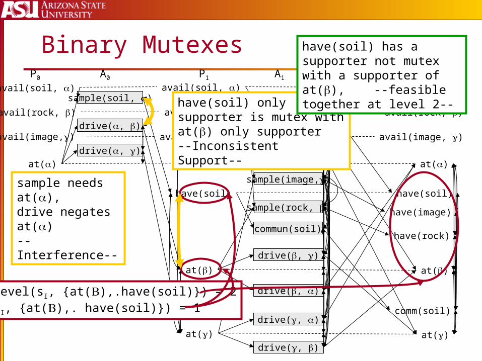
Binary Mutexes
at()
sample(soil, )
drive(, )
drive(, )
avail(soil, )
avail(rock, )
avail(image,)
at()
avail(soil, )
avail(rock, )
avail(image, )
at()
at()
have(soil)
sample(soil, )
drive(, )
drive(, )at()
avail(soil, )
avail(rock, )
avail(image, )
at()
at()
have(soil)
drive(, )
drive(, )
drive(, )
commun(soil)
sample(rock, )
sample(image,)
drive(, )
have(image)
comm(soil)
have(rock)
A1A0 P1P0 P2
Set-Level(sI, {at(),.have(soil)}) = 2Max(sI, {at(),. have(soil)}) = 1
sample needs at(),drive negates at()--Interference--
have(soil) only supporter is mutex with at() only supporter --Inconsistent Support--
have(soil) has a supporter not mutex with a supporter of at(), --feasible together at level 2--
June 7th, 2006 ICAPS'06 Tutorial T6 21
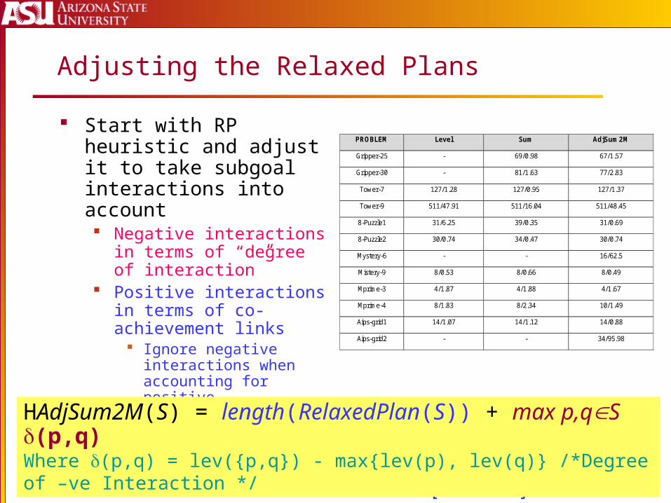
Adjusting the Relaxed Plans
Start with RP heuristic and adjust it to take subgoal interactions into account Negative interactions in terms
of “degree of interaction” Positive interactions in terms
of co-achievement links Ignore negative interactions
when accounting for positive interactions (and vice versa)
PROBLEM Level Sum AdjSum2M
Gripper-25 - 69/0.98 67/1.57
Gripper-30 - 81/1.63 77/2.83
Tower-7 127/1.28 127/0.95 127/1.37
Tower-9 511/47.91 511/16.04 511/48.45
8-Puzzle1 31/6.25 39/0.35 31/0.69
8-Puzzle2 30/0.74 34/0.47 30/0.74
Mystery-6 - - 16/62.5
Mistery-9 8/0.53 8/0.66 8/0.49
Mprime-3 4/1.87 4/1.88 4/1.67
Mprime-4 8/1.83 8/2.34 10/1.49
Aips-grid1 14/1.07 14/1.12 14/0.88
Aips-grid2 - - 34/95.98
[AAAI 2000]
HAdjSum2M(S) = length(RelaxedPlan(S)) + max p,qS (p,q)Where (p,q) = lev({p,q}) - max{lev(p), lev(q)} /*Degree of –ve Interaction */
June 7th, 2006 ICAPS'06 Tutorial T6 22
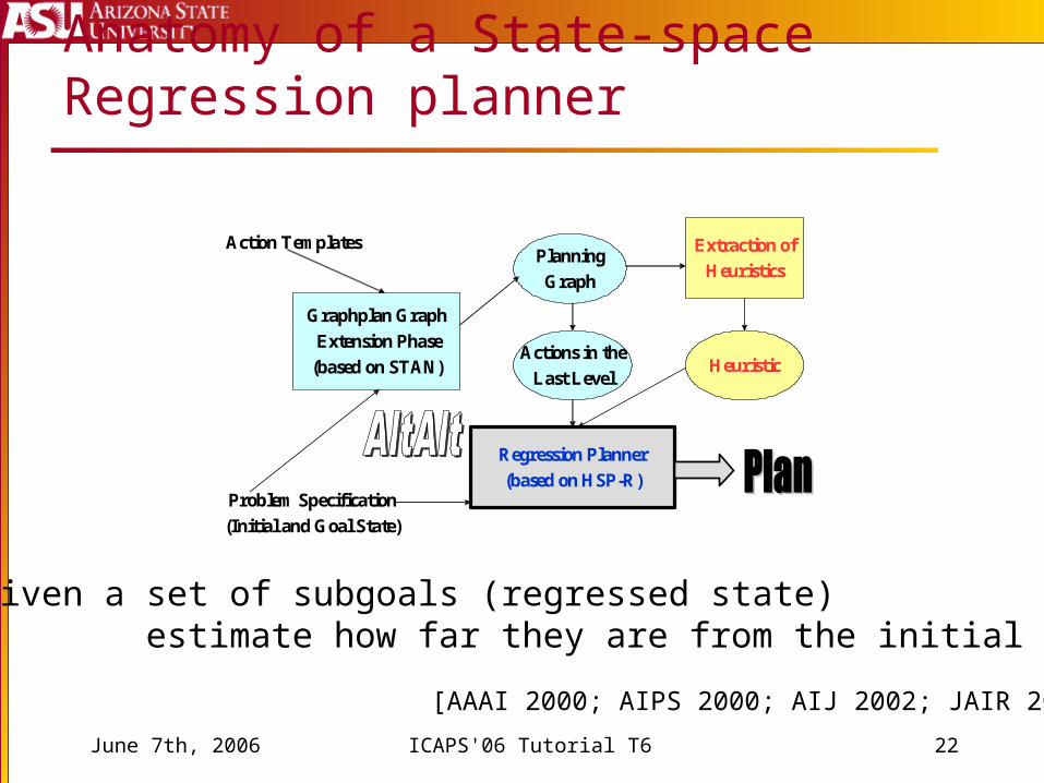
Anatomy of a State-space Regression planner
[AAAI 2000; AIPS 2000; AIJ 2002; JAIR 2003]
Problem: Given a set of subgoals (regressed state) estimate how far they are from the initial state
Graphplan Graph
Extension Phase
(based on STAN)
Planning
Graph
Actions in the
Last Level
Action Templates Extraction of
Heuristics
Heuristic
Regression Planner
(based on HSP-R)Problem Specification
(Initial and Goal State)
June 7th, 2006 ICAPS'06 Tutorial T6 23
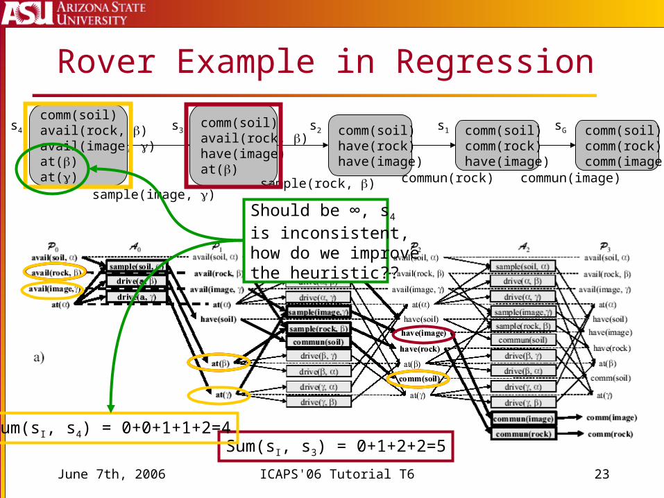
Rover Example in Regression
comm(soil)comm(rock)comm(image)
commun(image)
comm(soil)comm(rock)have(image)
comm(soil)have(rock)have(image)
comm(soil)avail(rock, )have(image)at()
sample(rock, ) commun(rock)
comm(soil)avail(rock, )avail(image, )at()at()
sample(image, )
sGs1s2s3s4
Sum(sI, s3) = 0+1+2+2=5Sum(sI, s4) = 0+0+1+1+2=4
Should be ∞, s4 is inconsistent,how do we improvethe heuristic??
June 7th, 2006 ICAPS'06 Tutorial T6 24
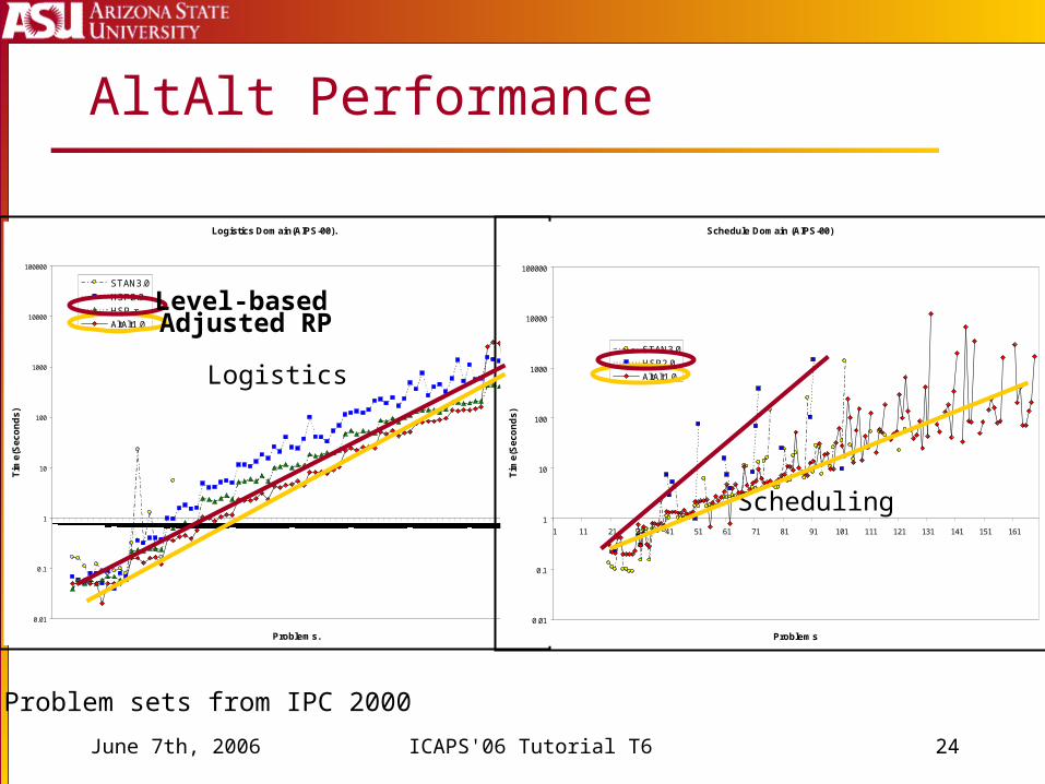
AltAlt Performance
Logistics Domain(AIPS-00).
0.01
0.1
1
10
100
1000
10000
100000
Problems.
Tim
e(S
eco
nd
s)
STAN3.0
HSP2.0
HSP-r
AltAlt1.0
Schedule Domain (AIPS-00)
0.01
0.1
1
10
100
1000
10000
100000
1 11 21 31 41 51 61 71 81 91 101 111 121 131 141 151 161
Problems
Tim
e(S
ec
on
ds
)
STAN3.0
HSP2.0
AltAlt1.0Logistics
Scheduling
Problem sets from IPC 2000
Adjusted RPLevel-based
June 7th, 2006 ICAPS'06 Tutorial T6 25
In the beginning it was all POP.
Then it was cruellyUnPOPped
The good timesreturn with Re(vived)POP
Plan Space Search
June 7th, 2006 ICAPS'06 Tutorial T6 26
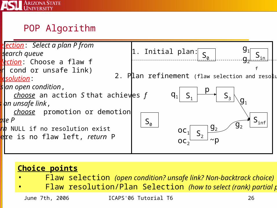
POP Algorithm
1. Plan Selection: Select a plan P from the search queue2. Flaw Selection: Choose a flaw f
(open cond or unsafe link)3. Flaw resolution:
If f is an open condition, choose an action S that achieves f If f is an unsafe link, choose promotion or demotion Update P Return NULL if no resolution exist
4. If there is no flaw left, return P
S0
S1
S2
S3
Sinf
p
~p
g1
g2g2oc1
oc2
q1
Choice points• Flaw selection (open condition? unsafe link? Non-backtrack choice)• Flaw resolution/Plan Selection (how to select (rank) partial plan?)
S0
Sinf
g1
g2
1. Initial plan:
2. Plan refinement (flaw selection and resolution):
June 7th, 2006 ICAPS'06 Tutorial T6 27
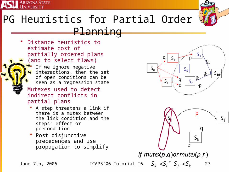
Distance heuristics to estimate cost of partially ordered plans (and to select flaws) If we ignore negative
interactions, then the set of open conditions can be seen as a regression state
Mutexes used to detect indirect conflicts in partial plans A step threatens a link if there is
a mutex between the link condition and the steps’ effect or precondition
Post disjunctive precedences and use propagation to simplify
PG Heuristics for Partial Order Planning
Si
Sk
Sj
p
q
r
S0
S1
S2
S3p
~p
g1
g2g2q
r
q1
Sinf
S4
S5
kjik SSSS
rpmutexorqpmutexif
),(),(
June 7th, 2006 ICAPS'06 Tutorial T6 28
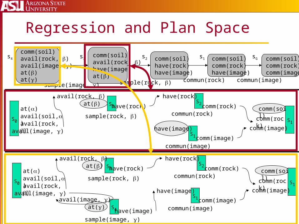
Regression and Plan Space
comm(soil)comm(rock)comm(image)
commun(image)
comm(soil)comm(rock)have(image)
comm(soil)have(rock)have(image)
comm(soil)avail(rock, )have(image)at()
sample(rock, )
S1comm(rock)
comm(image)
comm(soil)
S0 avail(rock,)avail(image, )
avail(soil,)at()
commun(image)
S1 comm(image)
have(image)
commun(rock)
S2 comm(rock)
have(rock)
sample(rock, )
S3 have(rock)
avail(rock, )at()
commun(rock)
comm(soil)avail(rock, )avail(image, )at()at()
sample(image, )
sample(image, )
S4 have(image)
avail(image, )at()
S1comm(rock)
comm(image)
comm(soil)
S0 avail(rock,)avail(image, )
avail(soil,)at()
commun(image)
S1 comm(image)
have(image)
commun(rock)
S2 comm(rock)
have(rock)
sample(rock, )
S3 have(rock)
avail(rock, )at()
sGs1s2s3s4
June 7th, 2006 ICAPS'06 Tutorial T6 29
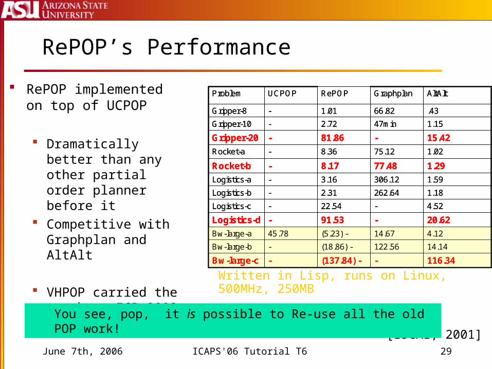
RePOP’s Performance
4.1214.67(5.23) -45.78Bw-large-a
14.14122.56(18.86) --Bw-large-b
116.34-(137.84) --Bw-large-c
20.62-91.53-Logistics-d
4.52-22.54-Logistics-c
1.18262.642.31-Logistics-b
1.59306.123.16-Logistics-a
1.2977.488.17-Rocket-b
1.0275.128.36-Rocket-a
15.42-81.86-Gripper-20
1.1547min2.72-Gripper-10
.4366.821.01-Gripper-8
AltAltGraphplanRePOPUCPOPProblem
4.1214.67(5.23) -45.78Bw-large-a
14.14122.56(18.86) --Bw-large-b
116.34-(137.84) --Bw-large-c
20.62-91.53-Logistics-d
4.52-22.54-Logistics-c
1.18262.642.31-Logistics-b
1.59306.123.16-Logistics-a
1.2977.488.17-Rocket-b
1.0275.128.36-Rocket-a
15.42-81.86-Gripper-20
1.1547min2.72-Gripper-10
.4366.821.01-Gripper-8
AltAltGraphplanRePOPUCPOPProblem RePOP implemented on top of UCPOP
Dramatically better than any other partial order planner before it
Competitive with Graphplan and AltAlt
VHPOP carried the torch at ICP 2002
[IJCAI, 2001]
You see, pop, it is possible to Re-use all the old POP work!
Written in Lisp, runs on Linux, 500MHz, 250MB
June 7th, 2006 ICAPS'06 Tutorial T6 30
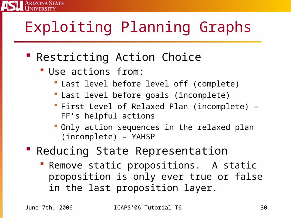
Exploiting Planning Graphs
Restricting Action Choice Use actions from:
Last level before level off (complete) Last level before goals (incomplete) First Level of Relaxed Plan (incomplete) – FF’s helpful
actions Only action sequences in the relaxed plan (incomplete) –
YAHSP
Reducing State Representation Remove static propositions. A static proposition is
only ever true or false in the last proposition layer.
June 7th, 2006 ICAPS'06 Tutorial T6 31
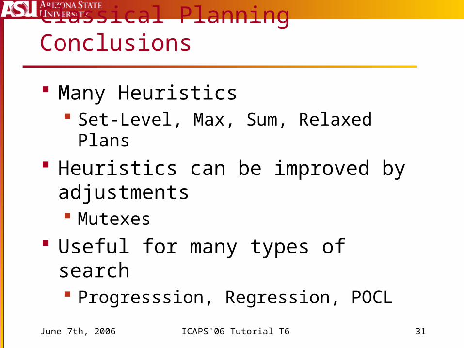
Classical Planning Conclusions
Many Heuristics Set-Level, Max, Sum, Relaxed Plans
Heuristics can be improved by adjustments Mutexes
Useful for many types of search Progresssion, Regression, POCL
June 7th, 2006 ICAPS'06 Tutorial T6 32
Cost-Based Planning
June 7th, 2006 ICAPS'06 Tutorial T6 33
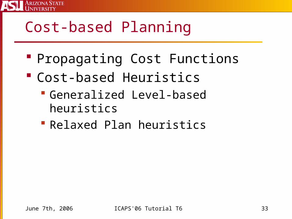
Cost-based Planning
Propagating Cost Functions Cost-based Heuristics
Generalized Level-based heuristics Relaxed Plan heuristics
June 7th, 2006 ICAPS'06 Tutorial T6 34
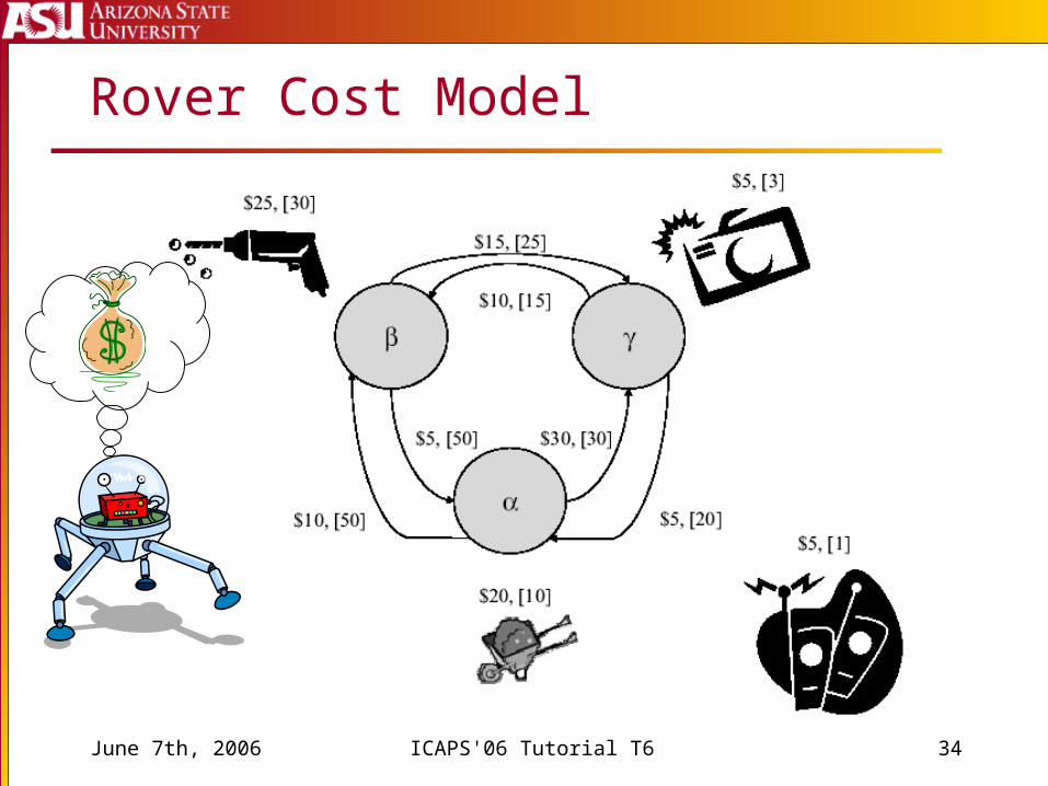
Rover Cost Model
June 7th, 2006 ICAPS'06 Tutorial T6 35
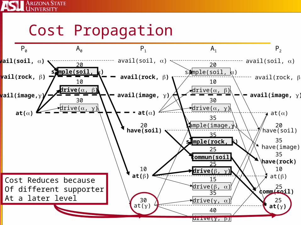
Cost Propagation
at()
sample(soil, )
drive(, )
drive(, )
avail(soil, )
avail(rock, )
avail(image,)
at()
avail(soil, )
avail(rock, )
avail(image, )
at()
at()
have(soil)
sample(soil, )
drive(, )
drive(, )at()
avail(soil, )
avail(rock, )
avail(image, )
at()
at()
have(soil)
drive(, )
drive(, )
drive(, )
commun(soil)
sample(rock, )
sample(image,)
drive(, )
have(image)
comm(soil)
have(rock)
20
10
30
20
10
30
2035
10
30
35
25
25
15
35
40
20
35
35
10
25
25
A1A0 P1P0 P2
Cost Reduces becauseOf different supporterAt a later level
June 7th, 2006 ICAPS'06 Tutorial T6 36
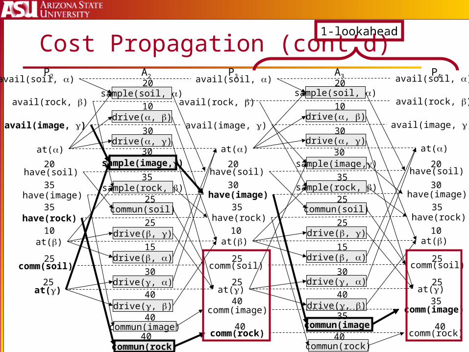
at()
Cost Propagation (cont’d)avail(soil, )
avail(rock, )
avail(image, )
at()
at()
have(soil)
have(image)
comm(soil)
have(rock)
commun(image)
commun(rock)
comm(image)
comm(rock)
sample(soil, )
drive(, )
drive(, )at()
avail(soil, )
avail(rock, )
avail(image, )
at()
at()
have(soil)
drive(, )
drive(, )
drive(, )
commun(soil)
sample(rock, )
sample(image,)
drive(, )
have(image)
comm(soil)
have(rock)
commun(image)
commun(rock)
comm(image)
comm(rock)
sample(soil, )
drive(, )
drive(, )at()
avail(soil, )
avail(rock, )
avail(image, )
at()
at()
have(soil)
drive(, )
drive(, )
drive(, )
commun(soil)
sample(rock, )
sample(image,)
drive(, )
have(image)
comm(soil)
have(rock)
20
10
30
20
10
30
20 20 20
35
35
10 10 10
25
25
30
35 35
35 35
4040 40
40
25 253030
40 40
40
40
15
25
25 25
25 25
30
30
30
25
15
35
35
A2P2 P3 A3 P4
1-lookahead
June 7th, 2006 ICAPS'06 Tutorial T6 37
Terminating Cost Propagation
Stop when: goals are reached (no-lookahead) costs stop changing (∞-lookahead) k levels after goals are reached (k-lookahead)
June 7th, 2006 ICAPS'06 Tutorial T6 38
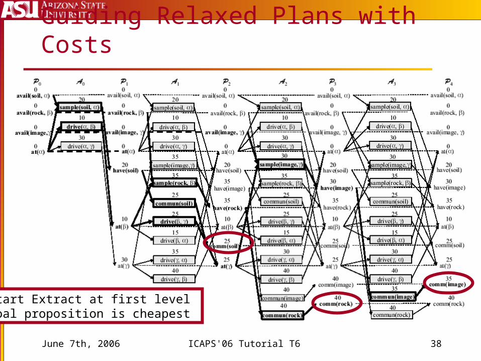
Guiding Relaxed Plans with Costs
Start Extract at first level goal proposition is cheapest
June 7th, 2006 ICAPS'06 Tutorial T6 39
Cost-Based Planning Conclusions
Cost-Functions: Remove false assumption that level is
correlated with cost Improve planning with non-uniform cost
actions Are cheap to compute (constant overhead)
June 7th, 2006 ICAPS'06 Tutorial T6 40
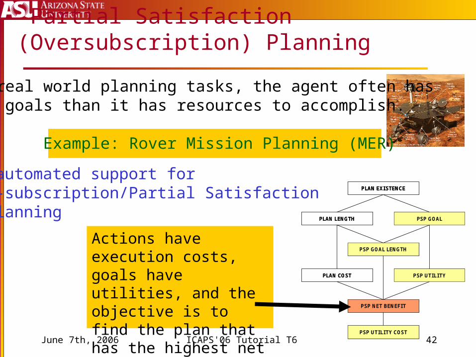
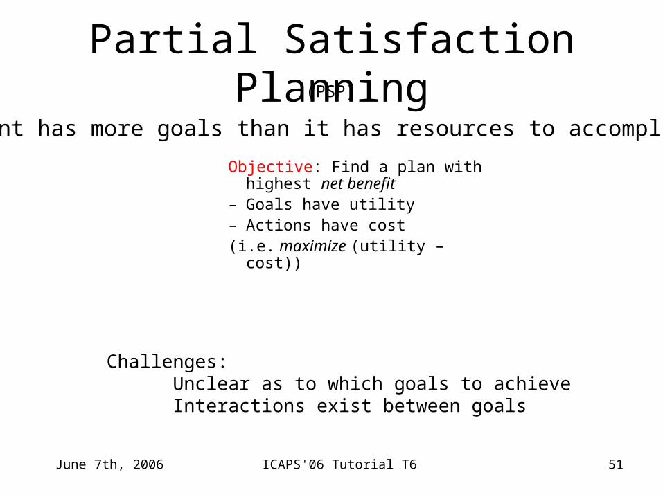
Partial Satisfaction (Over-Subscription) Planning
June 7th, 2006 ICAPS'06 Tutorial T6 41
Partial Satisfaction Planning
Selecting Goal Sets Estimating goal benefit
Anytime goal set selection Adjusting for negative interactions between
goals
June 7th, 2006 ICAPS'06 Tutorial T6 42
Actions have execution costs, goals have utilities, and the objective is to find the plan that has the highest net benefit.
Partial Satisfaction (Oversubscription) Planning
In many real world planning tasks, the agent often has more goals than it has resources to accomplish.
Example: Rover Mission Planning (MER)
Need automated support for Over-subscription/Partial Satisfaction Planning
PLAN EXISTENCE
PLAN LENGTH
PSP GOAL LENGTH
PSP GOAL
PLAN COST PSP UTILITY
PSP UTILITY COST
PSP NET BENEFIT
PLAN EXISTENCE
PLAN LENGTH
PSP GOAL LENGTH
PSP GOAL
PLAN COST PSP UTILITY
PSP UTILITY COST
PSP NET BENEFIT
June 7th, 2006 ICAPS'06 Tutorial T6 43
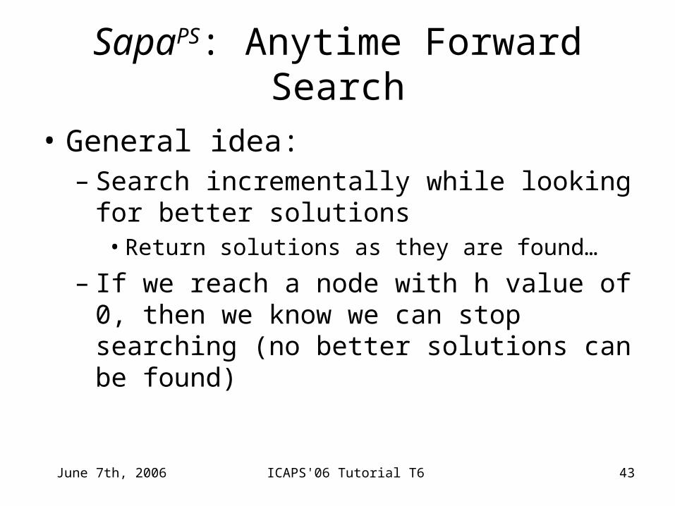
SapaPS: Anytime Forward Search
• General idea:– Search incrementally while looking for better
solutions• Return solutions as they are found…
– If we reach a node with h value of 0, then we know we can stop searching (no better solutions can be found)
June 7th, 2006 ICAPS'06 Tutorial T6 44
Background: Cost Propagation
at()
sample(soil, )
drive(, )
drive(, )at()
avail(soil, )
avail(rock, )
avail(image, )
at()
at()
have(soil)
sample(soil, )
drive(, )
drive(, )at()
avail(soil, )
avail(rock, )
avail(image, )
at()
at()
have(soil)
drive(, )
drive(, )
drive(, )
commun(soil)
sample(rock, )
sample(image,)
drive(, )
have(image)
comm(soil)
have(rock)
20
10
30
20
10
30
2035
10
30
35
25
25
15
35
40
20
35
35
10
25
25
A1A0 P1P0 P2
Cost Reduces becauseOf different supporterAt a later level
June 7th, 2006 ICAPS'06 Tutorial T6 45
Adapting PG heuristics for PSP Challenges:
Need to propagate costs on the planning graph
The exact set of goals are not clear Interactions between goals Obvious approach of considering all 2n goal
subsets is infeasible
Idea: Select a subset of the top level goals upfront
Challenge: Goal interactions Approach: Estimate the net benefit
of each goal in terms of its utility minus the cost of its relaxed plan
Bias the relaxed plan extraction to (re)use the actions already chosen for other goals
Action Templates
Problem Spec
(Init, Goal state)
Solution Plan
GraphplanPlan Extension Phase
(based on STAN)
+
Cost Propagation
Cost-sensitive PlanningGraph
Extraction ofHeuristics
HeuristicsActions in the
Last Level
Goal Set selection
Algorithm
Cost sensitive
Search
Action Templates
Problem Spec
(Init, Goal state)
Solution Plan
GraphplanPlan Extension Phase
(based on STAN)
+
Cost Propagation
Cost-sensitive PlanningGraph
Extraction ofHeuristics
HeuristicsActions in the
Last Level
Goal Set selection
Algorithm
Cost sensitive
Search
0
0
0
0
4
0
0
4
5 5
8
5 5
3
l=0 l=1 l=2
4 4
12
June 7th, 2006 ICAPS'06 Tutorial T6 46
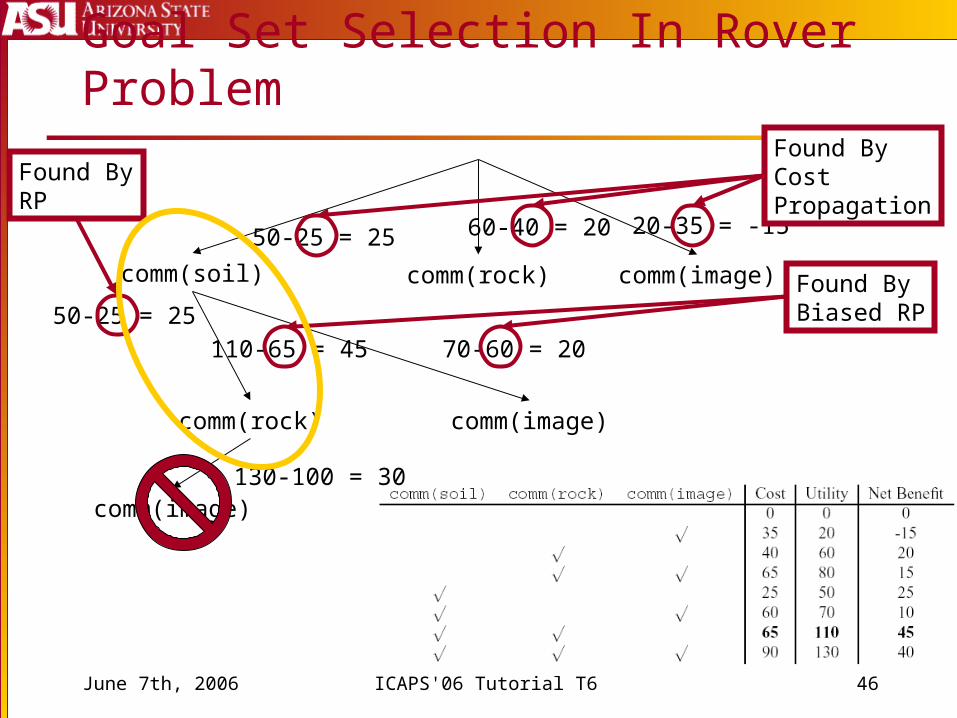
Goal Set Selection In Rover Problem
comm(soil) comm(rock) comm(image)
50-25 = 25 60-40 = 20 20-35 = -15
Found ByCost Propagation
comm(rock) comm(image)
50-25 = 25
Found ByRP
110-65 = 45
Found ByBiased RP
70-60 = 20
comm(image)130-100 = 30
June 7th, 2006 ICAPS'06 Tutorial T6 47
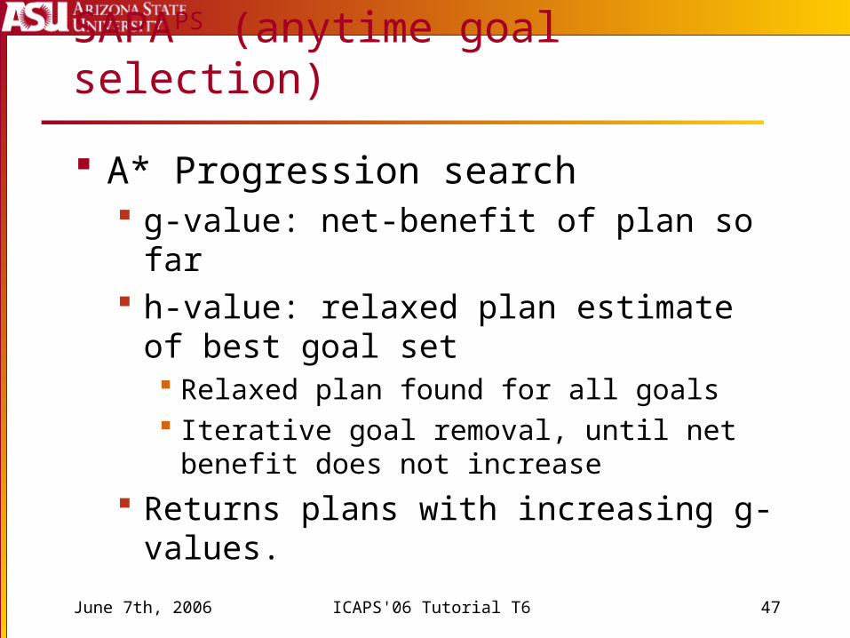
SAPAPS (anytime goal selection)
A* Progression search g-value: net-benefit of plan so far h-value: relaxed plan estimate of best goal set
Relaxed plan found for all goals Iterative goal removal, until net benefit does not
increase
Returns plans with increasing g-values.
June 7th, 2006 ICAPS'06 Tutorial T6 48
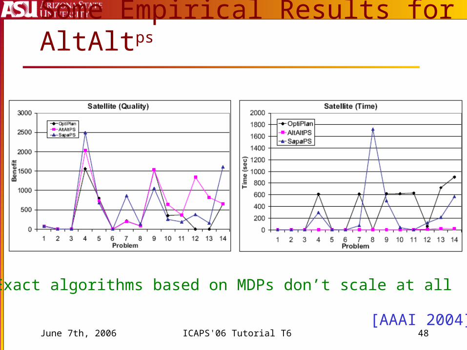
Some Empirical Results for AltAltps
[AAAI 2004]
Exact algorithms based on MDPs don’t scale at all
June 7th, 2006 ICAPS'06 Tutorial T6 49
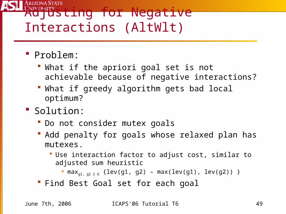
Adjusting for Negative Interactions (AltWlt)
Problem: What if the apriori goal set is not achievable because of
negative interactions? What if greedy algorithm gets bad local optimum?
Solution: Do not consider mutex goals Add penalty for goals whose relaxed plan has mutexes.
Use interaction factor to adjust cost, similar to adjusted sum heuristic
maxg1, g2 2 G {lev(g1, g2) – max(lev(g1), lev(g2)) }
Find Best Goal set for each goal
June 7th, 2006 ICAPS'06 Tutorial T6 50
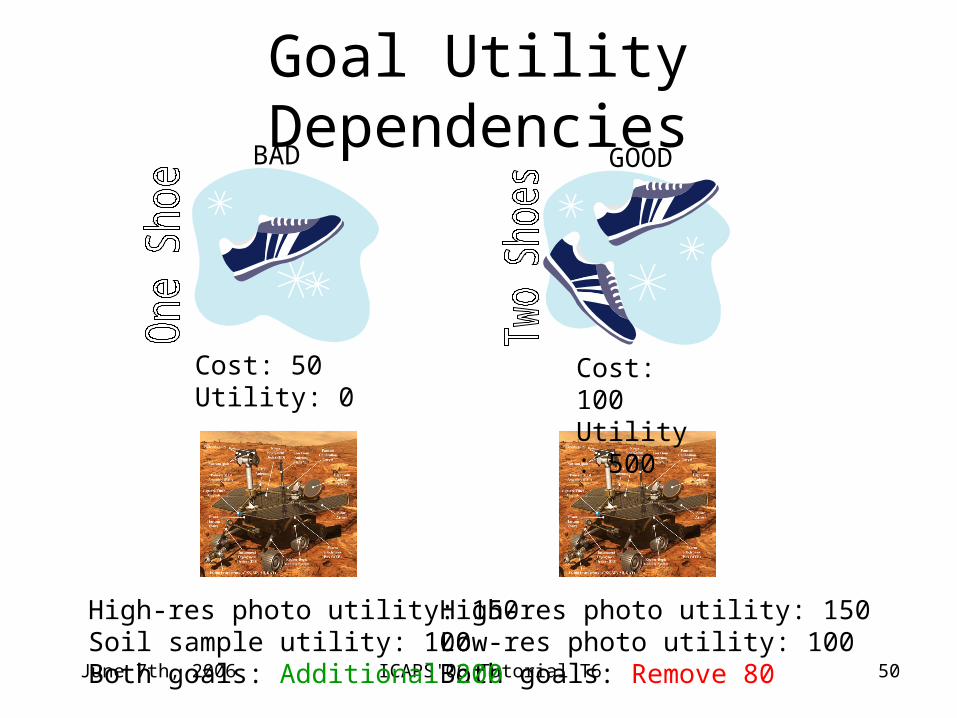
Goal Utility Dependencies
High-res photo utility: 150Low-res photo utility: 100Both goals: Remove 80
High-res photo utility: 150Soil sample utility: 100Both goals: Additional 200
Cost: 50Utility: 0
Cost: 100Utility: 500
BAD GOOD
June 7th, 2006 ICAPS'06 Tutorial T6 51
Partial Satisfaction Planning
Objective: Find a plan with highest net benefit
– Goals have utility – Actions have cost(i.e. maximize (utility – cost))
Agent has more goals than it has resources to accomplish
Challenges:Unclear as to which goals to achieveInteractions exist between goals
(PSP)
June 7th, 2006 ICAPS'06 Tutorial T6 52
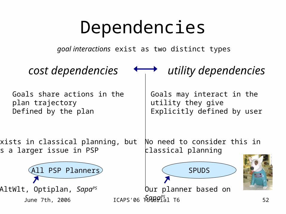
Dependencies
cost dependencies
Goals share actions in the plan trajectoryDefined by the plan
Goals may interact in the utility they giveExplicitly defined by user
utility dependencies
Exists in classical planning, butis a larger issue in PSP
No need to consider this inclassical planning
goal interactions exist as two distinct types
All PSP Planners SPUDS
Our planner based onSapaPS
AltWlt, Optiplan, SapaPS
June 7th, 2006 ICAPS'06 Tutorial T6 53
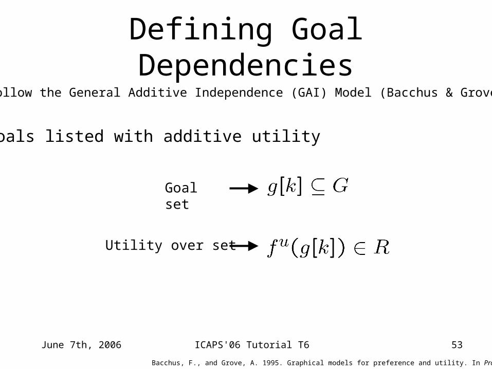
Defining Goal DependenciesFollow the General Additive Independence (GAI) Model (Bacchus & Grove)
Bacchus, F., and Grove, A. 1995. Graphical models for preference and utility. In Proc. of UAI-95.
Goals listed with additive utility
Goal set
Utility over set
June 7th, 2006 ICAPS'06 Tutorial T6 54
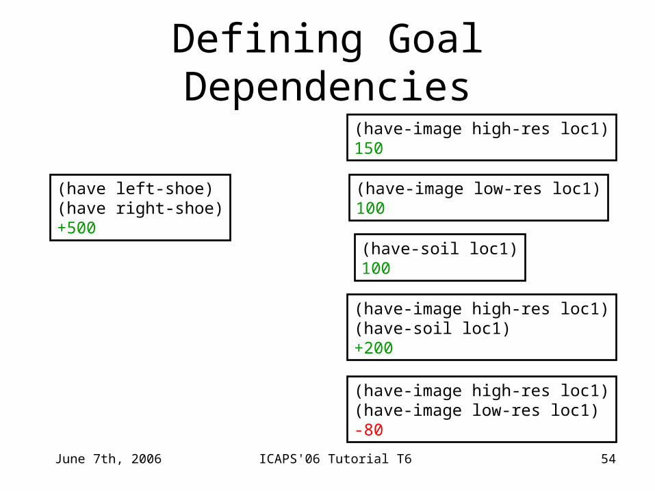
(have left-shoe)(have right-shoe)+500
(have-image low-res loc1)100
(have-image high-res loc1)(have-soil loc1)+200
Defining Goal Dependencies(have-image high-res loc1)150
(have-soil loc1)100
(have-image high-res loc1)(have-image low-res loc1)-80
June 7th, 2006 ICAPS'06 Tutorial T6 55
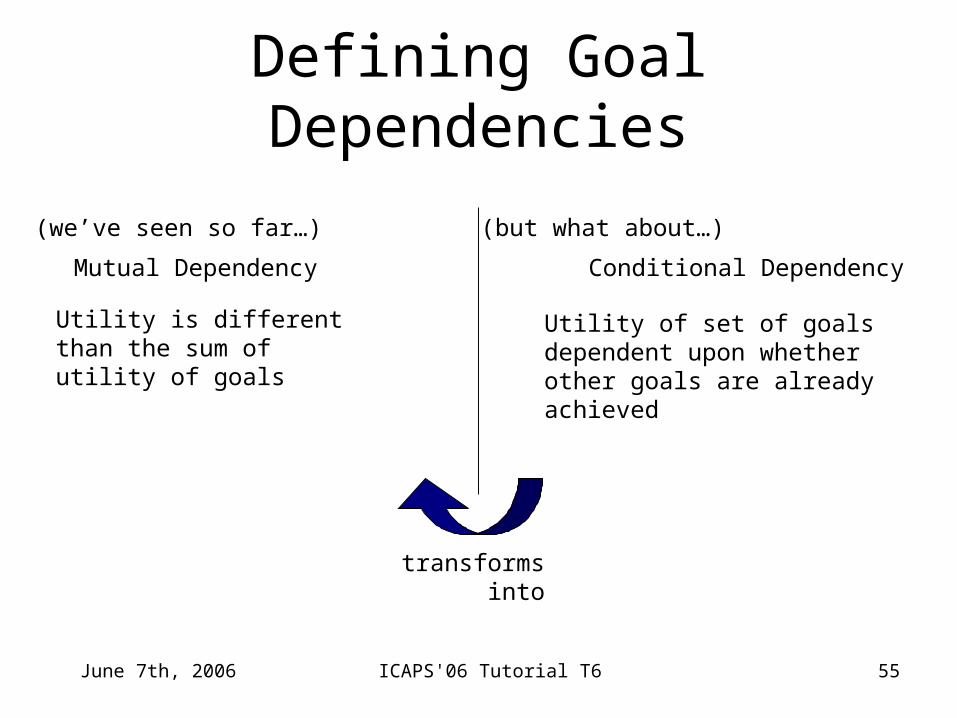
Defining Goal Dependencies
Mutual Dependency Conditional Dependency
Utility is different than the sum ofutility of goals
Utility of set of goals dependent upon whether other goals are already achieved
transforms into
(we’ve seen so far…) (but what about…)
June 7th, 2006 ICAPS'06 Tutorial T6 56
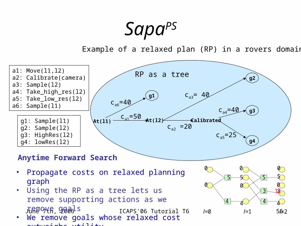
SapaPS
g2
g3
g4
a1: Move(l1,l2)a2: Calibrate(camera)a3: Sample(l2)a4: Take_high_res(l2)a5: Take_low_res(l2)a6: Sample(l1)
At(l1) At(l2) Calibratedca1=50
ca2 =20
ca3= 40
ca4=40
ca5=25
g1
ca6=40
Example of a relaxed plan (RP) in a rovers domain
RP as a tree
g1: Sample(l1)g2: Sample(l2)g3: HighRes(l2)g4: lowRes(l2)
• Propagate costs on relaxed planning graph• Using the RP as a tree lets us remove
supporting actions as we remove goals• We remove goals whose relaxed cost
outweighs utility
Anytime Forward Search0
0
0
0
4
0
0
4
5 5
8
5 5
3
l=0 l=1 l=2
4 4
12
June 7th, 2006 ICAPS'06 Tutorial T6 57
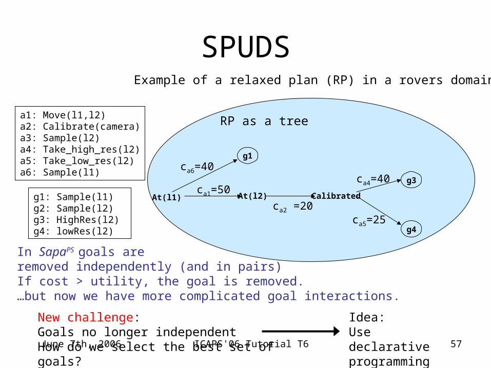
SPUDS
a1: Move(l1,l2)a2: Calibrate(camera)a3: Sample(l2)a4: Take_high_res(l2)a5: Take_low_res(l2)a6: Sample(l1)
At(l1) At(l2) Calibratedca1=50
ca2 =20
g1
ca6=40
RP as a tree
In SapaPS goals are removed independently (and in pairs)If cost > utility, the goal is removed.…but now we have more complicated goal interactions.
New challenge:Goals no longer independentHow do we select the best set of goals?
Idea:Use declarative programming
g1: Sample(l1)g2: Sample(l2)g3: HighRes(l2)g4: lowRes(l2)
g3ca4=40
g4ca5=25
Example of a relaxed plan (RP) in a rovers domain
June 7th, 2006 ICAPS'06 Tutorial T6 58
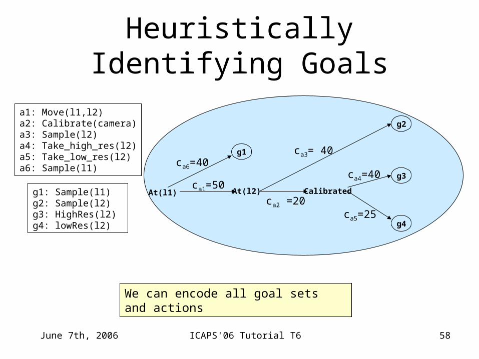
Heuristically Identifying Goals
g2
g3
g4
At(l1) At(l2) Calibratedca1=50
ca2 =20
ca3= 40
ca4=40
ca5=25
g1
ca6=40
a1: Move(l1,l2)a2: Calibrate(camera)a3: Sample(l2)a4: Take_high_res(l2)a5: Take_low_res(l2)a6: Sample(l1)
g1: Sample(l1)g2: Sample(l2)g3: HighRes(l2)g4: lowRes(l2)
We can encode all goal sets and actions
June 7th, 2006 ICAPS'06 Tutorial T6 59
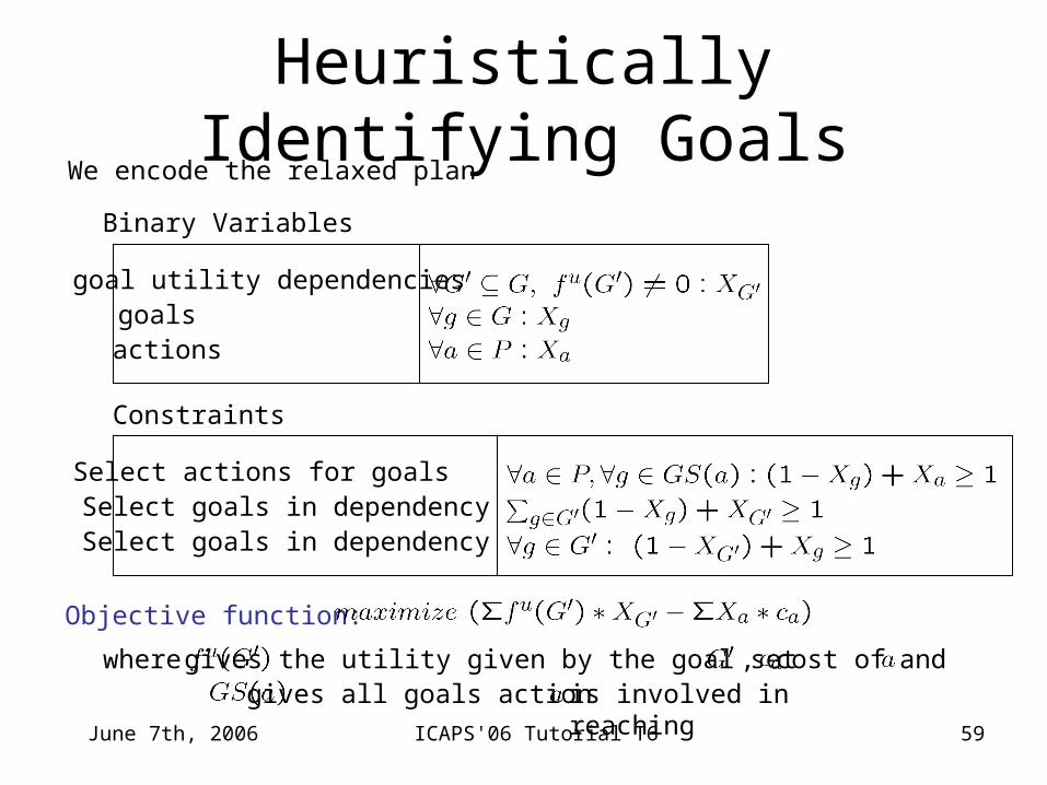
Heuristically Identifying Goals
goalsgoal utility dependencies
actions
Binary Variables
We encode the relaxed plan
Select goals in dependencySelect actions for goals
Select goals in dependency
Constraints
gives all goals action is involved in reaching
Objective function:
where gives the utility given by the goal set , cost of and
June 7th, 2006 ICAPS'06 Tutorial T6 60
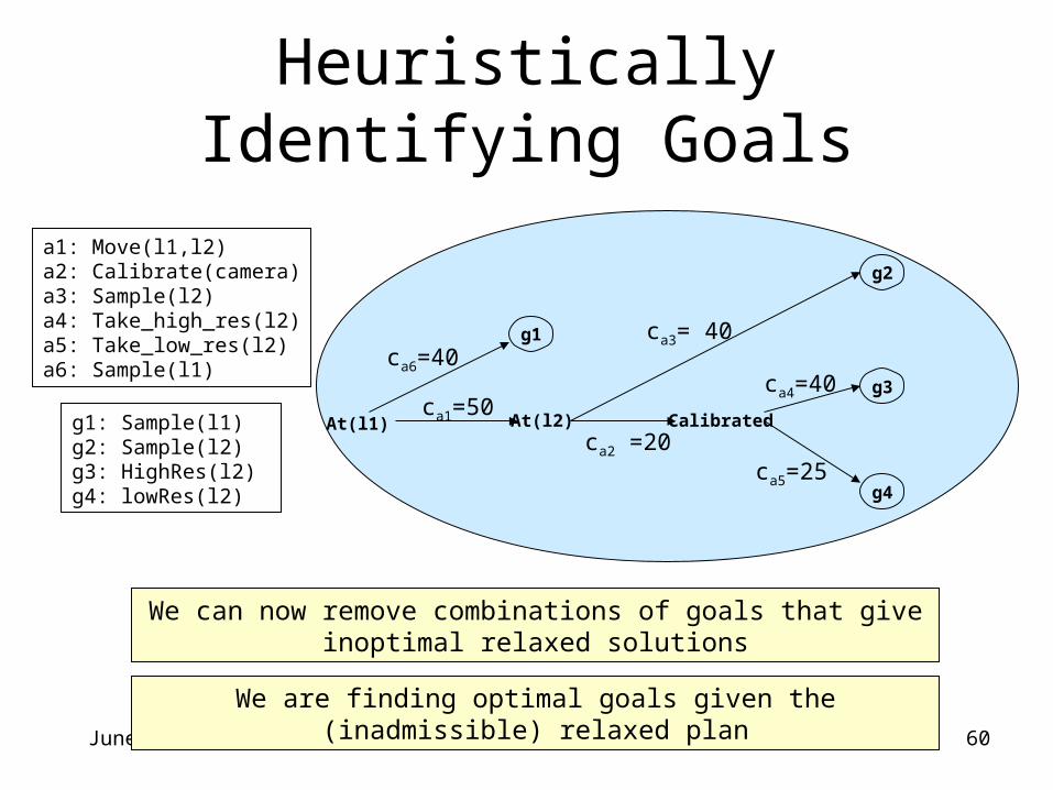
Heuristically Identifying Goals
g2
g3
g4
At(l1) At(l2) Calibratedca1=50
ca2 =20
ca3= 40
ca4=40
ca5=25
g1
ca6=40
a1: Move(l1,l2)a2: Calibrate(camera)a3: Sample(l2)a4: Take_high_res(l2)a5: Take_low_res(l2)a6: Sample(l1)
g1: Sample(l1)g2: Sample(l2)g3: HighRes(l2)g4: lowRes(l2)
We can now remove combinations of goals that give inoptimal relaxed solutions
We are finding optimal goals given the (inadmissible) relaxed plan
June 7th, 2006 ICAPS'06 Tutorial T6 61
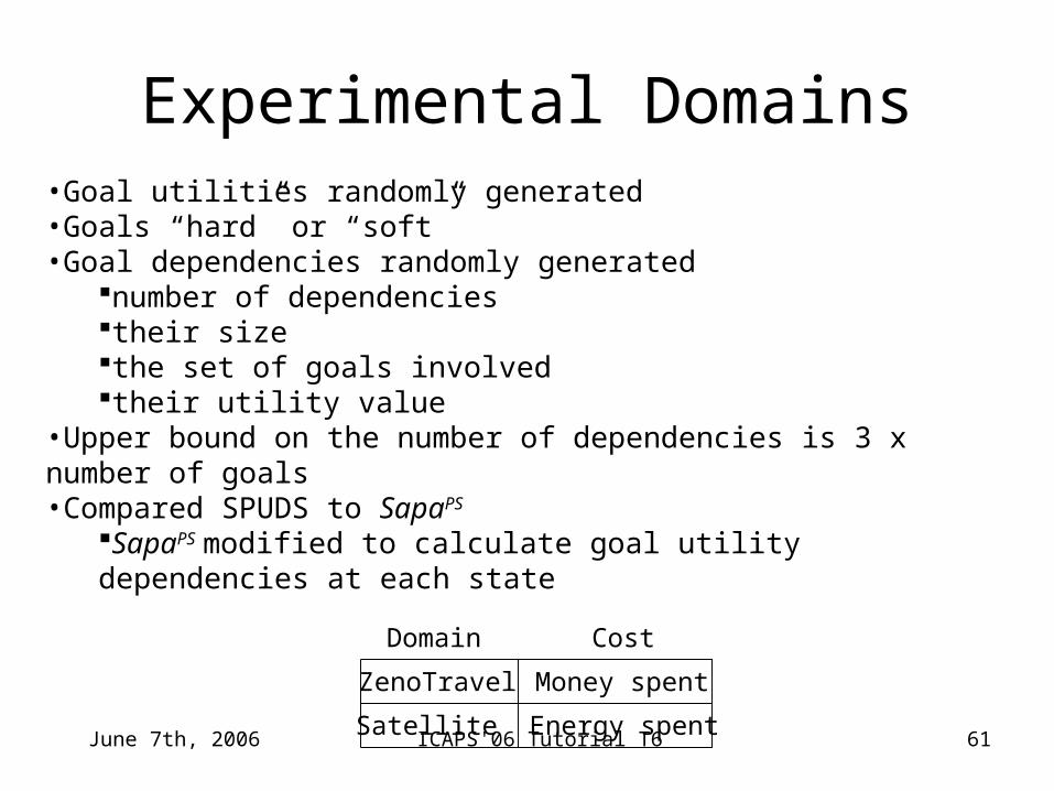
Experimental Domains
ZenoTravel
Satellite
Cost
Money spent
Energy spent
Domain
•Goal utilities randomly generated•Goals “hard” or “soft” •Goal dependencies randomly generated
number of dependenciestheir sizethe set of goals involvedtheir utility value
•Upper bound on the number of dependencies is 3 x number of goals•Compared SPUDS to SapaPS
SapaPS modified to calculate goal utility dependencies at each state
June 7th, 2006 ICAPS'06 Tutorial T6 62
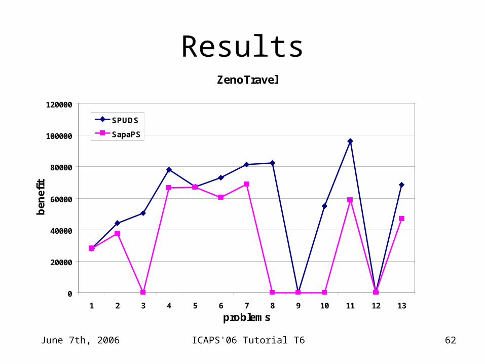
ResultsZenoTravel
0
20000
40000
60000
80000
100000
120000
1 2 3 4 5 6 7 8 9 10 11 12 13
problems
ben
efit
SPUDS
SapaPS
June 7th, 2006 ICAPS'06 Tutorial T6 63
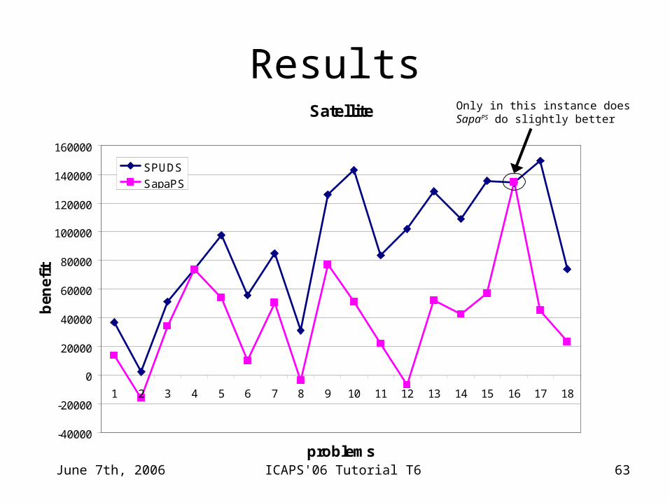
ResultsSatellite
-40000
-20000
0
20000
40000
60000
80000
100000
120000
140000
160000
1 2 3 4 5 6 7 8 9 10 11 12 13 14 15 16 17 18
problems
ben
efit
SPUDS
SapaPS
Only in this instance does SapaPS do slightly better
June 7th, 2006 ICAPS'06 Tutorial T6 64
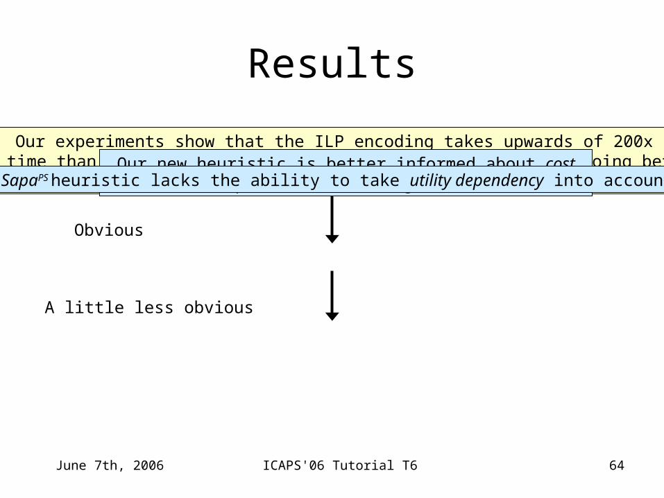
Results
Our experiments show that the ILP encoding takes upwards of 200x more time than then SapaPS procedure per node. Yet it is still doing better.
Why?Our new heuristic is better informed about cost dependencies
between goals. SapaPS heuristic lacks the ability to take utility dependency into account.
Obvious
A little less obvious
June 7th, 2006 ICAPS'06 Tutorial T6 65
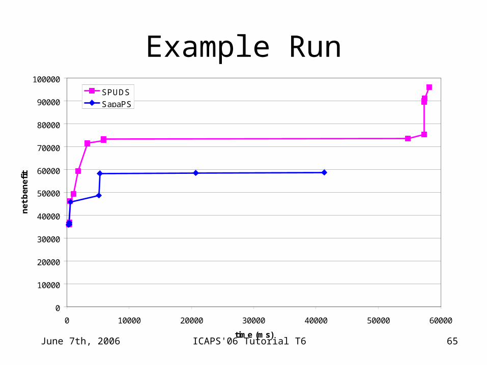
Example Run
0
10000
20000
30000
40000
50000
60000
70000
80000
90000
100000
0 10000 20000 30000 40000 50000 60000
time (ms)
net
ben
efit
SPUDS
SapaPS
June 7th, 2006 ICAPS'06 Tutorial T6 66
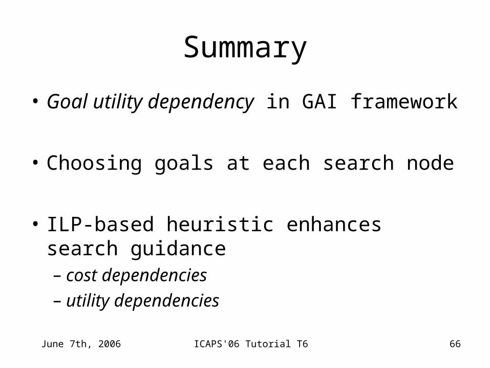
Summary
• Goal utility dependency in GAI framework
• Choosing goals at each search node
• ILP-based heuristic enhances search guidance– cost dependencies– utility dependencies
June 7th, 2006 ICAPS'06 Tutorial T6 67
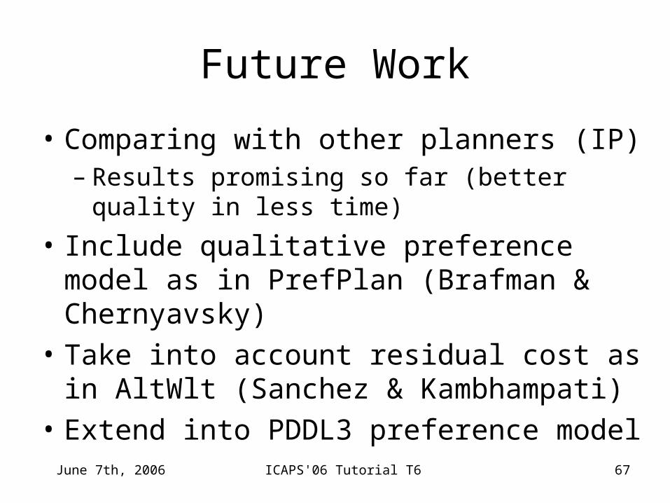
Future Work
• Comparing with other planners (IP)– Results promising so far (better quality in less
time)
• Include qualitative preference model as in PrefPlan (Brafman & Chernyavsky)
• Take into account residual cost as in AltWlt (Sanchez & Kambhampati)
• Extend into PDDL3 preference model
June 7th, 2006 ICAPS'06 Tutorial T6 68
Questions
June 7th, 2006 ICAPS'06 Tutorial T6 69
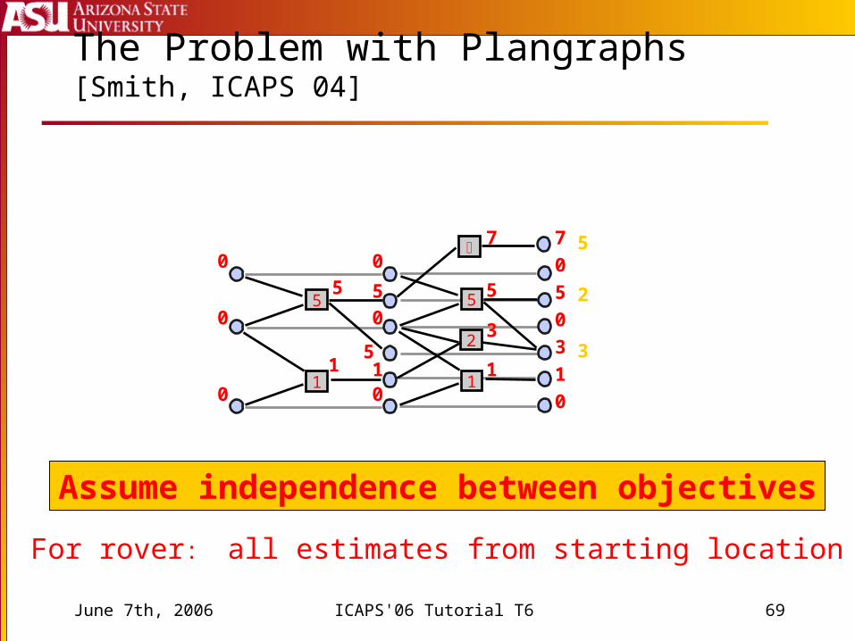
The Problem with Plangraphs [Smith, ICAPS 04]
5
1
5
1
2
0
0
0
0
0
0
5
15
1
5
1
5
7
0
0
0
5
1
3
7
3
5
2
3
Assume independence between objectives
For rover: all estimates from starting location
June 7th, 2006 ICAPS'06 Tutorial T6 70
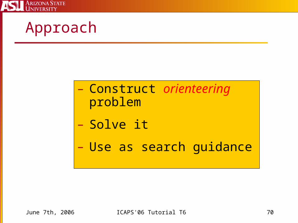
Approach
– Construct orienteering problem
– Solve it
– Use as search guidance
June 7th, 2006 ICAPS'06 Tutorial T6 71
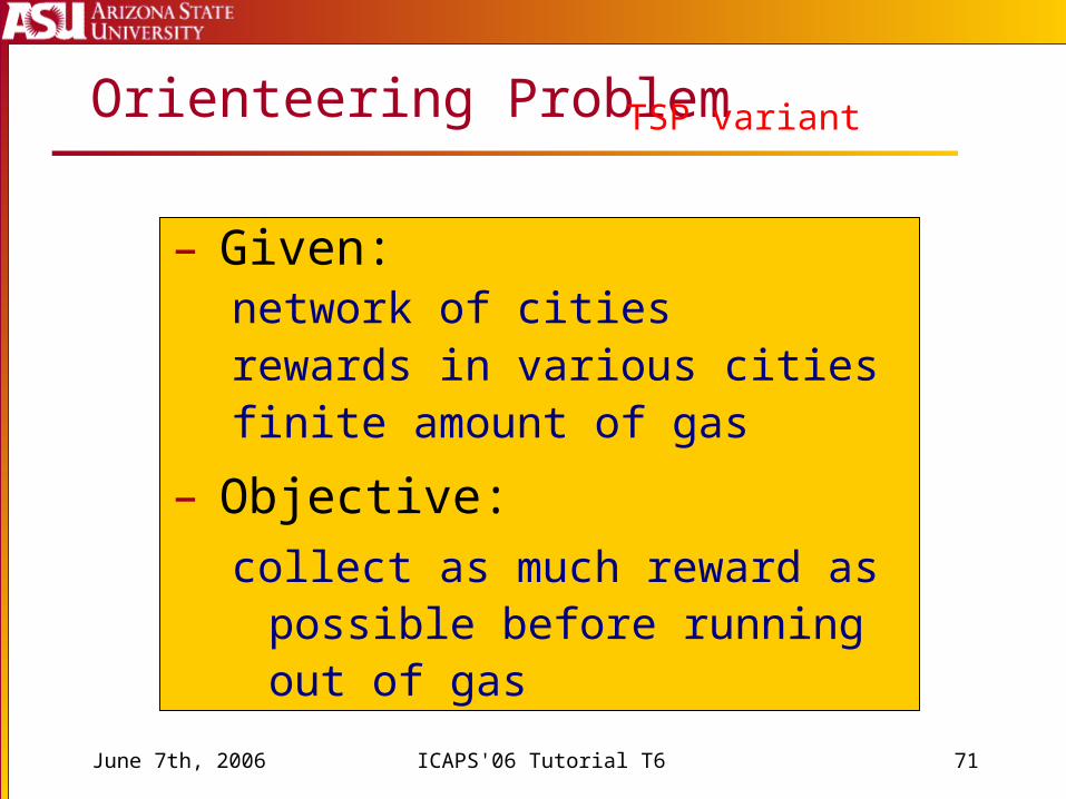
Orienteering Problem
– Given:network of citiesrewards in various citiesfinite amount of gas
– Objective:
collect as much reward as possible before running out of gas
TSP variant
June 7th, 2006 ICAPS'06 Tutorial T6 72
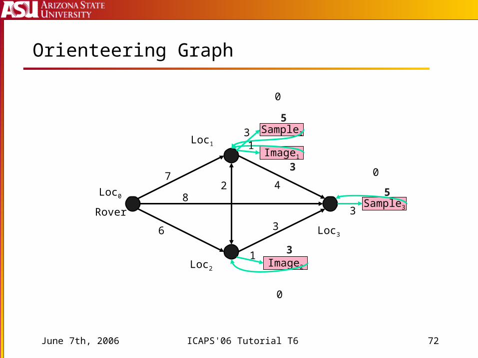
Orienteering Graph
Sample1
Image1
Sample3
Image2
Loc0
Loc1
Loc2
Loc3
Rover
7
6 3
28
4
3
31
0
0
0
1
5
5
3
3
June 7th, 2006 ICAPS'06 Tutorial T6 73
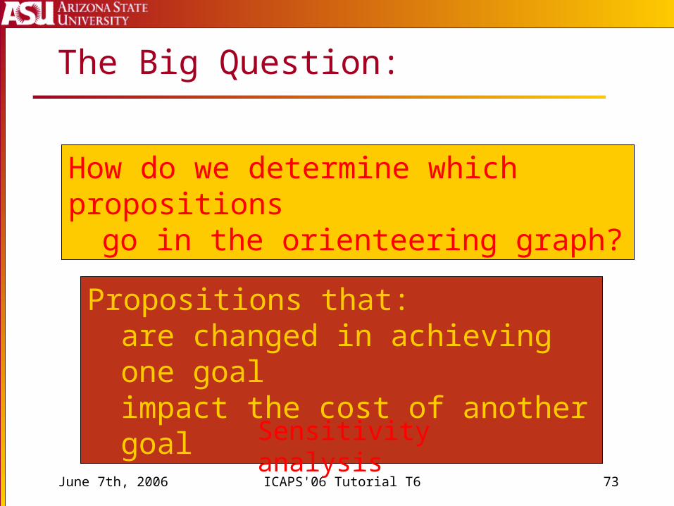
The Big Question:
How do we determine which propositionsgo in the orienteering graph?
Propositions that:are changed in achieving one goalimpact the cost of another goal
Sensitivity analysis
June 7th, 2006 ICAPS'06 Tutorial T6 74
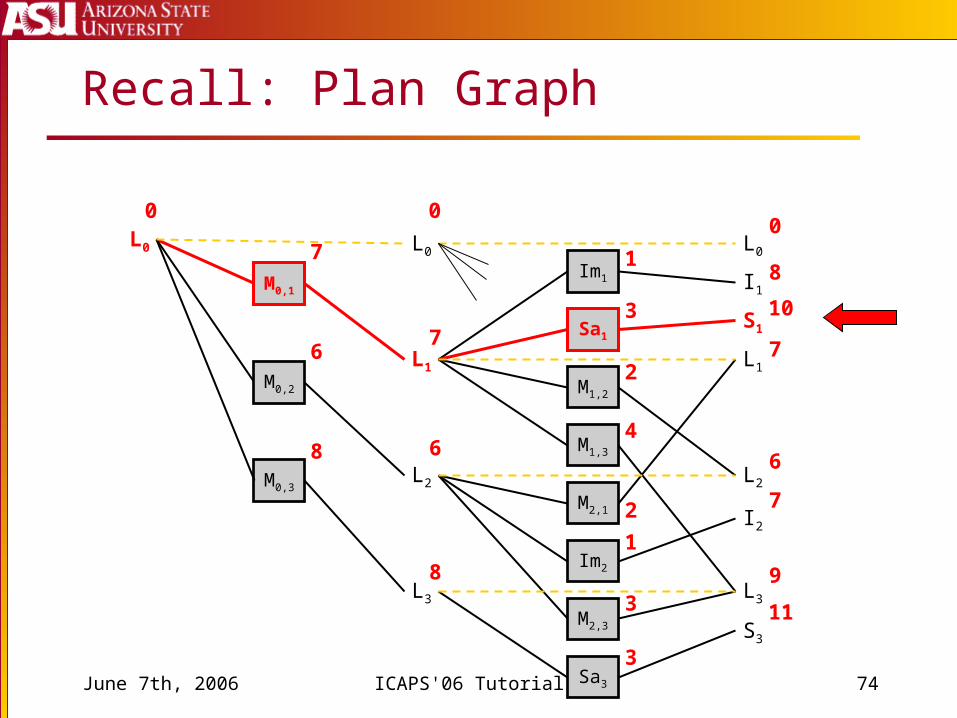
Recall: Plan Graph
0
7L0 L0
L1
L2
L3
M0,1
M0,2
M0,3
Sa1
Im1
M1,2
M1,3
M2,1
Im2
M2,3
Sa3
L0
L1
L2
L3
S1
I1
I2
S3
6
8
7
6
8
0
1
3
2
4
2
1
3
3
0
8
10
7
6
7
9
11
June 7th, 2006 ICAPS'06 Tutorial T6 75
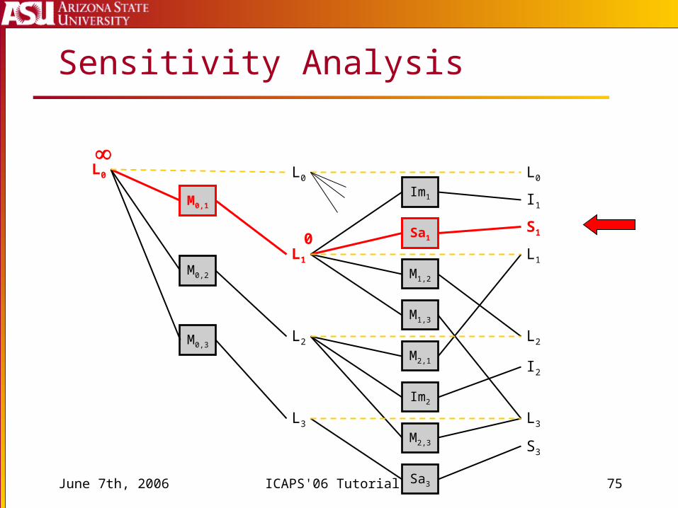
Sensitivity Analysis
L0 L0
L1
L2
L3
M0,1
M0,2
M0,3
Sa1
Im1
M1,2
M1,3
M2,1
Im2
M2,3
Sa3
L0
L1
L2
L3
S1
I1
I2
S3
0
June 7th, 2006 ICAPS'06 Tutorial T6 76
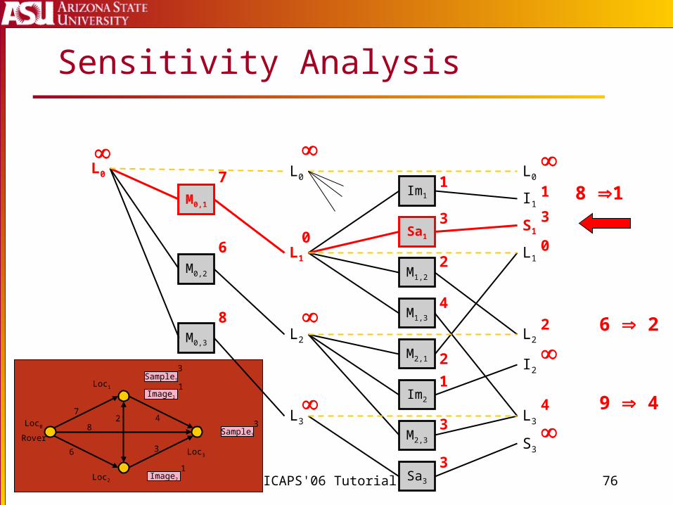
Sample1
Image1
Sample3
Image2
Loc0
Loc1
Loc2
Loc3
Rover
7
6 3
28
43
3
1
1
Sensitivity Analysis
7
L0 L0
L1
L2
L3
M0,1
M0,2
M0,3
Sa1
Im1
M1,2
M1,3
M2,1
Im2
M2,3
Sa3
L0
L1
L2
L3
S1
I1
I2
S3
6
8
0
1
3
2
4
2
1
3
3
1
3
0
2
4
8 1
6 2
9 4
June 7th, 2006 ICAPS'06 Tutorial T6 77
For each goal:Construct a relaxed planFor each net effect of relaxed plan:
Reset costs in PGSet cost of net effect to 0
Set cost of mutex initial conditions to Compute revised cost estimatesIf significantly different,
add net effect to basis set
Basis Set Algorithm
June 7th, 2006 ICAPS'06 Tutorial T6 78
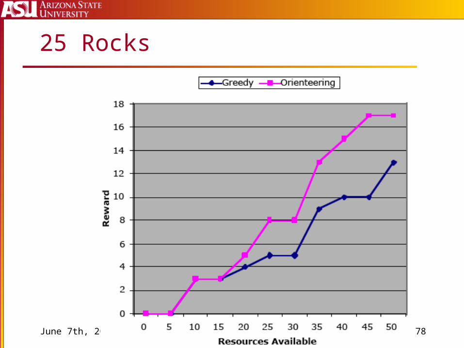
25 Rocks
June 7th, 2006 ICAPS'06 Tutorial T6 79
PSP Conclusions
Goal Set Selection Apriori for Regression Search Anytime for Progression Search Both types of search use greedy goal insertion/removal
to optimize net-benefit of relaxed plans
Orienteering Problem Interactions between goals apparent in OP Use solution to OP as heuristic Planning Graphs help define OP
June 7th, 2006 ICAPS'06 Tutorial T6 80
Planning with Resources
June 7th, 2006 ICAPS'06 Tutorial T6 81
Planning with Resources
Propagating Resource Intervals Relaxed Plans
Handling resource subgoals
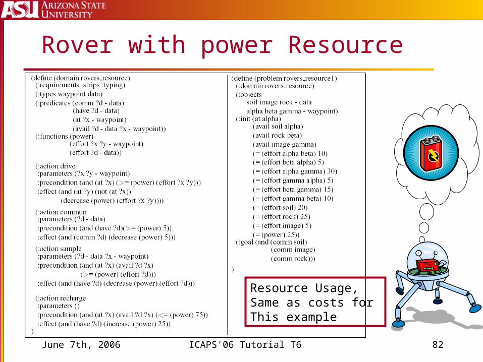
June 7th, 2006 ICAPS'06 Tutorial T6 82
Rover with power Resource
Resource Usage,Same as costs for This example
June 7th, 2006 ICAPS'06 Tutorial T6 83
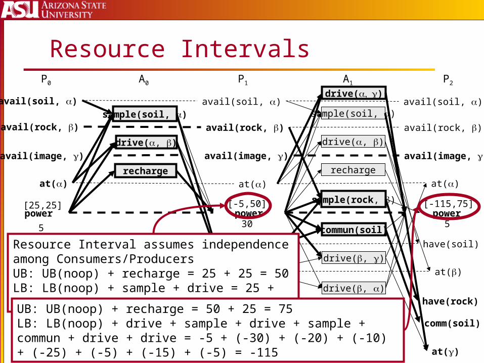
Resource Intervals
at()
avail(soil, )
avail(rock, )
avail(image, )
sample(soil, )
drive(, )
at()
avail(soil, )
avail(rock, )
avail(image, )
at()
have(soil)
sample(soil, )
drive(, )
recharge
at()
avail(soil, )
avail(rock, )
avail(image, )
at()
at()
have(soil)
drive(, )
drive(, )
commun(soil)
sample(rock, )
comm(soil)
have(rock)
power [-5,50]
recharge
power [25,25]
drive()
power [-115,75]
5305
A1A0 P1P0 P2
Resource Interval assumes independenceamong Consumers/ProducersUB: UB(noop) + recharge = 25 + 25 = 50LB: LB(noop) + sample + drive = 25 + (-20) + (-10) = -5
UB: UB(noop) + recharge = 50 + 25 = 75LB: LB(noop) + drive + sample + drive + sample + commun + drive + drive = -5 + (-30) + (-20) + (-10) + (-25) + (-5) + (-15) + (-5) = -115
June 7th, 2006 ICAPS'06 Tutorial T6 84
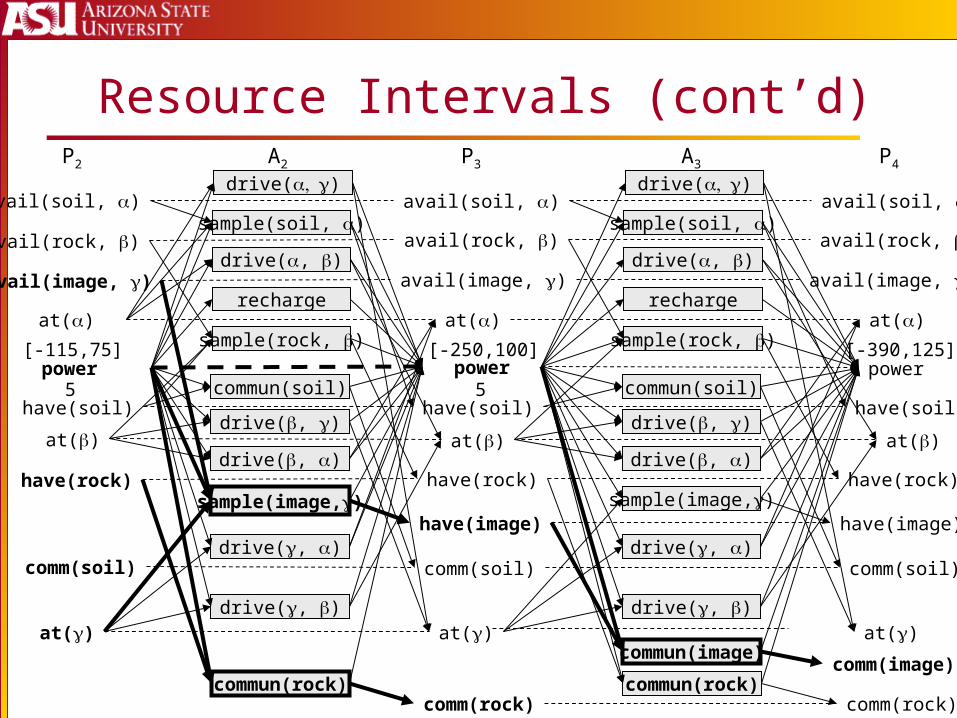
Resource Intervals (cont’d)
at()
avail(soil, )
avail(rock, )
avail(image, )
at()
at()
have(soil)
comm(soil)
have(rock)
commun(image)
commun(rock)comm(image)
comm(rock)
at()
at()
at()
have(soil)drive(, )
drive(, )
drive(, )
commun(soil)
sample(image,)
drive(, )
have(image)
comm(soil)
have(rock)
sample(soil, )
drive(, )
recharge
avail(soil, )
avail(rock, )
avail(image, )
drive()
sample(rock, )
commun(rock)comm(rock)
at()
at()
at()
have(soil)drive(, )
drive(, )
drive(, )
commun(soil)
sample(image,)
drive(, )
have(image)
comm(soil)
have(rock)
sample(soil, )
drive(, )
recharge
avail(soil, )
avail(rock, )
avail(image, )
power [-115,75]
power [-250,100]
power[-390,125]
drive()
sample(rock, )
55
A2P2 P3 A3 P4
June 7th, 2006 ICAPS'06 Tutorial T6 85
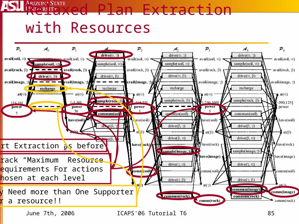
Relaxed Plan Extraction with Resources
Start Extraction as before
Track “Maximum” Resource Requirements For actions chosen at each level
May Need more than One SupporterFor a resource!!
June 7th, 2006 ICAPS'06 Tutorial T6 86
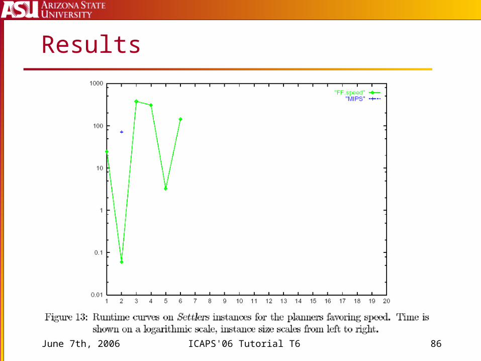
Results
June 7th, 2006 ICAPS'06 Tutorial T6 87
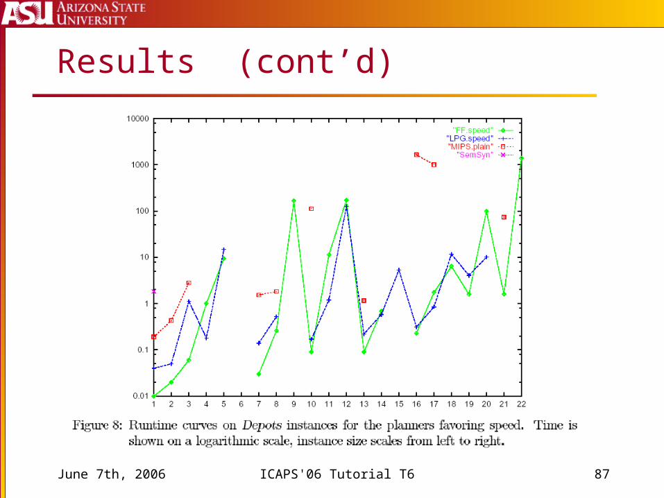
Results (cont’d)
June 7th, 2006 ICAPS'06 Tutorial T6 88
Planning With Resources Conclusion
Resource Intervals allow us to be optimistic about reachable values Upper/Lower bounds can get large
Relaxed Plans may require multiple supporters for subgoals
Negative Interactions are much harder to capture
June 7th, 2006 ICAPS'06 Tutorial T6 89
Temporal Planning
June 7th, 2006 ICAPS'06 Tutorial T6 90
Temporal Planning
Temporal Planning Graph From Levels to Time Points Delayed Effects
Estimating Makespan Relaxed Plan Extraction
June 7th, 2006 ICAPS'06 Tutorial T6 91
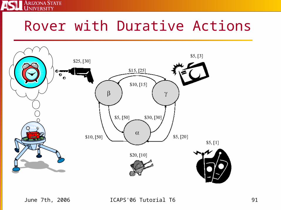
Rover with Durative Actions
June 7th, 2006 ICAPS'06 Tutorial T6 92
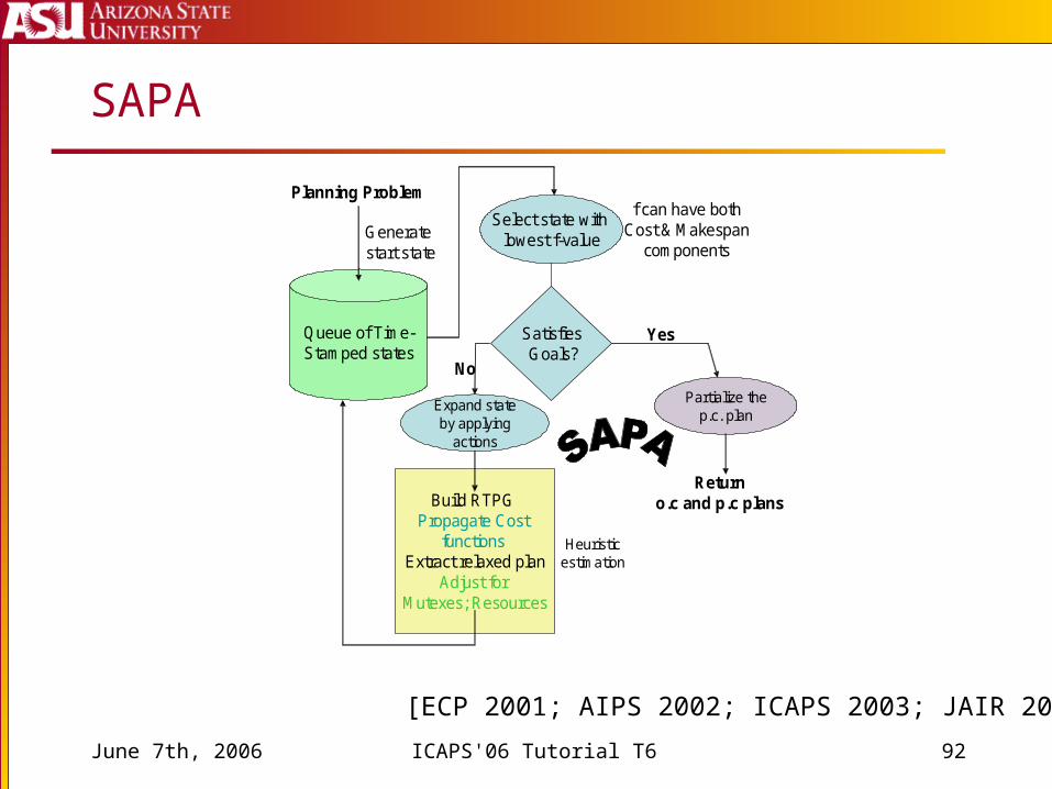
SAPA
Build RTPG Propagate Cost
functionsExtract relaxed plan
Adjust for Mutexes; Resources
Planning Problem
Generate start state
No
Partialize thep.c. plan
Returno.c and p.c plans
Expand state by applying
actions
Heuristicestimation
Select state with lowest f-value
SatisfiesGoals?
Queue of Time-Stamped states
Yes
f can have bothCost & Makespan
components
[ECP 2001; AIPS 2002; ICAPS 2003; JAIR 2003]
June 7th, 2006 ICAPS'06 Tutorial T6 93
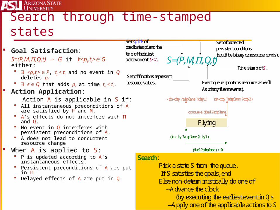
Search through time-stamped states
S=(P,M,,Q,t)
Set <pi,ti> of predicates pi and thetime of their last achievement ti < t.
Set <pi,ti> of predicates pi and thetime of their last achievement ti < t.
Set of functions represent resource values.Set of functions represent resource values.
Set of protectedpersistent conditions(could be binary or resource conds).
Set of protectedpersistent conditions(could be binary or resource conds).
Event queue (contains resource as wellAs binary fluent events).Event queue (contains resource as wellAs binary fluent events).
Time stamp of S.Time stamp of S.
Flying
(in-city ?airplane ?city1)
(fuel ?airplane) > 0
(in-city ?airplane ?city1) (in-city ?airplane ?city2)
consume (fuel ?airplane)
Flying
(in-city ?airplane ?city1)
(fuel ?airplane) > 0
(in-city ?airplane ?city1) (in-city ?airplane ?city2)
consume (fuel ?airplane)
Goal Satisfaction: S=(P,M,,Q,t) G if <pi,ti> G either:
<pi,tj> P, tj < ti and no event in Q deletes pi.
e Q that adds pi at time te < ti. Action Application: Action A is applicable in S if:
All instantaneous preconditions of A are satisfied by P and M.
A’s effects do not interfere with and Q. No event in Q interferes with persistent
preconditions of A. A does not lead to concurrent resource
change When A is applied to S:
P is updated according to A’s instantaneous effects.
Persistent preconditions of A are put in Delayed effects of A are put in Q.
Search: Pick a state S from the queue. If S satisfies the goals, endElse non-deterministically do one of
--Advance the clock (by executing the earliest event in Qs
--Apply one of the applicable actions to S
June 7th, 2006 ICAPS'06 Tutorial T6 94
sample(rock, )
1000 5010 20 30 40 60 70 80 90
drive(, )
drive(, )
commun(soil)
sample(soil, )
commun(rock)
drive(, )
drive(, )
drive(, )
drive(, )
commun(image)
sample(image, )
have(soil)
comm(soil)
at() at()
have(image)
comm(image)
have(rock)
comm(rock)
avail(soil,)
avail(rock,)
avail(image,)
at()
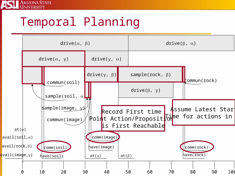
Temporal Planning
Record First time Point Action/Proposition
is First Reachable
Assume Latest StartTime for actions in RP
June 7th, 2006 ICAPS'06 Tutorial T6 95
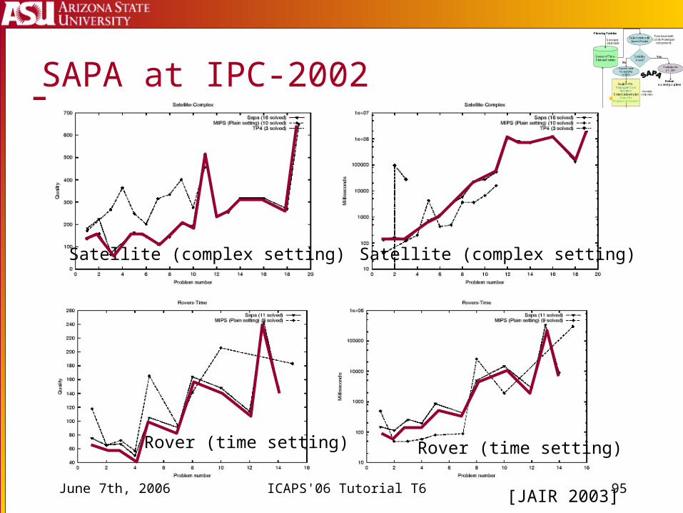
SAPA at IPC-2002
Rover (time setting) Rover (time setting)
Satellite (complex setting) Satellite (complex setting)
Build RTPG Propagate Cost
functionsExtract relaxed plan
Adjust for Mutexes; Resources
Planning Problem
Generate start state
No
Partialize thep.c. plan
Returno.c and p.c plans
Expand state by applying
actions
Heuristicestimation
Select state with lowest f-value
SatisfiesGoals?
Queue of Time-Stamped states
Yes
f can have bothCost & Makespan
components
[JAIR 2003]
June 7th, 2006 ICAPS'06 Tutorial T6 96
Temporal Planning Conclusion
Levels become Time Points Makespan and plan length/cost are different
objectives Set-Level heuristic measures makespan Relaxed Plans measure makespan and plan
cost
June 7th, 2006 ICAPS'06 Tutorial T6 97
Non-Deterministic Planning
June 7th, 2006 ICAPS'06 Tutorial T6 98
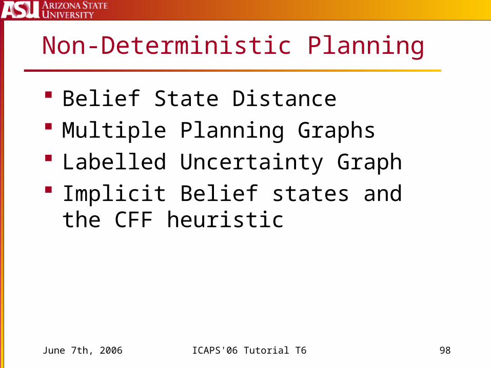
Non-Deterministic Planning
Belief State Distance Multiple Planning Graphs Labelled Uncertainty Graph Implicit Belief states and the CFF heuristic
June 7th, 2006 ICAPS'06 Tutorial T6 99
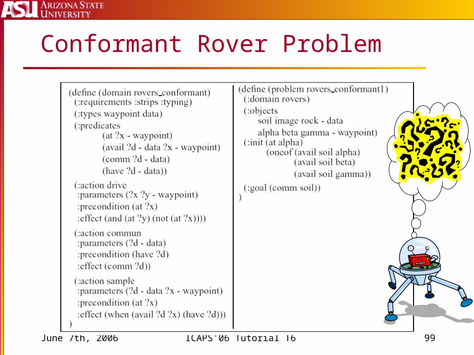
Conformant Rover Problem
June 7th, 2006 ICAPS'06 Tutorial T6 100
Search in Belief State Space
at()
avail(soil, )
at()
avail(soil, )
at()
avail(soil, )
at()avail(soil, )
at()
avail(soil, )
at()
avail(soil, )
at()
avail(soil, )
at()
avail(soil, )
at()
avail(soil, )
sample(soil, )
drive(, )
have(soil)
drive(, )
at()avail(soil, )
at()
avail(soil, )
at()
avail(soil, )
drive(, )have(soil)
drive(, )
at()avail(soil, )
at()avail(soil, )
at()
avail(soil, )
sample(soil, )
drive(b, )
have(soil)
sample(soil, )
at()avail(soil, )
have(soil)
at()avail(soil, )
have(soil)
at()
avail(soil, )
June 7th, 2006 ICAPS'06 Tutorial T6 101
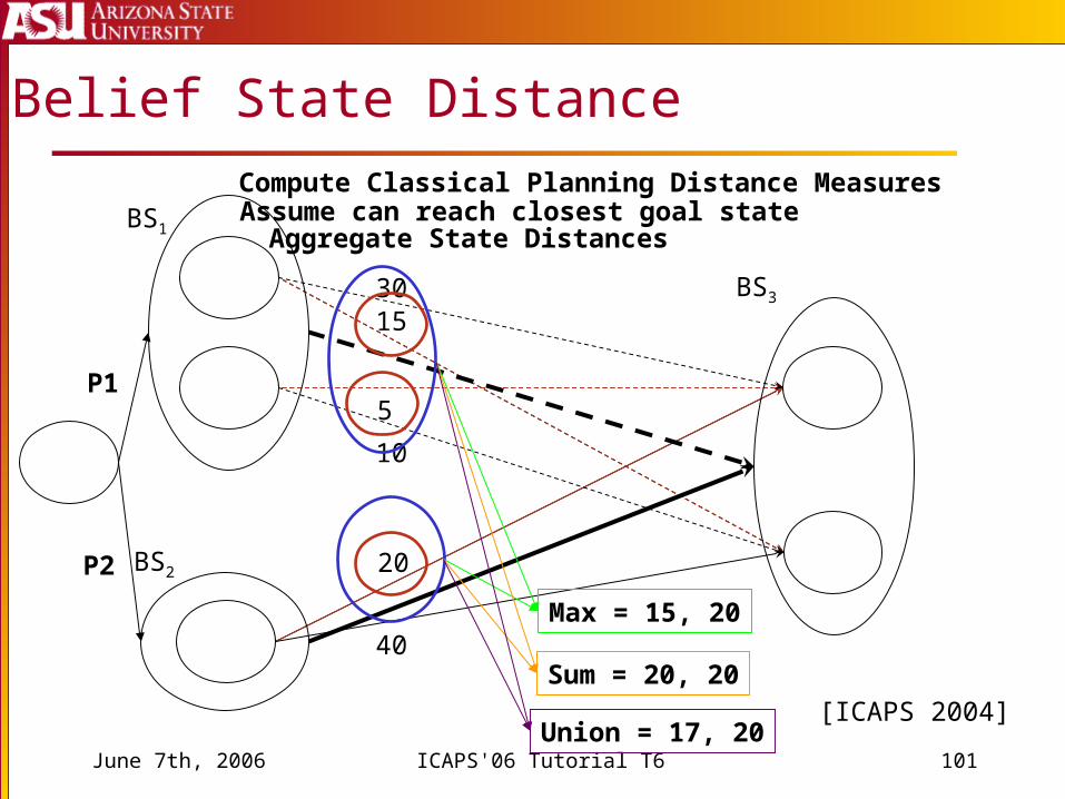
Belief State Distance
BS3
BS1
BS2 20
40
3015
5
10
Max = 15, 20
Sum = 20, 20
Union = 17, 20[ICAPS 2004]
P2
P1
Compute Classical Planning Distance MeasuresAssume can reach closest goal stateAggregate State Distances
June 7th, 2006 ICAPS'06 Tutorial T6 102
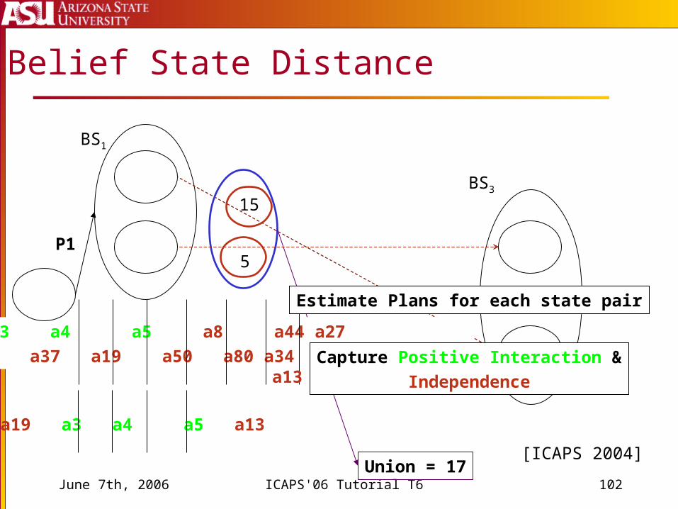
Belief State Distance
BS3
BS1
15
5
Union = 17
a1 a3 a4 a5 a8 a44 a27
a14 a22 a37 a19 a50 a80 a34 a11
a19 a3 a4 a5 a13
a19 a13
P1
Capture Positive Interaction &
Independence
Estimate Plans for each state pair
[ICAPS 2004]
June 7th, 2006 ICAPS'06 Tutorial T6 103
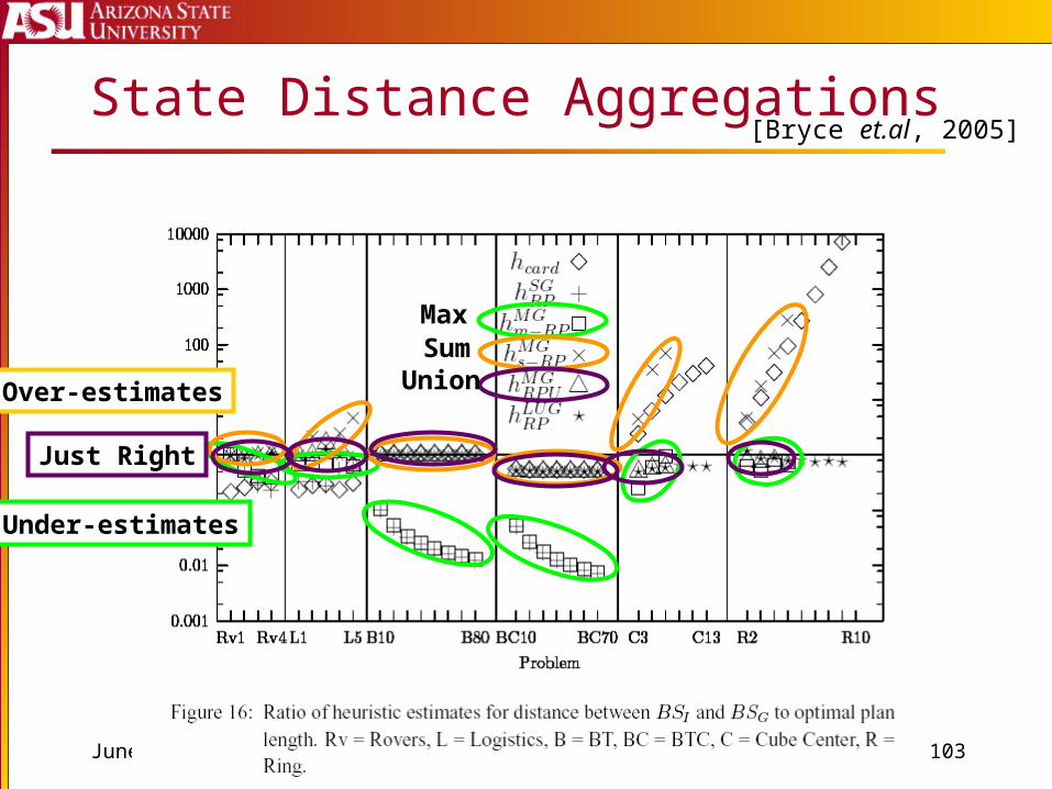
State Distance Aggregations
MaxSum
Union
Under-estimates
Over-estimates
Just Right
[Bryce et.al, 2005]
June 7th, 2006 ICAPS'06 Tutorial T6 104
at()
sample(soil, )
drive(, )
drive(, )
avail(soil, )
at()
avail(soil, )
at()
at()
have(soil)
at()drive(, )
drive(, )
avail(soil, )
at()
avail(soil, )
at()
at()
drive(, )
drive(, )at()
avail(soil, )
at()
at()sample(soil, )
have(soil)
drive(, )drive(, )
drive(, )drive(, )
at()drive(, )
drive(, )
avail(soil, )
at()
avail(soil, )
at()
at()
drive(, )
drive(, )at()
avail(soil, )
at()
at()sample(soil, )
have(soil)
drive(, )drive(, )drive(, )drive(, )
drive(, )
drive(, )at()
avail(soil, )
at()
at()sample(soil, )
have(soil)
drive(, )drive(, )
drive(, )drive(, )
commun(soil) comm(soil)
commun(soil) comm(soil)
sample(soil, )
drive(, )
drive(, ) at()
avail(soil, )
at()
at()
have(soil)
drive(, )
drive(, )at()
avail(soil, )
at()
at()sample(soil, )
have(soil)
drive(, )drive(, )
drive(, )drive(, )
commun(soil) comm(soil)
A1A0 A2P1P0 P2 P3
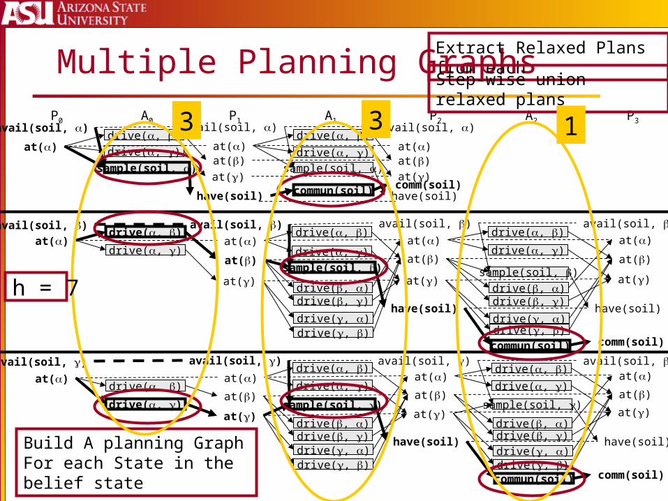
Multiple Planning Graphs
Build A planning Graph For each State in the belief state
Extract Relaxed Plans from each
Step-wise union relaxed plans
133
h = 7
June 7th, 2006 ICAPS'06 Tutorial T6 105
sample(soil, )
avail(soil, ) avail(soil, )
have(soil)
at()drive(, )
drive(, )
avail(soil, )
at()
avail(soil, )
at()
at()
drive(, )
drive(, )
at()
avail(soil, )
at()
at()
sample(soil, )
have(soil)
drive(, )
drive(, )
drive(, )
drive(, )
avail(soil, ) avail(soil, ) avail(soil, )
sample(soil, )
drive(, )
drive(, )
at()
avail(soil, )
at()
at()
sample(soil, )
have(soil)
drive(, )
drive(, )
drive(, )
drive(, )
commun(soil)
comm(soil)
commun(soil)
comm(soil)
sample(soil, )
avail(soil, )
avail(soil, )
sample(soil, )
sample(soil, )
avail(soil, )
A1A0 A2P1P0 P2 P3
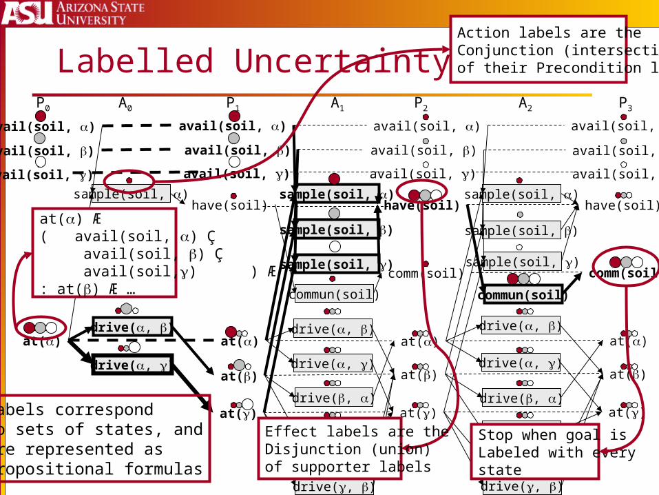
Labelled Uncertainty Graph
Labels correspondTo sets of states, andAre represented as Propositional formulas
at() Æ ( avail(soil, ) Ç avail(soil, ) Ç avail(soil,) ) Æ: at() Æ …
Action labels are the Conjunction (intersection)of their Precondition labels
Effect labels are the Disjunction (union) of supporter labels
Stop when goal is Labeled with every state
June 7th, 2006 ICAPS'06 Tutorial T6 106
sample(soil, )
avail(soil, ) avail(soil, )
have(soil)
at()drive(, )
drive(, )
avail(soil, )
at()
avail(soil, )
at()
at()
drive(, )
drive(, )
at()
avail(soil, )
at()
at()
sample(soil, )
have(soil)
drive(, )
drive(, )
drive(, )
drive(, )
avail(soil, ) avail(soil, ) avail(soil, )
sample(soil, )
drive(, )
drive(, )
at()
avail(soil, )
at()
at()
sample(soil, )
have(soil)
drive(, )
drive(, )
drive(, )
drive(, )
commun(soil)
comm(soil)
commun(soil)
comm(soil)
sample(soil, )
avail(soil, )
avail(soil, )
sample(soil, )
sample(soil, )
avail(soil, )
A1A0 A2P1P0 P2 P3
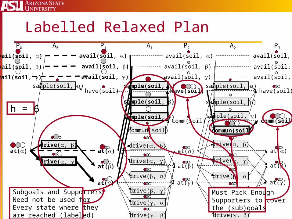
Labelled Relaxed Plan
Must Pick Enough Supporters to coverthe (sub)goals
Subgoals and SupportersNeed not be used for Every state where they are reached (labeled)
h = 6
June 7th, 2006 ICAPS'06 Tutorial T6 107
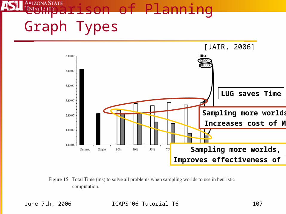
Comparison of Planning Graph Types[JAIR, 2006]
LUG saves Time
Sampling more worlds,
Increases cost of MG
Sampling more worlds,
Improves effectiveness of LUG
June 7th, 2006 ICAPS'06 Tutorial T6 108
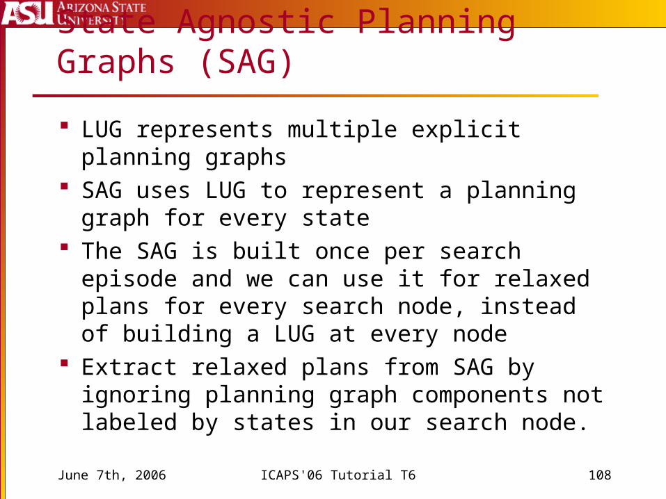
State Agnostic Planning Graphs (SAG)
LUG represents multiple explicit planning graphs SAG uses LUG to represent a planning graph for
every state The SAG is built once per search episode and we
can use it for relaxed plans for every search node, instead of building a LUG at every node
Extract relaxed plans from SAG by ignoring planning graph components not labeled by states in our search node.
June 7th, 2006 ICAPS'06 Tutorial T6 109
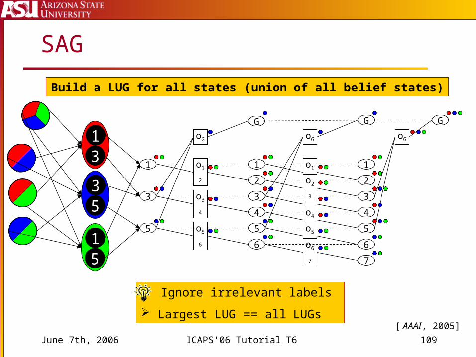
SAG
13
15
1
3
4
5
1
3
5
o12
o34
o56
2
1
3
4
5
o12
o34
o23
o45
o56
2
6 6
7o67
oG
G G G
oG oG
35
Ignore irrelevant labels
Largest LUG == all LUGs[ AAAI, 2005]
Build a LUG for all states (union of all belief states)
June 7th, 2006 ICAPS'06 Tutorial T6 110
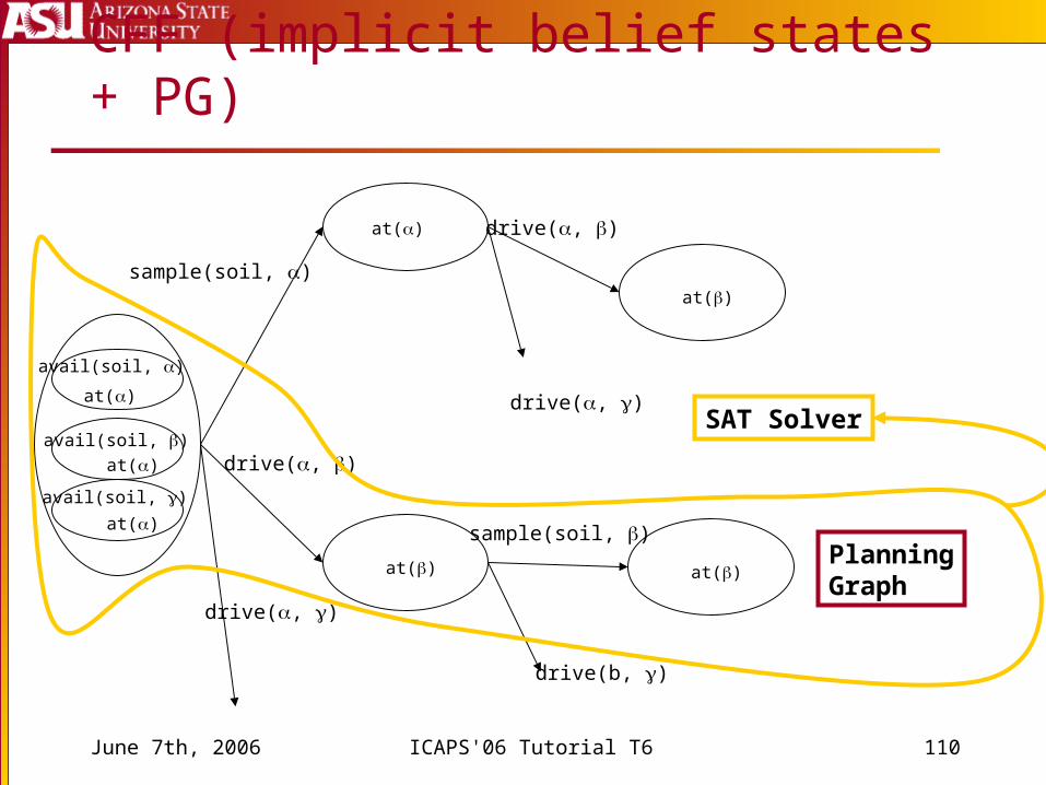
CFF (implicit belief states + PG)
at()
avail(soil, )
at()
avail(soil, )
at()
avail(soil, )
at()
sample(soil, )
drive(, )
drive(, )
drive(, )
drive(, )
sample(soil, )
drive(b, )
at()
at()
at()PlanningGraph
SAT Solver

June 7th, 2006 ICAPS'06 Tutorial T6 111
Belief Space Problems Classical Problems
Conformant ConditionalMore Results at the IPC!!!
June 7th, 2006 ICAPS'06 Tutorial T6 112
Conditional Planning
Actions have Observations Observations branch the plan because:
Plan Cost is reduced by performing less “just in case” actions – each branch performs relevant actions
Sometimes actions conflict and observing determines which to execute (e.g., medical treatments)
We are ignoring negative interactions We are only forced to use observations to remove
negative interactions Ignore the observations and use the conformant relaxed
plan Suitable because the aggregate search effort over all plan
branches is related to the conformant relaxed plan cost
June 7th, 2006 ICAPS'06 Tutorial T6 113
Non-Deterministic Planning Conclusions
Measure positive interaction and independence between states co-transitioning to the goal via overlap Labeled planning graphs and CFF SAT
encoding efficiently measure conformant plan distance
Conformant planning heuristics work for conditional planning without modification
June 7th, 2006 ICAPS'06 Tutorial T6 114
Stochastic Planning
June 7th, 2006 ICAPS'06 Tutorial T6 115
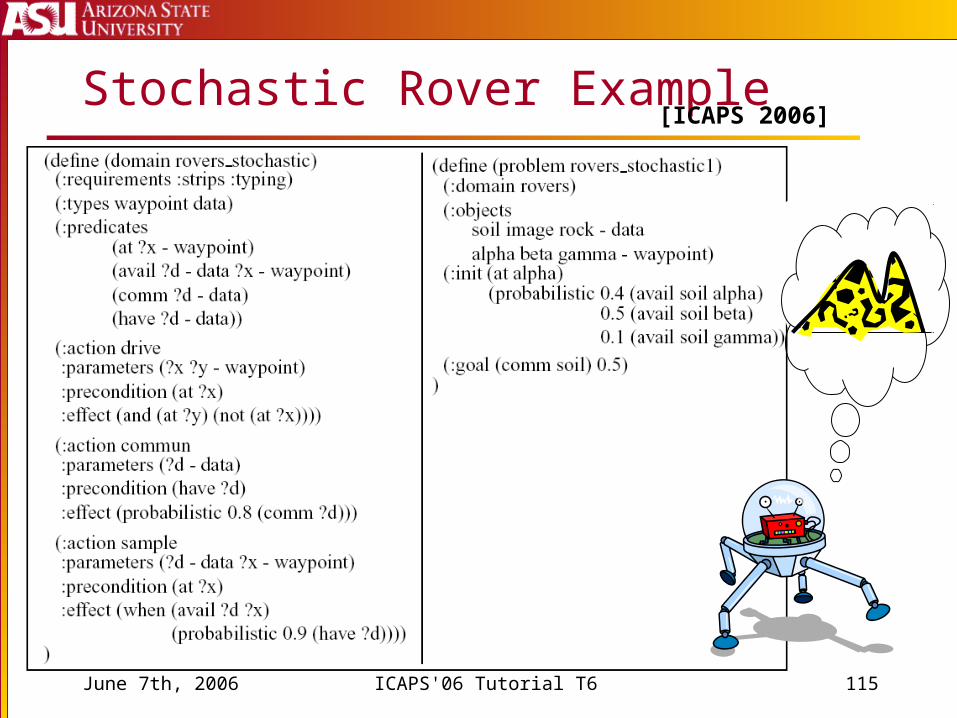
Stochastic Rover Example[ICAPS 2006]
June 7th, 2006 ICAPS'06 Tutorial T6 116
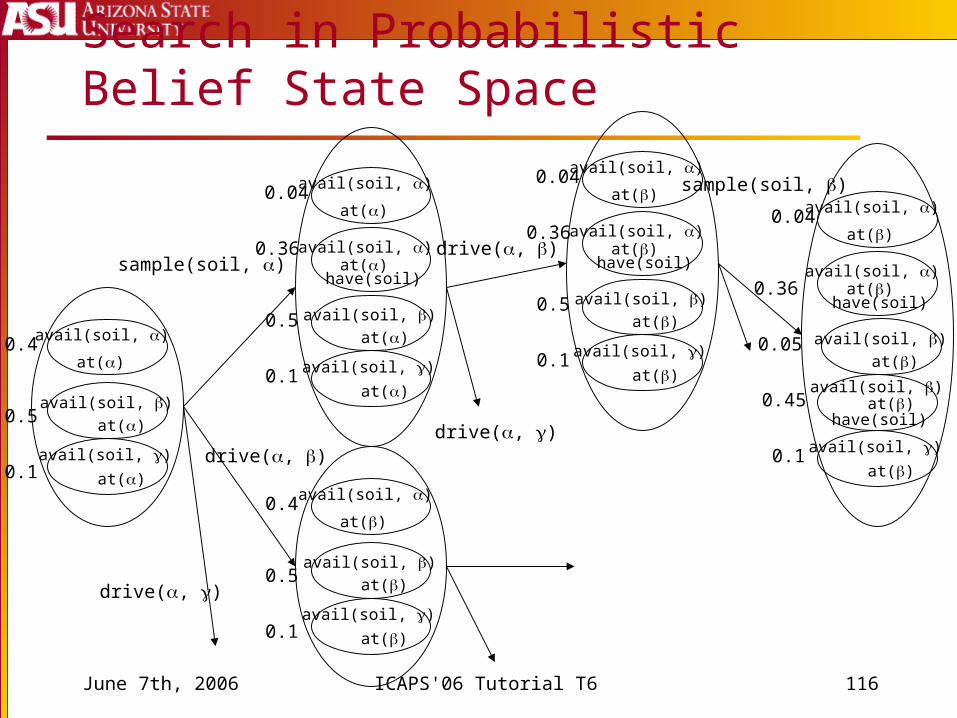
Search in Probabilistic Belief State Space
at()
avail(soil, )
at()
avail(soil, )
at()
avail(soil, )
at()avail(soil, )
at()
avail(soil, )
at()
avail(soil, )
at()
avail(soil, )
at()
avail(soil, )
at()
avail(soil, )
sample(soil, )
drive(, )
have(soil)
drive(, )
drive(, )
drive(, )
sample(soil, )
0.4
0.5
0.1
at()
avail(soil, )
0.36
0.5
0.1
0.4
0.5
0.1
0.04
at()avail(soil, )
at()
avail(soil, )
at()
avail(soil, )
have(soil)
at()
avail(soil, )
0.36
0.5
0.1
0.04
at()avail(soil, )
at()avail(soil, )
at()
avail(soil, )
have(soil)
at()
avail(soil, )
0.45
0.1
0.04
0.36
at()
avail(soil, )
have(soil)
0.05
June 7th, 2006 ICAPS'06 Tutorial T6 117
Handling Uncertain Actions
Extending LUG to handle uncertain actions requires label extension that captures: State uncertainty (as before) Action outcome uncertainty
Problem: Each action at each level may have a different outcome. The number of uncertain events grows over time – meaning the number of joint outcomes of events grows exponentially with time
Solution: Not all outcomes are important. Sample some of them – keep number of joint outcomes constant.
[ICAPS 2006]
June 7th, 2006 ICAPS'06 Tutorial T6 118
Monte Carlo LUG (McLUG)
Use Sequential Monte Carlo in the Relaxed Planning Space Build several deterministic planning graphs by
sampling states and action outcomes Represent set of planning graphs using LUG
techniques Labels are sets of particles Sample which Action outcomes get labeled with
particles Bias relaxed plan by picking actions labeled with
most particles to prefer more probable support
[ICAPS 2006]
June 7th, 2006 ICAPS'06 Tutorial T6 119
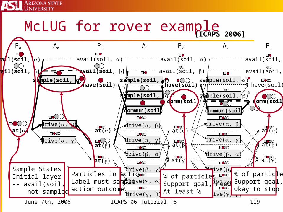
McLUG for rover example
sample(soil, )
avail(soil, ) avail(soil, )
have(soil)
at()drive(, )
drive(, )
avail(soil, )
at()
avail(soil, )
at()
at()
drive(, )
drive(, )
at()
avail(soil, )
at()
at()
sample(soil, )
have(soil)
drive(, )
drive(, )
drive(, )
drive(, )
drive(, )
drive(, )
at()
avail(soil, )
at()
at()
sample(soil, )
have(soil)
drive(, )
drive(, )
drive(, )
drive(, )
commun(soil)
comm(soil)
commun(soil)
comm(soil)
sample(soil, )
avail(soil, )
sample(soil, )
avail(soil, )
A1A0 A2P1P0 P2 P3
Sample States for Initial layer-- avail(soil, ) not sampled
Particles in action Label must sample action outcome
¼ of particles Support goal, needAt least ½
¾ of particles Support goal, Okay to stop
[ICAPS 2006]
June 7th, 2006 ICAPS'06 Tutorial T6 120
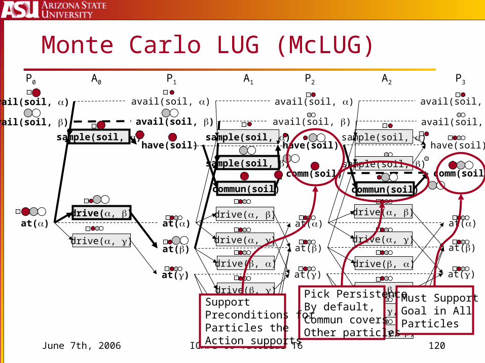
Monte Carlo LUG (McLUG)
sample(soil, )
avail(soil, ) avail(soil, )
have(soil)
at()drive(, )
drive(, )
avail(soil, )
at()
avail(soil, )
at()
at()
drive(, )
drive(, )
at()
avail(soil, )
at()
at()
sample(soil, )
have(soil)
drive(, )
drive(, )
drive(, )
drive(, )
drive(, )
drive(, )
at()
avail(soil, )
at()
at()
sample(soil, )
have(soil)
drive(, )
drive(, )
drive(, )
drive(, )
commun(soil)
comm(soil)
commun(soil)
comm(soil)
sample(soil, )
avail(soil, )
sample(soil, )
avail(soil, )
A1A0 A2P1P0 P2 P3
Must SupportGoal in All Particles
Pick PersistenceBy default,Commun coversOther particles
Support Preconditions forParticles the Action supports
June 7th, 2006 ICAPS'06 Tutorial T6 121
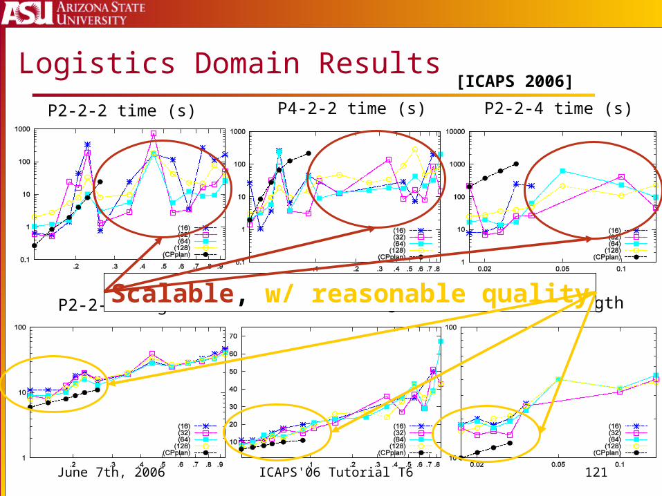
Logistics Domain Results
P2-2-2 time (s) P4-2-2 time (s) P2-2-4 time (s)
P2-2-2 length P4-2-2 length P2-2-4 length
[ICAPS 2006]
Scalable, w/ reasonable quality
June 7th, 2006 ICAPS'06 Tutorial T6 122
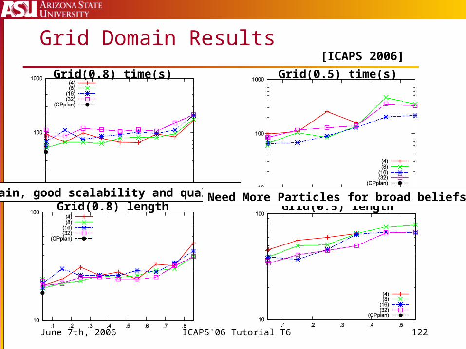
Grid Domain Results
Grid(0.8) time(s)
Grid(0.8) length
Grid(0.5) time(s)
Grid(0.5) lengthAgain, good scalability and quality! Need More Particles for broad beliefs
[ICAPS 2006]
June 7th, 2006 ICAPS'06 Tutorial T6 123
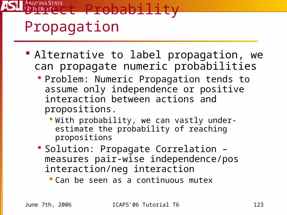
Direct Probability Propagation
Alternative to label propagation, we can propagate numeric probabilities Problem: Numeric Propagation tends to assume
only independence or positive interaction between actions and propositions. With probability, we can vastly under-estimate the
probability of reaching propositions Solution: Propagate Correlation – measures
pair-wise independence/pos interaction/neg interaction Can be seen as a continuous mutex
June 7th, 2006 ICAPS'06 Tutorial T6 124
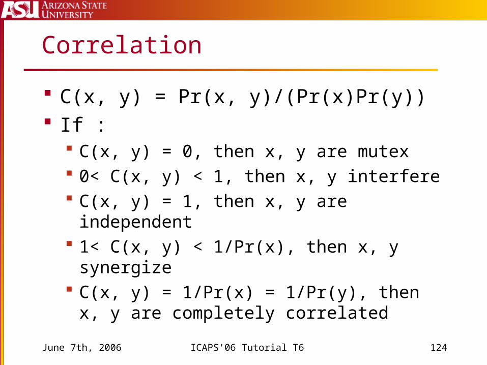
Correlation
C(x, y) = Pr(x, y)/(Pr(x)Pr(y)) If :
C(x, y) = 0, then x, y are mutex 0< C(x, y) < 1, then x, y interfere C(x, y) = 1, then x, y are independent 1< C(x, y) < 1/Pr(x), then x, y synergize C(x, y) = 1/Pr(x) = 1/Pr(y), then x, y are
completely correlated
June 7th, 2006 ICAPS'06 Tutorial T6 125
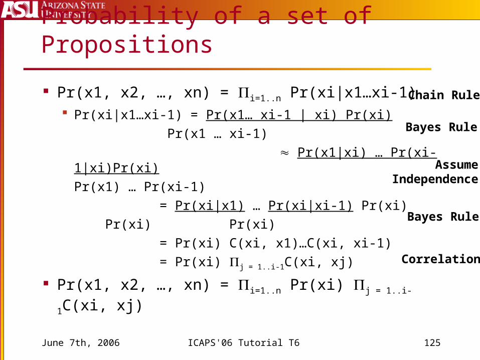
Probability of a set of Propositions
Pr(x1, x2, …, xn) = i=1..n Pr(xi|x1…xi-1) Pr(xi|x1…xi-1) = Pr(x1… xi-1 | xi) Pr(xi)
Pr(x1 … xi-1)
Pr(x1|xi) … Pr(xi-1|xi)Pr(xi)
Pr(x1) … Pr(xi-1)
= Pr(xi|x1) … Pr(xi|xi-1) Pr(xi)
Pr(xi) Pr(xi)
= Pr(xi) C(xi, x1)…C(xi, xi-1)
= Pr(xi) j = 1..i-1C(xi, xj)
Pr(x1, x2, …, xn) = i=1..n Pr(xi) j = 1..i-1C(xi, xj)
Chain Rule
Bayes Rule
AssumeIndependence
Bayes Rule
Correlation
June 7th, 2006 ICAPS'06 Tutorial T6 126
Probability Propagation
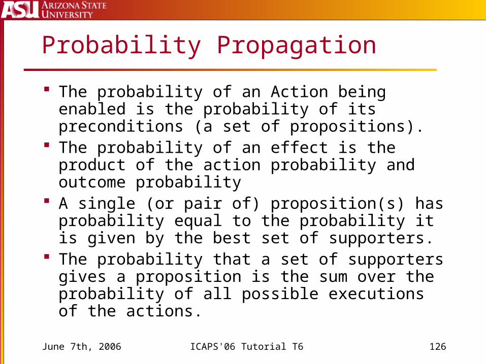
The probability of an Action being enabled is the probability of its preconditions (a set of propositions).
The probability of an effect is the product of the action probability and outcome probability
A single (or pair of) proposition(s) has probability equal to the probability it is given by the best set of supporters.
The probability that a set of supporters gives a proposition is the sum over the probability of all possible executions of the actions.
June 7th, 2006 ICAPS'06 Tutorial T6 127
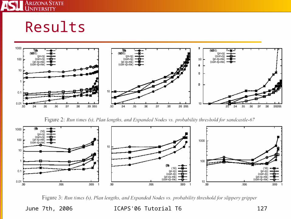
Results
June 7th, 2006 ICAPS'06 Tutorial T6 128
Stochastic Planning Conclusions
Number of joint action outcomes too large Sampling outcomes to represent in labels is
much faster than exact representation SMC gives us a good way to use multiple
planning graph for heuristics, and the McLUG helps keep the representation small
Numeric Propagation of probability can better capture interactions with correlation Can extend to cost and resource propagation
June 7th, 2006 ICAPS'06 Tutorial T6 129
Hybrid Planning Models
June 7th, 2006 ICAPS'06 Tutorial T6 130
Hybrid Models
Metric-Temporal w/ Resources (SAPA) Temporal Planning Graph w/ Uncertainty
(Prottle) PSP w/ Resources (SAPAMPS) Cost-based Conditional Planning (CLUG)
June 7th, 2006 ICAPS'06 Tutorial T6 131
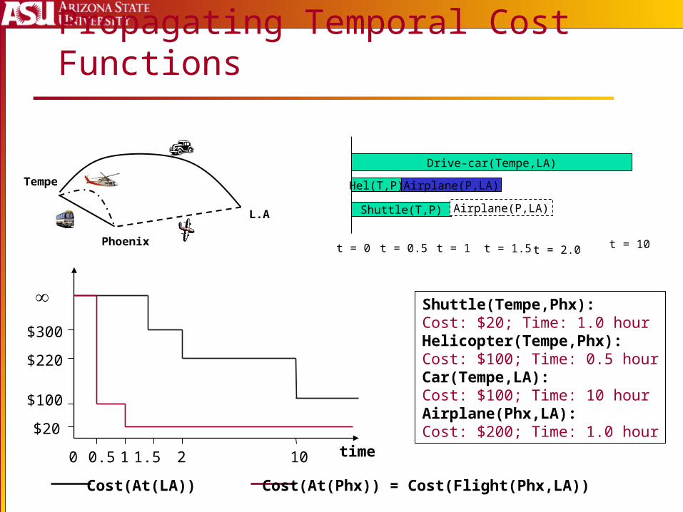
Propagating Temporal Cost Functions
Tempe
Phoenix
L.A
time0 1.5 2 10
$300
$220
$100
t = 1.5 t = 10
Shuttle(Tempe,Phx): Cost: $20; Time: 1.0 hourHelicopter(Tempe,Phx):Cost: $100; Time: 0.5 hourCar(Tempe,LA):Cost: $100; Time: 10 hourAirplane(Phx,LA):Cost: $200; Time: 1.0 hour
1
Drive-car(Tempe,LA)
Hel(T,P)
Shuttle(T,P)
t = 0
Airplane(P,LA)
t = 0.5
0.5
t = 1
Cost(At(LA)) Cost(At(Phx)) = Cost(Flight(Phx,LA))
Airplane(P,LA)
t = 2.0
$20
June 7th, 2006 ICAPS'06 Tutorial T6 132
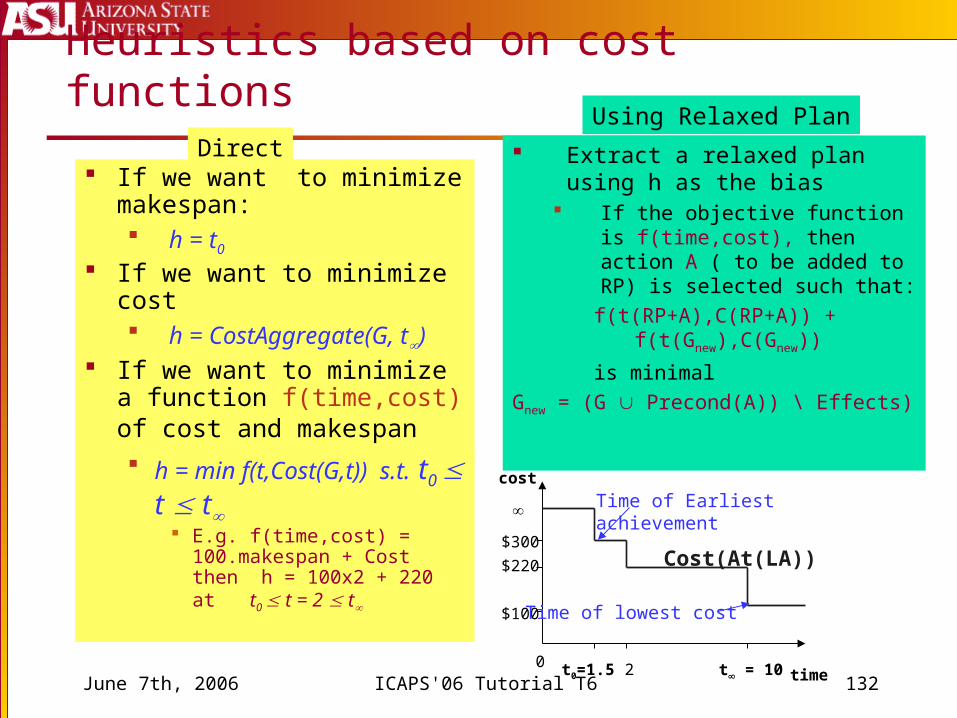
Heuristics based on cost functions
If we want to minimize makespan: h = t0
If we want to minimize cost h = CostAggregate(G, t)
If we want to minimize a function f(time,cost) of cost and makespan h = min f(t,Cost(G,t)) s.t. t0
t t E.g. f(time,cost) =
100.makespan + Cost then h = 100x2 + 220 at t0 t = 2 t
time
cost
0 t0=1.5 2 t = 10
$300
$220
$100
Cost(At(LA))
Time of Earliest achievement
Time of lowest cost
Direct Extract a relaxed plan using h as the bias
If the objective function is f(time,cost), then action A ( to be added to RP) is selected such that:
f(t(RP+A),C(RP+A)) + f(t(Gnew),C(Gnew))
is minimal
Gnew = (G Precond(A)) \ Effects)
Using Relaxed Plan
June 7th, 2006 ICAPS'06 Tutorial T6 133
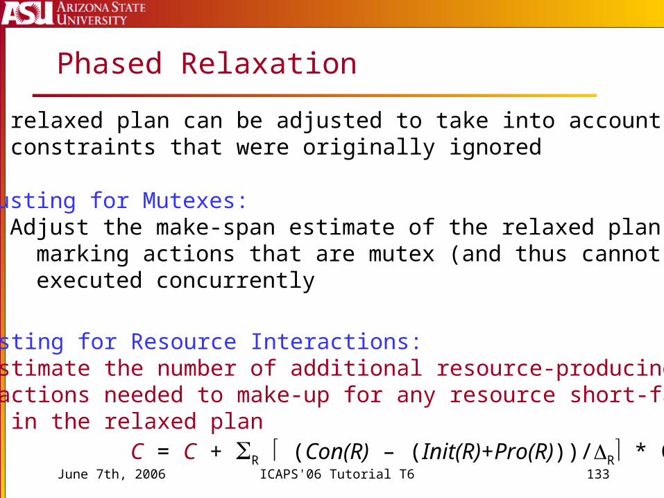
Phased Relaxation
Adjusting for Resource Interactions: Estimate the number of additional resource-producing actions needed to make-up for any resource short-fall in the relaxed plan C = C + R (Con(R) – (Init(R)+Pro(R)))/R * C(AR)
Adjusting for Mutexes: Adjust the make-span estimate of the relaxed plan by marking actions that are mutex (and thus cannot be executed concurrently
The relaxed plan can be adjusted to take into account constraints that were originally ignored
June 7th, 2006 ICAPS'06 Tutorial T6 134
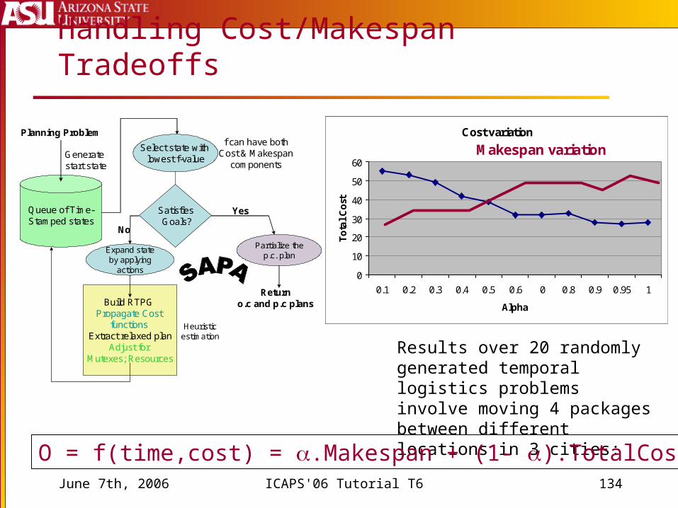
Handling Cost/Makespan Tradeoffs
Results over 20 randomly generated temporal logistics problems involve moving 4 packages between different locations in 3 cities:
O = f(time,cost) = .Makespan + (1- ).TotalCost
Cost variation
0
10
20
30
40
50
60
0.1 0.2 0.3 0.4 0.5 0.6 0 0.8 0.9 0.95 1
Alpha
To
tal
Co
st
Makespan variation
Cost variation
0
10
20
30
40
50
60
0.1 0.2 0.3 0.4 0.5 0.6 0 0.8 0.9 0.95 1
Alpha
To
tal
Co
st
Makespan variation
Build RTPG Propagate Cost
functionsExtract relaxed plan
Adjust for Mutexes; Resources
Planning Problem
Generate start state
No
Partialize thep.c. plan
Returno.c and p.c plans
Expand state by applying
actions
Heuristicestimation
Select state with lowest f-value
SatisfiesGoals?
Queue of Time-Stamped states
Yes
f can have bothCost & Makespan
components
June 7th, 2006 ICAPS'06 Tutorial T6 135
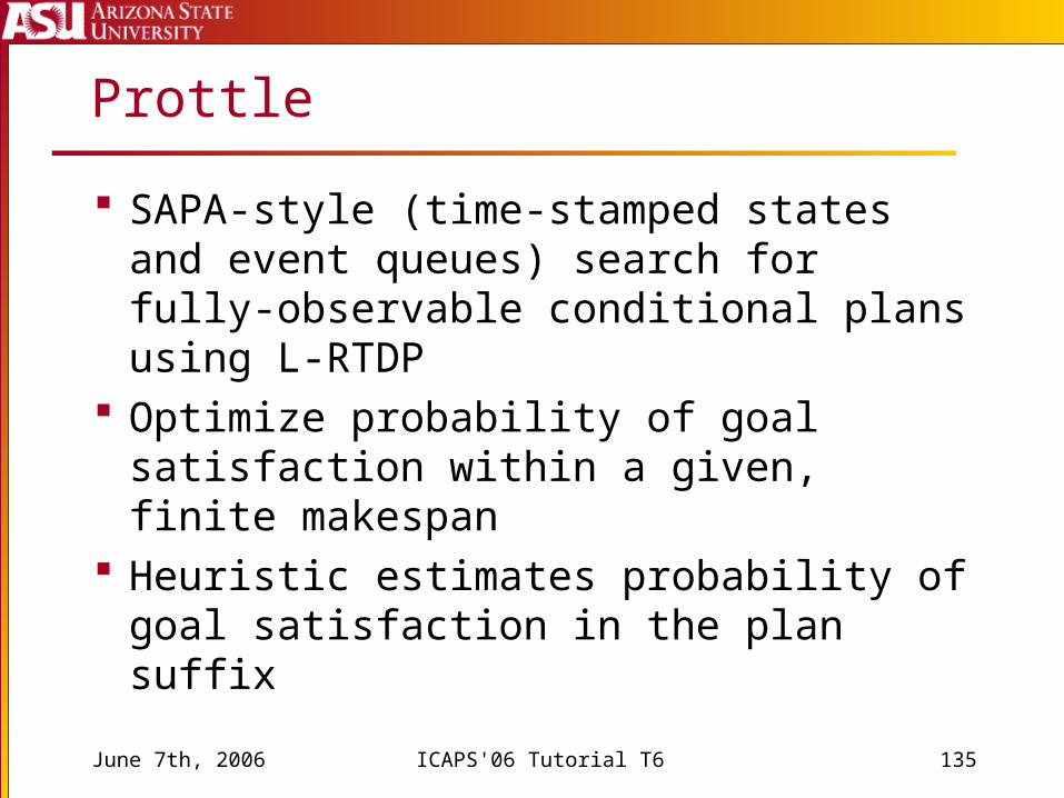
Prottle
SAPA-style (time-stamped states and event queues) search for fully-observable conditional plans using L-RTDP
Optimize probability of goal satisfaction within a given, finite makespan
Heuristic estimates probability of goal satisfaction in the plan suffix
June 7th, 2006 ICAPS'06 Tutorial T6 136
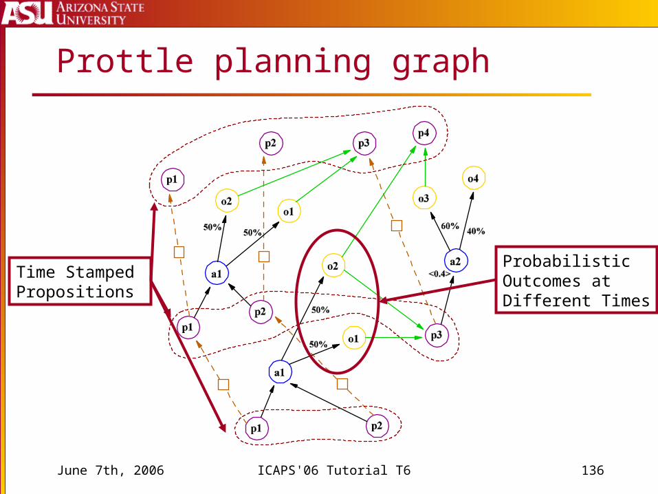
Prottle planning graph
Time Stamped Propositions
ProbabilisticOutcomes atDifferent Times
June 7th, 2006 ICAPS'06 Tutorial T6 137
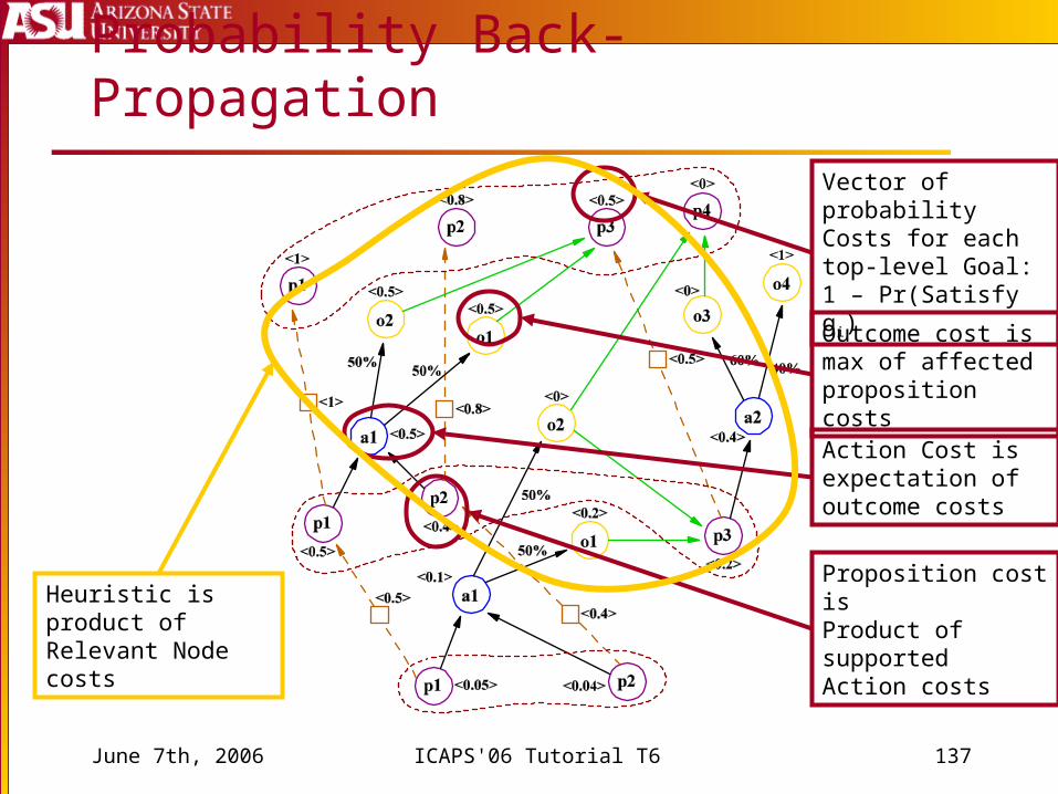
Probability Back-Propagation
Vector of probabilityCosts for each top-level Goal:1 – Pr(Satisfy gi)
Outcome cost is max of affected propositioncosts
Action Cost is expectation of outcome costs
Proposition cost is Product of supported Action costs
Heuristic is product of Relevant Node costs
June 7th, 2006 ICAPS'06 Tutorial T6 138
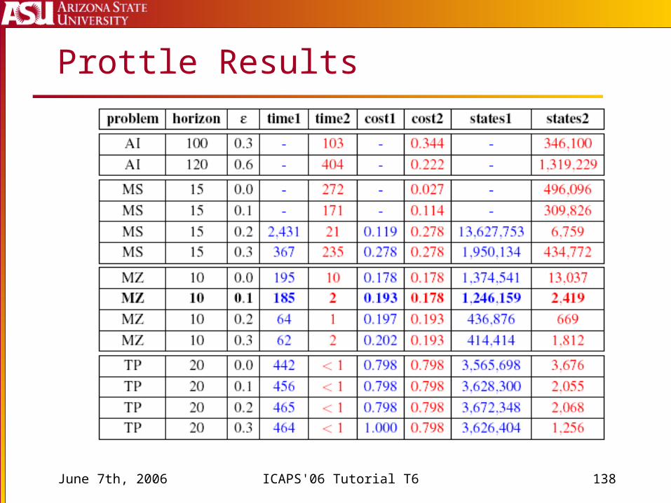
Prottle Results
June 7th, 2006 ICAPS'06 Tutorial T6 139
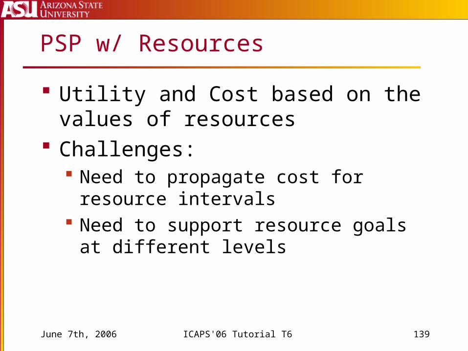
PSP w/ Resources
Utility and Cost based on the values of resources
Challenges: Need to propagate cost for resource intervals Need to support resource goals at different
levels
June 7th, 2006 ICAPS'06 Tutorial T6 140
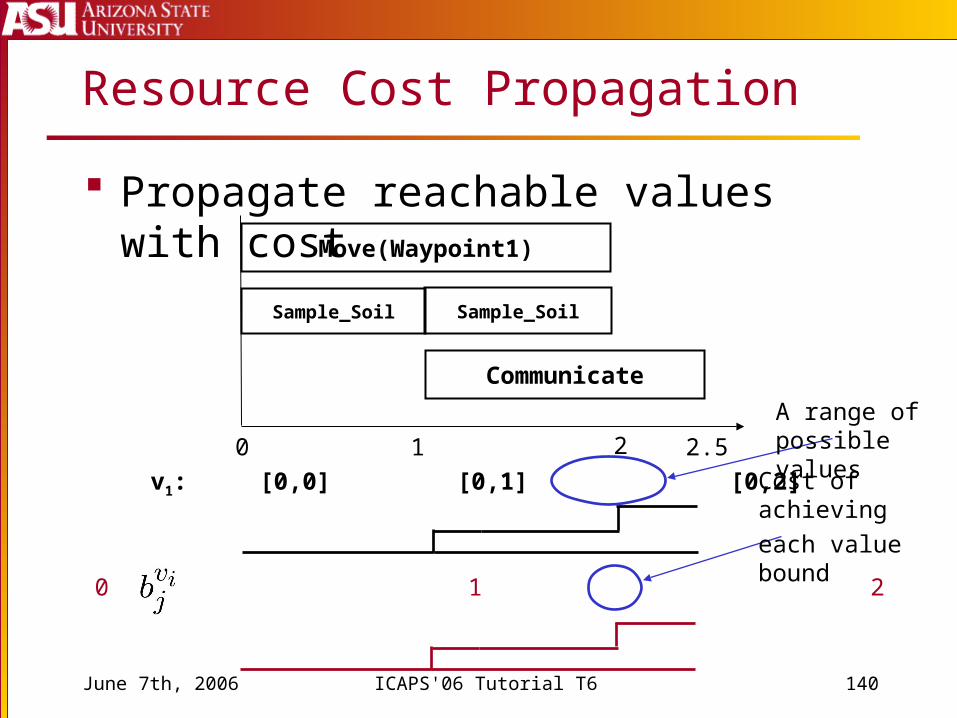
Resource Cost Propagation
Propagate reachable values with cost
Sample_Soil
Communicate
0 1 2 2.5
Move(Waypoint1)
Sample_Soil
cost( ): 0 1 2
Cost of achievingeach value bound
v1: [0,0] [0,1] [0,2]
A range of possible values
June 7th, 2006 ICAPS'06 Tutorial T6 141
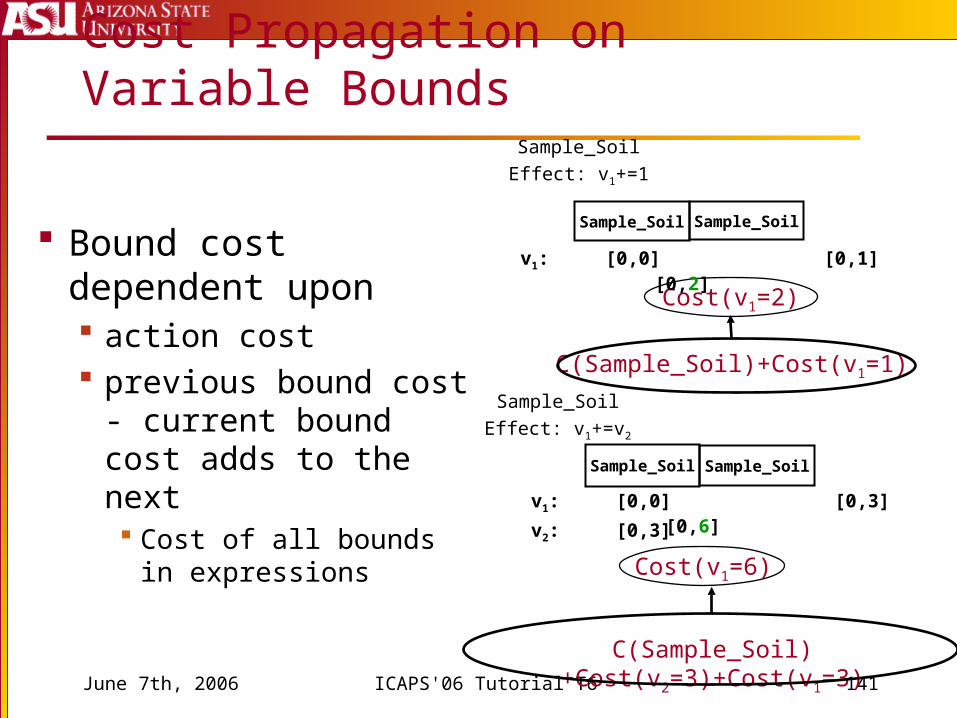
Cost Propagation on Variable Bounds
Bound cost dependent upon action cost previous bound cost
- current bound cost adds to the next Cost of all bounds in
expressions
Sample_Soil
Cost(v1=2)
Sample_Soil
C(Sample_Soil)+Cost(v1=1)
v1: [0,0] [0,1] [0,2]
Sample_Soil
Cost(v1=6)
Sample_Soil
C(Sample_Soil)+Cost(v2=3)+Cost(v1=3)
v1: [0,0] [0,3] [0,6]
v2: [0,3]
Sample_SoilEffect: v1+=1
Sample_SoilEffect: v1+=v2
June 7th, 2006 ICAPS'06 Tutorial T6 142
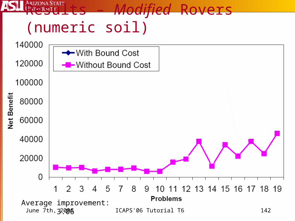
Average improvement: 3.06
Results – Modified Rovers (numeric soil)
June 7th, 2006 ICAPS'06 Tutorial T6 143
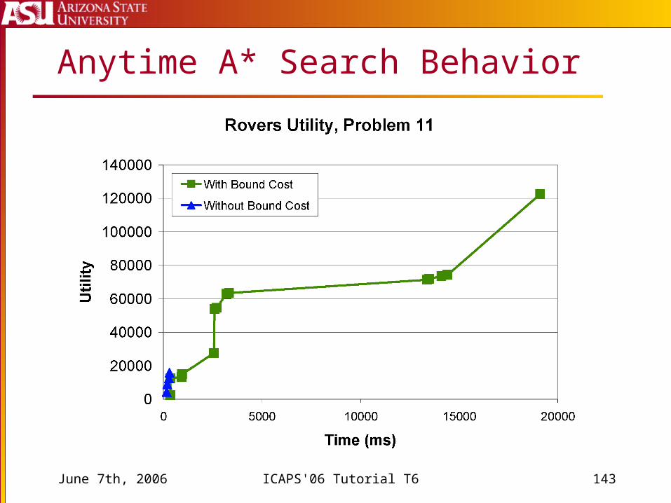
Anytime A* Search Behavior
June 7th, 2006 ICAPS'06 Tutorial T6 144
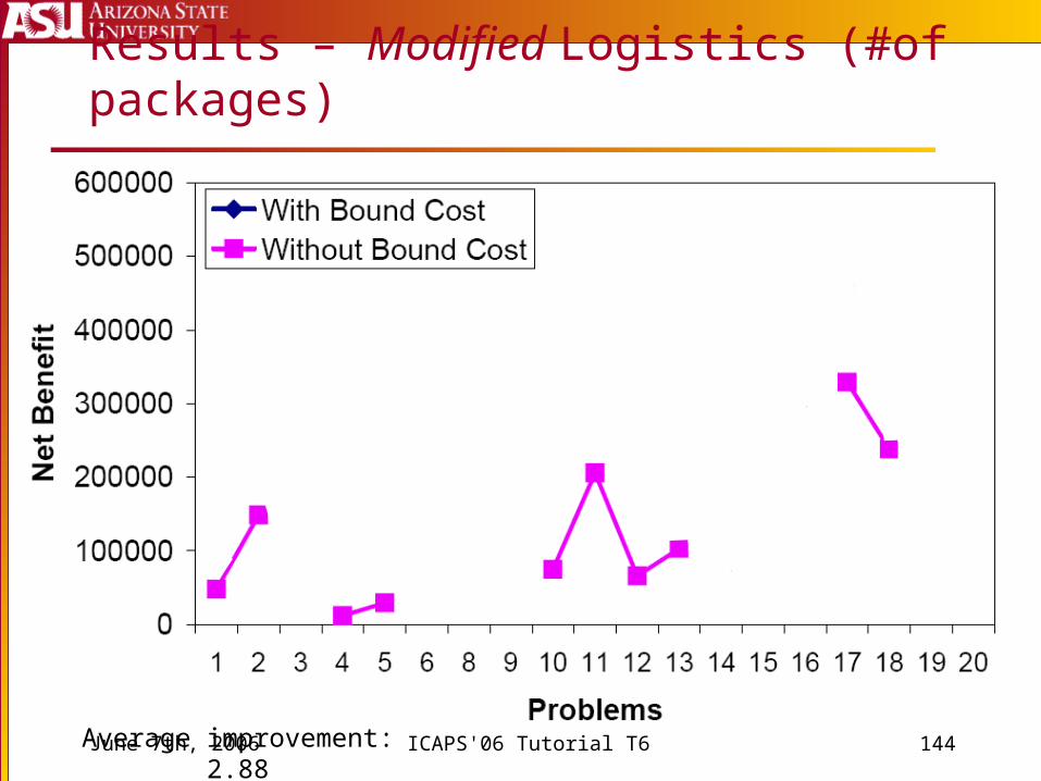
Results – Modified Logistics (#of packages)
Average improvement: 2.88
June 7th, 2006 ICAPS'06 Tutorial T6 145
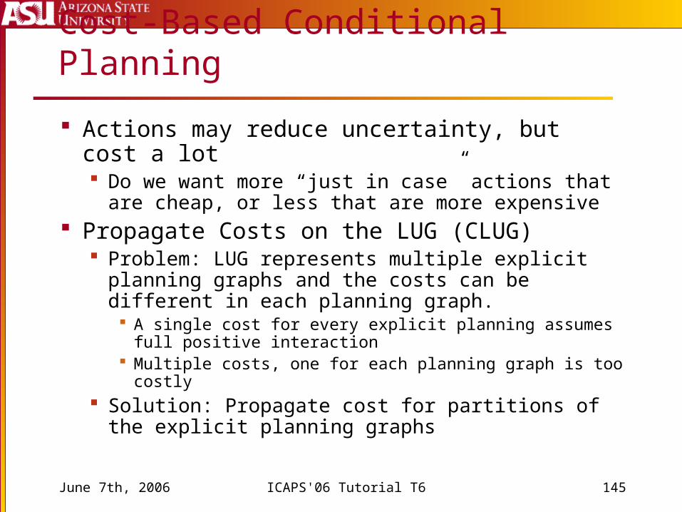
Cost-Based Conditional Planning
Actions may reduce uncertainty, but cost a lot Do we want more “just in case” actions that are cheap,
or less that are more expensive Propagate Costs on the LUG (CLUG)
Problem: LUG represents multiple explicit planning graphs and the costs can be different in each planning graph. A single cost for every explicit planning assumes full positive
interaction Multiple costs, one for each planning graph is too costly
Solution: Propagate cost for partitions of the explicit planning graphs
June 7th, 2006 ICAPS'06 Tutorial T6 146
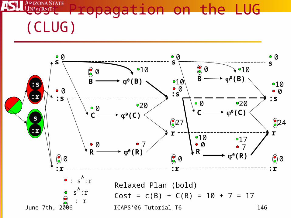
Cost Propagation on the LUG (CLUG)
s
:s
:r
s
:s
r
:r
B
C
R
0(B)
0(C)
0(R)
s
:s
r
:r
B
C
R
0(B)
0(C)
0(R)
: s:rs:r: r
0
0
0
0
0
10
20
0
010
27
0
010
0
0
717
20
10
0
010
0 7
0
24
Relaxed Plan (bold)Cost = c(B) + C(R) = 10 + 7 = 17
:s
:r
s
:r
June 7th, 2006 ICAPS'06 Tutorial T6 147
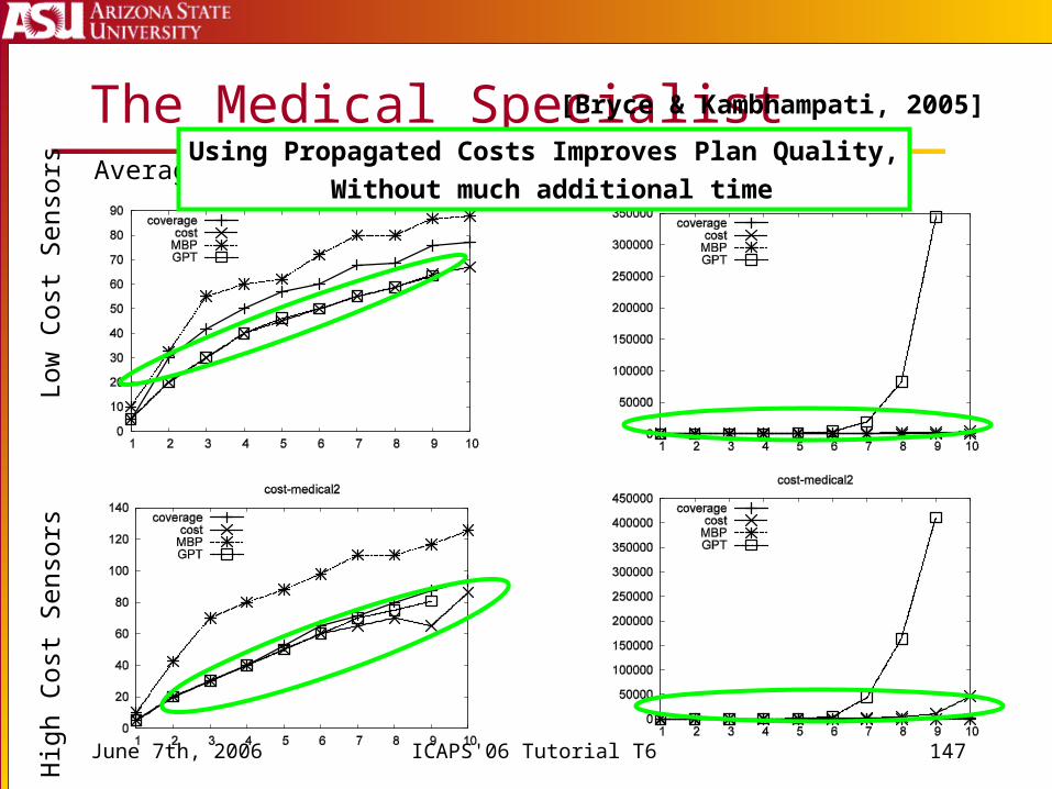
The Medical SpecialistAverage Path Cost Total Time
Hig
h C
ost
Sen
sors
L
ow C
ost
Sen
sors
[Bryce & Kambhampati, 2005]
Using Propagated Costs Improves Plan Quality,
Without much additional time
June 7th, 2006 ICAPS'06 Tutorial T6 148
Overall Conclusions
Relaxed Reachability Analysis Concentrate strongly on positive interactions and
independence by ignoring negative interaction Estimates improve with more negative interactions
Heuristics can estimate and aggregate costs of goals or find relaxed plans
Propagate numeric information to adjust estimates Cost, Resources, Probability, Time
Solving hybrid problems is hard Extra Approximations Phased Relaxation Adjustments/Penalties
June 7th, 2006 ICAPS'06 Tutorial T6 149
Why do we love PG Heuristics?
They work! They are “forgiving”
You don't like doing mutex? okay You don't like growing the graph all the way? okay.
Allow propagation of many types of information Level, subgoal interaction, time, cost, world support, probability
Support phased relaxation E.g. Ignore mutexes and resources and bring them back later…
Graph structure supports other synergistic uses e.g. action selection
Versatility…
June 7th, 2006 ICAPS'06 Tutorial T6 150
PG Variations Serial Parallel Temporal Labelled
Propagation Methods Level Mutex Cost Label
Planning Problems Classical Resource/Temporal Conformant
Planners Regression Progression Partial Order Graphplan-style
Versatility of PG Heuristics