planning and search, model learning, dyna architecture...

Reinforcement Learning

Model-based RL and Integrated Learning-Planning

Planning and Search, Model Learning, Dyna Architecture, Exploration-Exploitation(many slides from lectures of Marc Toussaint & David Silver)

Hung NgoMLR Lab, University of Stuttgart

RL Approaches

Po

lic

y S

ea

rch

Mo

de

l−fr

ee

RL

Mo

de

l−b

as

ed

RL

Inv

ers

e R

L

Imit

ati

on

Le

arn

ing

learn value fct.V (s)

policyπ(s)

optimize policy learn latent costsR(s, a)

dynamic prog.

π(s)policy

learn policyπ(s)

policy

learn model

π(s)

P (s′|s, a)R(s, a)

dynamic prog.V (s) V (s)

π(s)

demonstration dataexperience dataD = {(s, a, r, s′)t}Tt=0 D = {(s0:T , a0:T )d}nd=1

2/53

Outline1. Monte-Carlo planning, MCTS, TD-search2. Model-based RL3. Integrated learning & planning (Dyna)4. Exploration vs. exploitation

– PAC-MDP, artificial curiosity & exploration bonus, Bayesian RL

3/53

1. Monte-Carlo Planning, Tree Search

Online approximate planning for the “now”

4/53

Refresh: Planning with DP Backup

V π(s) = Eπ[rt+1 + γV π(st+1)|st = s

]=∑a π(s, a)

∑s′ P

ass′

[Rass′ + γV π(s′)

]Full-width backup. Iterate for all states

5/53

Heuristic/Forward Search

• Plan for (only) now: use MDP model to look ahead from current state st– Build a search tree with current state st as root node– No need to solve whole MDP; just sub-MDP starting from now

Lecture 8: Integrating Learning and Planning

Simulation-Based Search

Forward Search

Forward search algorithms select the best action by lookahead

They build a search tree with the current state st at the root

Using a model of the MDP to look ahead

T! T! T! T!T!

T! T! T! T! T!

st

T! T!

T! T!

T!T! T!

T! T!T!

No need to solve whole MDP, just sub-MDP starting from now

6/53

Heuristic/Forward Search

• Plan for (only) now: use MDP model to look ahead from current state st– Build a search tree with current state st as root node– No need to solve whole MDP; just sub-MDP starting from now– Backup from leaf nodes; values could be pre-defined.

8.6. HEURISTIC SEARCH 187

by TD-Gammon, but the longer it took to make each move. Backgammon has alarge branching factor, yet moves must be made within a few seconds. It was onlyfeasible to search ahead selectively a few steps, but even so the search resulted insignificantly better action selections.

We should not overlook the most obvious way in which heuristic search focusesbackups: on the current state. Much of the e↵ectiveness of heuristic search is due toits search tree being tightly focused on the states and actions that might immediatelyfollow the current state. You may spend more of your life playing chess than checkers,but when you play checkers, it pays to think about checkers and about your particularcheckers position, your likely next moves, and successor positions. However you selectactions, it is these states and actions that are of highest priority for backups andwhere you most urgently want your approximate value function to be accurate. Notonly should your computation be preferentially devoted to imminent events, butso should your limited memory resources. In chess, for example, there are far toomany possible positions to store distinct value estimates for each of them, but chessprograms based on heuristic search can easily store distinct estimates for the millionsof positions they encounter looking ahead from a single position. This great focusingof memory and computational resources on the current decision is presumably thereason why heuristic search can be so e↵ective.

The distribution of backups can be altered in similar ways to focus on the currentstate and its likely successors. As a limiting case we might use exactly the methods ofheuristic search to construct a search tree, and then perform the individual, one-stepbackups from bottom up, as suggested by Figure 8.12. If the backups are orderedin this way and a table-lookup representation is used, then exactly the same backupwould be achieved as in depth-first heuristic search. Any state-space search can beviewed in this way as the piecing together of a large number of individual one-stepbackups. Thus, the performance improvement observed with deeper searches is not

1 2

3

4 5

6

7

8 9

10

Figure 8.12: The deep backups of heuristic search can be implemented as a sequence ofone-step backups (shown here outlined). The ordering shown is for a selective depth-firstsearch.

• Can we still do fine without having to build an exhaustive search tree?7/53

Refresh: Sample-based Learning

• During learning, the agent samples experience from the real world– real experience: sampled from “true” model, i.e., environment

st+1 ∼ P (s′|st, at); rt+1 ∼ P (r|st, at)

• Then use model-free RL: MC, TD(λ), SARSA, Q-learning, etc.

MC, TD(λ): sample backup.

8/53

Sample-based Planning

• Use the model only to generate samples (as a simulator!)– simulated experience: sampled from the estimated model

st+1 ∼ P̂ (s′|st, at); rt+1 ∼ P̂ (r|st, at)

• Apply model-free RL (MC, TD, Sarsa, Q-learn) to simulated experience

• Sample-based planning methods are often more efficient– Break curse of dimensionality– Computationally efficient, anytime, parallelizable– Works for “black-box” models (only requires samples)

9/53

Simulation-based Search

• Combine forward search + sample-based planning– experience is simulated from now, i.e., from the current real state st

{st, akt , rkt+1, skt+1, . . . , s

kTk}Kk=1 ∼ (M̂, πs)

• Apply model-free RL to simulated episodes: MC search, TD search

10/53

Simple/Flat Monte-Carlo Search

• Given a model M̂ and a (fixed) simulation policy πs (e.g., random)

• For each action a ∈ A: simulate K episodes from current (real) state st

{st, akt , rkt+1, skt+1, . . . , s

kTk}Kk=1 ∼ (M̂, πsim)

• Evaluate actions by average return (Monte-Carlo evaluation)

Q̂(st, a) =1

K

∑k

RktP→ Qπs(st, a) w.r.t. M̂

• Select current (real) action with maximum estimated value

at = arg maxa

Q̂(st, a)

• A “branch” is built but then thrown away.

11/53



MCTS in Go

Monte-Carlo Evaluation in Go

Current position s

Simulation

1 1 0 0 Outcomes

V(s) = 2/4 = 0.5

• Discuss AlphaGo: scale things up!– Value Network pre-trained using expert games– Self-play using MCTS with pre-trained rollout

12/53

Monte-Carlo Tree Search (MCTS)

• Build a search tree during simulated episodes– Caching statistics of rewards and #visits at each (s, a) pair– Used to update a tree policy, e.g., UCT (UCB applied to trees)

πuct(s) = argmaxa

Q̂(s, a) + β

√2 log nsnsa

,∀s ∈ tree

– Outside the current tree: just follow some default rollout policy

• Grow and visit more often the promising & rewarding parts

13/53


• Simulate K episodes following a tree policy and a rollout policy

{st, akt , rkt+1, skt+1, . . . , s

kTk}Kk=1 ∼ (M̂, πktree, π

krollout)

Q̂(s, a) =1

nsa

K∑k=1

Tk∑t′=t

Rkt′(skt′ , a

kt′ |skt′ = s, akt′ = a),∀s ∈ tree

• Greedy tree policy is improved after each simulated episode k– interleaving MC policy-evaluation & policy-improvement in eachsimulated episode– exploit regions of the tree that currently appear better than others– while continuing to explore unknown or less known parts of the tree

• Default/rollout policy: random, pretrained, or learned on realexperience using e.g. model-free off-policy methods

• Converges on the optimal search tree value/policy Q∗(s, a),∀s ∈ tree

14/53




MCTS in Go

Applying Monte-Carlo Tree Search (1)

node(x/y): average return/number of trials

15/53




MCTS in Go


16/53




MCTS in Go


17/53




MCTS in Go


18/53




MCTS in Go


19/53

Monte-Carlo Tree Search (MCTS)8.7. MONTE CARLO TREE SEARCH 189

New node in the tree

Node stored in the tree

State visited but not stored

Terminal outcome

Current simulation

Previous simulation

Figure 3.1: Five simulations of Monte-Carlo tree search.

23

Figure 8.13: Five steps of Monte Carlo Tree Search on a problem with binary returns. Thefirst state added to the tree is the current state St. In this example, the first trajectory endsin a win (a return of 1). In the scond trajectory, the first action is selected the same as before(because it led to a win) and added to the tree. Afterwards the default policy generates therest of the trajectory, which ends in a loss, and the counts in the two nodes within the treeare updated accordingly. The third trajectory then selects a di↵erent first action and endsin a win. The fourth and fifth trajectories repeat this action and end with losses and winsrespectively. Each adds a new node to the tree. Gradually, the tree grows and more actionselections are done (near) greedily within the tree rather than according to the default policy.

20/53

Temporal-Difference Search: Bootstrapping

• MC tree search applies MC control to sub-MDP from now

• TD search applies Sarsa to sub-MDP from now– For each step of simulation, update action-values by Sarsa

∆Q(s, a) = α(r + γQ(s′, a′)−Q(s, a))

• For model-free RL, bootstrapping is helpful– TD learning/search reduces variance but increases bias– TD(λ) learning/search can be much more efficient than MC

21/53

2. Model-based RL

Built once, used forever!

world models outside the context of a decision task [51]. Anumber of cortical areas have also been observed withcorrelates related to model learning [22] and evaluation[34]. Work in learning tasks with task-relevant hiddenstructure may also speak to the construction of worldmodels [52]. These studies have implicated the lateralPFC, an area often associated with working memoryfunction, in discovery of this structure.

The way forwardWhy the ubiquity of evidence for model-based RL?Several factors probably contribute, all of which pointto important opportunities for progress.

First, the resolution and other limitations of the BOLDsignal may conceal distinctions that would be visibleusing more invasive techniques. The explosion of humanstudies explicitly examining model-based RL is recentenough that analogous animal electrophysiological stu-dies are largely not yet available. A strength of fMRI is todevelop tasks and analyses, and to locate areas for furtherstudy; the time is now ripe to test similar tasks in animals.For instance, further dissociations might be found in thesignaling properties of different DA cell groups andprojections [23], potentially elucidating the potentialco-expression of model-based and model-free signalsby DA cells.

Second, the brain’s RPE systems may be smarter thanthey have been made out to be, yet still essentially model-free. Of the different characteristics that have been takenas hallmarks of model-based RL, some are easier thanothers to accommodate in a lightly modified model-free

system. In particular, a model-free learner can generalizelearning from one state to another, without additionalexperience, if its inputs corresponding to those statesoverlap (Figure 2). This is a particularly plausible expla-nation for seemingly model-based inference in serialreversal and similar tasks [40,41,44], as indeed the authorsof some of these studies have pointed out. If counter-factual updating in these tasks occurs implicitly, due togeneralization, then it would not involve forward model-ing of future states. In this respect, tasks involvingsequential contingencies are stronger and more canonicaltests of model-based RL, but variants of the same repres-entational trick can in principle apply even there [53]. Forinstance, if actions are represented in terms of theirassociated outcomes — for instance, if the representationfor a lever that produces food overlaps with that for thefood itself — and if these inputs (themselves now, ineffect, a sort of world model) are mapped to values usingeven model-free RL, then the learned value will besubstantially shared between the lever and the food. Inthis case, if the food is devalued, the lever-press value willalso decline immediately, and the resulting behavior willappear goal-directed. This approach might help toexplain the involvement of similar striatal circuits in bothgoal-directed and habitual behavior. More elaborate ver-sions of this scheme can apply to arbitrary sequentialtasks, but such a strategy is easier to spot, and potentiallyto rule out, in tasks with deeper sequential structure andchanging transition contingencies [34].

Third, there may be hitherto unanticipated crosstalk orintegration between model-based and model-free sys-tems. It is reasonable to imagine that model-based

4 Decision making

CONEUR-1112; NO. OF PAGES 7

Please cite this article in press as: Doll BB, et al.: The ubiquity of model-based reinforcement learning, Curr Opin Neurobiol (2012), http://dx.doi.org/10.1016/j.conb.2012.08.003

Figure 2

+

δ

--+

Current Opinion in Neurobiology

Learning through value generalization (left) and model-based forward planning (right). In a reversal learning task (left), the rat has just taken an action(lever-press) and received no reward, and so updates its internal choice value representation to decrement the chosen value’s option. Because theunchosen value’s option is represented on the same scale, inverted, it is implicitly incremented as well. Implemented this way, learning relies onmodel-free updating over a modified input, and does not involve explicitly constructing or evaluating a forward model of action consequences. In amodel-based RL approach to a maze task (right), the rat has an internal representation of the sequential structure of the maze, and uses it to evaluate acandidate route to the reward.

Current Opinion in Neurobiology 2012, 22:1–7 www.sciencedirect.com

22/53

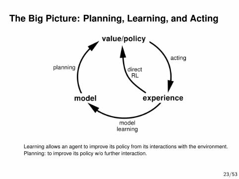
The Big Picture: Planning, Learning, and Acting

Learning allows an agent to improve its policy from its interactions with the environment.Planning: to improve its policy w/o further interaction.

23/53

Model-based RL

• Model learning: given experience D = {(st, at, rt+1, st+1)}Ht=1

– learning P (s′, r|s, a): regression/density estimation problems

– discrete state-action space: counting, P̂ (s′|s, a) =ns′sa

nsa

– continuous state-action space: P̂ (s′|s, a) = N (s′ |φ(s, a)>β,Σ)

estimate parameters β (and perhaps Σ) as for regression

– D as a model: experience replay!

• Example: linear forward model, φ(s′) = Faφ(s); r = b>a φ(s)

– Least mean squares (LMS) SGD update rule:

F ← F + α(φ(s′)− Fφ(s))φ(s)>; b← b+ α(r − b>φ(s))φ(s)

• To construct V ∗/π∗ from learned model: use planning– discrete case: DP on the estimated model (VI, PI, etc.)– sample-based planning (MCTS, TD-search): simple but powerful– continuous case: differential DP; planning-by-inference, etc.

24/53

Model-based RL

• Model learning: given experience D = {(st, at, rt+1, st+1)}Ht=1

– learning P (s′, r|s, a): regression/density estimation problems

– discrete state-action space: counting, P̂ (s′|s, a) =ns′sa

nsa

– continuous state-action space: P̂ (s′|s, a) = N (s′ |φ(s, a)>β,Σ)

estimate parameters β (and perhaps Σ) as for regression– D as a model: experience replay!

• Example: linear forward model, φ(s′) = Faφ(s); r = b>a φ(s)

– Least mean squares (LMS) SGD update rule:

F ← F + α(φ(s′)− Fφ(s))φ(s)>; b← b+ α(r − b>φ(s))φ(s)

• To construct V ∗/π∗ from learned model: use planning– discrete case: DP on the estimated model (VI, PI, etc.)– sample-based planning (MCTS, TD-search): simple but powerful– continuous case: differential DP; planning-by-inference, etc.

24/53

Model-based RL: Pros and Cons

• Advantages:– Can efficiently learn model by supervised learning methods– Rapid adaptation to new problems and situations (via planning)– Can reason about model uncertainty

• Disadvantages: two sources of approximation error!– In estimating model and value function– If model is inaccurate⇒ planning will compute a suboptimal policy– Hence, asymptotically model-free methods are often better– Solution 1: reason explicitly about model uncertainty (BRL)– Solution 2: use model-free RL when model is wrong– Solution 3: integrated model-based and model-free

25/53



• Disadvantages: two sources of approximation error!– In estimating model and value function– If model is inaccurate⇒ planning will compute a suboptimal policy– Hence, asymptotically model-free methods are often better

– Solution 1: reason explicitly about model uncertainty (BRL)– Solution 2: use model-free RL when model is wrong– Solution 3: integrated model-based and model-free

25/53



• Disadvantages: two sources of approximation error!– In estimating model and value function– If model is inaccurate⇒ planning will compute a suboptimal policy– Hence, asymptotically model-free methods are often better– Solution 1: reason explicitly about model uncertainty (BRL)– Solution 2: use model-free RL when model is wrong– Solution 3: integrated model-based and model-free

25/53

3. Integrated Learning & Planning: Dyna

Combining the best of both worlds!

Reinforcement learning: The Good, The Bad and The Ugly Dayan and Niv 187

Box 1 Model-based and model-free reinforcement learning

Reinforcement learning methods can broadly be divided into two classes, model-based and model-free. Consider the problem illustrated in thefigure, of deciding which route to take on the way home from work on Friday evening. We can abstract this task as having states (in this case,locations, notably of junctions), actions (e.g. going straight on or turning left or right at every intersection), probabilities of transitioning from onestate to another when a certain action is taken (these transitions are not necessarily deterministic, e.g. due to road works and bypasses), andpositive or negative outcomes (i.e. rewards or costs) at each transition from scenery, traffic jams, fuel consumed, etc. (which are againprobabilistic).

Model-based computation, illustrated in the left ‘thought bubble’, is akin to searching a mental map (a forward model of the task) that has beenlearned based on previous experience. This forward model comprises knowledge of the characteristics of the task, notably, the probabilities ofdifferent transitions and different immediate outcomes. Model-based action selection proceeds by searching the mental map to work out the long-run value of each action at the current state in terms of the expected reward of the whole route home, and chooses the action that has the highestvalue.

Model-free action selection, by contrast, is based on learning these long-run values of actions (or a preference order between actions) withouteither building or searching through a model. RL provides a number of methods for doing this, in which learning is based on momentaryinconsistencies between successive estimates of these values along sample trajectories. These values, sometimes called cached values becauseof the way they store experience, encompass all future probabilistic transitions and rewards in a single scalar number that denotes the overall futureworth of an action (or its attractiveness compared with other actions). For instance, as illustrated in the right ‘thought bubble’, experience may havetaught the commuter that on Friday evenings the best action at this intersection is to continue straight and avoid the freeway.

Model-free methods are clearly easier to use in terms of online decision-making; however, much trial-and-error experience is required to make thevalues be good estimates of future consequences. Moreover, the cached values are inherently inflexible: although hearing about an unexpectedtraffic jam on the radio can immediately affect action selection that is based on a forward model, the effect of the traffic jam on a cached propensitysuch as ‘avoid the freeway on Friday evening’ cannot be calculated without further trial-and-error learning on days in which this traffic jam occurs.Changes in the goal of behavior, as when moving to a new house, also expose the differences between the methods: whereas model-baseddecision making can be immediately sensitive to such a goal-shift, cached values are again slow to change appropriately. Indeed, many of us haveexperienced this directly in daily life after moving house. We clearly know the location of our new home, and can make our way to it byconcentrating on the new route; but we can occasionally take an habitual wrong turn toward the old address if our minds wander. Suchintrospection, and a wealth of rigorous behavioral studies (see [15], for a review) suggests that the brain employs both model-free and model-baseddecision-making strategies in parallel, with each dominating in different circumstances [14]. Indeed, somewhat different neural substrates underlieeach one [17].

www.sciencedirect.com Current Opinion in Neurobiology 2008, 18:185–196

26/53

Dyna: Integrating Learning and Planning

• Model-free RL– No model– Learn value function (and/or policy) from real experience

• Model-based RL (using sample-based planning)– Learn a model from real experience– Plan value function/policy from simulated experience

• Dyna– Learn a model from real experience– Learn & plan value function/policy from real & simulated experience

27/53

The Dyna Architecture

• Two distributions of states and actions (experience)– Learning distribution (real experience)– Search distribution (simulated experience)

• Integrated approaches differ in generating search distributions– simulated transitions: Dyna-Q, Dyna+Priority Sweeping– simulated trajectories from TD-search: Dyna-2

28/53

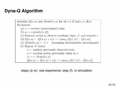
Dyna-Q Algorithm

steps (a–e): real experience; step (f): in simulation

29/53

Dyna-Q Algorithm: Example on Simple Maze

Introduction to RL, Sutton & Barto, 1998

30/53

Dyna-Q Algorithm: 1st and 2nd Episode

Introduction to RL, Sutton & Barto, 1998

31/53

When the Model Is Wrong: Changed Environment

The changed environment is harder

32/53

When the Model Is Wrong: Short-cut Maze

The changed environment is easier

33/53

Dyna-Q+

• This agent keeps track for each state-action pair of how many timesteps tsa have elapsed since the pair was last tried in a real interaction.

• If the transition has not been tried in tsa time steps: assigned a“phantom” reward (exploration bonus) r + κ

√tsa, for small κ

– on simulated experiences involving these actions– To encourage behavior that tests long-untried actions

• A form of artificial/computational “curiosity”, “intrinsic” rewards– the agent motivates itself to visit long unvisited states

34/53

4. Exploration vs. Exploitation

(Too much) curiosity kills the cat!

35/53

https://vimeo.com/49152310

Exploration vs. Exploitation Dilemma

• RL agents start to act without a model of the environment: have tolearn from its experience what to do in order to fulfill tasks andachieve high average return.

• Online decision-making involves a fundamental choice:– Exploitation: Make the best decision given current information– Exploration: Gather more information

• The best long-term strategy may involve short-term sacrifices

• Gather enough information to make the best overall decisions⇒ exploration as fundamental intelligent behavior

36/53

Exploration: Motivating Example

37/53

Exploration Strategies/Principles

• Naive Exploration– Add noise to greedy policy (e.g. ε-greedy)

• Optimistic Initialization– Assume the best until proven otherwise

• Optimism in the Face of Uncertainty– Prefer actions with uncertain values (e.g., UCB: µ̂sa + β

√2 logns

nsa)

• Probability Matching– Select actions according to probability they are best

• Information State Search– Lookahead search incorporating value of information (e.g., BRL)

• Other heuristics– Recency-based exploration bonus for non-stationary environment

• Need a notion of optimality: sample complexity

38/53

Sample Complexity

• Let M be an MDP with N states, K actions, discount factor γ ∈ [0, 1)

and a maximal reward Rmax > 0.

• Let A be an algorithm (that is, a reinforcement learning agent) that actsin the environment, resulting in ht = (s0, a0, r1, s1, a1, r2, . . . , rt, st).

• Let V At,M = E[∑∞

i=0 γirt+i |ht

]; V ∗ is the optimal value function.

• Define an accuracy threshold ε: ‖V̂ − V ∗‖ ≤ ε

39/53

Sample Complexity and Efficient Exploration

• Definition (Kakade, 2003):Let ε > 0 be a prescribed accuracy and δ > 0 be an allowed probabilityof failure. The expression η(ε, δ,N,K, γ,Rmax) is a sample complexitybound for algorithm A if independently of the choice of s0, withprobability at least 1− δ, the number of timesteps such thatV At,M < V ∗(st)− ε is at most η(ε, δ,N,K, γ,Rmax).

• An algorithm with sample complexity that is polynomial in 1/ε, log(1/δ),N , K, 1/(1− γ), Rmax is called PAC-MDP (probably approximatelycorrect in MDPs).

40/53

Sample Complexity of Exploration Strategies

• Assume we have estimates Q̂(s, a)

• ε-greedy: π(s) =

argmaxa Q̂(s, a) with probability 1− εrandom action with probability ε

– Most popular method– Converges to the optimal value function with probability 1 (all pathswill be visited sooner or later), if the exploration rate diminishesaccording to an appropriate schedule.– Problem: sample complexity exponential in the number of states

• Boltzmann: choose action a with softmax probabilities exp(Q̂(s,a)/T )∑a exp(Q̂(s,a)/T )

– Temperature T controls amount of exploration– Problem again: sample complexity exponential in #states

41/53

Sample Complexity of Exploration Strategies

• Other heuristics for exploration:– minimize variance of action value estimates– optimistic initial values (“optimism in the face of uncertainty”)– state bonuses: frequency, recency, error etc.⇒ Again: sample complexity exponential in #states

• Bayesian RL: optimal exploration strategy– maintain a probability distribution over MDP models (i.e., parameters)– posterior distribution updated after each new observation (interaction)– exploration strategy minimizes uncertainty of parameters– Bayes-optimal solution to the exploration-exploitation tradeoff (i.e., noother policy is better in expectation w.r.t. prior distribution over MDPs)– only tractable for very simple problems

42/53

PAC-MDP Algorithms

• Explicit-Exploit-or-Explore (E3) & RMAX– principled approach to the exploration-exploitation tradeoff withpolynomial sample complexity

• Common intuition: again, optimism in the face of uncertainty– If faced the option of certain and uncertain reward regions, try theuncertain reward region!

43/53

Explicit-Exploit-or-Explore (E3)

• Model-based PAC-MDP (Kearns & Singh ’02)– Assuming maximum reward Rmax is known

• Quantify confidence in model estimates– Maintaining counts for executed state-action pairs– A state s is known if ∀a ∈ A(s) have been executed sufficiently often.

• From observed data, E3 constructs two MDPs:

– MDPknown: includes known states with (approximately exact)estimates of P (st+1 | at, st) and P (rt+1 | at, st)→ for exploiting!

– MDPunknown: MDPknown + special state s? with “self-loop” where theagent receives maximum reward→ for exploring!

44/53

E3 Sketch

Input: State sOutput: Action a

if s is known thenPlan in MDPknown B Sufficiently accurate model estimatesif resulting plan has value above some threshold then

return first action of plan B Exploitationelse

Plan in MDPunknown

return first action of plan B Planned explorationelse

return action with the least observations in s B Direct exploration

45/53

E3 Example

S. Singh (Tutorial 2005)

46/53

E3 Example

47/53

E3 Example

M : true known state MDP M̂: estimated known state MDP

48/53

E3 Implementation Setting

• T is the time horizon

• GTmax is the maximum T-step return. (discounted case GTmax ≤ TRmax)

• A state is known if it was visited O(

(NTGTmax/ε)4νmax log(1/δ)

)times.

(νmax is the maximum variance of the random payoffs over all states)

• For the exploration/exploitation choice at known states: It’s assumed tobe given the optimal value function V ∗. If V̂ obtained from theMDPknown > (V ∗ − ε) then do exploitation.

49/53

RMAX Algorithm

• R-MAX solves only one unique model (no separate MDPknown andMDPunknown) and therefore implicitly explores or exploits.

• R-MAX and E3 algorithms achieve roughly the same level ofperformance (Strehl’s thesis).

• RMAX builds an approximate MDP based on reward function

R(s, a) =

R̂(s, a) if (s,a) known depending on some parameter m

Rmax otherwise

50/53

RMAX’s Pseudocode

Inputs: S,A, Rmax,m.

// Initialization: all transitions are to “heaven” and maximally rewarding!

Add “heaven state” s∗ to the state space: S ′ = S ∪ {s∗}.Initialize R̂(s, a) = Rmax, T̂ (s

′|s, a) = δs′(s∗) for all s, s′ ∈ S ′.

// Kronecker function δs′(s∗) = 1 if s′ = s∗, and 0 otherwise.

Initialize a uniform random policy π.Initialize all couters n(s, a) = 0;n(s, a, s′) = 0; r(s, a) = 0, ∀s ∈ S, s′ ∈ S ′, a ∈ A.

while not converged do// Select action randomly until first time model update.Execute a = π(s), observe s′, r.Update n(s, a)← n(s, a) + 1;n(s, a, s′)← n(s, a, s′) + 1; r(s, a)← r(s, a) + r.if n(s, a) = m then

// For small domains we can use n(s, a) ≥ mUpdate T̂ (·|s, a) = n(s, a, ·)/n(s, a), and R̂(s, a) = r(s, a)/n(s, a).Update policy π using MDP model (T̂ , R̂) // e.g., Q-Iteration.

51/53

RMAX Analysis

• (Upper bound) There exists m = O(NT 2

ε2 ln2 NKδ

), then with probability

of at least 1− δ, V (st) ≥ V ∗(st)− ε is true for all but

O

(N2KT 3

ε3ln2 NK

δ

)

steps, where N is the number of states.

• For discounted case: T = − log ε1−γ

• The general PAC-MDP theorem is not easily adapted to the analysis ofE3 because of its use of two internal models– Original analysis depends on horizon and mixing time

52/53

Limitations of E3 and RMAX• E3 and RMAX are called “efficient” because their sample complexity is

only polynomial in the number of states.• This is usually too slow for practical algorithms but is probably the best

that can be done in the worst case.• In natural environments the number of states is enormous:

exponential in the number of objects in the environment.• Hence E3/RMAX sample complexity scales exponentially in the

number of objects.

• Generalization over states and actions is crucial for exploration– Exploration in relational RL (Lang & Toussaint ’12) 53/53

planning and search, model learning, dyna architecture...

Documents