planning and execution of straight line manipulator ...rht/rht papers/1979/straight line...

Russell H. Taylor

Planning and Execution of Straight Line Manipulator Trajectories

Recently developed manipulator control languages typically specify motions as sequences ofpoints through which a tool afixed to the end of the manipulator is to pass. The effectiveness of such motion specijication formalisms is greatly increased if the tool moves in a straight line between the user-specijied points. This paper describes two methods for achieving such straight line motions. The first method is a refinement of one developed in 1974 by R . Paul. Intermediate points are interpolated along the Cartesian straight line path at regular intervals during the motion, and the manipulator’s kinematic equations are solved to produce the corresponding intermediate joint parameter values. The path interpolation functions developed here offer several advantages, including less computational cost and improved motion characteristics. The second method uses a motion planning phase to precompute enough intermediate points so that the manipulator may be driven by interpolation of joint parameter values while keeping the tool on an approximately straight line path. This technique allows a substantial reduction in real time computation and permits problems arising from degenerate joint alignments to be handled more easily. The planning is done by an eficient recursive algorithm which generates only enough intermediate points to guarantee that the tool’s deviation from a straight line path stays within prespecijied error bounds.

Introduction Over the past ten years, general purpose automation machines consisting of a sequence of motor driven links, or “joints,” operating under control of a computer have be- gun to appear in industry. These “manipulators” generally terminate in a gripper-like hand or other tool and can be used for assembly, parts handling, welding, and many other applications.

The development of these devices requires both provi- sion of suitable formalisms for describing the motions to be made and implementation of suitable control strategies for carrying them out. The simplest approach is to record the values of the joint parameters which place the hand at particular desired points and then to move the joints inde- pendently from one set of parameters to the next. More sophisticated motion execution schemes (e.g . , [ 1-31) frequently include an open loop trajectory component that generates intermediate target values for the joints. These

schemes are often accompanied by more sophisticated means of describing the desired motion to be made.

Of particular interest has been the development of programming languages [4-71 in which manipulator target points are described by transformations relating the coordinate system of the hand or tool to the coordinate system of the work station. Motions in these languages are specified as sequences of “knot” points through which the controlled frame is to pass. The joint vectors corresponding to each Cartesian knot point are computed by solving the link equations for the manipulator, which are then used by the motion execution programs. One drawback to this scheme is that it leaves undefined the precise path taken by the manipulator between knot points. This makes programming more difficult, since it is hard to predict just how many intermediate points should be added to a motion statement and complicates the de-

Copyright 1979 by International Business Machines Corporation. Copying is permitted without payment of royalty provided that ( 1 ) each reproduction is done without alteration and (2) the Journal reference and IBM copyright notice are included on the first page.

424 The title and abstract may be used without further permission in computer-based and other information-service systems. Permission to republish other excerpts should be obtained from the Editor.

RUSSELL n. TAYLOR IBM J . RES. DEVELOP. VOL. 23 NO. 4 JULY 1919

velopment of model-based program automation tools [ 5 , 71.

One obvious motion strategy is to cause the hand or tool to move along a straight line path between knot points. Whitney [8] achieved differential straight line motions in 1968 by multiplying the inverse Jacobean of the manipulator’s joint to Cartesian space transformation by a desired motion increment vector. By repeated evalua- tion of the inverse Jacobean, this technique can be used to produce long straight line motions. In 1974, Paul [9] implemented a rather more straightforward technique, in which intermediate Cartesian space goals are evaluated every 100 ms during motion execution. The manipulator link equations are then solved to produce intermediate joint goals.

This paper discusses two approaches to the problem of straight line motion between knot points. The first approach is similar to Paul’s. However, a number of refine- ments are presented which permit the path functions to be evaluated somewhat more efficiently, provide more uniform rotational motions, and allow “tracking” of real time changes in the knot points. Although the method is flexible and conceptually straightforward, it requires con- siderable real time computation and is vulnerable to degenerate configurations of the manipulator’s joints. In the second approach, a motion planning phase adds enough intermediate points so that the manipulator may be controlled by linear interpolation of joint values without allowing the hand to deviate more than a prespecified amount from a straight line Cartesian path. This substantially reduces the amount of real time computation required to drive the machine and permits problems arising from degenerate joint alignments to be handled more easily.

Notational conventions We assume that the manipulator’s motion is specified by a sequence of “frame” transformations giving the location and orientation of the hand with respect to the coordinate system of the work station. Each such frame Fi consists of a rotation Ri followed by translation by a displacement vector p i . Frames may be composed by “multiplication” on the left, where

rotation part ( F , o F,) = R1o R,,

translation part (F1 0 F,) = R , 0 p , + p ,

For instance, if FA gives the location and orientation of an object A with respect to the work station and p , is the location of a point with respect to the origin of A, then the location of the point with respect to the work station is

given by

P , = R,OP, + P A .

Similarly, if R, gives the orientation of a feature with respect to A, then its orientation with respect to the work station is

R , = R,o R, .

We frequently express a rotation R as a “right-handed” twist by an angle 0 about an axis n:

R = Rot(n, 0).

From this definition, it follows that

R” = Rot(n, -0) = Rot( -n , 0).

Frame transformations are commonly represented as 4 X

4 matrices:

Rl, R, , R, , P I

R,,

This representation is easy to understand and use, since frames may be composed using the ordinary rules for matrix multiplication. Also, since rotation matrices have the property that their inverse is the same as their transpose,

the inverse transformation for a frame is easily computed.

On the other hand, there are several disadvantages to the use of matrix representations. The matrices are mod- erately expensive to store, and computations on them require more operations than for some other representations. Also, since the representation of rotations is highly redundant, numerical inconsistencies can be a problem, so that occasional renormalization may be necessary.

Quaternions [ lo , 1 1 1 offer another convenient representation for rotations and have been applied extensively to the analysis of kinematic linkages [12]. The quaternion corresponding to a rotation by angle 0 about axis n is

Rot(n, 0) = [cos (3 + sin (3 . n ] .

For our purposes, this representation is rather more ef- ficient than the matrix representation. Storage requirements are reduced, and calculations involving rotations can be done with fewer primitive operations (adds and multiplies) than are required if matrices are used. Appen- dix A provides a brief review of quaternions and includes a table comparing the computational requirements of quaternion and matrix representations for rotations. 425

RUSSELL n. TAYLOR IBM J. RES. DEVELOP, VOL. 23 NO. 4 JULY 1979

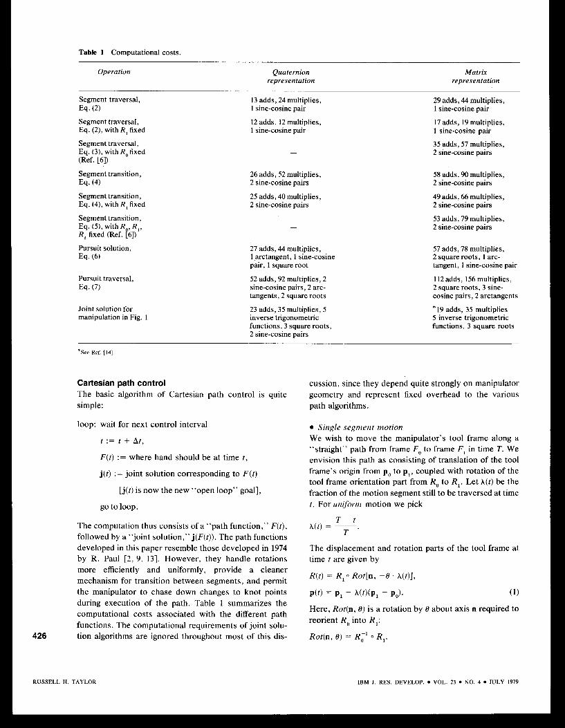
Table 1 Computational costs.

Operation Quaternion representation

Matrix representation

Segment traversal, Eq. (2)

Segment traversal, Eq. (2), with R, fixed

Segment traversal, Eq. (3), with R,fixed (Ref. [61)

Eq. (4) Segment transition,

Segment transition, Eq. (4), with R, fixed

Segment transition, Eq. ( 3 , with R , R , , R, fixed (Ref. f6])

Pursuit solution, Eq. (6)

Pursuit traversal, Eq. (7)

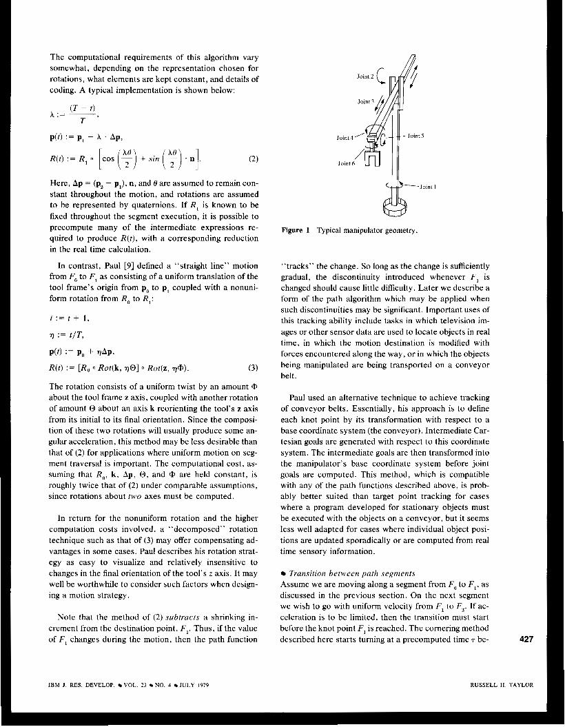
Joint solution for manipulation in Fig. 1

13 adds, 24 multiplies, 1 sine-cosine pair


26 adds, 52 multiplies, 2 sine-cosine pairs


27 adds, 44 multiplies, 1 arctangent, 1 sine-cosine pair, 1 square root

52 adds, 92 multiplies, 2 sine-cosine pairs, 2 arctangents, 2 square roots

23 adds, 35 multiplies, 5 inverse trigonometric functions, 3 square roots, 2 sine-cosine pairs







57 adds, 78 multiplies, 2 square roots, 1 arctangent, 1 sine-cosine pair

112 adds, 156 multiplies, 2 square roots, 3 sine- cosine pairs, 2 arctangents

*19 adds, 35 multiplies 5 inverse trigonometric functions, 3 square roots

*See Ref. [I41

Cartesian path control cussion, since they depend quite strongly on manipulator The basic algorithm of Cartesian path control is quite geometry and represent fixed overhead to the various simple: path algorithms.

loop: wait for next control interval

t := t + At,

F( t ) := where hand should be at time t ,

j ( t ) :=joint solution corresponding to F ( t )

[ j ( t ) is now the new “open loop” goal],

go to loop.

The computation thus consists of a “path function,” F(t) , followed by a “joint solution,” j ( F ( t ) ) . The path functions developed in this paper resemble those developed in 1974 by R. Paul [ 2 , 9, 131. However, they handle rotations more efficiently and uniformly, provide a cleaner mechanism for transition between segments, and permit the manipulator to chase down changes to knot points during execution of the path. Table 1 summarizes the computational costs associated with the different path functions. The computational requirements of joint solu-

0 Single segment motion We wish to move the manipulator’s tool frame along a “straight” path from frame F, to frame F, in time T . We envision this path as consisting of translation of the tool frame’s origin from p o to p l , coupled with rotation of the tool frame orientation part from R, to R , . Let h(t) be the fraction of the motion segment still to be traversed at time t . For uniform motion we pick

A(t) = -. T - t T

The displacement and rotation parts of the tool frame at time t are given by

R(t ) = R,o Rot[n, -0 . A ( t ) ] ,

P ( t ) = P 1 - W ( P , - P o ) . (1)

Here, Rot(n, 0) is a rotation by 0 about axis n required to reorient R, into R,:

i 426 tion algorithms are ignored throughout most of this dis- Rot(n, 0) = R;’ 0 R , .

1 RUSSELL H. TAYLOR IBM J. RES. DEVELOP. VOL. 23 NO. 4 JULY 1979

The computational requirements of this algorithm vary somewhat, depending on the representation chosen for rotations, what elements are kept constant, and details of coding. A typical implementation is shown below:

(T - 1) X : = - T ’

p(t) := p1 - X . Ap,

Here, Ap = (p, - p,), n, and 8 are assumed to remain constant throughout the motion, and rotations are assumed to be represented by quaternions. If R , is known to be fixed throughout the segment execution, it is possible to precompute many of the intermediate expressions required to produce R(t ) , with a corresponding reduction in the real time calculation.

In contrast, Paul [9] defined a “straight line” motion from F, to F, as consisting of a uniform translation of the tool frame’s origin from p,, to p, coupled with a nonuniform rotation from R, to R, :

t := t + 1,

7 := t /T ,

~ ( 4 := P, + ~ A P ,

R(t) := [R , 0 Rot(k, 1701 0 Rot(z, 7@). (3)

The rotation consists of a uniform twist by an amount Q, about the tool frame z axis, coupled with another rotation of amount 0 about an axis k reorienting the tool’s z axis from its initial to its final orientation. Since the composi- tion of these two rotations will usually produce some angular acceleration, this method may be less desirable than that of ( 2 ) for applications where uniform motion on segment traversal is important. The computational cost, as- suming that R,, k , Ap, 0, and Q, are held constant, is roughly twice that of ( 2 ) under comparable assumptions, since rotations about two axes must be computed.

In return for the nonuniform rotation and the higher computation costs involved, a “decomposed” rotation technique such as that of (3) may offer compensating advantages in some cases. Paul describes his rotation strategy as easy to visualize and relatively insensitive to changes in the final orientation of the tool’s z axis. It may well be worthwhile to consider such factors when design- ing a motion strategy.

Note that the method of (2) subtracts a shrinking increment from the destination point, F,. Thus, if the value of F, changes during the motion, then the path function

Joint 2 ( 1

W Figure 1 Typical manipulator geometry.

c

0

Joint 5

Joint 1

“tracks” the change. So long as the change is sufficiently gradual, the discontinuity introduced whenever F , is changed should cause little difficulty. Later we describe a form of the path algorithm which may be applied when such discontinuities may be significant. Important uses of this tracking ability include tasks in which television im- ages or other sensor data are used to locate objects in real time, in which the motion destination is modified with forces encountered along the way, or in which the objects being manipulated are being transported on a conveyor belt.

Paul used an alternative technique to achieve tracking of conveyor belts. Essentially, his approach is to define each knot point by its transformation with respect to a base coordinate system (the conveyor). Intermediate Car- tesian goals are generated with respect to this coordinate system. The intermediate goals are then transformed into the manipulator’s base coordinate system before joint goals are computed. This method, which is compatible with any of the path functions described above, is prob- ably better suited than target point tracking for cases where a program developed for stationary objects must be executed with the objects on a conveyor, but it seems less well adapted for cases where individual object positions are updated sporadically or are computed from real time sensory information.

Transition between path segments Assume we are moving along a segment from F, to F, , as discussed in the previous section. On the next segment we wish to go with uniform velocity from F , to F,. If acceleration is to be limited, then the transition must start before the knot point F , is reached. The cornering method described here starts turning at a precomputed time T be- 427

IBM J. RES. DEVELOP. VOL. 23 NO. 4 JULY 1979 RUSSELL H. TAYLOR

fore the scheduled arrival at F , and completes the transition to the new segment at time 7 after the scheduled de- parture through F,. When the transition is completed, the manipulator will be at the same point and moving at the same velocity as if it had gone all the way to F , and then made an instantaneous transition to the next segment.

For the moment, consider only the position part of the motion. The “boundary conditions” for the segment transition are

where Ap, = p 1 - p2 , Ap , = p2 - p , , and T, and T, are the “constant rate” traversal times for the two segments.

During the transition, we apply a constant acceleration:

Integrating this twice and applying the boundary conditions gives

where t’ = T, - t is the time from the knot point.

The path equation for rotation transitions is similar:

where

Rot(n, , 0,) = R ; ’ o R , ,

Rot(n,, 0,) = R;’o R,.

This formula produces a smooth transition between the two segments, although the angular acceleration will not be quite constant unless the axes n , and n2 are parallel or unless one of the spin rates

428 is zero.

The computational costs for an implementation which keeps Ap,, Ap, , 0,’ 0,’ n , , and n2 constant are shown in Table 1 . Again, note that the knot point F , is tracked throughout the transition. Further savings are possible if F , is known to be fixed.

An alternative transition method [9] is to modify segment path function (3) by accelerating the spin rates about tool z and k while rotating k to a new direction.

t : = r + 1,

p( t ) := p0 + f @ P I , AP,, T , 7, 0 , k := R, 0 k,

R ( t ) := (Roo Ro t [k , f (A@, , A@, , T , 7, t ) ]

o Ror[z , f (A@,, A@,, T , T , t ) l , ( 5 )

where f (A,, A,, T , T , t ) is an appropriate interpolation function. However, this technique requires more computation and is rather more involved than that given above.

0 Pursuit formulation Earlier, we pointed out that the path functions would track changes to the knot points, but that any sudden change would produce a parallel displacement in the command frame F(t) . This section describes how these discontinuities can be averaged out over the remaining segment time.

Straight line motion As before, assume that we are moving along a straight line segment which is to reach F , at time T. At time t, we wish to compute the target frame for the next sample interval t + At, given F ( t ) and F, ( t ) . To do this, we compute the displacement and rotation required to move from F(t) to F,(t) and then compute the correct fractional step to take, based on the time remaining:

P O + At) = P,( t ) - h(t)[P,( t ) - P(t) l ,

R ( t + At) = R, ( t ) 0 Rot [n , -U . h ( t ) ] , (6)

where

h( t ) =

Rot (n , U) = R(t)”o R,( t ) .

Notice that any errors introduced into the calculation of F(t) at one iteration will tend to be canceled out in sub- sequent iterations. Thus, rather crude approximations may be used for the trigonometric functions without seri- ous harm to the performance of the algorithm.

T - ( t + At) T - t

for t < T , h(t) = 0 for t 2 T ,

Much of the additional computational cost of this method, as compared with that developed earlier, is incurred

RUSSELL H. TAYLOR IBM J. RES. DEVELOP. VOL. 23 NO. 4 JULY 1979

in recomputing the rotation parameters, n and v. In many cases, therefore, it may be worthwhile to adopt a mixed approach in which the pursuit form is only used to chase translational changes to the knot points, and any rotational changes are assumed to be small enough so that the other form of tracking will suffice.

Transition between segments The transition between one segment, F, + F, , and its suc- cessor, F, + F,, may be thought of as consisting of two simultaneous motions. The first motion chases down a knot point Fk so that at the end of the transition (t’ = T )

the hand is at Fk and at rest with respect to it. The second motion accelerates Fk away from F, toward F,, so that at t‘ = r , Fk is at the proper place and moving with the proper speed on the new segment.

d t ’ ) = p,(t’) - h(t’)[p,( t ’ ) - ~ ( t ’ ) ] , (7)

where

P k ( r ’ ) = P#’ ) + P( t ‘ ) [P2( t ’ ) - P,(t’)I,

r - (t’ + At) h ( t ‘ ) = i 7 - t ’

. (7 + t’)’ p ( t ‘ ) = -.

47 T,

Similarly,

R ( t ’ ) = Rk( t ’ ) 0 Rot [a , -a . h ( t ‘ ) ] ,

where

R,(t’) = R, ( t ’ ) 0 R o t [ b , j3 . p(t ’ ) ] ,

Rot(a, a) = R(t ’ ) - ’o R , ( t ’ ) ,

Ro t (b , j3) = R,(t’)-’ 0 R2( t ’ ) .

Again, it may be worthwhile to consider a mixed strategy, in which translations are handled as shown here and rotations are handled in the old way.

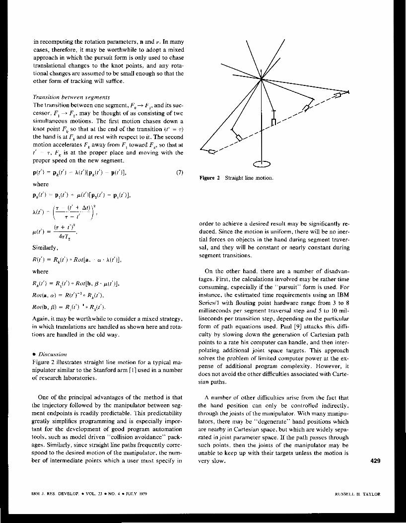
Discussion Figure 2 illustrates straight line motion for a typical manipulator similar to the Stanford arm [ l] used in a number of research laboratories.

One of the principal advantages of the method is that the trajectory followed by the manipulator between segment endpoints is readily predictable. This predictability greatly simplifies programming and is especially important for the development of good program automation tools, such as model driven “collision avoidance” pack- ages. Similarly, since straight line paths frequently correspond to the desired motion of the manipulator, the number of intermediate points which a user must specify in

C

k

Figure 2 Straight line motion.

order to achieve a desired result may be significantly reduced. Since the motion is uniform, there will be no inertial forces on objects in the hand during segment traversal, and they will be constant or nearly constant during segment transitions.

On the other hand, there are a number of disadvantages. First, the calculations involved may be rather time consuming, especially if the “pursuit” form is used. For instance, the estimated time requirements using an IBM Series11 with floating point hardware range from 3 to 8 milliseconds per segment traversal step and 5 to 10 milliseconds per transition step, depending on the particular form of path equations used. Paul [ 9 ] attacks this difficulty by slowing down the generation of Cartesian path points to a rate his computer can handle, and then inter- polating additional joint space targets. This approach solves the problem of limited computer power at the expense of additional program complexity. However, it does not avoid the other difficulties associated with Carte- sian paths.

A number of other difficulties arise from the fact that the hand position can only be controlled indirectly, through the joints of the manipulator. With many manipulators, there may be “degenerate” hand positions which are nearby in Cartesian space, but which are widely sepa- rated in joint parameter space. If the path passes through such points, then the joints of the manipulator may be unable to keep up with their targets unless the motion is very slow. 429


This problem may be solved at the expense of additional computation and programming complexity by using the current joint velocities to recompute at each sample interval how large a fraction, h( t + At) - h ( t ) , of the segment is to be covered in the next sample interval [9]. The path followed will still be a straight line, but the hand will not move at uniform speed, so that objects in the hand will experience various inertial forces, which will be difficult to predict without “simulating” the motion in advance. Also, coordinated motions involving several manipulators are more difficult to plan, since it is difficult to predict just where each manipulator will be at a given time.

Physical stops or limits on individual joints of the manipulator introduce complications similar to those introduced by degenerate axis alignments. In order to move the hand to a nearby point, it may be necessary to “un- wind” a joint through 359” rather than advance it through 1”. Such discontinuities cannot be handled well unless they have been anticipated. Simple schemes which merely adjust speeds based on joint velocities cannot do this.

Finally, the fact that there are generally several possible sets of joint parameters which can place the hand at a desired target frame F( t ) introduces still further complications. Unless a certain amount of care is taken in the joint solution procedure, discontinuities in the joint target values may be introduced at awkward moments. Indeed, it may frequently be very important to select the solution which minimizes the total motion required through a many segment motion, or to avoid a joint stop during a critical segment. It is unclear just how this can be done without a certain amount of preplanning which pays at- tention to joint space trajectories.

The conclusion is that, although Cartesian path interpolation offers a number of significant advantages, the joint space behavior of the manipulator itself cannot be ignored. The joint space strategy described in the next section preserves many of the advantages of Cartesian path control, while requiring somewhat lower computational effort and allowing joint space considerations to be handled more easily.

Bounded deviation joint paths The principal disadvantages of Cartesian path control are the amount of real time computation required and the difficulty of dealing in real time with constraints on the joint space behavior of the manipulator. These problems may be avoided or at least greatly reduced by preplanning the motion before it is executed. Sometimes this preplanning

430 can be performed well in advance. Often, however, the

values of the knot points are not known until just before the motion is executed. In such cases, it is important that the time the manipulator spends waiting for planning to be completed be kept as short as possible.

As an extreme case, the real time algorithm could be simulated and used to precompute the joint parameters for every sample interval. Motion execution would then be trivial: the joint parameter values would simply be read from memory and used as local goals for the servoing algorithm. Such a policy, however, is rather wasteful, since the amount of data that would have to be stored is quite large and since the computation time needed may approach that required by the motion itself.

One possible way out would be to precompute the joint solutions for every nth sample interval and then to per- form interpolation on the joint parameters to generate real time goals. The difficulty with this method is that the number of intermediate points needed to keep the manipulator acceptably close to a straight Cartesian path de- pends on the particular motion being made. Any “stan- dard” interval small enough to guarantee low deviations everywhere will require a wasteful amount of pre- computation for many motions.

This section presents a simple algorithm which generates only enough intermediate points to guarantee that the manipulator’s deviation from a straight path on each motion segment stays within prespecified error bounds.

Joint spuce motion strategy Suppose we compute joint parameter vectors j , corresponding to the knot points F, of our desired motion. We can then use these j , as the knot points for a joint space interpolation strategy analogous to that used for the position part of our Cartesian space paths. For motion from j , to j,, we have

j ( t ) = j , - ~

T , - t T . A j , ,

I

and for transition between j , -+ j , and j , + j , ,

(7 - t ’ ) , (7 + t y j ( t ‘ ) = j , - ___ 47 T , A j , + 47 T, Aj , ,

where Aj , = j , - j , , , A j , = j , - j , , and T, , T,, T , and t’ have the same meanings as for the Cartesian path motion. Here, the joints of the manipulator move at uniform velocity between the knot points and make smooth transitions with constant acceleration between segments [15].

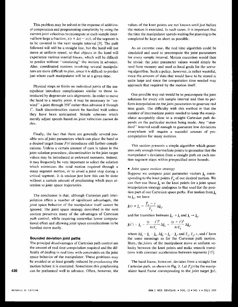
The hand frame, however, deviates from a straight line Cartesian path, as shown in Fig. 3 . Let Fj( t ) be the manipulator hand frame corresponding to the joint target j ( t ) ,


70

-

- 50 -

- 40 -

-

30 - motion

- Recursion h i t = 0 0 I 1 I I I I I I I

- % -3 0.4 - 8 Recursion limit = 2

I I I I I I I I I 0.4

Figure 3 X coordinate of hand for (t3y = 0.5 cm, SEaX = 5").

0.6

typical motion

0.8

segment, with

and let F,(t) be the frame target for the corresponding Cartesian space path. Then, the displacement deviation S,(t) and the rotation deviation 8 J t ) are defined as

a p ( f ) = IP,(t) - P,(t)l,

8,(r) = [angle part of R,(r)-' 0 R,(t)l.

Point interpolation method Consider an arbitrary motion segment, F, + F , , for which we have specified the maximum acceptable deviations:

IBM J. RES. DEVELOP. VOL. 23 NO. 4 JULY 1

Rccurslon limit = I I I I I I I I I

- -

Recursion limit = 3 I I I I I I I I I

0.0

midpoint

0.2

interpolation

0.4 0.6 0.8

limited to 0, 1 , 2, and 3 levels of

1.0

' recursion

We must specify enough intermediate points along the Cartesian path so that the path deviations introduced by straight line interpolation between the corresponding joint solutions stay within these bounds. The generation of an "optimal" set of intermediate points requires a good characterization of the path deviation functions 8:" and 8yX. These functions depend on the particular manipulator being used and can be quite complicated. For many 431

RUSSELL n. TAYLOR 979

0.2 0.4 0.6 0.8 1.0

I Normalized time

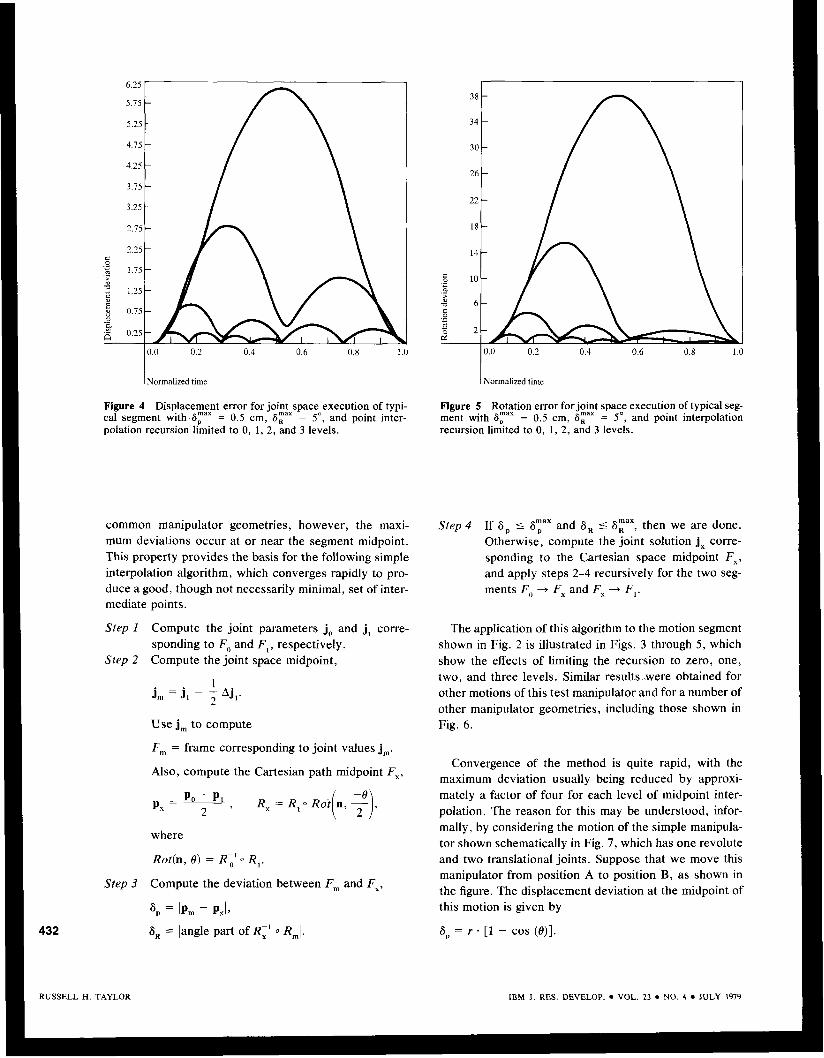
Figure 4 Displacement error for joint space execution of typical segment with 8 r = 0.5 cm, ,Fax = 5", and point interpolation recursion limited to 0, 1 , 2 , and 3 levels.

common manipulator geometries, however, the maximum deviations occur at or near the segment midpoint. This property provides the basis for the following simple interpolation algorithm, which converges rapidly to produce a good, though not necessarily minimal, set of intermediate points.

Step 1 Compute the joint parameters j, and j, corre-

Srep 2 Compute the joint space midpoint, sponding to F,, and F,, respectively.

I jm = j, - ; A j l .

i

Use j, to compute

F, = frame corresponding to joint values j,.

Also, compute the Cartesian path midpoint F,,

P, = + 2 ' Rx = R,o Ruijn, $1,

432

RUSSELL H. TAYLOR

where

Rot(n, 6 ) = Ri'o R,.

Step 3 Compute the deviation between F, and Fx,

fjD = IP, - PXL

6, = langle part of R,' 0 R,I.

I Normalized time

Figure 5 Rotation error for joint space execution of typical segment with 8 r = 0.5 cm, 8;'' = So, and point interpolation recursion limited to 0, 1 , 2 , and 3 levels.

Step 4 If 6, 5 and 8, 6rx, then we are done. Otherwise, compute the joint solution jx corresponding to the Cartesian space midpoint F,, and apply steps 2-4 recursively for the two segments F, + F, and F, -+ F,.

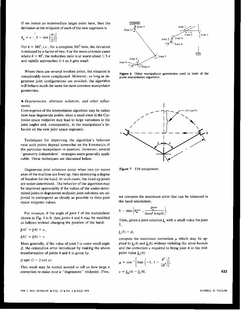
The application of this algorithm to the motion segment shown in Fig. 2 is illustrated in Figs. 3 through 5, which show the effects of limiting the recursion to zero, one, two, and three levels. Similar results ,were obtained for other motions of this test manipulator and for a number of other manipulator geometries, including those shown in Fig. 6.

Convergence of the method is quite rapid, with the maximum deviation usually being reduced by approximately a factor of four for each level of midpoint interpolation. The reason for this may be understood, infor- mally, by considering the motion of the simple manipulator shown schematically in Fig. 7, which has one revolute and two translational joints. Suppose that we move this manipulator from position A to position B, as shown in the figure. The displacement deviation at the midpoint of this motion is given by

6, = r . [I - cos (8 ) ] .

IBM I. RES. DEVELOP. VOL. 23 a NO. 4 JULY 1979

If we invent an intermediate target point here, then the deviation at the midpoint of each of the new segments is

For I9 = ISO”, i . e . , for a complete 360” turn, the deviation is reduced by a factor of two. For the more common cases where I9 5 90°, the reduction ratio is at worst about 1 : 3.4 and rapidly approaches 1 : 4 as I9 gets small.

Where there are several revolute joints, the situation is considerably more complicated. However, so long as degenerate joint configurations are avoided, the algorithm will behave much the same for most common manipulator geometries.

Degeneracies, alternate solutions, and other refine- ments Convergence of the interpolation algorithm may be rather slow near degenerate points, since a small error in the Car- tesian space midpoint may lead to large variations in the joint angles and, consequently, in the manipulator’s behavior on the new joint space segments.

Techniques for improving the algorithm’s behavior near such points depend somewhat on the kinematics of the particular manipulator in question. However, several “geometry independent” strategies seem generally appli- cable. These techniques are discussed below.

Degenerate joint solutions occur when two (or more) axes of the machine are lined up, thus destroying a degree of freedom for the hand. In such cases, the lined-up joints are under-determined. The behavior of the algorithm may be improved appreciably if the values of the under-determined joints in degenerate midpoint joint solutions are ad- justed to correspond as closely as possible to their joint space midpoint values.

For instance, if the angle of joint 5 of the manipulator shown in Fig. 1 is 0, then joints 4 and 6 may be modified as follows without changing the position of the hand:

j(4)‘ = j(4) + v, j(6)’ = j(6) - v.

More generally, if the value of joint 5 is some small angle p, the orientation error introduced by making the above transformation of joints 4 and 6 is given by

p sqrt ( 2 - 2 cos v).

This result may be turned around to tell us how large a correction to make near a “degenerate” midpoint. First,

Joint 2

Joint 6

Joint 6

Bi

- I Joint 1

%

Figure 6 Other manipulator geometries used in tests of the point interpolation algorithm.

Figure 7 XYB manipulator.

we compute the maximum error that can be tolerated in the hand orientation:

6 = min 6pX ,

Then, given a joint solution jx with a small value for joint 5 ,

jx(5) =

( hand length 1. Y a X

compute the maximum correction p which may be applied to jx(4) and jx(6) without violating the error bounds and the correction v required to bring joint 4 to the midpoint value jm(4):

p = COS-l[nlax (-1, 1 - -j], 62

2P2

433

1. TAYLOR IBM J. RES. DEVELOP. 1 IOL. 2 3 NO. 4 JULY 1979 RUSSELL 1

434

2.8

0.0 0.2 0.4 0.6 0.8 1

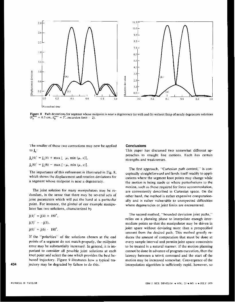
Figure 8 Path deviations for segment whose midpoint is near a degeneracy (a) with and (b) without fixup of nearly degenerate solutions (8y = 0.5 cm, = 5”, recursion limit = 2).

The smaller of these two corrections may now be applied to jx:

jx(4)’ = jx(4) + max [ -p , min (p, v)l,

jx(6)’ = jx(6) - max [ -p , min (p, v)].

The importance of this refinement is illustrated in Fig. 8, which shows the displacement and rotation deviations for a segment whose midpoint is near a degeneracy.

The joint solution for many manipulators may be redundant, in the sense that there may be several sets of joint parameters which will put the hand at a particular point. For instance, the gimbal of our example manipulator has two solutions, characterized by

j(4)‘ = j(4) + 180”,

j (9’ = -j(5),

j(6)’ = j(6) - 180”.

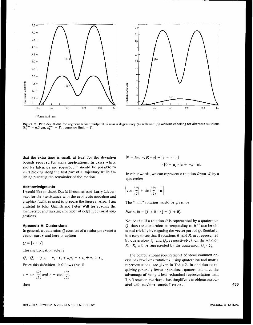
If the “polarities” of the solutions chosen at the end points of a segment do not match properly, the midpoint error may be substantially increased. In general, it is important to consider all possible joint solutions at each knot point and select the one which provides the best be- haved trajectory. Figure 9 illustrates how a typical trajectory may be degraded by failure to do this.

Conclusions This paper has discussed two somewhat different approaches to straight line motions. Each has certain strengths and weaknesses.

The first approach, “Cartesian path control,” is conceptually straightforward and lends itself readily to applications where the segment knot points may change while the motion is being made or where perturbations to the motion, such as those required for force accommodation, are conveniently described in Cartesian space. On the other hand, the method is rather expensive computation- ally and is rather vulnerable to unexpected difficulties where degeneracies or joint limits are encountered.

The second method, “bounded deviation joint paths,” relies on a planning phase to interpolate enough intermediate points so that the manipulator may be driven in joint space without deviating more than a prespecified amount from the desired path. This method greatly reduces the amount of computation that must be done at every sample interval and permits joint space constraints to be treated in a natural manner. If the motion planning cannot be done in advance of program execution, then the latency between a MOVE command and the start of the motion may be increased somewhat. Convergence of the interpolation algorithm is sufficiently rapid, however, so


0.0 0.2 0.4 0.6 0.8

I Normalized time

Figure 9 Path deviations for segment whose midpoint is near a degeneracy (a) with and (b) without checking for alternate solutions (a? = 0.5 cm, By = 5", recursion limit = 1) .

that the extra time is small, at least for the deviation bounds required for many applications. In cases where shorter latencies are required, it should be possible to start moving along the first part of a trajectory while fin- ishing planning the remainder of the motion.

Acknowledgments 1 would like to thank David Grossman and Larry Lieber- man for their assistance with the geometric modeling and graphics facilities used to prepare the figures. Also, I am grateful to John Griffith and Peter Will for reading the manuscript and making a number of helpful editorial sug- gestions.

Appendix A: Quaternions In general, a quaternion Q consists of a scalar part s and a vector part v and here is written

Q = [s + v].

The multiplication rule is

Q 1 o Q, = [ s , s ~ - v1 . v2 + S , V ~ + s l V z + V I X vz].

From this definition, it follows that if

s = sin 1;) and c = cos ( 3 ,

then

[0 + Rot(n, 0) 0 u] = [c + s . n]

0 [O + u] 0 [ c + --s . n].

In other words, we can represent a rotation Rot(n, 0) by a quaternion

The "null" rotation would be given by

Rot(n, 0) = [ I + 0 . n] = [l + 01.

Notice that if a rotation R is represented by a quaternion Q , then the quaternion corresponding to R" can be obtained trivially by negating the vector part of Q. Similarly, it is easy to see that if rotations R, and R, are represented by quaternions Q, and Q2, respectively, then the rotation R, 0 R, will be represented by the quaternion Q, 0 Q,.

The computational requirements of some common operations involving rotations, using quaternion and matrix representations, are given in Table 2 . In addition to requiring generally fewer operations, quaternions have the advantage of being a less redundant representation than 3 X 3 rotation matrices, thus simplifying problems associated with machine roundoff errors. 435

RUSSELL H. TAYLOR IBM J . RES, DEVELOP. VOL. 23 NO. 4 JULY 1979

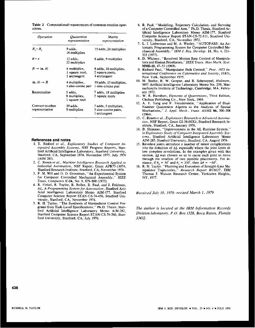
Table 2 Computational requirements of common rotation oper- 6. R. Paul, “Modelling, Trajectory Calculation, and Servoing ations. of a Computer Controlled Arm,” Ph.D. Thesis, Stanford Ar-

tificial Intelligence Laboratory Memo AIM-177, Stanford Operation Quaternion Matrix Computer Science Report STAN-CS-72-3 11, Stanford Uni-

representation representation versity, Stanford, CA, November 1972. 7. L. I . Lieberman and M. A. Wesley, “AUTOPASS: An Au-

tomatic Programming System for Computer Controlled Me- chanical Assembly,” ZBM J . Res. Develop. 21, No. 4, 321- 333 (1977).

R, R, 9 adds, 15 adds, 24 multiplies 16 multiplies

R o u 12 adds, 6 adds, 9 multiplies 22 multiplies

R + (n, 8) 4 multiplies, 8 adds, 10 multiplies, 1 square root, 2 square roots, 1 arctangent 1 arctangent

(n, 8 ) + R 4 multiplies, 10 adds, 15 multiplies, 1 sine-cosine pair 1 sine-cosine pair

Renormalize 3 adds, 7 adds, 18 multiplies 8 multiplies, 2 square roots 1 square root

Convert to other 19 adds, representation

7 adds, 5 multiplies, 9 multiplies 3 sine-cosine pairs,

1 arctangent

References and notes 1. T. Binford et al . , Exploratory Studies of Computer In-

tegrated Assembly Systems, NSF Progress Reports, Stan- ford Artificial Intelligence Laboratory, Stanford University, Stanford, CA, September 1974, November 1975, July 1976 (AIM 285).

2. C. Rosen et al., Machine Intelligence Research Applied to Industrial Automation, NSF Report, Grant APR75-13074, Stanford Research Institute, Stanford, CA, November 1976.

3. P. M. Will and D. D. Grossman, “An Experimental System for Computer Controlled Mechanical Assembly,” ZEEE Trans. Computers (2-24, No. 9, 879-888 (1975).

4. R. Finkel, R. Taylor, R. Bolles, R. Paul, and J. Feldman, AL, A Programming System for Automation, Stanford Arti- ficial Intelligence Laboratory Memo AIM-177, Stanford Computer Science Report STAN-(3-74-456, Stanford Uni- versity, Stanford, CA, November 1974.

5 . R. H. Taylor, “The Synthesis of Manipulator Control Pro- grams from Task-Level Specifications,” Ph.D. Thesis, Stan- ford Artificial Intelligence Laboratory Memo AIM-282, Stanford Computer Science Report STAN-CS-76-560, Stan- ford University, Stanford, CA, July 1976.

8. D. Whitney, “pesolved Motion Rate Control of Manipula- tors and Human Prostheses,”ZEEE Trans. Man Mach. Syst.

9. Richard Paul, “Manipulator Path Control,” Proc. 1975 Zn- ternational Conference on Cybernetics and Society, IEEE, New York, September 1975.

10. M. Beeler, R. W. Gosper, and R. Schroeppel, Hakmem, MIT Artificial Intelligence Laboratory Memo No. 239, Mas- sachusetts Institute of Technology, Cambridge, MA, Febru- ary 1972.

11. W. R. Hamilton, Elements of Quaternions, Third Edition, Chelsea Publishing Co., New York, 1969.

12. A. T. Yang and F. Freudenstein, “Application of Dual- Number Quaternion Algebra to the Analysis of Spatial Mechanisms,” J . Appl. Mech., Trans. ASME 86, 300-308 (1964).

13. C. Rosen et al., Exploratory Research in Advanced Automa- tion, NSF Report, Grant GI-38100x1, Stanford Research In- stitute, Stanford, CA, January 1976.

14. B. Shimano, “Improvements in the AL Runtime System,” in Exploratory Study of Computer.lntegrated Assembly Sys- tems, Stanford Artificial Intelligence Laboratory Memo AIM-285, Stanford University, Stanford, CA, August 1976.

15. Revolute joints introduce a number of minor complications into the definition of Aj, especially where the joint limits allow complete revolutions. In the examples given with this section, A j was chosen so as to cause each joint to move through the smallest of two possible placements. For instance, if Bo = 30” and 8, = 330°, then A8 = -60”.

16. R. H. Taylor, “Planning and Execution of Straight-Line Ma- nipulator Trajectories,” Research Report RC6657, IBM Thomas J. Watson Research Center, Yorktown Heights, NY, 1977.

“S-IO, 47-53 (1969).

Received July 10, 1978; revised March 1 , 1979

The author is located at the IBM Information Records Division laboratory, P.O. Box 1328, Boca Raton, Florida 33432.

436


planning and execution of straight line manipulator ...rht/rht papers/1979/straight line...

Documents