planning and acting in partially observable...

Artificial Intelligence 101 (1998) 99–134

Planning and acting in partially observablestochastic domains

Leslie Pack Kaelblinga,∗,1,2, Michael L. Littmanb,3,Anthony R. Cassandrac,1

a Computer Science Department, Brown University, Box 1910, Providence, RI 02912-1910, USAb Department of Computer Science, Duke University, Durham, NC 27708-0129, USA

c Microelectronics and Computer Technology Corporation (MCC), 3500 West Balcones Center Drive, Austin,TX 78759-5398, USA

Received 11 October 1995; received in revised form 17 January 1998

Abstract

In this paper, we bring techniques from operations research to bear on the problem of choosingoptimal actions in partially observable stochastic domains. We begin by introducing the theoryof Markov decision processes (MDPs) and partially observableMDPs (POMDPs). We then outlinea novel algorithm for solvingPOMDPs off line and show how, in some cases, a finite-memorycontroller can be extracted from the solution to aPOMDP. We conclude with a discussion of how ourapproach relates to previous work, the complexity of finding exact solutions toPOMDPs, and of somepossibilities for finding approximate solutions. 1998 Elsevier Science B.V. All rights reserved.

Keywords:Planning; Uncertainty; Partially observable Markov decision processes

Consider the problem of a robot navigating in a large office building. The robot can movefrom hallway intersection to intersection and can make local observations of its world.Its actions are not completely reliable, however. Sometimes, when it intends to move, itstays where it is or goes too far; sometimes, when it intends to turn, it overshoots. It hassimilar problems with observation. Sometimes a corridor looks like a corner; sometimes aT-junction looks like an L-junction. How can such an error-plagued robot navigate, evengiven a map of the corridors?

∗ Corresponding author. Email: [email protected] Supported in part by NSF grants IRI-9453383 and IRI-9312395.2 Supported in part by DARPA/Rome Labs Planning Initiative grant F30602-95-1-0020.3 Supported in part by Bellcore and NSF CAREER grant IRI-9702576.

0004-3702/98/$19.00 1998 Elsevier Science B.V. All rights reserved.PII: S0004-3702(98)00023-X

100 L.P. Kaelbling et al. / Artificial Intelligence 101 (1998) 99–134

In general, the robot will have to remember something about its history of actionsand observations and use this information, together with its knowledge of the underlyingdynamics of the world (the map and other information), to maintain an estimate of itslocation. Many engineering applications follow this approach, using methods like theKalman filter [26] to maintain a running estimate of the robot’s spatial uncertainty,expressed as an ellipsoid or normal distribution in Cartesian space. This approach willnot do for our robot, though. Its uncertainty may be discrete: it might be almost certain thatit is in the north-east corner of either the fourth or the seventh floors, though it admits achance that it is on the fifth floor, as well.

Then, given an uncertain estimate of its location, the robot has to decide what actionsto take. In some cases, it might be sufficient to ignore its uncertainty and take actions thatwould be appropriate for the most likely location. In other cases, it might be better forthe robot to take actions for the purpose of gathering information, such as searching fora landmark or reading signs on the wall. In general, it will take actions that fulfill bothpurposes simultaneously.

1. Introduction

In this paper, we bring techniques from operations research to bear on the problem ofchoosing optimal actions in partially observable stochastic domains. Problems like theone described above can be modeled aspartially observable Markov decision processes(POMDPs). Of course, we are not interested only in problems of robot navigation. Similarproblems come up in factory process control, oil exploration, transportation logistics, anda variety of other complex real-world situations.

This is essentially aplanning problem: given a complete and correct model of theworld dynamics and a reward structure, find an optimal way to behave. In the artificialintelligence (AI) literature, a deterministic version of this problem has been addressedby adding knowledge preconditions to traditional planning systems [43]. Because weare interested in stochastic domains, however, we must depart from the traditional AIplanning model. Rather than taking plans to be sequences of actions, which may onlyrarely execute as expected, we take them to be mappings from situations to actions thatspecify the agent’s behavior no matter what may happen. In many cases, we may not wanta full policy; methods for developing partial policies and conditional plans for completelyobservable domains are the subject of much current interest [13,15,61]. A weakness of themethods described in this paper is that they require the states of the world to be representedenumeratively, rather than through compositional representations such as Bayes nets orprobabilistic operator descriptions. However, this work has served as a substrate fordevelopment of algorithms for more complex and efficient representations [6]. Section 6describes the relation between the present approach and prior research in more detail.

One important facet of thePOMDPapproach is that there is no distinction drawn betweenactions taken to change the state of the world and actions taken to gain information. Thisis important because, in general, every action has both types of effect. Stopping to askquestions may delay the robot’s arrival at the goal or spend extra energy; moving forwardmay give the robot information that it is in a dead-end because of the resulting crash.

L.P. Kaelbling et al. / Artificial Intelligence 101 (1998) 99–134 101

Thus, from thePOMDP perspective, optimal performance involves something akin to a“value of information” calculation, only more complex; the agent chooses between actionsbased on the amount of information they provide, the amount of reward they produce, andhow they change the state of the world.

This paper is intended to make two contributions. The first is to recapitulate work fromthe operations-research literature [36,42,56,59,64]and to describe its connection to closelyrelated work in AI. The second is to describe a novel algorithmic approach for solvingPOMDPs exactly. We begin by introducing the theory of Markov decision processes (MDPs)andPOMDPs. We then outline a novel algorithm for solvingPOMDPs off line and show how,in some cases, a finite-memory controller can be extracted from the solution to aPOMDP.We conclude with a brief discussion of related work and of approximation methods.

2. Markov decision processes

Markov decision processes serve as a basis for solving the more complex partiallyobservable problems that we are ultimately interested in. AnMDP is a model of an agentinteracting synchronously with a world. As shown in Fig. 1, the agent takes as input thestate of the world and generates as output actions, which themselves affect the state of theworld. In theMDP framework, it is assumed that, although there may be a great deal ofuncertainty about the effects of an agent’s actions, there is never any uncertainty about theagent’s current state—it has complete and perfect perceptual abilities.

Markov decision processes are described in depth in a variety of texts [3,49]; we willjust briefly cover the necessary background.

2.1. Basic framework

A Markov decision process can be described as a tuple〈S,A, T ,R〉, where• S is a finite set of states of the world;• A is a finite set of actions;• T :S ×A→Π(S) is thestate-transition function, giving for each world state and

agent action, a probability distribution over world states (we writeT (s, a, s′) forthe probability of ending in states′, given that the agent starts in states and takesactiona); and

Fig. 1. AnMDP models the synchronous interaction between agent and world.


• R :S ×A→R is the reward function, giving the expected immediate reward gainedby the agent for taking each action in each state (we writeR(s, a) for the expectedreward for taking actiona in states).

In this model, the next state and the expected reward depend only on the previous stateand the action taken; even if we were to condition on additional previous states, thetransition probabilities and the expected rewards would remain the same. This is knownas theMarkovproperty—the state and reward at timet + 1 is dependent only on the stateat timet and the action at timet .

In fact, MDPs can have infinite state and action spaces. The algorithms that we describein this section apply only to the finite case; however, in the context ofPOMDPs, we willconsider a class ofMDPs with uncountably infinite state spaces.

2.2. Acting optimally

We would like our agents to act in such a way as to maximize some measure of thelong-run reward received. One such framework isfinite-horizonoptimality, in which theagent should act in order to maximize the expected sum of reward that it gets on the nextk

steps; it should maximize

E

[k−1∑t=0

rt

]wherert is the reward received on stept . This model is somewhat inconvenient, because itis rare that an appropriatek will be known exactly. We might prefer to consider an infinitelifetime for the agent. The most straightforward is theinfinite-horizon discountedmodel,in which we sum the rewards over the infinite lifetime of the agent, but discount themgeometrically usingdiscount factor0< γ < 1; the agent should act so as to optimize

E

[ ∞∑t=0

γ t rt

].

In this model, rewards received earlier in its lifetime have more value to the agent; theinfinite lifetime is considered, but the discount factor ensures that the sum is finite. Thissum is also the expected amount of reward received if a decision to terminate the runis made on each step with probability 1− γ . The larger the discount factor (closer to1), the more effect future rewards have on current decision making. In our forthcomingdiscussions of finite-horizon optimality, we will also use a discount factor; when it hasvalue one, it is equivalent to the simple finite-horizon case described above.

A policy is a description of the behavior of an agent. We consider two kinds of policies:stationary and nonstationary. Astationary policy, π :S→A, is a situation-action mappingthat specifies, for each state, an action to be taken. The choice of action depends only on thestate and is independent of the time step. Anonstationary policyis a sequence of situation-action mappings, indexed by time. The policyπt is to be used to choose the action on thet th-to-last step as a function of the current state,st . In the finite-horizon model, the optimalpolicy is not typically stationary: the way an agent chooses its actions on the last step of itslife is generally going to be very different from the way it chooses them when it has a long


life ahead of it. In the infinite-horizon discounted model, the agent always has a constantexpected amount of time remaining, so there is no reason to change action strategies: thereis a stationary optimal policy.

Given a policy, we can evaluate it based on the long-run value that the agent expects togain from executing it. In the finite-horizon case, letVπ,t (s) be the expected sum of rewardgained from starting in states and executing nonstationary policyπ for t steps. Clearly,Vπ,1(s) = R(s,π1(s)); that is, on the last step, the value is just the expected reward fortaking the action specified by the final element of the policy. Now, we can defineVπ,t (s)

inductively as

Vπ,t (s)=R(s,πt (s)

)+ γ ∑s ′∈S

T(s,πt (s), s

′)Vπ,t−1(s′).

Thet-step value of being in states and executing nonstationary policyπ is the immediatereward,R(s,πt (s)), plus the discounted expected value of the remainingt − 1 steps. Toevaluate the future, we must consider all possible resulting statess′, the likelihood of theiroccurrenceT (s,πt (s), s′), and their(t − 1)-step value under policyπ , Vπ,t−1(s

′). In theinfinite-horizon discounted case, we writeVπ(s) for the expected discounted sum of futurereward for starting in states and executing policyπ . It is recursively defined by

Vπ(s)=R(s,π(s)

)+ γ ∑s ′∈S

T(s,π(s), s′

)Vπ(s′).

The value function,Vπ , for policyπ is the unique simultaneous solution of this set of linearequations, one equation for each states.

Now we know how to compute a value function, given a policy. Sometimes, we willneed to go the opposite way, and compute agreedy policygiven a value function. It reallyonly makes sense to do this for the infinite-horizon discounted case; to derive a policy forthe finite horizon, we would need a whole sequence of value functions. Given any valuefunctionV , a greedy policy with respect to that value function,πV , is defined as

πV (s)= argmaxa

[R(s, a)+ γ

∑s ′∈S

T(s, a, s′

)V(s′)].

This is the policy obtained by, at every step, taking the action that maximizes expectedimmediate reward plus the expected discounted value of the next state, as measured byV .

What is the optimal finite-horizon policy,π∗? The agent’s last step is easy: it shouldmaximize its final reward. So

π∗1 (s)= argmaxa

R(s, a).

The optimal situation-action mapping for thet th step,π∗t , can be defined in terms of theoptimal(t − 1)-step value functionVπ∗t−1,t−1 (written for simplicity asV ∗t−1):

π∗t (s)= argmaxa

[R(s, a)+ γ

∑s ′∈S

T(s, a, s′

)V ∗t−1

(s′)];

V ∗t−1 is derived fromπ∗t−1 andV ∗t−2.


In the infinite-horizon discounted case, for any initial states, we want to execute thepolicy π that maximizesVπ(s). Howard [24] showed that there exists a stationary policy,π∗, that is optimal for every starting state. The value function for this policy,Vπ∗ , alsowrittenV ∗, is defined by the set of equations

V ∗(s)=maxa

[R(s, a)+ γ

∑s ′∈S

T(s, a, s′

)V ∗(s′)],

which has a unique solution. An optimal policy,π∗, is just a greedy policy with respectto V ∗.

Another way to understand the infinite-horizon value function,V ∗, is to approach it byusing an ever-increasing discounted finite horizon. As the horizon,t , approaches infinity,V ∗t approachesV ∗. This is only guaranteed to occur when the discount factor,γ , is lessthan 1, which tends to wash out the details of exactly what happens at the end of the agent’slife.

2.3. Computing an optimal policy

There are many methods for finding optimal policies forMDPs. In this section, weexplorevalue iterationbecause it will also serve as the basis for finding policies in thepartially observable case.

Algorithm 1. The value-iteration algorithm for finite state spaceMDPs.

V1(s) := 0 for all st := 1loop

t := t + 1loop for all s ∈ S

loop for all a ∈AQat (s) :=R(s, a)+ γ

∑s ′∈S T (s, a, s′)Vt−1(s

′)end loop

Vt(s) :=maxa Qat (s)end loop

until |Vt(s)−Vt−1(s)|< ε for all s ∈ S

Value iteration proceeds by computing the sequenceVt of discounted finite-horizonoptimal value functions, as shown in Algorithm 1 (the superscript∗ is omitted, because weshall henceforth only be considering optimal value functions). It makes use of an auxiliaryfunction,Qat (s), which is thet-step value of starting in states, taking actiona, thencontinuing with the optimal(t − 1)-step nonstationary policy. The algorithm terminateswhen the maximum difference between two successive value functions (known as theBellman error magnitude) is less than someε. It can be shown [62] that there exists at∗,polynomial in|S|, |A|, the magnitude of the largest value ofR(s, a), and 1/(1− γ ), suchthat the greedy policy with respect toVt∗ is equal to the optimal infinite-horizon policy,π∗.Rather than calculating a bound ont∗ in advance and running value iteration for that long,


we instead use the following result regarding the Bellman error magnitude [66] in order toterminate with a near-optimal policy.

If |Vt(s)− Vt−1(s)|< ε for all s, then the value of the greedy policy with respect toVtdoes not differ fromV ∗ by more than 2εγ /(1− γ ) at any state. That is,

maxs∈S

∣∣VπVt (s)− V ∗(s)∣∣< 2εγ

1− γ .It is often the case thatπVt = π∗ long beforeVt is nearV ∗; tighter bounds may be obtainedusing thespan semi-normon the value function [49].

3. Partial observability

For MDPs we can compute the optimal policyπ and use it to act by simply executingπ(s) for current states. What happens if the agent is no longer able to determine the stateit is currently in with complete reliability? A naive approach would be for the agent to mapthe most recent observation directly into an action without remembering anything from thepast. In our hallway navigation example, this amounts to performing the same action inevery location that looks the same—hardly a promising approach. Somewhat better resultscan be obtained by adding randomness to the agent’s behavior: a policy can be a mappingfrom observations to probability distributions over actions [55]. Randomness effectivelyallows the agent to sometimes choose different actions in different locations with thesame appearance, increasing the probability that it might choose a good action; in practicedeterministic observation-action mappings are prone to getting trapped in deterministicloops [32].

In order to behave truly effectively in a partially observable world, it is necessary to usememory of previous actions and observations to aid in the disambiguation of the states ofthe world. ThePOMDPframework provides a systematic method of doing just that.

3.1. POMDP framework

A partially observable Markov decision process can be described as a tuple〈S,A, T ,R,Ω,O〉, where• S,A, T , andR describe a Markov decision process;• Ω is a finite set of observations the agent can experience of its world; and• O :S × A → Π(Ω) is the observation function, which gives, for each action

and resulting state, a probability distribution over possible observations (we writeO(s′, a, o) for the probability of making observationo given that the agent took actiona and landed in states′).

A POMDPis anMDP in which the agent is unable to observe the current state. Instead, itmakes an observation based on the action and resulting state.4 The agent’s goal remainsto maximize expected discounted future reward.

4 It is possible to formulate an equivalent model in which the observation depends on the previous state insteadof, or in addition to, the resulting state, but it complicates the exposition and adds no more expressive power; sucha model could be converted into aPOMDPmodel as described above, at the cost of expanding the state space.


Fig. 2. A POMDPagent can be decomposed into a state estimator (SE) and a policy (π ).

3.2. Problem structure

We decompose the problem of controlling aPOMDP into two parts, as shown in Fig. 2.The agent makes observations and generates actions. It keeps an internalbelief state, b, thatsummarizes its previous experience. The component labeled SE is thestate estimator: it isresponsible for updating the belief state based on the last action, the current observation,and the previous belief state. The component labeledπ is the policy: as before, it isresponsible for generating actions, but this time as a function of the agent’s belief staterather than the state of the world.

What, exactly, is a belief state? One choice might be the most probable state of theworld, given the past experience. Although this might be a plausible basis for action insome cases, it is not sufficient in general. In order to act effectively, an agent must takeinto account its own degree of uncertainty. If it is lost or confused, it might be appropriatefor it to take sensing actions such as asking for directions, reading a map, or searching fora landmark. In thePOMDP framework, such actions are not explicitly distinguished: theirinformational properties are described via the observation function.

Our choice for belief states will be probability distributions over states of the world.These distributions encode the agent’s subjective probability about the state of the worldand provide a basis for acting under uncertainty. Furthermore, they comprise asufficientstatistic for the past history and initial belief state of the agent: given the agent’s currentbelief state (properly computed), no additional data about its past actions or observationswould supply any further information about the current state of the world [1,56]. Thismeans that the process over belief states is Markov, and that no additional data about thepast would help to increase the agent’s expected reward.

To illustrate the evolution of a belief state, we will use the simple example depicted inFig. 3; the algorithm for computing belief states is provided in the next section. There arefour states in this example, one of which is a goal state, indicated by the star. There aretwo possible observations: one is always made when the agent is in state 1, 2, or 4; theother, when it is in the goal state. There are two possible actions:EAST andWEST. Theseactions succeed with probability 0.9, and when they fail, the movement is in the opposite


Fig. 3. In this simplePOMDP environment, the empty squares are all indistinguishable on the basis of theirimmediate appearance, but the evolution of the belief state can be used to model the agent’s location.

direction. If no movement is possible in a particular direction, then the agent remains inthe same location.

Assume that the agent is initially equally likely to be in any of the three nongoal states.Thus, its initial belief state is[0.333 0.333 0.000 0.333], where the position in thebelief vector corresponds to the state number.

If the agent takes actionEAST and does not observe the goal, then the new belief statebecomes[0.100 0.450 0.000 0.450]. If it takes actionEAST again, and still does notobserve the goal, then the probability mass becomes concentrated in the right-most state:[0.100 0.164 0.000 0.736]. Notice that as long as the agent does not observe the goalstate, it will always have some nonzero belief that it is in any of the nongoal states, sincethe actions have nonzero probability of failing.

3.3. Computing belief states

A belief stateb is a probability distribution overS. We letb(s) denote the probabilityassigned to world states by belief stateb. The axioms of probability require that 06b(s)6 1 for all s ∈ S and that

∑s∈S b(s) = 1. The state estimator must compute a new

belief state,b′, given an old belief stateb, an actiona, and an observationo. The newdegree of belief in some states′, b′(s′), can be obtained from basic probability theory asfollows:

b′(s′)= Pr

(s′ | o,a, b)

= Pr(o | s′, a, b)Pr

(s′ | a,b)

Pr(o | a,b)

= Pr(o | s′, a)∑s∈S Pr

(s′ | a,b, s)Pr

(s | a,b)

Pr(o | a,b)

= O(s′, a, o

)∑s∈S T

(s, a, s′

)b(s)

Pr(o | a,b) .

The denominator, Pr(o | a,b), can be treated as a normalizing factor, independent ofs′,that causesb′ to sum to 1. The state-estimation function SE(b, a, o) has as its output thenew belief stateb′.

Thus, the state-estimation component of aPOMDP controller can be constructed quitesimply from a given model.


3.4. Finding an optimal policy

The policy component of aPOMDP agent must map the current belief state into action.Because the belief state is a sufficient statistic, the optimal policy is the solution of acontinuous space “beliefMDP”. It is defined as follows:• B, the set of belief states, comprise the state space;• A, the set of actions, remains the same;• τ(b, a, b′) is the state-transition function, which is defined as

τ(b,a, b′

)= Pr(b′ | a,b)=∑

o∈ΩPr(b′ | a,b, o)Pr(o | a,b),

where

Pr(b′ | b,a, o)= 1 if SE(b, a, o)= b′

0 otherwise;

• ρ(b, a) is the reward function on belief states, constructed from the original rewardfunction on world states:

ρ(b, a)=∑s∈S

b(s)R(s, a).

The reward function may seem strange; the agent appears to be rewarded for merelybelieving that it is in good states. However, because the state estimator is constructed froma correct observation and transition model of the world, the belief state represents the trueoccupation probabilities for all statess ∈ S, and therefore the reward functionρ representsthe true expected reward to the agent.

This belief MDP is such that an optimal policy for it, coupled with the correct stateestimator, will give rise to optimal behavior (in the discounted infinite-horizon sense) forthe originalPOMDP [1,59]. The remaining problem, then, is to solve thisMDP. It is verydifficult to solve continuous spaceMDPs in the general case, but, as we shall see in the nextsection, the optimal value function for the beliefMDP has special properties that can beexploited to simplify the problem.

4. Value functions for POMDPs

As in the case of discreteMDPs, if we can compute the optimal value function, then wecan use it to directly determine the optimal policy. This section concentrates on findingan approximation to the optimal value function. We approach the problem using valueiteration to construct, at each iteration, the optimalt-step discounted value function overbelief space.

4.1. Policy trees

When an agent has one step remaining, all it can do is take a single action. With twosteps to go, it can take an action, make an observation, then take another action, perhapsdepending on the previous observation. In general, an agent’s nonstationaryt-step policy


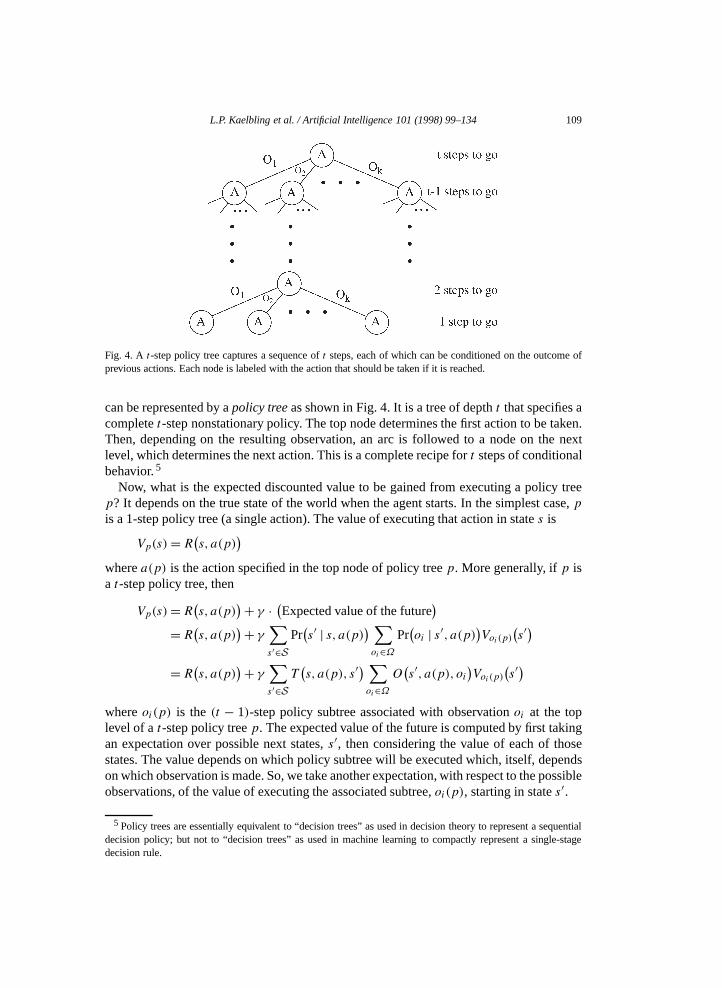
Fig. 4. A t-step policy tree captures a sequence oft steps, each of which can be conditioned on the outcome ofprevious actions. Each node is labeled with the action that should be taken if it is reached.

can be represented by apolicy treeas shown in Fig. 4. It is a tree of deptht that specifies acompletet-step nonstationary policy. The top node determines the first action to be taken.Then, depending on the resulting observation, an arc is followed to a node on the nextlevel, which determines the next action. This is a complete recipe fort steps of conditionalbehavior.5

Now, what is the expected discounted value to be gained from executing a policy treep? It depends on the true state of the world when the agent starts. In the simplest case,p

is a 1-step policy tree (a single action). The value of executing that action in states is

Vp(s)=R(s, a(p)

)wherea(p) is the action specified in the top node of policy treep. More generally, ifp isa t-step policy tree, then

Vp(s)=R(s, a(p)

)+ γ · (Expected value of the future)

=R(s, a(p))+ γ ∑s ′∈S

Pr(s′ | s, a(p)) ∑

oi∈ΩPr(oi | s′, a(p)

)Voi(p)

(s′)

=R(s, a(p))+ γ ∑s ′∈S

T(s, a(p), s′

) ∑oi∈Ω

O(s′, a(p), oi

)Voi(p)

(s′)

whereoi(p) is the (t − 1)-step policy subtree associated with observationoi at the toplevel of at-step policy treep. The expected value of the future is computed by first takingan expectation over possible next states,s′, then considering the value of each of thosestates. The value depends on which policy subtree will be executed which, itself, dependson which observation is made. So, we take another expectation, with respect to the possibleobservations, of the value of executing the associated subtree,oi(p), starting in states′.

5 Policy trees are essentially equivalent to “decision trees” as used in decision theory to represent a sequentialdecision policy; but not to “decision trees” as used in machine learning to compactly represent a single-stagedecision rule.


Because the agent will never know the exact state of the world, it must be able todetermine the value of executing a policy treep from some belief stateb. This is justan expectation over world states of executingp in each state:

Vp(b)=∑s∈S

b(s)Vp(s).

It will be useful, in the following exposition, to express this more compactly. If we letαp = 〈Vp(s1), . . . ,Vp(sn)〉, thenVp(b)= b · αp .

Now we have the value of executing the policy treep in every possible belief state. Toconstruct an optimalt-step nonstationary policy, however, it will generally be necessary toexecute different policy trees from different initial belief states. LetP be the finite set ofall t-step policy trees. Then

Vt(b)=maxp∈P

b · αp.

That is, the optimalt-step value of starting in belief stateb is the value of executing thebest policy tree in that belief state.

This definition of the value function leads us to some important geometric insightsinto its form. Each policy treep induces a value functionVp that is linear inb, andVt is the upper surface of this collection of functions. So,Vt is piecewise-linear andconvex. Fig. 5 illustrates this property. Consider a world with only two states. In sucha world, a belief state consists of a vector of two nonnegative numbers,〈b(s1), b(s2)〉,that sum to 1. Because of this constraint, a single number is sufficient to describe thebelief state. The value function associated with a policy treep1, Vp1, is a linear functionof b(s1) and is shown in the figure as a line. The value functions of other policy treesare similarly represented. Finally,Vt is the maximum of all theVpi at each point inthe belief space, giving us the upper surface, which is drawn in the figure with a boldline.

When there are three world states, a belief state is determined by two values (againbecause of thesimplex constraint, which requires the individual values to be nonnegativeand sum to 1). The belief space can be seen as the triangle in two-space with vertices(0,0),(1,0), and(0,1). The value function associated with a single policy tree is a plane in three

Fig. 5. The optimalt-step value function is the upper surface of the value functions associated with allt-steppolicy trees.


space, and the optimal value function is a bowl shape that is composed of planar facets; atypical example is shown in Fig. 6, but it is possible for the “bowl” to be tipped on its sideor to degenerate to a single plane. This general pattern repeats itself in higher dimensions,but becomes difficult to contemplate and even harder to draw!

The convexity of the optimal value function makes intuitive sense when we thinkabout the value of belief states. States that are in the “middle” of the belief spacehave high entropy—the agent is very uncertain about the real underlying state of theworld. In such belief states, the agent cannot select actions very appropriately and sotends to gain less long-term reward. In low-entropy belief states, which are near thecorners of the simplex, the agent can take actions more likely to be appropriate for thecurrent state of the world and, so, gain more reward. This has some connection to thenotion of “value of information,” [25] where an agent can incur a cost to move it froma high-entropy to a low-entropy state; this is only worthwhile when the value of theinformation (the difference in value between the two states) exceeds the cost of gainingthe information.

Given a piecewise-linear convex value function and thet-step policy trees from whichit was derived, it is straightforward to determine the optimal situation-action mapping forexecution on thet th step from the end. The optimal value function can be projected backdown onto the belief space, yielding a partition into polyhedral regions. Within each region,there is some single policy treep such thatb · αp is maximal over the entire region. Theoptimal action for each belief state in this region isa(p), the action in the root node ofpolicy treep; furthermore, the entire policy treep can be executed from this point byconditioning the choice of further actions directly on observations, without updating the

Fig. 6. A value function in three dimensions is made up of the upper surface of a set of planes.


Fig. 7. The optimalt-step situation-action mapping is determined by projecting the optimal value function backdown onto the belief space.

belief state (though this is not necessarily an efficient way to represent a complex policy).Fig. 7 shows the projection of the optimal value function down into a policy partition inthe two-dimensional example introduced in Fig. 5; over each of the intervals illustrated, asingle policy tree can be executed to maximize expected reward.

4.2. Value functions as sets of vectors

It is possible, in principle, that every possible policy tree might represent the optimalstrategy at some point in the belief space and, hence, that each would contribute to thecomputation of the optimal value function. Luckily, however, this seems rarely to be thecase. There are generally many policy trees whose value functions are totally dominatedby or tied with value functions associated with other policy trees. Fig. 8 shows a situationin which the value function associated with policy treepd is completely dominated by(everywhere less than or equal to) the value function for policy treepb. The situation withthe value function for policy treepc is somewhat more complicated; although it is notcompletely dominated by any single value function, itis completely dominated bypa andpb taken together.

Given a set of policy trees,V, it is possible to define a unique6 minimal subsetV thatrepresents the same value function. We will call this aparsimoniousrepresentation of thevalue function, and say that a policy tree isusefulif it is a component of the parsimoniousrepresentation of the value function.

Given a vector,α, and a set of vectorsV , we defineR(α,V) to be the region of beliefspace over whichα dominates; that is,

R(α,V)= b | b · α > b · α, for all α ∈ V − α andb ∈ B.It is relatively easy, using a linear program, to find a point inR(α,V) if one exists, or todetermine that the region is empty [9].

The simplest pruning strategy, proposed by Sondik [42,58], is to testR(α, V) for everyα in V and remove thoseα that are nowhere dominant. A much more efficient pruning

6 We assume here that two policy trees with the same value function are identical.


Fig. 8. Some policy trees may be totally dominated by others and can be ignored.

method was proposed by Lark and White [64] and is described in detail by Littman [35]and by Cassandra [9]. Because it has many subtle technical details, it is not described here.

4.3. One step of value iteration

The value function for aPOMDP can be computed using value iteration, with the samebasic structure as for the discreteMDP case. The new problem, then, is how to compute aparsimonious representation ofVt from a parsimonious representation ofVt−1.

One of the simplest algorithms for solving this problem [42,58], which we callexhaustive enumeration, works by constructing a large representation ofVt , then pruningit. We let V stand for a set of policy trees, though for each tree we need only actuallystore the top-level action and the vector of values,α. The idea behind this algorithm isthe following:Vt−1, the set of useful(t − 1)-step policy trees, can be used to construct asupersetV+t of the usefult-step policy trees. At-step policy tree is composed of a rootnode with an associated actiona and |Ω| subtrees, each a(t − 1)-step policy tree. Wepropose to restrict our choice of subtrees to those(t −1)-step policy trees that were useful.For any belief state and any choice of policy subtree, there is always a useful subtree that isat least as good at that state; there is never any reason to include a nonuseful policy subtree.

The time complexity of a single iteration of this algorithm can be divided into two parts:generation and pruning. There are|A||Vt−1||Ω| elements inV+t : there are|A| differentways to choose the action and all possible lists of length|Ω| may be chosen from the setVt−1 to form the subtrees. The value functions for the policy trees inV+t can be computedefficiently from those of the subtrees. Pruning requires one linear program for each elementof the starting set of policy trees and does not add to the asymptotic complexity of thealgorithm.

Although it keeps parsimonious representations of the value functions at each step, thisalgorithm still does more much work than may be necessary. Even ifVt is very small, itgoes through the step of generatingV+t , which always has size exponential in|Ω|. In thenext sections, we present the witness algorithm and some complexity analysis, and thenbriefly outline some other algorithms for this problem that attempt to be more efficientthan the approach of exhaustively generatingV+t .


4.4. The witness algorithm

To improve the complexity of the value-iteration algorithm, we must avoid generatingV+t ; instead, we would like to generate the elements ofVt directly. If we could do this, wemight be able to reach a computation time per iteration that is polynomial in|S|, |A|, |Ω|,|Vt−1|, and|Vt |. Cheng [10] and Smallwood and Sondik [56] also try to avoid generating allof V+t by constructingVt directly. However, their algorithms still have worst-case runningtimes exponential in at least one of the problem parameters [34]. In fact, the existence ofan algorithm that runs in time polynomial in|S|, |A|, |Ω|, |Vt−1|, and|Vt | would settlethe long-standing complexity-theoretic question “Does NP = RP?” in the affirmative [34],so we will pursue a slightly different approach.

Instead of computingVt directly, we will compute, for each actiona, a setQat of t-steppolicy trees that have actiona at their root. We can computeVt by taking the union oftheQat sets for all actions and pruning as described in the previous section. Thewitnessalgorithm is a method for computingQat in time polynomial in|S|, |A|, |Ω|, |Vt−1|, and|Qat | (specifically, run time is polynomial in the size of the inputs, the outputs, and animportant intermediate result). It is possible that theQat are exponentially larger thanVt ,but this seems to be rarely the case in practice.

In what sense is the witness algorithm superior to previous algorithms for solvingPOMDPs, then? Experiments indicate that the witness algorithm is faster in practice over awide range of problem sizes [34]. The primary complexity-theoretic difference is that thewitness algorithm runs in polynomial time in the number of policy trees inQat . There areexample problems that cause the other algorithms, although they never construct theQat ’sdirectly, to run in time exponential in the number of policy trees inQat . That means, if werestrict ourselves to problems in which|Qat | is polynomial, that the running time of thewitness algorithm is polynomial. It is worth noting, however, that it is possible to createfamilies of POMDPs that Cheng’s linear support algorithm (sketched in Section 4.5) cansolve in polynomial time that take the witness exponential time to solve; they are problemsin whichS andVt are very small andQat is exponentially larger for some actiona.

From the definition of the state estimator SE and thet-step value functionVt(b), we canexpressQat (b) (recall that this is the value of taking actiona in belief stateb and continuingoptimally for t − 1 steps) formally as

Qat (b)=∑s∈S

b(s)R(s, a)+ γ∑o∈Ω

Pr(o | a,b)Vt−1(b′o)

whereb′o is the belief state resulting from taking actiona and observingo from beliefstate b; that is, b′ = SE(b, a, o). Since V is the value of the best action, we haveVt(b)=maxa Qat (b).

Using arguments similar to those in Section 4.1, we can show that theseQ-functionsare piecewise-linear and convex and can be represented by collections of policy trees. LetQat be the collection of policy trees that specifyQat . Once again, we can define a uniqueminimal useful set of policy trees for eachQ function. Note that the policy trees needed torepresent the functionVt are a subset of the policy trees needed to represent all of theQatfunctions:Vt ⊆⋃aQat . This is because maximizing over actions and then policy trees isthe same as maximizing over the pooled sets of policy trees.


Algorithm 2. Outer loop of the witness algorithm.

V1 := 〈0,0, . . . ,0〉t := 1loop

t := t + 1foreacha in A

Qat :=witness(Vt−1, a)

prune⋃aQat to getVt

until supb |Vt(b)− Vt−1(b)|< εThe code in Algorithm 2 outlines our approach to solvingPOMDPs. The basic structure

remains that of value iteration. At iterationt , the algorithm has a representation of theoptimal t-step value function. Within the value-iteration loop, separateQ-functions foreach action, represented by parsimonious sets of policy trees, are returned by calls towitness using the value function from the previous iteration. The union of these setsforms a representation of the optimal value function. Since there may be extraneous policytrees in the combined set, it is pruned to yield the useful set oft-step policy trees,Vt .

4.4.1. Witness inner loopThe basic structure of the witness algorithm is as follows. We would like to find a

minimal set of policy trees for representingQat for eacha. We consider theQ-functionsone at a time. The setUa of policy trees is initialized with a single policy tree, withactiona at the root, that is the best for some arbitrary belief state (this is easy to do, asdescribed in the following paragraph). At each iteration we ask: Is there some belief stateb for which the true valueQat (b), computed by one-step lookahead usingVt−1, is differentfrom the estimated valueQat (b), computed using the setUa? We call such a belief statea witnessbecause it can, in a sense, testify to the fact that the setUa is not yet a perfectrepresentation ofQat (b). Note that for allb, Qat (b)6Qat (b); the approximation is alwaysan underestimate of the true value function.

Once a witness is identified, we find the policy tree with actiona at the root that willyield the best value at that belief state. To construct this tree, we must find, for eachobservationo, the(t − 1)-step policy tree that should be executed if observationo is madeafter executing actiona. If this happens, the agent will be in belief stateb′ = SE(b, a, o),from which it should execute the(t−1)-step policy treepo ∈ Vt−1 that maximizesVpo(b

′).The treep is built with subtreespo for each observationo. We add the new policy tree toUa to improve the approximation. This process continues until we can prove that no morewitness points exist and therefore that the currentQ-function is perfect.

4.4.2. Identifying a witnessTo find witness points, we must be able to construct and evaluate alternative policy trees.

If p is a t-step policy tree,oi an observation, andp′ a (t − 1)-step policy tree, then wedefinepnew as at-step policy tree that agrees withp in its action and all its subtrees exceptfor observationoi , for which oi(pnew) = p′. Fig. 9 illustrates the relationship betweenpandpnew.


Fig. 9. A new policy tree can be constructed by replacing one of its subtrees.

Now we can state thewitness theorem[34]: The trueQ-function,Qat , differs from theapproximateQ-function,Qat , if and only if there is somep ∈ Ua , o ∈Ω , andp′ ∈ Vt−1

for which there is someb such that

Vpnew(b) > Vp(b), (1)

for all p ∈Ua . That is, if there is a belief state,b, for whichpnew is an improvement overall the policy trees we have found so far, thenb is a witness. Conversely, if none of thetrees can be improved by replacing a single subtree, there are no witness points. A proofof this theorem is included in Appendix A.

4.4.3. Checking the witness conditionThe witness theorem requires us to search for ap ∈ Ua , ano ∈Ω , a p′ ∈ Vt−1 and a

b ∈ B such that condition (1) holds, or to guarantee that no such quadruple exists. SinceUa ,Ω , andVt−1 are finite and (we hope) small, checking all combinations will not be tootime consuming. However, for each combination, we need to search all the belief states totest condition (1). This we can do using linear programming.

For each combination ofp, o andp′ we compute the policy treepnew, as describedabove. For any belief stateb and policy treep ∈Ua , Vpnew(b)−Vp(b) gives the advantageof following policy treepnew instead ofp starting fromb. We would like to find ab thatmaximizes the advantage over all policy treesp the algorithm has found so far.

The linear program in Algorithm 3 solves exactly this problem. The variableδ is theminimum amount of improvement ofpnew over any policy tree inUa at b. It has a set ofconstraints that restrictδ to be a bound on the difference and a set of simplex constraintsthat forceb to be a well-formed belief state. It then seeks to maximize the advantage ofpnew over allp ∈Ua . Since the constraints are all linear, this can be accomplished by linearprogramming. The total size of the linear program is one variable for each component ofthe belief state and one representing the advantage, plus one constraint for each policy treein U , one constraint for each state, and one constraint to ensure that the belief state sumsto one.7

7 In many linear-programming packages, all variables have implicit nonnegativity constraints, so theb(s)> 0constraints are not needed.


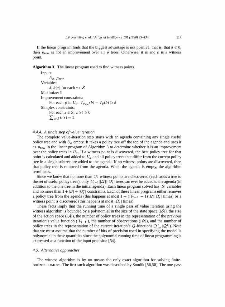
If the linear program finds that the biggest advantage is not positive, that is, thatδ 6 0,thenpnew is not an improvement over allp trees. Otherwise, it is andb is a witnesspoint.

Algorithm 3. The linear program used to find witness points.

Inputs:Ua,pnew

Variables:δ, b(s) for eachs ∈ S

Maximize:δImprovement constraints:

For eachp in Ua: Vpnew(b)− Vp(b)> δSimplex constraints:

For eachs ∈ S: b(s)> 0∑s∈S b(s)= 1

4.4.4. A single step of value iterationThe complete value-iteration step starts with an agenda containing any single useful

policy tree and withUa empty. It takes a policy tree off the top of the agenda and uses itaspnew in the linear program of Algorithm 3 to determine whether it is an improvementover the policy trees inUa . If a witness point is discovered, the best policy tree for thatpoint is calculated and added toUa and all policy trees that differ from the current policytree in a single subtree are added to the agenda. If no witness points are discovered, thenthat policy tree is removed from the agenda. When the agenda is empty, the algorithmterminates.

Since we know that no more thanQat witness points are discovered (each adds a tree tothe set of useful policy trees), only|Vt−1||Ω|||Qat | trees can ever be added to the agenda (inaddition to the one tree in the initial agenda). Each linear program solved has|S| variablesand no more than 1+|S|+ |Qat | constraints. Each of these linear programs either removesa policy tree from the agenda (this happens at most 1+ (|Vt−1| − 1)|Ω||Qat | times) or awitness point is discovered (this happens at most|Qat | times).

These facts imply that the running time of a single pass of value iteration using thewitness algorithm is bounded by a polynomial in the size of the state space (|S|), the sizeof the action space (|A|), the number of policy trees in the representation of the previousiteration’s value function (|Vt−1|), the number of observations (|Ω|), and the number ofpolicy trees in the representation of the current iteration’sQ-functions (

∑a |Qat |). Note

that we must assume that the number of bits of precision used in specifying the model ispolynomial in these quantities since the polynomial running time of linear programming isexpressed as a function of the input precision [54].

4.5. Alternative approaches

The witness algorithm is by no means the only exact algorithm for solving finite-horizonPOMDPs. The first such algorithm was described by Sondik [56,58]. The one-pass


algorithm works by identifying linear regions of the value function one at a time. For eachone, it creates a set of constraints that form the border of the true region, then searchesthose borders to determine whether another region exists beyond the border. Although thealgorithm is sophisticated and, in principle, avoids exhaustively enumerating the set ofpossibly useful policy trees at each iteration, it appears to run more slowly than the simplerenumeration methods in practice, at least for problems with small state spaces [10].

In the process of motivating the one-pass algorithm, Sondik [58] applies the same ideasto findingQ-functions instead of the complete value function. The resulting algorithmmight be called the two-pass algorithm [9], and its form is much like the witness algorithmbecause it first constructs each separateQ-function, then combines theQ-functionstogether to create the optimal value function. Although it appears that the algorithmattracted no attention and was never implemented in over 25 years after the completionof Sondik’s dissertation, it was recently implemented and found to be faster than any of thealgorithms that predated the witness algorithm [9].

As pointed out in Section 4, value functions in belief space have a natural geometricinterpretation. For small state spaces, algorithms that exploit this geometry are quiteefficient [16]. An excellent example of this is Cheng’s linear support algorithm [10]. Thisalgorithm can be viewed as a variation of the witness algorithm in which witness pointsare sought at the corners of regions of the approximate value function defined by thealgorithm’s equivalent of the setU . In two dimensions, these corners can be found easilyand efficiently; the linear support algorithm can be made to run in low-order polynomialtime for problems with two states. In higher dimensions, more complex algorithms areneeded and the number of corners is often exponential in the dimensionality. Thus, thegeometric approaches are useful only inPOMDPs with extremely small state spaces.

Zhang and Liu [67] describe the incremental-pruning algorithm, later generalized byCassandra, Littman, and Zhang [7]. This algorithm is simple to implement and empiricallyfaster than the witness algorithm, while sharing its good worst-case complexity in terms of∑a |Qat |. The basic algorithm works like the exhaustive enumeration algorithm described

in Section 4.3, but differs in that it repeatedly prunes out nonuseful policy trees during thegeneration procedure. As a result, compared to exhaustive enumeration, very few nonusefulpolicy trees are considered and the algorithm runs extremely quickly.

White and Scherer [65] propose an alternative approach in which the reward functionis changed so that all of the algorithms discussed in this chapter will tend to run moreefficiently. This technique has not yet been combined with the witness algorithm, and mayprovide some improvement.

4.6. The infinite horizon

In the previous section, we showed that the optimalt-step value function is alwayspiecewise-linear and convex. This is not necessarily true for the infinite-horizon discountedvalue function; it remains convex [63], but may have infinitely many facets. Still, theoptimal infinite-horizon discounted value function can be approximated arbitrarily closelyby a finite-horizon value function for a sufficiently long horizon [51,59].

The optimal infinite-horizon discounted value function can be approximated via valueiteration, in which the series oft-step discounted value functions is computed; the


iteration is stopped when the difference between two successive results is small, yieldingan arbitrarily good piecewise-linear and convex approximation to the desired valuefunction. From the approximate value function we can extract a stationary policy that isapproximately optimal.

Sondik [59] and Hansen [23] have shown how to use algorithms like the witnessalgorithm that perform exact dynamic-programming backups inPOMDPs in a policy-iteration algorithm to find exact solutions to many infinite-horizon problems.

5. Understanding policies

In this section we introduce a very simple example and use it to illustrate some propertiesof POMDPpolicies. Other examples are explored in an earlier paper [8].

5.1. The tiger problem

Imagine an agent standing in front of two closed doors. Behind one of the doors is a tigerand behind the other is a large reward. If the agent opens the door with the tiger, then alarge penalty is received (presumably in the form of some amount of bodily injury). Insteadof opening one of the two doors, the agent can listen, in order to gain some informationabout the location of the tiger. Unfortunately, listening is not free; in addition, it is alsonot entirely accurate. There is a chance that the agent will hear a tiger behind the left-handdoor when the tiger is really behind the right-hand door, and vice versa.

We refer to the state of the world when the tiger is on the left assl and when it is on theright assr . The actions areLEFT, RIGHT, andLISTEN. The reward for opening the correctdoor is+10 and the penalty for choosing the door with the tiger behind it is−100. Thecost of listening is−1. There are only two possible observations: to hear the tiger on theleft (TL) or to hear the tiger on the right (TR). Immediately after the agent opens a door andreceives a reward or penalty, the problem resets, randomly relocating the tiger behind oneof the two doors.

The transition and observation models can be described in detail as follows. TheLISTEN

action does not change the state of the world. TheLEFT and RIGHT actions cause atransition to world statesl with probability 0.5 and to statesr with probability 0.5(essentially resetting the problem). When the world is in statesl , theLISTEN action resultsin observationTL with probability 0.85 and the observationTR with probability 0.15;conversely for world statesr . No matter what state the world is in, theLEFT andRIGHT

actions result in either observation with probability 0.5.

5.2. Finite-horizon policies

The optimal undiscounted finite-horizon policies for the tiger problem are rather strikingin the richness of their structure. Let us begin with the situation-action mapping for thetime stept = 1, when the agent only gets to make a single decision. If the agent believeswith high probability that the tiger is on the left, then the best action is to open the rightdoor; if it believes that the tiger is on the right, the best action is to open the left door.


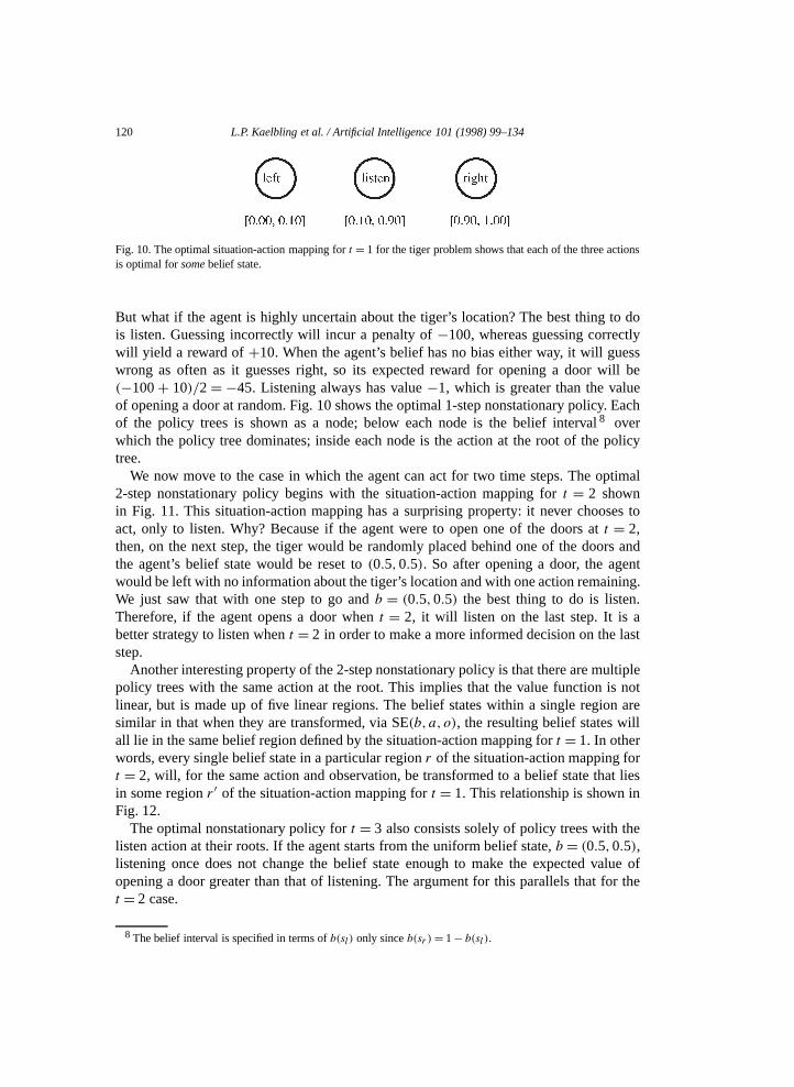
Fig. 10. The optimal situation-action mapping fort = 1 for the tiger problem shows that each of the three actionsis optimal forsomebelief state.

But what if the agent is highly uncertain about the tiger’s location? The best thing to dois listen. Guessing incorrectly will incur a penalty of−100, whereas guessing correctlywill yield a reward of+10. When the agent’s belief has no bias either way, it will guesswrong as often as it guesses right, so its expected reward for opening a door will be(−100+ 10)/2= −45. Listening always has value−1, which is greater than the valueof opening a door at random. Fig. 10 shows the optimal 1-step nonstationary policy. Eachof the policy trees is shown as a node; below each node is the belief interval8 overwhich the policy tree dominates; inside each node is the action at the root of the policytree.

We now move to the case in which the agent can act for two time steps. The optimal2-step nonstationary policy begins with the situation-action mapping fort = 2 shownin Fig. 11. This situation-action mapping has a surprising property: it never chooses toact, only to listen. Why? Because if the agent were to open one of the doors att = 2,then, on the next step, the tiger would be randomly placed behind one of the doors andthe agent’s belief state would be reset to(0.5,0.5). So after opening a door, the agentwould be left with no information about the tiger’s location and with one action remaining.We just saw that with one step to go andb = (0.5,0.5) the best thing to do is listen.Therefore, if the agent opens a door whent = 2, it will listen on the last step. It is abetter strategy to listen whent = 2 in order to make a more informed decision on the laststep.

Another interesting property of the 2-step nonstationary policy is that there are multiplepolicy trees with the same action at the root. This implies that the value function is notlinear, but is made up of five linear regions. The belief states within a single region aresimilar in that when they are transformed, via SE(b, a, o), the resulting belief states willall lie in the same belief region defined by the situation-action mapping fort = 1. In otherwords, every single belief state in a particular regionr of the situation-action mapping fort = 2, will, for the same action and observation, be transformed to a belief state that liesin some regionr ′ of the situation-action mapping fort = 1. This relationship is shown inFig. 12.

The optimal nonstationary policy fort = 3 also consists solely of policy trees with thelisten action at their roots. If the agent starts from the uniform belief state,b = (0.5,0.5),listening once does not change the belief state enough to make the expected value ofopening a door greater than that of listening. The argument for this parallels that for thet = 2 case.

8 The belief interval is specified in terms ofb(sl) only sinceb(sr )= 1− b(sl ).


Fig. 11. The optimal situation-action mapping fort = 2 in the tiger problem consists only of theLISTEN action.

Fig. 12. The optimal nonstationary policy fort = 2 illustrates belief state transformations fromt = 2 to t = 1. Itconsists of five separate policy trees.

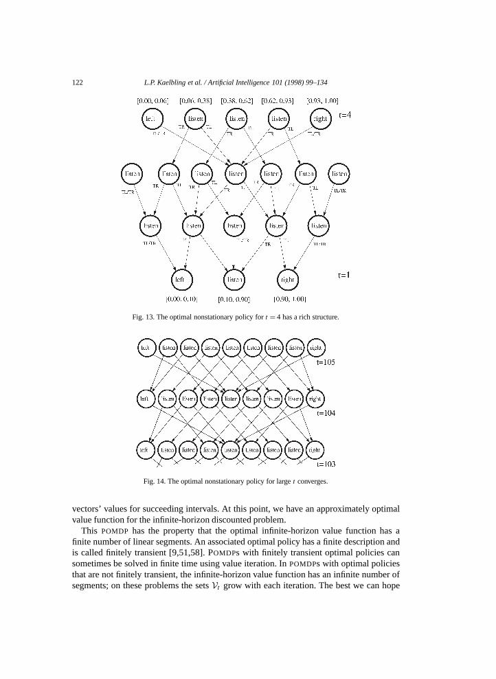
This argument for listening in the first steps no longer applies aftert = 3; the optimalsituation-action mappings fort > 3 all choose to open a door for some belief states. Fig. 13shows the structure that emerges in the optimal nonstationary policy fort = 4. Notice thatfor t = 3 there are two nodes that do not have any incoming arcs fromt = 4. This happensbecause there is no belief state att = 4 for which the optimal action and any resultingobservation generates a new belief state that lies in either of the regions defined by theunused nodes att = 3.

This graph can also be interpreted as a compact representation of all of the useful policytrees at every level. The forest of policy trees is transformed into a directed acyclic graphby collapsing all of the nodes that stand for the same policy tree into one.

5.3. Infinite-horizon policies

When we include a discount factor to decrease the value of future rewards, the structureof the finite-horizonPOMDP value function changes slightly. As the horizont increases,the rewards received for the final few steps have decreasing influence on the situation-action mappings for earlier time steps and the value function begins to converge. In manydiscountedPOMDPproblems, the optimal situation-action mapping for larget looks muchthe same as the optimal situation-action mapping fort − 1. Fig. 14 shows a portion of theoptimal nonstationary policy for thediscountedfinite-horizon version of the tiger problemfor large values oft . Notice that the structure of the graph is exactly the same from one timeto the next. The vectors for each of the nodes, which together define the value function,differ only after the fifteenth decimal place. This structure first appears at time stept = 56and remains constant throught = 105. Whent = 105, the precision of the algorithm usedto calculate the situation-action mappings can no longer discern any difference between the


Fig. 13. The optimal nonstationary policy fort = 4 has a rich structure.

Fig. 14. The optimal nonstationary policy for larget converges.

vectors’ values for succeeding intervals. At this point, we have an approximately optimalvalue function for the infinite-horizon discounted problem.

This POMDP has the property that the optimal infinite-horizon value function has afinite number of linear segments. An associated optimal policy has a finite description andis called finitely transient [9,51,58]. POMDPs with finitely transient optimal policies cansometimes be solved in finite time using value iteration. InPOMDPs with optimal policiesthat are not finitely transient, the infinite-horizon value function has an infinite number ofsegments; on these problems the setsVt grow with each iteration. The best we can hope


for is to solve thesePOMDPs approximately. It is not known whether there is a way ofusing the value-iteration approach described in this paper for solvingall POMDPs withfinitely transient optimal policies in finite time; we conjecture that there is. The only finite-time algorithm that has been described for solvingPOMDPs with finitely transient optimalpolicies over the infinite horizon is a version of policy iteration described by Sondik [58].The simpler policy-iteration algorithm due to Hansen [23] has not been proven to convergefor all suchPOMDPs.9

5.4. Plan graphs

One drawback of thePOMDP approach is that the agent must maintain a belief stateand use it to select an optimal action on every step; if the underlying state space orVis large, then this computation can be expensive. In many cases, it is possible to encodethe policy in a graph that can be used to select actions without any explicit representationof the belief state [59]; we refer to such graphs asplan graphs. Recall Fig. 14, in whichthe algorithm has nearly converged upon an infinite-horizon policy for the tiger problem.Because the situation-action mappings at every level have the same structure, we can makethe nonstationary policy into a stationary one by redrawing the edges from one level toitself as if it were the succeeding level. This rearrangement of edges is shown in Fig. 15,and the result is redrawn in Fig. 16 as a plan graph.

Some of the nodes of the graph will never be visited once either door is opened and thebelief state is reset to(0.5,0.5). If the agent always starts in a state of complete uncertainty,then it will never be in a belief state that lies in the region of these nonreachable nodes.This results in a simpler version of the plan graph, shown in Fig. 17. The plan graph has asimple interpretation: keep listening until you have heard the tiger twice more on one sidethan the other.

Because the nodes represent a partition of the belief space and because all belief stateswithin a particular region will map to a single node on the next level, the plan graphrepresentation does not require the agent to maintain an on-line representation of the beliefstate; the current node is a sufficient representation of the current belief. In order to executea plan graph, the initial belief state is used to choose a starting node. After that, the agentneed only maintain a pointer to a current node in the graph. On every step, it takes the actionspecified by the current node, receives an observation, then follows the arc associated withthat observation to a new node. This process continues indefinitely.

A plan graph is essentially a finite-state controller. It uses the minimal possible amountof memory to act optimally in a partially observable environment. It is a surprisingand pleasing result that it is possible to start with a discrete problem, reformulate it interms of a continuous belief space, then map the continuous solution back into a discrete

9 As a technical aside, if there arePOMDPs that have finitely transient optimal policies for which neither valueiteration nor Hansen’s policy-iteration algorithm converges, the tiger problem is a good candidate. This is becausethe behavior of these algorithms on this problem appears to be extremely sensitive to the numerical precision usedin comparisons—the better the precision, the longer the algorithms take to converge. In fact, it may be the case thatimprecision isnecessaryfor the algorithms to converge on this problem, although it is difficult to test this withoutdetailed formal analysis. Sondik’s proof that his policy-iteration algorithm converges depends on controlled useof imprecision and we have not studied how that could best be used in the context of value iteration.


Fig. 15. Edges can be rearranged to form a stationary policy.

Fig. 16. The optimal infinite-horizon policy for the tiger problem can be drawn as a plan graph. This structurecounts the relative number of times the tiger was heard on the left as compared to the right.

Fig. 17. Given the initial belief state of(0.5,0.5) for the tiger problem, some nodes of the plan graph can betrimmed.


Fig. 18. More memory is needed in the tiger problem when listening reliability is reduced to 0.65.

controller. Furthermore, the extraction of the controller can be done automatically fromtwo successive equal value functions.

It is also important to note that there is no knowna priori bound on the size of theoptimal plan graph in terms of the size of the problem. In the tiger problem, for instance, ifthe probability of getting correct information from theLISTEN action is reduced from 0.85to 0.65, then the optimal plan graph, shown in Fig. 18, is much larger, because the agentmust hear the tiger on one side 5 times more than in the other before being sufficientlyconfident to act. As the observation reliability decreases, an increasing amount of memoryis required.

6. Related work

In this section, we examine how the assumptions of thePOMDP model relate to earlierwork on planning in AI. We consider only models with finite-state and action spaces andstatic underlying dynamics, as these assumptions are consistent with the majority of workin this area. Our comparison focuses on issues of imperfect knowledge, uncertainty ininitial state, the transition model, the observation model, the objective of planning, therepresentation of domains, and plan structures. The most closely related work to our ownis that of Kushmerick, Hanks, and Weld [30] on the BURIDAN system, and Draper, Hanksand Weld [14] on the C-BURIDAN system.

6.1. Imperfect knowledge

Plans generated using standardMDP algorithms and classical planning algorithms10

assume that the underlying state of the process will be known with certainty during planexecution. In theMDP framework, the agent is informed of the current state each time ittakes an action. In many classical planners (e.g.,SNLP [39], UCPOP[45]), the current state

10 By “classical planning” we mean linear or partial-order planners using STRIPS-like operators.


can be calculated trivially from the known initial state and knowledge of the deterministicoperators.

The assumption of perfect knowledge is not valid in many domains. Research onepistemic logic [43,44,52] relaxes this assumption by making it possible to reason aboutwhat is and is not known at a given time. Unfortunately, epistemic logics have not beenused as a representation in automatic planning systems, perhaps because the richness ofrepresentation they provide makes efficient reasoning very difficult.

A step towards building a working planning system that reasons about knowledge is torelax the generality of the logic-based schemes. The approach ofCNLP [46] uses three-valued propositions where, in addition to true and false, there is a valueunknown, whichrepresents the state when the truth of the proposition is not known. Operators can thenrefer to whether propositions have anunknownvalue in their preconditions and can havethe value in their effects. This representation for imperfect knowledge is only appropriatewhen the designer of the system knows, in advance, what aspects of the state will be knownand unknown. It is insufficient for multiple agents reasoning about each others’ knowledgeand for representing certain types of correlated uncertainty [20].

Formulating knowledge as predicate values that are either known or unknown makesit impossible to reason about gradations of knowledge. For example, an agent that isfairly certain that it knows the combination to a lock might be willing to try to unlock itbefore seeking out more precise knowledge. Reasoning about levels of knowledge is quitecommon and natural in thePOMDP framework. As long as an agent’s state of knowledgecan be expressed as a probability distribution over possible states of the world, thePOMDP

perspective applies.

6.2. Initial state

Many classical planning systems (SNLP, UCPOP, CNLP) require the starting state to beknown during the planning phase. An exception is the U-PLAN [38] system, which createsa separate plan for each possible initial state with the aim of making these plans easy tomerge to form a single plan. Conditional planners typically have some aspects of the initialstate unknown. If these aspects are important to the planning process, they are tested duringexecution.

In the POMDP framework, the starting state is not required to be known precisely andcan instead be represented as a probability distribution over possible states. BURIDAN andC-BURIDAN also use probability distributions over states as an internal representation ofuncertainty, so they can deal with initial-state uncertainty in much the same way.

6.3. Transition model

In classical planning systems, operators have deterministic effects. The plans constructedare brittle, since they apply to a specific starting state and require the trajectory through thestates to go exactly as expected. Many domains are not easily modeled with deterministicactions, since an action can have different results, even when applied in exactly the samestate.


Extensions to classical planning, such asCNLP [46] and CASSANDRA [48] have consid-ered operators with nondeterministic effects. For each operator, there is a set of possiblenext states that could occur. A drawback of this approach is that it gives no informationabout the relative likelihood of the possible outcomes. These systems plan for every possi-ble contingency to ensure that the resulting plan is guaranteed to lead to a goal state.

Another approach used in modeling nondeterministic actions is to define a probabilitydistribution over the possible next states. This makes it possible to reason about which ofthe resulting states are more likely and makes it possible to assess whether a plan islikely toreach the goal even if it is not guaranteed to do so. This type of action model is used inMDPsand POMDPs as well as in BURIDAN and C-BURIDAN. Other work [5,15,19] has usedrepresentations that can be used to compute probability distributions over future states.

6.4. Observation model

When the starting state is known and actions are deterministic, there is no need to getfeedback from the environment when executing a plan. However, if the starting state isunknown or the actions have nondeterministic effects, more effective plans can be built byexploiting feedback, or observations, from the environment concerning the identity of thecurrent state.

If observations reveal the precise identity of the current state, the planning model iscalled “completely observable.” TheMDP model, as well as some planning systems suchas CNLP and PLINTH [18,19] assume complete observability. Other systems, such asBURIDAN and MAXPLAN [37], have no observation model and can attack “completelyunobservable” problems. Classical planning systems typically have no observation model,but the fact that the initial state is known and operators are deterministic means that theycan also be thought of as solving completely observable problems.

Completely observable and completely unobservable models are particularly clean butare unrealistic. ThePOMDP and C-BURIDAN frameworks modelpartially observableenvironments, in that observations provide some information about the underlying state,but not enough to guarantee that it will be known with certainty. This model provides fora great deal of expressiveness (both completely observable and completely unobservablemodels can be viewed as special cases), but is quite difficult to solve. It is an interestingand powerful model because it allows systems to reason about taking actions to gatherknowledge that will be important for later decision making.

6.5. Objective

The job of a planner is to find a plan that satisfies a particular objective; most often, theobjective is a goal of achievement, that is, to arrive at some state that is in a set of problem-specific goal states. When probabilistic information is available concerning the initial stateand transitions, a more general objective can be used—reaching a goal state with sufficientprobability (see, for example, work on BURIDAN and C-BURIDAN).

A popular alternative to goal attainment is maximizing total expected discounted reward(total-reward criterion). Under this objective, each action results in an immediate rewardthat is a function of the current state. The exponentially discounted sum of these rewards


over the execution of a plan (finite or infinite horizon) constitutes the value of the plan.This objective is used extensively in most work withMDPs andPOMDPs, including ours.

Several authors (for example, Koenig [27]) have pointed out that, given a completelyobservable problem stated as one of goal achievement, reward functions can be constructedso that a policy that maximizes reward can be used to maximize the probability of goalattainment in the original problem. This shows that the total-reward criterion is no lessgeneral than goal achievement in completely observable domains. The same holds forfinite-horizon partially observable domains.

Interestingly, a more complicated transformation holds in the opposite direction: anytotal expected discounted reward problem (completely observable or finite horizon) canbe transformed into a goal-achievement problem of similar size [12,69]. Roughly, thetransformation simulates the discount factor by introducing an absorbing state with a smallprobability of being entered on each step. Rewards are then simulated by normalizing allreward values to be between zero and one and then “siphoning off” some of the probabilityof absorption equal to the amount of normalized reward. The (perhaps counterintuitive)conclusion is that goal-attainment problems and reward-type problems are computationallyequivalent.

There is a qualitative difference in the kinds of problems typically addressed withPOMDPmodels and those addressed with planning models. Quite frequently,POMDPs areused to model situations in which the agent is expected to go on behaving indefinitely,rather than simply until a goal is achieved. Given the inter-representability results betweengoal-probability problems and discounted-optimality problems, it is hard to make technicalsense of this difference. In fact, manyPOMDPmodels should probably be addressed in anaverage-reward context [17]. Using a discounted-optimal policy in a truly infinite-durationsetting is a convenient approximation, similar to the use of a situation-action mapping froma finite-horizon policy in receding horizon control.

Littman [35] catalogs some alternatives to the total-reward criterion, all of which arebased on the idea that the objective value for a plan is based on a summary of immediaterewards over the duration of a run. Koenig and Simmons [28] examine risk-sensitiveplanning and showed how planners for the total-reward criterion could be used to optimizerisk-sensitive behavior. Haddawy et al. [21] looked at a broad family of decision-theoreticobjectives that make it possible to specify trade-offs between partially satisfying goalsquickly and satisfying them completely. Bacchus, Boutilier and Grove [2] show how somericher objectives based on evaluations of sequences of actions can actually be converted tototal-reward problems. Other objectives considered in planning systems, aside from simplegoals of achievement, include goals of maintenance and goals of prevention [15]; thesetypes of goals can typically be represented using immediate rewards as well.

6.6. Representation of problems

The propositional representations most often used in planning have a number ofadvantages over the flat state-space representations associated withMDPs andPOMDPs. Themain advantage comes from their compactness—just as with operator schemata, which canrepresent many individual actions in a single operator, propositional representations can beexponentially more concise than a fully expanded state-based transition matrix for anMDP.


Algorithms for manipulating compact (or factored)POMDPs have begun to ap-pear [6,14]—this is a promising area for future research. At present, however, there isno evidence that these algorithms result in improved planning time significantly over theuse of a “flat” representation of the state space.

6.7. Plan structures

Planning systems differ in the structure of the plans they produce. It is important thata planner be able to express the optimal plan if one exists for a given domain. We brieflyreview some popular plan structures along with domains in which they are sufficient forexpressing optimal behavior.

Traditional plans are simple sequences of actions. They are sufficient when the initialstate is known and all actions are deterministic. A slightly more elaborate structure isthe partially ordered plan (generated, for example, bySNLP and UCPOP), or the parallelplan [4]. In this type of plan, actions can be left unordered if all orderings are equivalentunder the performance metric.

When actions are stochastic, partially ordered plans can still be used (as in BURIDAN),but contingent plans can be more effective. The simplest kind of contingent or branchingplan is one that has a tree structure (as generated byCNLP or PLINTH). In such a plan,some of the actions have different possible outcomes that can be observed, and the flowof execution of the plan is conditioned on the outcome. Branching plans are sufficientfor representing optimal plans for finite-horizon domains. Directed acyclic graphs (DAGs)can represent the same class of plans, but potentially do so much more succinctly, becauseseparate branches can share structure. C-BURIDAN uses a representation of contingentplans that also allows for structure sharing (although of a different type than our DAG-structured plans). Our work onPOMDPs finds DAG-structured plans for finite-horizonproblems.

For infinite-horizon problems, it is necessary to introduce loops into the plan represen-tation [31,57]. (Loops might also be useful in long finite-horizonPOMDPs for representa-tional succinctness.) A simple loop-based plan representation depicts a plan as a labeleddirected graph. Each node of the graph is labeled with an action and there is one labeledoutgoing edge for each possible outcome of the action. It is possible to generate this typeof plan graphfor somePOMDPs [8,22,23,47,59].

For completely observable problems with a high branching factor, a more convenientrepresentation is apolicy, which maps the current state (situation) to a choice of action.Because there is an action choice specified for all possible initial states, policies arealso called universal plans [53]. This representation is not appropriate forPOMDPs, sincethe underlying state is not fully observable. However,POMDP policies can be viewed asuniversal plans over belief space.

It is interesting to note that there are infinite-horizonPOMDPs for which no finite-stateplan is sufficient. Simple 2-state examples can be constructed for which optimal behaviorrequires counting (i.e., a simple stack machine); there is reason to believe that generalpushdown automata and perhaps even Turing machines are necessary to represent optimalplans in general. This argues that, in the limit, a plan is actually a program. Severaltechniques have been proposed recently for searching for good program-like controllers


in POMDPs [29,68]. We restrict our attention to the simpler finite-horizon case and a smallset of infinite-horizon problems that have optimal finite-state plans.

7. Extensions and conclusions

ThePOMDPmodel provides a firm foundation for work on planning under uncertainty inaction and observation. It gives a uniform treatment of action to gain information and actionto change the world. Although they are derived through the domain of continuous beliefspaces, elegant finite-state controllers may sometimes be constructed using algorithms suchas the witness algorithm.

However, experimental results [34] suggest that even the witness algorithm becomesimpractical for problems of modest size (|S| > 15 and |Ω| > 15). Our current workexplores the use of function-approximation methods for representing value functions andthe use of simulation in order to concentrate the approximations on the frequently visitedparts of the belief space [33]. The results of this work are encouraging and have allowed usto get a very good solution to an 89-state, 16-observation instance of a hallway navigationproblem similar to the one described in the introduction. We are optimistic and hope toextend these techniques (and others) to get good solutions to large problems.

Another area that is not addressed in this paper is the acquisition of a world model.One approach is to extend techniques for learning hidden Markov models [50,60] to learnPOMDP models. Then, we could apply algorithms of the type described in this paperto the learned models. Another approach is to combine the learning of the model withthe computation of the policy. This approach has the potential significant advantage ofbeing able to learn a model that is complex enough to support optimal (or good) behaviorwithout making irrelevant distinctions; this idea has been pursued by Chrisman [11] andMcCallum [40,41].

Appendix A

Theorem A.1. LetUa be a nonempty set of useful policy trees, andQat be the complete setof useful policy trees. ThenUa 6=Qat if and only if there is some treep ∈ Ua , observationo∗ ∈Ω , and subtreep′ ∈ Vt−1 for which there is some belief stateb such that

Vpnew(b) > Vp(b) (A.1)

for all p ∈Ua , wherepnew is a t-step policy tree that agrees withp in its action and all itssubtrees except for observationo∗, for whicho∗(pnew)= p′.

Note that we are defining two trees to be equal if they have the same value function; thismakes it unnecessary to deal with the effect of ties in the setUa .

Proof. The “if” direction is easy since theb can be used to identify a policy tree missingfromUa .

The “only if” direction can be rephrased as: IfUa 6=Qat then there is a belief stateb, ap ∈Ua , and apnew such thatpnew has a larger value than any otherp ∈Ua at b.


Start by picking somep∗ ∈Qat −Ua and choose anyb such thatp∗ has the highest valueatb (there must be such ab sincep∗ is useful). Let

p = argmaxp′∈Ua

Vp′(b).

Now, p∗ is the policy tree inQat −Ua that has the highest value atb, andp is the policytree inUa that has the highest value atb. By construction,Vp∗(b) > Vp(b).

Now, if p andp∗ differ in only one subtree, then we are done,p∗ can serve as apnew inthe theorem.

If p andp∗ differ in more than one subtree, we will identify another policy tree that canact aspnew. Choose an observationo∗ ∈Ω such that∑

s

b(s)

(∑s ′∈S

T(s, a

(p∗), s′)Vo∗(p∗)

(s′))

>∑s

b(s)

(∑s ′∈S

T(s, a

(p∗), s′)Vo∗(p)

(s′)).

There must be ao∗ satisfying this inequality since otherwise we get the contradiction

Vp∗(b)

=∑s

b(s)

(R(s, a

(p∗))+ γ ∑

s ′∈ST(s, a

(p∗), s′) ∑oi∈Ω

O(s′, a

(p∗), oi)Voi(p∗)

(s′))

6∑s

b(s)

(R(s, a(p)

)+ γ ∑s ′∈S

T(s, a(p), s′

) ∑oi∈Ω

O(s′, a(p), oi

)Voi(p)

(s′))

= Vp(b).Definepnew to be identical top except that in the place of subtreeo∗(p), we puto∗(p∗).From this, it follows that

Vpnew(b)=∑s

b(s)

(R(s, a(pnew)

)+ γ

∑s ′∈S

T(s, a(pnew), s

′) ∑oi∈Ω

O(s′, a(pnew), oi

)Voi(pnew)

(s′))

>∑s

b(s)

(R(s, a(p)

)+ γ

∑s ′∈S

T(s, a(p), s′

) ∑oi∈Ω

O(s′, a(p), oi

)Voi(p)

(s′))

= Vp(b)> Vp(b)for all p ∈Ua . Therefore, the policy treesp andpnew, the observationo∗, p′ = o∗(p∗) andthe belief stateb satisfy the conditions of the theorem.2


References

[1] K.J. Aström, Optimal control of Markov decision processes with incomplete state estimation, J. Math. Anal.Appl. 10 (1995) 174–205.

[2] F. Bacchus, C. Boutilier and A. Grove, Rewarding behaviors, in: Proceedings Thirteenth NationalConference on Artificial Intelligence (AAAI-96), Portland, OR, AAAI Press/MIT Press, Menlo Park, CA,1996, pp. 1160–1167.

[3] D.P. Bertsekas, Dynamic Programming and Optimal Control, Vols. 1 and 2, Athena Scientific, Belmont,MA, 1995.

[4] A.L. Blum and M.L. Furst, Fast planning through planning graph analysis, Artificial Intelligence 90 (1–2)(1997) 279–298.

[5] J. Blythe, Planning with external events, in: Proceedings Tenth Conference on Uncertainty in ArtificialIntelligence (UAI-94), Seattle, WA, 1994, pp. 94–101.

[6] C. Boutilier and D. Poole, Computing optimal policies for partially observable decision processes usingcompact representations, in: Proceedings Thirteenth National Conference on Artificial Intelligence (AAAI-96), Portland, OR, AAAI Press/MIT Press, Menlo Park, CA, 1996, pp. 1168–1175.

[7] A. Cassandra, M.L. Littman and N.L. Zhang, Incremental Pruning: a simple, fast, exact method for partiallyobservable Markov decision processes, in: Proceedings Thirteenth Annual Conference on Uncertainty inArtificial Intelligence (UAI–97), Morgan Kaufmann, San Francisco, CA, 1997, pp. 54–61.

[8] A.R. Cassandra, L.P. Kaelbling and M.L. Littman, Acting optimally in partially observable stochasticdomains, in: Proceedings Twelfth National Conference on Artificial Intelligence (AAAI-94), Seattle, WA,1994, pp. 1023–1028.

[9] A.R. Cassandra, Exact and approximate algorithms for partially observable Markov decision problems,Ph.D. Thesis, Department of Computer Science, Brown University, Providence, RI, 1998.

[10] H.-T. Cheng, Algorithms for partially observable Markov decision processes, Ph.D. Thesis, University ofBritish Columbia, Vancouver, BC, 1988.

[11] L. Chrisman, Reinforcement learning with perceptual aliasing: The perceptual distinctions approach, in:Proceedings Tenth National Conference on Artificial Intelligence (AAAI-92), San Jose, CA, AAAI Press,San Jose, CA, 1992, pp. 183–188.

[12] A. Condon, The complexity of stochastic games, Inform. and Comput. 96 (2) (1992) 203–224.[13] T. Dean, L.P. Kaelbling, J. Kirman and A. Nicholson, Planning under time constraints in stochastic domains,

Artificial Intelligence 76 (1–2) (1995) 35–74.[14] D. Draper, S. Hanks and D. Weld, Probabilistic planning with information gathering and contingent

execution, Technical Report 93-12-04, University of Washington, Seattle, WA, 1993.[15] M. Drummond and J. Bresina, Anytime synthetic projection: maximizing the probability of goal satisfaction,

in: Proceedings Eighth National Conference on Artificial Intelligence (AAAI-90), Boston, MA, MorganKaufmann, San Francisco, CA, 1990, pp. 138–144.

[16] J.N. Eagle, The optimal search for a moving target when the search path is constrained, Oper. Res. 32 (5)(1984) 1107–1115.

[17] E. Fernández-Gaucherand, A. Arapostathis and S.I. Marcus, On the average cost optimality equation and thestructure of optimal policies for partially observable Markov processes, Ann. Oper. Res. 29 (1991) 471–512.

[18] R.P. Goldman and M.S. Boddy, Conditional linear planning, in: K. Hammond (Ed.), The SecondInternational Conference on Artificial Intelligence Planning Systems, AAAI Press/MIT Press, Menlo Park,CA, 1994, pp. 80–85.

[19] R.P. Goldman and M.S. Boddy, Epsilon-safe planning, in: Proceedings 10th Conference on Uncertainty inArtificial Intelligence (UAI-94), Seattle, WA, 1994, pp. 253–261.

[20] R.P. Goldman and M.S. Boddy, Representing uncertainty in simple planners, in: Proceedings 4thInternational Conference on Principles of Knowledge Representation and Reasoning (KR-94), Bonn,Germany, 1994, pp. 238–245.

[21] P. Haddawy and S. Hanks, Utility models for goal-directed decision-theoretic planners, Technical Report93-06-04, Department of Computer Science and Engineering, University of Washington, 1993.

[22] E.A. Hansen, Cost-effective sensing during plan execution, in: Proceedings Twelfth National Conference onArtificial Intelligence (AAAI-94), Seattle, WA, AAAI Press/MIT Press, Menlo Park, CA, 1994, pp. 1029–1035.


[23] E.A. Hansen, An improved policy iteration algorithm for partially observable MDPs, in: Advances in NeuralInformation Processing Systems 10 (1998).

[24] R.A. Howard, Dynamic Programming and Markov Processes, MIT Press, Cambridge, MA, 1960.[25] R.A. Howard, Information value theory, IEEE Trans. Systems Science and Cybernetics SSC-2 (1) (1966)

22–26.[26] R.E. Kalman, A new approach to linear filtering and prediction problems, Trans. American Society of

Mechanical Engineers, Journal of Basic Engineering 82 (1960) 35–45.[27] S. Koenig, Optimal probabilistic and decision-theoretic planning using Markovian decision theory, Technical

Report UCB/CSD 92/685, Berkeley, CA, 1992.[28] S. Koenig and R.G. Simmons, Risk-sensitive planning with probabilistic decision graphs, in: Proceedings

4th International Conference on Principles of Knowledge Representation and Reasoning (KR-94), Bonn,Germany, 1994, pp. 363–373.

[29] J.R. Koza, Genetic Programming: On the Programming of Computers by Means of Natural Selection, MITPress, Cambridge, MA, 1992.

[30] N. Kushmerick, S. Hanks and D.S. Weld, An algorithm for probabilistic planning, Artificial Intelligence 76(1–2) (1995) 239–286.

[31] S.-H. Lin and T. Dean, Generating optimal policies for high-level plans with conditional branches and loops,in: Proceedings Third European Workshop on Planning (1995) 205–218.

[32] M.L. Littman, Memoryless policies: theoretical limitations and practical results, in: D. Cliff, P. Husbands,J.-A. Meyer and S.W. Wilson (Eds.), From Animals to Animats 3: Proceedings Third InternationalConference on Simulation of Adaptive Behavior, MIT Press, Cambridge, MA, 1994.

[33] M.L. Littman, A.R. Cassandra and L.P. Kaelbling, Learning policies for partially observable environments:scaling up, in: A. Prieditis and S. Russell (Eds.), Proceedings Twelfth International Conference on MachineLearning, Morgan Kaufmann, San Francisco, CA, 1995, pp. 362–370. Reprinted in: M.H. Huhns andM.P. Singh (Eds.), Readings in Agents, Morgan Kaufmann, San Francisco, CA, 1998.

[34] M.L. Littman, A.R. Cassandra and L.P. Kaelbling, Efficient dynamic-programming updates in partiallyobservable Markov decision processes, Technical Report CS-95-19, Brown University, Providence, RI,1996.

[35] M.L. Littman, Algorithms for sequential decision making, Ph.D. Thesis, Department of Computer Science,Brown University, 1996; also Technical Report CS-96-09.

[36] W.S. Lovejoy, A survey of algorithmic methods for partially observable Markov decision processes, Ann.Oper. Res. 28 (1) (1991) 47–65.

[37] S.M. Majercik and M.L. Littman, MAXPLAN: a new approach to probabilistic planning, Technical ReportCS-1998-01, Department of Computer Science, Duke University, Durham, NC, 1998; submitted for review.

[38] T.M. Mansell, A method for planning given uncertain and incomplete information, in: Proceedings 9thConference on Uncertainty in Artificial Intelligence (UAI-93), Morgan Kaufmann, San Mateo, CA, 1993,pp. 350–358.

[39] D. McAllester and D. Rosenblitt, Systematic nonlinear planning, in: Proceedings 9th National Conferenceon Artificial Intelligence (AAAI-91), Anaheim, CA, 1991, pp. 634–639.

[40] R.A. McCallum, Overcoming incomplete perception with utile distinction memory, in: Proceedings TenthInternational Conference on Machine Learning, Morgan Kaufmann, Amherst, MA, 1993, pp. 190–196.

[41] R.A. McCallum, Instance-based utile distinctions for reinforcement learning with hidden state, in:Proceedings Twelfth International Conference on Machine Learning, Morgan Kaufmann, San Francisco,CA, 1995, pp. 387–395.

[42] G.E. Monahan, A survey of partially observable Markov decision processes: theory, models, and algorithms,Management Science 28 (1) (1982) 1–16.

[43] R.C. Moore, A formal theory of knowledge and action, in: J.R. Hobbs and R.C. Moore (Eds.), FormalTheories of the Commonsense World, Ablex Publishing, Norwood, NJ, 1985, pp. 319–358.

[44] L. Morgenstern, Knowledge preconditions for actions and plans, in: Proceedings 10th International JointConference on Artificial Intelligence (IJCAI-87), Milan, Italy, 1987, pp. 867–874.

[45] J.S. Penberthy and D. Weld, UCPOP: a sound, complete, partial order planner for ADL, in: ProceedingsThird International Conference on Principles of Knowledge Representation and Reasoning (KR-92),Cambridge, MA, 1992, pp. 103–114.


[46] M.A. Peot and D.E. Smith, Conditional nonlinear planning, in: Proceedings First International Conferenceon Artificial Intelligence Planning Systems, 1992, pp. 189–197.

[47] L.K. Platzman, A feasible computational approach to infinite-horizon partially-observed Markov decisionproblems, Technical Report, Georgia Institute of Technology, Atlanta, GA, 1981.

[48] L. Pryor and G. Collins, Planning for contingencies: a decision-based approach, J. Artif. Intell. Res. 4 (1996)287–339.

[49] M.L. Puterman, Markov Decision Processes—Discrete Stochastic Dynamic Programming, Wiley, NewYork, NY, 1994.

[50] L.R. Rabiner, A tutorial on hidden Markov models and selected applications in speech recognition, Proc.IEEE 77 (2) (1989) 257–286.

[51] K. Sawaki and A. Ichikawa, Optimal control for partially observable Markov decision processes over aninfinite horizon, J. Oper. Res. Soc. Japan 21 (1) (1978) 1–14.

[52] R.B. Scherl and H.J. Levesque, The frame problem and knowledge-producing actions, in: Proceedings 11thNational Conference on Artificial Intelligence (AAAI-93), Washington, DC, 1993, pp. 689–697.

[53] M.J. Schoppers, Universal plans for reactive robots in unpredictable environments, in: Proceedings TenthInternational Joint Conference on Artificial Intelligence (IJCAI-87), Milan, Italy, 1987, pp. 1039–1046.

[54] A. Schrijver, Theory of Linear and Integer Programming, Wiley-Interscience, New York, NY, 1986.[55] S.P. Singh, T. Jaakkola and M.I. Jordan, Model-free reinforcement learning for non-Markovian decision

problems, in: Proceedings Eleventh International Conference on Machine Learning, Morgan Kaufmann,San Francisco, CA, 1994, pp. 284–292.

[56] R.D. Smallwood and E.J. Sondik, The optimal control of partially observable Markov processes over a finitehorizon, Oper. Res. 21 (1973) 1071–1088.

[57] D.E. Smith and M. Williamson, Representation and evaluation of plans with loops, Working Notes for the1995 Stanford Spring Symposium on Extended Theories of Action, 1995.

[58] E. Sondik, The optimal control of partially observable Markov processes, Ph.D. Thesis, Stanford University,1971.

[59] E.J. Sondik, The optimal control of partially observable Markov processes over the infinite horizon:discounted costs, Oper. Res. 26 (2) (1978) 282–304.

[60] A. Stolcke and S. Omohundro, Hidden Markov model induction by Bayesian model merging, in:S.J. Hanson, J.D. Cowan and C.L. Giles (Eds.), Advances in Neural Information Processing Systems 5,Morgan Kaufmann, San Mateo, CA, 1993, pp. 11–18.

[61] J. Tash and S. Russell, Control strategies for a stochastic planner, in: Proceedings 12th National Conferenceon Artificial Intelligence (AAAI-94), Seattle, WA, 1994, pp. 1079–1085.

[62] P. Tseng, SolvingH -horizon, stationary Markov decision problems in time proportional to log(H), Oper.Res. Lett. 9 (5) (1990) 287–297.

[63] C.C. White and D. Harrington, Application of Jensen’s inequality for adaptive suboptimal design, J. Optim.Theory Appl. 32 (1) (1980) 89–99.

[64] C.C. White III, Partially observed Markov decision processes: a survey, Ann. Oper. Res. 32 (1991).[65] C.C. White III and W.T. Scherer, Solution procedures for partially observed Markov decision processes,

Oper. Res. 37 (5) (1989) 791–797.[66] R.J. Williams and L.C. Baird III, Tight performance bounds on greedy policies based on imperfect value

functions, Technical Report NU-CCS-93-14, Northeastern University, College of Computer Science, Boston,MA, 1993.

[67] N.L. Zhang and W. Liu, Planning in stochastic domains: problem characteristics and approximation,Technical Report HKUST-CS96-31, Department of Computer Science, Hong Kong University of Scienceand Technology, 1996.

[68] J. Zhao and J.H. Schmidhuber, Incremental self-improvement for life-time multi-agent reinforcementlearning, in: P. Maes, M.J. Mataric, J.-A. Meyer, J. Pollack and S.W. Wilson (Eds.), From Animals toAnimats: Proceedings Fourth International Conference on Simulation of Adaptive Behavior, MIT Press,Cambridge, MA, 1996, pp. 516–525.

[69] U. Zwick and M. Paterson, The complexity of mean payoff games on graphs, Theoret. Comput. Sci. 158(1–2) (1996) 343–359.

planning and acting in partially observable...

Documents