PIV in stratified gas-liquid flow in a horizontal pipe using

water droplets as tracers in the gas-phase

A.A. Ayatia, J. Kolaas1, A. Jensen1, G. Johnson1

aDepartment of Mathematics, University of Oslo, N-0316 Oslo, Norway

Abstract

Simultaneous Particle Image Velocimetry (PIV) measurements of stratifiedturbulent air/water flow in a horizontal pipe have been performed using waterdroplets as tracers in the gas-phase. The use of water droplets as tracers ensuresthat the water surface tension remains unaffected and thus allows small scale in-terfacial structures, such as capillary waves to occur naturally. Experiments havebeen conducted in a 31 m long, 100 mm diameter PVC pipe using air (density '1.20 kg/m3 and viscosity 18.4 µPa·s) and water (density 996 kg/m3 and viscos-ity 1.0 mPa·s) as test fluids. For the purpose of validation of the experimentalset-up and the suggested seeding technique, single-phase measurements of bothair and water were compared to each other and to DNS results provided by ”WuX. and Moin P., 2008, A direct numerical simulation study on the mean velocitycharacteristics in turbulent pipe flow, J. Fluid Mechanics, Vol. 608.”, showingvery good agreement. The two-phase measurements are presented in terms ofmean- and rms-profiles. These measurements offer a qualitative demonstrationof the behavior of the interfacial turbulence and its correlation with the variousinterfacial flow patterns.

The observations made in this paper are in agreement with the conclusionsdrawn from the DNS study of ”Lakehal D., Fulgosi M., Banerjee S. and De An-gelis, Direct numerical simulation of turbulence in a sheared air water flow witha deformable interface, 2003, J. Fluid Mechanics, Vol. 482.”. The present resultsmay eventually provide a better explanation to many important phenomena re-lated to the physical characteristics of stratified two-phase flow such as scalarmixing between phases, and to challenges related to its modeling.

Keywords: Stratified flow, Gas liquid flow, PIV, Interface dynamics

1. Introduction

Stratified two-phase flow is a flow regime that occurs when the velocity of eachof the phases is relatively low. In such flows the inertia forces are not large enough

Email address: awalaa@math.uio.no (A.A. Ayati)

Preprint submitted to arXiv January 2, 2017

to generate large waves which may lead to instabilities that usually initiate theonset of intermittent flow regimes like slug flow or dispersed flow. Nevertheless,stratified flow is frequently encountered in petroleum transportation pipes, in thenuclear and process industries under steady or transient conditions. In the natu-ral gas industry, gas/liquid flow is the dominating two-phase combination and ismainly present as a gas/condensate or gas/water mixture. The liquid condensa-tion of natural gas is an inevitable process that occurs due to the temperature andpressure changes that exist along the pipes. In off-shore gas fields, the raw pro-duction is often transported in multiphase pipelines before it reaches a processingunit. These lines lie at the bottom of the sea in horizontal and near-horizontalpositions. Hence, a better understanding of the flow characteristics of gas/liquidflow in horizontal pipes is needed for proper design and operation of pipelines,see e.g Mokhatab (2006).

The key design parameters are the pressure drop and average in situ holdupand velocities. Their prediction has traditionally been based on greatly simpli-fied representation of the flow structure where both phases are treated as one-dimensional bulk flows (two-fluid 1D model), see Ullmann and Brauner (2006),Schulkes (2010) and Johnson (2005). However, the application of the two-fluidmodel relies on the availability of interfacial information such as the interfaceshape and closure relations for the wall shear and interfacial shear stresses. Theseclosure relations should cover both the systems parameters (e.g. fluids flow rates,physical properties and pipe characteristics) and flow related parameters in eitherphases. In the most common approach, an empirical correlation for the interfacialfriction factor or the interfacial friction term is obtained from experimental data.Among others, the models proposed by Andreussi and Persen (1986), Andritsosand Hanratty (1987), and Biberg (2007) are based on this method. It should beworth mentioning that the latter model is incorporated in the latest version ofthe flow assurance simulator, OLGA.

Although flow characteristics such as the pressure drop and liquid hold-uphave been extensively studied, our understanding of the turbulent flow structurein stratified two-phase flows is still very limited. The local structure of turbulenceis an important factor in the transport and mixing of mass, momentum and energybetween the phases. Therefore, a better understanding of the relation betweendifferent flow patterns and their belonging turbulence profiles might be the keyto more accurate mathematical models. However, the details of the turbulencestructure near the gas-liquid interfaceare difficult to obtain using conventionalinstrumentation such as hot-wire or hot-film anemometery, as the probes canseriously interfere with the water surface. Fabre et al. (1987) have presentedone of few successful LDA measurements of turbulence parameters close to theinterface of wavy stratified flow.

The present work is an experimental study on air/water stratified flow ina horizontal pipe aiming to eventually provide accurate interfacial turbulencedata to Biberg’s mathematical model (2007). Particle Image Velocimetry (PIV)

2

technique has been utilized for the simultaneous measurements of both phases,whereas traditionally, only liquid phase measurements have been documented, seeCarpintero-Rogero et al. (2006). PIV is a non-intrusive measuring technique thatprovides instantaneous two-dimensional velocity and turbulence fields by tracingthe flow with passive particles and acquiring images of these particles with thehelp of a high resolution camera, a high power double-pulsed laser and a signalprocessing system based on advanced cross-correlation methods, see Sveen andCohen (2004) and Westerweel (2008).

For most PIV experiments it is desirable that seeding particles are non-toxic,non-corrosive, non-abrasive, non-volatile and chemically inert. Traditionally, oildroplets or solid particles have been used as tracers in gas single-phase flows.Melling (1997) presents a clear and concise overview on existing PIV studiescategorized by the seeding particles that have been used. He concludes thatseeding with liquid droplets offers the advantage of a steadier production rate thanis normally feasible with solid particles. But once the studied flow contains anadditional phase, which in this case is water, seeding with oil droplets can interferechemically with the water surface tension. Small scale interfacial structures suchas capillary waves are dependent on the water surface tension and these structuresare the first steps towards more dramatic flow regimes. The novelty of this worklies in the use of water droplets of 1 ∼ 5µm in diameter as tracers in the gasphase and the acquirement of velocity profiles from both phases simultaneously,providing better understanding of the effects of interfacial turbulence.

Several tests have been carried out in order to legitimize the gas phase seedingtechnique. Single-phase measurements of the gas flow were conducted at Re =44000 and compared to DNS results obtained by Wu and Moin (2008), and atlower Re-numbers and compared to water single-phase measurements. Both thesingle- and two-phase results are presented in this paper.

The paper is structured as follows: the experimental set-up and measure-ment technique which includes the single phase measurements are described insection 2. Results from two-phase flow measurements are presented in termsof velocity and turbulence profiles in section 3. Furthermore, in section 3.1 ananalysis based on the gas-phase turbulence is presented showing that there existsa clear correlation between each interfacial flow pattern (stratified sub-regime)and its corresponding axial turbulence structure. Finally, a summary containingconclusive remarks is found in section 4.

2. Experimental set-up and measuring technique

The PIV experiments were conducted in a horizontal 31 m PVC pipe withan internal diameter D = 10 cm. The pipe consisted of adjacent sections, eachwith a length of 3.5 m connected by annular joints that ensured tightness. Alljoints were rigidly attached by collars to vertical beams that supported the whole

3

structure. The test fluids were air and water at atmospheric pressure with anaverage temperature of 22◦C. Figure 1 shows the disposition of the pipe elements.

Water was injected at the pipe bottom through a 5 cm I.D. tee branch. Hon-eycomb flow straighteners were placed right before and after the contact pointbetween the liquid and gas phases. At the outlet, the pipe discharged into aseparating tank at atmospheric pressure in which both the water and air wererecirculated from the bottom and top exits of the tank, respectively.

Furthermore, water was circulated with a maximal volumetric flow rate of 90m3/h, and a frequency-regulated fan produced the airflow. The water and airmass flow rates were measured with Coriolis flow meters. Bulk velocities werecalculated using a density of 997 kg/m3 for water and around 1.2 kg/m3 for air,corrected with the temperature at the measurement point. Reynolds numbersin the gas and water single-phase based on the pipe diameter could reach up to48·103 and 25·103, respectively. For more details about the facilities, see Sanchisand Jensen (2011).

PIV velocity measurements in a vertical plane were performed in a test sectionlocated 260D downstream from the pipe inlet and 50D upstream from the outlet.A high power double-pulsed Nd:YAG laser of 135 mJ provided the illumination,and images were recorded with two PCO.4000 cameras (only one for the single-phase measurements) at a rate of one frame-pair per second. The cameras wereplaced 20 cm under and above the pipe center line at an upward and downwardangle of 20◦ in order to map both phases entirely including the interface. Thewater phase was seeded with polyamid particles of 50 µm. The gas phase wasseeded with water droplets of various sizes which were injected at the inlet of thepipe loop. A ”natural selection” process ensured that only the droplets with theright sizes (mainly 1 to 5 µm) remained in flow reaching the test-section after 21m(210D). Heavy droplets quickly descended and formed a thin liquid water streamthat flowed alongside the pipe bottom. This mechanism caused some measuringdeviations in gas single-phase experiments, but it did not have any effect on thetwo-phase experiments,as the water stream just blended with the water-phase.The deviations caused in the single phase flows are discussed later.

In this paper, a set of 3 single-phase flows and 17 stratified air/water two-phase flows of varying flow rates are presented. All experiments, characterized bytheir single or mixture flow rates, are classified in figure 2. In each case, between213 and 568 image-pairs, 1500 ×2600 pixels in resolution, were recorded by eachcamera. Sub-window sizes varied between 100×32 and 64×32 depending on theflow velocity and time separation.

The presented experiments were conducted over a period of three months inwhich the calibration procedures concerning amongst others, the pressure probeand pixel to physical coordinates transformation were repeated several times.

In the two-phase experiments, relatively low mixture velocities were combinedin such a manner that the interface pattern varied from smooth to small amplitude2D waves. Distinction between the different interface patterns was based upon

4

Figure 1: Schematic view of the pipe loop used in the present work.

visual observation. Espedal (1998) and Fernandino and Ytrehus (2006) provideboth visual and quantified interface descriptions for stratifiedair-water pipe andchannel flows at different flow rates. These descriptions were found to agree verywell to the observations made in this study. This is discussed further in section3.1. Some of the two-phase cases were conducted with an additional honey combflow straightener inside the main pipe section upstream of the test section. Thiswas done because the honeycomb acted as wave-damper and offered the systema broader interval of flow rates that generated non-wavy flows. Several testswere conducted in order to make sure that distance between the honeycomb andthe test section was large enough such that the flow disturbance caused by thehoneycomb was dissipated. Eventually, the minimum distance of 10m (100D)upstream of the test section was chosen in four cases.

Figure 3 shows the average liquid-hold up of each experiment plotted againstthe superficial velocity fraction Usg

Usl. Most of the experiments were conducted with

a liquid hold-up between 0.35 and 0.5 except from the wavy case represented bythe green square. Since the flow straightener allowed for higher gas flow rates toproduce non-wavy flows, the liquid height was forced to a lower position leadingto higher bulk velocities in the liquid phase.

2.1. Interface Detection and Validation

In the case of two-phase flow in pipes, the liquid surface is curved as a conse-quence of the roundness of the pipe. Thus, the vertical position of the interfaceat the centerline is actually lower than at the pipe wall. This detail forced therather complicated measuring set-up (consisting of two cameras) described in theprevious section. Figure 4 shows a typical liquid phase PIV image acquired fromthe lower camera. Due to the inclination of the camera, a part of the upper re-gion of the liquid phase is reflected onto the water surface. Thus, mirrored tracerparticles appear between the real center line interface and the artificial interface,which in fact is just the area of intersection between the water surface and thepipe wall. See Arnaud and Jensen (2011) for more details.

5

Figure 2: An overview of all experimental cases that are discussed in this paper. Eachexperiment is characterized by its hydraulic diameter based Re-number, superficial andbulk velocity, average liquid hold up and the position of a honey comb flow straightener.The bold numbers represent the cases that are presented by their velocity profiles insections 2.2 and 3.

This particular feature, typical of two-phase pipe flow, initially seems as anadditional practical challenge, but this is not the case. Once processed, theliquid phase images provide a mean axial velocity profile that consists of a char-acteristic bump as seen from figure 4 (right). The peak of this bump gives thetime-averaged vertical position of the real centerline interface with quite goodaccuracy, especially in cases with smooth interface and waves with small ampli-tudes. Furthermore, the interface position or the liquid height, is used to calculatethe hydraulic diameter DH,f , the hydraulic Reynolds number ReDf and the localbulk velocity Ubf of each phase:

Ub,f =mf

Afρf= Usf

A

Af

. (1)

The hydraulic Reynolds number is defined as

6

0 5 10 15 20 25

0.3

0.32

0.34

0.36

0.38

0.4

0.42

0.44

0.46

0.48

Usg/Usl

HL

Figure 3: The average liquid hold-up HL plotted against Usg/Usl.

ReDf =ρfUb,fDH,f

µf

. (2)

in which DH,f is the hydraulic diameter

DH,l =4Al

sl, DH,g =

4Ag

sg + si. (3)

Figures 5 and 6 show the relationship between the hydraulic Re-numbersof each phase ReDf and their corresponding local mean velocities Ub,f for alltwo-phase flow experiments presented in this paper. The green lines express thetheoretical relation between ReDf and Ub,f defined in equation 2 for a given Usl

and varying liquid heights. All the theoretical lines intersect with their corre-sponding experimental cases. Thus, this can be regarded as a validation of theflow meters and the interface detection method.

2.2. Single-phase flow measurements

Reliability of the current experimental set-up and the suggested gas flow seed-ing technique may be demonstrated partially through comparison with existingnumerical or experimental data. For this purpose, PIV measurements of fullydeveloped single phase flows were performed with both air and water at threedifferent Re-numbers: Reg = 44000, 21500 and Rel = 25100. The results are com-pared to the DNS data provided by Wu and Moin (2008). They carried out a DNS

7

pixels

pixels

100 200 300 400 500 600 700

200

400

600

800

1000

1200

1400

1600

0 0.05 0.1 0.15 0.2 0.25 0.3−0.05

−0.045

−0.04

−0.035

−0.03

−0.025

−0.02

−0.015

−0.01

−0.005

0

0.005

UL

Interface

Mirroredparticles

Interface

Figure 4: Interface detection method.

simulation of fully developed incompressible turbulent pipe flow at Re = 44000with second-order finite-difference methods on 630 million grid points. The lowerReg case is compared to the liquid single phase flow. The measurements are

presented in terms of normalized mean horizontal velocity profile UUb

, horizontal

and vertical rms-profiles, u′

u∗and v′

u∗, and Re-stress profiles u′v′

u∗2. Where Ub is the

bulk velocity calculated from the measured mass flow rate m and u∗ is the fric-tion velocity calculated from the measured pressure drop ∆P using a momentumbalance approach. Respectively:

Ub =m

ρA. (4)

8

0.5 1 1.5 2 2.5

x 104

0.05

0.1

0.15

0.2

0.25

0.3

ReDl

Ubl

Figure 5: The water mean velocity UbLplotted against ReDl. The green linesshow the theoretical relation betweenthem for varying HL and given Usl.

1000 2000 3000 4000 5000 6000 7000 8000 9000 10000 11000 120000

0.5

1

1.5

2

2.5

3

ReDg

Ubg

Figure 6: The gas mean velocity Ubg plot-ted against ReDg. The green lines showthe theoretical relation between them forvarying HL and given Usg.

and

u∗ =

√τwρ, τw =

∆PD

4L. (5)

Figure 7 shows a set of two gas single-phase ’Re = 44k’-experiments in whichthe time separation ∆t between each PIV image-pair was set to ∆t = 65µs and∆t = 112µs. The corresponding maximum particle displacements in pixels were[∆x = 17,∆y = 0.2] for case 1 and [∆x = 40,∆y = 0.35] for case 2, respectively.

Not surprisingly, the stream wise pixel displacements are substantially greaterthan the wall normal displacements, which are, in fact, at a subpixel level. Thissignals that a lower degree of accuracy is expected in second order statistics of thevertical component. This is seen in the ’v′’-profiles throughout this paper, whichall look a somewhat noisy. Despite this, a relatively good qualitative agreement isseen from the v′ plot in Figure 7. Also, it looks like the v′-profile is more sensitiveto changes in the image-pair time separation, whereas the ∆t = 65µ-case leadsto higher overall wall normal turbulence level than the ∆t = 112µs. This givesus valuable information concerning the optimization of ∆t, where the Re-numberand the size of the field of view are parameters, amongst many others, that needto be carefully taken into account.

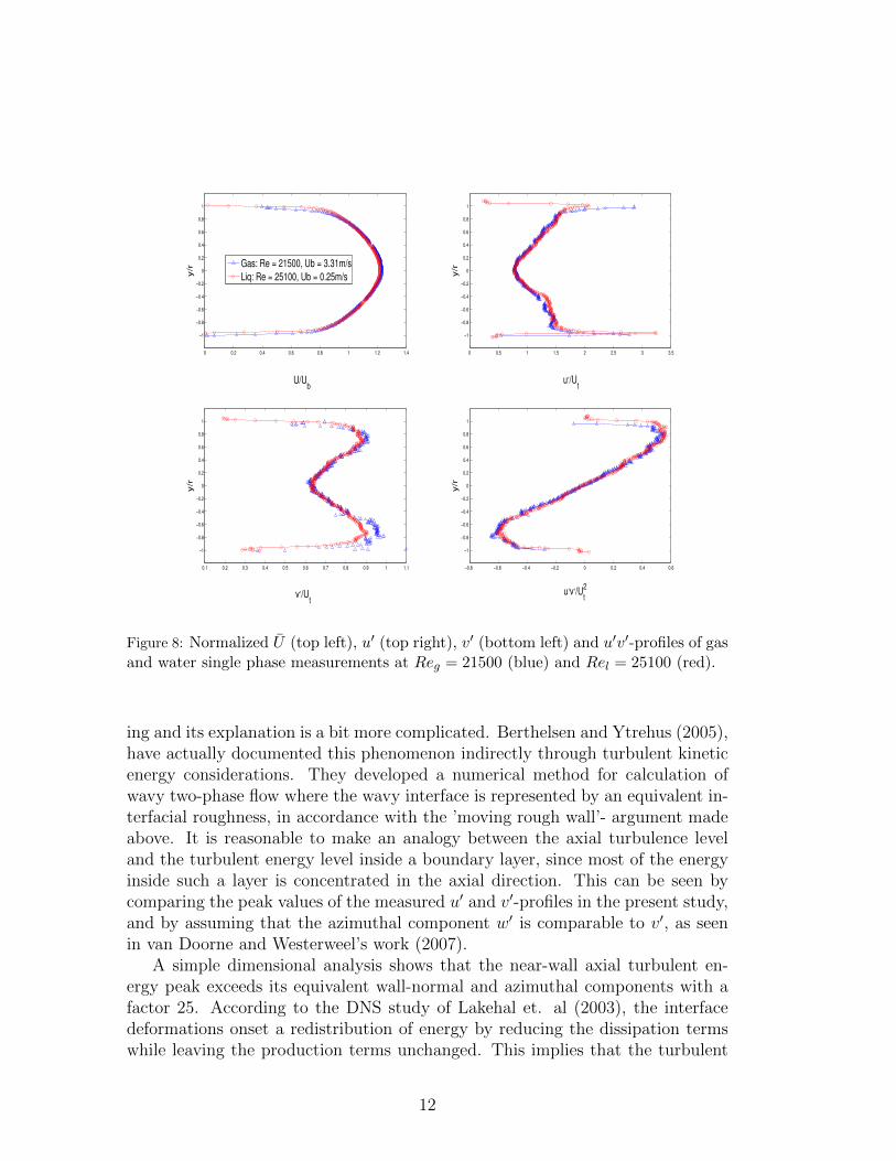
First order statistics of the gas single-phase, here Ug, compare perfectly withboth the DNS simulations and the Rel = 21500 liquid single phase experimentshown in Figure 8. The axial turbulence profiles also show satisfactory agreementin the main pipe region in both comparisons. However, close to the pipe walls,

9

the PIV peaks exceed the DNS peaks by roughly 50%. This can be due to eithermeasurement uncertainties related to levels of distortion near the pipe walls, oran under prediction in the DNS calculations. In the case of the first cause, theuncertainties should be of equal magnitude on both ends of the pipe. Thus, theratio between these peaks should reflect the nature of the flow, meaning thatfor a fully turbulent and symmetric flow, this ratio should be equal to 1. Thisis seen only in the ∆t = 112µs-case and Reg = 21500. The asymmetry seenin the ∆t = 65µs-case was actually caused by the water stream formed by theheavy tracer droplets, as explained earlier. The higher peak at the bottom isin accordance with the fact the water stream was wavy, and thus increased theroughness locally. This is actually a two-phase flow phenomenon and will bediscussed more in detail later in this paper. The water stream was partiallyavoided in the other gas single-phase case.

The asymmetry seen in the water case is reversed (top peak is lower thanbottom peak) and was caused by a totally different situation. Occasionally, elon-gated air bubbles occupied a very thin layer at the top wall and changed theboundary conditions locally, leading to free surface flow. Hence, the averagedaxial turbulence level was lower than in a pure single-phase flow.

It can be concluded from the presented single phase tests, that the PIV set-upwith its gas seeding technique provides very good measurements in both phases.The few deviations that have been observed are due to explainable circumstanceswhich, luckily, have no significance in two-phase flow experiments.

3. Two-Phase measurements

In this section a set of two stratified air/water flows are presented in terms ofthe vertical line mean and rms velocity profiles, in which the interface detectionmethod described earlier has been applied to obtain smooth profile transitionsbetween the phases, see Figure 9. The physical parameters that characterize theseexperiments are listed in the table with bold characters, see figure 2. The firstcase (red line) represents a stratified smooth flow, while the second case (greenline) represents a wavy flow. The waves were typical long 2D gravity waves withrelatively low amplitudes.

The U -profiles (top left plot) offer a global image of the flow characteristicsof both cases. They show that the gas flow rate was increased considerablywhile the liquid rate was lowered in order to obtain the desired wavy regime.However, the most interesting effects of this sub-regime change are definitelyseen in the turbulence profiles. In fact, a great deal of physics may be revealedjust by studying the near-wall and near-interface peaks, especially in the axialturbulence profiles.

In the smooth case, it is clear that the near-wall peak of the axial fluctuatinggas velocity u′g,wp

is larger than the near-interface u′g,ip peak. This feature is notsurprising and can be explained quite easily through the boundary conditions

10

−0.2 0 0.2 0.4 0.6 0.8 1 1.2 1.4

−1

−0.8

−0.6

−0.4

−0.2

0

0.2

0.4

0.6

0.8

1

U/Ub

y/r

0 0.5 1 1.5 2 2.5 3 3.5 4 4.5

−1

−0.8

−0.6

−0.4

−0.2

0

0.2

0.4

0.6

0.8

1

u’/Ut

y/r

0 0.2 0.4 0.6 0.8 1 1.2 1.4

−1

−0.8

−0.6

−0.4

−0.2

0

0.2

0.4

0.6

0.8

1

v’/Ut

y/r

−1 −0.8 −0.6 −0.4 −0.2 0 0.2 0.4 0.6 0.8 1

−1

−0.8

−0.6

−0.4

−0.2

0

0.2

0.4

0.6

0.8

1

u’v’/Ut2

y/r

Dt = 65 us, Ub = 6.74 m/s

Dt = 112us, Ub = 6.93 m/s

DNS

Figure 7: Normalized U (top left), u′ (top right), v′ (bottom left) and u′v′-profiles oftwo gas single phase PIV experiments at Reg = 44000 with ∆t = 65µs and 112µs arecompared to DNS data from Wu and Moin (2008).

that are imposed on the gas phase. Namely, no-slip condition both at a non-moving wall on one side, and a moving smooth interface on the other side. Thissituation is analogous to a turbulent couette flow in a semi-pipe with a movingbottom wall. The velocity gradient is much higher near the wall than near theinterface leading to a higher turbulence level.

Moreover, in the second case, where the flow is characterized by its wavy inter-face, a very different situation occurs. This time, the near-interface peak u′g,ip islarger than both its equivalent smooth case value and its corresponding near wallpeak u′g,wp

, which actually is lower than in the smooth case. Both observationsare direct consequences of the presence of waves. The enhancement at the inter-face is easily explained by the fact that, in a time-averaged sense, the gas phaseperceives the wavy interface as a moving wall with a considerable roughness.Higher roughness leads inevitably to thicker and more turbulent boundary-layernear the interface.

However, the latter observation (drop near the wall) may seem rather surpris-

11

0 0.2 0.4 0.6 0.8 1 1.2 1.4

−1

−0.8

−0.6

−0.4

−0.2

0

0.2

0.4

0.6

0.8

1

U/Ub

y/r

0 0.5 1 1.5 2 2.5 3 3.5

−1

−0.8

−0.6

−0.4

−0.2

0

0.2

0.4

0.6

0.8

1

u,/U

t

y/r

0.1 0.2 0.3 0.4 0.5 0.6 0.7 0.8 0.9 1 1.1

−1

−0.8

−0.6

−0.4

−0.2

0

0.2

0.4

0.6

0.8

1

v,/U

t

y/r

−0.8 −0.6 −0.4 −0.2 0 0.2 0.4 0.6

−1

−0.8

−0.6

−0.4

−0.2

0

0.2

0.4

0.6

0.8

1

u,v

,/U

t

2

y/r

Gas: Re = 21500, Ub = 3.31m/s

Liq: Re = 25100, Ub = 0.25m/s

Figure 8: Normalized U (top left), u′ (top right), v′ (bottom left) and u′v′-profiles of gasand water single phase measurements at Reg = 21500 (blue) and Rel = 25100 (red).

ing and its explanation is a bit more complicated. Berthelsen and Ytrehus (2005),have actually documented this phenomenon indirectly through turbulent kineticenergy considerations. They developed a numerical method for calculation ofwavy two-phase flow where the wavy interface is represented by an equivalent in-terfacial roughness, in accordance with the ’moving rough wall’- argument madeabove. It is reasonable to make an analogy between the axial turbulence leveland the turbulent energy level inside a boundary layer, since most of the energyinside such a layer is concentrated in the axial direction. This can be seen bycomparing the peak values of the measured u′ and v′-profiles in the present study,and by assuming that the azimuthal component w′ is comparable to v′, as seenin van Doorne and Westerweel’s work (2007).

A simple dimensional analysis shows that the near-wall axial turbulent en-ergy peak exceeds its equivalent wall-normal and azimuthal components with afactor 25. According to the DNS study of Lakehal et. al (2003), the interfacedeformations onset a redistribution of energy by reducing the dissipation termswhile leaving the production terms unchanged. This implies that the turbulent

12

activity persists near the interface, which is confirmed by this study.An alternative explanation of the physics that lie behind the reduction of

the wall axial turbulence may be obtained by considering the following thoughtexperiment: It is of common knowledge that the onset of waves in a gas-liquid flowis caused by an instability or a perturbation at the interface that grows with timeuntil it reaches a stable wavy state which is maintained by the kinetic energy ofthe gas phase. Theoretically, one could prevent such instabilities from occurringsuch that the interface would remain smooth even at gas flow rates that normallywould generate a waves.This could be achieved in a perfectly round, smooth andhorizontal pipe which is isolated from all temperature and pressure changes andin which both the gas and liquid flows are perfectly isotropic and homogeneous.Obviously, these conditions are rather impossible to attain in a laboratory.

Another important feature of stratified gas-liquid pipe flow that must be re-called, is that the turbulent energy production is mainly concentrated inside theviscous boundary layers near the wall and the interface. In the special case of asmooth interface flow, it can be argued that production rate is higher inside thewall boundary layer than in the interfacial boundary layer since the stream wisevelocity gradient is lower there.

Now, by introducing a perturbation to the interface, the flow would quicklystabilize into a wavy regime with characteristics conformed by the kinetic energythat already exists in the gas phase. Considering this case in a time-averagedsense, the ’moving rough wall’- analogy of the interface would imply higher turbu-lent energy production rate in the interfacial boundary. Since no external energywas added to the system, a redistribution of energy must take place in the re-maining pipe region, including the wall region. This is in agreement with boththe drop seen in figure 9 and Lakehal’s conclusion (2003).

Furthermore, a dramatic enhancement of the liquid wall-normal turbulentcomponent v′l is seen in the wavy case. Qualitatively, this observation is not sur-prising. However, extra care is needed when evaluating this result quantitatively.It should be remarked that the oscillatory motion of the waves must have had aninfluence on the computation of the v-rms profile. One wayto deal with this chal-lenge, is to subtract the oscillations due to the waves from the raw wall-normalvelocity profile before computing the rms.

These qualitative results confirm many already known aspects of the turbu-lence structure in stratified gas/liquid two-phase flow and offer a motivation forfurther investigation.

3.1. Streamwise Turbulence Analysis

A set of 17 stratified air-water flow experiments of varying flow rates wereconducted using the PIV set-up described earlier. Measured physical and flowproperties such as the liquid hold-up HL, the gas pressure drop ∆Pg

L, the gas and

liquid Re-numbers (both superficial and hydraulic), the mean and superficial ve-locities, Ub,f and Usf and finally, the axial gas turbulence profiles are investigated

13

−0.5 0 0.5 1 1.5 2 2.5 3 3.5

−1

−0.8

−0.6

−0.4

−0.2

0

0.2

0.4

0.6

0.8

1

m/s

y/r

Umean

0 0.1 0.2 0.3 0.4 0.5 0.6 0.7

−1

−0.8

−0.6

−0.4

−0.2

0

0.2

0.4

0.6

0.8

1

Urms

m/s

y/r

0 0.02 0.04 0.06 0.08 0.1 0.12 0.14

−1

−0.8

−0.6

−0.4

−0.2

0

0.2

0.4

0.6

0.8

1

Vrms

m/s

y/r

−8 −6 −4 −2 0 2 4 6 8 10

x 10−3

−1

−0.8

−0.6

−0.4

−0.2

0

0.2

0.4

0.6

0.8

1

uv

[m/s]2

y/r

Gphase: Usg = 0.70 m/s

Lphase: Usl = 0.08 m/s

Gphase: Usg = 1.26 m/s

Lphase: Usl = 0.04 m/s

Figure 9: Mean axial profile U (upper left), axial (upper right) and vertical (lower left)fluctuating velocity profiles u′ and v′ and finally Re-stress profile u′v′ for a flat smoothinterface (red) and wavy interface (green). The thick lines indicate measurements inthe water-phase.

further. The focus of this study is limited to the axial turbulence, partially be-cause a great deal of consistency was found in all u′-profiles, confirming the highdegree of accuracy in second order statistics in this direction, and also becausethe shape of the profiles looked to cohere with the nature of the interface, as seenin figure 10, hinting about the existence of a correlation between them. Hence,the aim of this study is to search for such a correlation, at least qualitatively.The table in figure 2 contains the physical parameters of each experiment, whilefigure 3 displays their liquid hold-ups.

Different flow patterns were identified visually while performing the exper-iments and these were found to match the descriptions provided by Espedal(1998), Strand (1993) and Fernandino and Ytrehus (2006). Espedal and Strandused wave probes inside their pipes, respectively 100 mm and 60 mm i.d., and an-alyzed the cross correlation values in order to quantify the various wave patterns.Espedal divided them into the following 5 different regions:

1. Smooth flow: No waves were observed.

14

Figure 10: PIV images of a smooth, rippled and wavy flow shown with their belonging(time-averaged) axial turbulence profiles.

2. Small amplitude waves I: Amplitudes below 2 mm and wave lengths between2 and 6 cm. The power spectrum showed no peak at all or one peak.

3. Small amplitude 2D waves II: Similar to the waves above, but the powerspectrum showed two peaks.

4. Large amplitude 2D waves: Amplitudes above 2 mm, and the waves areless regular. The power spectrum has a one, two or no marked peaks.

5. Large amplitude 3D waves: Amplitudes above 2 mm, and the waves do nothave a two dimensional shape.

Ytrehus and Fernandino (2006) used the laser doppler velocimetry (LDV)technique to measure the fluctuations that occur close to the air-sheared interface.By analyzing the spectra of the LDV signal, they emphasized that intermediatepatterns exist between the well defined ones. Espedal’s identifications up tothe ”small amplitude 2D waves II” were found to agree very well with the flowpatterns that were observed during this study. However, the second sub-regime isreferred to as ”rippled flow” and is believed to consist of capillary waves riding on

15

top of an otherwise flat interface. The rippled flow shares some common featureswith the smooth flow in regard to the turbulence structure. This is discussed inmore details later.

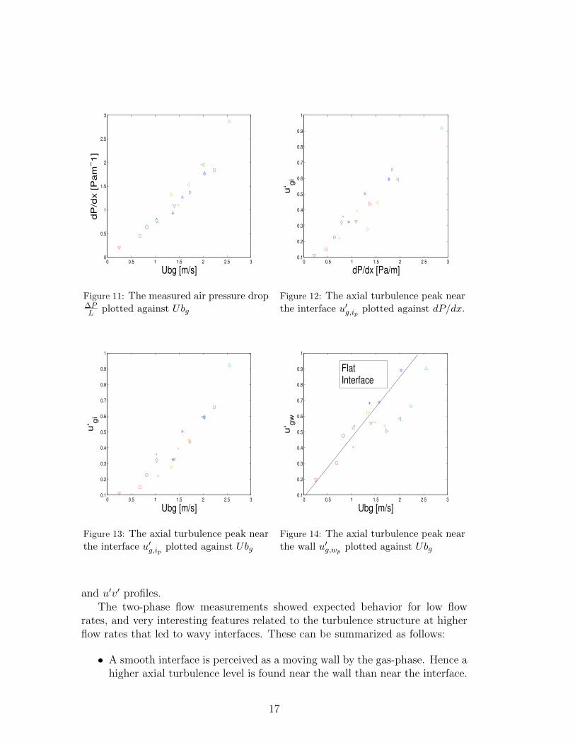
Figure 11 shows the measured gas pressure drops of each experiment plottedwith their corresponding mean local velocities Ubg. There seems to be a linearrelationship between them, at least for the relatively low pressure region in whichthe present experiments operate. Strand (1993) claimed that the pressure dropincreases almost quadratically with respect to the gas flow rate for fixed liquidrates. But, this does not have to contradict the present results, since he studiedflows with significantly higher pressure drops.

One of the most important results of this study is seen in figure 12, wherethe near interface peak value of the axial turbulence, ug,ip , is plotted against thepressure drop. Here, a very similar linear correlation is found as in figure 11. Thisresult indicates that the same relationship should be expected also between ug,ipand Ubg. This is seen in figure 13. This means that changes in the local meanvelocity affect the pressure drop and the interfacial axial turbulence analogously.

Furthermore, figure 14 shows that in the smooth and rippled interface cases(generalized by the term ”flat”), the wall turbulence also follows a linear evolutionwith respect to increasing Ubg. However, a drop from this linear trend is presentin all non-flat cases, confirming the qualitative observations made in the previoussection. This result explains the choice of the term ”rippled” instead of smallamplitude 2D waves as denoted by Espedal. The capillary waves have very smallamplitudes, and the interface deformations that they cause are not sufficientlylarge for a redistribution of energy to occur.

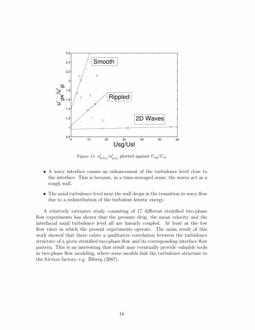
Finally, the main result of this paper is presented in figure 15. Here the

ratio between the wall and interface turbulence peaksu′g,wp

u′g ,ipis plotted against the

superficial velocity ratio Usg

Usl. A clear distribution of three linear trends arise in

accordance to the observed flow patterns, smooth, rippled and small amplitude2D waves. Some intermediate cases are also visible between the linear trends.This is in agreement with Fernandino’s (2006) conclusions. This result provesthat the turbulence structure of any stratified gas-liquid flow is characterized byits actual interface behavior.

4. Concluding remarks

Simultaneous PIV measurements of stratified gas/liquid two-phase flow in ahorizontal pipe have been successfully performed using water droplets, 1− 5µmin diameter as tracers in the gas phase. Single phase experiments have beenconducted for the sake of validation of the seeding technique and the experimentalset-up. The results from these have been compared to DNS results and to liquidsingle phase experiments showing perfect agreement in the first order statistics,i.e. U -profile, and satisfactory agreement in the second order statistics, i.e. u′, v′

16

0 0.5 1 1.5 2 2.5 30

0.5

1

1.5

2

2.5

3

Ubg [m/s]

dP

/dx [P

am

−1]

Figure 11: The measured air pressure drop∆PL plotted against Ubg

0 0.5 1 1.5 2 2.5 30.1

0.2

0.3

0.4

0.5

0.6

0.7

0.8

0.9

1

dP/dx [Pa/m]

u‘ g

iFigure 12: The axial turbulence peak nearthe interface u′g,ip plotted against dP/dx.

0 0.5 1 1.5 2 2.5 30.1

0.2

0.3

0.4

0.5

0.6

0.7

0.8

0.9

1

Ubg [m/s]

u‘ g

i

Figure 13: The axial turbulence peak nearthe interface u′g,ip plotted against Ubg

0 0.5 1 1.5 2 2.5 30.1

0.2

0.3

0.4

0.5

0.6

0.7

0.8

0.9

1

Ubg [m/s]

u‘ g

w

FlatInterface

Figure 14: The axial turbulence peak nearthe wall u′g,wp

plotted against Ubg

and u′v′ profiles.The two-phase flow measurements showed expected behavior for low flow

rates, and very interesting features related to the turbulence structure at higherflow rates that led to wavy interfaces. These can be summarized as follows:

• A smooth interface is perceived as a moving wall by the gas-phase. Hence ahigher axial turbulence level is found near the wall than near the interface.

17

0 10 20 30 40 50 600.8

1

1.2

1.4

1.6

1.8

2

2.2

2.4

2.6

Usg/Usl

u‘ g

w/u

‘ gi

Smooth

Rippled

2D Waves

Figure 15: u′g,wp/u′g,ip plotted against Usg/Usl

• A wavy interface causes an enhancement of the turbulence level close tothe interface. This is because, in a time-averaged sense, the waves act as arough wall.

• The axial turbulence level near the wall drops in the transition to wavy flowdue to a redistribution of the turbulent kinetic energy.

A relatively extensive study consisting of 17 different stratified two-phaseflow experiments has shown that the pressure drop, the mean velocity and theinterfacial axial turbulence level all are linearly coupled. At least at the lowflow rates in which the present experiments operate. The main result of thiswork showed that there exists a qualitative correlation between the turbulencestructure of a given stratified two-phase flow and its corresponding interface flowpattern. This is an interesting that result may eventually provide valuable toolsin two-phase flow modeling, where some models link the turbulence structure tothe friction factors, e.g. Biberg (2007).

18

[1] Andreussi, P. and Persen, LN. Stratified gas-liquid flow in downwardly in-clined pipes. I.J. of Multiphase Flow, 13:565-575, 1986.

[2] Andritsos, N. and Hanratty, T.J. Influence of interfacial waves in stratifiedgas-liquid flows. AIChE Journal, 33:444-454, 1987.

[3] Berthelsen, P.A. and Ytrehus, T. Calculations of stratified wavy two-phaseflow in pipes. I.J. of Multiphase Flow , 31:571-592, 2005.

[4] Biberg, D. A Mathematical Model For Two-Phase Stratified Turbulent DuctFlow. Multiphase Science and Technology, 19:1-48, 2007.

[5] Carpintero-Rogerol, E., Kross, B. and Sattelmayer, T. Simultaneous HS-PIVand shadowgraph measurements of gas-liquid flows in a horizontal pipe. 13thInt. Symp. on Applications of Laser Techniques to Fluid Mechanics, 2006.

[6] Espedal, M. An experimental investigation of stratified two-phase pipe flowat small inclinations. PhD Thesis, The Norwegian University of Science andTechnology (NTNU), 1998.

[7] Fernandino, M. and Ytrehus, T. Determination of flow sub-regimes in strat-ified air-water channel flow using LDV spectra. I.J of Multiphase Flow,32:436-446, 2006.

[8] Fabre, J., Masbernat, L. and Suzanne, C. Stratified flow, Part I: local struc-ture. Multiphase Science and Technology, 3:285-301, 1987.

[9] Johnson, J.W. PhD Thesis - A study of stratified gas-liquid pipe flow. Uni-versity of Oslo, 2005.

[10] Kumara, W.A.S. PhD Thesis - An Experimental Study of Oil-Water Flowin Pipes. Telemark University College, 2010.

[11] Lakehal, D., Fulgosi, M. and Banerjee, S. and De Angelis. Direct NnumericalSimulation of Turbulence in a Sheared Air Water Flow With a DeformableInterface. J. Fluid Mech, 482:319-345, 2003.

[12] Lorencez, C, Nasr-Esfahany, M., Kawaji, M. and Ojha, M. Liquid turbulencestructure at a sheared and wavy gasliquid interface. Int. J. Multiphase Flow,23:205-226, 1997.

[13] Melling, A. Tracer Particles and Seeding for Particle Image Velocimetry.Measurement Science and Technology, 8:1406-1416, 1997.

[14] Mokhatab, S., Poe, W and Speight, J.G. Handbook of Natural Gas Trans-mission and Processing. 2006.

19

[15] Sanchis, A. and Jensen, A. Dynamic Masking of PIV Images Using theRadon Transform in Free Surface Flows. Exp. in Fluids,51:871-880, 2011.

[16] Sanchis, A., Johnson, G. and Jensen, A. The formation of hydrodynamicslugs by the interaction of waves in gas-liquid two-phase pipe flow. I.J. ofMultiphase Flow, 37:358-368, 2011.

[17] Schulkes, R. An Introduction to Multiphase Pipe Flow. University of Oslo,2010.

[18] Strand, O. An experimental investigation of stratified two-phase flow inhorizontal pipes. PhD Thesis, University of Oslo, 1993.

[19] Sveen, J. and Cowen, E.A. Quantitative Imaging Techniques and Their Ap-plication to Wavy Flows. Suranaree University of Technology, 2004.

[20] Ullmann, A. and Brauner, N. Closure relations for two-fluid models for two-phase stratified smooth and stratified wavy flows. I.J. of Multiphase Flow ,32:81-112, 2006.

[21] van Doorne, C.W.H. and Westerweel, J. Measurement of laminar, transi-tional and turbulent pipe flow using Stereoscopic-PIV. Exp Fluids, 42:259-279, 2007.

[22] Westerweel, J. Fundamentals of Digital Particle Image Velocimetry. Mea-surement Science and Technology, 8:1379-1392, 2008.

[23] Wu, X. and Moin, P. A Direct Numerical Simulation Study on the MeanVelocity Characteristics in Turbulent Pipe Flow. J. Fluid Mech, 608:81-112,2008.

20