HAL Id: hal-01510186https://hal.archives-ouvertes.fr/hal-01510186

Submitted on 19 Apr 2017

HAL is a multi-disciplinary open accessarchive for the deposit and dissemination of sci-entific research documents, whether they are pub-lished or not. The documents may come fromteaching and research institutions in France orabroad, or from public or private research centers.

L’archive ouverte pluridisciplinaire HAL, estdestinée au dépôt et à la diffusion de documentsscientifiques de niveau recherche, publiés ou non,émanant des établissements d’enseignement et derecherche français ou étrangers, des laboratoirespublics ou privés.

Pitch-Axis Identification for a Guided Projectile Using aWind-Tunnel-Based Experimental Setup

Guillaume Strub, Simona Dobre, Vincent Gassmann, Spilios Theodoulis,Michel Basset

To cite this version:Guillaume Strub, Simona Dobre, Vincent Gassmann, Spilios Theodoulis, Michel Basset. Pitch-AxisIdentification for a Guided Projectile Using a Wind-Tunnel-Based Experimental Setup. IEEE/ASMETransactions on Mechatronics, Institute of Electrical and Electronics Engineers, 2016, 21 (3), pp.1357-1365. �10.1109/TMECH.2016.2525719�. �hal-01510186�

1

Pitch Axis Identification for a Guided Projectileusing a Wind Tunnel-based Experimental Setup

Guillaume Strub1,2, Simona Dobre1, Vincent Gassmann1, Spilios Theodoulis1, Michel Basset2

Abstract—This article details the identification of a pitchaxis model for an 80mm fin-stabilized, canard-guided projec-tile through a Hardware-in-the-Loop experimental setup. Thissetup is based on an autonomous functional projectile prototypeinstalled in a subsonic wind tunnel by the means of a 3 Degreesof Freedom (DoF) gimbal mount. A nonlinear dynamical modelis first derived from flight mechanics principles, then a linearizedmodel is obtained through Taylor series expansion. The a prioriand a posteriori identifiability of the proposed linear modelare assessed and the associated experimental input signals areaccordingly designed. The model parameters are then estimatedusing a numerical optimization procedure and the associateduncertainty is obtained through a boostrapping method. Theresults and their implication on the projectile flight control designare finally discussed.

Index Terms—Guided Projectiles, Flight Mechanics, SystemsIdentification, Uncertain Systems

I. INTRODUCTION

THE interest in guided projectile concepts has grownsteadily over the last decades. Indeed, they can vastly

improve precision and range over traditional ballistic ammu-nition [1], [2]. The latter typically exhibit poor performancedue to their sensitivity to initial launch conditions and theirinability to reject in-flight disturbances. However, they remainsignificantly less expensive than missile systems, which em-ploy high-performance actuators and sensors as well as sophis-ticated guidance, navigation and control (GNC) algorithms.The key idea in guided projectile design is to develop missile-like GNC functionality using low-cost, g-hardened actuators,sensors and embedded processors.

The projectile flight control laws are at the core of the GNCalgorithms and deal with platform stabilization, disturbancerejection and reference tracking. The design of these controllaws is mostly done through model-based control techniques[3], [4], hence the need for an accurate projectile dynamicmodel. Projectiles and missiles obey the principles of flightmechanics, which describe the rigid body dynamic and kine-matic behavior [5]. This behavior is characterized by theaerodynamic forces and moments, which cannot be analyt-ically computed. Several methods are able to quantify theaerodynamic coefficients of projectiles. In that respect, basic

*This work is in part financed by the French Defense Procurement Agency(DGA, Direction Generale de l’Armement)

1G. Strub, S. Dobre, V. Gassmann and S. Theodoulis are with the French-German research Institute of Saint-Louis (ISL), 5 rue du General Cassagnou,68301 Saint-Louis, France. E-mail: guillaume.strub@isl.eu

2G. Strub and M. Basset are with the Modeling, Intelligence, Processand Systems (MIPS) Laboratory EA2332, 12 rue des Freres Lumiere, 68093Mulhouse, France

information is generally gathered through Computational FluidDynamics (CFD) analysis [6], empirical or semi-empiricalcodes like PRODAS (PROjectile Design/Analysis System) [7]or Missile DATCOM [8], wind tunnel tests [9] and/or free-flight experiments [10].

In this work we present an additional technique based on afunctional autonomous projectile prototype installed in a windtunnel, by means of a support allowing rotation around allaxes (Roll, Pitch and Yaw). The model parameters, describingthe behavior of the projectile in flight, can be estimated by themeans of system identification and wind-tunnel experimentaldata. As the input signals can be fully specified, this techniqueleads to better excitation and conditioning than free-flightidentification, in which the input can be difficult to modify inflight. The proposed setup is also applicable to control studiesand especially controller validation through real-time testing.

The proposed approach is akin to Hardware-In-the-Loopsimulation, which is used in various fields such as robotics,automotive or aerospace design and consists in includinghardware components in a simulation loop [11]. One typicalHIL use case is the simulation of a part of a system whichmay not be available or can be difficult to implement in anexperimental setup. For example in Verma et al. [12], thedynamics of a high-mobility multipurpose wheeled vehicle aresimulated using a scaled-down model in a HIL simulation,where the ultimate goal is to build a collision avoidancealgorithm testbed. In our case, the projectile free-flight be-havior is difficult to exploit, therefore it is emulated usingthe controlled environment provided by the wind tunnel andsupport structure.

To the authors’ best knowledge, there are few similar setupsfor identification and control investigation on guided projec-tiles. In Hann et al. the roll dynamics of a sounding rocket in avertical wind tunnel are analyzed through a minimal modelingapproach and integral-based parameter identification. Fresconiet al. [13] propose a projectile prototype using a similar low-cost maneuver system, where a roll controller using linearquadratic optimal control and a PRODAS-derived model isdesigned and assessed in terms of performance. In both cases,only the roll axis is considered, whereas the proposed setupenables simultaneous rotation on the pitch, roll and yaw axes.

The present article focuses on the identification of a control-oriented pitch axis model. Using flight mechanics principles,a nonlinear dynamic model is constructed and linearized foroperation around equilibrium points. A complete identificationstudy is then conducted. First, the identifiability of the pro-posed linear model parameters is assessed. An optimal inputsignal is then built using this knowledge, and the projectile is

2

excited around several equilibrium points. Finally, the linearmodel parameters and associated uncertainties are estimatedfrom the collected experimental data.

This paper is structured as follows: Section II describes theACHILES experimental setup. In Section III, the projectilepitch axis model is derived from flight mechanics principles.Section IV deals with the identifiability and estimation of theproposed model. The results and their implication on flightcontrol design are discussed in Section V.

II. EXPERIMENTAL SETUP

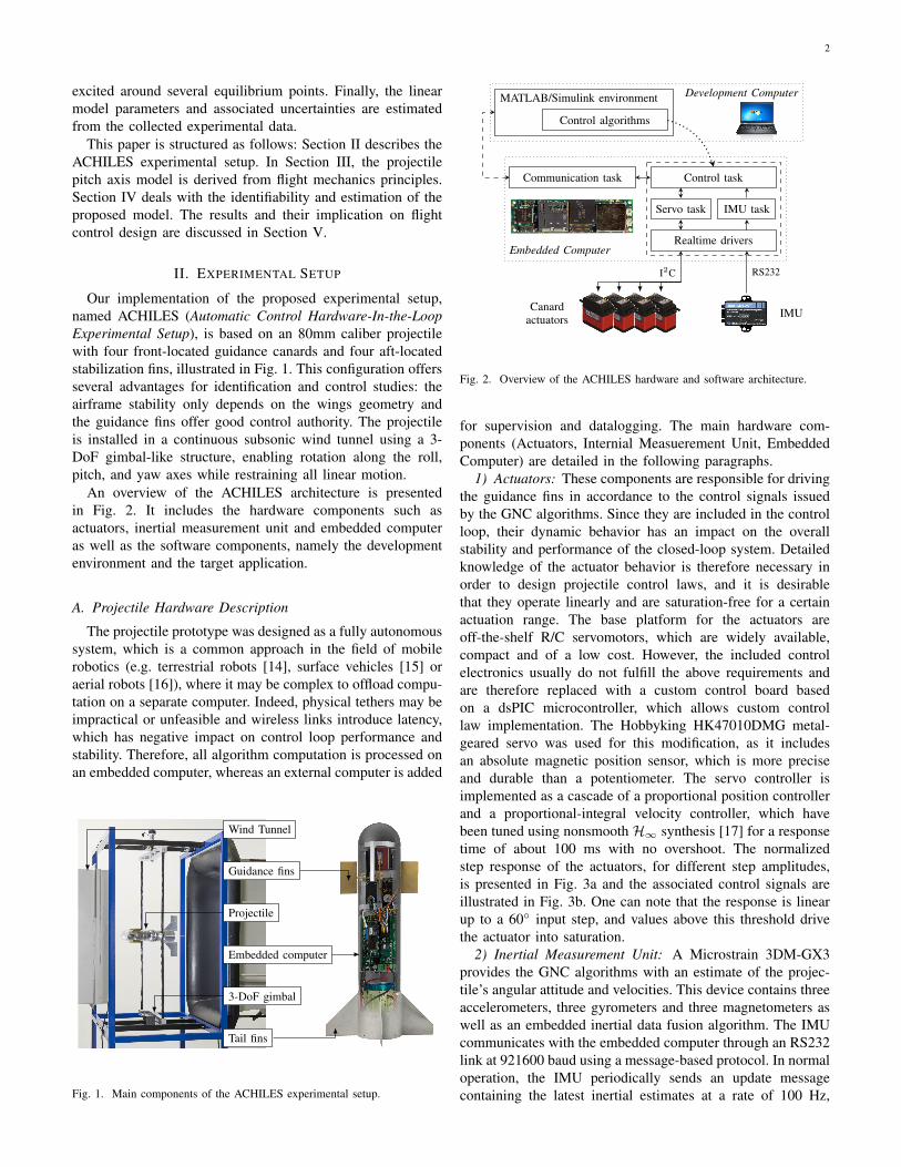
Our implementation of the proposed experimental setup,named ACHILES (Automatic Control Hardware-In-the-LoopExperimental Setup), is based on an 80mm caliber projectilewith four front-located guidance canards and four aft-locatedstabilization fins, illustrated in Fig. 1. This configuration offersseveral advantages for identification and control studies: theairframe stability only depends on the wings geometry andthe guidance fins offer good control authority. The projectileis installed in a continuous subsonic wind tunnel using a 3-DoF gimbal-like structure, enabling rotation along the roll,pitch, and yaw axes while restraining all linear motion.

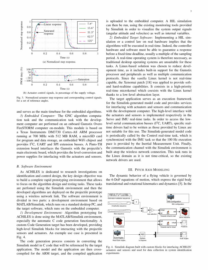
An overview of the ACHILES architecture is presentedin Fig. 2. It includes the hardware components such asactuators, inertial measurement unit and embedded computeras well as the software components, namely the developmentenvironment and the target application.

A. Projectile Hardware Description

The projectile prototype was designed as a fully autonomoussystem, which is a common approach in the field of mobilerobotics (e.g. terrestrial robots [14], surface vehicles [15] oraerial robots [16]), where it may be complex to offload compu-tation on a separate computer. Indeed, physical tethers may beimpractical or unfeasible and wireless links introduce latency,which has negative impact on control loop performance andstability. Therefore, all algorithm computation is processed onan embedded computer, whereas an external computer is added

Wind Tunnel

Guidance fins

3-DoF gimbal

Tail fins

Projectile

Embedded computer

Fig. 1. Main components of the ACHILES experimental setup.

Development ComputerMATLAB/Simulink environment

Control algorithms

Embedded Computer

Control task

Servo task IMU task

Realtime drivers

RS232

IMU

I2C

Canardactuators

Communication task

Fig. 2. Overview of the ACHILES hardware and software architecture.

for supervision and datalogging. The main hardware com-ponents (Actuators, Internial Measuerement Unit, EmbeddedComputer) are detailed in the following paragraphs.

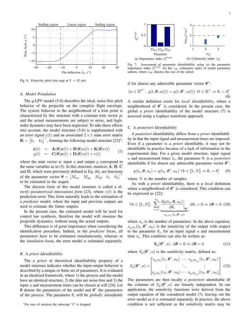
1) Actuators: These components are responsible for drivingthe guidance fins in accordance to the control signals issuedby the GNC algorithms. Since they are included in the controlloop, their dynamic behavior has an impact on the overallstability and performance of the closed-loop system. Detailedknowledge of the actuator behavior is therefore necessary inorder to design projectile control laws, and it is desirablethat they operate linearly and are saturation-free for a certainactuation range. The base platform for the actuators areoff-the-shelf R/C servomotors, which are widely available,compact and of a low cost. However, the included controlelectronics usually do not fulfill the above requirements andare therefore replaced with a custom control board basedon a dsPIC microcontroller, which allows custom controllaw implementation. The Hobbyking HK47010DMG metal-geared servo was used for this modification, as it includesan absolute magnetic position sensor, which is more preciseand durable than a potentiometer. The servo controller isimplemented as a cascade of a proportional position controllerand a proportional-integral velocity controller, which havebeen tuned using nonsmooth H∞ synthesis [17] for a responsetime of about 100 ms with no overshoot. The normalizedstep response of the actuators, for different step amplitudes,is presented in Fig. 3a and the associated control signals areillustrated in Fig. 3b. One can note that the response is linearup to a 60◦ input step, and values above this threshold drivethe actuator into saturation.

2) Inertial Measurement Unit: A Microstrain 3DM-GX3provides the GNC algorithms with an estimate of the projec-tile’s angular attitude and velocities. This device contains threeaccelerometers, three gyrometers and three magnetometers aswell as an embedded inertial data fusion algorithm. The IMUcommunicates with the embedded computer through an RS232link at 921600 baud using a message-based protocol. In normaloperation, the IMU periodically sends an update messagecontaining the latest inertial estimates at a rate of 100 Hz,

3

125◦

62.5◦

31.3◦

15.6◦

7.8◦

No

rmal

ized

step

resp

on

se

Time (s)

Saturatedresponse

Linear response

0 0.2 0.4 0.6 0.8 1

0

0.2

0.4

0.6

0.8

1

(a) Normalized step response.

PW

Md

uty

(%)

Time (s)

Saturation

0 0.2 0.4 0.6 0.8 1

−100

−50

0

50

100

(b) Actuator control signals, in percentage of the supply voltage.

Fig. 3. Normalized actuator step response and corresponding control signals,for a set of reference angles.

and serves as the main timebase for the embedded algorithms.3) Embedded Computer: The GNC algorithm computa-

tion task and the communication task with the develop-ment computer are performed on an onboard Gumstix OveroFireSTORM computer on-module. This module is based ona Texas Instruments DM3730 Cortex-A8 ARM processorrunning at 700 MHz with 512 MB RAM, a microSD cardfor program and data storage, an embedded WiFi chipset andprovides I2C, UART and SPI extension busses. A Pinto-THextension board interfaces the Gumstix with the projectile’smain electronic board, which provides the level-conversion andpower supplies for interfacing with the actuators and sensors.

B. Software Environment

As ACHILES is dedicated to research investigations onidentification and control design, the key design objective wasto build a complete rapid prototyping environment that allowsto focus on the algorithm design and testing tasks. These tasksare perfomed using the Simulink environment and then thedeveloped algorithms are deployed on the projectile prototypeusing a wireless network link. The software environment isdivided in two parts: a development environment based onMATLAB/Simulink, which runs on a standard desktop PC, andthe target software, which runs on the embedded computer.

1) Development Environment: Algorithm prototyping forACHILES is done using the MATLAB/Simulink environment,especially the automatic C code generation functionality. Acustom Code Generation target has been developed, providinghigh-level Simulink blocks for interacting with the projectilesensors and actuators. An exemple use case is presented inFig. 4.

The code generation process consists in converting theSimulink model in C code that will be referenced by the targetapplication. The model and the application are then cross-compiled for the ARM target, and the compiled application

is uploaded to the embedded computer. A HIL simulationcan then be run, using the existing monitoring tools providedby Simulink in order to visualize the system output signals(angular attitude and velocites) as well as internal variables.

2) Embedded Target Software: Implementing a HIL sim-ulation or a control law on real hardware implies that thealgorithms will be executed in real-time. Indeed, the controllerhardware and software must be able to guarantee a responsebefore a fixed time deadline, usually a multiple of the samplingperiod. A real-time operating system is therefore necessary, astraditional desktop operating systems are unsuitable for thesetasks. A Linux-based solution was chosen to reduce devel-opment time, as it includes built-in support for the Gumstixprocessor and peripherals as well as multiple communicationprotocols. Since the vanilla Linux kernel is not real-timecapable, the Xenomai patch [18] was applied to provide soft-and hard-realtime capabilities. It consists in a high-priorityreal-time microkernel which coexists with the Linux kernelthanks to a low-level abstraction layer.

The target application serves as an execution frameworkfor the Simulink-generated model code and provides servicesfor interfacing with actuators and sensors and communicationwith the development computer. The high-level interface withthe actuators and sensors is implemented respectively in theServo and IMU real-time tasks. In order to access the low-level serial communication busses (I2C, UART), specific real-time drivers had to be written as those provided by Linux arenot suitable for this use. The Simulink-generated model codeis periodically called by the Control real-time task, which issynchronized with the IMU task so that the 100 Hz executionpace is provided by the Inertial Measurement Unit. Finally,the communication channel with the Simulink environment isbuilt atop the wireless network connection. This task runs inthe Linux domain as it is not time-critical, so the existingnetwork drivers are used.

III. PITCH AXIS MODELING

The dynamic behavior of a flying vehicle is governed bythe 6-DoF equations of motion, which express the rigid bodytranslational and rotational kinematics and dynamics [5]. In the

Euler AnglesRead Euler angles

Servo setpoints

Euler angles

Servo positions Positions

virtualroll real

fcnCanards virtual to real

-K-Axis selection

Estimation+validation sequences

Amplitudes sequence

Bias sequence

IMU ConfigurationIMU configuration

realroll virtual

fcnCanards real to virtual

R2DRadians

to Degrees

Fig. 4. Simulink diagram built with custom blocks for interfacing ACHILES’actuators and sensors and used for data collection in system identificationexperiments

4

ACHILES setup, the projectile is held at its center of gravityby the 3-DoF support structure, thereby preventing all linearmotion. This paper focuses on the pitch axis, and it is assumedthat no motion will occur on the roll and yaw axes, which canbe physically locked.

Figure 5 represents the projectile pitching motion and theassociated parameters, which are the angle of attack α, thebody pitch rate q and the fin deflection angle δm. The angleof attack is defined as the angle between the wind direction1W and the projectile longitudinal axis 1B, which is also equalto the pitch angle θ in the proposed configuration. The findeflection angle is relative to the body, with the sign takenso that a positive increment in δm induces a positive pitchingcontrol moment on the projectile body. This control signal isequally distributed over the four canards δ1 · · · δ4 such thatthey act as a single virtual pitch canard plane.

A. Nonlinear Model Derivation

The projectile pitch attitude equations are expressed usingthe flight mechanics framework [5]. Knowing that herein theobjective is to focus on the pitch axis identification, it will beassumed in the following part that the roll and yaw axes arelocked. Thus, the only motion left is about the 2B axis and thepitch dynamic and kinematic differential equations correspondto the application of Euler’s law to a planar body rotating aboutits center of gravity:

q = I−12 qSdCm(α,M)

α = q(1)

where I2 is the projectile inertia along the pitch axis 2B andqSdCm(α,M) corresponds to the pitching moment, whereCm is the total pitch moment aerodynamic coefficient. Otherquantities are the projectile reference area S, the caliber dand the dynamic pressure q = 1

2ρ(h)V 2, where ρ(h) is thealtitude-dependent air density. Here, h is constant (groundlevel) and V is the airspeed in the wind tunnel. The totalpitch aerodynamic coefficient can be decomposed as [5]:

Cm(α,M) =

Cmα(α,M)α+

(d

2V

)Cmq(M)q + Cmδ(α,M)δm (2)

where the aerodynamic derivatives Cmα, Cmq and Cmδ areunknown nonlinear functions of the Mach numberM and theangle of attack α and correspond to the partial derivatives ofCm with respect to α, q and δm. The Mach number is definedas M = V

a(h) where a(h) is the speed of sound at altitude h.At sea level, a = 343 m/s for a temperature of 20◦C and apressure of 1.013 bar.

B. Linearization and Trimming

Equations (1) and (2) form a nonlinear, parameter-dependent(NLPD) state-space model of the form:

x(t) = fx[x(t), u(t),σ(t)]y(t) = fy[x(t), u(t),σ(t)]

(3)

with x =[α q

]>being the state vector, u = δm the control

input and σ =[V h

]>an external parameter vector. The

measured output y of this system is the angle of attack α.This system can be linearized using a first-order Taylor

series expansion [19] around any equilibrium flight condition(x, u, σ) called trim point [20]. At the trim condition, the statederivative is by definition:

˙x , 0 = fx(x, u, σ) (4)

The projectile’s equilibrium manifold, or trim map, is de-termined experimentally by measuring the steady-state angleof attack for different fin deflection angles for fixed airspeed.The obtained trim map is represented in Fig. 6 and exhibitsa linear flight domain for δm ∈ [−12◦,+12◦]. Outside of thisrange, the influence of the canards becomes negligible and theprojectile starts to have a stalling behavior.

When the state equations (3) are linearized around a familyof equilibrium points, the result is a q-LPV model of the form:

xδ(t) = A(ρ)xδ(t) + B(ρ)uδ(t)yδ(t) = C(ρ)xδ(t) + D(ρ)uδ(t)

(5)

where ρ =[σ u

]>is the trim vector and xδ = x − x(ρ),

uδ = u − u(ρ), and yδ = y − y(ρ) are deviations fromequilibrium.

Elements of the A, B, C and D matrices are gradients offx evaluated at the trim point (V , h, α, δm):

A =

[0 1

Mqα(ρ) Mqq(ρ)

]B =

[0

Mqδ(ρ)

]C =

[1 0

]D = 0

(6)

where Mqα = ( qSdI2 )Cmα, Mqq = ( qSdI2 )( d2V )Cmq , Mqδ =

( qSdI2 )Cmδ and Cmα, Cmq , Cmδ are the resulting values ofthe aerodynamic derivatives at trim.

IV. IDENTIFICATION PROCEDURE

In system identification, there are two inverse problemsto be solved, namely the choice of a model structure andthe estimation of the parameters for the chosen model. Inthe present case, the model structure is imposed using thepreviously defined quasi-LPV model obtained from flightmechanics principles, resulting in a grey-box model parameterestimation problem. Due to the inverse nature of this problem,it is necessary to ensure that it is well-posed (in the Hadamardsense) and well-conditioned [21]. To this end, the systemidentification procedure presented in [22] is followed anddetailed in the following paragraphs.

2B 1W

1B

3B

α

1C

δm

q

V

Fig. 5. Projectile side view and parameters

5

Stalling region Stalling regionLinear regionT

rim

Ao

Aα

(◦)

Fin deflection δm (◦)

−30 −20 −10 0 10 20 30

−10

−5

0

5

10

Fig. 6. Projectile pitch trim map at V = 25 m/s

A. Model Postulation

The q-LPV model (5-6) describes the ideal, noise-free pitchbehavior of the projectile on the complete flight envelope.The system behavior in the neighborhood of a trim point ischaracterized by this structure with a constant trim vector ρ,and the actual measurements are subject to noise, and high-order dynamics may have been neglected. To take these effectsinto account, the model structure (5-6) is supplemented withan error signal e(t) and an associated 2× 1 state error matrixK =

[k1 k2

]>, forming the following model structure [23]1:

x(t) = A(θ)x(t) + B(θ)u(t) + K(θ)e(t)y(t) = C(θ)x(t) + D(θ)u(t) + e(t)

(7)

where the state vector x, input u and output y correspond tothe same variables as in (5). In this structure, matrices A, B, Cand D, which were previously defined in Eq. (6), are functionsof the parameter vector θ =

[Maα Mqq Mqδ k1 k2

]>to be estimated in the sequel.

The discrete form of this model structure is called a di-rectly parametrized innovations form [23], where e(t) is theprediction error. This form naturally leads to the estimation ofa predictor model, where the input and previous outputs areused to estimate the future outputs.

In the present case, the estimated model will be used forcontrol law synthesis, therefore the model will simulate theprojectile dynamics, without using the actual outputs.

This difference is of great importance when considering theidentification procedure. Indeed, in the predictor focus, allparameters have to be estimated simultaneously, whereas inthe simulation focus, the error model is estimated separately.

B. A priori Identifiability

The a priori or theoretical identifiability property of amodel structure indicates whether the input-output behavior isdescribed by a unique or finite set of parameters. It is evaluatedin an idealized framework, where 1) the process and the modelhave an identical structure, 2) the data are noise-free and 3) theinput u and measurement times can be chosen at will [24]. Letθ denote the parameters of the model and θ∗ the parametersof the process. The parameter θi will be globally identifiable

1For ease of notation the subscript ”δ” is dropped

Parameter

δm

sqr

i

MqαMqqMqδ

0

0.5

1

(a) Importance index δmsqri

log10(γ

K)

nK

1 2 31

2

3

(b) Colinearity index γK

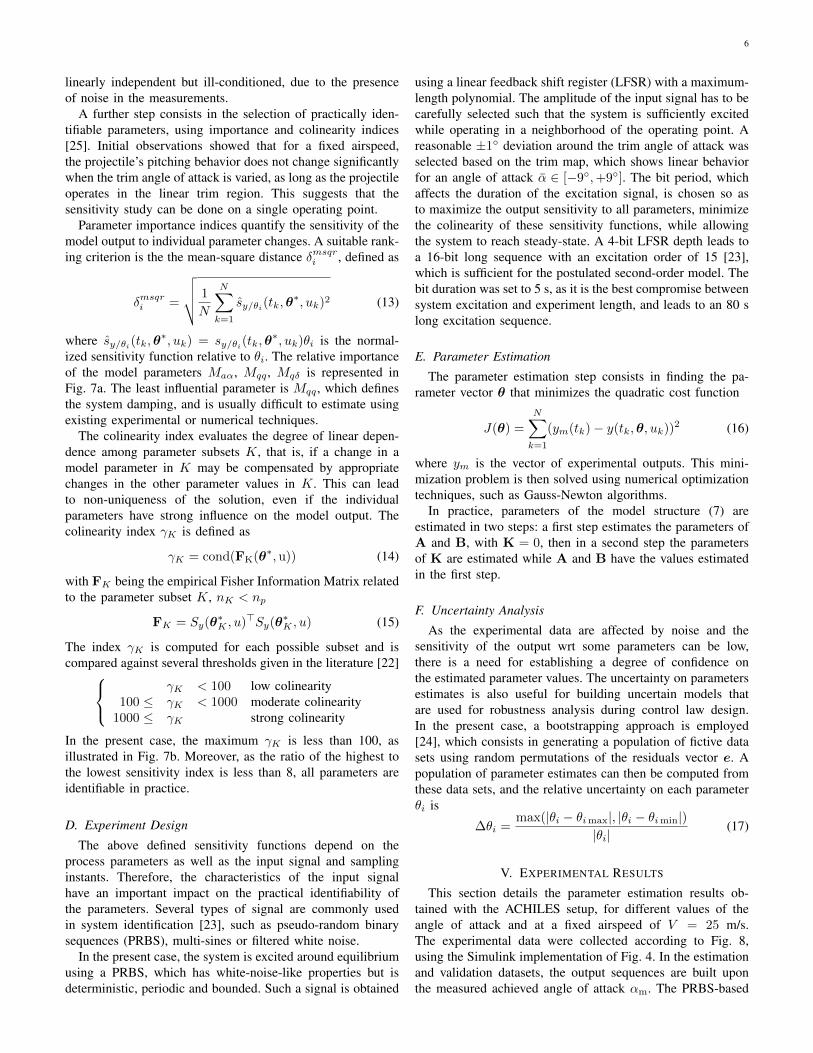
Fig. 7. Assessment of parameter identifiability using (a) the parameterimportance index δmsqri (b) the γK colinearity index of model parametersubsets, where nK denotes the size of the subset

if for almost any admissible parameter vector θ∗:

∃u ∈ RR+

, y(t,θ, u(t)) = y(t,θ∗, u(t)) ∀t ∈ R+ ⇒ θi = θ∗i(8)

A similar definition exists for local identifiability, where aneighborhood of θ∗ is considered. In the present case, theglobal a priori identifiability of the model structure (7) isassessed using a Laplace transform approach.

C. A posteriori Identifiability

A posteriori identifiability differs from a priori identifiabil-ity in that the input signal and measurement times are imposed.Even if a parameter is a priori identifiable, it may not beidentifiable in practice because of a lack of information in theexperimental data. For a given model structure, input signalu and measurement times tk, the parameter θi is a posterioriidentifiable if for almost any admissible parameter vector θ∗:

y(tk,θ, uk) = y(tk,θ∗, uk) ∀k ∈ [[1, N ]]⇒ θi = θ∗i (9)

where N is the number of samples.As with a priori identifiability, there is a local definition

where a neighborhood of θ∗ is considered. This condition canbe expressed as [22]:

∀k ∈ [[1, N ]],

np∑i=1

∂y(tk,θ, uk)

∂θi

∣∣∣∣θ∗︸ ︷︷ ︸

sy/θi (tk,θ∗,u)

·dθi = 0⇒ dθ = 0 (10)

where np is the number of parameters. In the above equation,sy/θi(tk,θ

∗, uk) is the sensitivity of the output with respectto the parameter θi, for an input signal u and measurementtime tk. This condition can also be written as:

Sy(θ∗, u) · dθ = 0⇒ dθ = 0 (11)

where Sy(θ∗, u) is the sensitivity matrix, defined as:

Sy(θ∗, u) =

sy/θ1(t1,θ∗, uk) · · · sy/θnp (t1,θ

∗, uk)...

. . ....

sy/θ1(tN ,θ∗, uk) · · · sy/θnp (tN ,θ

∗, uk)

(12)

The parameters are then locally a posteriori identifiable iffthe columns of Sy(θ∗, u) are linearly independent. In ourapplication, the sensitivity functions were derived from theoutput equation of the considered model (7), leaving out theerror model as it is estimated separately. In practice, the abovecondition is not sufficient as the sensitivity matrix may be

6

linearly independent but ill-conditioned, due to the presenceof noise in the measurements.

A further step consists in the selection of practically iden-tifiable parameters, using importance and colinearity indices[25]. Initial observations showed that for a fixed airspeed,the projectile’s pitching behavior does not change significantlywhen the trim angle of attack is varied, as long as the projectileoperates in the linear trim region. This suggests that thesensitivity study can be done on a single operating point.

Parameter importance indices quantify the sensitivity of themodel output to individual parameter changes. A suitable rank-ing criterion is the the mean-square distance δmsqri , defined as

δmsqri =

√√√√ 1

N

N∑k=1

sy/θi(tk,θ∗, uk)2 (13)

where sy/θi(tk,θ∗, uk) = sy/θi(tk,θ

∗, uk)θi is the normal-ized sensitivity function relative to θi. The relative importanceof the model parameters Maα, Mqq, Mqδ is represented inFig. 7a. The least influential parameter is Mqq, which definesthe system damping, and is usually difficult to estimate usingexisting experimental or numerical techniques.

The colinearity index evaluates the degree of linear depen-dence among parameter subsets K, that is, if a change in amodel parameter in K may be compensated by appropriatechanges in the other parameter values in K. This can leadto non-uniqueness of the solution, even if the individualparameters have strong influence on the model output. Thecolinearity index γK is defined as

γK = cond(FK(θ∗,u)) (14)

with FK being the empirical Fisher Information Matrix relatedto the parameter subset K, nK < np

FK = Sy(θ∗K , u)>Sy(θ∗K , u) (15)

The index γK is computed for each possible subset and iscompared against several thresholds given in the literature [22] γK < 100 low colinearity

100 ≤ γK < 1000 moderate colinearity1000 ≤ γK strong colinearity

In the present case, the maximum γK is less than 100, asillustrated in Fig. 7b. Moreover, as the ratio of the highest tothe lowest sensitivity index is less than 8, all parameters areidentifiable in practice.

D. Experiment Design

The above defined sensitivity functions depend on theprocess parameters as well as the input signal and samplinginstants. Therefore, the characteristics of the input signalhave an important impact on the practical identifiability ofthe parameters. Several types of signal are commonly usedin system identification [23], such as pseudo-random binarysequences (PRBS), multi-sines or filtered white noise.

In the present case, the system is excited around equilibriumusing a PRBS, which has white-noise-like properties but isdeterministic, periodic and bounded. Such a signal is obtained

using a linear feedback shift register (LFSR) with a maximum-length polynomial. The amplitude of the input signal has to becarefully selected such that the system is sufficiently excitedwhile operating in a neighborhood of the operating point. Areasonable ±1◦ deviation around the trim angle of attack wasselected based on the trim map, which shows linear behaviorfor an angle of attack α ∈ [−9◦,+9◦]. The bit period, whichaffects the duration of the excitation signal, is chosen so asto maximize the output sensitivity to all parameters, minimizethe colinearity of these sensitivity functions, while allowingthe system to reach steady-state. A 4-bit LFSR depth leads toa 16-bit long sequence with an excitation order of 15 [23],which is sufficient for the postulated second-order model. Thebit duration was set to 5 s, as it is the best compromise betweensystem excitation and experiment length, and leads to an 80 slong excitation sequence.

E. Parameter Estimation

The parameter estimation step consists in finding the pa-rameter vector θ that minimizes the quadratic cost function

J(θ) =

N∑k=1

(ym(tk)− y(tk,θ, uk))2 (16)

where ym is the vector of experimental outputs. This mini-mization problem is then solved using numerical optimizationtechniques, such as Gauss-Newton algorithms.

In practice, parameters of the model structure (7) areestimated in two steps: a first step estimates the parameters ofA and B, with K = 0, then in a second step the parametersof K are estimated while A and B have the values estimatedin the first step.

F. Uncertainty Analysis

As the experimental data are affected by noise and thesensitivity of the output wrt some parameters can be low,there is a need for establishing a degree of confidence onthe estimated parameter values. The uncertainty on parametersestimates is also useful for building uncertain models thatare used for robustness analysis during control law design.In the present case, a bootstrapping approach is employed[24], which consists in generating a population of fictive datasets using random permutations of the residuals vector e. Apopulation of parameter estimates can then be computed fromthese data sets, and the relative uncertainty on each parameterθi is

∆θi =max(|θi − θimax|, |θi − θimin|)

|θi|(17)

V. EXPERIMENTAL RESULTS

This section details the parameter estimation results ob-tained with the ACHILES setup, for different values of theangle of attack and at a fixed airspeed of V = 25 m/s.The experimental data were collected according to Fig. 8,using the Simulink implementation of Fig. 4. In the estimationand validation datasets, the output sequences are built uponthe measured achieved angle of attack αm. The PRBS-based

7

Actuators

Airframe

Model

δm,c(t) δm(t)+

αm(t)

−

αe(t)

e(t)

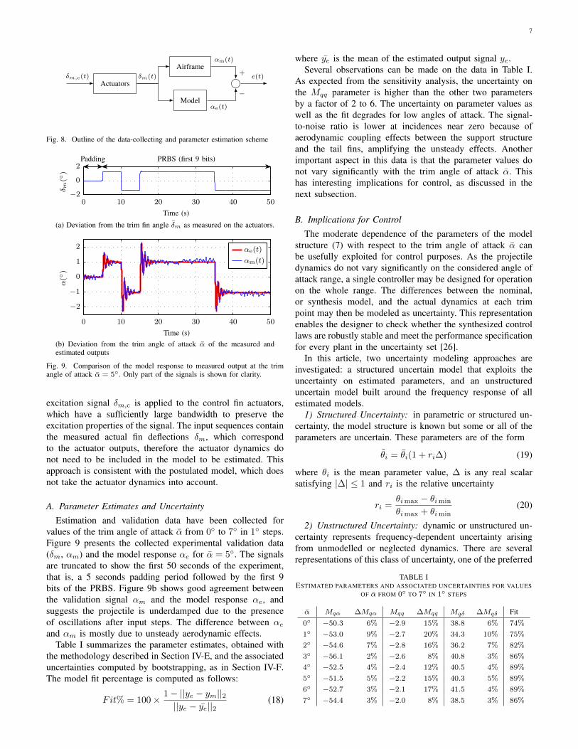
Fig. 8. Outline of the data-collecting and parameter estimation scheme

PRBS (first 9 bits)Padding

Time (s)

δm(◦)

0 10 20 30 40 50−2

0

2

(a) Deviation from the trim fin angle δm as measured on the actuators.

αm(t)

αe(t)

Time (s)

α(◦)

0 10 20 30 40 50

−2

−1

0

1

2

(b) Deviation from the trim angle of attack α of the measured andestimated outputs

Fig. 9. Comparison of the model response to measured output at the trimangle of attack α = 5◦. Only part of the signals is shown for clarity.

excitation signal δm,c is applied to the control fin actuators,which have a sufficiently large bandwidth to preserve theexcitation properties of the signal. The input sequences containthe measured actual fin deflections δm, which correspondto the actuator outputs, therefore the actuator dynamics donot need to be included in the model to be estimated. Thisapproach is consistent with the postulated model, which doesnot take the actuator dynamics into account.

A. Parameter Estimates and Uncertainty

Estimation and validation data have been collected forvalues of the trim angle of attack α from 0◦ to 7◦ in 1◦ steps.Figure 9 presents the collected experimental validation data(δm, αm) and the model response αe for α = 5◦. The signalsare truncated to show the first 50 seconds of the experiment,that is, a 5 seconds padding period followed by the first 9bits of the PRBS. Figure 9b shows good agreement betweenthe validation signal αm and the model response αe, andsuggests the projectile is underdamped due to the presenceof oscillations after input steps. The difference between αeand αm is mostly due to unsteady aerodynamic effects.

Table I summarizes the parameter estimates, obtained withthe methodology described in Section IV-E, and the associateduncertainties computed by bootstrapping, as in Section IV-F.The model fit percentage is computed as follows:

Fit% = 100× 1− ||ye − ym||2||ye − ye||2

(18)

where ye is the mean of the estimated output signal ye.Several observations can be made on the data in Table I.

As expected from the sensitivity analysis, the uncertainty onthe Mqq parameter is higher than the other two parametersby a factor of 2 to 6. The uncertainty on parameter values aswell as the fit degrades for low angles of attack. The signal-to-noise ratio is lower at incidences near zero because ofaerodynamic coupling effects between the support structureand the tail fins, amplifying the unsteady effects. Anotherimportant aspect in this data is that the parameter values donot vary significantly with the trim angle of attack α. Thishas interesting implications for control, as discussed in thenext subsection.

B. Implications for Control

The moderate dependence of the parameters of the modelstructure (7) with respect to the trim angle of attack α canbe usefully exploited for control purposes. As the projectiledynamics do not vary significantly on the considered angle ofattack range, a single controller may be designed for operationon the whole range. The differences between the nominal,or synthesis model, and the actual dynamics at each trimpoint may then be modeled as uncertainty. This representationenables the designer to check whether the synthesized controllaws are robustly stable and meet the performance specificationfor every plant in the uncertainty set [26].

In this article, two uncertainty modeling approaches areinvestigated: a structured uncertain model that exploits theuncertainty on estimated parameters, and an unstructureduncertain model built around the frequency response of allestimated models.

1) Structured Uncertainty: in parametric or structured un-certainty, the model structure is known but some or all of theparameters are uncertain. These parameters are of the form

θi = θi(1 + ri∆) (19)

where θi is the mean parameter value, ∆ is any real scalarsatisfying |∆| ≤ 1 and ri is the relative uncertainty

ri =θimax − θimin

θimax + θimin(20)

2) Unstructured Uncertainty: dynamic or unstructured un-certainty represents frequency-dependent uncertainty arisingfrom unmodelled or neglected dynamics. There are severalrepresentations of this class of uncertainty, one of the preferred

TABLE IESTIMATED PARAMETERS AND ASSOCIATED UNCERTAINTIES FOR VALUES

OF α FROM 0◦ TO 7◦ IN 1◦ STEPS

α Mqα ∆Mqα Mqq ∆Mqq Mqδ ∆Mqδ Fit

0◦ −50.3 6% −2.9 15% 38.8 6% 74%

1◦ −53.0 9% −2.7 20% 34.3 10% 75%

2◦ −54.6 7% −2.8 16% 36.2 7% 82%

3◦ −56.1 2% −2.6 8% 40.8 3% 86%

4◦ −52.5 4% −2.4 12% 40.5 4% 89%

5◦ −51.5 5% −2.2 15% 40.3 5% 89%

6◦ −52.7 3% −2.1 17% 41.5 4% 89%

7◦ −54.4 3% −2.0 8% 38.5 3% 86%

8

∣

∣

∣

Gp(jω)−G(jω)

G(jω)

∣

∣

∣

|wI |

Mag

nit

ud

e(d

B)

Frequency (rad/s)

10−1

100

101

102

−20

−15

−10

−5

Fig. 10. Relative errors in the unstructured uncertainty case. Solid line:second-order weight |wI | in (21)

Unstructured uncertainty

Parametric uncertainty

Estimated models

Mag

nit

ud

e(d

B)

Frequency (rad/s)

10−1

100

101

102

−60

−40

−20

0

20

Fig. 11. Envelope of estimated and bootstrapped responses against parametricand unstructured uncertainty envelopes

form being multiplicative uncertainty [26], where the set ofpossible perturbed models ΠI contains models of the form

Gp(s) = G(s)(1 + wI(s)∆I(s)) (21)

where G(s) is the nominal plant model, ∆I is any stabletransfer function satisfying |∆I(jω)| ≤ 1, ∀ω and the mul-tiplicative weight wI is a stable and minimum-phase transferfunction, satisfying |wI(jω)| ≥ lI(ω), ∀ω. The uncertaintyradius lI(ω) is defined as:

lI(ω) = maxGp∈Π

∣∣∣∣Gp(jω)−G(jω)

G(jω)

∣∣∣∣ , ∀ω (22)

In the present case, the parameters of the nominal model Gare the mean values of the complete set of parameters and Πcontains all estimated models. The relative error |Gp−G|/|G|and the bounding multiplicative weight wI , which here is asecond-order filter, are presented in Fig. 10. The uncertaintysize is 13.6% and 20.8% at respectively low and high fre-quencies, and the maximum uncertainty attains 38.5% at theresonance peak, situated in middle frequencies.

The uncertainty envelopes for the two considered model-ing approaches are compared to the envelope of estimatedmodels in Fig. 11. The parametric uncertain model is moreconservative than the unstructured description with a relativeuncertainty of 21.9% at low frequencies, and has a similarbehavior at medium to high frequencies. For control purposes,the system has a relatively consistent behavior across theconsidered flight envelope, with a moderately varying dampingratio. Although the uncertainty is not negligible, it can beproperly handled with robust control techniques such as H∞control [26].

VI. CONCLUSION

In this paper, the focus was put on the identification of thepitch axis dynamics of the ACHILES setup. The projectile’sbehavior is expressed as a nonlinear model governed by thelaws of flight dynamics. A linearized q-LPV model is obtainedaround the projectile equilibrium point, and considered forestimation around a fixed operating point with the additionof a noise model. A priori and a posteriori identifiabilitystudies were conducted and show that the parameters of theproposed model are identifiable. The model parameters havebeen estimated for different values of the trim angle of attackat a constant airspeed V = 25 m/s. The results show goodagreement with the validation data and moderate dependencewith respect to the trim angle of attack. Uncertain models ofthe projectile’s dynamic behavior have then been built usingthe estimation results.

As future work, the approaches described herein will beapplied to the projectile pitch and yaw axes in coupled motion,and associated control laws will be developed. A secondresearch axis will focus on the airspeed dependence of thedeveloped models and the associated control issues.

REFERENCES

[1] F. Fresconi, “Guidance and control of a projectile with reduced sensorand actuator requirements,” Journal of Guidance, Control, and Dynam-ics, vol. 34, no. 6, pp. 1757–1766, 2011.

[2] M. Costello, “Extended range of a gun launched smart projectile usingcontrollable canards,” Shock and Vibration, vol. 8, no. 3, pp. 203–213,Jan. 2001.

[3] S. Theodoulis, V. Gassmann, P. Wernert, L. Dritsas, I. Kitsios, andA. Tzes, “Guidance and control design for a class of spin-stabilizedfin-controlled projectiles,” Journal of Guidance, Control, and Dynamics,vol. 36, no. 2, 2013.

[4] A. J. Calise, M. Sharma, and J. E. Corban, “Adaptive autopilot designfor guided munitions,” Journal of Guidance, Control, and Dynamics,vol. 23, no. 5, pp. 837–843, Sep. 2000.

[5] P. H. Zipfel, Modeling and Simulation of Aerospace Vehicle Dynamics.American Institute of Aeronautics and Astronautics, 2007.

[6] P. Weinacht, “Projectile performance, stability, and free-flight motionprediction using computational fluid dynamics,” Journal of Spacecraftand Rockets, vol. 41, no. 2, pp. 257–263, 2004.

[7] R. Whyte, “PRODAS - projectile analysis,” Arrow Tech Associates,South Burlington, VT, Tech. Rep., 1991.

[8] W. B. Blake, “Missile DATCOM: User’s manual - 1997 FORTRAN 90revision,” DTIC Document, Tech. Rep., 1998.

[9] J. B. Barlow, W. H. Rae, and A. Pope, Low-Speed Wind Tunnel Testing,Third Edition. Wiley New York, 1999.

[10] M. Albisser, S. Dobre, C. Berner, M. Thomassin, and H. Garnier,“Identifiability investigation of the aerodynamic coefficients from freeflight tests,” in AIAA Atmospheric Flight Mechanics Conference, 2013.

[11] M. Bacic, “On hardware-in-the-loop simulation,” in IEEE Conferenceon Decision and Control and European Control Conference, 2005, pp.3194–3198.

[12] R. Verma, D. D. Vecchio, and H. K. Fathy, “Development of a scaledvehicle with longitudinal dynamics of an hmmwv for an its testbed,”IEEE/ASME Transactions on Mechatronics, vol. 13, no. 1, pp. 46–57,Feb. 2008.

[13] F. Fresconi, I. Celmins, M. Ilg, and J. Maley, “Projectile roll dynamicsand control with a low-cost maneuver system,” Journal of Spacecraftand Rockets, vol. 51, no. 2, pp. 624–627, Mar. 2014.

[14] J. Ma, H. Kharboutly, A. Benali, F. B. Amar, and M. Bouzit, “Designof omnidirectional mobile platform for balance analysis,” IEEE/ASMETransactions on Mechatronics, vol. 19, no. 6, pp. 1872–1881, Dec. 2014.

[15] J. Laut, E. Henry, O. Nov, and M. Porfiri, “Development of amechatronics-based citizen science platform for aquatic environmentalmonitoring,” IEEE/ASME Transactions on Mechatronics, vol. 19, no. 5,pp. 1541–1551, Oct. 2014.

9

[16] S. Omari, M.-D. Hua, G. Ducard, and T. Hamel, “Hardware and softwarearchitecture for nonlinear control of multirotor helicopters,” IEEE/ASMETransactions on Mechatronics, vol. 18, no. 6, pp. 1724–1736, Dec. 2013.

[17] P. Apkarian and D. Noll, “Nonsmooth H∞ synthesis,” IEEE Transac-tions on Automatic Control, vol. 51, no. 1, pp. 71—86, 2006.

[18] P. Gerum, “Xenomai - implementing a rtos emulation frameworkon gnu/linux,” White Paper: http://www.xenomai.org, 2004. [Online].Available: http://www.xenomai.org/documentation/branches/v2.3.x/pdf/xenomai.pdf

[19] D. Leith and W. Leithead, “Survey of gain-scheduling analysis anddesign,” International Journal of Control, vol. 73, no. 11, p. 1001–1025,2000.

[20] F. R. Garza and E. A. Morelli, “A collection of nonlinear aircraft sim-ulations in matlab,” NASA Langley Research Center, Technical ReportNASA/TM, vol. 212145, 2003.

[21] J. Hadamard, “Sur les problemes aux derivees partielles et leur significa-tion physique,” Princeton University Bulletin, vol. 13, no. 49-52, p. 28,1902.

[22] S. Dobre, “Global sensitivity and identifiability analyses. application toestimation of photophysical parameters in photodynamic therapy,” Ph.D.dissertation, Universite Henri Poincare-Nancy I, 2010.

[23] L. Ljung, System Identification - Theory for the User. Prentice-Hall,1999.

[24] E. Walter and L. Pronzato, Identification of Parametric Models fromExperimental Data. Springer, 1997.

[25] R. Brun, P. Reichert, and H. R. Kunsch, “Practical identifiability analysisof large environmental simulation models,” Water Resources Research,vol. 37, no. 4, p. 1015–1030, 2001.

[26] S. Skogestad and I. Postlethwaite, Multivariable Feedback Control:Analysis and Design, Second Edition. Wiley New York, 2007, vol. 2.