PIGI 4.3

Construction manual and operation instructions

This document is a supplement to:

Izett, R. W., and Tortell., P. D. 2020. The Pressure of In-situ Gases Instrument (PIGI) for

autonomous ship-board measurement of dissolved O2 and N2 in surface ocean waters.

Oceanography. Accepted.

Updated: July 2020

Robert Izett

University of British Columbia

rizett@eoas.ubc.ca

This document contains a list of recommended parts and suppliers (section S1), instructions for

assembling the PIGI system (section S2), instructions for operation (section S3), and a

description of additional files (e.g. technical drawings) and author-provided software (section

S4), including the acquisition and processing software. Additional details on the workflow of the

acquisition and processing software are provided to facilitate the development of software

packages on other platforms (section S5).

PIGI system updates since previous version:

N/A

Document updates since previous version:

N/A

Software updates since previous version:

N/A

Additional supplementary files:

PIGI4.3_Technical-drawings.pdf: This file contains technical drawings and specifications for the

machined parts of the PIGI system (see section S2). Parts A-K correspond with the labelled parts

in Diagrams 1-6. Drawings were produced using Solidworks software. 3D CAD assembly and

parts files are also provided at github.com/rizett/PIGI_system.

PIGI_Opt-chamber-cleaning.mp4: This file contains a brief video outlining the steps to clean the

Optode chamber.

Software files: Software for running the PIGI system and processing output data are provided at

github.com/rizett/PIGI_system. LabVIEW acquisition (including an installer for the run-time

engine executable files), AutoIt restart automation and Matlab processing scripts are provided.

NOTE: The files contained in this manuscript and supplement are duplicated at

seawize.weebly.com/PIGI-system. Refer to this site for updates to the PIGI system, post-

publication.

S1. Recommended parts

Table S1. Detailed parts list and link to source (click on part name). We provide recommended

parts based on specifications required for best performance and in adherence with the system

designs provided here. However, some parts are non-specific and can be purchased from other

sources or replaced with equivalent components. The approximate cost column shows the total

cost for all components on each line of the table. Assembly notes refer to the numbered footnotes

below the tables. A. Wet box instruments

Part (with link to source) Required Approx. cost

(USD) Specs.

Assembly

note

1 Aanderaa Optode 4330 1 6,750 5-14 VDC 1

2 Pro-Oceanus TDGP-mini 1 5,000 6-24 VDC 2

3 TDGP flow-through head 1 180

4 Instrument pump 1 230 24 VDC; 1.1 gal/min

(max) 3

5 Instruments flow meter 1 9 5-12 VDC; 0.3 – 6

L/min; 7 mm barb 4

6 Primary chamber flow meter 1 10 5-18 VDC; 1-30

L/min; 1/2" MNPS 4

B. Wet box: raw materials and additional parts

Part (with link to source) Required Approx. cost

(USD) Specs.

Assembly

note

7 Pelican case iM2720 1 230 22" x 17" x 10"

(interior)

8 Debubbling tube 1 2 3” long 5

9 Bulkhead connector for

debubbler

1 17

10 PVC sheeting 1 300 various thickness 6

11 Arcylic tube (for primary

chamber)

1 65 4" ID; 4.5" OD; 5"

length 7

12 Arcylic tube (for inst. chamber) 1 65 3" ID; 3.5" OD; 4.5"

length 7

13 Optode o-ring 1 11 1.7" OD 8

14 Optode chamber o-ring (inflow) 1 10 3" OD 8

15 Optode chamber o-ring (outflow) 1 10 3" OD 8

16 Primary chamber o-ring (inflow) 1 10 4" OD 8

17 Primary chamber o-ring (outflow) 1 10 4" OD 8

18 3/8" staright valve 2 14 PVC ball valve

19 3/8" elbow valve 2 17 PVC ball valve

20 3/8" tubing 5 ft 15 silicone 9

21 Tubing insulation 1 3 5/8" ID 10

22 3/8" T-junction 1 4 3/8” FNPT 11

23 3/8" check valve 1 15 3/8” MNPT 12

24 3/8" – 1/2" adapter 1 4 3/8” FNPT x 1/2"

MNPT 13

25 1/2" check valve 1 16 1/2" MNPT 14

26 1/2" T valve 1 55 1/2” FNPT 15

27 3/8" tubing adapter 1 10 3/8" MNPT x 1/4"

barb 16

28 3/8" compression fitting 2 5 3/8" compression

tube x 3/8" barb 17

29 Flow control orifice valve 1 175 18

30 1/4"-20 wing nut 12-22 13 316-SS 19

31 1/4"-20 acorn nut 8 7 316-SS 19

32 1/4"-20 threaded rod 8 20 316-SS 19,20

33 2" 1/4"-20 screw 5-10 8 316-SS 19

34 1/4"-20 thumb screw 10-20 35 316-SS 19

35 1/4"-20 Teflon screw 2 10 1.5" long 21

36 Compression pads 4 40 22

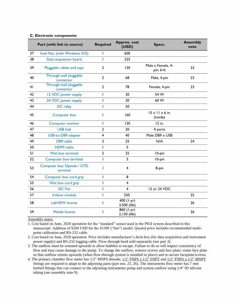
C. Electronic components

Part (with link to source) Required Approx. cost

(USD) Specs.

Assembly

note

37 Intel Nuc (with Windows O/S) 1 600

38 Data acquisition board 1 225

39 Pluggable cables and caps 2 130 Male x Female, 4-

pin; 6-ft 23

40 Through-wall pluggable

connector

2 68 Male, 4-pin 23

41 Through-wall pluggable

connector

2 78 Female, 4-pin 23

42 12 VDC power supply 1 20 54 W

43 24 VDC power supply 1 20 60 W

44 DC relay 1 50

45 Computer box 1 160 15 x 11 x 6 in.

(inside)

46 Computer monitor 1 130 12 in.

47 USB hub 2 20 4 ports

48 USB-to-DB9 adapter 4 40 Male DB9 x USB

49 DB9 cable 3 25 N/A 24

50 HDMI cable 1 5

51 Wet box terminal 2 25 10-pin

52 Computer box terminal 1 5 10-pin

53 Computer box Optode / GTD

terminal

1 4 8-pin

54 Computer box cord grip 1 8

55 Wet box cord grip 1 4

56 DC Fan 1 4 12 or 24 VDC

57 Iridium module 1 250 25

58 LabVIEW license 1 400 (1-yr)

3,500 (life) 26

59 Matlab license 1 860 (1-yr)

2,150 (life) 26

Assembly notes:

1. Cost based on June, 2020 quotation for the “standard” sensor used in the PIGI system described in this

manuscript. Addition of $200 USD for the 4330F (“fast”) model. Quoted price includes recommended multi-

point calibration and RS-232 cable.

2. Cost based on June, 2020 quotation. Price includes manufacturer’s deck-box (for data acquisition and instrument

power supply) and RS-232 logging cable. Flow-through head sold separately (see part 3).

3. The outflow must be oriented upwards to allow bubbles to escape. Failure to do so will impact consistency of

flow and may cause damage to the pump. To change the outflow, remove screws and face plate; rotate face plate

so that outflow orients upwards (when flow-through system is installed in place) and re-secure faceplate/screws.

4. The primary chamber flow meter has 1/2" MNPS threads; 1/2" FNPS x 1/2" FNPT and 1/2" FNPS x 1/2" MNPT

fittings are required to adapt to the adjoining parts (part nos. 25, 26). The instruments flow meter has 7 mm

barbed fittings that can connect to the adjoining instruments pump and system outflow using 1/4" ID silicone

tubing (see assembly note 9).

5. The “debubbler” is simply a porous PVC tube, which allows bubbles to escape from the primary chamber and

filters out coarse particulates. To fabricate it, drill small (~1/8” – 1/4”) holes through the tube, and cover with a

coarse plastic mesh. Secure the mesh with rubber bands or zip-ties.

6. Requires 0.5", 1", 1.5" and 2" thick sheeting to construct flow-through parts.

7. Recommended minimum wall thickness of 0.25".

8. Recommended to replace often.

9. 3/8" tubing between interior components of flow through system. Small sections of 1/4" tubing will be required to

connect between the outflow of the instruments pump and inflow of the instruments flow meter, and between the

outflow the instruments flow meter and system outflow. Tubing to system and seawater supply will vary.

10. Tubing insulation prevents condensation inside wet box.

11. Intersection between (a) outflow of the instrument flow meter, (b) outflow to the discrete sampling line, and (c)

rejoin with outflow of primary chamber.

12. Recommended to prevent back-flow through the instrument chamber.

13. Required to adapt between instrument loop and primary chamber.

14. Recommended to prevent back-flow through the primary chamber.

15. Intersection between (a) outflow of the primary chamber, (b) outflow from instrument loop, and (c) system

outflow.

16. This part, and others, may be required to connect the outflows from the primary and instrument chambers.

17. Required to adapt to instrument flow meter.

18. This part should be installed between the outflow of the primary chamber and the instrument loop to dampen

flow-rate surges in the main seawater supply that produce hydrostatic pressure responses in the GTD readings.

19. 316-SS recommended for best corrosion resistance.

20. Cut to 7" (x2), 8" (x4), 9" (x2).

21. To secure GTD.

22. Optional: install on the under-side of the base plate and/or Pelican case for shock-resistance. Use thicker pads if

desired.

23. Use pluggable connectors to easily (dis)connect the Optode and GTD between the wet and computer boxes. One

set required each for Optode and GTD. Caps (for cable and through-wall connectors) and locking nuts are also

required.

24. Cut two short cables (6 ft) for wiring connections inside the computer and wet boxes. Use a long cable (>6 ft) to

connect between the computer and wet box.

25. Optional. A second computer, with a view to the sky, may be required.

26. Optional. A LabVIEW license (for the 2019 SP1 development program) is required to modify the LabVIEW

software scripts provided here. However, the LabVIEW run-time engine is available, free-of-charge, and can be

used to run our software. If using the stand-alone executable, run the provided installer to install the necessary

files, programs and drivers. Run the acquisition as described below in section 4. A Matlab license is required to

run the Matlab processing scripts, but section S5 provides details for developing scripts using non-proprietary

programs.

S2. Assembly instructions

The instructions below provide step-by-step details on the assembly of the wet and electronics

boxes of the PIGI system. Numbered parts refer to those listed in Table S1.

NOTE: These instructions are provided as-is. Please read through them carefully before

proceeding. Exercise care when working with electrical components and consult the

instrument manufacturers if you have reservations about cutting cables. The authors are

not liable for personal or instrument harm.

S2.1 Flow-through system (wet box)

1. Machine the components of the flow-through system (Parts A-K) from the raw PVC

sheeting (part no. 10; Table S1) and acrylic tubes (part nos. 11, 12) following the

specifications in (refer to PIGI4.3_Technical-drawings.pdf in the additional

supplementary files).

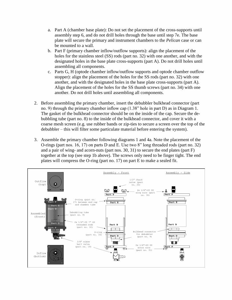
a. Part A (chamber base plate): Do not set the placement of the cross-supports until

assembly step 6, and do not drill holes through the base until step 7e. The base

plate will secure the primary and instrument chambers to the Pelican case or can

be mounted to a wall.

b. Part F (primary chamber inflow/outflow supports): align the placement of the

holes for the stainless steel (SS) rods (part no. 32) with one another, and with the

designated holes in the base plate cross-supports (part A). Do not drill holes until

assembling all components.

c. Parts G, H (optode chamber inflow/outflow supports and optode chamber outflow

stopper): align the placement of the holes for the SS rods (part no. 32) with one

another, and with the designated holes in the base plate cross-supports (part A).

Align the placement of the holes for the SS thumb screws (part no. 34) with one

another. Do not drill holes until assembling all components.

2. Before assembling the primary chamber, insert the debubbler bulkhead connector (part

no. 9) through the primary chamber inflow cap (1.38” hole in part D) as in Diagram 1.

The gasket of the bulkhead connector should be on the inside of the cap. Secure the de-

bubbling tube (part no. 8) to the inside of the bulkhead connector, and cover it with a

coarse mesh screen (e.g. use rubber bands or zip-ties to secure a screen over the top of the

debubbler – this will filter some particulate material before entering the system).

3. Assemble the primary chamber following diagrams 1 and 4a. Note the placement of the

O-rings (part nos. 16, 17) on parts D and E. Use two 8” long threaded rods (part no. 32)

and a pair of wing- and acorn-nuts (part nos. 30, 31) to secure the end plates (part F)

together at the top (see step 1b above). The screws only need to be finger tight. The end

plates will compress the O-ring (part no. 17) on part E to make a sealed fit.

3/8” elbow

ball valve

(part no. 19)

O-ring (part no.

17) between end cap

and chamber tube

O-ring

(part no. 16)

(a) (b)

2x 1/4”-20 SS

acorn nuts

(part no. 31)

2x 1/4”-20 7” SS

threaded rods

(part no. 32)

2x 1/4”-20 SS

wing nuts (part

no. 30)

Part B

Part F

Part F

Part D

Part E

1/2” Check

valve (part

no. 25)

Bulkhead connector

for debubbler

(part no. 9)

Outflow

(top)

Inflow

(bottom)

Debubbling tube

(part no. 8)

Assembly - Front Assembly - Side

Assembled

(front)

Part B

Part F

Part F

Part D

Part E

Part B

Part F

Part F

Part D

Part E

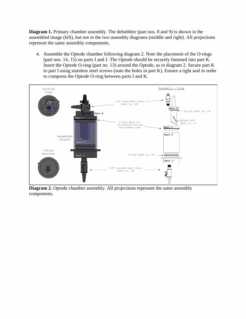
Diagram 1. Primary chamber assembly. The debubbler (part nos. 8 and 9) is shown in the

assembled image (left), but not in the two assembly diagrams (middle and right). All projections

represent the same assembly components.

4. Assemble the Optode chamber following diagram 2. Note the placement of the O-rings

(part nos. 14, 15) on parts I and J. The Optode should be securely fastened into part K.

Insert the Optode O-ring (part no. 13) around the Optode, as in diagram 2. Secure part K

to part I using stainless steel screws (note the holes in part K). Ensure a tight seal in order

to compress the Optode O-ring between parts I and K.

Diagram 2. Optode chamber assembly. All projections represent the same assembly

components.

Optode 4330

(part no. 1)

3/8” straight ball valve

(part no. 18)

3/8” elbow ball valve

(part no. 19)

O-ring (part no.

15) between end cap

and chamber tube

O-ring (part no. 14)

K

O-ring (part no. 13)

Assembly - Side

Part K

Part I

Part C

Part J

Outflow

(top)

Inflow

(bottom)

Assembled

(front)

Part K

Part I

Part C

Part J

5. Assemble the rest of the instrument chamber following diagrams 3 and 4b. Secure the

GTD through the holes in parts G and H using Teflon screws (part no. 35). Use two 7”

long threaded rods (part no. 32) and a pair of wing- and acorn-nuts (nos. 30, 31) to secure

the end plates (part G) and optode chamber support (part H) together at the top, and use

four thumb screws (part no. 34) and wing-nuts to fasten parts G and H together (see step

1c above) The screws only need to be finger tight. The end plates will compress the O-

ring on part I of the Optode chamber to make a sealed fit with the chamber tube (part C).

Diagram 3. Instrument chamber assembly. All projections represent the same assembly

components.

2x 1/4”-20 SS acorn

nuts (part no. 31)

2x 1/4”-20 8” SS threaded

rods (part no. 32)

4x 1/4”-20 SS wing

nuts (part no. 30)

4x 1/4”-20 SS thumb screws (part no.

34)

Teflon screw

Mini-

TDGP

(part

no.

2)

Optode

chamber

Teflon screws

(part no. 35)G

Outflow

(top)

Inflow

(bottom)

Assembly - Front

Assembled

(front)

Part H

Part G

Part G

Part H

Part G

Part G

Diagram 4. Assembled primary (a) and instrument (b) chambers. The debubbling components

(part nos. 8, 9) are not shown in (a). Labelled parts correspond with the machined components in

PIGI4.3_Technical-drawings.pdf.

6. Following diagrams 5b and 6, install the plumbing components at the outflow of the

primary chamber:

a. Install the 1/2” check valve (part no. 25) at the outflow of the primary chamber

(see 1/2” NPT hole labelled on part E in PIGI4.3_Technical-drawings.pdf in the

additional supplementary files). Note the direction of the valve to prevent back-

flow into the primary chamber.

b. Connect the primary chamber flow meter (part no. 6) to the check valve at the

outflow of the primary chamber.

c. Assemble the pipe fittings at the outflow of the primary chamber flow meter.

Connect the 3-way valve (part no. 26) directly to the flow meter. One of the

remaining ports on the valve will direct water to the system outflow, and the

remaining port will connect to the instrument loop. Connect the 1/2”-3/8” adapter

(part no. 24), 3/8” T-junction (part no. 22) and 3/8” check valve (part no. 23) as in

diagrams 5b and 6. Note the direction of the check valve and seawater flow (see

arrows in diagram 6) to prevent back-flow into the instrument loop.

i. Use the 3-way manual valve (part no. 26) to isolate different components

of the system. For example, the valve can be closed to prevent circulation

through either the primary or instrument chambers. The fittings to connect

the valve to the system outflow will vary by deployment / ship. Flexible

Tygon tubing is recommended where possible.

7. Once the primary and instrument chambers are assembled, decide on the placement of the

base plate (part A) cross-supports. Secure the supports to the base plate using stainless

steel screws or glue. Following diagram 5, secure the primary and instrument chambers

between the cross-supports.

(a) (b)

E

Outflow

(top)

Inflow

(bottom)

Assembled

(side)

Outflow

(top)

Inflow

(bottom)

Assembled

(side)

D

F

F

F

E

F

DB

G

J

G

K

C

K

J

H

G

G

I

HTDGP-mini

Optode

a. Use two 9” long threaded rods (part no. 32) and a pair of wing- and acorn-nuts

(part nos. 30, 31) to secure the primary chamber to the base plate (see step 1b

above). The screws only need to be finger tight.

b. Use two 8” long threaded rods (part no. 32) and a pair of wing- and acorn-nuts

(part nos. 30, 31) to secure the instrument chamber to the base plate (see step 1c

above). The screws only need to be finger tight.

NOTE: The faces of the Optode and GTD should face downwards, with the flow of water

directed onto them.

Diagram 5. Assembled flow-through chambers on based plate (Pelican case shown in green in

panel (b)). Panel (b) shows the top-down view, and panel (c) shows the side and front views.

Numbered parts in panel (b) represent the plumbing components at the outflow of the primary

chamber and correspond with labelled parts in Diagram 6, and Table S1.

8. Following diagram 6, assemble the remaining ancillary components of the wet box.

a. Install the instrument pump (part no. 4) and instrument flow meter (part no. 5)

downstream of the instrument chamber by securing them to the Pelican case or

base plate. Insert the compression / barb fittings (part no. 28) into the inflow and

outflow ports of the flow meter.

b. Connect the primary and instrument chambers using the 3/8” tubing (blue lines in

diagram 6; part no. 20) and connect the outflow of the Optode chamber to the

pump and flow meter. Connect the outflow from the instrument flow meter to the

outflow of the primary chamber and install the fittings (part nos. 18, 22, 23, 27)

for the discrete sampling line. Note that 1/4" tubing is required to connect the

instruments flow meter to the adjacent parts (see assembly note for part no. 20).

Use worm-drive clamps / hose clamps as necessary to secure the tubing to the

barbed GTD flow-through head, valves and fittings.

(a) (b) (c)

To secure to base of Pelican Case

with SS screws (part no. 33)

Compression pads (part no. 36)

Part A

Up

24

6

22 26

27

25

18

Primary

Chamber

Instrument

Chamber

Pelican case (part no. 7)

23 To out

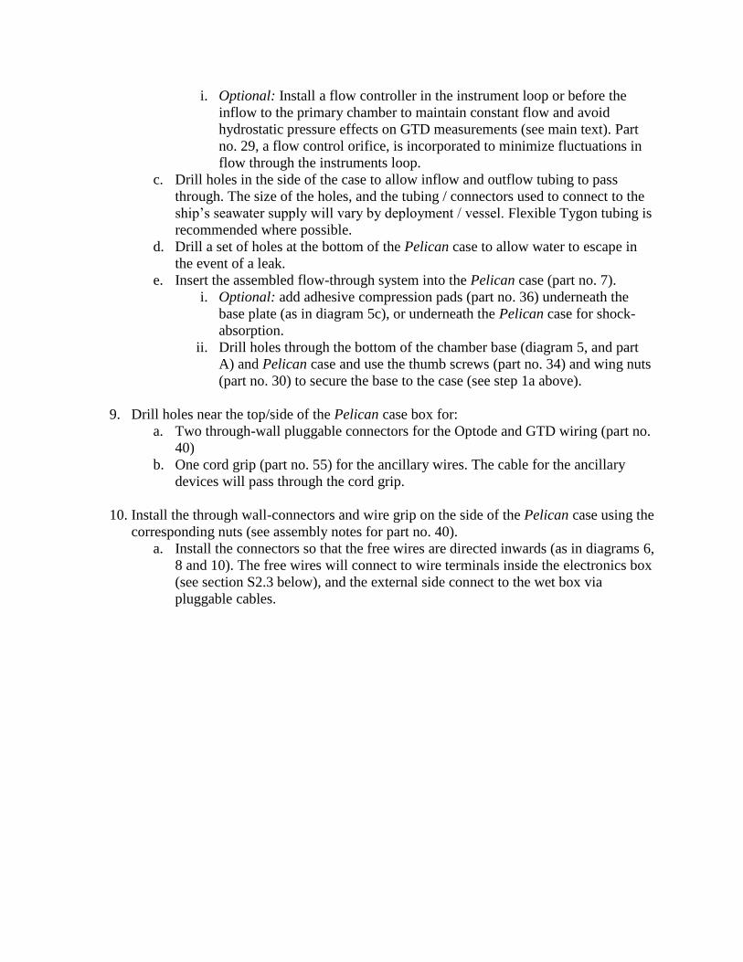
i. Optional: Install a flow controller in the instrument loop or before the

inflow to the primary chamber to maintain constant flow and avoid

hydrostatic pressure effects on GTD measurements (see main text). Part

no. 29, a flow control orifice, is incorporated to minimize fluctuations in

flow through the instruments loop.

c. Drill holes in the side of the case to allow inflow and outflow tubing to pass

through. The size of the holes, and the tubing / connectors used to connect to the

ship’s seawater supply will vary by deployment / vessel. Flexible Tygon tubing is

recommended where possible.

d. Drill a set of holes at the bottom of the Pelican case to allow water to escape in

the event of a leak.

e. Insert the assembled flow-through system into the Pelican case (part no. 7).

i. Optional: add adhesive compression pads (part no. 36) underneath the

base plate (as in diagram 5c), or underneath the Pelican case for shock-

absorption.

ii. Drill holes through the bottom of the chamber base (diagram 5, and part

A) and Pelican case and use the thumb screws (part no. 34) and wing nuts

(part no. 30) to secure the base to the case (see step 1a above).

9. Drill holes near the top/side of the Pelican case box for:

a. Two through-wall pluggable connectors for the Optode and GTD wiring (part no.

40)

b. One cord grip (part no. 55) for the ancillary wires. The cable for the ancillary

devices will pass through the cord grip.

10. Install the through wall-connectors and wire grip on the side of the Pelican case using the

corresponding nuts (see assembly notes for part no. 40).

a. Install the connectors so that the free wires are directed inwards (as in diagrams 6,

8 and 10). The free wires will connect to wire terminals inside the electronics box

(see section S2.3 below), and the external side connect to the wet box via

pluggable cables.

Diagram 6. A schematic of the wet box assembly showing the top-down view of the base of the

Pelican case (left) and an inside side panel (right).

= valve

= T-junction

= check (one-

way) valve

= 3/8” tubing

= wiring

terminals

#

(51) Enclosed wire terminal

(24)

Primary

chamber Optode

chamber

(7) Pelican case

In

Out

Flow meter

(4)

Pump

(1) Optode

(8) De-

bubbler

(2)

GTD

Sampling

line

up

(3)

(5)

(9)

(18)

(18)

(19)

(19)

(20/21)

(22) (26)

(27)

(23)

(25)

bottom side

1 2 3 4 5 6 7 8

1 2 3 4 5 6 7 8

(40) Through-wall

pluggable

connectors

(55) Cord grip

(6)

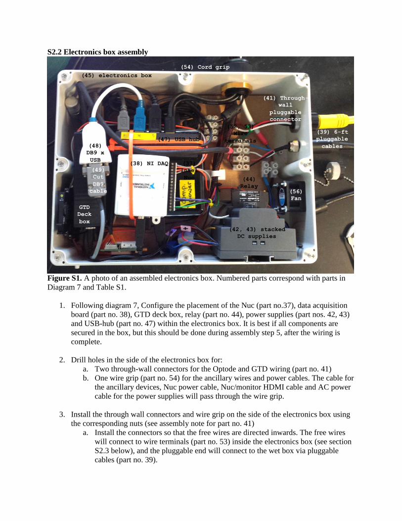
S2.2 Electronics box assembly

Figure S1. A photo of an assembled electronics box. Numbered parts correspond with parts in

Diagram 7 and Table S1.

1. Following diagram 7, Configure the placement of the Nuc (part no.37), data acquisition

board (part no. 38), GTD deck box, relay (part no. 44), power supplies (part nos. 42, 43)

and USB-hub (part no. 47) within the electronics box. It is best if all components are

secured in the box, but this should be done during assembly step 5, after the wiring is

complete.

2. Drill holes in the side of the electronics box for:

a. Two through-wall connectors for the Optode and GTD wiring (part no. 41)

b. One wire grip (part no. 54) for the ancillary wires and power cables. The cable for

the ancillary devices, Nuc power cable, Nuc/monitor HDMI cable and AC power

cable for the power supplies will pass through the wire grip.

3. Install the through wall connectors and wire grip on the side of the electronics box using

the corresponding nuts (see assembly note for part no. 41)

a. Install the connectors so that the free wires are directed inwards. The free wires

will connect to wire terminals (part no. 53) inside the electronics box (see section

S2.3 below), and the pluggable end will connect to the wet box via pluggable

cables (part no. 39).

GTD

Deck

box

(37)

Intel

Nuc

(38) NI DAQ

(45) electronics box

(42, 43) stacked

DC supplies

(47) USB hub

(41) Through-

wall

pluggable

connector

(54) Cord grip

(56)

Fan

(48)

DB9 x

USB

(49)

Cut

DB9

cable

(39) 6-ft

pluggable

cables

(44)

Relay

(52, 53)

Wire

terminals

4. Wire the gas sensors and ancillary devices following the steps in section S2.3 below.

5. Secure the components of the electronics box (see step 1) to the base or sides of the

electronics box.

a. The power supplies and relay can be mounted on a DIN-rail secured to the base or

side of the electronics box.

6. Mount the monitor on the lid of the electronics box.

Diagram 7. Schematic of the electronics box setup, corresponding with Fig. S1. Note that

components are not to size, and can be placed in an alternative configuration.

S2.3 Cables, wiring and connections

Optode:

1. After installing the Optode in the support (part K), and assembling the wet box, connect

the TXD, RXD, +5 VDC, and ground wires from the free end of the Optode cable to the

four cables of a through-wall connector (part no. 40) via the enclosed wire terminal (part

no. 51), as in diagram 8. See the pin-out diagram in the Optode manufacturer’s manual to

identify the wires.

a. The enclosed wire terminal should be secured to an internal side wall of the

Pelican case; the same terminal will be used for the Optode and GTD cables.

NOTE: It may be necessary to shorten the Optode cable so that there is not too much

excess inside the wet box. However, do not cut the cable too short; it is good to maintain

some excess length (~2-3 ft.) of cable so that the Optode can be removed easily for

cleaning. Do not cut the Optode cable until the final assembly step, and consult the

manufacturer’s manual before doing so.

GTD

Deck box

1 2 3 4 5 6 7 8(44) Relay

(37) Intel Nuc

(38) NI DAQ

(45) electronics box

(43) 24 VDC(42) 12 VDC

(56) Fan

1 2 3 4 5 6 7 8(47) USB hub

(41) Through-wall

pluggable

connector (female)

(54) Cord grip

(52, 53) Wire terminals

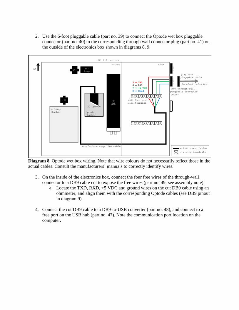
2. Use the 6-foot pluggable cable (part no. 39) to connect the Optode wet box pluggable

connector (part no. 40) to the corresponding through wall connector plug (part no. 41) on

the outside of the electronics box shown in diagrams 8, 9.

Diagram 8. Optode wet box wiring. Note that wire colours do not necessarily reflect those in the

actual cables. Consult the manufacturers’ manuals to correctly identify wires.

3. On the inside of the electronics box, connect the four free wires of the through-wall

connector to a DB9 cable cut to expose the free wires (part no. 49; see assembly note).

a. Locate the TXD, RXD, +5 VDC and ground wires on the cut DB9 cable using an

ohmmeter, and align them with the corresponding Optode cables (see DB9 pinout

in diagram 9).

4. Connect the cut DB9 cable to a DB9-to-USB converter (part no. 48), and connect to a

free port on the USB hub (part no. 47). Note the communication port location on the

computer.

(7) Pelican case

(1) Optode

(2)

GTD

up

bottom side

(51) Enclosed

wire terminal

1 2 3 4 5 6 7 8

1 2 3 4 5 6 7 8

(40) Through-wall

pluggable connector

(male)

= instrument cables

= wiring terminals#

To electronics box

(39) 6-ft

pluggable cable

5 = TXD

6 = RXD

7 = +5 VDC

8 = Grnd

(4)

Pump(5)

(6)

Manufacturer-supplied cable

Primary

chamber Optode

chamber

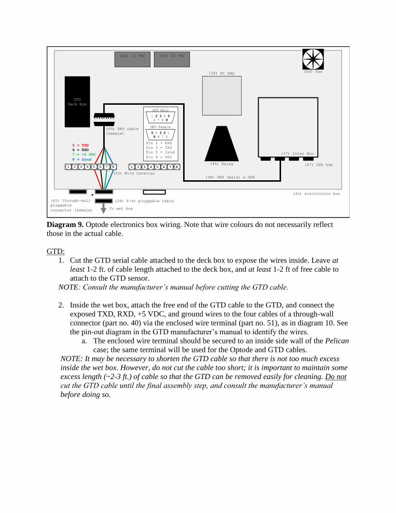
Diagram 9. Optode electronics box wiring. Note that wire colours do not necessarily reflect

those in the actual cable.

GTD:

1. Cut the GTD serial cable attached to the deck box to expose the wires inside. Leave at

least 1-2 ft. of cable length attached to the deck box, and at least 1-2 ft of free cable to

attach to the GTD sensor.

NOTE: Consult the manufacturer’s manual before cutting the GTD cable.

2. Inside the wet box, attach the free end of the GTD cable to the GTD, and connect the

exposed TXD, RXD, +5 VDC, and ground wires to the four cables of a through-wall

connector (part no. 40) via the enclosed wire terminal (part no. 51), as in diagram 10. See

the pin-out diagram in the GTD manufacturer’s manual to identify the wires.

a. The enclosed wire terminal should be secured to an inside side wall of the Pelican

case; the same terminal will be used for the Optode and GTD cables.

NOTE: It may be necessary to shorten the GTD cable so that there is not too much excess

inside the wet box. However, do not cut the cable too short; it is important to maintain some

excess length (~2-3 ft.) of cable so that the GTD can be removed easily for cleaning. Do not

cut the GTD cable until the final assembly step, and consult the manufacturer’s manual

before doing so.

GTD

Deck box

(39) 6-ft pluggable cable

(49) DB9 cable

(female)

(48) DB9 (male) x USB

5 = TXD

6 = RXD

7 = +5 VDC

8 = Grnd

(41) Through-wall

pluggable

connector (female)To wet box

DB9 Male

1 2 3 4 5

6 7 8 9

DB9 Female

5 4 3 2 1

9 8 7 6

Pin 2 = RXD

Pin 3 = TXD

Pin 5 = Grnd

Pin 9 = VDC

(53) Wire terminal

1 2 3 4 5 6 7 8(44) Relay

(37) Intel Nuc

(38) NI DAQ

(43) 24 VDC(42) 12 VDC

1 2 3 4 5 6 7 8(47) USB hub

(45) electronics box

(56) Fan

Diagram 10. GTD wet box wiring. Note that wire colours do not necessarily reflect those in the

actual cables.

3. Use the 6-foot pluggable cable (part no. 39) to connect the GTD wet box pluggable

connector (part no. 40) to the corresponding through-wall connector plug (part no. 41) on

the outside of the electronics box shown in diagrams 10, 11.

4. On the inside of the electronics box, connect the four free wires of the through-wall

connector to the corresponding TXD, RXD, +5 VDC and ground wires on the cut length

of cable extending from the GTD deck box. Join the cables via the wire terminal (part no.

53) as in diagram 11.

5. Connect the GTD deck box to a free port on the USB hub (part no. 47) using a DB9-to-

USB converter (part no. 48). Note the communication port location on the computer.

(7) Pelican case

(1) Optode

(2)

GTD

up

bottom

1 2 3 4 5 6 7 8

1 2 3 4 5 6 7 8

To electronics box

(39) 6-ft

pluggable cable

1 = TXD

2 = RXD

3 = +5 VDC

4 = Grnd

(4)

Pump(5)

(6)

(40) Through-wall

pluggable connector

(male)

(51) Enclosed

wire terminal

Primary

chamber Optode

chamberManufacturer-supplied cable

= instrument cables

= wiring terminals#

Diagram 11. GTD electronics box wiring. Note that wire colours do not necessarily reflect those

in the actual cables.

Ancillary components (flow meters and pump):

1. Cut a DB9 cable (part no. 49; see assembly note) to expose the wires inside. Cut both

pieces to ~2 ft. long. Insert the free ends of both cut cables through the cord grips (nos.

54, 55) mounted on the sides of the Pelican case (diagram 12) and electronics box

(diagram 13), respectively. The heads of the DB9 cable will face the outside of the wet

and electronics boxes.

2. Inside the wet box, connect the power and signal cables of the ancillary devices (pump

and flow meters) to the cut DB9 cable via an enclosed wire terminal (part no. 51)

mounted to the side of the Pelican case (diagram 12).

GTD

Deck box

1 2 3 4 5 6 7 81 2 3 4 5 6 7 8

1 = TDX

2 = RDX

3 = +5 VDC

4 = Grnd

To wet box

(48) DB9 (male) x USB(53) Wire terminal

(39) 6-ft

pluggable

cable

(41) Through-wall

pluggable

connector (female)

1 2 3 4 5 6 7 8(44) Relay

(37) Intel Nuc

(38) NI DAQ

(43) 24 VDC(42) 12 VDC

1 2 3 4 5 6 7 8(47) USB hub

(45) electronics box

(56) Fan

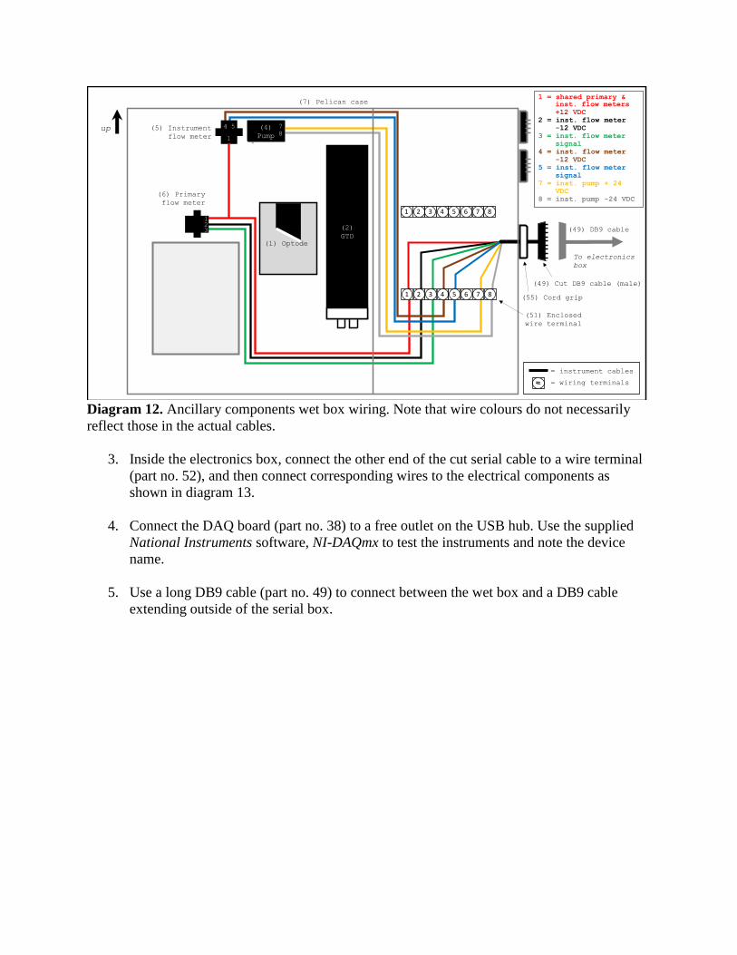
Diagram 12. Ancillary components wet box wiring. Note that wire colours do not necessarily

reflect those in the actual cables.

3. Inside the electronics box, connect the other end of the cut serial cable to a wire terminal

(part no. 52), and then connect corresponding wires to the electrical components as

shown in diagram 13.

4. Connect the DAQ board (part no. 38) to a free outlet on the USB hub. Use the supplied

National Instruments software, NI-DAQmx to test the instruments and note the device

name.

5. Use a long DB9 cable (part no. 49) to connect between the wet box and a DB9 cable

extending outside of the serial box.

To electronics

box

(4)

Pump(5)

(6)

4 5 7

8

123

(7) Pelican case

(4)

Pump

(1) Optode

(2)

GTD

up

1 2 3 4 5 6 7 8

1 2 3 4 5 6 7 8123

1

4 5 7

8

1 = shared primary & inst. flow meters

+12 VDC

2 = inst. flow meter

-12 VDC

3 = inst. flow meter

signal

4 = inst. flow meter

-12 VDC

5 = inst. flow meter

signal

7 = inst. pump + 24

VDC

8 = inst. pump -24 VDC

= instrument cables

= wiring terminals#

(49) DB9 cable

(55) Cord grip

(49) Cut DB9 cable (male)

(51) Enclosed

wire terminal

(5) Instrument

flow meter

(6) Primary

flow meter

Diagram 13. Ancillary components electronics box wiring.

Other wiring

1. Pass the AC power cables for the Nuc and the two DC power supplies through the wire

grip (part no. 54) on the side of the electronics box. Connect the cables to a power bar,

outlet or UPS.

2. Pass an HDMI cable through the wire grip to connect the computer monitor to the Nuc.

3. We recommend installing a small DC fan (part no. 56) on the side of the electronics box

to avoid over-heating. Connect the fan to a DC power supply (see diagram 14).

(44) Relay

(37) Intel Nuc

(38) NI DAQ

1 2 3 4 5 6 7 8

+ + -

4 7 8

13+

14-

A1

A2

3 (a/i 1 +)

2 (a/i 1 grnd)

a/o 0

5 (a/i 0 +)

4 (a/i 0 grnd)

(43) 24 VDC(42) 12 VDC

+ - -

1 2 4

+ -

7 8

1 2 3 4 5 6 7 8

1 = shared primary & inst. flow meters

+12 VDC

2 = inst. flow meter

-12 VDC

3 = inst. flow meter

signal

4 = inst. flow meter

-12 VDC

5 = inst. flow meter

signal

7 = inst. pump + 24

VDC

8 = inst. pump -24 VDC

(52) Wire terminal

(54) Wire grip

(49) Cut DB9 cable (female)

(49) DB9 cable

(47) USB hub

NI DAQ cable

1 2 3 4 5 6 7 81 2 3 4 5 6 7 8

(45) electronics box

(56) Fan

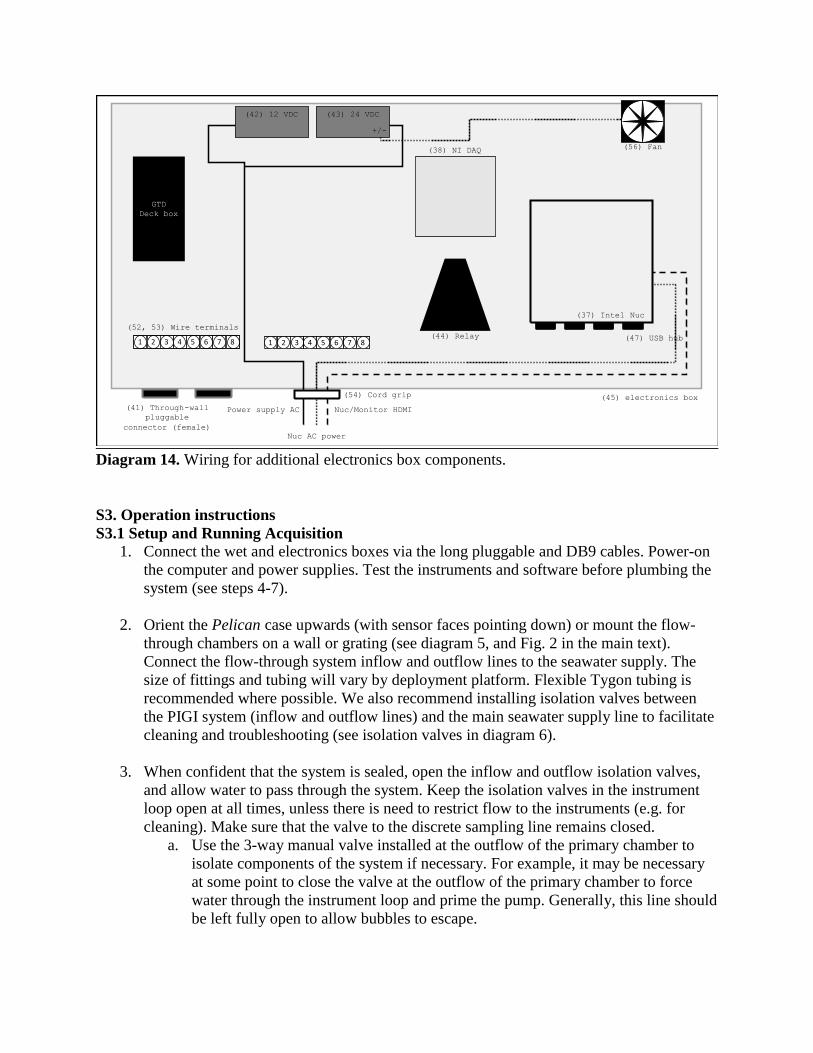
Diagram 14. Wiring for additional electronics box components.

S3. Operation instructions

S3.1 Setup and Running Acquisition

1. Connect the wet and electronics boxes via the long pluggable and DB9 cables. Power-on

the computer and power supplies. Test the instruments and software before plumbing the

system (see steps 4-7).

2. Orient the Pelican case upwards (with sensor faces pointing down) or mount the flow-

through chambers on a wall or grating (see diagram 5, and Fig. 2 in the main text).

Connect the flow-through system inflow and outflow lines to the seawater supply. The

size of fittings and tubing will vary by deployment platform. Flexible Tygon tubing is

recommended where possible. We also recommend installing isolation valves between

the PIGI system (inflow and outflow lines) and the main seawater supply line to facilitate

cleaning and troubleshooting (see isolation valves in diagram 6).

3. When confident that the system is sealed, open the inflow and outflow isolation valves,

and allow water to pass through the system. Keep the isolation valves in the instrument

loop open at all times, unless there is need to restrict flow to the instruments (e.g. for

cleaning). Make sure that the valve to the discrete sampling line remains closed.

a. Use the 3-way manual valve installed at the outflow of the primary chamber to

isolate components of the system if necessary. For example, it may be necessary

at some point to close the valve at the outflow of the primary chamber to force

water through the instrument loop and prime the pump. Generally, this line should

be left fully open to allow bubbles to escape.

GTD

Deck box

1 2 3 4 5 6 7 81 2 3 4 5 6 7 8

(33) Intel Nuc

Power supply AC Nuc/Monitor HDMI

Nuc AC power

+/-

1 2 3 4 5 6 7 8(44) Relay

(37) Intel Nuc

(38) NI DAQ

(43) 24 VDC(42) 12 VDC

1 2 3 4 5 6 7 8(47) USB hub

+/-

(41) Through-wall

pluggable

connector (female)

(54) Cord grip

(52, 53) Wire terminals

(45) electronics box

(56) Fan

4. Open the LabVIEW software library PIGI4.3_Library_2020.lib, and open the main

acquisition program autoPIGI_underway_2020.vi (Fig. S2). Alternatively, run the

autoPIGI_underway_2020.exe excecutable on the LabVIEW run-time engine. See section

S4 for details.

5. Start the program by clicking the run arrow in the LabVIEW program (see upper-left

corner of the window).

6. Check the deployment and control settings and data-save directories in the

autoPIGI_underway_2020 program, and confirm that the instrument communication

ports are set correctly (Fig. S3). Set the pump control mode to the desired manual or

automatic program. If using the automatic pumping program, specify the pumping rate

threshold for automatically turning off the seawater pump. Note that the main acquisition

program will save data continuously to a main storage location on the Nuc hard drive,

and to a secondary, external location. Check that the serial numbers for the Optode and

GTD instruments have been specified correctly; the LabVIEW acquisition reads the

Optode serial number from the data stream.

7. In the Automated Acquisition Restart Program panel (Fig. S6), set the desired time

interval between acquisition re-starts. This section of the program will automatically

restart the acquisition (i.e. clear the data figures and refresh the main acquisition) at a

user-defined interval to prevent a reduction in computer performance as data are stored in

LabVIEW cached memory.

8. Once the settings are correctly specified, click the blue "START ACQUISITION" button

to begin collecting data (Fig. S3). The program will first save the metadata and

instrument settings to separate files, before initiating the data collection and then

continuously reading, writing and plotting data. The automated restart countdown, which

controls the AutoIt software (see section S4 for details), will also begin once the

acquisition has been started.

NOTE: Do not click the "START ACQUISITION" button again as this will cause an

error with the automated re-start program.

9. If using the automatic pump control program, the instrument pump will turn on when the

acquisition begins. Otherwise, use the manual toggle on the front panel of the acquisition

program to turn on the pump (Fig. S3). The indicator on the screen will illuminate when

the pump is on. Adjust the flow rates if necessary by increasing/decreasing the voltage

output from the 24 VDC supply powering the instrument loop pump, as shown in Fig. S5.

10. When the automation restart countdown reaches the user-defined restart interval value,

the AutoIt program will automatically stop and then restart the acquisition program. Do

not use the mouse during this time.

11. At the end of the deployment, click the "STOP" or the red stop sign (upper right corner of

the window) buttons to end the data acquisition.

S3.2 End of acquisition and cleaning

1. At the end of a deployment, stop the LabVIEW program.

2. Turn off the flow of seawater through the instrument and close all of the isolation valves.

Disconnect the inflow and outflow tubing between the primary chamber and the ship’s

seawater supply lines.

3. Disconnect the cables between the wet box and electronics box.

4. We recommend flowing warm, freshwater through the system for ~5-10 minutes after

each deployment to minimize system wear. Clean the chambers and instruments,

following the example in the supplemental video (PIGI_Opt-chamber-cleaning.mp4).

a. Use the manual valves (part nos. 18, 19 and 26) to isolate different sections of the

system. It is possible to isolate and remove the primary and secondary chambers

separately for easy cleaning / maintenance.

b. Note that cleaning may be required during deployments in highly productive

waters with significant particulate loads.

S4. Description of additional files and software The PIGI system operates (collects, saves and displays data) through LabVIEW and autoIt

programs. Details of these programs, and Matlab scripts used to automatically process the data

are presented below. The software (including example output from the LabVIEW program and

corresponding output from the Matlab processing scripts) can be downloaded from:

github.com/rizett/PIGI_system.

NOTE: The main functions and scripts provided here were written by R. Izett. Additional

software not written by R. Izett are cited accordingly.

NOTE: Here and throughout, unless stated otherwise, we define gas saturation as the in-situ

seawater gas concentration, normalized to the temperature and salinity-dependent equilibrium

concentration at ambient sea level pressure and 0 dbar hydrostatic pressure. In the case of the

Optode read-out (e.g. Fig. S4), O2 saturation refers to the dissolved gas concentration

normalized to the temperature and salinity-dependent equilibrium concentration at 1 atm

standard atmospheric pressure and 0 dbar hydrostatic pressure. Temperature and salinity are

defined here as those values read by the Optode temperature sensor, and the constant /

hardwired Optode salinity value, respectively. Unless configured otherwise by the user, a value

of 0 PSU is used by the Optode; refer to the manufacturer's manual for details.

S4.1 LabVIEW

NOTE: The LabVIEW software provided here was written using LabVIEW 2019 (SP1)

development program. A license for this version, or newer, is required to open and modify the

provided scripts (see table S1). However, the free, stand-alone run-time engine (version 2019;

assembly note #26 in table S1) is sufficient to run the executable programs to perform

autonomous data acquisition. Run the installer to install our LabVIEW programs (descriptions

below) and the necessary run-time software and drivers. A description of the acquisition

workflow is provided in section S5, below, for operators who wish to develop alternative

software.

PIGI4.3_Library_2020: This package contains all of the LabVIEW programs required to run the

PIGI system (Fig. S2). The main programs are autoPIGI_underway_2020.vi and

PIGI_automation_restart.vi. Other sub-programs run individual components of the system.

Figure S2. The autoPIGI LabVIEW library. All of the LabVIEW programs used to communicate

with the instruments and log data are found within this library. The top three programs listed

(above the grey line) execute the main system functions and call sub-programs listed below).

NOTE: The descriptions of the files below are the same for versions run in the LabVIEW

development software and in the run-time engine program.

autoPIGI_underway_2020.vi or autoPIGI_underway_2020.exe: (Figs. S3, S4) This is the main

LabVIEW program used to interface with the PIGI system. The program acquires, logs and

displays data in real-time, and can be used to control the instrument loop pump. The data

headers in the output ascii data files (.lvm extension is a tab-delimited text file) are:

Computer Julian Day = Year-day time corresponding with the computer system time-stamp.

O2 saturation = Raw Optode percent saturation (%/100) at measured temperature and input

salinity.

O2 concentration = Raw Optode concentration (µmol L-1) at measured temperature and input

salinity.

Optode temperature = Water temperature (oC) measured by the Optode.

TDGP/GTD total dissolved gas pressure = Uncalibrated total dissolved gas pressure (mbar)

TDGP/GTD temperature = Temperature (oC) measured by the TDGP.

Instruments flow rate = Flow rate (L min-1) of water exiting the Optode chamber.

GPS Julian Day = Year-day time corresponding with the GPS system time-stamp (if

connected; 0 if not connected).

GPS Latitude = Latitude (oN) from the ship's GTD (if connected; 0 if not connected).

GPS Longitude = Longitude (oE) from the ship's GTD (if connected; 0 if not connected).

CalPhase = Optode raw CalPhase / Phase Shift (refer to manufacturer’s manual).

TC Phase = Optode raw TC Phase (refer to manufacturer’s manual).

c1rph = Optode raw c1rph (refer to manufacturer’s manual).

c2rph = Optode raw c2rph (refer to manufacturer’s manual).

c1_amp = Optode raw c1_amp (refer to manufacturer’s manual).

c2_amp = Optode raw c2_amp (refer to manufacturer’s manual).

opt_raw_T = Optode raw temperature (refer to manufacturer’s manual).

supply_V = TDGP voltage supply (refer to manufacturer’s manual).

ana1 = TDGP raw analog 1 (refer to manufacturer’s manual).

ana2 = TDGP raw analog 2 (refer to manufacturer’s manual).

dig1 = TDGP raw digital 1 (refer to manufacturer’s manual).

dig2 = TDGP raw digital 2 (refer to manufacturer’s manual).

Pump status = indicator if pump is on (1) or off (0).

Primary chamber flow rate = Flow rate (L min-1) of water exiting the primary chamber.

The main features of the program are:

a) Information and Notes (blue box in Fig. S3): Here, information about the deployment

can be recorded. For example, the Optode/GTD serial numbers and deployment details

can be recorded (note the required formats). This information is useful when post-

processing the data. The user will also specify the directory locations for saving data

files (“Save Path” and “Backup Save Path” objects).

b) User Control (red box in Fig. S3): In this section, the communication ports for the

instruments, and the system sampling rate can be set. The user can select to include a

GPS connection (via RS232). The “NI USB Dev. Name” refers to the name of the data

acquisition board (part no. 38 in Table S1).

c) Pump Control (green box in Fig. S3): In this section, users can select to manually or

automatically control the instrument pump. In the automatic mode, the pump will

automatically shut off when the flow rate falls below a user-defined threshold. If a

primary flow meter is installed, a threshold for both the primary chamber flow rate, and

instruments chamber flow rate can be set. The flow meter K-factors are scaling

coefficients unique to each meter and provided by the manufacturer.

d) Iridium Module (orange box in Fig. S3): Optional – Toggle the switch in the Iridium

section to the “off” position if not in use. If using the Iridium module, toggle to the “This

Computer” or “Other Computer” options, and set the “Iridium Save Path” to indicate

where a separate data file containing a subset of underway observations will be saved.

- Note that a second computer (“Other Computer” option), running the

“Send_iridium_standalone.vi” or “Send_iridium_standalone.exe” LabVIEW

program (Fig. S7), may be required for the Iridium module satellite transmitter

(part no. 57 in table S1) to have a clear view of the sky.

- Alternatively, place the PIGI electronics box near to a window, or use a patch

antenna to extend to a location with a clear view of the sky, and transmit the

iridium signal using the main LabVIEW program, autoPIGI_underway_2020.vi.

If the PIGI computer is being used to transmit the iridium signal (“This

Computer” option), adjust the settings in the “Transmit data via this computer”

box.

Figure S3. Front panel image of the autoPIGI_underway_2020 LabVIEW program. The

Information and Notes (blue), User Control (red), Pump control (green) and Iridium module

(orange) sections are shown.

NOTE: The stand-alone executable LabVIEW program, autoPIGI_underway2020.exe, begins on

start-up. The software provided for the base, full or professional development programs will only

begin after pressing the arrow key at the top right of the LabVIEW window. Starting this

program will not start the data acquisition; this must be completed after all of the settings in the

Information and Notes, User Control, Pump Control and Iridium Module sections have been

specified by the user. Once the settings have been updated, the user must click the blue "START

ACQUISITION" button to begin collecting data. This button should not be clicked again, unless

restarting the acquisition manually.

e) Data and Plots (Fig. S4): This section displays real-time gas and ancillary data signals.

Comments are saved to the data files in line with underway observations, and recorded

for post-processing. Startup or acquisition errors are displayed here. The "ERRORS" box

will illuminate in pink when an error has occurred. Most errors will terminate the

acquisition, but some (e.g. a failed iridium transmission) will simply display a warning.

The following data are displayed in separate tabs in this section:

- Gases %: Raw O2 saturation state and normalized GTD Pressure (i.e. GTD

pressure / 1013.25 mbar) (%)

- Raw Gases: Raw GTD pressure (mbar) and raw O2 concentration (µmol L-1)

- Ancillary: Temperature from the Optode and GTD (oC) and flow rates from the

primary and instrument flow meters (L/min)

o Note that the GTD temperature will likely read higher than the Optode as

the GTD head is not submerged in water.

o Note that the flow rate of the instrument pump can be adjusted by

changing the output voltage from the 24 VDC power supply (Fig. S5).

- Raw Signals: Raw data signals from the Optode and GTD (consult the

manufacturers’ manuals for details)

Figure S4. The data sections of the autoPIGI_underway_2020 LabVIEW program. Error

messages are also shown in this section.

Figure S5. Using a precision screwdriver, the voltage on the 12 VDC and 24 VDC can be

adjusted slightly (yellow circle). Turn clockwise to increase, and counter-clockwise to decrease.

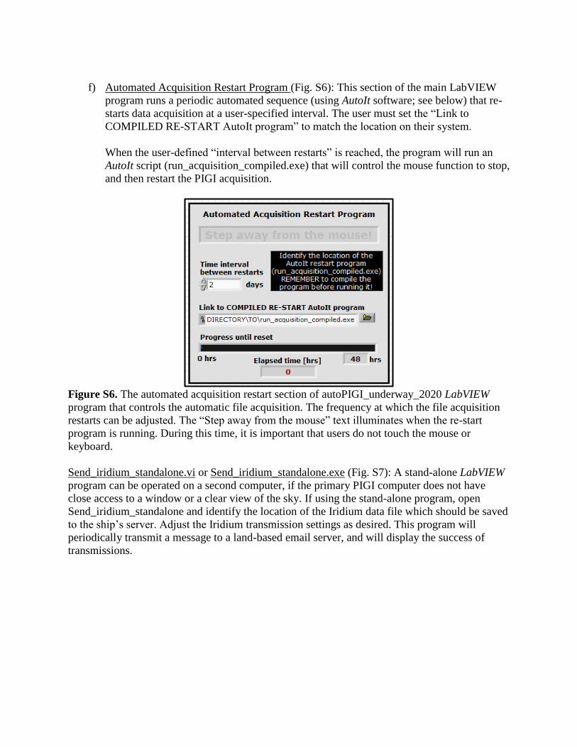
f) Automated Acquisition Restart Program (Fig. S6): This section of the main LabVIEW

program runs a periodic automated sequence (using AutoIt software; see below) that re-

starts data acquisition at a user-specified interval. The user must set the “Link to

COMPILED RE-START AutoIt program” to match the location on their system.

When the user-defined “interval between restarts” is reached, the program will run an

AutoIt script (run_acquisition_compiled.exe) that will control the mouse function to stop,

and then restart the PIGI acquisition.

Figure S6. The automated acquisition restart section of autoPIGI_underway_2020 LabVIEW

program that controls the automatic file acquisition. The frequency at which the file acquisition

restarts can be adjusted. The “Step away from the mouse” text illuminates when the re-start

program is running. During this time, it is important that users do not touch the mouse or

keyboard.

Send_iridium_standalone.vi or Send_iridium_standalone.exe (Fig. S7): A stand-alone LabVIEW

program can be operated on a second computer, if the primary PIGI computer does not have

close access to a window or a clear view of the sky. If using the stand-alone program, open

Send_iridium_standalone and identify the location of the Iridium data file which should be saved

to the ship’s server. Adjust the Iridium transmission settings as desired. This program will

periodically transmit a message to a land-based email server, and will display the success of

transmissions.

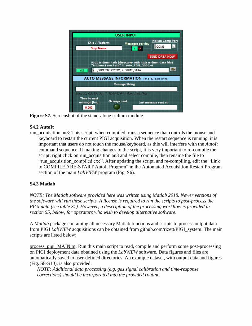
Figure S7. Screenshot of the stand-alone iridium module.

S4.2 AutoIt

run_acquisition.au3: This script, when compiled, runs a sequence that controls the mouse and

keyboard to restart the current PIGI acquisition. When the restart sequence is running, it is

important that users do not touch the mouse/keyboard, as this will interfere with the AutoIt

command sequence. If making changes to the script, it is very important to re-compile the

script: right click on run_acquisition.au3 and select compile, then rename the file to

“run_acquisition_compiled.exe”. After updating the script, and re-compiling, edit the “Link

to COMPILED RE-START AutoIt Program” in the Automated Acquisition Restart Program

section of the main LabVIEW program (Fig. S6).

S4.3 Matlab

NOTE: The Matlab software provided here was written using Matlab 2018. Newer versions of

the software will run these scripts. A license is required to run the scripts to post-process the

PIGI data (see table S1). However, a description of the processing workflow is provided in

section S5, below, for operators who wish to develop alternative software.

A Matlab package containing all necessary Matlab functions and scripts to process output data

from PIGI LabVIEW acquisitions can be obtained from github.com/rizett/PIGI_system. The main

scripts are listed below:

process_pigi_MAIN.m: Run this main script to read, compile and perform some post-processing

on PIGI deployment data obtained using the LabVIEW software. Data figures and files are

automatically saved to user-defined directories. An example dataset, with output data and figures

(Fig. S8-S10), is also provided.

NOTE: Additional data processing (e.g. gas signal calibration and time-response

corrections) should be incorporated into the provided routine.

\DIRECTORY\TO\IRIDIUM\DATA

NOTE: Additional ancillary datasets (e.g. sea surface temperature and salinity, and sea level

pressure) are required to run this script. Default values can be set, in the absence of real

observations.

pigi_processing.m: This sub-function reads and compiles all data from a single deployment.

optode_recalc.m: This sub-function re-calculates Optode O2 concentrations, saturation state and

partial pressure using updated sea surface temperature and salinity fields. The function uses the

Optode-specific foil coefficients (obtained from the manufacturer during multi-point sensor

calibration) to preform calculations.

n2_from_tp.m: This sub-function calculates N2 concentration and saturation from GTD total

dissolved gas pressure and Optode O2 measurements. ΔO2/N2 is also calculated.

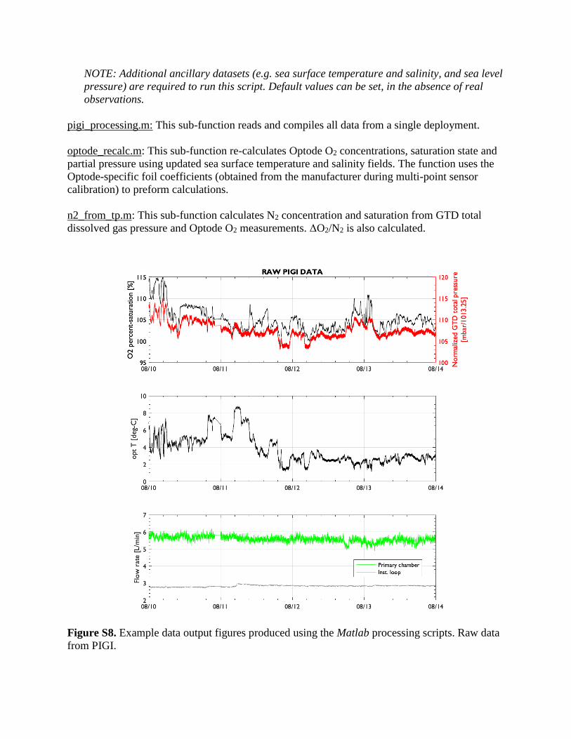
Figure S8. Example data output figures produced using the Matlab processing scripts. Raw data

from PIGI.

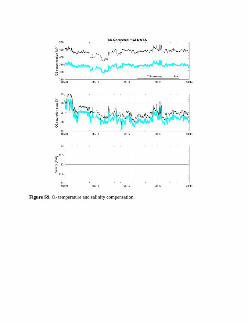
Figure S9. O2 temperature and salinity compensation.

Figure S10. Derived quantities.

S4.4 SolidWorks

Solidworks 3D CAD diagrams are at github.com/rizett/PIGI_system. A Solidworks license is

required to access these files. In the absence of a license, technical drawings of all parts are

provided in a separate file (PIGI4.3_Technical-drawings.pdf), and diagrams S1-S5 summarize

the designs presented in the CAD drawings.

S5. Acquisition and processing software workflow

As licenses are required to edit LabVIEW programs and run Matlab scripts (descriptions of these

files in section S4), we provide a workflow of key steps for operators who wish to develop their

own acquisition and processing programs using open-source software. The information presented

below is based on concepts of the system discussed in the main text, and can be used as a

template for developing future software versions.

S5.1 Acquisition

The following workflow diagram (Diagram 15) for data logging and acquisition should be

followed for optimal quality and post-processing efficiency. These principles are applied in the

software descriptions above (section S4).

Diagram 15. Workflow diagram for automated PIGI data acquisition. Thick black arrows

represent a progression of sequence; thin reversing black arrows represent a repeated sequence;

blue arrows imply data flow; green and red arrows represent true and false conditions,

respectively. Note that the Optode ancillary signals (e.g. CalPhase) and instrument settings are

required for most-accurate data post-processing. Refer to section S4.1 and Figs. S3, S4 above for

examples of these processes in our LabVIEW program.

S5.2 Data post-processing

The following workflow should be followed for post-processing and applying quality control

measures to the PIGI data. These principles are applied in the software descriptions above

(section S4).

1. Read and compile the PIGI data, including gas and ancillary measurements (flow rates,

temperature, and raw Optode/GTD signals).

2. Perform preliminary quality control checks:

a. Identify data obtained when the instrument pump was off.

Start sensor data

acquisition; turn ON

instrument pump

Save deployment

metadata and instrument

information (e.g. serial

nos.) as in Fig. S3

Read and save Optode

settings (see “get all”

function in

manufacturer's manual)

Set Optode and system

acquisition rate (see “set

interval function in

manufacturer's manual)

Re-start

acquisition

automatically

Run time = User-

defined restart

interval

User manually

stops acquisition

Stop

acquisition

Read Optode: parse O2

saturation, O2 concentration,

temperature, and raw signals

(e.g. CalPhase / Phase shift;

refer to manual for details)

Read GTD: parse dissolved gas

pressure, temperature and raw

signals (refer to manual for

details)

Save to data file

Update figures

Turn ON

instrument

pump

Turn OFF

instrument

pump

Primary chamber

flow rate >

threshold

AND

Instrument

chamber flow rate

> threshold

Read flow

rates

Read time / date

Read GPS

b. Identify data obtained when the flow rate through the instrument system was

below ~0.5 L min-1. Flow rates below this threshold result in a long residence

time in the instrument loop (>30 seconds) which could impact data quality in

highly-variable regions.

c. Check for data excursions: remove data outside of realistic ranges, which may

vary by deployment region.

3. Perform time-response corrections on gas and ancillary signals. The processing steps

below should be performed on aligned raw signals, including the raw instrument outputs

and ancillary measurements of temperature and/or salinity.

4. Re-calculate Optode O2 saturation state and concentrations.

a. Use underway salinity data to perform salinity compensation on the raw Optode

concentration. If underway temperature data were obtained from a TSG installed

near the PIGI system, use these data to recalculate the O2 concentration

following Uchida et al. (2008) as TSG temperature sensors are faster and more

accurate that the temperature sensor on the Optode. Use the Optode raw

CalPhase (Phase Shift) measurements, and the foil coefficients recorded to the

Optode settings file saved at the start of the underway acquisition.

b. Recalculate O2 saturation state using the salinity and most accurate temperature

data, and sea level pressure data. This can be acquired from reanalysis products

(e.g. NCEP/NCAR) or ship-board observations.

5. Adjust the TDGP total dissolved gas pressure data for bias.

a. Determine the offset between atmospheric pressure and TDGP measurements

made in air-equilibrated water or as in-air measurements. This should be

characterized at the start and end of each deployment.

6. Adjust the TDGP total dissolved gas pressure for warming between the seawater intake

and laboratory.

a. Seawater warming between the intake and point-of-measurement will induce gas

supersaturation. This can be approximated from the solubility equations of the

major gases (O2, N2, Ar) as the ratio of the equilibrium concentration at the water

temperature recorded at the seawater intake and the equilibrium concentration at

the water temperature recorded by the Optode/near the point of measurement. The

outside (true) sea surface temperature and degree of warming can be

approximated from CTD casts, or from an underway thermosalinograph installed

near to the seawater intake. The correction should be small, but will depend on the

degree of warming.

7. Calibrate the Optode using discrete samples analyzed by Winkler titration, or by periodic

in-air measurements.

8. Calculate N2 concentration, saturation (following McNeil et al., 2005) and ΔO2/N2 from

calibrated O2 and N2 saturation data, and ancillary temperature and salinity

measurements.

9. Manually remove data spikes and excursions.

References

McNeil, C., D. Katz, R. Wanninkhof, and B. Johnson. 2005. Continuous shipboard sampling of

gas tension , oxygen and nitrogen. Deep-Sea Research Part I, 52(9):1767–1785,

https://doi.org/10.1016/j.dsr.2005.04.003.

Uchida, H., T. Kawano, I. Kaneko, and M. Fukasawa. 2008. In situ calibration of optode-based

oxygen sensors. Journal of Atmospheric and Oceanic Technology, 25(12):2271–2281,

https://doi.org/10.1175/2008JTECHO549.1.