by

http://ssrn.com/abstract=1338787

Jan Eeckhout and Philipp Kircher

“Identifying Sorting - In Theory”

PIER Working Paper 09-007

Penn Institute for Economic ResearchDepartment of Economics University of Pennsylvania

3718 Locust Walk Philadelphia, PA 19104-6297

pier@econ.upenn.edu http://www.econ.upenn.edu/pier

Identifying Sorting - In Theory∗

Jan Eeckhout†and Philipp Kircher‡

January, 2009

Abstract

We argue that using wage data alone, it is virtually impossible to identify whether Assortative

Matching between worker and firm types is positive or negative. In standard competitive match-

ing models the wages are determined by the marginal contribution of a worker, and the marginal

contribution might be higher or lower for low productivity firms depending on the production func-

tion. For every production function that induces positive sorting we can find a production function

that induces negative sorting but generates identical wages. This arises even when we allow for

non-competitive mismatch, for example due to search frictions. Even though we cannot identify the

sign of the sorting, we can identify the strength, i.e., the magnitude of the cross-partial, and the

associated welfare loss. While we show analytically that standard fixed effects regressions are not

suitable to recover the strength of sorting, we propose an alternative procedure that measures the

strength of sorting in the presence of search frictions independent of the sign of the sorting.

∗We thank Rasmus Lentz, Jeremy Lise, Rafael Lopes de Melo, Giuseppe Moscarini and Fabien Postel-Vinay for insightful

discussions and comments. Kircher gratefully acknowledges support by the National Science Foundation, grant SES-

0752076, and Eeckhout by the ERC, Grant 208068.†Department of Economics, University of Pennsylvania and UPF, eeckhout@ssc.upenn.edu.‡Department of Economics, University of Pennsylvania and IZA, kircher@econ.upenn.edu.

1

1 Introduction

Sorting of workers to jobs matters for the efficient production of output in the economy. If there

are strong complementarities or substitutes between workers and jobs, the exact allocation has large

efficiency implications. In contrast, when complementarities are nearly absent, not much output is lost

from the random allocation of workers to jobs. This is important for policy, for example whether we

want to design an unemployment insurance program that provides incentives for workers to look for the

“right” job instead of accepting the first offer (see for example Acemoglu and Shimer 1999). There are

also profound implications for redistribution policies. In the presence of strong sorting, redistribution

through mismatching leads to substantial distortions whereas the distortions are minimal when sorting

is weak. And subsidies to education will in the presence of strong sorting lead to increased competition

between workers, thus transferring some of the subsidy rents from workers to firms.

Given the importance of sorting, a large body of recent empirical literature has estimated whether

sorting is positive or negative. In part, this renewed interest has been catalyzed by the availability

of worker-firm match data. Several empirical papers (Abowd, Kramarz, and Margolis (1999), Abowd,

Kramarz, Lengermann, and Perez-Duarte (2004)) find an insignificant or even negative correlation in

fixed effects between worker and firm types. This result has been replicated for a number of countries

such as France, US, Denmark and Brazil. The result is taken as indication that Positive Assortative

Matching between workers and firms does not play a role in the labor market.

On the other hand, recent work reveals that a structural labor search model that has strong com-

plementarities and thus induces Positive Assortative Matching in equilibrium can nevertheless generate

smaller and even negative correlations in the fixed effects of workers and firms (Gautier and Teulings

(2006), Lise, Meghir and Robin (2008), Lopes de Melo (2008) and Lentz (2008)). In some cases this

is attributed to the non-linear structure of the wage setting that is not picked up in the regression

specification. Other work by Gabaix and Landier (2008) argues that sorting of CEOs has become more

important as is reflected in the increased wages.

In this paper we address the issue of identification of sorting in a simple theoretical framework and

obtain the following results. First, in the frictionless matching model (Becker 1973), we show that

identifying whether sorting is positive or negative is impossible using wage data alone. To see this, note

that in this model more productive workers always earn higher wages and more productive firms always

make more profits. Under Positive Assortative Matching (PAM), the more productive firm also has

the highest marginal product from labor, i.e. the cross-partial is positive. This implies that high type

firms hire high type workers and they pay high wages. Under Negative Assortative Matching (NAM)

instead, low productive firms have a comparative advantage from hiring more productive workers, i.e.

2

the cross-partial is negative.1 As a result, high type firms pay lower wages. By ranking firms according

to the wages they pay, we do not identify the most productive firm. Without any additional data on

the profitability of each job, it is impossible to identify whether sorting is positive or negative. This is

true even if we consider wages off the equilibrium path.

Second, we explicitly allow for mismatch to occur in equilibrium due to search frictions. We find

that the first-order effect is that wages of a given worker have an inverse U-shape around the optimal

allocation, the “bliss point”. Under mismatch with a relatively bad firm, wages increase as the firm

type increases because the firm moves closer to the bliss-point, whereas wages decrease once the worker

is mismatched with too good a firm because better firms move further from the bliss-point. Higher

productivity firms have to be compensated for their willingness to match with a “bad” worker because it

destroys their opportunity to match with a “good” worker. This leads to the bliss-point in the pattern

of compensation if a worker meets the “right” firm, rather then a wage schedule that is increasing

everywhere in the type of firm. The net effect on a given worker’s wages from increasing the firm

type is therefore ambiguous and second-order. For the simplest, type-independent cost of delay, we

explicitly show that the net effect is exactly equal to zero under some common specification. This

version, also studied in Atakan (2006), is a close reformulation of Becker (1973). When search costs

are type-dependent (as in Shimer and Smith (2000) for example), the net effect may still be either

positive or negative. The additional component induced through type-dependence is proportional to

the magnitude of the friction and, compared to the inverted U-shape, the net effect of firm type on

wages is likely to be second-order and difficult to isolate in the data.

Third, and in spite of the fact that we cannot identify the sign, we develop a method that in theory

allows for identification of the strength of sorting. Ultimately, efficiency properties depend on how big

the complementarities/substitutes are. Identification derives from the distinct features of the range

of wages a worker receives who has been observed repeatedly. First, the highest wage corresponds to

her bliss-point. We use this to order the workers and obtain the type distribution. Likewise, we can

obtain an order of the firms by the level of wages that they pay (this identifies those firms with the

highest willingness to hire better workers - which is positively related to type under positive sorting

and negatively under negative sorting). Second, the difference between the highest and the lowest wage

is equivalent to the cost of search. Third, we calculate the loss due to mismatch over the range of

wages, which from the theory can be expressed in terms of the absolute value of the cross-partial of

the production function. Given that we know the cost of search, we can now obtain the strength of the

cross-partial, or equivalently, the strength of sorting.1We use the term comparative advantage to denote a larger absolute gain in output from matching with a better

worker, rather than the stronger concept of a larger percentage gain as used e.g. in Sattinger (1975).

3

Before proceeding to the model, we briefly lay out the empirical issue. Abowd, Kramarz, and

Margolis (1999) use a simple empirical measure of sorting that can be obtained by estimating a log-wage

equation in which wages are a function of a worker fixed effect, a firm fixed effect, and an orthogonal

error term

logwit = aitβ + δi + ψj(i,t) + εit (1)

where wit denotes the wage, ait are time varying observables of workers, δi is a worker fixed effect, ψj is

the fixed effect of the firm j at which worker i is employed at time t, and εit is an orthogonal residual.

That is, ψj captures the average effect that a firm has on the wages of the workers that are willing

to match with it. The correlation between αi and ψj in a given match is taken as an estimate of the

degree of sorting. Abowd et al (2004) propose a bargaining procedure in which higher firms pay higher

wages in line with (1) as a test of Becker’s (1973) idea of matching.

We argue here that such a pay schedule is inconsistent with Becker’s theory because every worker

would like to match with the best firm. Becker’s theory is inseparably linked to a theory of wages

which prevents such overcrowding of workers at top firms. We point out the distinctive features of the

underlying theory of wages, and extend them to a simple and tractable model with search frictions. We

show in our theoretical exercise that the assumption that the firm effect is independent of the worker’s

type is theoretically not justified in this setting. In particular, for those workers who are matched with

a firm that has a lower rank than their own, the wage increases when the firm type increases because

the worker-firm “fit” improves. In contrast, workers who are matched with a lower ranked firm see a

decrease in the wage when the firm becomes better because the worker-firm “fit” deteriorates.

A similar logic holds in the context of matching with frictions. With wage bargaining in a model

with search frictions, the set of eligible partners is bounded by those matches where the match surplus

is zero relative to continue searching. For all acceptable partners the surplus is positive. For a given

worker type, the surplus goes to zero for a match both with too bad a firm and too good a firm. Any

bargaining procedure that pays wages that are monotonic in the surplus will therefore result in wages

being non-monotonic in firm type.

The goal of our analysis is to lay out this logic in the simplest possible environment. First, we

consider the frictionless benchmark, and then we extend it in a straight-forward way to a model with

frictions that allows worker and firm mismatch. Frictions are modeled in a two-stage set up: a stage of

random matching is followed by a frictionless matching stage. The benefit of our modeling approach is

that the main effects that drive the wage determination become clearly visible and highlights the forces,

limitations, and possibilities that arise in estimations that are based solely on wage data. As such, it

informs our understanding of the results obtained in more complicated infinite horizon steady-state

models that preclude closed-form theoretical analysis but are often used for structural estimation.

4

2 The Frictionless Model

In order to make our point we start with the following very simple matching model following Becker

(1973). There is a unit mass of worker and a unit mass of firms. Workers and firms are heterogeneous

in terms of their productivity. Workers draw their type x from distribution Γ(x) with smooth density

γ(x) on [0, 1]. Firms draw their type y from distribution Υ(y) with smooth density υ(y) on [0, 1].

When types x and y form a match, they produce positive output f(x, y) > 0 whilst having an

outside option of remaining unmatched. We assume that workers and firms can be ranked in terms

of their productivity, i.e. fx > 0 and fy > 0. Then it is without loss of generality to index a worker

by his rank in terms of productivity, i.e. by the fraction of workers that are less productive then him.

Similarly, we can identify each firm by its rank in the distribution of firm productivities. This means

that Γ(.) = Υ(.) = x, i.e. the distributions are uniform.2 Assume that workers who do not get matched

obtain a payoff of zero, and since output is non-negative, all agents will prefer to match. If output

of all matches is strictly positive, there will be a continuum of wage schedules that can support the

same allocation, and we will assume that an exogenous bargaining procedure determines which split of

surplus is implemented. We will denote this payoff by the constant w0 ≥ 0 that pins down the wage of

the lowest worker type.

For the assignment of workers to firms the cross-partial of the production function is important.

We do not restrict the sign of the cross-partial since this will be instrumental in determining whether

there is positive or negative assortative matching. Denote by F be the class of all functions f that

are monotonic: fx, fy > 0; and that have a monotonic marginal product: fxy(x, y) is either always

positive or always negative.3 The assumption that the cross-partial does not change sign allows us to

unambiguously talk about positive or negative sorting. Production functions for which higher worker

types always have a comparative advantage at better firms (fxy > 0) are in set F+ ⊂ F . Production

functions for which higher worker types always have a comparative advantage at lower firms (fxy < 0)

are in set F− ⊂ F .

To illustrate the implications of our analysis we will derive our results for the following examples of

production functions

f+(x, y) = αxθyθ + h(x) + g(y), (2)

f−(x, y) = αxθ(1− y)θ + h(x) + g(y), (3)2The uniformity assumption is without loss of generality since the production function can be identified only up to a

normalization: For a general Γ(·) and Υ(·) and f(·, ·) we can alternatively consider a uniform type space in which only

the ranking matters and an alternative production function f(x, y) = f(Γ(x), Υ(y)).3Later, in section 5 we discuss the virtues of relaxing this assumption.

5

where g(.) and h(.) are increasing functions and α ≥ 0 and θ > 0 are parameters that indicate the

strength of the complementarities. We assume that g(y) is such that higher firms produce higher

output even under the second specification. It is obvious that f+ ∈ F+ and f− ∈ F−.

An assignment of workers x to firms y is denoted by µ, i.e., the partner y of worker x is µ(x).

In this part of the paper we assume a competitive matching market. A market equilibrium specifies

an assignment between x’s and y’s and some wage schedule w(x, y) ≥ w0 that determines the split of

output between the worker and the firm. The payoff to the worker is w(x, y) and the payoff to the

firm is π(x, y) = f (x, y) − w(x, y) ≥ 0. Both workers and firms take the wage schedule as given. The

tuple of functions (µ,w) is an equilibrium if no worker wants to switch to a different firm at the market

wages, i.e.

w(x, µ(x)) ≥ w(x, y) for all x and y;

and no firm wishes to employ a different worker, i.e.

π(µ−1(y), y) ≥ π(x, y) for all x and y.4

We derive the main prediction of Becker’s (1973) model concerning the wages in the economy. In

equilibrium, each firm y maximizes profits, taking the wage schedule as given:

maxx

f(x, y)− w(x, y).

This yields the first order condition

fx(x, y)− dw(x, y)dx

= 0. (4)

Let w?(x) be the equilibrium wage of worker x. Integrating (4) along the equilibrium path yields

w?(x) =∫ x

0fx(x, µ(x))dx+ w0, (5)

where the constant of integration is pinned down by w0. Observe that the worker obtains exactly his

marginal product along the equilibrium allocation. Therefore, equilibrium profits of type y are given

by output minus the wage w? with the optimal worker µ−1(y). This can be re-written as

π?(y) =∫ y

0fy(µ−1(y), y)dy + f(0, 0)− w0 (6)

Furthermore, we know from Becker’s analysis that matching is positive assortative when the production

function is supermodular (fxy > 0), in which case µ(x) = x. Under submodularity (fxy < 0) in

4It is well-known that a strict cross-partial yields a one-to-one mapping µ(·) in equilibrium. In general µ(·) is a

correspondence, with the equilibrium definition extended to all pairs in that correspondence.

6

equilibrium the matching is negative assortative and µ(x) = 1 − x. With this in mind, we show that

in this simple competitive model the direction of sorting - i.e. the sign of the cross-partial - cannot

be identified from wage data. We first show this result on the equilibrium path, then we show it off

the equilibrium path. In the next section we build an extended model with search frictions where the

wages off the equilibrium path actually arise.

2.1 On the equilibrium path

We will first illustrate the result by considering our restricted class of production functions outlined

above and then present the general theorem. Suppose the underlying production technology is not

known and the true technology is either one of the two example technologies f+ given in (2) or f−

given in (3). By (5) the wages under f+ are

w∗(x) =∫ x

0f+

x (x, x)dx+ w0

=∫ x

0

(αθx2θ−1 + hx(x)

)dx+ w0 =

α

2x2θ + h(x)− h(0) + w0.

Under f−, the equilibrium wages are

w∗(x) =∫ x

0f−x (x, 1− x)dx+ w0

=∫ x

0

(αθx2θ−1 + hx(x)

)dx+ w0 =

α

2x2θ + h(x)− h(0) + w0.

Under both functions the wages on the equilibrium path are exactly identical, and from wage data

alone one cannot distinguish between positive and negative sorting. The problem is obtaining the order

of the firms. If we only have wage data and no profit data, and we derive the order on the firms by

ranking them by increasing wages, we will obtain two different orders depending on whether we have

complements or substitutes. To see this, observe that under positive assortative matching (henceforth

PAM) higher type firms pay higher wages along the equilibrium path whereas under negative assortative

matching (NAM) higher type firms pay lower wages. In the former w(y, y) = αy2θ

2 is increasing in y,

in the latter w(1 − y, y) = α(1−y)2θ

2 is decreasing in y. This result is true for any general production

technology as summarized in the proposition that follows below.

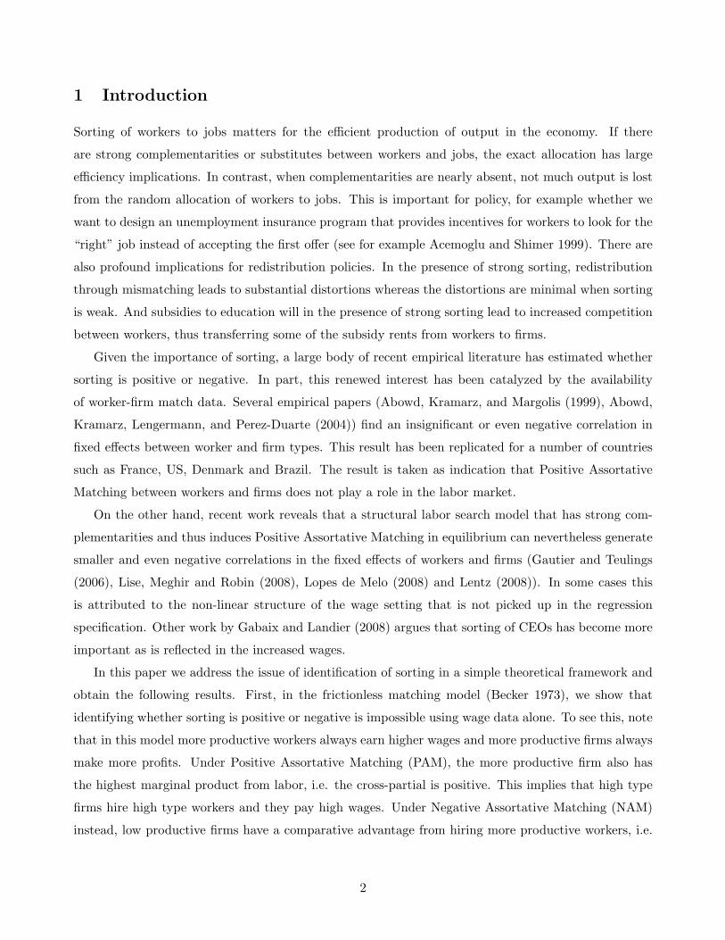
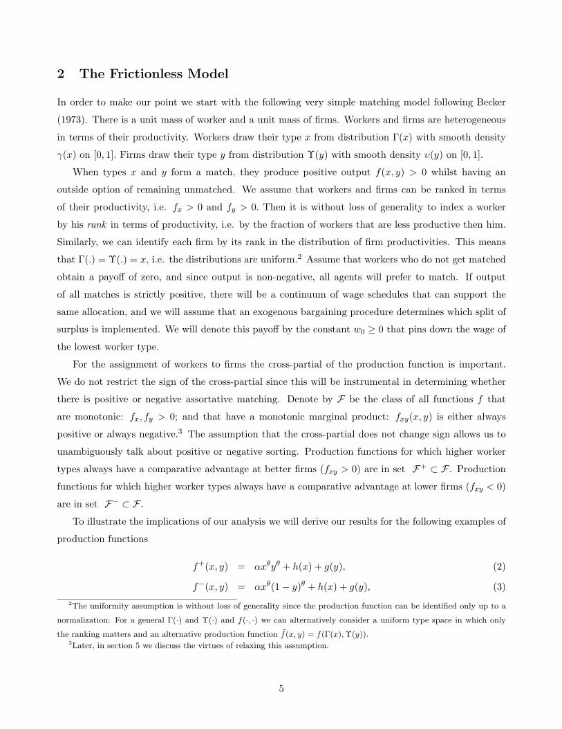
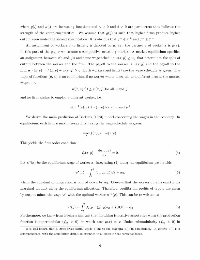
Figure 1 has an example with the profits, wages and total output when f+ = xy+y and f− = x(1−

y) + y. Observe that wages are identical in both cases (blue), but that profits are decreasing in worker

type x under f+. While higher y firms have higher profits, higher x workers are matched with lower y

firms who obtain lower profits. In the example, with w0 = 0, we obtain w+(x, µ(x)) = x2

2 , π+(x, µ(x)) =

x2

2 + x, f+(x, µ(x)) = x+ x2 and w−(x, µ(x)) = x2

2 , π−(x, µ(x)) = x2

2 + 1− x, f+(x, µ(x)) = 1− x+ x2.

7

10.750.50.250

2

1.5

1

0.5

0

x

f,w,pi

2

10.750.50.250

2

1.5

1

0.5

0

x

f,w,pi

1

Figure 1: Equilibrium Wages w(x, µ(x)) [blue lines], Profits π(x, µ(x)) [green lines], Total Output

f(x, µ(x)) [red lines] under f+ = xy + y [left] and f− = x(1− y) + y [right] with w0 = 0.

Of course, under NAM π?,−(y) = y + (1−y)2

2 is increasing in y even though π−(x, µ(x)) is decreasing in

x. Profits will not be the same under both production functions.

Proposition 1 For any production function f ∈ F+ that induces positive sorting there exists a pro-

duction function f ∈ F− that induces negative sorting and the equilibrium wages w∗(x) are identical

under both production functions.

Proof. ¿From equation (5) we obtain the wage schedule. When generated by an underlying production

process that is supermodular f+ this is

w?,+(x) =∫ x

0f+

x (x, x)dx+ w+0 ,

and for a submodular process f− it is

w?,−(x) =∫ x

0f−x (x, 1− x)dx+ w−

0 .

Observe that since w?,+(0) = w+0 and w?,−(0) = w−

0 , both wage schedules are identical when the free

bargaining paramter satisfies w+0 = w−

0 = w0 as we assumed. Then for w?,+(x) = w?,−(x) for all x, it is

sufficient that f+x (x, x) = f−x (x, 1− x). For any f+(x, y) on [0, 1]2 we can define f−(x, y) = f+(x, 1−y)

on [0, 1]2. The only restriction is that this function may not be increasing in y, so we may need to

“augment” the function to ensure that fy is positive. If fx, fy are bounded, it is sufficient to add a term

τ · y where τ > 0 is large enough to ensure fy > 0 everywhere. If fy is not bounded and negative, we

need to add a function g(y) that increases faster than the decrease of f+(x, 1− y) in y.

8

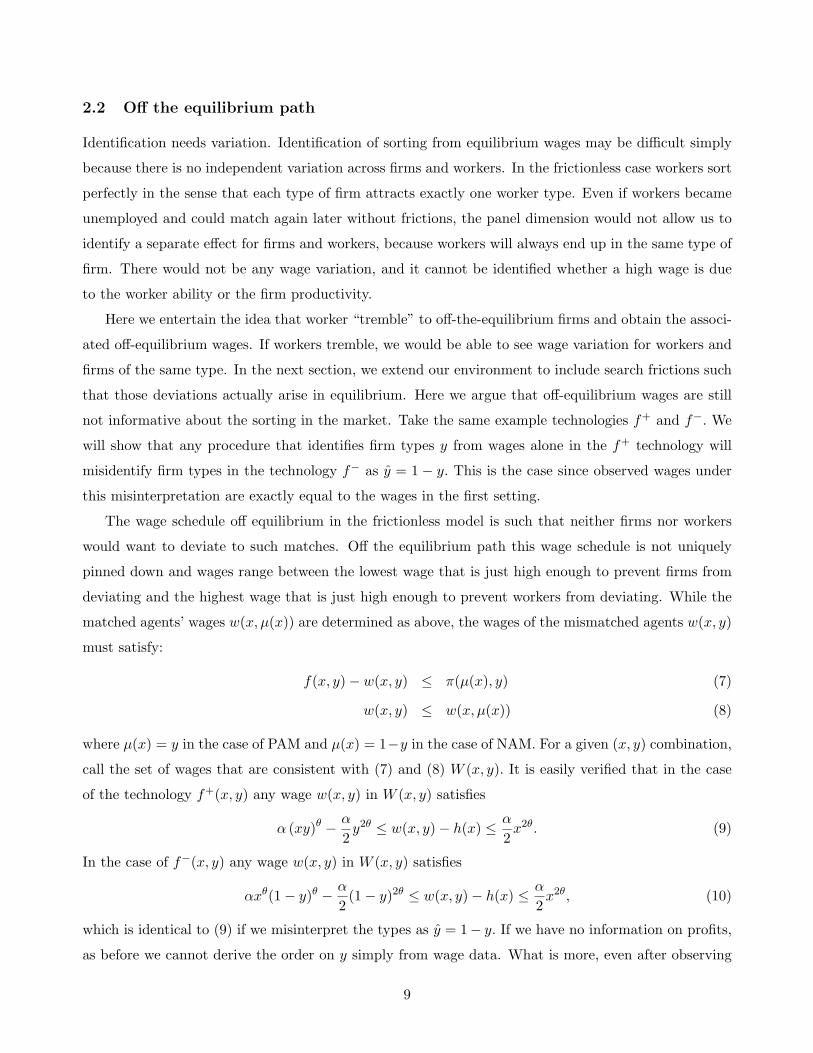
2.2 Off the equilibrium path

Identification needs variation. Identification of sorting from equilibrium wages may be difficult simply

because there is no independent variation across firms and workers. In the frictionless case workers sort

perfectly in the sense that each type of firm attracts exactly one worker type. Even if workers became

unemployed and could match again later without frictions, the panel dimension would not allow us to

identify a separate effect for firms and workers, because workers will always end up in the same type of

firm. There would not be any wage variation, and it cannot be identified whether a high wage is due

to the worker ability or the firm productivity.

Here we entertain the idea that worker “tremble” to off-the-equilibrium firms and obtain the associ-

ated off-equilibrium wages. If workers tremble, we would be able to see wage variation for workers and

firms of the same type. In the next section, we extend our environment to include search frictions such

that those deviations actually arise in equilibrium. Here we argue that off-equilibrium wages are still

not informative about the sorting in the market. Take the same example technologies f+ and f−. We

will show that any procedure that identifies firm types y from wages alone in the f+ technology will

misidentify firm types in the technology f− as y = 1 − y. This is the case since observed wages under

this misinterpretation are exactly equal to the wages in the first setting.

The wage schedule off equilibrium in the frictionless model is such that neither firms nor workers

would want to deviate to such matches. Off the equilibrium path this wage schedule is not uniquely

pinned down and wages range between the lowest wage that is just high enough to prevent firms from

deviating and the highest wage that is just high enough to prevent workers from deviating. While the

matched agents’ wages w(x, µ(x)) are determined as above, the wages of the mismatched agents w(x, y)

must satisfy:

f(x, y)− w(x, y) ≤ π(µ(x), y) (7)

w(x, y) ≤ w(x, µ(x)) (8)

where µ(x) = y in the case of PAM and µ(x) = 1−y in the case of NAM. For a given (x, y) combination,

call the set of wages that are consistent with (7) and (8) W (x, y). It is easily verified that in the case

of the technology f+(x, y) any wage w(x, y) in W (x, y) satisfies

α (xy)θ − α

2y2θ ≤ w(x, y)− h(x) ≤ α

2x2θ. (9)

In the case of f−(x, y) any wage w(x, y) in W (x, y) satisfies

αxθ(1− y)θ − α

2(1− y)2θ ≤ w(x, y)− h(x) ≤ α

2x2θ, (10)

which is identical to (9) if we misinterpret the types as y = 1− y. If we have no information on profits,

as before we cannot derive the order on y simply from wage data. What is more, even after observing

9

off-the-equilibrium path wages, the bounds on the wages under PAM and NAM are identical if we use

the order on wages to derive the order on y (in which case under NAM we assign the order 1− y to the

firms). The static Beckerian model will therefore not allow for identification of assortative matching

based on wage data alone.

Proposition 2 For any production function f ∈ F+ that induces positive sorting there exists a pro-

duction function f ∈ F− that induces negative sorting and the equilibrium wage sets W (x, y) in the

former are identical to equilibrium wage set W (x, 1− y) in the latter.

Proof. The proof follows the same argument as in Proposition 1.

3 Mismatch due to Search Frictions

We now consider an extended model with mismatch due to frictions caused by delay. Unlike the static

Beckerian model, search frictions may induce different behavior in the acceptance decision of matches.

First, assuming that the technology is generated by a supermodular production technology, we derive

the equilibrium allocation in the presence of a type-independent search cost. We address the issue

of identification of positive/negative sorting in this model, and whether we can identify sorting from

wage data alone. Second, for this model we derive from the theory the firm-fixed-effect. The case of

type-independent search costs considerably simplifies the analysis, but the gist of the argument carries

over for a more general search cost. Below in section 5 we consider a model with type-dependent search

cost.

3.1 Type-Independent Search Costs Under Supermodularity

Our model has hiring in two stages. In stage one, each worker is randomly paired with one firm. The

pairings are random. One can think of this part of the hiring process as standing in for some connections

that workers have to the labor market prior to engaging in an extensive search for labor. The pair can

either agree to stay together at some wage, or search for a better partner. Those who decide not to

stay together and those who did not get paired each incur a search cost c due to the delay. In the

second stage, all remaining agents are matched according to the competitive, frictionless allocation as

outlined above.5 After the search process has ended production starts. To allow for a panel dimension5Here we need to worry about the possibility that when the acceptance sets span the entire type space (e.g. because of

high search costs or low complementarities), no agents are left in the second stage, in which case the continuation payoff is

not determined. Without modeling this explicitly, we think of a tremble that ensures that there are always some agents

who end up in the next period. For many parameters each worker and firm type rejects some agents on the other side of

the market, and these agents will indeed move to the second stage.

10

in the observations (i.e. each worker matched over time to more than one firm, and each firm matched

over time with more than one worker) we assume that each agent goes through this two-stages hiring

process several times in his life.6

We consider the same class of production functions F . For exposition it will be convenient to

restrict the supermodular function in F+ to functions with symmetric cross-partial such that fxy(x, y) =

fxy(y, x). For submodular functions in F− which induce negative sorting it will be convenient to restrict

attention to symmetry of the form fxy(x, y) = fxy(1− y, 1− x).

We assume that the transfer in the first period is determined by Nash bargaining with equal bar-

gaining weights. We illustrate this with our example production function f+ in (2). When a worker

x meets a firm y, the payoff from matching is f(x, y). Waiting until next period and matching in the

perfectly competitive labor market yields payoff w(x, µ(x)) − c to the worker and π(µ−1(y), y) − c to

the firm. A first-period match will therefore be accepted provided that the current match surplus over

waiting is positive7 , i.e.

f(x, y)− (w∗(x) + π∗(y)− 2c) ≥ 0. (11)

For a given firm y we call the set of worker types that fulfill (11) his acceptance set and denote it by

a(y).8 Similar to the work by Atakan (2006) we can show that the bounds of this set are increasing if

the production function is in F+ and decreasing if it is in F−, which naturally extends the notion of

sorting to sets.

For our example production function f+ in (2) it is easy to verify that (11) reduces to

α(xy)θ − α

2x2θ − α

2y2θ ≥ −2c. (12)

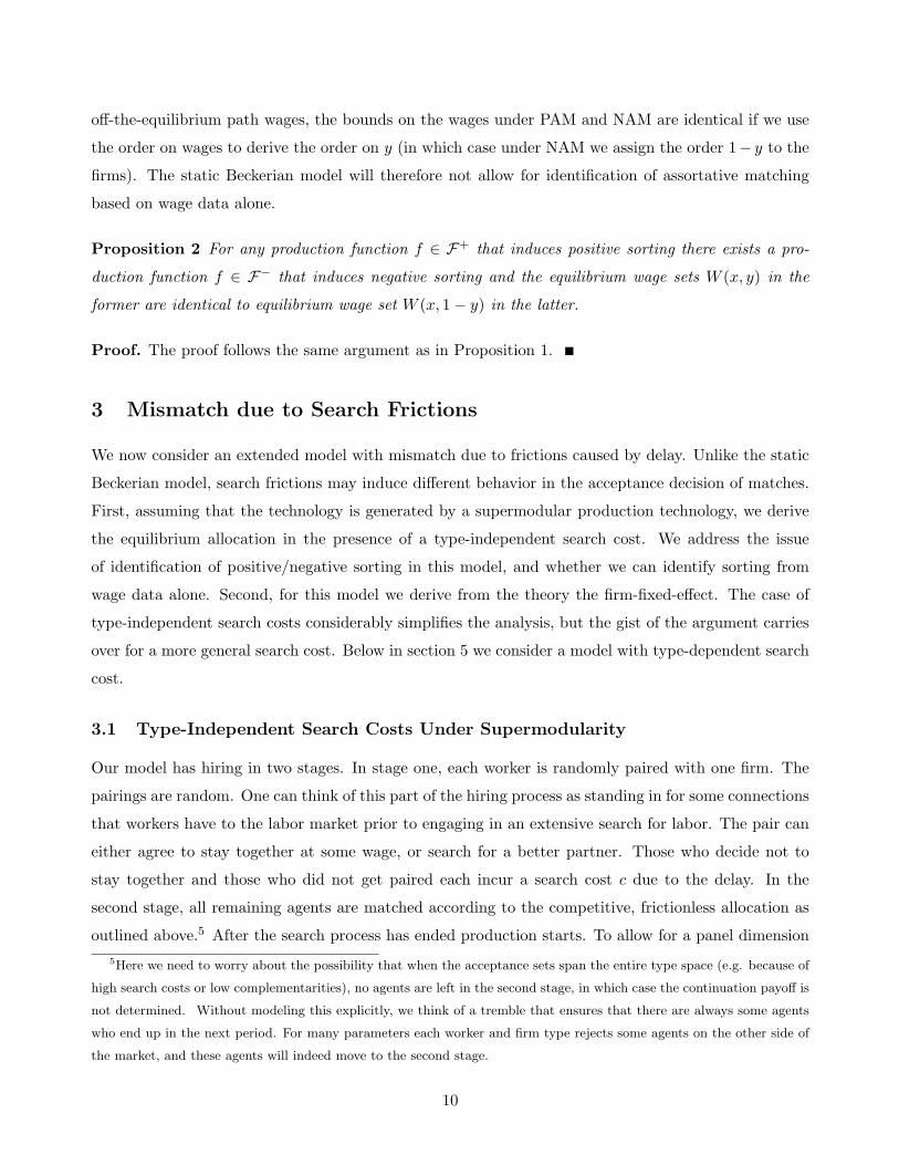
and therefore the acceptance set becomes

a(y) =[(yθ − 2

√c/α)1/θ, (yθ + 2

√c/α)1/θ

]. (13)

6One can think of termination of all jobs after a specified time period, with a new period of matching that follows.

More generally one may think of this as standing in for exogeneous separations into a steady state matching model.7It may well be that for low types the surplus in the next period does not exceed the total waiting cost of 2c. In order

to avoid keeping track of endogenous entry, we assume that people will search even if that is the case. This may be due to

the fact that the outside option (e.g. unemployment benefits) are contingent on searching. This issue never arises when

f(0, 0) > c and w0 > c, as all agents than have an incentive to search, or when search costs are proportional as in Section

5.8Note that for supermodular functions in F+ this acceptance set is identical for workers and firms of the same type

types, which is a general consequence of the symmetry of fxy. Therefore the distribution of types in the second stage

is identical for workers and firms, and therefore the equilibrium assignment is still µ(x) = x. Similarly, for submodular

functions in F− is can be shown that under our symmetry condition when x accepts y then 1 − x accepts 1 − y, which

leads to distributions that are symmetric around 1/2 (1 − Γ(x) = Γ(1 − x), 1 − Υ(y) = Υ(1 − y)) and the equilibrium

assignment indeed remains µ(x) = 1 − x.

11

x

y

2√

c

10

1

Figure 2: Acceptance sets with type-independent search costs for θ = 1.

The matching sets are illustrated in Figure 2 for the case θ = 1.

Because the surplus is divided equally, the worker obtains half of this surplus on top of his outside

option that is given by his value of waiting. Therefore, his wage is

w(x, y) =12[f(x, y)− w(x, µ(x))− π(µ−1(y), y) + 2c

]+ w(x, µ(x))− c (14)

=12[f(x, y) + w(x, µ(x))− π(µ−1(y), y)

]. (15)

It is straightforward to see that this wage is exactly in the middle of the acceptance set W (x, y)

outlined in (7) and (8) for off-equilibrium-wages of the frictionless model. This makes this model

very attractive to work with. It translates the insights from Becker’s (1973) assignment model to a

model of mismatch. It immediately implies that positive and negative sorting cannot be identified by

observed wage data, because the wages under supermodular production functions coincide with those

under submodular production functions (under misinterpretation of the unobserved firm type). Since

the wage distributions coincide, the identification cannot come from the acceptance decisions (i.e. the

speed of matching) between first and second period, either, because identical wages imply identical

acceptance decisions (again under the misinterpretation of firm types).9

9Bargaining weights different from 1/2 or different costs for workers and firms will change the bargaining sets and the

wages, but it can be shown that they will not affect our results on identification as long as search costs are identical for

all workers and for all firms.

12

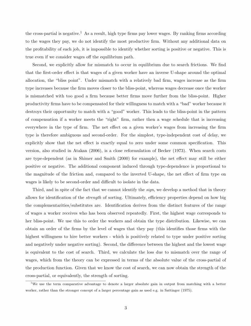
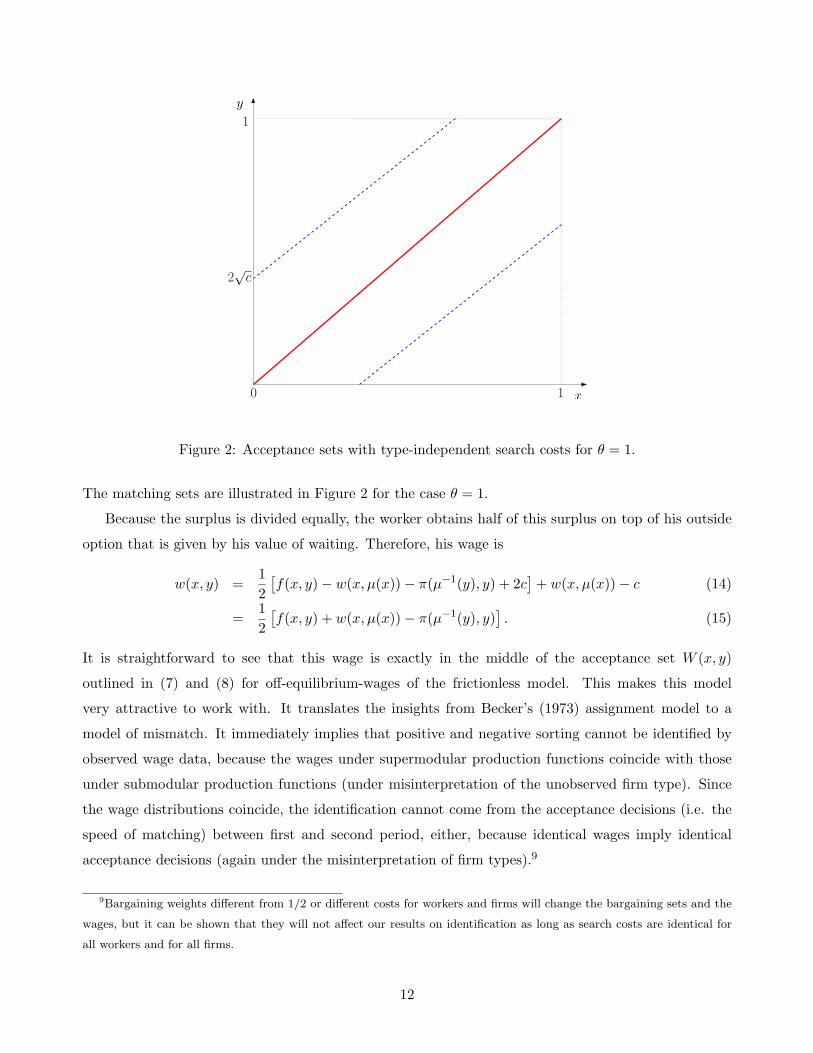
Figure 3: First period wages for under mismatch with a type y = x + k that is k away from the bliss

point. [Graph for x = .5, c = .25, α = θ = 1, h(x) = 0.]

Proposition 3 For every supermodular production function f+ ∈ F+ that induces positive sorting

there is a submodular production function f− ∈ F− that induces exactly the same wages for workers

when we reinterpret firm types as y = 1− y.

Proof. Wages in the second period coincide by Proposition 1. Wages in the first period coincide because

they are in the exact arithmetric middle of the wage set W (., .) which by Proposition (2) coincide under

the re-interpretation.

For our example production technology f+ we get as wages

w(x, y) =α

2(xy)θ +

α

4x2θ − α

4y2θ + h(x).

For some of the results it will be instructive to rewrite the wages as a function of the distance k between

the worker and the firm, which for the special case of θ = 1 becomes particularly tractable:

w(x, x− k) = w(x, x+ k) =α

2x2 − α

4k2 + h(x).

This shows that a worker has a bliss point when matching with a firm with identical type, and

looses quadratically with the distance to the firm. The reason is that a worker who matches with a

13

firm that has too low a type does not produce a lot of output. On the other hand, a worker who wants

to induce a much better firm to match with him has to compensate the firm for not matching with

a more appropriate worker. Therefore it is not necessarily better for a given worker to match with a

higher type firm. In a large region – i.e., whenever the firm is better than the worker – wages fall by

matching with even better firms. Figure 3 illustrates the wage schedule of a worker as a function of the

distance to the firm he matches with, and highlights the fact that the wage falls in firm type in part of

the region. This result holds more generally

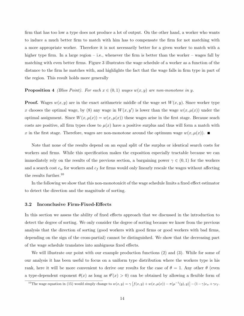
Proposition 4 (Bliss Point). For each x ∈ (0, 1) wages w(x, y) are non-monotone in y.

Proof. Wages w(x, y) are in the exact arithmetric middle of the wage set W (x, y). Since worker type

x chooses the optimal wage, by (8) any wage in W (x, y′) is lower than the wage w(x, µ(x)) under the

optimal assignment. Since W (x, µ(x)) = w(x, µ(x)) these wages arise in the first stage. Because seach

costs are positive, all firm types close to µ(x) have a positive surplus and thus will form a match with

x in the first stage. Therefore, wages are non-monotone around the optimum wage w(x, µ(x)).

Note that none of the results depend on an equal split of the surplus or identical search costs for

workers and firms. While this specification makes the exposition especially tractable because we can

immediately rely on the results of the previous section, a bargaining power γ ∈ (0, 1) for the workers

and a search cost cw for workers and cf for firms would only linearly rescale the wages without affecting

the results further.10

In the following we show that this non-monotonicit of the wage schedule limits a fixed effect estimator

to detect the direction and the magnitude of sorting.

3.2 Inconclusive Firm-Fixed-Effects

In this section we assess the ability of fixed effects approach that we discussed in the introduction to

detect the degree of sorting. We only consider the degree of sorting because we know from the previous

analysis that the direction of sorting (good workers with good firms or good workers with bad firms,

depending on the sign of the cross-partial) cannot be distinguished. We show that the decreasing part

of the wage schedule translates into ambiguous fixed effects.

We will illustrate our point with our example production functions (2) and (3). While for some of

our analysis it has been useful to focus on a uniform type distribution where the workers type is his

rank, here it will be more convenient to derive our results for the case of θ = 1. Any other θ (even

a type-dependent exponent θ(x) as long as θ′(x) > 0) can be obtained by allowing a flexible form of10The wage equation in (15) would simply change to w(x, y) = γ

[f(x, y) + w(x, µ(x)) − π(µ−1(y), y)

]− (1−γ)cw +γcf .

14

the distribution Γ(.) for worker and firm types.11 We can therefore restrict attention to the production

function

f(x, y) = αxy + h(x) + g(y), (16)

where the sign of alpha can be either positive or negative.12 Assume it is positive, so that the exercise

is to detect the strength of sorting and not the sign. It is easy to see from (13) that the acceptance set

a(y) = [y −K, y +K] where K = 2√c/α.

Fixed effect estimation relies on the panel dimension of modern data sets. We assume that the

2-stage hiring process process outlined above repeats T times for each agent.13 We allow the observer

to distinguish between first and second-period wages of the search process of each agent. Since second

stage wages are perfectly aligned, it is not possible to back out worker and firm effects independently.

The first stage does have mismatch and we look at the ability of the firm-fixed effect here. This effect is

the wage that a firm pays its worker net of the average wage that worker’s obtain. We assume that the

panel is long enough such that we can abstract from the stochastic nature of the average wage. That

is, the fixed effect of a firm of type y ∈ [2K, 1− 2K] is14

Ψ(y) =∫ y+K

y−K[w(x, y)− wav(x)] dΓ(x|y). (17)

The term Γ(x|y) = Γ(x)/[Γ(y+K)−Γ(y−K)] reflects the distribution of the worker types conditional

on being willing to match with type y and in the following γ(x|y) will denote its density. The restriction

to y ∈ [2K, 1 − 2K] ensures exactly that there is no boundary problem to consider here, nor in the

following derivation of the workers average wage. The average wage of a worker is

wav(x) =∫ x+K

x−Kw(x, y)dΥ(y|x) = h(x) +

α

2x2 − α

4

∫ K

−Kk2υ(x+ k|x)dk (18)

This term is particularly easy under the uniform distribution, where wav(x) = h(x)+αx2/2−αK2/12.

We are interested if this fixed effect is increasing in the type of the firm. That is, we are interested

whether higher productivity firms on average pay higher wages once we control for the average wage11When x is uniformly distributed, then Γ(x) = x. For any strictly increasing tranformation v(x) [such as v(x) = xθ(x)

with θ′(x) > 0] and production function f(v(x), v(y)) we can without loss of generality specify f(x, y) but change the

distributions to Γ(·) = Γ(v−1(·)) and Υ(·) = Υ(v−1(·)). For this exercise we retain symmetric type distributions.12To caputre (3) the term αx(1 − y) can be split in −αxy and αx, where we can attribute the latter to h(x).13Since the worker’s static problem is identical under negative or positive sorting, the panel dimension does not add to

the identification of the sign of the cross-partial. It does allow for identification of the absolute value of the cross-partial,

which is a measure for the loss from mismatch.14We exclude the types close to the edges of the type space as their matching set is constrained. Analyzing this case is

not difficult, but burdensome in notation as the matching set is a(y) = [max0, y − K, min1, y + K]. Neglecting this

part neglects only a small part of the type space when c and thus K is small.

15

that the workers in this firm are getting. Controlling for the workers’ average wage is a feature of the

fixed effects approach outlined in (1). Without controlling for workers average wage it is trivially true

that under supermodularity higher productivity firms pay higher wages (while under submodularity

lower productivity firms pay higher wages). In the range y ∈ [2K, 1− 2K] we get

Ψ′(y) =∫ y+K

y−K

∂w(x, y)∂y

γ(x|y)dx (19)

+ (w(y +K, y)− wav(y +K)) γ(y +K|y)

− (w(y −K, y)− wav(y −K)) γ(y −K|y).

Call the term in the first line Ψ′1(y) and the terms in the second and third line Ψ′

2(y) so that Ψ′(y) =

Ψ′1(y)+Ψ′

2(y). The first effect Ψ′1(y) accounts for the wage change across those workers with which this

firm type matches. The second effect Ψ′2(y) reflects that the set of workers that match with a firm is

slightly changing when the firm type changes.

We will focus initially on the first effect. The wage change induced by a firm is

∂w(x, y)∂y

=α

2x− α

2y.

That is, the low ability workers x < y loose when the firm gets better, while the workers with relatively

high ability x > y gains when the firm gets better. This happens because in the first case the distance

between the worker and the firm grows and the match becomes less efficient, while in the latter case

the distance shrink closer to the optimal assignment. How does this effect turn out?

For a uniform distribution the positive effect that a slightly better firm type has on the high worker

types that it is willing to employ exactly offsets the negative effect on the lower worker types that it

employs.15 It is easy to see that distributions that lead to more weight on high worker types lend more

weight to the positive aspect, while a distribution that lends more weight to negative worker types leads

to a negative effect:Ψ′

1(y) > 0 if γ′(x|y) > 0 for all y

Ψ′1(y) = 0 if γ′(x|y) = 0 for all y

Ψ′1(y) < 0 if γ′(x|y) < 0 for all y.

(20)

This illustrates that the effect that higher firm types have on those workers they have in common with

lower firm types. It is ambiguous, and could go up or down depending on whether the economy exhibits

relatively more high type workers or vice versa.15For the uniform distribution we have

Ψ′1(y) =

1

2K

∫ y+K

y−K

(α

2x − α

2y)

dx =1

2K

∫ K

−K

(α

2(y + k) − α

2y)

dk = 0.

16

For completeness we consider also the second effect that comes through the changing matching set.

This effect is complicated in general, but becomes tractable when we consider the case where the firm’s

type density is linear. Tor constant υ′(y|x) we obtain in the appendix that16

Ψ′2(y) < 0 if γ′(x|y) > 0 for all y

Ψ′2(y) = 0 if γ′(x|y) = 0 for all y

Ψ′2(y) > 0 if γ′(x|y) < 0 for all y.

(21)

For this case the effects Ψ′1(y) and Ψ′

2(y) run therefore in opposite directions, again reducing the overall

effect even when the distribution is not uniform. It is not difficult to construct type distributions for

which the overall effect is always negative or always positive for all types y ∈ [2K, 1− 2K].

One main conclusion is that the ranking of firms even when we know that we have assortative

matching cannot be backed out from the firm-fixed-effects when the distribution is uniform (at least

for interior types y ∈ [2K, 1 − 2K]). The reason is not that workers are actually sorting randomly.

The matching sets can be arbitrarily small so that workers focus on a very narrow band of firms with

whom they are willing to match. The reason is that the increased wages for some workers are offset by

decreased wages on other (worse) workers.

4 Identifying the Strength of Sorting

We have shown that it is not possible to distinguish negative from positive sorting when only wage

and acceptance data is available (Proposition 3). Moreover, in our environment current fixed effects

estimation not only fails at the direction but also at estimating the strength of sorting. This raises the

question whether anything about the strength of sorting can be identified from the data. In economic

terms this might be more interesting than the direction of sorting (positive or negative) since the welfare

depends on matching the right types, not on who these types are. Identifying some information about

the strength of sorting reveals whether welfare depends to a large degree or a small degree on the right

assignment of workers to firms.

In this section we argue that the strength of the sorting will be identifiable if a worker goes through

this hiring process several times - i.e. if a panel dimension is available. It is possible to determine

how much is gained in terms of welfare from matching agents perfectly. The cross-partial can only

be determined within the bounds of the matching sets, though. For firm-worker-pairs that will not

match this cross-partial cannot be determined. Under parametric forms as in our leading example the16For symmetric distributions Γ(·) = Υ(·) this means that υ′(y|x) = γ′(x|y) = r and therefore Ψ′

2(y) < 0 if r > 0,

Ψ′2(y) = 0 if r = 0 and Ψ′

2(y) > 0 if r < 0.

17

cross-partial can be extended to all matches, which makes it possible to evaluate the overall efficiency

loss between perfect sorting and completely random matching.

Since we cannot identify the productivity of a firm, for this section we will rank firms differently.

If the production function is indeed supermodular, we will learn about the cross-partial of f(x, y). If

the cross-partial is negative, we will learn about the cross-partial of misspecified production function

f(x, y) = f(x, 1 − y) because we will misinterpret bad firms as good firms. Since fxy = |fxy| we will

nevertheless learn about the gain from better sorting.

For the empirical implementation two ingredients will be important. First, we rely on the panel

dimension of available data sets. Again we think that the hiring process outlined above repeats T times,

so that we observe T wages w1i , w

2i , ..., w

ti , ..., w

Ti for worker i and T wages w1

j , w2j , ..., w

tj , ..., w

Tj for

firm j. Identical numbers of draws are not important, it just simplifies the exposition. Second, we restrict

attention to workers in a particular occupation and assume that within this occupation a firm of type

y produces f(x, y) with each worker that it hires. That is, a firm y that has three jobs in a specific

profession such as technicians and hires them at skills x1, x2 and x3 obtains output∑3

i=1 f(xi, y). This

allows us to interpret a multi-worker firm as a firm with a single vacancy that interacts with a sequence

of different workers.17 The identification works along three steps.

First, we will exploit the maximum wage of workers and firms to identify their type. For an agent

k (could be a worker or a firm) we consider the maximum wage

wk = maxt∈1,...,T

wtk

If the panel dimension is long enough this wage is arbitrarily close to the optimal wage. That is, if k

is a worker than this wage is close to his theoretical optimum w(k, µ(k)). For the current exposition

we neglect the finite sample difference and assume that maximum wage in the panel exactly coincides

with the theoretical optimum. We can observe the distribution of these wages across workers. This

yields the cumulative distribution ΩW (w) over the maximum wages across workers. Since good workers

achieve high wages, a worker’s rank can be recovered by the relationship

xk = ΩW (wk).

¿From now on we can refer to workers by their type x and call his maximum wage wx. Alternatively we

could have used the average wage of a worker, and determine his type by the rank in the distribution

of average wages relative to all workers. This might be a more robust approach to the worker’s type

when the panel is finite.17We mention the focus on a particular occuption only because it seems hard to argue that the production function has

such a simple separable form accross occupations, while within an occupation this might be less objectionable.

18

Similarly, we can consider firms. Let ΩF (w) be the cumulative distribution across firms over the

maximum wages paid by those firms. We attribute the following rank to a firm

yk = ΩF (wk).

We can now directly refer to firms by their rank y. This type correctly identifies the firms rank when

we order firms by their eagerness of having a good workers (i.e. by their improvement in output from

increasing the workers type). Again, a more robust ranking might be the ranking of firms by their

average wages. It is important that these are ”raw” wages that are not adjusted for the type of worker.

The reason we do not condition is because we want to identify the firms that are more eager to have

higher workers (rank y under PAM, rank 1− y under NAM) without a concern of identifying whether

the firm is truly more productive.

We can identify for each worker x the lowest firm y that it matches with. We call that firm y(x).

If the panel dimension in the data is long enough, y(x) is arbitrarily close to the lower bound of the

workers acceptance range.

Second, we will exploit the spread between the maximum wage and the minimum wage that workers

accept to identify the waiting costs. Again we assume that the minimum wage

wx = mint∈1,...,T

wtx

of the worker with type x coincides with the theoretical minimum that the worker is willing to accept

in the first period of the search process. The costs of waiting are given by the difference between the

maximum and the minimum wage of a worker18

c = wx − wx,

or we can determine it in aggregate by the average range of wages across workers.

Third, we use the relation between the matching set and the cost of waiting to learn about the

strength of the cross-partial. The loss L(x, y) due to mismatch is the value that is created by pair (x, y)

minus their marginal contribution under perfect sorting

L(x, y) = f(x, y)−∫ x

0fx(x, x)dx−

∫ y

0fy(y, y)dy − f(0, 0). (22)

We derive in the appendix the following more concise expression

L(x, y) = −∫ x

y

∫ x

yfxy(x, y)dxdy (23)

18We have assumed identical costs for all workers. The theory can be extended to type-dependent costs c(x). See the

Discussion Section.

19

This is gives the loss when matching is indeed positive assortative. If matching is negative assortative,

we misidentified a worker type as y = 1− y when y is the true type. Nevertheless the loss can be written

exactly as in (23) for the misidentified production function f(x, y) = f(x, y), and so the cross-partial

fxy(x, y) = −fxy(x, 1− y) can be identify correctly except for the sign.

Workers and firms internalize this in their matching decision. If the lowest trading partner of worker

x is in the interior, i.e. y(x) > 0, then this partner’s type is determined by the indifference condition

that the loss from matching equals the joint cost from waiting, i.e.

−∫ x

y(x)

∫ x

yfxy(x, y)dxdy = −2c. (24)

This is a functional equation that identifies fxy evaluated at (x, y(x)), for all x ∈ [0, 1].

The condition identifies the cross-partial because it compares the noise in the matching sets (x−y(x))

to the noise in the wage data (2c). If the wages vary substantially but matching sets are small, there

must be a large loss in matching by slightly deviating from the optimal type, i.e. the cross-partial must

be large.

Obviously this approach gives an idea about the cross-partial only for some parts of the (x, y) space.

Especially, this does not allow for the inference on the cross-partial for pairs of workers and firms that

do not match. We can extend the analysis to the entire type space if we are willing to make more

stringent parametric assumptions on the cross-partials that we assume to hold on the entire parameter

space. Under our leading example f+ the loss due to miscoordination in abolut terms is given by

|L(x, y)| = |α|2

(xθ − yθ)2.

By (24) we can identify the strength of sorting via equation

|α|(xθ − y(x)θ)2 = 4c

or equivalently

x =(2 (c/|α|)1/2 − y(x)θ

)1/θ

as long as y(x) > 0. Parameters |α| and θ can be identified by the joint behavior of x and y(x). Simple

non-linear regression techniques can asses these parameters if one is willing to attribute the noise in the

process to measurement error. The gain measured in the dollar amount that perfect matching generates

in excess of complete mismatch can then be assessed simply as

G =∫ 1

0

∫ 1

0|L(x, y)|dxdy

=|α|2

∫ 1

0

∫ 1

0(xθ − yθ)2dxdy = |α| θ2

(2θ + 1)(θ + 1)2.

20

Clearly one can also use the computed acceptance bounds (12) to integrate up the loss under the

current mismatch compared to the frictionless optimal assignment, or to compare the current mismatch

to complete randomness.

5 Discussion and Extensions

In this paper we pursue two goals. First, we use the most well-known model of sorting by Becker (1973)

to gain insights into the wage setting process. We extend the model in the smallest possible way to

allow for mismatch while retaining the basic idea underlying the assortative matching model. This

allows us to provide analytical expressions for the mismatched wages in the model, to characterize their

bliss point property, and to provide an explicit version of a fixed effects method used in the empirical

literature. We show that the latter is neither well-suited to identify the sign nor the strength of sorting.

Identification of the direction of sorting is in general impossible because firms pay wages based on the

gain they have from employing a higher worker, not because they themselves are productive. Even

under positive sorting the fixed effects approach is not able to identify the strength of sorting because

wages are non-monotone in firm type. This non-monotonicity is at odds with the basic fixed-effects

idea, and we show that the net effect may be zero.

Second, we propose to abandon the attempt to identify from wage data the sign of sorting. The

mere fact that wages are determined mainly by the need for having a better worker (which is based on

the cross-partial and not the first derivatives) makes such identification difficult. Under submodularity

it is the low productivity firms that especially need good workers to increase their (in terms of levels)

meager profits, while under submodularity it is the productive firms that need more productive workers

most. In both cases the firms that need the productive workers most have an incentive to pay high

wages, which makes identification without profit (per job) data difficult. Yet in economic terms the

sign of sorting may be less important than the gain that is achieved by sorting workers into the “right”

job. We show that some information about this gain can be identified from wage data. We propose

a specific method of backing out this strength locally around the equilibrium path. The identification

comes from determining some notion of the size of the set of firms with which a worker matches. If a

worker is only willing to match with a small fraction of firms, for a given level of frictions (which we

can identify from the data) the complementarities must be large. Similarly, when a worker is willing to

match with many firm types the complementarities must be weak. This gives a well-defined notion of

the dollar-value of the gain from sorting in the market.

Our method may well not be the only one that identifies the strength of sorting. Since existing

attempts have mainly considered the sign of sorting, this area is not well-developed. We believe that

21

other methods that compare the noise in the accepted matches of a worker (i.e. the range of the type

space or the range of wages) with the total noise in the market as a whole are promising in shedding light

on this issue. Similarly, one can look at the problem from the firm side. When within-firm variation

of worker types (or their salaries – depending on the model) is low relative to the overall variation in

the data, for given level of frictions complementarities must be large for agents to focus on a narrow

band of matches. For example, Lopes de Melo (2008) considers the within-firm correlation of wages

as a measure. Comparisons with the variation overall might capture something about the strength

of sorting. Evaluating the strength of sorting this way is important in order to assess the welfare-

consequences of matching agents better. The main difficulty is to distinguish the cause of the relative

noise levels. It could be that frictions are high and therefore workers accept nearly all matches, or

complementarities are low. The challenge is to propose procedures that separate the source of frictions

from the complementarity, and the procedure in the previous section presents one approach to do this.

We now briefly discuss some of the other issues that may be of importance in identifying sorting.

On-the-job-search. On-the-Job-Search (OJS) is a likely candidate for identifying sorting using equi-

librium mismatch (see also Bagger and Lentz (2008) and Lopes de Melo (2008)). As long as a job is

scarce, matched pairs face a trade-off between matching early and waiting.19 Like in our models with

friction, this induces a trade-off between accepting some degree of mismatch and waiting. With OJS,

this happens simultaneously.

Using Data on Profits: the Attribution Problem. One obvious observation is that with data on

profits we can identify both the strength and the sign of sorting. And while there are good data on

firm profits, there are no data on job profits. In multi-worker firms, we need to attribute the share of

each worker’s contribution to the overall firm profits. Even in the simplest economy we need to decide

what the contribution of very different individuals (CEO, secretary and janitor) is to the firm profit.

Since this decomposition seems difficult across occupations, we propose to focus on the economically

important and manageable problem of the identifying the strength of sorting.

Being aware of the shortcomings of the wage data in fixed effects estimates, Mendes, van den Berg,

and Lindeboom (2007) use productivity data instead. They choose average firm-specific productivity to

attribute output from the firm to an individual worker. They find that average firm-specific productivity

and worker skill exhibit strong positive sorting.

More General Technologies. Above, we have shown that the strength of the sorting can be identified,

but not the sign. This suggests that our analysis extends to an even broader class of preferences.19In Bagger and Lentz (2008) jobs are not scarce since firms can open as many jobs as they want. The sorting effect in

their model derives from differences in the intensity by which workers search for a new job.

22

Suppose output is maximized when “similar” agents match, then there is no ranking of better jobs, but

we can still identify how strong the complementarity is between workers with our approach. Observe

that this does include more realistic cases of production technologies where types are multi-dimensional.

All the information that we use to identify the sorting effect is embedded in the wages, thus giving us

a monetary value (and therefore one-dimensional order) of sorting.

Type-Dependent Search Costs. We analyzed a model of matching that replicates the payoffs of the

model by Becker (1973). While in Becker sorting is perfect and matches lie only on the diagonal of the

type distribution, we extend his setting to allow for matches also off that diagonal, while retaining the

payoffs that Becker’s competitive model predicts for such matches by following the basic methodology

of Atakan (2006).

The introduction of waiting costs can be done in ways that deliver wages that do not coincide with

those predicted in Becker’s theory. For example, introducing waiting costs through time discounting

with factor β ∈ (0, 1) along a methodology similar to Shimer and Smith (2000) leads to different payoffs.

The reason is that waiting costs are now different for different types, with higher types suffering a higher

loss when they don’t trade immediately. This allows workers to gain from trading with higher types.

While this potentially makes identification possible (in contrast to Section 3), the variability that is

introduced is small when discounting is large because wages are still mainly determined by the need

of hiring better workers. More severely, even under differential waiting costs in the current empirical

approach via fixed effects it is not guaranteed that higher productivity firms on average pay higher

wages after controlling for worker types (similar to Section 4).

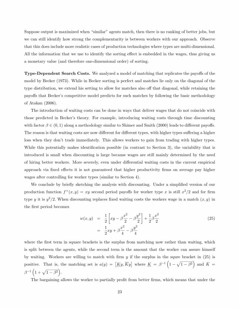
We conclude by briefly sketching the analysis with discounting. Under a simplified version of our

production function f+(x, y) = xy second period payoffs for worker type x is still x2/2 and for firm

type y it is y2/2. When discounting replaces fixed waiting costs the workers wage in a match (x, y) in

the first period becomes

w(x, y) =12

[xy − β

x2

2− β

y2

2

]+

12βx2

2(25)

=12xy + β

x2

4− β

y2

4

where the first term in square brackets is the surplus from matching now rather than waiting, which

is split between the agents, while the second term is the amount that the worker can assure himself

by waiting. Workers are willing to match with firm y if the surplus in the squre bracket in (25) is

positive. That is, the matching set is a(y) =[Ky,Ky

]where K = β−1

(1−

√1− β2

)and K =

β−1(1 +

√1− β2

).

The bargaining allows the worker to partially profit from better firms, which means that under the

23

submodular specification f−(x, y) = (1− y)x+ y the wage will be as in (25) when we replace y by its

transform y = 1− y, plus an added term 12(1− β)(1− y). This added term is small when β is close to

one relative to the other terms in the wage equation, and therefore potentially difficult to detect with

statistical significance when job finding rates are high (i.e., when the associated time difference between

first and second period is low). Nevertheless, the term is not coincidental in the sense that identical

second period wages will require differences in first period wages induced by bargaining, and sufficient

data quantities might allow it to be backed out in a structural estimation.20

The current fixed effect estimators are still not well suited to detect this effect. While now workers

benefit in the bargaining stage from higher types, this effect is linear, while the opportunity cost

of occupying the “wrong” job is increasing more than linearly whenever the production function is

supermodular. This is reflected by the quadratic negative term in the wage equation and is also reflected

in the lower bound of the acceptance set a(y). The reason why very low workers are not willing to match

with this firm is that their wage would be too bad because they would have to compensate the firm for

forgoing very profitable production opportunities in the future.

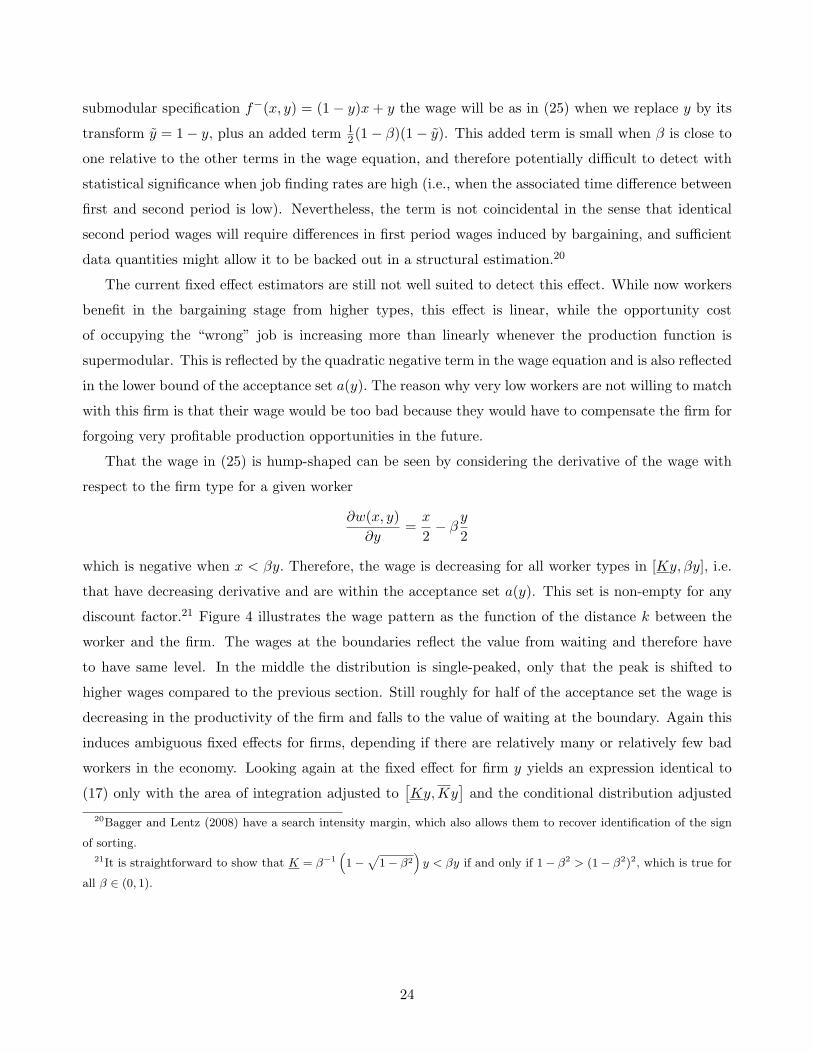
That the wage in (25) is hump-shaped can be seen by considering the derivative of the wage with

respect to the firm type for a given worker

∂w(x, y)∂y

=x

2− β

y

2

which is negative when x < βy. Therefore, the wage is decreasing for all worker types in [Ky, βy], i.e.

that have decreasing derivative and are within the acceptance set a(y). This set is non-empty for any

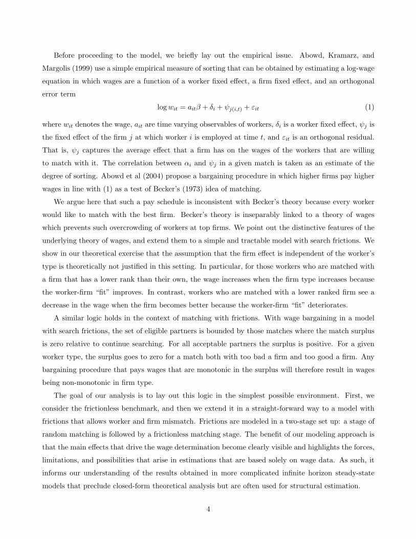
discount factor.21 Figure 4 illustrates the wage pattern as the function of the distance k between the

worker and the firm. The wages at the boundaries reflect the value from waiting and therefore have

to have same level. In the middle the distribution is single-peaked, only that the peak is shifted to

higher wages compared to the previous section. Still roughly for half of the acceptance set the wage is

decreasing in the productivity of the firm and falls to the value of waiting at the boundary. Again this

induces ambiguous fixed effects for firms, depending if there are relatively many or relatively few bad

workers in the economy. Looking again at the fixed effect for firm y yields an expression identical to

(17) only with the area of integration adjusted to[Ky,Ky

]and the conditional distribution adjusted

20Bagger and Lentz (2008) have a search intensity margin, which also allows them to recover identification of the sign

of sorting.21It is straightforward to show that K = β−1

(1 −

√1 − β2

)y < βy if and only if 1 − β2 > (1 − β2)2, which is true for

all β ∈ (0, 1).

24

Figure 4: First period wages for under mismatch with a type that is k away from the bliss point. [Graph

for x = .5, β = .98]

to Γ(x|y) = Γ(x)/[Γ(Ky)− Γ(Ky)]. Analogous to (19) this leads to a change in the fixed effect of22

Ψ′(y) =∫ Ky

Ky

(12x− 1

2βy

)γ(x|y)dx

+K

(βK

2y2

2− wav(Ky)

)γ(Ky|y)

−K(βK2y2

2− wav(Ky)

)γ(Ky|y).

While this fixed effect is harder to analyze than expression (19) for type-independent search costs, it is

still easy to see that this expression is not in general positive. The first line is negative if γ is sufficiently

decreasing, because then γ(x|y) is sufficiently decreasing and the type space gives more weight to low

worker types. On average the workers suffer from an improvement in the firm quality because the firm

moves further from the bliss point of the low worker types which are more predominant. Also, the third

line is larger than the second when γ(x|y) is sufficiently decreasing. Both effects together clearly induce

an effect in which better firms have lower fixed effects because most workers in the economy have a type

lower then them. Again we believe that an approach based on the bounds of the acceptance set relative

to the entire type space similar to Section 4 will be useful in considering the strength of sorting..

22The second line in the following expression only arises for Ky < 1, otherwise the upper bound is 1 and is not affected

by a change in y.

25

6 Concluding Remarks

We argue that identifying the sign of sorting from wage data alone is difficult, if not impossible. The

main reason is that the wages reflect at least in part the marginal contribution to the value that the

firm generates, and it can be either the more productive or the less productive firms that have a higher

marginal benefit from employing a better worker. The empirical question whether or not there is

evidence of sorting remains to be answered. In many settings we expect more able workers to have a

higher marginal contribution to more productive firms, but in some industries more productive firms

have invested in automatization that allows workers with lower skills to perform the high productivity

jobs (e.g. retail trade). We argue that it is possible to identify the strength of sorting, though the

commonly used fixed effect methods are not suitable for the task. With estimates of the strength of

sorting in hand, the objective is to be able to assess the efficiency implications.

26

7 Appendix

Derivation of (21): Observe that both w(y +K, y) and w(y −K, y) are wages for workers that are

exactly indifferent between matching now and not matching. This indifference implies w(y + K, y) =

h(y+K)+ α(y+K)2

2 − c and w(y−K, y) = h(y−K)+ α(y−K)2

2 − c. Since the average wage than a worker

gets when matching in the first stage is better than not matching, the difference between these wages

and the average wage is negative. Using these expressions and the term for the average wage in (18)

we obtain

Ψ′2(y) = −

[c− α

4

∫ K

−Kk2υ(y +K + k|y +K)dk

]γ(y +K|y) (26)

+[c− α

4

∫ K

−Kk2υ(y −K + k|y −K)dk

]γ(y −K|y).

This effect depends on y only through the effect on the distribution. Therefore, again this effect is zero

under a uniform distribution. For other distributions the effect is ambiguous because it relies on the

density at the endpoints as well as on the integral over the density. In the special case where υ′(y|x) = r

is constant the density is linear, and so are the conditional densities. In such a case symmetry around

zero of k2 ensures that −14

∫K−K k2υ(Y + k|Y )dk is independent of Y and the terms in square brackets

are identical, which directly leads to the inequalities in (21).

Derivation of (23): Equation (23) can be expanded to

L(x, y) =∫ y

0fy(x, y)dy + f(x, 0)−

∫ x

0fx(x, x)dx−

∫ y

0fy(y, y)dy − f(0, 0)

=∫ y

0

∫ x

0fxy(x, y)dxdy +

∫ y

0fy(0, y)dy + f(x, 0)

−∫ x

0

∫ x

0fxy(x, y)dydx−

∫ x

0fx(x, 0)dx−

∫ y

0

∫ y

0fxy(x, y)dxdy −

∫ y

0fy(y, 0)dy − f(0, 0)

=∫ y

0

∫ x

yfxy(x, y)dxdy −

∫ x

0

∫ x

0fxy(x, y)dydx

Let x ≥ y. (The derivation under the opposite follows analogous steps.) Then we have

L(x, y) =∫ y

0

∫ x

yfxy(x, y)dxdy −

∫ x

0

∫ x

0fxy(x, y)dydx (27)

Note that∫ x0

∫ x0 fxy(x, y)dydx integrates for each x over all y ≤ x. Similarly, one can for each y integrate

over all y ≥ x. That is ∫ x

0

∫ x

0fxy(x, y)dydx =

∫ x

0

∫ x

yfxy(x, y)dxdy.

Therefore, (27) becomes

L(x, y) =∫ y

0

∫ x

yfxy(x, y)dxdy −

∫ x

0

∫ x

yfxy(x, y)dxdy = −

∫ x

y

∫ x

yfxy(x, y)dxdy.

27

References

[1] Abowd, J.M., F. Kramarz, and D. N. Margolis, “High Wage Workers and High Wage

Firms,”Econometrica 67, 1999, 251 - 333.

[2] Abowd, J.M., F. Kramarz, P. Lengermann, and S. Perez-Duarte, “Are Good Workers

Employed at Good Firms? A Test of a Simple Assortative Matching Model for France and the

United States.” Cornell mimeo 2004.

[3] Acemoglu, Daron, and Robert Shimer, ”Efficient Unemployment Insurance,” Journal of

Political Economy 107, 1999a, 893-928.

[4] Atakan, Alp E., “Assortative Matching with Explicit Search Costs”, Econometrica 74(3), 2006,

667–680.

[5] Bagger, Jesper, and Rasmus Lentz, “An Equilibrium Model of Wage Dispersion and Sort-

ing,”U Wisconsin mimeo 2008.

[6] Becker, Gary S., ”A Theory of Marriage: Part I”, Journal of Political Economy 81(4), 1973,

813-46.

[7] Eeckhout, Jan and Philipp Kircher, “Sorting and Decentralized Price Competition”, UPenn

mimeo, 2008.

[8] Gautier, Pieter A. and Coen N. Teulings, “How Large are Search Frictions”, Journal of the

European Economic Association, 4(6), 2006, 1193-1225.

[9] Lise, Jeremy, Costas Meghir, and Jean-Marc Robin, “Matching, Sorting and Wages ”,

UCL mimeo, 2008.

[10] Lopes de Melo, Rafael, “Sorting in the Labor Market: Theory and Measurement”, Yale mimeo,

2008.

[11] Mendes, Rute, Gerard van den Berg, Maarten Lindeboom, “An empirical assessment of

assortative matching in the labor market”, Uppsala mimeo 2007.

[12] Sattinger, Michael, “Comparative Advantage and the Distributions of Earnings and Abilities”,

Econometrica 43(3), 1975, 455–468.

[13] Shapley, Lloyd S. and Martin Shubik, “The Assignment Game I: The Core”, International

Journal of Game Theory 1(1), 1971, 111-130.

28

[14] Shimer, Robert, and Lones Smith, “Assortative Matching and Search,” Econometrica 68,

2000, 343–369.

29