phytoplankton scales of variability in the california

Phytoplankton scales of variability in the California Current System:

2. Latitudinal variability

Stephanie A. Henson1 and Andrew C. Thomas1

Received 30 November 2006; revised 23 March 2007; accepted 24 April 2007; published 14 July 2007.

[1] The California Current System encompasses a southward flowing current which isperturbed by ubiquitous mesoscale variability. The extent to which latitudinal patterns ofphysical variability are reflected in the distribution of biological parameters is poorlyknown. To investigate the latitudinal distribution of chlorophyll variance, a waveletanalysis is applied to nearly 9 years (October 1997 to July 2006) of 1-km-resolutionSea-viewing Wide Field-of-view Sensor (SeaWiFS) chlorophyll concentration data at5-day resolution. Peaks in the latitudinal distribution of chlorophyll variance coincide withfeatures of the coastal topography. Maxima in variance are located offshore of VancouverIsland and downstream of Heceta Bank, Cape Blanco, Point Arena, and possibly PointConception. An analysis of dominant wavelengths in the chlorophyll data reveals atransfer of energy into smaller scales is generated in the vicinity of the coastal capes. Thelatitudinal distribution of variance in sea level anomaly corresponds closely to thechlorophyll variance in the nearshore region (<100 km offshore), suggesting that the sameprocesses determine the distribution of both. Farther offshore, there is no correspondencebetween latitudinal patterns of sea level anomaly and chlorophyll variance. This likelyrepresents a transition from physical to biological control of the phytoplanktondistribution.

Citation: Henson, S. A., and A. C. Thomas (2007), Phytoplankton scales of variability in the California Current System: 2.

Latitudinal variability, J. Geophys. Res., 112, C07018, doi:10.1029/2006JC004040.

1. Introduction

[2] The California Current System (CCS) is an easternboundary flow extending from the bifurcation of the WestWind Drift at �50�N to Baja California. Seasonally varyingequatorward winds result in vigorous coastal upwelling anda predominantly southward surface flow [Hickey, 1998].The equatorward current develops meanders, filaments andeddies, evident in satellite imagery of sea surface tempera-ture (SST) and phytoplankton pigment [e.g., Traganza etal., 1980; Ikeda et al., 1984a, 1984b; Ramp et al., 1991;Abbott and Barksdale, 1991]. The structures observed inSST and Coastal Zone Color Scanner (CZCS) data corre-spond closely, implying that physical processes are impor-tant to phytoplankton distribution in this region [Abbott andZion, 1985; Denman and Abbott, 1994]. In the CCS therole of mesoscale variability in several biological processeshas been demonstrated, for example, delivery of nutrients[Chavez et al., 1991], offshore transport of phytoplankton[Washburn et al., 1991] and zooplankton community com-position and distribution [Mackas et al., 1991].[3] The location of persistent meanders and filaments in

the southward flowing jet are often associated with thecoastal topography. From Washington to Point Conception(�34�N–48�N) the coastline is aligned almost north-south

but several capes protrude from the coast, deflecting thejet offshore. The flow-topography interaction results inincreased mesoscale variability in the vicinity of the capes[e.g., Ikeda and Emery, 1984a; Haidvogel et al., 1991;Batteen et al., 2003; Marchesiello et al., 2003; Castelaoand Barth, 2005] and enhanced biomass in the lee of thecapes has also been observed [Barth et al., 2005; Huyer etal., 2005].[4] Satellite data are well suited to the task of assessing

phytoplankton variability, as it provides repeated, synopticimagery over large spatial and temporal scales. To extractthe dominant modes of variability we employ the method ofwavelet analysis, which decomposes a signal into time-frequency, or distance-wavelength, space. In a companionpaper [Henson and Thomas, 2007] (hereinafter HT07) adetailed description of the wavelet transform is given, with afocus on interpreting the results of an analysis. HT07quantifies the dominant temporal scales of phytoplanktonvariability in SeaWiFS chlorophyll concentration (chl a)data as a function of cross-shelf distance using latitudinalmeans of the entire study region and identifies their seasonaland interannual variability. Maximum variance in chloro-phyll was found to have a period of �100–200 days. Thetiming of peak variance varied seasonally with cross-shelfdistance, with maxima in spring/summer close to shore andin autumn/winter offshore, consistent with the seasonaloffshore migration of the coastal jet. Substantial interannualvariability in the magnitude of chlorophyll variance wasalso observed and found to be strongly out of phase with the

JOURNAL OF GEOPHYSICAL RESEARCH, VOL. 112, C07018, doi:10.1029/2006JC004040, 2007ClickHere

for

FullArticle

1School of Marine Sciences, University of Maine, Orono, Maine, USA.

Copyright 2007 by the American Geophysical Union.0148-0227/07/2006JC004040$09.00

C07018 1 of 11

http://dx.doi.org/10.1029/2006JC004040

Pacific Decadal Oscillation index. In this paper we applywavelet analysis to the same SeaWiFS chl a data set as inHT07 to assess the latitudinal distribution of chlorophyllvariance.

2. Data

[5] Daily SeaWiFS chlorophyll a (chl a) concentrationdata at 1 km resolution were downloaded from the NASAOcean Color Browser (http://oceancolor.gsfc.nasa.gov/). Alllevel 2 MLAC files (v5.1 reprocessing) from 2 October1997 to 31 July 2006 in the boundaries 34�N–50�N,130�W–118�W (Figure 1) were downloaded. Individualpasses were remapped to a cylindrical projection andmultiple passes on a calendar day were composited. Onaverage �20% of the data were missing owing to cloudi-ness, and therefore daily images were then composited into5-day means to reduce gaps. Any gaps shorter than three

time steps (i.e., 15 days) in length were filled by linearinterpolation in time. Remaining gaps were filled with amean value, calculated for that pixel and 5-day period fromall valid data in other years. The climatological meanseasonal cycle, calculated at each pixel, was removed fromthe data prior to performing wavelet analysis. The resultingtime series were subsampled as transects parallel to the coastat distances 20, 50, 100 and 200 km offshore (Figure 1).[6] Multimission (JASON and TOPEX/POSEIDON)

gridded SLA data at 7-day, 0.25� resolution from October1997 to July 2006 were obtained from http://www.aviso.oceanobs.com. The climatological seasonal cycle wasremoved from the data prior to analysis. Transects parallelto the coast were extracted at the same locations as the chl adata. In the transect closest to shore, data are absent between41�N and 42�N owing to land detection errors in the AVISOdata set.[7] We briefly illustrate the wavelet analysis method

using an example time series of SeaWiFS chl a data at43.8�N, 124.8�W. Further details of the method used aregiven by HT07 and formal mathematical descriptions byMorlet [1983] or Daubechies [1992]. A Morlet-6 wavelettransform was applied to the time series (Figure 2a). Theresulting local wavelet power spectrum (Figure 2b)describes the relative amplitude of features at a particularfrequency and time. The contours represent wavelet powerand can be interpreted as a ‘map’ of the time variability ofdominant frequencies. The unit of wavelet power is theoriginal data unit squared, i.e., the variance (in the case ofchl a this is (mg m�3)2). Thick solid lines denote the 95%confidence level, assuming a white-noise background spec-trum [Torrence and Compo, 1998]. Errors increase at theedges of the wavelet spectrum owing to the finite length ofthe time series, and data below the cone of influence (thinsolid line in Figure 2b) should be regarded with caution. Inthis example, the largest peak in wavelet power occurs in2002 with dominant periods of �70–150 days. Smallerpeaks occur in 1998, 2003, 2004 and 2005 with periods of�80–120 days, and relatively weak wavelet power isevident only at periods greater than �200 days in 1999and 2000.[8] The information contained in the local wavelet spec-

trum can be summarized by the global wavelet powerspectrum (GWPS; Figure 2c) and scale-averaged time series(Figure 2d). The GWPS is the time-averaged wavelet powerat each period and in this example has a peak at periods�100 days (Figure 2c). The scale-averaged time series is themean variance contained in a certain period band. Averag-ing over the period band 80–120 days (Figure 2d) indicatesthat maximum variance occurs throughout 2002 and in2005. In 1999 and 2000 variance in this period band isbelow the 95% confidence level.

3. Results

[9] At each pixel along a transect (1 km spacing) awavelet analysis was performed on the time series of data.The resulting local wavelet power spectra were scale-averaged over a period band of �100�200 days (as inFigure 2d), the range of periods in which peak chl a isgenerally observed (HT07). The scale-averaged time seriesfor each transect (20, 50, 100 and 200 km offshore) are then

Figure 1. Map of the study region showing bathymetriccontours at 50, 200, and 500 m depth. The dashed lineshows the location of the 100-km offshore transect. Blackdot marks position of example time series in Figure 2a.Locations mentioned in the text are labeled.

C07018 HENSON AND THOMAS: CCS PHYTOPLANKTON VARIABILITY, 2

2 of 11

C07018

combined into a two-dimensional view of the temporal andspatial variability of chl a variance in this particular periodband (contour plots in Figures 3a–3d), known as ‘powerHovmoller’ plots [Torrence and Compo, 1998]. Thickblack lines enclose regions with >95% confidence. In thispaper our focus is on the latitudinal distribution of chl avariance. The interannual variability is discussed in HT07.Line plots in Figures 3e–3h show the latitudinal distribu-tion of the time averaged variance in chl a at periods of100–200 days.[10] At each distance offshore, maximum variance occurs

between 46�N–50�N (in the vicinity of Vancouver Island)and 36�N–38�N (south of Point Arena). High varianceoccurs consistently every year north of �48�N, but is morepatchy farther south. At 20 km offshore, maxima in chl avariance occur at 46�N–50�N and 36�N–39�N (Figure 3a).Peaks in variance in the north occur consistently in all years(although in 2000 variance is particularly weak). The timemean variance (Figure 3e) has peaks at 46�N–50�N, 44�N

(near Heceta Bank), 43�N (in the vicinity of Cape Blanco),40�N–41.5�N (near Cape Mendocino), 36�N–39�N and35�N (north of Point Conception). At a distance of 50 kmoffshore, the time mean variance (Figure 3f) has broadpeaks at 46�N–50�N, 40�N–42�N and 36�N–38�N. Alocalized maximum occurs at 44�N. At 100 km offshore,the time mean variance (Figure 3g) has a broad peakbetween 47�N and 50�N and smaller maxima at 45�N,44�N and 43�N. Another broad peak occurs at 40�N�42�Nand 36�N–38�N. At 200 km offshore, largest peaks in thetime mean chl a variance (Figure 3h) occur at 36�N–38�Nand 48�N. Smaller peaks are regularly spaced (�150 kmapart) between 38�N and 47�N.[11] A clear structure is observed in the latitudinal distri-

bution of chl a variance. However, the plots in Figure 3 areonly for the period band 100–200 days. It is fair to askwhether locations with low chl a variance in the 100- to200-day band are characterized by low variance in general,or whether peak wavelet power is shifted into different

Figure 2. (a) Time series of SeaWiFS chl a anomalies at 43.8�N, 124.8�W. (b) Local wavelet powerspectrum of the time series. High values of wavelet power indicate frequencies and times at which chl avariance is high. Thick black line is the 95% confidence level. Thin line is the cone of influence, belowwhich edge effects become important. The y axis has been converted from wavelet scale, a, to frequency.For the Morlet-6 wavelet, frequency = 1.03a [Torrence and Compo, 1998]. The smallest scale resolved isat the Nyquist frequency (�10 days). (c) Global wavelet power spectrum, i.e., the temporal mean waveletpower at each period. Dashed line is the 95% confidence level. (d) Scale-averaged time series for theperiod band 80–120 days. Wavelet power has been normalized by N/2s2 (where N is the number of datapoints and s2 is its variance). Dashed line is the 95% confidence level.


3 of 11

C07018

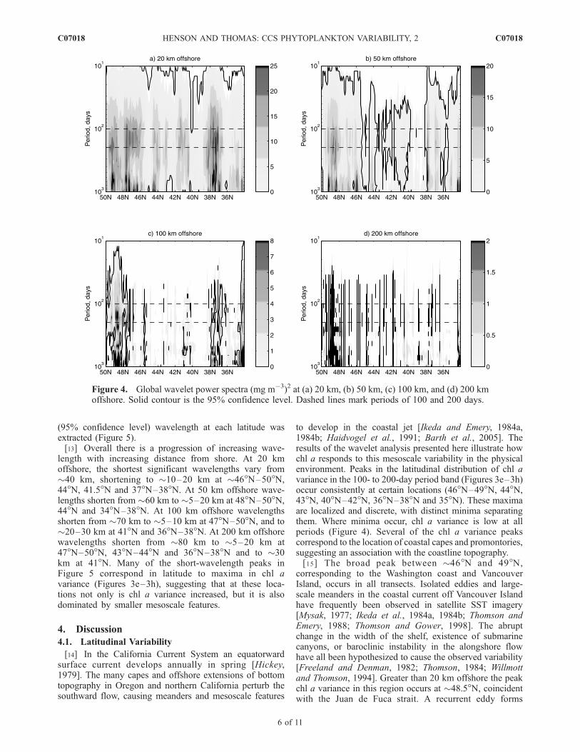
periods and therefore not represented in Figure 3. Thelatitudinal distribution of wavelet power in multiple periodbands can be assessed using the global wavelet powerspectrum (as in Figure 2c). At each point in a transect thewavelet transform is applied to the time series of chl a data.The resulting global spectra (and 95% confidence level) arecontoured as a function of latitude in Figure 4. Note thatalthough a particular period or location may not contain any

statistically significant wavelet power globally (i.e., aver-aged over all time), it may still have significant local power(i.e., at a particular point in time), and vice versa. InFigure 4 vertically oriented structure indicates coherenceacross period bands. At 20 km offshore, wavelet poweroccurs at a wide range of periods at most latitudes. Drops inpower occur at all periods at �45�N, 43�N, 39�N and 36�N.At 50 km offshore statistically significant wavelet power

Figure 3. Power Hovmoller plots for scale-averaged (period band �100–200 days) chl a waveletpower for transects taken (a) 20 km offshore, (b) 50 km offshore, (c) 100 km offshore, and (d) 200 kmoffshore. Thick black line indicates the 95% confidence level. Time-averaged power spectra for periodband �100–200 days as a function of latitude for transects (e) 20 km offshore, (f) 50 km offshore,(g) 100 km offshore, and (h) 200 km offshore. Maps of study region show bathymetric contours at50, 200, and 500 m depth. Locations mentioned in text are labeled.


4 of 11

C07018

occurs at a large range of periods only between �46�N–50�N and 34�N–38�N. Statistically significant poweroccurs only at periods �50–400 days between �40�Nand 43�N. At 45�N and 38�N–40�N there is very littlestatistically significant wavelet power at any period. Onehundred kilometers offshore high, statistically significantwavelet power occurs from �20 to 400 days at �48�N–50�N and 34�N. Apart from these two areas statisticallysignificant wavelet power is scarce, with only small patches,principally �37�N–38�N. By 200 km offshore statisticallysignificant wavelet power is very sparse with the onlyspatially coherent area occurring �48�N–50�N. At eachdistance from shore, Figure 4 demonstrates that maxima andminima in variance are strongly coherent across period

bands at each latitude. At locations where chl a varianceis low in the 100- to 200-day period band, wavelet power isgenerally low at all periods, and is not simply shifted intodifferent periods.[12] To investigate the latitudinal distribution of the

wavelengths (rather than periods) of chl a variance weemployed a spatial wavelet analysis (all results so far havebeen from a temporal analysis). The resulting waveletpower spectra are a function of distance and wavelength(rather than time and period). For each location 20, 50, 100and 200 km offshore a wavelet analysis was performed on atime-averaged transect of chl a. From the resulting localwavelet power spectra, the shortest statistically significant

Figure 3. (continued)


5 of 11

C07018

(95% confidence level) wavelength at each latitude wasextracted (Figure 5).[13] Overall there is a progression of increasing wave-

length with increasing distance from shore. At 20 kmoffshore, the shortest significant wavelengths vary from�40 km, shortening to �10–20 km at �46�N–50�N,44�N, 41.5�N and 37�N–38�N. At 50 km offshore wave-lengths shorten from �60 km to �5–20 km at 48�N–50�N,44�N and 34�N–38�N. At 100 km offshore wavelengthsshorten from �70 km to �5–10 km at 47�N–50�N, and to�20–30 km at 41�N and 36�N–38�N. At 200 km offshorewavelengths shorten from �80 km to �5–20 km at47�N–50�N, 43�N–44�N and 36�N–38�N and to �30km at 41�N. Many of the short-wavelength peaks inFigure 5 correspond in latitude to maxima in chl avariance (Figures 3e–3h), suggesting that at these loca-tions not only is chl a variance increased, but it is alsodominated by smaller mesoscale features.

4. Discussion

4.1. Latitudinal Variability

[14] In the California Current System an equatorwardsurface current develops annually in spring [Hickey,1979]. The many capes and offshore extensions of bottomtopography in Oregon and northern California perturb thesouthward flow, causing meanders and mesoscale features

to develop in the coastal jet [Ikeda and Emery, 1984a,1984b; Haidvogel et al., 1991; Barth et al., 2005]. Theresults of the wavelet analysis presented here illustrate howchl a responds to this mesoscale variability in the physicalenvironment. Peaks in the latitudinal distribution of chl avariance in the 100- to 200-day period band (Figures 3e–3h)occur consistently at certain locations (46�N–49�N, 44�N,43�N, 40�N–42�N, 36�N–38�N and 35�N). These maximaare localized and discrete, with distinct minima separatingthem. Where minima occur, chl a variance is low at allperiods (Figure 4). Several of the chl a variance peakscorrespond to the location of coastal capes and promontories,suggesting an association with the coastline topography.[15] The broad peak between �46�N and 49�N,

corresponding to the Washington coast and VancouverIsland, occurs in all transects. Isolated eddies and large-scale meanders in the coastal current off Vancouver Islandhave frequently been observed in satellite SST imagery[Mysak, 1977; Ikeda et al., 1984a, 1984b; Thomson andEmery, 1988; Thomson and Gower, 1998]. The abruptchange in the width of the shelf, existence of submarinecanyons, or baroclinic instability in the alongshore flowhave all been hypothesized to cause the observed variability[Freeland and Denman, 1982; Thomson, 1984; Willmottand Thomson, 1994]. Greater than 20 km offshore the peakchl a variance in this region occurs at �48.5�N, coincidentwith the Juan de Fuca strait. A recurrent eddy forms

Figure 4. Global wavelet power spectra (mg m�3)2 at (a) 20 km, (b) 50 km, (c) 100 km, and (d) 200 kmoffshore. Solid contour is the 95% confidence level. Dashed lines mark periods of 100 and 200 days.


6 of 11

C07018

annually in summer at the mouth of the strait. Its influence,reflected in SST, density and velocity structure, extends>150 km offshore [Freeland andDenman, 1982;MacFadyenet al., 2005]. These processes which contribute variance tothe physical system appear to be reflected in enhancedbiological variance too.[16] A large submarine bank, Heceta Bank, extends

�50 km offshore between 43.8�N and 44.6�N. The bankdisrupts the alongshore flow of the coastal jet, increasing itsoffshore excursion [Castelao and Barth, 2005]. A low-velocity zone is located inshore of the bank, resulting inretention of water and accumulation of biomass, bothzooplankton and phytoplankton [Barth et al., 2005]. Wefind a narrow peak in chl a variance at �44�N in the twonearshore transects (20 and 50 km offshore). At 100 kmoffshore the peak is much smaller and not well separatedfrom neighboring peaks, and at 200 km offshore the clearpeak has vanished altogether. Chl a variance is increasednearshore on the downstream edge of Heceta Bank, but notoffshore of the 200-m isobath (which lies �70 km offshorehere).[17] Cape Blanco (�43�N) separates a region to the

north where the coastal jet lies close to the shore, from a

region to the south where the jet meanders well offshore ofthe shelf [Barth et al., 2000]. The flow-topography inter-action and locally intensified wind speed and wind stresscurl downwind of Cape Blanco [Samelson et al., 2002;Perlin et al., 2004] greatly increases the mesoscale activitydownstream (i.e., south) of the Cape, where more convo-luted fronts are observed in SST imagery [Castelao andBarth, 2005]. At the Cape itself (i.e., at 43�N) chl avariance is at a minimum, but a broad maximum occursbetween �40�N and 42�N, up to �100 km offshore(Figures 3e–3h). This is consistent with the increasedmesoscale variability observed downstream of the cape.Here again, a region of increased variance in physicalparameters is also expressed as increased chl a variance.[18] The chl a variance remains elevated until just south

of Cape Mendocino, at �40.5�N (Figure 3). Here the peakin chl a variance occurs coincident with the cape, ratherthan downstream of it. Variance decreases sharply between�38�N and 40�N, reaching its nadir at �39�N, coincidentwith Point Arena. The region between Cape Mendocinoand Point Arena has very low chl a variability <100 kmoffshore. Farther offshore variance is low, although not ata minimum.

Figure 5. Shortest statistically significant (95% level) wavelength plotted as a function of latitude,derived from a spatial analysis of time-mean chl a transects taken (a) 20 km, (b) 50 km, (c) 100 km, and(d) 200 km offshore.


7 of 11

C07018

[19] A broad peak in chl a variance is located at eachdistance offshore between 36�N and 38�N, downstream ofPoint Arena (Figures 3e–3h). The region south of the Pointhas been identified as an area of high eddy kinetic energy[White et al., 1990; Batteen and Vance, 1998; Strub andJames, 2000]. The southward meandering jet is deflectedoffshore again at Point Arena, but does not return inshore asstrongly as farther north [e.g., Brink et al., 2000]. South ofPoint Arena, conditions become more characteristic of a‘field of mesoscale eddies’ [Strub et al., 1990]. Wind stresscurl also reaches a maximum southwest of Point Arena, dueto the orographic intensification of the wind around the cape[Enriquez and Friehe, 1995; Tjernstrom and Grisogono,2000; Perlin et al., 2004]. The latitudinal distribution ofchl a variance at Point Arena is similar to that seen at CapeBlanco. At the cape itself, variance is low but is greatlyenhanced downstream of it.[20] Chl a variance decreases between �35�N and 36�N,

but starts to increase again south of Point Conception(34.5�N), suggesting that variance is also enhanced down-stream of this cape. However, our study area ends at 34�Nand results at the boundaries must be viewed with cautionowing to edge effects.[21] In the CCS, the role of topographic features in

perturbing the southward-flowing coastal jet and promotingmesoscale meanders and eddies has been frequently studiedin modeled and satellite SST and altimetric data [Ikeda andEmery, 1984a, 1984b; Haidvogel et al., 1991; Batteen,1997; Barth et al., 2000; Batteen et al., 2003; Marchesielloet al., 2003; Castelao and Barth, 2005]. It remains unclearthe extent to which the meanders in the coastal jet arecaused by the physical presence of the capes themselves, orby inherent baroclinic or barotropic instabilities in the flow.Regardless of the mechanism, the capes and promontoriesof the California Current System clearly enhance the phys-ical variability of the region. Our results quantify theenhanced biological variability, associated with increasedphysical variability, downstream of the capes.

4.2. Wavelength Scales

[22] In Figures 3a–3d relatively regularly spaced peaks inchl a variance are frequently observed, for example, in 1999at 100 km offshore or in 2001 at 50 km offshore. Thesemaxima are spaced �50–150 km apart. In the northernCCS, satellite imagery of SST shows meanders spaced�120–150 km apart [Ikeda et al., 1984a]. The authorssuggested that the spacing of capes in the region matchedthe wavelength of inherent baroclinic instabilities in thecoastal jet, enhancing their growth into large-scale mean-ders. Some of the peaks in chl a variance we observe are ofthis order, but many are more closely spaced. These may bedue to finer-scale mesoscale variability, such as filaments oroffshoots associated with the larger-scale meanders.[23] The wavelengths of mesoscale features observed in

SST data have been estimated to be from �60–150 km(from shortest to longest: Denman and Freeland [1985],Mysak [1977], Thomson [1984], Ikeda et al. [1984b],Wright [1980], and Emery and Mysak [1980]). This is alittle longer than the 30–120 km we estimated as thedominant wavelengths in chl a (from wavelet analysis ofdata at individual times, not shown). In the time-meananalysis, the shortest statistically significant wavelengths

vary from �5 to 90 km (Figure 5) and have a latitudinaldistribution similar to that observed in chl a variance(Figures 3e–3h). The smallest significant wavelengthsdecrease from �50 km to �10 km at 47�N–50�N (offVancouver Island), �44�N (in the vicinity of Heceta Bank),40�N–42�N (downstream of Cape Blanco) and 36�N–38�N(downstream of Point Arena). These are the same locationsat which increased chl a variance is observed.[24] As noted by Levy and Klein [2004], deformation of a

flow will result in a cascade of energy that generates small-scale variability in the large-scale pattern. Our resultssuggest that the coastal topography increases variance inthe chlorophyll concentration, and also transfers energy intosmaller-scale variability.

4.3. Relationship to Physical Variability

[25] To assess the correspondence between latitudinalpatterns of chl a variance and physical processes, transectsof sea level anomaly (SLA) at the same distances offshoreas the chl a transects (20, 50, 100 and 200 km) wereconstructed and temporal variance calculated at each loca-tion. SLAvariance and chl a variance in the 100- to 200-dayperiod band are plotted together as a function of latitude inFigure 6. In the nearshore locations (20 and 50 km offshore)there is remarkable coherence between the latitudinal dis-tribution of SLA and chl a variance suggesting strongLagrangian control of biological variability by physicalprocesses. Peaks in SLA variance occur off Washington/Vancouver Island (46�N–50�N), at Heceta Bank (�44�N)and downstream of Cape Blanco and Point Arena (43�N and39�N, respectively). At 100 km offshore, peaks in chl a andSLAvariance still coincide in the north (46�N–50�N) and thesouth (34�N–38�N) of the region, but not in the central area.By 200 km offshore, there appears to be almost no correspon-dence between latitudinal patterns of SLA and chl a variance.This could arise because biological variability at this distanceoffshore is expressed primarily in a subsurface chlorophyllmaximum [e.g., Cullen and Eppley, 1981; Millan-Nunez etal., 1997] which cannot be observed by the satellite. Alterna-tively, the disconnect between SLA and chl a > 100 kmoffshore suggests that different processes control their distri-butions and that phytoplankton do not act as passive tracersthroughout the region. Unlike the chl a, variance in SLA is notreduced farther offshore, indicating that physical mesoscalevariability is still occurring. However, the dissimilarity be-tween the SLA and chl a profiles suggests that chl a is nolonger responding in the same way as closer to shore.[26] Chlorophyll may act as a passive tracer of physical

processes in the nearshore CCS region [Abbott and Zion,1985; Denman and Abbott, 1988, 1994; Smith et al., 1988].Spectral analysis of satellite SST and phytoplankton pig-ment data suggest that <200 km offshore, chl a and SST areclosely linked and respond to similar physical forcing[Abbott and Letelier, 1998]. Farther offshore, however, thetimescales of SST and chlorophyll diverge, indicating con-trol by different processes.[27] There is ongoing debate concerning the extent to

which the distribution of phytoplankton is controlled byphysical or biological processes (see Martin [2003] for areview). In physically dynamic regions such as the CCS, ithas been suggested that biological processes such as preda-tion or competition are less important than physical forcing


8 of 11

C07018

for determining the spatial distribution of phytoplankton[McGowan and Walker, 1985]. More recently, however, ithas been made clear that the physical versus biologicalcontrol of plankton patchiness depends on the scales atwhich observations are made [Franks, 2005]. Our resultssuggest that at seasonal timescales (periods of �100–200 days), the same processes determine the latitudinaldistribution of both phytoplankton and the physical envi-ronment in the nearshore region (<100 km offshore). Fartheroffshore, the surface physical and biological patterns are nolonger in synchrony, suggesting control by different forcingmechanisms, i.e., a shift from physical to biological controlof the chl a distribution [Denman and Abbott, 1994; Abbottand Letelier, 1998].

5. Summary

[28] The application of wavelet analysis to the SeaWiFSdata set affords a unique perspective on the scales ofvariability in chlorophyll concentration in the CCS. In thispaper we examine the spatial distribution of SeaWiFS chl avariance. Dominant temporal scales and interannual vari-ability are discussed in a companion paper (HT07). Chl ascales of variability are similar to those seen in sea levelanomaly, and have a similar spatial and temporal distribu-tion, providing indirect evidence of the influence of meso-scale variability on phytoplankton populations.[29] The latitudinal distribution of chlorophyll variance in

the CCS corresponds closely to features of the coastal

topography. Peaks in variance are found offshore of Van-couver Island and downstream of Heceta Bank, CapeBlanco, Point Arena and possibly Point Conception.Shorter-wavelength variability occurs in the same locationsas increased chl a variance, suggesting that the coastaltopography of the CCS not only enhances biological vari-ability, but also results in smaller mesoscale features. Thelatitudinal distribution of SLA variance is very similar tochl a in the nearshore region (<100 km offshore); howeverfarther offshore there is no correspondence between SLAand chl a variance. This suggests a transition from physicalto biological control of the chlorophyll distribution.[30] Wavelet analysis is a promising and versatile tech-

nique for investigating dominant scales of variability thathas not yet been widely used in oceanographic applications.In part this may be because a long data set (relative to thesampling frequency) is needed. However, this makes itideal for investigating satellite data, or records from moor-ings, buoys or floats: cases where the amount of data can beoverwhelming. Results presented here quantify the latitudi-nal and cross-shelf distribution of the dominant temporalscales of phytoplankton variability in the California CurrentSystem.

[31] Acknowledgments. Wavelet softwarewas provided byC.Torrenceand G. Compo, and is available at URL: http://paos.colorado.edu/research/wavelets/. SeaWiFS data were provided by GSFC/NASA in accord with theSeaWiFS Research Data Use Terms and Conditions Agreement. The altimeterproducts were produced by Ssalto/Duacs and distributed by Aviso, withsupport from CNES. This work was funded by NSF grants OCE-0535386

Figure 6. Variance in sea level anomaly (solid line, cm2, upper axis) and chl a in the 100- to 200-dayperiod band (dashed line (mg m�3)2, lower axis) plotted as a function of latitude for transects taken(a) 20 km, (b) 50 km, (c) 100 km, and (d) 200 km offshore.


9 of 11

C07018

and OCE-0531289 to ACT. This is contribution 526 to the U.S. GLOBECprogram.

ReferencesAbbott, M. R., and B. Barksdale (1991), Phytoplankton pigment patternsand wind forcing off central California, J. Geophys. Res., 96(C8),14,649–14,667.

Abbott, M. R., and R. M. Letelier (1998), Decorrelation scales of chloro-phyll as observed from bio-optical drifters in the California Current, DeepSea Res., Part II, 45(8–9), 1639–1667.

Abbott,M. R., and P.M. Zion (1985), Satellite observations of phytoplanktonvariability during an upwelling event, Cont. Shelf Res., 4(6), 661–680.

Barth, J. A., S. D. Pierce, and R. L. Smith (2000), A separating coastalupwelling jet at Cape Blanco, Oregon and its connection to the CaliforniaCurrent System, Deep Sea Res., Part II, 47(5–6), 783–810.

Barth, J. A., S. D. Pierce, and T. J. Cowles (2005), Mesoscale structure andits seasonal evolution in the northern California Current System, DeepSea Res., Part II, 52(1–2), 5–28.

Batteen, M. L. (1997), Wind forcing modeling studies of currents, meandersand eddies in the California Current system, J. Geophys. Res., 102(C1),985–1010.

Batteen, M. L., and P. W. Vance (1998), Modeling studies of the effects ofwind forcing and thermohaline gradients on the California Current Sys-tem, Deep Sea Res., Part II, 45(8–9), 1507–1556.

Batteen, M. L., N. J. Cipriano, and J. T. Monroe (2003), A large-scaleseasonal modeling study of the California Current System, J. Oceanogr.,59(5), 545–562.

Brink, K. H., R. C. Beardsley, J. Paduan, R. Limeburner, M. Caruso, andJ. G. Sires (2000), A view of the 1993–1994 California Current basedon surface drifters, floats and remotely sensed data, J. Geophys. Res.,105(C4), 8575–8604.

Castelao, R. M., and J. A. Barth (2005), Coastal ocean response to summerupwelling favorable winds in a region of alongshore bottom topographyvariations off Oregon, J. Geophys. Res., 110, C10S04, doi:10.1029/2004JC002409.

Chavez, F. P., R. T. Barber, P. M. Kosro, A. Huyer, S. R. Ramp, T. P.Stanton, and B. R. Demendiola (1991), Horizontal transport and thedistribution of nutrients in the coastal transition zone off Northern Cali-fornia: Effects on primary production, phytoplankton biomass and spe-cies composition, J. Geophys. Res., 96(C8), 14,833–14,848.

Cullen, J. J., and R. W. Eppley (1981), Chlorophyll maximum layers of theSouthern California Bight and possible mechanisms of their formationand maintenance, Oceanol. Acta, 4(1), 23–32.

Daubechies, I. (1992), Ten Lectures on Wavelet Analysis, 357 pp., Soc. forInd. and Appl. Math., Philadelphia, Pa.

Denman, K. L., and M. R. Abbott (1988), Time evolution of surfacechlorophyll patterns from cross-spectrum analysis of satellite colorimages, J. Geophys. Res., 93(C6), 6789–6798.

Denman, K. L., and M. R. Abbott (1994), Time scales of pattern evolutionfrom cross-spectrum analysis of advanced very high-resolution radio-meter and coastal zone color scanner imagery, J. Geophys. Res.,99(C4), 7433–7442.

Denman, K. L., and H. J. Freeland (1985), Correlation scales, objectivemapping and a statistical test of geostrophy over the continental shelf,J. Mar. Res., 43(3), 517–539.

Emery, W. J., and L. A. Mysak (1980), Dynamical interpretation ofsatellite-sensed thermal features of Vancouver Island, J. Phys. Ocea-nogr., 10(6), 961–970.

Enriquez, A. G., and C. A. Friehe (1995), Effects of wind stress and windstress curl variability on coastal upwelling, J. Phys. Oceanogr., 25(7),1651–1671.

Franks, P. J. S. (2005), Plankton patchiness, turbulent transport and spatialspectra, Mar. Ecol. Prog. Ser., 294, 295–309.

Freeland, H. J., and K. L. Denman (1982), A topographically controlledupwelling center off southern Vancouver Island, J. Mar. Res., 40(4),1069–1093.

Haidvogel, D. B., A. Beckmann, and K. S. Hedstrom (1991), Dynamicsimulations of filament formation and evolution in the coastal transitionzone, J. Geophys. Res., 96(C8), 15,017–15,040.

Henson, S. A., and A. C. Thomas (2007), Phytoplankton scales of varia-bility in the California Current System: 1. Interannual and cross-shelfvariability, J. Geophys. Res., 112, C07017, doi:10.1029/2006JC004039.

Hickey, B. M. (1979), The California Current System—Hypotheses andfacts, Prog. Oceanogr., 8(4), 191–279.

Hickey, B. M. (1998), Coastal oceanography of western North Americafrom the tip of Baja California to Vancouver Island, in The Sea, vol. 11,edited by A. R. Robinson and K. H. Brink, pp. 345–395, John Wiley,Hoboken, N. J.

Huyer, A., J. H. Fleischbein, J. Keister, P. M. Kosro, N. Perlin, R. L.Smith, and P. A. Wheeler (2005), Two coastal upwelling domains in thenorthern California Current system, J. Mar. Res., 63(5), 901–929.

Ikeda, M., and W. J. Emery (1984a), Satellite observations and modeling ofmeanders in the California Current System off Oregon and NorthernCalifornia, J. Phys. Oceanogr., 14(9), 1434–1450.

Ikeda, M., and W. J. Emery (1984b), A continental shelf upwelling eventoff Vancouver Island as revealed by satellite infrared imagery, J. Mar.Res., 42(2), 303–317.

Ikeda, M., W. J. Emery, and L. A. Mysak (1984a), Seasonal variability inmeanders of the California Current system off Vancouver Island, J. Geo-phys. Res., 89(C3), 3487–3505.

Ikeda, M., L. A. Mysak, and W. J. Emery (1984b), Observation and mod-eling of satellite-sensed meanders and eddies off Vancouver Island,J. Phys. Oceanogr., 14(1), 3–21.

Levy, M. L., and P. Klein (2004), Does the low frequency variability ofmesoscale dynamics explain a part of the phytoplankton and zooplanktonspectral variability?, Proc. R. Soc., Ser. A, 460(2046), 1673–1687.

MacFadyen, A., B. M. Hickey, and M. G. G. Foreman (2005), Transport ofsurface waters from the Juan de Fuca eddy region to the Washingtoncoast, Cont. Shelf Res., 25(16), 2008–2021.

Mackas, D. L., L. Washburn, and S. L. Smith (1991), Zooplankton com-munity pattern associated with a California Current cold filament,J. Geophys. Res., 96(C8), 14,781–14,797.

Marchesiello, P., J. C. McWilliams, and A. Shchepetkin (2003), Equili-brium structure and dynamics of the California Current System, J. Phys.Oceanogr., 33(4), 753–783.

Martin, A. P. (2003), Phytoplankton patchiness: The role of lateral stirringand mixing, Prog. Oceanogr., 57(2), 125–174.

McGowan, J. A., and P. W. Walker (1985), Dominance and diversity main-tenance in an oceanic ecosystem, Ecol. Monogr., 55, 103–118.

Millan-Nunez, R., S. Alvarez-Borrego, and C. C. Trees (1997), Modelingthe vertical distribution of chlorophyll in the California Current System,J. Geophys. Res., 102(C4), 8587–8595.

Morlet, J. (1983), Sampling theory and wave propagation, in Issues onAcoustic Signal/Image Processing and Recognition, NATO ASI Ser.,vol. 1, edited by C. H. Chen, pp. 233–261, Springer, Berlin.

Mysak, L. A. (1977), Stability of California undercurrent off VancouverIsland, J. Phys. Oceanogr., 7(6), 904–917.

Perlin, N., R. Samelson, and D. Chelton (2004), Scatterometer and modelwind and wind stress in the Oregon-northern California coastal zone,Mon. Weather Rev., 132(8), 2110–2129.

Ramp, S. R., P. F. Jessen, K. H. Brink, P. P. Niiler, F. L. Daggett, and J. S.Best (1991), The physical structure of cold filaments near Point Arena,California, during June 1987, J. Geophys. Res., 96(C8), 14,859–14,883.

Samelson, R., P. Barbour, J. A. Barth, S. Bielli, T. Boyd, D. Chelton, P. M.Kosro, M. Levine, E. Skyllingstad, and J. Wilczak (2002), Wind stressforcing of the Oregon coastal ocean during the 1999 upwelling season,J. Geophys. Res., 107(C5), 3034, doi:10.1029/2001JC000900.

Smith, R. C., X. Y. Zhang, and J. Michaelsen (1988), Variability of pigmentbiomass in the California Current System as determined by satellite ima-gery: 1. Spatial variability, J. Geophys. Res., 93(D9), 10,863–10,882.

Strub, P. T., and C. James (2000), Altimeter-derived variability of surfacevelocities in the California Current System: 2. Seasonal circulation andeddy statistics, Deep Sea Res., Part II, 47(5–6), 831–870.

Strub, P. T., C. James, A. C. Thomas, and M. R. Abbott (1990), Seasonaland nonseasonal variability of satellite-derived surface pigment concen-tration in the California Current, J. Geophys. Res., 95(C8), 11,501–11,530.

Thomson, R. E. (1984), A cyclonic eddy over the continental margin ofVancouver Island—Evidence for baroclinic instability, J. Phys. Ocea-nogr., 14(8), 1326–1348.

Thomson, R. E., and W. J. Emery (1988), Relationships between near-surface plankton concentrations, hydrography and satellite measured seasurface temperature, J. Geophys. Res., 93(C12), 15.733–15.738.

Thomson, R. E., and J. F. R. Gower (1998), A basin-scale oceanic instabil-ity event in the Gulf of Alaska, J. Geophys. Res., 103(C2), 3033–3040.

Tjernstrom, M., and B. Grisogono (2000), Simulations of supercritical flowaround points and capes in a coastal atmosphere, J. Atmos. Sci., 57(1),108–135.

Torrence, C., and G. P. Compo (1998), A practical guide to wavelet ana-lysis, Bull. Am. Meteorol. Soc., 79(1), 61–78.

Traganza, E. D., D. A. Nestor, and A. K. McDonald (1980), Satellite ob-servations of a nutrient upwelling off the coast of California, J. Geophys.Res., 85(C7), 4101–4106.

Washburn, L., D. C. Kadko, B. H. Jones, T. Hayward, P. M. Kosro, T. P.Stanton, S. R. Ramp, and T. Cowles (1991), Water mass subduction andthe transport of phytoplankton in a coastal upwelling system, J. Geophys.Res., 96(C8), 14,927–14,945.


10 of 11

C07018

White, W. B., C. K. Tai, and J. Dimento (1990), Annual Rossby wavecharacteristics in the California Current region from the Geosat exactrepeat mission, J. Phys. Oceanogr., 20(9), 1297–1310.

Willmott, A. J., and R. E. Thomson (1994), Forced shelf wave dynamics fora discontinuous shelf width—Application to Vancouver Island, J. Phys.Oceanogr., 24(6), 1347–1367.

Wright, D. G. (1980), On the stability of a fluid with specialized densitystratification. 2. Mixed barocline-barotropic instability with application tothe northeast Pacific, J. Phys. Oceanogr., 10(9), 1307–1322.

��S. A. Henson and A. C. Thomas, School of Marine Sciences, University

of Maine, Orono, ME 04469, USA. ([email protected])


11 of 11

C07018

phytoplankton scales of variability in the california

Documents