Physics of MusicLaboratory Manual (Fall

2006)

Note: Labs may not be done in this order!Guide to writing a lab report ……………………………….. p2Lab 1 Measurements of Frequency and

Computer Aided Wave Analysis .……………

p4Lab 2 Complex Waveform Analysis – Overtones in

Train Whistles and the Voice……………..…….

p11 Lab 3 Construction of a PVC Flute……………............ p14 Lab 4 Variations on Standing Waves —

Sonometer lab ………………………………………… p21 Lab 5 Resonant Tones in a Column of Air …......... p24 Lab 6 Room Acoustics —

Measuring Reverberation Time …………….. p27Lab 7 Pitches and Timbre of Copper Pipes……… p34

Appendices: A. Accoustics Insert ………………………………… p36B. Scientific Notation and It’s Prefixes…………… p37C. Notes on the Piano……………………….……… p38D. Equal Tempered Music Scale ………………….. p39

E. The 12 Pitch Classes…………………………….. p40F. The speed of sound in air ………………………. p41

2

2

Guide to Writing a Lab ReportIn General

You do not need a data notebook, however you should keep notes on your experimental set up and observations so you can describe them later.

Your report should be neat. Use plain white paper. Please do not email the report to the TAs or professor.

Sections of the Report1. Heading (Top of first page) [1 point]

Name of you, and your partner(s) and TA/TI Name of lab experiment, lab section and date.

2. Abstract (Middle of first page) [5 points] Brief and clear summary of the experiment and your results. Summarize not only what

you measured but what you found from the measurements (e.g., trends, accuracy, consistency with estimates etc.).

About 4 sentences 3. Theory/Introduction [5 points]

Brief description of the ideas underlying the experiment. Explain equations and basic physical principles of experiment. Include formulas when appropriate. Remember to define symbols in equations. Use your own words. Do not copy the manual or text written by anybody else.

4. Data Analysis [10 points] This is the most important part of the lab report. This is what you have done. Describe your procedures and measurements. How did you make measurements? Refer

to tables and lists of data measurements that are included in your lab. Include tables, illustrative graphs, schematic drawings. Remember to define axes of plots and define variables used in equations. Remember to describe the data in your tables and your figures. Where do those numbers

come from? What are the figures showing? Look for trends. Contrast and compare. Include captions on your tables and figures. Every figure and table should be discussed and referred to in the text. Every

measurement should be both discussed and described. How did you calculate it or measure it? How is it used for analysis and discussion?

Let the reader know why and what you have plotted or drawn. Discuss possible sources of error and whether you believe that your results might have

been affected by these errors. Very large data sheets and the notes that you took during the lab could go at the end as an

appendix.5. Conclusions [5 points]

Summarize in a paragraph or two what you have learned from your measurements and experiments. The data analysis section should present figures and tables that show these results. However the main points can be restated here.

3

3

Compare what you found with what was expected. Comment on differences. Sometimes your experiment screws up and you can’t measure what you wanted to measure. If t his happens discuss why you thought the experiment didn’t work.

The questions posed in the lab manual can be used to guide discussion of your experiments and results.

6. Remarks (NOT OPTIONAL) [1 point] You could discuss the accuracy or limitations of your measurements. You could discuss future types of measurements or experiments You could describe your ideas on how to improve the lab. Any other comments here.

7. Data [1 point] Attach large data sheets (if any) and materials to back of the report. Attach the notes that you took during the lab. You do not need to make changes in them.

Changes or modification go into the presented data analysis section. 8. Rules [Possible many negative points if broken]

You can collaborate in the lab with taking measurements and sharing observations. However your lab report should be written by you. Plagiarizing a lab report is a bad idea and likely to result in academic action. If you are sharing measurements please simply state that you are doing so. Please discuss and describe your measurements and results separately and individually in your own words.

4

4

Physics of MusicLab 1

Measurements of Frequency AndComputer Aided Wave Analysis

Last revised: Summer 2006 by Quillen

EQUIPMENT and PREPARATIONPart A: Oscilloscope (if our lab does not have enough, get some from Thang (need 2 extra)-- we used the old

oscilloscopes last year and they worked fine) BK Precision function generators (get 5 from Thang) Counter/timers (PASCO, 4 working) Connectors and cables (BNC to BNC’s in drawers) connecting signal generators to oscilloscopes and speaker. Adaptors mike to BNC so that output of preamps can be looked at on oscilloscope. Oscilloscope probes Pasco open speakersPart B: Computers Headphones Microphones + Preamps + cables and associated connectors, adaptors and cables. It should be possible to

record sound into the computer using Adobe/Audition Microphone stands Adobe-Audition running on the PCs Know how to screen snap so that images can be sent home by students. MWSnap installed. Check that email works on the computers Musical instruments and/or sound-making devicesNote: The professor will attempt to have the equipment out and available for the labs. However the TAs should check that the equipment is ready to use, that every lab setup has all the necessary equipment. The TAs should also be very familiar with the lab and know how to use the equipment.

INTRODUCTIONIn part A of this lab, we will be measuring the frequency of a signal using three different methods. The

first method involves the use of the function generator. A function generator is an instrument that can produce sine, square, and triangular waves at a given frequency. The second method makes use of the oscilloscope. An oscilloscope is an instrument principally used to display signals as a function of time. The final method for measuring the frequency uses the counter/timer (optional). A counter/timer is an instrument that can give a very accurate measurement of the frequency of a signal.

The frequency, f, and period, T, of a wave are related in the following way:

(Equation 1.1)

For frequency in Hz (cycles per second), the period is given in seconds.The electrical signals created by a function generator can become “sound waves” when passed through a

speaker. In part B of the lab, we will explore the gap between electronics and music by doing just this: generating and observing signals while listening to them. In addition, we will have the chance to create some sounds of our

5

5

own, and observe them in the same way. We will look at sound waves as a signal as a function of time and as in terms of its frequency distribution. To do this we will use the algorithm known as the Fast Fourier Transformation (FFT). The FFT is an efficient computational algorithm that can, through the mathematical process of Fourier Analysis, break down a signal into a number of basic sine waves of specific frequencies. We will have many more opportunities to hear about this process throughout the semester.

PURPOSEThe purpose of this lab is to gain a working knowledge of a function generator, an oscilloscope, and a

counter/timer and to familiarize you with the Adobe-Audition audio software. In addition, this lab will introduce you to four different types of waveforms, and to different ways of scientifically analyzing sound (with FFT and with the function generator, oscilloscope, and counter/timer). Adobe/Audition contains its own function generator, along with the ability to look at a waveform and its spectrum. Adobe/Audition has its own Fourier transformation capabilities. Thus for part B, all of your data acquisition will take place using the computer, although you’ll use your ears to listen to the sound. During this lab you can explore the relation between the shape (waveform) of a sound, its spectrum and the timbre or character of the sound.

Part A: Measurements of Frequency

PROCEDUREPart A.I – The Function Generator

1. Turn on the function generator.2. Press in the button on the front panel with the sine wave picture.3. Where it is labeled “Range,” press the “500” button.4. Use the “Course” and “Fine” tuning dials (where it is labeled “Frequency” on the front panel) until the

display reads 300 Hz.5. In your notebook, write “300 Hz” for the value you obtained for your frequency using the function

generator on your first trial. 6. Turn the amplitude knob on the function generator so the output is at least half of the maximum. 7. Connect the output of the function generator to the speaker. Adjust the amplitude. Vary the frequency

from the function generator. Make sure you can hear a tone from the speaker. Get a feeling for what frequencies correspond to what sounds.

8. Explore the range of your hearing in frequency. What is the lowest frequency you can hear and the highest you can hear?

9. Set the frequency back to 300Hz and disconnect the speaker.

Part A.II – The Oscilloscope1. Turn on the oscilloscope by pushing in the power button (on the Tenma scopes) or turning all the way

clockwise the power button (on the Gould scopes). It will take a few seconds for a trace to appear on the screen. If one does not appear in a few seconds, try increasing the trace intensity.

2. Connect the output of the function generator to one of the inputs of the oscilloscope. 3. Adjust the intensity. This is either done by turning the intensity button on the Tenma scopes in the Display

section or by turning the On button all the way clockwise (on the Gould scopes).4. There is a FOCUS. Adjust this knob to focus the line in the monitor.5. There is a MODE switch in the “Vertical” section. If your signal from the signal generator is going into

Channel 1 then move this switch to “Ch 1.” This allows you to look at channel 1. There are two channels available so that it is possible to compare two traces at once. To show both traces at once, select the DUAL mode. The X-Y mode allows you to look at an x versus y display. The horizontal (x) signal is connected through the CH1 X input connector and the vertical (y) signal is connected through the Ch2 Y input connector. The ADD mode allows two traces to be added together. If your signal is going into Channel 2 then you would make sure that the MODE switch is either on “Ch2” or on “Dual”.

6. On the Tenma scopes: There is a SOURCE switch in the “Trigger” section. Make sure this switch is on “Ch1.” (if your signal from the signal generator is in Channel 1) or on “Ch2” (if your signal is going in

6

6

Channel 2). On the Gould scopes: There is a TRIGGER section. Select Ch1 under Ext if your signal is going into Channel 1.

7. On the Tenman scopes: Using the CH1 Y shift control (the vertical arrows) in the “Vertical” section to make sure that the trace is in the middle of the screen vertically. On the Gould scopes: the vertical shift control is the top knob in the Ch1 or Ch 2 section and with vertical arrows next to it.

8. Using the X shift control (the horizontal arrows) in the “Horizontal” section, make sure that the trace is in the middle of the screen horizontally.

9. On the Tenma scopes: Turn the VARIABLE knob, in the “Horizontal” section, clockwise to the CAL position. On the Gould scopes: make sure the Mag button is out (on x1 not x5).

10. On the Tenma scopes: In the “Vertical” section, there is a GND button. Make sure that this button is sticking out (i.e. not pushed in). This will make CH1 not grounded. On other Tenma scopes or Gould scopes you must select either GND, AC or DC. Make sure GND is NOT selected. If GND is selected you will not be able to see your signal.

11. If the waveform on your screen is not stationary, adjust the LEVEL knob in the “Trigger” section. When the waveform is not stationary it is said to be “free-running”. If your signal is not stationary then the TRIGGER may not be adjusted properly or you make have selected the wrong channel for the trigger.

12. On the Tenma scopes: The Ch1 dial contains an inner and outer dial. Make sure the inner dial is pushed in and set all the way clockwise to CAL. This way the voltage read from the screen will be exact.

13. The TIME/CM knob in the “Horizontal” section specifies how long it takes for the trace to sweep through a centimeter on the oscilloscope screen. Adjust the TIME/CM knob so you can see one full cycle on the monitor.

14. The VOLTS/CM knob in the “Vertical” section determines how tall the signal will be on the screen. Adjust the VOLTS/CM knob for channel 1 to obtain a waveform that fills up almost all of the screen vertically.

15. Re-adjust the INTENSITY and FOCUS knobs to get a clear trace.16. At this point you should have a stationary waveform positioned nicely on your screen. If this is not the

case, get help from the TA.17. Count the number of squares in one period of the wave. Record this number in your notes. Remember that

each square is 1 cm by 1 cm.18. Multiply this number by the value that the TIME/CM knob is set to. Make sure to convert the value that

the TIME/CM knob is set at into seconds per centimeter. For example, .2 ms/cm = .0002 s/cm. A conversion table is provided at the end of the lab manual in appendix A. The number that you have just calculated is the period of the signal in seconds. Record this value in your notes.

19. Determine the frequency of the signal using formula (1.1). 20. In your lab notebook, write the value you obtained where it asks for the value of your frequency using the

oscilloscope on your first trial.21. Suppose you mis-measure by 1/5 box. Redo your calculation. Compare this frequency to the one that you

calculated in #19. The difference can be an estimate of the error of your measurement. Record your estimated error in your notes.

Part A.III – The Counter/Timer 1. Turn on the counter (switch on power supply module on left).2. Connect the output of the signal generator to the counter input area. The black lead from the generator

should go to the GND (ground, black) input. The red lead from the generator should go to the white or 0.5V p/p MIN lead. This stands for 0.5Volts peak to peak. To get the counter to trigger the input must go above 0.5Volts peak to peak.

3. Turn on the counter/timer.4. In the counter module flip the black mode switch to measure frequency (kHz) (bottom position). Note

1kHz is 1000 Hz.5. In your lab notebook, write the value you obtain for the frequency where it asks for this value using the

counter/timer on your first trial.6. You can make a more accurate measurement by setting the counter module to counter (middle position).

The set the counter to 1s. On the upper right press the START/STOP button. The counter should measure the number of pulses in 1s. To make another measurement, you can press RESET (button on top left) before you start the counter again.

7

7

Part A.IV – Additional Measurements1. For your second trial, measure the frequency of a 600 Hz signal using the three methods you just learned

(signal generator, counter and oscilloscope).2. For your third trial, measure the frequency of a 900 Hz signal using the three methods you just learned.

Part A.V. – Your body as an Antenna. 1. Remove the BNC cable from the Ch1 input. Plug in the oscilloscope probe into Ch 1.2. Touch the end of the oscilloscope with your finger.3. Adjust the Ch 1 VOLTS knob so that you can see a signal. While your body is a pretty good antenna, you

don’t actually pick up a large voltage. You can use the oscilloscope to look at very small voltages and you will need to do so to see a signal.

4. Adjust the TIME/CM knob to very small time intervals. You should see a lot of high frequency noise.5. Adjust the TIME/CM knob to larger time intervals. Look for a sine wave pattern in the noise. Your body

is picking up a pretty strong low frequency signal. Measure its frequency. What is this frequency coming from? Hint: this is related to AC power.

DATA ANALYSIS (Part A) (Lab Report)1. Explain how you obtained the frequency using the oscilloscope and using the counter (optional) . 2. Create a data table. Explain where each row of numbers comes from and how you measured or calculated

each..3. Remember to define symbols if you give equations.4. Refer to the table in your text.5. Discuss your table in your text.6. Plot the frequencies you obtained vs. methods used [function generator, oscilloscope, and counter/timer]

for the three different frequency trials as shown below.

7. Refer to your figure in the text. Discuss what is seen in your figure in the text. For example: look for trends. Are the oscilloscope measurements systematically high or low compared to the settings of the function generator and counter/timer? Are the differences larger than you expect?

QUESTIONS (Part A)1. Did you measure the same frequencies? Why or why not? Are the differences larger than you expected

based on your error estimate (1/5 box)?2. Optional: If you measured the frequency with both oscilloscope and counter, which method did you find

most accurate? How could you tell it was the most accurate?

Part B: Computer Aided Wave Analysis

8

8

Frequency

OscilloscopeFunction Generator Counter/Timer (optional)

PROCEDUREPart B.I – Setup

1. Make sure the computers are on and booted.2. If there is a lot of noise in the room, you can use headphones by unplugging the speakers and connecting

the headphones into the speaker jack. If you are using speakers, make sure they are turned on (turn the knob on one of the speakers).

3. Make sure that your microphone is connected to the preamp and that the preamp is plugged in. The green power indicator should light up. The +48V button should be pushed in. This is to power the microphone which employs a capacitor. The capacitor creates an electric field between two plates. The plates respond to small pressure variations (such as those made by sound waves) creating a signal that is amplified by the preamp and passed on to the computer. Powered microphones are usually superior to un-powered ones.

4. Make sure that the preamp is connected to the computer through the preamp’s output jack and the computer’s input microphone jack.

5. Load MWSnap by double clicking the camera icon. This program will allow you to take pictures of the screen that you can then email to yourself at home. This will allow you to insert nice figures into your lab report later on.

5. Load Adobe-Audition on the computer by double clicking the speaker icon.

Part B.II – Looking and Listening (triangle, square and sine waves)In this part of the lab you will generate tones using Adobe-Audition, you will view their waveforms and listen to their sound.

1. Click the generate menu and choose TONES. The first time you do this a window titled “New Waveform” will come up. Set the sample rate at least at 48000Hz. Set the Channel to “MONO”. Set the Resolution to at least 16 bit. Then click OK.

2. In the box labeled “Presets” choose a A440 default. 3. On the bottom right, set the duration to 1.0 seconds. 4. Just above that, in the box labeled “General”, chose a “flavor” of “Sine”. The flavor is the type of

waveform created. You can listen to this by clicking “Preview”. Click OK Now you have a wave.5. Click on the wave you have created and hit the key on your keyboard labeled “END”. This will send the

cursor to the end of your sound file. You will now create two mores sounds with the same pitch.6. Repeat step #4 with a flavor of “Triangle/Sawtooth”. Repeat step #5.7. Repeat step #4 with a flavor of “Square”. Hit the “Home” key on your keyboard to place your cursor at the

beginning of the file. 8. You now have 3 one second waves. Click on the green right arrow key (bottom left) to play the sounds.

You can adjust the volume with the volume icon on the computer on the lower right or with the knob on one of the speakers.

9. Describe in your notebook your perception of these sounds.10. Looking at the waveforms. Left click on the waveform somewhere. Use the magnifying glass button (top

row, on bottom of screen, circle with a + sign in it) to expand the x-axis. Take a closer look at the waveforms. You can play the sounds again while watching the waveforms move by hitting “Home” and then play. You can click and drag the green bar above the waveform to view different parts of the wave. You can also expand the horizontal axis by right clicking and dragging. To zoom out: right click on the axis and choose “Zoom full.” The button with a circle and a – sign will also allow you to zoom out.

11. Draw in your notebook, the shape of the waveforms (including labeling the x and y-axes).12. If you would like to save images for your lab report: click on the MWSnap program bar at the bottom of the

screen. Click on “Any rect. Area”. Click on “Snap any area.” Left click and drag to chose the window. Left click again to sent the picture out to MWSnap. Save it to the desktop. While saving you can chose the format for the picture (bmp or jpg are pretty common).

13. Optional: Experiment with different “Flavor Characteristics” or different frequency components using the “Generate Tone” function in Audition.

Part B.III – Frequency AnalysisYou can now learn to use a tool that enables you to look at the frequencies in the sound wave. This tool will give you a graphical representation of the fundamental tone and its harmonic frequencies.

9

9

1. Click on the Analyze menu at the top of the Audition screen and choose “Frequency Analysis”. Click on “Advanced” (if not already set to this) to bring up more options. Set the FFT Size to the highest resolution of 65536.

2. Using the right mouse button, in the frequency analysis window, click on the horizontal rule at zero Hz and drag to 1000Hz. This allows you to see the frequency distribution between 0 and 1000Hz. You ear is sensitive past this to 20,000 Hz but most musical tones are well below this. For example concert A is at 440Hz.

3. In the waveform window, click on different regions of the sound file. Look at the different frequency spectra for the sine wave, the triangle wave and the square wave. Draw the frequency spectra that you see, or save images of them that can later be placed into your lab report.

4. Click on a peak in the frequency analysis window. The frequency of this spot should appear on the lower left in the frequency analysis window. Record the frequencies of the fundamental and overtones for each waveform. Are the overtones integer multiples of the fundamental?

5. Compare the strengths of the harmonics or overtones between the different sounds. Are there overtones in each sound. Are the overtones at the same frequencies? Are they the same amplitudes (strengths)?

Part B.IV – Using the speaker as a microphone. A speaker turns an electronic signal into physical motions creating sound. A microphone is something that turns physical motions in the air into an electronic signal. However sounds also move speaker parts creating weak electronic signals.

1. Connect the Pasco open speaker to the input of the oscilloscope. Create a pure sine tone on the computer. Place the PASCO speaker right next to the computer speaker.

2. Turn the voltage knob on the oscilloscope to the right so that the oscilloscope can see the smallest possible voltages. Can you see a weak sine wave? Does the frequency you measure with the oscilloscope agree with that you chose for the pure tone you created on the computer?

Part B.V – Looking at the output of the microphone on the oscilloscope. 1. Connect the output of the pre-amp into an input of the oscilloscope.2. Play a sound from the computer speaker or by connecting the signal generator to the open speaker.3. Compare the output of the preamp (fed by the microphone) to the signal from the signal generator.

Part B.VI – Recording and Analyzing your own soundsFor the remainder of this lab, you will create your own sounds, and observe them in the same manner as you have previously observed sounds using the generate tones function.

1. To record you need to click on the red spot at the bottom of the screen (record button). Record some sounds such as yourself whistling.

2. While recording ensure that the volume input and outputs on the preamp are at a good level so that the signal is not heavily clipped or extremely faint. You can adjust your distance to the microphone and the input and output volumes on the preamp. To minimize the effect of noise in the room, you would like to record with your noise source (e.g., mouth) close to the microphone. With a couple of recording trials adjust the preamp knobs so that this is possible.

3. After recording, inspect the waveforms of your sounds. Zoom in with the horizontal scale and inspect the waveforms over small time intervals. Sketch or save images of your waveforms. Remember to label your axes.

4. You can view the entire recording in spectral view by clicking “View” at the top of the screen and then choosing “Spectral View”. You can adjust the vertical scale (now the frequency scale) by zooming in vertically or with a right click and drag on the axis bar. You can also look at the frequency spectrum using the frequency analysis window. Describe or sketch or save images of the spectrum of your whistling.

5. If you set the FFT in the Spectral analysis window to a lower FFT size such as 8192, the spectrum is updated in real time. Zoom in so the horizontal range in the spectral analysis window is 0-4000Hz. Record your self whistling different pitches and watch the fundamental tone shift in frequency. Neat!

6. You might have a pretty big sound file. To get rid of it, hit Ctrl-A followed by delete. Or you can open a new and empty sound file.

10

10

7. Record yourself speaking. Look at the waveforms. Look at the spectra of the different vowels. Sketch/describe/save images of the spectra. What is different about the spectra of different vowels?

8. Repeat #7 with a train whistle or another musical instrument that you find in the lab. What is the difference in the spectra of different musical sounds (singing vs speaking, a whistle vs a clap)?

Part B. Finish1. When finished, close all windows on the computer. Email yourself the images you have saved using the

MWSnap tool.

DATA ANALYSIS (Part B)1. Explain in your own words the differences between a sine wave, a square wave, and a triangle wave.

Consider the waveform and frequency views. Describe the differences in the way they sounded.2. Include a table that lists your measurements of the overtone and fundamental frequencies. Do the three

sounds have the same overtones? Are the overtones integer multiples of the fundamental? 3. Compare the amplitudes (strengths) of the overtones for the three types of sounds.4. For each figure you include in your lab report, describe how you obtained it. Describe what you see in it.

For example you could point out that you see overtones and comment on their sizes (amplitudes).5. For each table in your report, describe where the numbers came from and how you made the measurements.

Label table columns.6. A note on error analysis: Sometimes scientists are under the impression that error analysis must be done

in order to achieve a type of professionalism. However error analysis requires work and in order to accomplish more one must figure out where and when it is important to do this work. If experimental errors are not significantly affecting your measurements then it is silly to spend a lot of time analyzing them. Errors are a problem if they are significantly affecting your measurements. For example, in your report you might want to argue that experimental errors are not affecting or invalidating your major results. As part of this argument you could demonstrate understanding and estimates of the size of the errors. These estimates might then be used to show that the errors wouldn’t significantly change your measurements or invalidate the major results of your experiment. Errors are a part of any experiment. Sometimes your analysis suggests a trend or gives you a measurement that might not be certain. In this case you should discuss the uncertainties in your results. Your conclusion would give a summary of your trend or measurement and then would explain the problems with the measurements. You could also suggest future ways (if any) of improving your experiments to validate or invalidate (with better data) the results of your study.

QUESTIONS (Part B)1. Why don’t sine, triangle, and square waves with the same frequencies and amplitudes sound the same?2. How did the waveform and frequency spectrum of your voice differ from those generated by the generate

tones function? How did the waveform and frequency spectra of the whistle, voice and musical instrument differ?

3. How accurate is the software? Do you expect it to always remain this accurate (or inaccurate)? Remembering that this is a solid state device (basically, full of microchips), what factors might determine its accuracy during a given experiment? Other factors to keep in mind: your sampling rate, the response of the microphone, the linearity and response of the preamp, the settings of the frequency analysis FFT….

Please attach your data sheets to every lab write-up.In your abstract you should describe your experiments. You should also list your results. Example: I measured the amplitudes and frequencies overtones of the triangle wave. I found that the higher frequency overtones were weaker than the lower frequency ones. I found that

11

11

the overtones were multiples of….. I compared the frequency spectra of different sounds. I found that …..

12

12

Physics of MusicLab 2

Complex Waveform Analysis(Last revised: Summer 06 by Alice)

EQUIPMENT Headphones Microphones + Preamps + cables and associated connectors, adaptors and cables. It should be possible to

record sound into the computer using Adobe/Audition Microphone stands Adobe-Audition running on the computers Train whistle Ruler Antiseptic mouthwash in spray bottle for sanitizing the train whistles. Paper towels.

INTRODUCTIONIn the previous lab, you learned how to use Adobe/Audition to break down both simple waves (like sine,

triangle, and square waves) and complex waves (like those of your voice or a whistle). In this lab, you will utilize those skills to do a deeper analysis of two complex (and beautiful) instruments: the train whistle and the human voice.

The train whistle appears to be a simple instrument: a tube, open at one end, which resonates at many frequencies. Yet the train whistle is actually a complex instrument, whose tones consist of such advanced musical qualities as pressure nodes and forced overtones. Many of these issues will be addressed in a later lab on standing waves in a resonance tube. For the moment, we will only explore the simplest quality of the train whistle: the relationship between the position of the stopper and the tone produced. You probably are already familiar with this relationship, as you have seen a trombone player extend the length of his resonance tube by moving his slide, in order to produce a lower tone. The relationship between length (L) and frequency (f) is given by the following formula:

(Equation 2.1)

Adjusting the length of a resonance cavity is something that you do every day when you speak. Speech is actually facilitated through changing the length and shape of the resonance cavity of your mouth. Many sounds which we classify as single letters (like the vowel u) are actually combinations of two different tones (an “ee” which slowly slides into an “oo.”) Through a Fast Fourier Transformation, you can observe the overtones that your mouth (like a train whistle) produces above a fundamental frequency. In addition, you can observe and, as is done in some speech therapy programs, imitate the visualized “waveform” of a given sound.

PURPOSEThe purpose of this lab is to use software to analyze the waveforms and frequency spectra produced from a

train whistle and your own voice. You will adjust the stopper of a train whistle and establish a relationship between the length of the pipe and the frequency produced. In addition, you will study vowel sounds and attempt to match a given waveform to a particular vowel sound.

PROCEDUREPart I – Setup

1. Make sure the computers are on and booted.

13

13

2. If there is a lot of noise in the room, you can use headphones by unplugging the speakers and connecting the headphones into the speaker jack. If you are using speakers, make sure they are turned on (turn the knob on one of the speakers).

3. Make sure that your microphone is connected to the preamp and that the preamp is plugged in. The green power indicator should light up. The +48V button should be pushed in. This is to power the microphone which employs a capacitor. The capacitor creates an electric field between two plates. The plates respond to small pressure variations (such as those made by sound waves) creating a signal that is amplified by the preamp and passed on to the computer. Powered microphones are usually superior to un-powered ones.

4. Make sure that the preamp is connected to the computer through the preamp’s output jack and the computer’s input microphone jack.

5. Load MWSnap by double clicking the camera icon. This program will allow you to take pictures of the screen that you can then email to yourself at home. This will allow you to insert nice figures into your lab report later on.

6. Load Adobe-Audition on the computer by double clicking the speaker icon.7. To record you need to click on the red spot at the bottom of the screen (record button). Do a sound check

by recording your self talking, whistling or singing. 8. While recording ensure that the volume input and outputs on the preamp are at a good level so that the

signal is not heavily clipped or extremely faint. You can adjust your distance to the microphone and the input and output volumes on the preamp. To minimize the effect of noise in the room, you would like to record with your noise source (e.g., mouth) close to the microphone. With a couple of recording trials adjust the preamp knobs so that this is possible.

Part II – Train Whistle1. Place the stopper as far as it will go into the train whistle and measure the distance from the end of the

stopper to where it fits into the train whistle. Record this as L0 on your data sheet.2. Now move the stopper to the first note on the scale. The entire box that contains the note should be

showing on the stopper. Measure the distance from the end of the stopper to where it fits into the train whistle and record this on your data sheet in the appropriate spot. This will be used to determine the length of the air column.

3. Blow a steady stream of air into the train whistle and observe the frequency spectrum. Adjust the horizontal (or frequency) axis of your spectrum until you can clearly see the fundamental and at least two overtones. Be careful how forcefully you blow into the train whistle. Too strong a stream of air will cause the whistle to resonate more in the first harmonic than in the fundamental. If you observe the second peak on your frequency spectrum to be higher than the first, you are hearing more of a harmonic than of the actual tone.

4. While one of you continues to blow this whistle tone, the other person can record on your data sheet the frequency of the fundamental and its first two overtones.

5. Now continue to record the length of the stopper that is exposed, the frequency of the fundamental, and the frequency of the harmonics for the rest of the notes on the scale.

6. When finished, mark on your data sheet how much deviation your frequency measurements had from the frequencies around them. That is, using the cursor, discover how many Hz “lie between” any two pixels on the screen. This will be used to estimate your error graphically.

Part III – Voice1. You will now use the same setup with which you analyzed the train whistle to analyze your own voice. In

the process, you will discover the difference between vowels that you may have thought to have the same frequency. That is, you believe to have spoken them at the same pitch. You may even discover that vowels that you originally believed to sound “the same” have very different waveforms.

2. Begin by speaking (actually, singing) the vowel sound “ee”. You may have to adjust the scale of the scope to register a good trace of one full waveform of your voice. Examine how that waveform changes as you change the volume of your voice. Note, however, that changing the volume is different from “forcing” a note. Try to “force” the “ee” sound and observe the change in the waveform as well. Remember that you may need to change the volume of your voice in the upcoming section of the lab in order to match the given waveform.

14

14

3. Experiment with the following vowel sounds. Use your lab notebook to sketch the waveforms and spectra for each vowel.

Ah (as in paw)Eh (as in sketch)A (as in play)EE (as in tree)I (as in fly)O (as in know)Oo (as in true)U (as in use)Uh (as in smut)

4. What are the differences in the spectra of these different vowel sounds?5. Speak a diphthong such as “I” or “OW” or “U”. What is the difference between a diphthong and a pure

vowel such as “EE”?6. Speak a vowel with a high tone and a low tone. What are the differences in the spectra?7. Experiment with words. How does the spectra of a consonant differ from that of a vowel? Record yourself

speaking a word such as “see.” What is the difference between the spectrum of the “s” sound and the vowel?

8. Sing into the microphone. What is the difference in the spectrum of a spoken versus a sung vowel?9. Compare a male voice to a female voice. What differences are noticeable in the spectra?

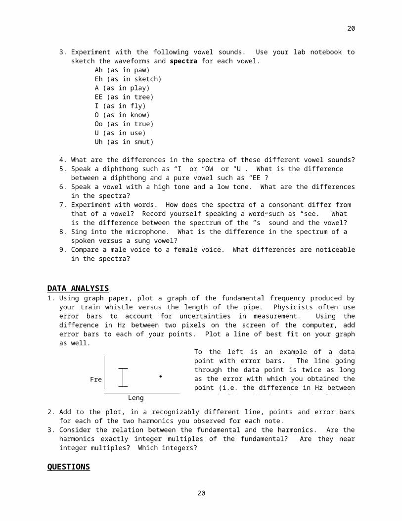
DATA ANALYSIS1. Using graph paper, plot a graph of the fundamental frequency produced by your train whistle versus the length

of the pipe. Physicists often use error bars to account for uncertainties in measurement. Using the difference in Hz between two pixels on the screen of the computer, add error bars to each of your points. Plot a line of best fit on your graph as well.

2. Add to the plot, in a recognizably different line, points and error bars for each of the two harmonics you observed for each note.

3. Consider the relation between the fundamental and the harmonics. Are the harmonics exactly integer multiples of the fundamental? Are they near integer multiples? Which integers?

QUESTIONS1. What kind of relationship did you find between frequency and length of the pipe? How might this

discovery relate to the equation at the beginning of the lab? Justify any observed deviations from the given equation.

2. For the whistle, what relationship could you determine existed between each fundamental and its two harmonics? Was there a ratio between each tone and its first and second visible harmonics?

3. When you spoke vowels at the same apparent pitch did the fundamental frequency shift at all? What does this tell you about the subjectivity of your sense of pitch?

4. Discuss the following: What is the difference in the spectrum of a spoken versus a sung vowel? Male vs Female voice? Consonant vs vowel? One vowel vs another?

5. What is the definition of a “diphthong”? What did you notice when trying to draw the waveforms of “diphthongs” like “I” and “U”?

6. Use what you learned about the train whistle to explore possible explanations for how the mouth changes to resonate at higher and lower pitches during speech.

15

15

To the left is an example of a data point with error bars. The line going through the data point is twice as long as the error with which you obtained the point (i.e. the difference in Hz between two pixels). Notice that the line is centered on the data point and the ends of the line are marked on both the top and bottom, so the error bars look like a capital “I.”Length

Freq.

Physics of MusicLab 3

Construction of a Flute(Last revised: Summer 2006 by Alice Quillen )

EQUIPMENT PVC pipe (last year we used ½ inch inside diameter (ID) pipe. The instructions require ¾ “ ID. I have now

found corks that fit this ID pipe. This end correction explains why the flutes from the ½” ID pipe are one semitone sharp.

Corks or dowels that fits into the end of the PVC pipe Rulers Tools: power hand-drills, drill bits, hacksaws, clamps, files, hammers, center punches, drill stops Mini vices Protective eyewear Tuners for measuring frequency Plumber’s goop for sealing the ends. Sandpaper Autobody filler and various goop for fixing mistakes. Mirror On wish list to buy: dremmel tool that works, awls, band-saw.Note: figures in this are from Hopkin’s book “Musical Instrument design.”

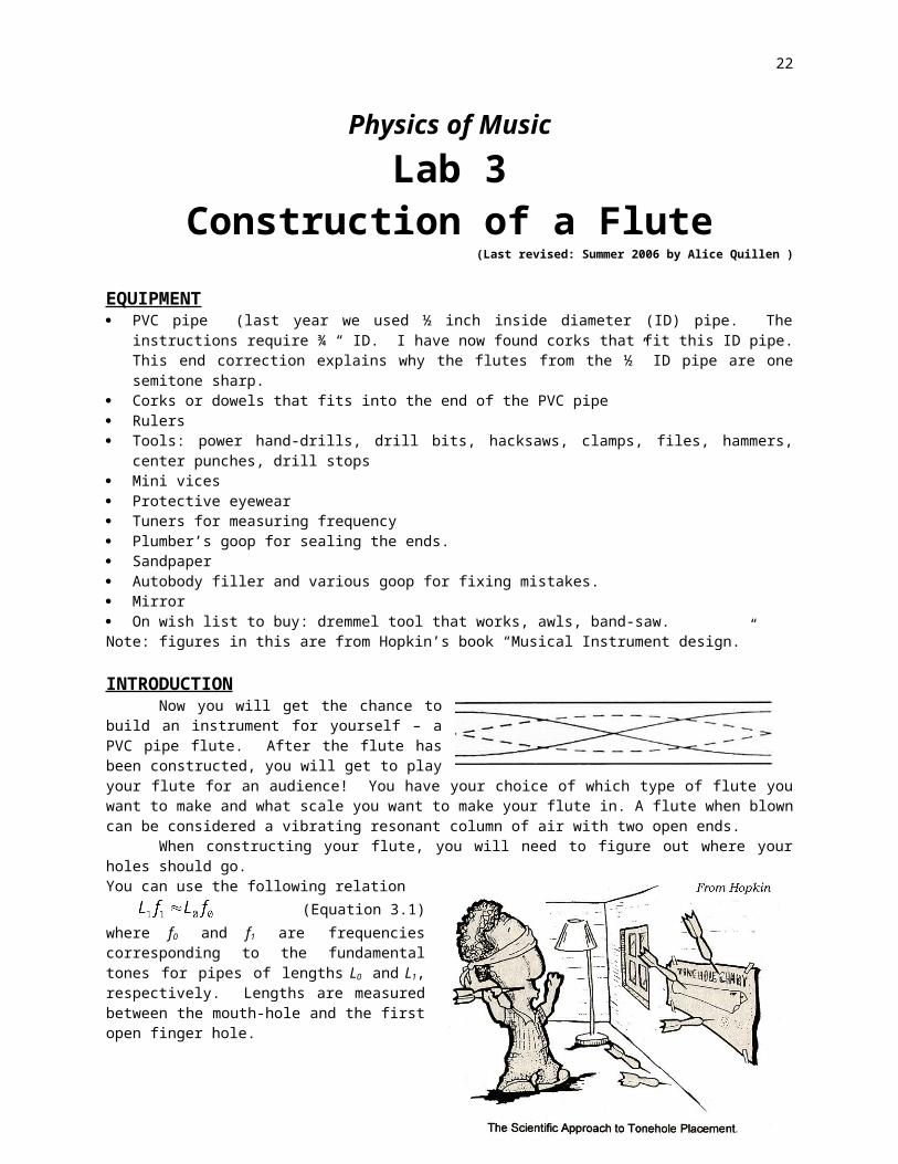
INTRODUCTIONNow you will get the chance to build an

instrument for yourself – a PVC pipe flute. After the flute has been constructed, you will get to play your flute for an audience! You have your choice of which type of flute you want to make and what scale you want to make your flute in. A flute when blown can be considered a vibrating resonant column of air with two open ends.

When constructing your flute, you will need to figure out where your holes should go.You can use the following relation

(Equation 3.1)where f0 and f1 are frequencies corresponding to the fundamental tones for pipes of lengths L0 and L1, respectively. Lengths are measured between the mouth-hole and the first open finger hole.

If you wish to make a flute in G, the hole placements are estimated below for you. They should approximately be consistent with the above equations. In your report you could compare the frequencies predicted from the above two equations and those you actually measure. Unfortunately the above two equations do not exactly predict the actual notes played by a flute. The diameter of the tube increases the effective length of the resonating tube (this is known as the end correction). A larger diameter hole decreases the effective length of the resonating tube so you can raise the pitch of a tone by enlarging a hole. Large tone-holes produce a larger volume of sound. Larger holes should also contribute to better tone quality by providing a tone richer in overtones or partials. Pitch measurement: Pitches are commonly measured with respect to the frequencies of the tempered scale with a concert A of 440Hz. These frequencies are listed in the table below and in Appendix C. Tuners usually give the

16

16

nearest note on the tempered scale and the difference between this not and the one you played. This difference is given in cents. Cents are defined in the following way: There are 100 cents in each half tone, and twelve half tones in an octave. So there are 1200 cents in an octave. An octave corresponds to frequency change of a factor of two. In other words a second note that is an octave above a first note has twice the frequency of the first. Consequently 1

cent corresponds to a factor of . If you are sharp by +21 cents you multiply the frequency of the nearest

tempered scale note by to calculate the actual frequency of your note. If you are flat by +18 cents you would

multiple by a factor of .

PURPOSEThe purpose of this lab is to learn how to use your knowledge of physics and music to construct an actual

musical instrument. It is quite difficult to make a flute that is easy to play and that can play notes that are in tune. In this lab you will discover the limitations of the simple numerical estimates for pitch (that given by the above equations). By creating this instrument we can perhaps gain respect and admiration for the design and redesign effort that went into some common musical instruments.

PROCEDURE

Sideblown Flute(There is a helpful insert on page 19)

1. Cut your PVC tubing to 16 and 7/16 inches. 2. Mold 1” of cork or dowel so it fits tightly in the end of the tube. This can be done by using a knife or by

using a sharp pipe of the same diameter as your tube to shape your cork. You may need to cut the cork so that it only sticks in ½” (according to the instructions).

3. Tap the cork or dowel into one end, to a depth of ½ an inch.

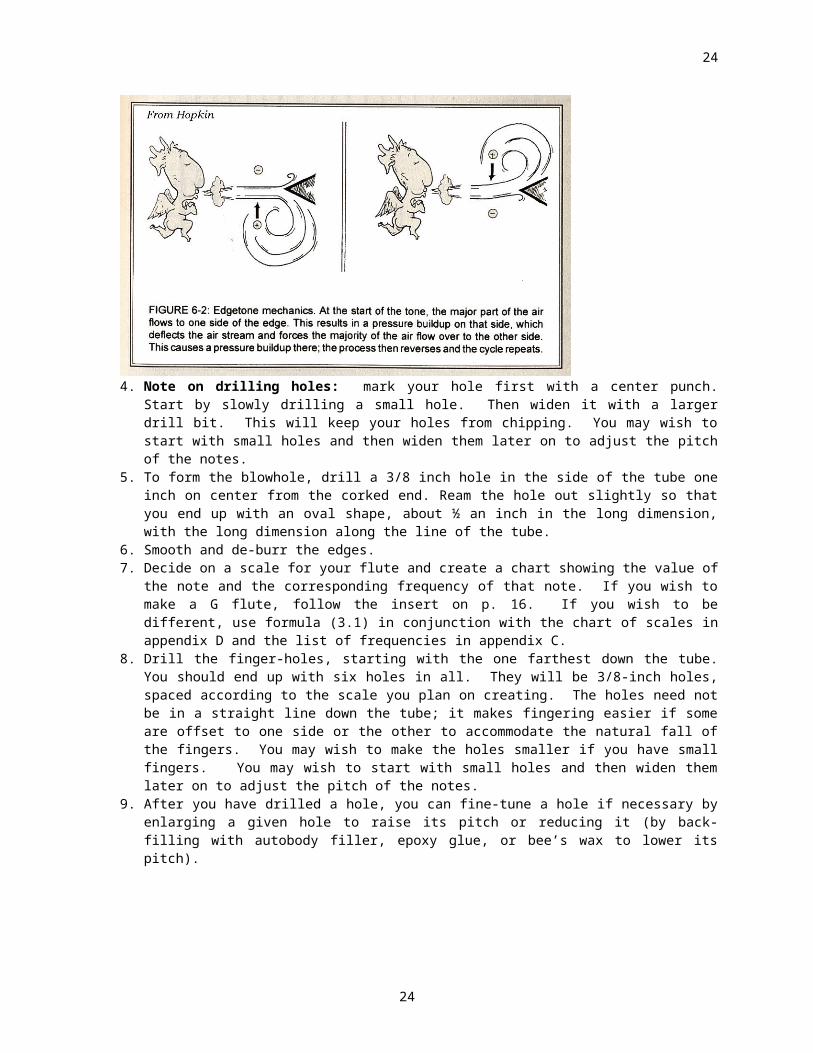
4. Note on drilling holes: mark your hole first with a center punch. Start by slowly drilling a small hole. Then widen it with a larger drill bit. This will keep your holes from chipping. You may wish to start with small holes and then widen them later on to adjust the pitch of the notes.

5. To form the blowhole, drill a 3/8 inch hole in the side of the tube one inch on center from the corked end. Ream the hole out slightly so that you end up with an oval shape, about ½ an inch in the long dimension, with the long dimension along the line of the tube.

6. Smooth and de-burr the edges.7. Decide on a scale for your flute and create a chart showing the value of the note and the corresponding

frequency of that note. If you wish to make a G flute, follow the insert on p. 16. If you wish to be

17

17

different, use formula (3.1) in conjunction with the chart of scales in appendix D and the list of frequencies in appendix C.

8. Drill the finger-holes, starting with the one farthest down the tube. You should end up with six holes in all. They will be 3/8-inch holes, spaced according to the scale you plan on creating. The holes need not be in a straight line down the tube; it makes fingering easier if some are offset to one side or the other to accommodate the natural fall of the fingers. You may wish to make the holes smaller if you have small fingers. You may wish to start with small holes and then widen them later on to adjust the pitch of the notes.

9. After you have drilled a hole, you can fine-tune a hole if necessary by enlarging a given hole to raise its pitch or reducing it (by back-filling with autobody filler, epoxy glue, or bee’s wax to lower its pitch).

10. Tape can be used to block extra holes. Note: PVC is cheap and plentiful. You can scrap your flute and try again if you screw up.

11. After you have drilled all the holes, practice playing your flute. You need to blow so that your air-stream hits the opposite edge of the mouth-hole. Place the flute against your lips and turn the flute back and forth while blowing until you can hear a breathy note. Adjust the angle of the flute and the way you blow until the note becomes stronger and purer. First play the highest note (no fingers down). Then slowly block each hole till you reach the lowest note. If one hole is leaking even a little bit you will not be able to play the lowest notes.

12. The stopper position of the cork or dowel can also be used to fine-tune. This adjustment should primarily affect the pitches of the higher notes.

13. After you have drilled all holes and learned to play the flute, measure the pitches of each note you can play. The uncovered holes do affect the pitches of notes blown. To measure the pitches of the notes, play your flute while looking at a tuner. Or you can play your flute while recording and then use the frequency analysis tool in Adobe/Audition as a tuner. You may need to adjust the length of the FFT for a pitch to be estimated. The pitch should appear on the top of the frequency analysis window. Here is an example of the format used by tuners: C4-10. The first letter is the nearest note on the tempered scale. The second note is the octave (4 is that begun by middle C on the piano). The last note is the number of cents the note is above or below the pitch of the note. In this example the note is -10 cents below C4. Write down in your notebook your pitch measurements.

14. Convert your note measurements to frequencies. Note: if you use Adobe/Audition you can directly measure the frequencies by clicking on the fundamental peak in the frequency analysis plot.

15. Write in your notebook the number of cents that each note is off. Then use the list of frequencies (given here and in Appendix C) to determine the actual frequencies of the notes. For example if you recorded C4+15, do the following:

You know by appendix C or the table given here that the C note is supposed to be 261.63 Hz.You know that you are off by +15 cents. By looking at the formula in “The 12 Tone Music Scale” table, you can calculate:15 cents = 1200 Log 2[f/261.63] where Log is base 2Or 15 cents = 3986 Log 10[f/261.63] where Log is base 10.

Frequencies of Notes in the Tempered Scale 4th octaveNote Frequency

(Hz)C4 261.63C# (D)4 277.18D4 293.66D# (E)4 311.13E4 329.63F4 349.23F#(G)4 369.99G4 392.00G#(A)4 415.30A4 440.00A#(B)4 466.16B4 493.88To predict the notes in the octave above this multiple the above frequencies by two. To predict the notes in the octave below this, divide the above frequencies by two.

18

18

So, the actual frequency of the note is 263.9Hz.

16. Practice playing your flute and see if you can get a clear tone at each note. To play more expressively try blowing a vibrato.

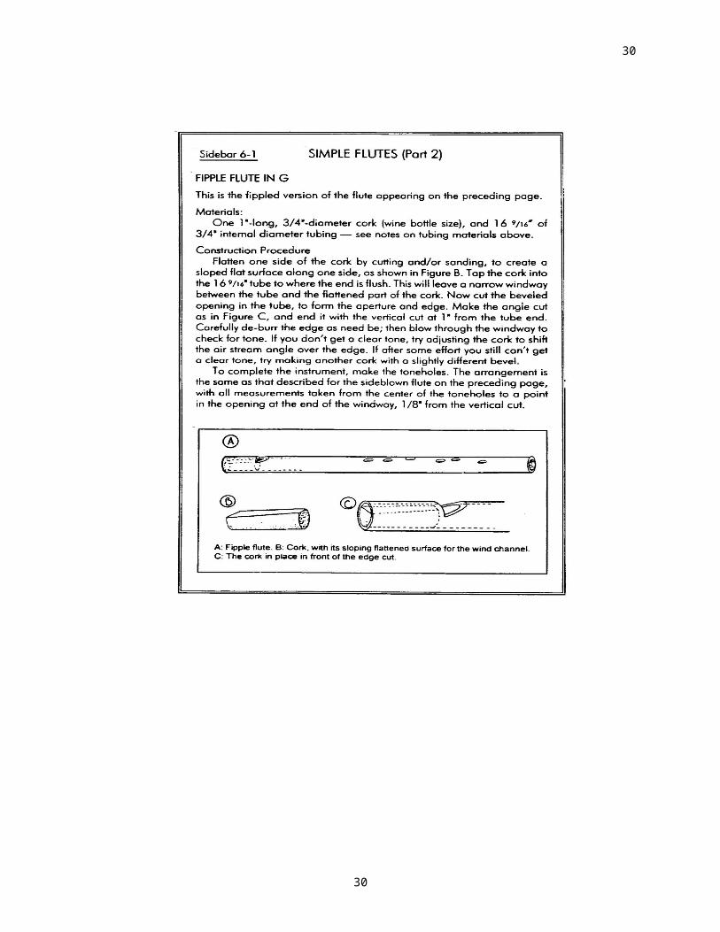
Fipple Flute (optional or instead of side-blown flute)(There is a helpful insert on page 20)

1. Flatten one side of your cork by cutting and/or sanding, to create a sloped flat surface along one side.2. Cut your PVC tubing to 16 and 9/16 inches.3. Tap the cork into one end of your tube so that the end is flush. This will leave a narrow windway between

the tube and the flattened part of the cork.4. Cut the beveled opening in the tube, to form the aperture and edge. Make the angle cut as shown in the

figure and end it with the vertical cut at one inch from the tube end.5. Carefully de-burr the edge as need be.6. Blow through the windway to check for tone. If you don’t get a clear tone, try adjusting the cork to shift

the air stream angle over the edge. If after some effort you still can’t get a clear tone, try making another cork with a slightly different bevel.

7. Decide on a scale for your flute and create a chart showing the value of the note and the corresponding frequency of that note.

8. Drill the fingerholes, starting with the one farthest down the tube. You should end up with six holes in all. They will be 3/8-inch holes, spaced according to the scale you plan on creating. Use formula (3.1) to determine the placement of your holes. The holes need not be in a straight line down the tube; it makes fingering easier if some are offset to one side or the other to accommodate the natural fall of the fingers.

9. After you have drilled a hole, you can fine-tune a hole if necessary by enlarging a given hole to raise its pitch or reducing it (by back-filling with autobody filler, epoxy glue, or bee’s wax) to lower its pitch.

10. The stopper position of the cork can also be used to fine-tune if you still need to do so after you have drilled all of your holes.

11. Write down (in your data notebook) the actual frequencies of the notes in your flute’s scale.12. Practice playing your flute and be sure that you can get a clear tone from each one of your holes.

DATA ANALYSIS1. If you made a G flute: Use equation (3.1) to determine the theoretical hole placement for your flute.

Make a table with the theoretical hole placement (found with the equation) in one column and the actual

19

19

hole placement (where the holes actually are on your flute) in another column. Be sure to demonstrate how to use equation (3.1) by showing your work for at least one calculation. If you made a flute with a different scale: demonstrate how you decided where you drilled your holes by applying formula (3.1) or (3.2). Make a table of these values. Be sure to show your work for at least one calculation.

2. Make a table listing the theoretical frequencies of the scale of your flute, the actual frequencies you obtained for the notes in your scale, and the number of cents you were off for each note. Consider making a plot or graph that shows these measurements.

QUESTIONS1. Is your flute accurate? What would you have done differently to increase the accuracy if you were to make

another flute?2. Are their trends in the differences between predicted and actual frequencies? Do your measured

frequencies tend to be higher or lower than the predicted values. Are the high notes further off than the low notes?

3. What was the most difficult part of constructing the flute? Can you think of ways that this part could have been done easier?

4. Have you found playing your flute to be difficult? What techniques have you used to generate a tone from your flute?

20

20

21

21

22

22

Physics of MusicLab 4 (Sonometer Lab)

Variations on Standing Waves(Last revised: Summer 2006 by Alice)

EQUIPMENT Pasco sonometers (pick up 5 from Thang) BK Precision function generators (pick up 5) Pasco counter/timers Tenma oscilloscopes Tuners Chladni plates, sine wave generators, mechanical drivers Scale

INTRODUCTIONMany musical instruments, such as guitars, pianos, and violins, operate by creating standing waves in

strings. This process has much in common with the creation of standing waves in tubes, as you will examine in the next lab. The formula for the frequency is given by the following formula:

(Equation 4.1)

This formula explains the relationship between the length L of the string and the frequencies fn at which the string will resonate. Here n is an integer. The lowest mode would have n=1. Two features of the equation should be noted. First, the string is fixed at both ends, which is mathematically equivalent to a tube that is open or closed at both ends. Second, the velocity of the sound wave is determined by qualities of the string. The velocity of sound is given by the following equation:

(Equation 4.2)

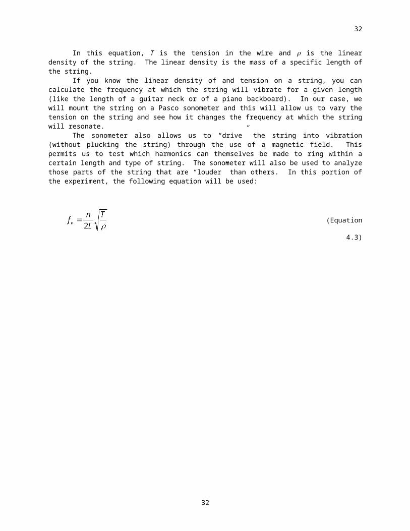
In this equation, T is the tension in the wire and is the linear density of the string. The linear density is the mass of a specific length of the string.

If you know the linear density of and tension on a string, you can calculate the frequency at which the string will vibrate for a given length (like the length of a guitar neck or of a piano backboard). In our case, we will mount the string on a Pasco sonometer and this will allow us to vary the tension on the string and see how it changes the frequency at which the string will resonate.

The sonometer also allows us to “drive” the string into vibration (without plucking the string) through the use of a magnetic field. This permits us to test which harmonics can themselves be made to ring within a certain length and type of string. The sonometer will also be used to analyze those parts of the string that are “louder” than others. In this portion of the experiment, the following equation will be used:

(Equation 4.3)

23

23

The formula for the tension applied to the string is:

(Equation 4.4)

where m is the mass on the end of the string and g is the gravitational constant. Notch number one is the notch closest to the sonometer string, while notch five is that farthest from the sonometer string.

In the second part of the experiment, the Chladni plates will demonstrate wave patterns on a stretched membrane. The plates represent percussion instruments such as the drum.

PURPOSEThe purpose of this lab is to analyze the relationship between mass and frequency in a vibrating string and

to look at the vibrations of different Chladni plates. PROCEDUREPart I – Sonometer

1. Use the scale provided to determine the mass of the string and a yardstick to measure its length from bridge to bridge (in meters). The linear mass density is the mass divided by the length of the string. If the linear mass density of the string is already known, then the TA will provide this information and you may skip this step.

2. The sonometer will be set up for you by your TA. Make sure the oscilloscope is on dual mode. The trigger should be for CH 2, DC. If you are not getting a signal, check the DC offset on the function generator. Make sure the driver is plugged into the GND and OUT on the function generator. You will hang your three different trial masses from the end of the sonometer’s tension rod. In the fifth notch, the tension applied to the string will be given by formula (4.4). Position the driver 5 cm from the bridge and the detector near the center. Attach 1 kg of mass to the end of the sonometer and record this value on your data sheet. In addition, record the length of the portion of the string that is resonating on your data sheet.

3. Use the instrument tuner to estimate the starting frequency of resonance (The frequency of resonance occurs when the string is plucked.) Set your function generator approximately 50 Hz below the frequency of resonance. The function generator will attempt to magnetically “drive” the string at the rate you have set. Slowly increase frequency until you find the first point at which the string resonates. You will know that the string is resonating because you will hear the string vibrating and you will observe a change in the waveform displayed by the pickup on your oscilloscope. Remember, the pickup and “driver” both create magnetic fields, so if you see a perfect sine wave coming from the pickup, you know that you are seeing traces of the driving signal. The real resonance will be a more complex waveform. Read this frequency from the counter/timer and record it on your data sheet.

4. Continue to increase the frequency until you find several more resonating frequencies and record these on your data sheet. Do not go past 1000 Hz. These resonating points will correspond to the string vibrating with two, three, and four nodes respectively. Move slowly here and try not to miss a resonant frequency between two others. It is easy to skip over a crucial point!

5. Repeat the above procedure using the third and first notch.

Part II – Chladni Plates1. You will be observing both the round and square chladni plates.2. Using the setup provided, sprinkle some sand on top of one of the plates. Make sure the plate is level.3. Increase the frequency slowly starting at around 10 Hz. When you find a pattern start to form with the sand

on the plate, note the frequency and draw the pattern on your data sheet.4. Continue until you have found several patterns. 5. Repeat process for the second plate.

DATA ANALYSIS1. Make two plots. First, plot the tension of the mass attached to the end of the string against the frequencies

at which the string vibrated. Make three unconnected points – one for the fundamental, and one for each

24

24

15

3sonometer

harmonic.) With three trials, you should be able to see a non-linear relationship between the tension and the frequencies of vibration. Next, plot the square root of the tension against the frequencies at which this tension allowed the string to resonate. In this plot, estimate a line of best fit.

2. Using the length of the string, the string tension, and the linear mass density, calculate the fundamental (n = 1) frequency of vibration for each of the three trials. How does this theoretical model compare to the resonant frequencies observed? Show your work.

3. From your experiments with the Chladni plates, make a chart showing the pattern observed and the frequencies at which you observed these patterns.

QUESTIONS1. Does your second plot confirm that the frequency is linearly proportional to the square root of tension and

thus the square root of mass?2. When you varied your pickup location, did you see any difference in output amplitude? Explain.3. Knowing what factors go into changing the resonant frequencies of a string, how can you make that low

string on your booty-shaking bass go even lower? Give at least three examples.4. When you were using the Chladni plates, were some patterns harder to create than others? What is the

difference between patterns on the circular plate and those on the square plate?

25

25

Physics of MusicLab 5

Resonant Tones in a Column of Air(Last revised: August 2005 by Alice Quillen)

EQUIPMENT Kundt’s tube apparatus (pick up 5 from Thang) PC and software 1 pair Headphones Tuning forks PASCO Sine wave generators and open speakers Meter stick Thermometer Masking tape

INTRODUCTIONAll wind instruments operate on the same basic principle. They all have a method of creating vibrations.

For example, a French horn player buzzes her lips and a clarinetist makes a wooden reed vibrate. All wind instruments have a characteristic length that determines what notes or vibrations can be produced by the instrument. Finally, they all have some type of device to project the sound that they produce. It is the second item in this list that we are concerned with here – the characteristic length. Only certain resonant frequencies can be produced in a tube of a particular length. Understanding the boundary conditions of a column of air will determine these frequencies.

Above are shown the fundamental modes of a column of air with two open ends (left) and one open, open closed end (right). We can calculate the allowable frequencies of a column of air by using the formulas:

(open-open) or (closed-open) (Equations 6.1)

In the above formulas, f is the frequency, v is the speed of sound in air, and L is the tube length. The allowed frequencies are known as harmonics of the tube. The velocity depends on the temperature in the room, as you have already demonstrated in your homework. Be sure to use the correct form of the equation for the boundary conditions you are considering!

In the first part of the lab, we will use a tuning fork to create longitudinal vibrations that are transmitted through the air into a plastic tube with an adjustable piston at one end. By subtly adjusting the length of the air column via moving the piston, standing waves are produced in the tube. The lengths of the air columns that produce resonance determine the location of the nodes of the standing waves. Knowing the distance between the nodes, the frequency can be calculated using equations (5.1).

In the second part of the lab, we will use a setup similar to that of part one. Instead of a tuning fork, we will use a pair of headphones driven by the frequency generator built into your Pasco box. We will detect resonance

26

26

in two ways: with our ears and with the oscilloscope. Instead of adjusting the length of the tube with the piston, we will vary the driving frequency of the speaker and use a tube that is open at both ends.

PURPOSEThe purpose of this lab is to examine the resonant frequencies of a closed and open tube.

PROCEDUREPart I – The Open/Closed Tube

1. Set up the apparatus as demonstrated by your TA.2. The TA will divide up the tuning forks among the groups. After you have finished using your tuning forks,

you will switch with another group so that you will eventually use all of the tuning forks. Record the frequencies of the tuning forks you are given on your data sheet.

3. Firmly strike the tuning fork with a rubber mallet or the bottom of your sneaker (should you be wearing one) and hold it about a centimeter away from the open end of the tube. Do not strike the tuning forks on the table! Be sure not to let it touch the tube.

4. Vary the effective length of the tube by moving the piston through its complete range and determine the positions of the nodes by listening for resonance points. In general, the larger the tuning fork you are working with, the harder it will be to locate the resonance points. Listen closely!

5. Record the distance of each node from the open end of the tube. 6. Note the temperature in the lab.7. Repeat the above procedure until you have worked with every tuning fork.

Part II – The Open/Open Tube1. Prop your sound sensor next to the end of your tube and hold your headphones next to the support at the

other end of your tube. Be careful not to “close off” either end of your tube (or else you may alter your data).

2. Connect your sound sensor to channel C and your headphones to channel A.3. Start your Pasco software and open the signal generator by clicking on the sample button. Drag an analog

plug to channel C and select the “sound sensor” icon.4. Drag a “scope” to channel C.5. Set the signal generator to create a frequency lower than 150 Hz. Click the ON button and then click the

MON button to begin viewing the sound at the end of your tube on the cope.6. Increase the frequency slowly until you find resonance. You will both hear the intensity of the sound

increase and see the trace on the scope increase in amplitude. You may need to adjust the vertical sweep of the scope as the sound coming from the headphones is not that loud. This isn’t all that easy, so be patient. Once you find resonance, record the frequency from the counter/timer.

7. Continue increasing the frequency to find 4 or 5 more resonance points.8. Measure the length of the tube and record it on your data sheet.

DATA ANALYSIS1. For part one, calculate the frequency of each tuning fork using equations (5.1). Do this for each set of data

you took. For example, first calculate the frequency using the first resonance point and then using the second, and so on making sure to make the appropriate adjustments to the formula. Be sure to use the correct form of the equation! One is for an open tube, and the other is for a closed tube!

2. Calculate the theoretical harmonic spectrum of the open tube.3. For part one, make a table with one column the calculated spectrum and another column the measured

spectrum.4. For part two, make a table with the calculated spectrum in one column and the measured spectrum in the

other column.

QUESTIONS1. When you calculated the frequency of each tuning fork in part one, did each set of data for one tuning fork

give the same frequency? Why or why not? How do these calculated frequencies compare to the actual (labeled) frequencies of the tuning forks?

27

27

2. When you constructed the two tables above, did you find any discrepancies between the calculated spectrum and the measured spectrum? How do you account for this?

3. A stopped organ pipe has a stopper in the top of it, forcing a node to be there. Why do think organ makers’ use stopped pipes when they are building organs, especially for smaller buildings?

4. In this lab, we studied the resonant properties of a cylindrical tube. What do you think would change if we had a conical “tube”?

5. What effect would an increase in air temperature have on your results in this experiment? Explain.6. The tunnel below the Eastman Quad at the UR is approximately 50 meters long. What frequencies would

resonate in this tube? Are there any frequencies that would resonate in the tunnel below your range of hearing?

Notes: The speakers sometimes produce frequencies an octave above that at which driven.

28

28

Physics of Music

Lab 6 Room Acoustics

(Last revised: Oct 2005 by Alice Quillen)

EQUIPMENT

Meter stick and Tape measure Noise level meter (dB meter) Noise making devices (pieces of wood for clappers, optional balloons and thumbtacks). Continuous single frequency noise makers (signal generator attached to speaker or computer with a synthesized

sine wave). Use the sine generator +speaker for the padded closet. Use the amplifier and signal generator for the hall. Use one of the computers to generate the sounds for the lab. Someday we will get more equipment and this will be easier.

Microphones, stands, preamps connected to computers running Adobe Audition. Extra microphone cables so the microphones can reach the padded closet and hallway.

INTRODUCTIONOne important application of the study of sound is in the area of acoustics. The complete acoustical

analysis of a room is both difficult and time-consuming. The benefits of such an analysis, however, are tremendous for lecture halls, auditoriums, and libraries where the sound level is an important feature of the room. What we plan to do in this lab is give you an introduction to room acoustics by listening and recording the way sound travels in rooms. There are three rooms we can easily study near the lab: the lab itself, the “anechoic” chamber (i.e. padded closet across the hall, B+L417C, that isn’t actually very anechoic) and the hallway (which really carries echoes). Anechoic means no echoes. An anechoic chamber is a room built specifically for the purpose of absorbing sound. Such a room should be considerably quieter than a normal room. Step into the padded closet and snap your fingers and speak a few words. The sound should be muffled. For those of us living in Rochester this will not be a new sensation as freshly fallen snow absorbs sound very well. If you close your eyes you could almost imagine that you are outside in the snow (except for the warmth, and bizarre smell in there).

The reverberant sound in an auditorium dies away with time as the sound energy is absorbed by multiple interactions with the surfaces of the room. In a more reflective room, it will take longer for the sound to die away and the room is said to be 'live'. In a very absorbent room, the sound will die away quickly and the room will be described as acoustically 'dead'. But the time for reverberation to completely die away will depend upon how loud the sound was to begin with, and will also depend upon the acuity of the hearing of the observer. In order to provide a reproducible parameter, a standard reverberation time has been defined as the time for the sound to die away to a level 60 decibels below its original level. The reverberation time, RT60, is the time to drop 60 dB below the original level of the sound. The reverberation time can be measured using a sharp loud impulsive sound such as a gunshot, balloon popping or a clap.

Why use 60dB to measure the reverberation time? The reverberation time is perceived as the time for the sound to die away after the sound source ceases, but that of course depends upon the intensity of the sound. To have a reproducible parameter to characterize an auditorium which is independent of the intensity of the test sound, it is necessary to define a standard reverberation time in terms of the drop in intensity from the original level, i.e., to define it in terms of relative intensity. The choice of the relative intensity to use is of course arbitrary, but there is a good rationale for using 60 dB since the loudest crescendo for most orchestral music is about 100 dB and a typical room background level for a good music-making area is about 40 dB. Thus the standard reverberation time is seen to be about the time for the loudest crescendo of the orchestra to die away to the level of the room background. The 60 dB range is about the range of dynamic levels for orchestral music.

What is a good reverberation time for a room? If you are using the room for lectures (speech) then a long reverberation time makes it difficult for the audience to understand words. However long reverberation times are

29

29

desirable for example in churches for organ music. Reflective surfaces lengthen the reverberation time whereas absorption surfaces shorten it. A larger room usually has a longer reverberation time. Rooms that are good for both speech and music typically have reverberation times between 1.5 and 2 seconds. The reverberation time is strongly influenced by the absorption coefficients of the surfaces in a room, but it also depends upon the volume of the room. You won't get a long reverberation time with a small room.

Predicting the reverberation time and Sabine’s formula.Sabine is credited with modeling the reverberation time with the simple relationship which is called the

Sabine formula:

(Equation 7.1)

You use the 0.16 sec/m if you are working in meters. You use the 0.049 sec/foot if you are working in ft. Here V is the volume of the room and Se is an effective area. The effective area is calculated as follows

Here each area Si has an absorption coefficient ai. The effective area is a sum of areas, Si , each with its own absorption coefficient ai. These areas are the surfaces in the room (ceiling, walls, floor, people, etc…). Another way to write the effective area is with a sum

Note you must put the areas (Si ) in the same units as the volume V (meter2 for area and meter3 for volume or ft2 for area and ft3 for volume). When a sound wave in a room strikes a surface, a certain fraction of it is absorbed, and a certain amount is transmitted into the surface. Both of these amounts are lost from the room, and the fractional loss is characterized by an absorption coefficient, a, which can take values between 0 and 1, 1 being a perfect absorber and 0 being a perfect reflector. Absorption coefficients are unitless. The absorption coefficient is the fraction of the power absorbed in one reflection. Absorption coefficients for some common materials are given below. The absorption coefficient of a surface can depend on the frequency of sound used to measure it. For example, carpet is quit absorptive at high frequencies but not at low frequencies. A perfectly absorptive room would have an effective area that is equal to the total surface area of its walls, ceiling and floor. A highly reflective room would have an effective area that is smaller than its total surface area.

The Sabine formula works reasonably well for medium sized auditoriums but is not to be taken as an exact relationship. The Sabine formula neglects air absorption, which can be significant for large auditoriums. It also tends to overestimate the reverberation times for enclosures of high absorption coefficient. A better approximation for such enclosures utilizes an overall average absorption coefficient:

(equation 7.2)

where S is the total surface area of the room. Note that this reduces the calculated reverberation time.

Some important acoustical characteristics to consider are:

Liveness – This just refers to the length of the reverberation time. The longer the reverberation time, the more “live” the room is.

Intimacy – This refers to how close the performing group sounds to the listener. Fullness – This refers to the amount of reflected sound intensity relative to the intensity of the

direct sound. The more reflected sound, the more fullness the room will have. Clarity – This is the opposite of fullness. In general, greater clarity implies a shorter

reverberation time. Warmth – This is obtained when the reverberation time for low-frequency sounds is somewhat

greater than the reverberation time for high frequencies. Brilliance – This is the opposite of warmth. Texture – This refers to the time structure of the pattern in which the reflections reach the

listener. The first reflection should quickly follow the direct sound.

30

30

Blend – This refers to how well the mixing of sound occurs between all of the instruments playing.

Ensemble – This refers to the ability of the members of the performing group to hear each other during the performance.

Some problems in acoustical design are: Focusing of sound – This refers to the undesirable effect that occurs when sound is much louder

at one point in the room than surrounding points in the room. Echoes – To obtain good texture, it is desirable to avoid any particularly large single echoes. Shadows – These are quiet areas that can be produced when there are large overhanging

balconies or other structure jutting into the room. Resonances – It is necessary to separate the resonances of a speaker and the box enclosure of a

tuned-port system to provide the best sound. External noise – This refers to noise coming from outside of the room. Double-valued reverberation time – If a recording of a musical event is played back in a room

that it was not originally recorded in, this phenomenon can result.

Absorption coefficients for common surfaces:

Effective areas for people and seats in auditoriums in sabins120Hz 250Hz 500Hz 1000Hz 2000Hz 5000Hz

Audience per person in sabins 0.35 0.43 0.47 0.50 0.55 0.60

Auditorium seat, solid un-upholstered

0.02 0.03 0.03 0.03 0.04 0.04

Auditorium seat, upholstered 0.3 0.3 0.3 0.3 0.35 0.35

A sabin is a unit of acoustic absorption equivalent to the absorption by a square foot of a surface that absorbs all incident sound.

31

31

PURPOSEThe purpose of this lab is to explore the acoustics of three different rooms. We will compare the

characteristics of three rooms: the hallway, the lab (B+L403), and the padded closet (B+L417C) (aka “anechoic chamber”). Your lab session should divide into three groups. Each lab group will study a separate room. Afterwards the different lab groups can combine their measurements to compare the characteristics of each room. In this lab you will listen to sounds in each room. You will measure the loudness at different locations in the room using a dB meter. You will measure the loudness at different locations with a continuous single frequency noise being played in the room to see if there are any acoustic shadows in the room. You will measure the reverberation time of the room and compare your measured value to that estimated using Sabine’s formula.

PROCEDUREA. Listening

1. By listening compare the characteristics of the three rooms: the hallway, the lab (B+L403), and the padded closet (B+L417C). Snap your fingers, carry out a conversation, sing, clap some boards together. Describe the characteristics of these room in terms of the above vocabulary (brilliance, liveness, clarity, warmth, etc..).

B. Measuring the Reverberation Time1. Go to the room that your lab group has chosen to study.2. To record a quickly decaying sound you need to adjust the recording level so that the sound is not heavily

saturated or clipped. Bring up Adobe Audition on your computer and make sure that the preamp is plugged in. You can look as the sound level by right clicking on the level meter (bottom of screen) and choosing “Monitor Record Level.” Make a loud clap with two pieces of wood. Check that the sound is not saturated. Adjust the preamp to a good level. Record a few claps. Check that the sound is not heavily clipped. Play back your sound to hear what it sounds like. You want to hear the room not the clapper so make the claps distant from the microphone (on the other side of the room).

To show the sound level before recording select Monitor Record Level. To get this box right click on the sound level bar at the bottom of the screen. Adjust the preamp knobs so that a clap is well measured (not too faint) but is also not heavily clipped (or in the red zone).

3. Look at the waveform of your recorded claps. Expand the horizontal or time axis using the zoom button at the bottom of the screen (this looks like a little plus sign inside a circle). Take a look at the decay of the sound that you recorded.

32

32

An example of a clap. Each spike is an echo from a different surface in the room. Large flat surfaces produce large strong echoes.

4. Are there any particularly strong echoes in your room? Can you see them in the waveform of your recorded claps?

5. Make sure the time format is set so that you can record the time with precision (to a precession of msecs). Click on “View” at the top of the program, select “Display Time Format” and choose “Decimal”.

6. Measuring the loudness at a particular time. With a left click and drag, select a region of your waveform. Write down the start time of your selected region.

A selected region of the waveform.

7. On the top of the screen there are a bunch of options. Choose “Analyze”. Choose “Statistics”. Adjust the “Window width” to something small such as 1ms. Press the button that says “Recalculate RMS.” The window width is the time over which each power measurement is made. You should make the window width small enough that your selected region contains many windows. The Average or RMS power is the average of all the powers measured in each window. RMS stands for root mean square. Remember the power depends on the square of the signal. The RMS power is given in dBFS which is dB below full scale. This arbitrarily sets 0dB to be the largest number that you can measure. The beginning of the clap should be near 0dB (nearly clipped). As the sound decays you should measure lower values of the RMS power (that means negative values of dB).

The Waveform Statistics box. Using this box you can measure the loudness in dB at a particular time.

33

33

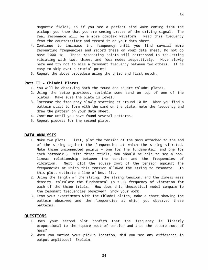
8. Record the power levels at different times after the onset of the clap. Use the RMS power as a measure of the power. Remember dB is decibel or 10 log10 (Power).9. Plot dB level vs time. You should see points that lie along a line. The power is decaying exponentially in time. However dB is the logarithm of the power so we expect a line on a plot of dB vs time. 10. It is impractical to directly measure RT60 or how long it takes to drop 60 dB below the loudest level. This would correspond to a drop of a factor of a million in the power of the noise. What prevents us from measuring the sound level over such a large range? We can’t measure noise fainter than the ambient background noise (you will measure this in part D below). Also the analog to digital converter on the sound card in the computer doesn’t have enough bits to cover this large a dynamic range. How are we going to calculate RT60 if we can’t measure the sound when it is 60 dB fainter? We can assume that the decay of the sound follows a line when plotted as dB vs time. You can describe this kind of decay as an exponential decay. Using your plot of dB vs time, extend your line and estimate how long it would take for your sound to decay to 60dB below that of the loudest part. This time is then an estimate for the reverberation time or RT60. This technique is called extrapolation.

C. Predicting the reverberation time using Sabine’s formula.1. Using the various measuring devices, measure the volume of the room. If your room is not rectangular, be

sure to make enough measurements so that you are able to calculate the volume. Note:floor tiles in the US tend to be 1ft square.

2. Measure the surface area of all the different absorbing materials in the room. Remember to include yourself if you happen to be in the room! If you have a large number of similar objects, it suffices to measure the surface area of one of them and multiply. For example, if you are measuring the surface area of seats in an auditorium, measure one seat and multiply that value by the number of seats in the auditorium. There is no need to measure the surface area of everything in the room, but all of the larger objects should be measured. Don’t forget to measure doorways, windows, and yourselves.

1. Calculate the affective area of your room, Ae, using absorption coefficients listed above or from the appendix of your lab manual. If a material in you room is not found on the chart, make a guess at what the absorption coefficient is based on what material it is most like on the list. For people use the table above that gives affective areas per person in sabins (units ft squared).

3. Predict the reverberation time using Sabine’s formula. Predict the reverberation time for two different frequencies.

4. Does your predicted RT60 agree with the one you measured? A clap has a fairly flat spectrum (both high frequency and low frequency components). This makes it hard to do this comparison exactly. What other effects might account for any difference between your predicted and measured value for the reverberation time?

D. Searching for dead-spots and measuring loudness as a function of frequency Is this lab too long? Then maybe qualitatively do this part (do it for fun and don’t bother taking measurements).

1. Make a map of your room. Make your map as specific as possible by indicating what objects are in the room and where they are found.

2. Determine the ambient noise level at different locations in the room using the sound level meter. Ambient noise is the noise that a room naturally has in it due to such things as air conditioners, lights, and sound

34

34

from nearby rooms and hallways. Record the dB values, where you measured them and which way you pointed the dB meter when you took the measurements.

3. Play a single pitch continuous sound at a low frequency (few hundred Hz). Record the loudness (dB level) at different locations in the room. Make a note of where you produce the sound and where you record the loudness level.

4. Play a single pitch continuous sound at a high frequency (few thousand Hz). Record the loudness (dB level) at different locations in the room.

5. Are there any differences between loudness levels measured at different frequencies? Remember that a difference in dB corresponds to a multiplicative factor in power. You may have a louder sound at one frequency than another. However the change in dB level from one location to another tells you about a change in power. You can compare the change in dB level measured at two locations using one frequency sound to the change in dB level measured at two locations using a different frequency sound.

6. Were you able to find any “dead spots” in your room? These are places where the sound level meter recorded significantly lower values than at surrounding points when a sound was played from a fixed point in the room. If you did find any, can you see any reason why they are there? Indicate them on your map of your room.

Additional QuestionsCompare your results with the other groups in your lab session. Listen to their recorded claps. Did you each predict the same reverberation time? How are the three rooms different? What are the differences in the predicted reverberation times from the three rooms? What are the differences in the measured reverberation times from the three rooms?

Notes:To remove DC offset that might have been introduced in recording: Select the entire waveform. Choose “Effects”. Choose “Filters”. Choose “Scientific Filters”. Do a High Pass filter with a cutoff of 10Hz. This should remove a DC offset. You can now set the vertical scale to dB and have a sensible zero level.

Note the appendix gives absorption effective areas for people and auditorium seats. These are given in sabins. A sabin is a unit of acoustic absorption equivalent to the absorption by a square foot of a surface that absorbs all incident sound.

35

35

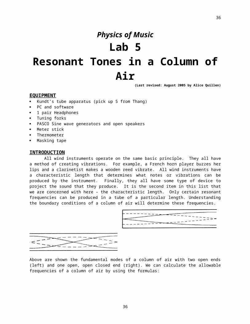
Physics of MusicLab 7

Copper Pipe Xylophone(Last revised: Summer 06 by Alice Quillen)

EQUIPMENT

Copper pipes in a scale at ½” diameter Different diameter pipes with same lengths Mallets Stands for the copper pipes Tuners Microphones, stands, preamps connected to computers running Adobe Audition.

INTRODUCTION

For a guitar string or a column of air, the pitch of the fundamental tone sounded is proportional to the length of the string or length of the column of air. However for other systems the pitch of the fundamental tone may depend on the length in a more complicated manner. For example the pitch of the fundament may depend on the square of the length or the square root of the length. In this lab we will experimentally measure the way that the fundamental tone of copper pipe depends on its length. We can write

Equation 5.1where f is the frequency of the fundamental tone, L is the length of the pipe and is a power that will be measured in this lab. The symbol means “is proportional to”. For guitar strings and flutes, and the pitch of the fundamental tone is proportional to the length of the string or column of air.

For a guitar string or a column of air, the overtones are integer multiples of the fundamental tone. However there are vibrating systems where the overtones are not integer multiples. This contributes to their timbre. Bells, drums and copper pipes are examples of instruments that have a complex spectrum of overtones. In this lab you will measure the frequencies of these overtones, fn and their ratios to that of the fundamental or fn/f1. x

The modes excited when a copper pipe depend on the speed of sound in the pipe and the stiffness of the pipe. A different diameter pipe should have a different stiffness (harder to bend) and so should have different frequencies of vibration.

PROCEDUREA. Pitch as a function of length.

1. Using the ½” pipes at different lengths. Hit the pipes and measure their fundamental pitches.

2. Compute the frequencies of these tones.3. Measure the lengths of the pipes.

36

36

4. What is the relation between pipe length and pitch? Does the frequency depend linearly on the length of the pipe? What is your best estimate for in equation 5.1?

B. Pitch as a function of pipe diameter and material1. Measure the fundamental frequencies for two pipes of the same material (copper) but

different diameters.2. Suggest a relationship between pipe diameter and fundamental frequency?3. Measure the fundamental frequency for two pipes of the same length and approximately

same diameter but different material (steel and copper).

C. Structure of Overtones for one pipe 1. Record the sounds from the pipes. Measure the frequencies of the overtones. Are they

integer multiples of the fundamental?2. The sound of the pipe may depend upon where you hold the pipe or where you hit it.

Record while you hit the pipe in different locations or hold the pipe at different locations. Does the frequency spectrum change?

3. Where is the optimum location to hold the pipe so that the fundamental rings the longest?4. Measure the overtones for the two pipes of different diameters but the same length.

Compute the ratios of the overtones divided by the fundamental. Are these ratios the same for the two different diameter pipes?

5. Repeat for the steal pipe.6. Measure the overtones for the largest and smallest length ½” pipes. Compute the ratios

of the overtones divided by the fundamental. Are these ratios the same for the two different diameter pipes?

7.

D. Discussion1. Discuss the relation between the fundamental pitch and pipe length, the fundamental

pitch and pipe diameter and the fundamental pitch and pipe material. We might expect stiffer pipes to have higher frequency fundamentals.

2. Discuss the differences you see in the harmonics for the different pipes.

37

37

Appendix A. Acoustics Insert with Helpful Information:

A sabin is a unit of acoustic absorption equivalent to the absorption by a square foot of a surface that absorbs all incident sound.

38

38

Appendix B: Scientific Notation and its PrefixesSI PREFIXES

Factor Prefix Symbol1024 yotta Y

1021 zetta Z

1018 exa E

1015 peta P

1012 tera T

109 giga G

106 mega M

103 kilo k

102 hecto h

101 deka da

10-1 deci d

10-2 centi c

10-3 milli m

10-6 micro

10-9 nano n

10-12 pico p

10-15 femto f

10-18 atto a

10-21 zepto z

10-24 yocto y

Examples of use:89 ns = 89 10-9 s = 8.9 10-8 s230 km = 230 103 m = 2.3 105 m

39

39

Appendix C: Notes on the Piano

40

40

C0 16.352 C3 130.81 C6

41

41

C0#/D0 17.342 138.59D0 18.354D0#/E0E0F0F0#/G0G0G0#/A0A0A0#/B0B0

42

42

Appendix D: Equal Tempered Music Scale

43

43

Appendix E: The 12 Pitch Classes

\

44

44

Appendix F: The speed of sound in air

V = 331.4 + 0.6 Tc where V is the speed of sound in m/s and Tc is the air temperature in Celcius.This is a good approximation at sea level.

45

45