PHYSICS OF MANTLE CONVECTION

Yanick RicardLaboratoire de Science de la Terre

Universite de Lyon; Universite de Lyon 1; CNRS; Ecole Normale Superieure de Lyon,2 rue Raphael Dubois, 69622, Villeurbanne Cedex, France.

abstract This chapter presents the fundamental equations necessaryto under-stand the physics of fluids and some applications to mantle convection. The firstsection derives the equations of conservation for mass, momentum and energy,and the boundary and interface conditions for the various variables. The thermo-dynamic and rheological properties of solids are discussedin the second section.The mechanism of thermal convection and the classical Boussinesq and anelas-tic approximations are presented in the third section. As the subject is not oftenincluded in geophysical text books, an introduction to the physics of multicom-ponent and multiphase flows is given in a fourth section. At last the specifics ofmantle convection are reviewed in the fifth section.

Contents

1 Introduction 4

2 Conservation equations 52.1 General expression of conservation equations . . . . . . . .. . . 52.2 Mass conservation . . . . . . . . . . . . . . . . . . . . . . . . . . 72.3 Momentum conservation . . . . . . . . . . . . . . . . . . . . . . 8

2.3.1 General momentum conservation . . . . . . . . . . . . . 82.3.2 Inertia and non-Galilean forces . . . . . . . . . . . . . . . 92.3.3 Angular momentum conservation . . . . . . . . . . . . . 11

2.4 Energy conservation . . . . . . . . . . . . . . . . . . . . . . . . 122.4.1 First law and internal energy . . . . . . . . . . . . . . . . 122.4.2 State variables . . . . . . . . . . . . . . . . . . . . . . . 132.4.3 Temperature . . . . . . . . . . . . . . . . . . . . . . . . 142.4.4 Second law and entropy . . . . . . . . . . . . . . . . . . 15

1

2.5 Gravitational forces . . . . . . . . . . . . . . . . . . . . . . . . . 172.5.1 Poisson equation . . . . . . . . . . . . . . . . . . . . . . 172.5.2 Self-gravitation . . . . . . . . . . . . . . . . . . . . . . . 172.5.3 Conservative forms of momentum and energy equations .18

2.6 Boundary and interface conditions . . . . . . . . . . . . . . . . . 202.6.1 General method . . . . . . . . . . . . . . . . . . . . . . . 202.6.2 Interface conditions in the 1D case and for bounded vari-

ables . . . . . . . . . . . . . . . . . . . . . . . . . . . . 222.6.3 Phase change interfaces . . . . . . . . . . . . . . . . . . 222.6.4 Weakly deformable surface of a convective cell . . . . . .24

3 Thermodynamic and rheological properties 253.1 Equation of State and solid properties . . . . . . . . . . . . . . .253.2 Rheology . . . . . . . . . . . . . . . . . . . . . . . . . . . . . . 28

3.2.1 Elasticity . . . . . . . . . . . . . . . . . . . . . . . . . . 283.2.2 Viscous Newtonian rheology . . . . . . . . . . . . . . . . 293.2.3 Maxwellian Visco-elasticity . . . . . . . . . . . . . . . . 303.2.4 Non-linear rheologies . . . . . . . . . . . . . . . . . . . . 32

4 Physics of convection 344.1 Convection experiments . . . . . . . . . . . . . . . . . . . . . . . 344.2 Basic balance . . . . . . . . . . . . . . . . . . . . . . . . . . . . 354.3 Two simple solutions . . . . . . . . . . . . . . . . . . . . . . . . 36

4.3.1 The diffusive solution . . . . . . . . . . . . . . . . . . . 364.3.2 The adiabatic solution . . . . . . . . . . . . . . . . . . . 374.3.3 Stability of the adiabatic gradient . . . . . . . . . . . . . 38

4.4 Approximate equations . . . . . . . . . . . . . . . . . . . . . . . 394.4.1 Depth dependent reference profiles . . . . . . . . . . . . 394.4.2 Nondimensionalization . . . . . . . . . . . . . . . . . . . 404.4.3 Anelastic approximation . . . . . . . . . . . . . . . . . . 424.4.4 Dimensionless numbers . . . . . . . . . . . . . . . . . . 434.4.5 Boussinesq approximation . . . . . . . . . . . . . . . . . 444.4.6 Internal heating . . . . . . . . . . . . . . . . . . . . . . . 454.4.7 Alternative forms . . . . . . . . . . . . . . . . . . . . . . 454.4.8 Change of nondimensionalization . . . . . . . . . . . . . 47

4.5 Linear stability analysis for basally heated convection . . . . . . . 474.6 Road to chaos . . . . . . . . . . . . . . . . . . . . . . . . . . . . 49

5 Introduction to physics of multicomponent and multiphaseflows 515.1 Fluid dynamics of multicomponent flows in solution . . . . .. . 53

5.1.1 Mass conservation in a multicomponent solution . . . . .53

2

5.1.2 Momentum and energy in a multicomponent solution . . . 545.1.3 Entropy conservation in a multicomponent solution . .. . 565.1.4 Advection-diffusion equation and reaction rates . . .. . . 575.1.5 Conservation properties of the advection-diffusionequation 605.1.6 Laminar and turbulent stirring . . . . . . . . . . . . . . . 625.1.7 Diffusion in Lagrangian coordinates . . . . . . . . . . . . 63

5.2 Fluid dynamics of two phase flows . . . . . . . . . . . . . . . . . 655.2.1 Mass conservation for matrix and fluid . . . . . . . . . . 665.2.2 Momentum conservation of matrix and fluid . . . . . . . . 675.2.3 Energy conservation for two-phase flows . . . . . . . . . 695.2.4 Phenomenological laws . . . . . . . . . . . . . . . . . . 705.2.5 Summary equations . . . . . . . . . . . . . . . . . . . . . 73

6 Specifics of Earth’s mantle convection 756.1 A mantle without inertia . . . . . . . . . . . . . . . . . . . . . . 75

6.1.1 Dynamic models . . . . . . . . . . . . . . . . . . . . . . 756.1.2 Mantle flow and post-glacial models . . . . . . . . . . . . 766.1.3 Time dependent models . . . . . . . . . . . . . . . . . . 77

6.2 A mantle with internal heating . . . . . . . . . . . . . . . . . . . 796.3 A complex rheology . . . . . . . . . . . . . . . . . . . . . . . . 80

6.3.1 Temperature dependence of viscosity . . . . . . . . . . . 826.3.2 Depth-dependence of viscosity . . . . . . . . . . . . . . . 836.3.3 Stress-dependence of viscosity . . . . . . . . . . . . . . . 846.3.4 Grain size dependence of viscosity . . . . . . . . . . . . . 84

6.4 Importance of sphericity . . . . . . . . . . . . . . . . . . . . . . 856.5 Other depth-dependent parameters . . . . . . . . . . . . . . . . . 85

6.5.1 Thermal expansivity variations . . . . . . . . . . . . . . . 856.5.2 Increase in average density with depth . . . . . . . . . . . 876.5.3 Thermal conductivity variations . . . . . . . . . . . . . . 88

6.6 Thermo-chemical convection . . . . . . . . . . . . . . . . . . . . 886.7 A complex lithosphere: plates and continents . . . . . . . . .. . 90

3

1 Introduction

In many text books of fluid dynamics, and for most students, the word “fluid”refers to one of the states of matter, either liquid or gaseous, in contrast to thesolid state. This definition is much too restrictive. In fact, the definition of afluid rests in its ability to deform. Basically any material that appears as non-deformable in most common life experiments, with a crystalline structure (i.e.,belonging to the solid state) or with a disordered structure(e.g., a glass, that froma thermodynamic point of view belongs to the liquid state) can be deformed whensubjected to stresses for a long enough time.

The characteristic time constant of the geological processes related to mantleconvection, typically 10 Myrs (3×1014 s), is so long that the mantle, althoughstronger than steel and able to transmit seismic shear waves, can be treated asa fluid. Similarly, ice, which is the solid form of water, is able to flow frommountain tops to valleys in the form of glaciers. A formalismthat was developedfor ordinary liquids or gases can therefore be used in order to study the insideof planets. It is not the equations themselves, but their parameters (viscosity,conductivity, spatial dimensions...) that characterize their applicability to mantledynamics.

Most materials can therefore behave like elastic solids on very short time con-stants and like liquids at long times. The characteristic time that controls theappropriate rheological behavior is the ratio between viscosity, µ, and elasticity(shear modulus),µr, called Maxwell timeτM (Maxwell, 1831-1879),

τM =µ

µr

. (1)

The rheological transition in some materials like silicon occurs in only a few min-utes; a silicon ball can bounce on the floor, but it turns into apuddle when left ona table for tens of minutes. The transition time is of the order of a few hundredyears for the mantle (see 3.2). Phenomena of a shorter duration than this timewill experience the mantle as an elastic solid while most tectonic processes willexperience the mantle as irreversibly deformable. Surfaceloading of the Earthby glaciation and deglaciation involves times of a few thousands years for whichelastic aspects cannot be totally neglected with respect toviscous aspects.

Although the word “convection” is often reserved for flows driven by internalbuoyancy anomalies of thermal origin, in this chapter, we will more generally use“convection” for any motion of a fluid. Convection can be kinematically forcedby boundary conditions or induced by density variations. The density variationscan be of compositional or thermal origin. We will however, mostly focus on theaspects of thermal convection (or Rayleigh-Benard convection, (Rayleigh, 1842-1919; Benard, 1874-1939)) when the fluid motion is driven bythermal anomalies

4

and discuss several common approximations that are made in this case. We knowhowever that many aspects of mantle convection can be more complex and involvecompositional and petrological density anomalies or multi-phase physics. We willreview some of these complexities.

The physics of fluid behavior, like the physics of elasticityis based on the gen-eral continuum hypothesis. This hypothesis requires that parameters like density,temperature, or momentum are defined everywhere, continuously. This hypoth-esis seems natural for ordinary fluids at the laboratory scale. We will adopt thesame hypothesis for the mantle although we know that it is heterogeneous at var-ious scales and made of compositionally distinct grains.

2 Conservation equations

The basic equations of this section can be found in more detail in many classicaltext books (Batchelor, 1967;Landau and Lifchitz, 1980). We will only emphasizethe aspects that are pertinent for the Earth.

2.1 General expression of conservation equations

Let us consider a fluid transported by the velocity fieldv, a function of positionX and timet. There are two classical approaches to describe the physicsin thisdeformable medium. Any variableA in a flow, can be considered as a simplefunction of position and time,A(X, t), in a way very similar to the specificationof the electromagnetic field. This is the Eulerian point of view (Euler, 1707-1783).The second point of view is traditionally attributed to Lagrange (Lagrange, 1736-1813). It considers the trajectory that a material element of the flow initially atX0 would followX(X0, t). An observer following this trajectory would naturallychoose the variableA(X(X0, t), t). The same variableA seen by an Eulerianor a Lagrangian observer would have very different time-derivatives. For Eulerthe time derivative would simply be the rate of change seen byan observer at afixed position, i.e., the partial derivative∂/∂t. For Lagrange, the time derivativenoted withD would be the rate of change seen by an observer riding on a materialparticle

DA

Dt=dA(X(X0, t), t)

dt=∑

i=1,3

∂A

∂Xi

∂Xi

∂t+∂A

∂t, (2)

where theXi are the coordinates ofX. SinceX is the position of a material ele-ment of the flow, its partial time derivative is simply the flowvelocityv. The La-grangian derivative is also sometimes material called the derivative, total deriva-tive, or substantial derivative.

5

The previous relation was written for a scalar fieldA but it could easily beapplied to a vector fieldA. The Eulerian and Lagrangian time derivatives are thusrelated by the symbolic relation

D

Dt=

∂

∂t+ (v · ∇) (3)

The operator(v · ∇) is the symbolic vector(v1∂/∂x1, v2∂/∂x2, v3∂/∂x3) and aconvenient mnemonic is to interpret it as the scalar productof the velocity field bythe gradient operator(∂/∂x1, ∂/∂x2, ∂/∂x3). The operator(v ·∇) can be appliedto a scalar or a vector. Notice that(v · ∇)A is a vector that is neither parallel toA nor tov.

In a purely homogeneous fluid, the flow lines are not visible. In this case thepoint of view of Euler seems natural. On the other hand, a physicist describingelastic media can easily draw marks on the surface of deformable objects and flowlines become perceptible for him. He thus favors the Lagrangian point of view.We will mostly adopt the Eulerian perspective for the description of the mantle..However when we discuss deformation of heterogeneities embedded in and stirredby the convective mantle the Lagrangian point of view will bemore meaningful(see section 5.1.7).

A starting point for describing the physics of a continuum are the conservationequations. Consider a scalar or a vector extensive variableA (i.e., mass, momen-tum, energy, entropy, number of moles...) per unit volume and a virtual but fixedvolumeΩ enclosed in its boundaryΣ. This virtual volume is freely crossed by theflow. The temporal change ofA enclosed inΩ is

d

dt

∫

ΩA dV =

∫

Ω

∂A

∂tdV . (4)

SinceΩ is fixed, the derivative of the integral is indeed the integral of the partialtime derivative.

The total quantity of the extensive variableA in a volumeΩ can be related toa local production,HA (with units ofA per unit volume and unit time), and to thetransport (influx or outflux) ofA across the interface. This transport can eitherbe a macroscopic advective transport by the flow or a more indirect transport, forexample at a microscopic diffusive level. Let us callJA the total flux ofA per unitsurface area. The conservation ofA can be expressed in integral form as

∫

Ω

∂A

∂tdV = −

∫

ΣJA · dS +

∫

ΩHA dV , (5)

where the infinitesimal surface is oriented with the outwardunit normal. Equation(5) is the general form of any conservation equation. When the flux is regular

6

enough (when no surface of discontinuity crosses the volumeΩ), we can makeuse of the divergence theorem

∫

ΣJA · dS =

∫

Ω∇ · JA dV , (6)

to transform the surface integral into a volume integral. The divergence operatortransforms the vectorJ = (J1, J1, J2) into the scalar∇ · J =

∑

i=1,3 ∂Ji/∂xi,scalar product of the symbolic operator∇ by the real vectorJ (notice the differ-ence between the scalar∇ ·J and the operatorJ ·∇). Since the integral equation(5) has been written for any volumeΩ, we can deduce that the general differentialform of the conservation equation is,

∂A

∂t+ ∇ · JA = HA. (7)

A similar expression can be used for a vector quantityA with a tensor fluxJand a vector source termHA. In this case, the divergence operator converts thesecond-order tensor with componentsJij into a vector whose components are∑

j=1,3 ∂Jij/∂xj .We now apply this formalism to various physical quantities.Three quantities

are strictly conserved: the mass, the momentum and the energy. We must iden-tify the corresponding fluxes but no source terms should be present (in fact, inclassical mechanics the radioactivity appears as a source of energy). One veryimportant physical quantity is not conserved - the entropy -but the second law ofthermodynamics insures the positivity of the associated sources.

2.2 Mass conservation

The net rate at which mass is flowing is

Jρ = ρv. (8)

Using either the Eulerian or the Lagrangian time derivatives, the mass conserva-tion can be written

∂ρ

∂t+ ∇ · (ρv) = 0, (9)

orDρ

Dt+ ρ∇ · v = 0. (10)

In an incompressible fluid, the Lagrangian observer does notsee any density vari-ation andDρ/Dt = 0. In this case, mass conservation takes the simple form∇ · v = 0. This equation is commonly called the continuity equation althoughthis name is a little bit awkward.

7

Using mass conservation, a few identities can be derived that are very usefulfor transforming an equation of conservation for a quantityper unit mass to aquantity per unit volume. For example for any scalar fieldA,

∂(ρA)

∂t+ ∇ · (ρAv) =

D(ρA)

Dt+ ρA∇ · v = ρ

DA

Dt, (11)

and for any vector fieldA,

∂(ρA)

∂t+ ∇ · (ρA ⊗ v) =

D(ρA)

Dt+ ρA∇ · v = ρ

DA

Dt, (12)

whereA⊗ v is a tensor of componentsAivj . WhenA is a constant the equalities(11) corresponds to the two expressions of mass conservation (9) and (10).

2.3 Momentum conservation

2.3.1 General momentum conservation

The changes of momentum can be easily deduced by balancing the changes ofmomentum with the body forces acting in the volumeΩ and the surface forceacting on its surfaceΣ. The total momentum is

∫

Ωρv dV , (13)

and its variations are due to

• advective transport of momentum across the surfaceΣ,

• forces acting on this surface and, last,

• internal body forces.

The momentum conservation can therefore be expressed in integral form as∫

Ω

∂(ρv)

∂tdV = −

∫

Σρv(v · dS) +

∫

Σσ · dS +

∫

ΩF dV . (14)

By definition, the tensorσ corresponds to the total stresses applied on the surfaceΣ, (see Figure 1). The termF represents the sum of all body forces, and in partic-ular the gravitational forcesρg (we will not consider the electromagnetic forcesin this chapter).

Using the divergence theorem (for the first term of the right side, ρv(v · dS)can also be writtenρ(v ⊗ v) · dS) and the equality (12), the differential form ofmomentum conservation becomes

ρDv

Dt= ∇ · σ + F. (15)

8

−1 −0.5 0 0.5 1 1.5 2−1

−0.5

0

0.5

1

1.5

2

σyydxdz

σzydxdz

σxydxdz

x

y

z

o

Figure 1: The force per unit area applied on a surface directed by the normalvectorni is by definitionσ ·ni. The component of this force along the unit vectorej thereforeej · σ · ni.

It is usual to divide the total stress tensor into a thermodynamic pressure−P I

whereI is the identity stress tensor, and a velocity-dependent stressτ . The re-lationship between the tensorτ and the velocity field will be discussed later insection 3.2. Without motion, the total stress tensor is thusisotropic and equal tothe usual pressure. In all the geophysical literature, it has been assumed that thevelocity dependent tensor has no isotropic component, i.e., it is traceless tr(τ ) = 0or that tr(σ) = −3P (see section 3.2 for more details). The velocity-dependentstress tensorτ is thus also the deviatoric stress tensor.

As ∇ · (P I) = ∇P , momentum conservation (14), in terms of pressure anddeviatoric stresses is

ρDv

Dt= −∇P + ∇ · τ + F. (16)

This equation is called the Navier-Stokes equation (Navier, 1785-1836; Stokes,1819-1903) when the stress tensor is linearly related to thestrain rate tensor (see3.2).

2.3.2 Inertia and non-Galilean forces

In almost all studies of mantle dynamics the fact that the Earth is rotating is simplyneglected. It is however worth discussing this point. Let usdefine a reference

9

frame of vectorsei attached to the solid Earth. These vectors rotate with the Earthand with respect to a Galilean frame

dei

dt= ω × ei, (17)

whereω is the angular velocity of Earth’s rotation. A pointX =∑

iXiei of theEarth has therefore an accelerationγ in a Galilean frame (Galileo, 1564-1642)

γ =∂v

∂t+ 2ω × v + ω × (ω × X) +

dω

dt×X. (18)

In this well known expression, one recognizes on the right side, the accelerationin the non-Galilean Earth reference frame, the Coriolis, (Coriolis, 1792-1843),centrifugal and Poincare accelerations (Poincare, 1854-1912).

To quantify the importance of the three first acceleration terms (neglecting thePoincare term), let us consider a characteristic scale forlength (the Earth radiusa = 6371 km), and mantle velocity (U = 10 cm yr−1) and let us compare thevarious acceleration terms. One immediately gets

inertia

Coriolis=

U

2ωa=

1

2.9 × 1011, (19)

Coriolis

gravitational force=

2ωU

g=

1

2.1 × 1013, (20)

centrifugal

gravitational force=ω2a

g=

1

291. (21)

A first remark is that the inertial term is much smaller than the Coriolis term(this ratio is also known as the Rossby number, (Rossby, 1898-1957)). The Corio-lis term is itself perfectly negligible in front of the gravitational force. Even if weargue that a more meaningful comparison would be to compare the whole Coriolisforce2ρωU to the lateral variations of the gravitational forceδρg, (this ratio wouldbe the inverse of the Eckman number, (Eckman, 1874-1954)), inertia and Corio-lis accelerations play absolutely no role in mantle dynamics. Neglecting inertiameans neglecting the changes in kinetic energy as inertia isthe time-derivative ofthe kinetic energy. We can perform a simple numerical estimate to realize howridiculously small the mantle kinetic energy is. The kinetic energy of a litho-spheric plate (a square of size 2000 km, thickness 100 km, velocity 5 cm yr−1 anddensity 3000 kg m−3) is 1.5 kJ, comparable to that of a middle size car (2000 kg)driven at only 8 km h−1!

The centrifugal term is also quite small but not so small (1/291 of gravitationalforce). It controls two effects. The first is the Earth’s flattening with an equatorial

10

bulge of 21 km (1/300 of Earth’s radius). This is a static phenomenon that hasno interactions with convection dynamics. The second is thepossibility that thewhole planet rotates along an equatorial axis in order to keep its main inertial axiscoincident with its rotational axis (Spada et al., 1992;Ricard et al., 1993b). Thisrotational equilibrium of the Earth will not be discussed here (e.g., seeMunk andMacDonald(1960) for the dynamics of a deformable rotating body).

We neglect all the acceleration terms in the following but weshould rememberthat in addition to the convective motion of a non-rotating planet, a global rotationof the planet with respect to its rotation axis, is possible.This motion documentedby paleomagnetism, is called True Polar Wander (Besse and Courtillot, 1991).

2.3.3 Angular momentum conservation

The angular momentum per unit massJ = r × v is also a conserved quantity. Itsconservation law can be obtained by two different ways. First, as we did for massand momentum conservation, we can express the balance of angular momentum inintegral form. In the absence of intrinsic angular momentumsources, its variationsare due to

• advective transport of angular momentum across the surfaceΣ,

• torque of forces acting on this surface and, last,

• torque of internal body forces.

The resulting balance is therefore,∫

Ω

∂(ρJ)

∂tdV = −

∫

ΣρJ(v · dS) +

∫

Σr × (σ · dS) +

∫

Ωr × F dV . (22)

The only difficulty to transform this integral form into a local equation is with theintegral involving the stress tensor. After some algebra, the equation (22) becomes

ρDJ

Dt= r × ∇ · σ + r × F + T , (23)

where the torqueT is the vector(τzy −τyz , τxz −τzx, τyx −τxy). A second expres-sion can be obtained by the vectorial multiplication of the momentum equation(15) byr×. This expression,

ρDJ

Dt= r × ∇ · σ + r × F, (24)

differs from (23) by the absence of the torqueT . This proves that in the absenceof sources of angular momentum, the stress (eitherσ or τ ) must be representedby a symmetrical tensor,

σ = σt, τ = τ

t. (25)

where[ ]t denotes tensor transposition.

11

2.4 Energy conservation

2.4.1 First law and internal energy

The total energy per unit mass of a fluid is the sum of its internal energy,U , andits kinetic energy (this approach implies that the work of the various forces isseparately taken into account; another approach that we usein 2.5.3, adds to thetotal energy the various possible potential energies and ignores forces). In thefixed volumeΩ, the total energy is thus

∫

Ωρ(U +

v2

2) dV . (26)

A change of this energy content can be caused by

• advection of energy across the boundaryΣ by the macroscopic flow,

• transfer of energy through the same surface, but at a microscopic level

• work of body forces,

• work of surface forces, and, last

• radioactive heat production

Using the divergence theorem, the balance of energy can therefore be written

∂

∂t

(

ρ(U +v2

2)

)

= −∇ ·(

ρ(u+v2

2)v + q + Pv − τ · v

)

+F ·v+ρH, (27)

whereq is the diffusive flux,H the rate of energy production per unit mass andwhere the stresses are divided into thermodynamic pressureand velocity depen-dent stresses.

This expression can can be developed and simplified by using the equality (11)and the equations of mass and momentum conservation, (9) and(16) to reach theform

ρDUDt

= −∇ · q − P∇ · v + τ : ∇v + ρH. (28)

The viscous dissipation termτ : ∇v is the contraction of the two tensorsτ and∇v. Its expression is

∑

ij τij∂vi/∂xj (be careful with the difference between thescalar∇ · v and the tensor∇v of components∂vi/∂xj).

12

2.4.2 State variables

The internal energy can be expressed in terms of the more usual thermodynamicstate variables, namely, temperature, pressure and volume. We use volume tofollow the classical thermodynamics presentation, but since we apply thermody-namics per unit mass, the volumeV is in fact the volume per unit mass or1/ρ.We use the first Law that states that during an infinitesimal process the variation ofinternal energy is the sum of the heatδQ and workδW exchanged. Although irre-versible processes occur in the fluid, we assume that we can adopt the hypothesisof local thermodynamic equilibrium.

The exchanges of heat and work are not exact differentials: the entire preciseprocess has to be known to compute these exchanges, not only the initial and finalstages. Using eitherT − V or T − P variables, we can write

δQ = CV dT + ldV = CPdT + hdP, (29)

whereCP anCV are the heat capacities at constant pressure and volume andhand l are two other calorimetric coefficients necessary to account for the heatexchanges at constant temperature. In the formalism of the physics of fluids theexchange of work is only due to the work of pressure forces

δW = −PdV. (30)

This implies that only the pressure term corresponds to an energy capable to bestored and returned without loss when the volume change is reversed. On the con-trary the stresses related to the velocity will ultimately appear in the dissipative,irrecoverable term of viscous dissipation. This point willbe further commentedin the section 3.2 about rheology.

Thermodynamics states that the total variations of energy,dU = δQ + δW ,enthalpy,dH = dU+d(PV ) or entropy,dS = δQ/T , are exact differentials. Thismeans that the difference in energy (enthalpy, entropy) between an initial and afinal state only depends of the initial and final states themselves, not the inter-mediate stages. This implies mathematically that their second partial derivativeswith respect to any pair of variables are independent of the order of differentiation.Using these rules a large number of equalities can be derivedamong the thermo-dynamic coefficients and their derivatives. These are called the Maxwell relationsand are discussed in most thermodynamics textbooks (e.g.,Poirier, 1991, ). Wecan in particular derive the values ofl andh,

l = αTKT , and h = −αTρ. (31)

13

In these expressions forl andh, we introduced the thermal expansivityα and theisothermal incompressibilityKT ,

α =1

V

(

∂V

∂T

)

P

= −1

ρ

(

∂ρ

∂T

)

P

,

KT = − V

(

∂P

∂V

)

T

= ρ

(

∂P

∂ρ

)

T

.

(32)

The thermodynamic laws and differentials apply to a closed deformable vol-umeΩ(t). This corresponds to the perspective of Lagrange. We can thereforeinterpret the differential symbols ”d” of the thermodynamic definitions (29) of(30) as Lagrangian derivatives ”D”.

To summarize, when the expressions forl andh are taken into account, (31),and when the differential symbols are interpreted as Lagrangian derivatives, thefirst law,dU = δQ+ δW can be recast as

DUDt

= CVDT

Dt+ (αTKT − P )

∇ · vρ

, (33)

or asDUDt

= CPDT

Dt− αT

ρ

DP

Dt− P

∇ · vρ

. (34)

In these equations we also have replaced the volume variation using mass conser-vation (9)

DV

Dt=D(1/ρ)

Dt= − 1

ρ2

Dρ

Dt=

∇ · vρ

. (35)

2.4.3 Temperature

We can now identify these two thermodynamic equations (33) or (34), with ourconservation equation deduced from fluid mechanics, (28), to express the conser-vation of energy in terms of temperature variations

ρCPDT

Dt= − ∇ · q + αT

DP

Dt+ τ : ∇v + ρH,

ρCVDT

Dt= − ∇ · q − αTKT∇ · v + τ : ∇v + ρH.

(36)

In these two equivalent expressions, in addition to diffusion, three sources of tem-perature variations appear on the right side. The last termρH is the source of ra-dioactive heat production. This term is of prime importancefor the mantle, mostlyheated by the decay of radioactive elements like235U, 238U, 236Th and40K. All to-gether these nuclides generate about20 × 1012 W (McDonough and Sun, 1995).

14

Although this number may seem large, it is in fact very small.Since the Earth nowhas about6×109 inhabitants, the total natural radioactivity of the Earth is only∼3kW/person, not enough to run the appliances of a standard kitchen in a developedcountry. It is amazing that this ridiculously small energy drives the plates, raisesmountains and produces a magnetic field. In addition to the present-day radioac-tivity, extinct radioactivities, like that of36Al (with a half life of 0.73 Myr), haveplayed an important role in the initial stage of planet formation (Lee et al., 1976).

The viscous dissipation termτ : ∇v converts mechanical energy into a tem-perature increase. This term explains the classical Joule experiment (equivalencebetween work and heat, (Joule, 1818-1889)) in which the potential energy of aload (measured in joules), drives a propeller in a fluid, and dissipates the mechan-ical energy as thermal energy (measured in calories). The same dissipative termexplains why clay (e.g., silly putty) heats when kneaded in our hands.

The remaining source term, containing the thermodynamic coefficients (α orαKT in (36)), cancels when the fluid is incompressible (e.g., whenα = 0 or when∇ ·v = 0). This term is related to adiabatic compression and will be discussed insection 4.3.2.

2.4.4 Second law and entropy

We now apply the second law of thermodynamics and first express the entropyconservation law. Assuming local thermodynamic equilibrium, we havedU =TdS − PdV . Using the equation of conservation for the internal energyU , (28),and expressing the volume change in term of velocity divergence (35), we obtain

ρTDSDt

= −∇ · q + τ : ∇v + ρH. (37)

To identify the entropy sources, we can express this equation in the form of aconservation equation (see (7)),

∂(ρS)

∂t= −∇ ·

(

ρSv +q

T

)

− 1

T 2q · ∇T +

1

Tτ : ∇v +

1

TρH. (38)

The physical meaning of this equation is therefore that the change of entropy isrelated to a flux of advected and diffused entropy,ρsv andq/T , to radioactiveproduction and to two other production terms.

A brief introduction to the general principles of non-equilibrium thermody-namics will be given in 5.1.4. Here, we simply state that the second law requiresthat in all situations, the total entropy production is positive. When the entropyterms are of different tensor orders (tensors, vectors or scalars), the fact that theyare affected differently by a change of coordinates, implies for isotropic systemsthat the production terms of different tensor orders must separately be positive.

15

This is called the Curie principle (Curie, 1859-1906) (see e.g.,de Groot and Mazur(1984);Woods(1975)). It implies that

−q · ∇T ≥ 0, and τ : ∇v ≥ 0. (39)

The usual Fourier law (Fourier, 1768-1830) with a positive thermal conductivityk > 0,

q = −k∇T, (40)

satisfies the second law.When the conductivityk is uniform, the thermal diffusion term of the energy

equation−∇ ·q becomesk∇2T where∇2 = ∇ ·∇ is the scalar Laplacian oper-ator (Laplace, 1749-1827). Instead of a thermal conductivity, a thermal diffusivityκ can be introduced

κ =k

ρCP, (41)

(in principle isobaric and isochoric thermal diffusivities should be defined). Insituations with uniform conductivity, without motion and radioactivity sources,the energy equation (36) becomes the standard diffusion equation

∂T

∂t= κ∇2T. (42)

The relation between stress and velocity will be discussed in detail in section3.2. We will show that the relationship

τ = 2µ(

ǫ− 1

3∇ · v

)

(43)

is appropriate for the mantle, where the strain rate tensorǫ is defined by

ǫ =1

2

(

[∇v] + [∇v]t)

. (44)

Using this relation and assumingµ uniform, the divergence of the stress tensorthat appears in the momentum conservation equation has the simple form

∇ · τ = µ∇2v +

µ

3∇(∇ · v), (45)

where the vectorial Laplacien∇2 stands for∇(∇·) − ∇ × (∇×). This rela-tionship suggests a meaningful interpretation of the viscosity. The momentumequation (16), can be written

∂v

∂t=µ

ρ∇

2v + other terms.... (46)

16

forgetting the other terms, a comparison with the thermal diffusion equation (42)shows that the kinematic viscosityν, defined by

ν =µ

ρ, (47)

should rather be called the momentum diffusivity; it plays the same role withrespect to the velocity as thermal diffusivity does with respect to temperature.

2.5 Gravitational forces

2.5.1 Poisson equation

In this chapter, the only force is the gravitational body force. The gravity is thesum of this gravitational body force and the centrifugal force already discussed(see 2.3.2). The gravitational force per unit mass is the gradient of the gravitationalpotentialψ, a solution of Poisson’s equation (Poisson, 1781-1840)

g = −∇ψ, and ∇2ψ = 4πGρ, (48)

whereG is the gravitational constant (some textbooks define−ψ as the gravita-tional potential). In the force term that appears in the momentum equation (16),F = ρg, the gravitational force per unit mass should be in agreement with thedistribution of masses: the Earth should be self-gravitating.

2.5.2 Self-gravitation

When dealing with fluid dynamics at the laboratory scale, thegravitational forcecan be considered as constant. The gravitational force is related to the entiredistribution of mass in the Earth (in the Universe) and is practically independent ofthe local changes in density in the experimental room. Therefore, at the laboratoryscale, it is reasonable to forget Poisson’s equation and to assume thatg = g0, auniform and constant reference gravitational field.

Inside a planet, the density can be divided into an average depth-dependentdensity,ρ0(r), the source of the reference depth-dependent gravitational field,g0(r), and a density perturbationδρ, origin of a gravitational perturbationδg.The force term,F is thereforeρ0g0 + δρg0 + ρ0δg at first order. It is tempting toassume that each term in the previous expression is much larger than the next oneand hopefully that only the first two terms are of importance (neglecting the sec-ond term would suppress any feed back between density perturbations and flow).Practically, this would imply consideration of the total density anomalies but onlythe depth dependent gravitational field. Solving Poisson’sequation to computethe perturbed gravitational field would thus be avoided.

17

We can test the above idea and show that unfortunately the third term, namelythe force due to the perturbation of gravitation acting on the average density, maybe of the same order as the second one (Ricard et al., 1984;Richards and Hager,1984;Panasyuk et al., 1996). To perform this exercise we have to introduce thespherical harmonic functionsYlm(θ, φ). These functions of latitudeθ and longi-tudeφ oscillate on a sphere just like 2D sinusoidal functions on a plane. Eachharmonic function changes signl − m times from North to South pole, andmtimes over the same angle (180 degrees) around the equator. The degreel can thusbe interpreted as corresponding to a wavelength of order2πa/l. Spherical har-monics constitute a basis for functions defined on the sphereand are also eigen-functions of the angular part of Laplace’s equation which allows an easy solutionof Poisson’s equation.

Let us consider a density anomalyδρ = σδ(r − a)Ylm(θ, φ) at the surface ofa sphere of radiusa and uniform densityρ0 (δ(r − a) is the Dirac delta function(Dirac, 1902-1984),σ has unit of kg m−2). This mass distribution generates theradial gravitational perturbation field inside the planet

δg = 4πGσl

2l + 1

(

r

a

)l−1

Ylm(θ, φ), (49)

We can compare the termsρ0〈δg〉 and g0〈δρ〉, both averaged over the planetradius. For a uniform planet, the surface gravitational force per unit mass isg0 = 4/3πGρ0a. Since〈δρ〉 = σYlm(θ, φ), we get

ρ0〈δg〉g0〈δρ〉

=3

2l + 1. (50)

This estimate is certainly crude and a precise computation taking into account adistributed density distribution could be done. However this rule of thumb wouldremain valid. At low degree the effect of self-gravitationρ0δg is about 50% ofthe direct effectδρg0 and reaches 10% of it only nearl ∼ 15. Self-gravitationhas been taken into account in various models intended to explain the Earth’sgravity field from mantle density anomalies (see Chapter 7 and Chapter 8 of thisTreatise). Some spherical convection codes seem to neglectthis effect although itis important at the longest wavelengths.

2.5.3 Conservative forms of momentum and energy equations

In the general remarks on conservation laws in section 2.1, we wrote that con-served quantities like mass, momentum and energy can only betransported but donot have production terms (contrary to entropy). However, in the momentum con-servation (16) and in the energy conservation (27) two terms, ρg andρg ·v, appear

18

as sources (we also said that the radioactive termρH, appears because the classi-cal physics does not identify mass and energy. A negligible term−ρH/c2, wherec is the speed of light, should, moreover, be present in the mass conservation).

It is interesting to check that our equations can be recast into an exact conser-vative form. An advantage of writing equations in conservative form is that sucha form is appropriate to deal with global balance, interfaces and boundaries (seesection 2.6). We can obtain conservative equations by usingPoisson’s relationand performing some algebra

ρg = − 1

4πG∇ ·

(

g ⊗ g − 1

2g2I

)

(51)

ρg · v = −ρDψDt

− 1

4πG∇ ·

(

g∂ψ

∂t

)

− 1

8πG

∂g2

∂t(52)

If we substitute these two expressions in the momentum and the energy conserva-tion equations, (16) and (27), we obtain the conservative forms

∂(ρv)

∂t= −∇ ·

(

ρv ⊗ v + P I − τ +1

4πGg ⊗ g − 1

8πGg2 I

)

. (53)

∂

∂t

(

ρ(U + ψ +v2

2) +

g2

8πG

)

=

−∇ ·(

ρv(U + ψ +v2

2) +q + Pv − τ · v +

g

4πG

∂ψ

∂t

)

+ ρH,

(54)

When the gravitational force is time independent, a potential energyψ can simplybe added to the kinetic and internal energies to replace the work of gravitationalforces. When gravitational force and its potential are time-dependent (due to massredistribution during convection, segregation of elements...), two new terms mustbe added; a gravitational energy proportional tog2 and a gravitational flux pro-portional tog∂ψ/∂t (this is equivalent to the magnetic energy proportional toB2 (whereB is the magnetic induction, in Tesla (Tesla, 1856-1943)), and to thePoynting vector of magneto-hydrodynamics (Poynting, 1852-1914)).

In a permanent or in a statistically steady regime, the time-dependent terms ofenergy equation (54) can be neglected. The equation can thenbe integrated overthe volume of the Earth. The natural assumption is that at theEarth’s surface thevelocities are perpendicular to the Earth’s normal vector and that the surface isstress free. Using the divergence theorem to transform the volume integral of thedivergence back to a surface integral of flux, most terms cancel and only remains

∫

Σq · dS =

∫

ΩρH dV . (55)

19

The surface flux in a statistically steady regime is simply the total radiogenic heatproduction.

It is surprising at first, that heat dissipation does not appear in this balance.To understand this point, we can directly integrate the energy equation written interms of temperature (36),

∫

ΩρCP

DT

DtdV =

−∫

Σq · dS +

∫

Ω

(

αTDP

Dt+ τ : ∇v

)

dV +∫

ΩρH dV .

(56)

On the right side, the first and last terms cancel each other out. On the left side,we can use (11) to replaceρDT/Dt by ∂(ρT )/∂t + ∇ · (ρvT ). The modestassumptions thatCP is a constant and that the temperature is statistically constantlead to

∫

Ω

(

αTDP

Dt+ τ : ∇v

)

dV = 0. (57)

The total heat production due to dissipation is balanced by the work due to com-pression and expansion over the convective cycle (Hewitt et al., 1975). This bal-ance is global not local. Dissipation occurs mostly near theboundary layers ofthe convection and compressional work is done along the downwellings and up-wellings of the flow.

2.6 Boundary and interface conditions

2.6.1 General method

A boundary condition is a special case of an interface condition when certainproperties are taken as known on one side of the interface. Toobtain the interfaceconditions for a quantityA, the general method is to start from the conservationequation ofA in its integral form (see (5)). We choose a cylindrical volume Ω(a pill-box) of infinitely small radiusR where the top and bottom surfaces arelocated at a distance±ǫ from a discontinuity surface (see Figure 2). If we nowmake the volumeΩ(ǫ) shrink to zero by decreasingǫ at constantR, the volumeintegrals of the time dependent and the source terms will also go to zero (unlessthe source term contains explicit surface terms like in the case of surface tension,but this is irrelevant for the mantle). Since the surface of the pill-boxΣ(ǫ) remainsfinite we must have

limǫ→0

∫

Σ(ǫ)JA · dS = 0, (58)

(the demonstration is here written for a vector flux, but is easily extended to tensorflux). Let us assume that the quantityJ varies very rapidly but continuously across

20

0 0.5 10

0.5

1

n

x

+ε

−ε

R

y

Figure 2: The pillbox volume used to derive the interface andboundary condi-tions.

±ǫ so that the divergence theorem can be applied

limǫ→0

∫

Ω(ǫ)∇ · JA dV = 0. (59)

We now consider a reference frame wherez is along the normal to the interface,n, andx andy tangent to the interface. In the previous integral, the divergence canbe splitted into a the 2D divergence using∇H = (∂/∂x, ∂/∂y, 0) and a verticalderivative,

∫

dxdy limǫ→0

(

∫ ǫ

−ǫ

∂JA · n∂z

dz + ∇H ·∫ ǫ

ǫJA dz

)

= 0. (60)

The boundary condition is therefore

[JA] · n + ∇H · limǫ→0

∫ ǫ

−ǫJAdz = 0, (61)

where[X] is the jump ofX across the interface, sometimes notedX+ −X−. Inmost cases, the second term goes to zero withǫ because the components ofJ arebounded, or is exactly zero when the flux is only function ofz. In this case, theboundary condition forA becomes

[JA] · n = 0. (62)

At an interface, the normal flux ofA must therefore be continuous. Howeverin some cases, e.g., whenJ varies withx andy but contains az-derivative, thesecond term may not cancel and this happens in the case of boundaries associatedwith phase changes.

21

2.6.2 Interface conditions in the 1D case and for bounded variables

Using the mass, momentum, energy and entropy conservationsin their conser-vative forms in (9), (53), (54) and (38) and assuming for now that no variablebecomes infinite at an interface, the interface conditions in the reference framewhere the interface is motionless are

[ρv] · n = 0,

[τ ] · n− [P ]n = 0,

[ρvU + q − τ · v + Pv] · n = 0,

[ρvS +q

T] · n = 0,

(63)

(the gravitational force per unit mass and its potential arecontinuous). In theseequations, we neglected the inertia and the kinetic energy terms in the secondand third equations of (63) as appropriate for the mantle. When these terms areaccounted for (adding[−ρv ⊗ v] · n to the second equation and[ρvv2/2] · n tothe third), these equations are known as Hugoniot-Rankine conditions (Hugoniot,1851-1887; Rankine, 1820-1872).

At the surface of a fluid, and on any impermeable interfaces wherev · n = 0,the general jump conditions (63) without inertia, imply that the heat flux,[q]·n, theentropy flux[q/T ]·n (and therefore the temperatureT ) and the stress components[τ ] · n− [P ]n are continuous.

In 3-D, four boundary conditions are necessary on a surface to solve for thethree components of velocity and for the temperature. The temperature (or theheat flux) can be imposed and, for the velocity, either free slip (v · n = 0 andτ · n − (n · τ · n)n = 0), or no slip (v = 0), boundary conditions are generallyused.

2.6.3 Phase change interfaces

The mantle minerals undergo several phase transitions at depth and at least twoof them, the olivine-wadsleyite and the ringwoodite-perovskite-magnesiowustitetransitions around 410 and 660 km depth

olivine wadsleyite (64)

andringwoodite perovskite + magnesiowustite. (65)

are sharp enough to be modeled by discontinuities. Conditions (63) suggest that[ρv] ·n = 0 and[τ ·n−Pn] = 0 and these seem to be the conditions used in con-vection codes. However as pointed by (Corrieu et al., 1995), the first condition is

22

correct, not the second one. The problem arises from the termin ∂vz/∂z presentin the rheological law (98) that becomes infinite when the flowis asked to changeits density discontinuously. To enforce the change in shapethat occurs locallythe normal horizontal stresses have to become infinite and therefore their contri-butions to the force equilibrium of a pill-box does not cancel when the pill-boxheight is decreased.

The only terms may be unbounded on the interface areσxx, σyy andσzz. Be-cause of the presence of∇H , only the first two normal stress components appearin the integral of (61). The continuity of stress is thus

[τ ] · n− [P ]n + ex∂

∂xlimǫ→0

∫ ǫ

−ǫσxx dz + ey

∂

∂ylimǫ→0

∫ ǫ

−ǫσyy dz = 0. (66)

Usingσxx = σzz+2µ∂vx/∂x−2µ∂vz/∂z, and assuming that the viscosity remainsuniform, we see that

limǫ→0

∫ ǫ

−ǫσxx dz = −2µ lim

ǫ→0

∫ ǫ

−ǫ

∂vz

∂zdz = −2µ[vz]. (67)

The same result holds for theσyy term. Sincevz is discontinuous, forcing a suddenchange in volume implies a discontinuity of the tangential stresses. The boundaryconditions are thus

[τxz]−2µ∂

∂x[vz] = [τyz]−2µ

∂

∂y[vz] = [τzz−P ] = [vx] = [vy] = [ρvz] = 0. (68)

When the kinetic energy is neglected, and the viscous stresses are much smallerthan the pressure term, which are two approximations valid for the mantle, the lasttwo boundary conditions are, assuming continuity of temperature,

[ρv(U +P

ρ)] · n + [q] · n =0,

[ρvS] · n +1

T[q] · n =0.

(69)

The diffusive fluxq can be eliminated from these two equations. Sinceρv iscontinuous and remembering thatU+P/ρ is the enthalpyH, we simply recognizethe Clapeyron condition

∆H = T∆S, (70)

where the enthalpy and entropy jumps,[H] and [S], were replaced by their tra-ditional notations of thermochemical textbooks,∆H and∆S. The heat flux isdiscontinuous across an interface,

∆Hρv · n + [q] · n = 0, (71)

and the discontinuity amounts to the enthalpy released by the mass flux that hasundergone a chemical reaction.

23

2.6.4 Weakly deformable surface of a convective cell

When a no slip condition is imposed at the surface, both normal and shear stressesare resulting. These stresses, according to the second interface condition (63),must balance the force−τ · n + Pn exerted by the fluid. This is reasonable fora laboratory experiment with a fluid totally enclosed in a tank, rigid enough toresist the fluid traction. However in the case of free slip boundary conditions, itmay seem strange that by imposing a zero vertical velocity, afinite normal stressresults at the free surface. It is therefore discussing thispoint in more detail.

The natural boundary conditions should be that both the normal and tangentialstresses applied on the free deformable surface,z = h(x, y, t), of a convectivefluid are zero

(τ · n− Pn)on z=h = 0, (72)

(neglecting atmospheric pressure). In this expression thetopographyh is un-known and the normaln, computed at the surface of the planet isn = (ez −∇Hh)/

√

1 + |∇h|2 whereez is the unit vector alongz, opposite to gravity.The variation of topography is related to the convective flowand satisfies

∂h

∂t+ vH · ∇Hh− v0

z = 0. (73)

This equation expresses the fact that a material particle onthe surface remainsalways on it. In this expressionvH andv0

z are the horizontal and vertical velocitycomponents at the surface of the planet. We will see in section 4 that lateral pres-sure and stress variations are always very small compared tothe average pressure(this is because in most fluids, and in the mantle, the lateraldensity variationsremain negligible compared to the average density). This implies that the surfacetopography is not much affected by the internal dynamics andremains close tohorizontal, |∇Hh| << 1. Boundary condition (72) and topography advection(73) can therefore be expanded at first order to give

(τ · ez − Pez)on z=0 ∼ −ρ0g0hez , (74)

dh

dt= v0

z , (75)

where we again make use of the fact that the total stress remains close to hydro-static (ρ0 andg0 are the surface values of density and gravity). At first order, thestress boundary condition on a weakly deformable top surface is therefore a zeroshear stress and a time dependent topography related to the surface velocity. Thistopography applies an equivalent normal stress at the reference levelz = 0.

The convection equations with these boundary conditions could be solved butthis is not always useful. Since the boundary conditions involve both displacement

24

h and velocityv0z , the solution is akin to an eigenvalue problem. It can be shown

that for an internal density structure of wavelengthλ, v0z goes to zero in a time of

order µ/ρ0g0λ whereµ is the typical viscosity of the underlying liquid over thedepthλ (Richards and Hager, 1984). For the Earth, this time is the characteristictime of postglacial rebound and is typically a few thousand years for wavelengthsof a few thousand kilometers.

For convection, where the characteristic times are much longer, it is thus ap-propriate to assume that the induced topography is in mechanical equilibrium withthe internal density structure. A zero normal velocity can therefore be imposedand the resulting normal stress can be used to estimate the topography generatedby the convective flow. Internal compositional interfaces can be treated in a sim-ilar manner if they are only weakly deformable (i.e., when their intrinsic densityjumps are much larger than the thermal density variations).This is the case forthe core-mantle boundary (CMB).

For short wavelength structures and for rapid events (e.g.,for a localized ther-mal anomaly impinging the Earth’s surface), the time for topographic equilibra-tion becomes comparable to the time scale of the internal process. In this case theprecise computation of a history-dependent topography is necessary and the finiteelasticity of the lithosphere, the coldest part of the mantle, plays an important role(Zhong et al., 1996).

3 Thermodynamic and rheological properties

The section 2 on conservation equations is valid for all fluids. The differencesbetween mantle convection and core, oceanic or atmosphericconvection comefrom the thermodynamic and transport properties of solids that are very differentfrom those of usual fluids. We review some basic general properties of solids inthis section 3 and will be more specific in the last section 6.

3.1 Equation of State and solid properties

The equation of state of any material (EoS) relates its pressure, density and tem-perature. The equation of state of a perfect gas,PV/T =constant, is well known,but irrelevant for solids. Unfortunately there is no equation for solids based on asimple and efficient theoretical model. In the Earth mineralogical community, thethird order finite strain Birch-Murnaghan EoS seems highly favored (Birch, 1952).This equation is cumbersome and does not rest on any sound physical basis. Morephysical approaches have been used inVinet et al.(1987),Poirier and Tarantola(1998) andStacey and Davis(2004) but it seems that for each solid, the EoS hasto be obtained experimentally.

25

In the simplest cases, the density varies aroundρ0 measured at temperatureT0

and pressureP0 as

ρ = ρ0

(

1 − α(T − T0) +P − P0

KT

)

, (76)

where the thermal expansivityα and incompressibilityKT have been defined in(32). This expression is a first order expansion of any EoS.

Equation (76) can be misleading if one forgets that the parametersα andKT

cannot be constant but must be related through Maxwell relations (for example,their definitions (32) imply that∂(αρ)/∂P = −∂(ρ/KT )/∂T ). Some models canbe found in the geophysical literature in which assumptionsmade inconsistentlyabout thermodynamic parameters (either constant or depth-dependent) violate theMaxwell rules.

Equation (76) can be used for a very simple numerical estimate that illus-trates an important characteristics of solid Earth geophysics. Typically for sili-catesα ∼ 10−5 K−1, KT ∼ 1011 Pa, while temperature variations in the mantle,∆T , are of a few 1000 K with a pressure increase between the surface and thecore,∆P , of order of1011 Pa. This indicates that the overall density variationsdue to temperature differences are negligible compared to those due to pressuredifferences (α∆T << 1 but ∆P/KT ∼ 1). In planets, at first order, the radialdensity is only a function of pressure, not of temperature. This is opposite to mostphysical common sense gained from liquid or solid laboratory experiments, wherethe properties are usually controlled by temperature.

A very important quantity in the thermodynamics of solids isthe Gruneisenparameter (Gruneisen, 1877-1949)

Γ =αKT

ρCV

=1

ρCV

(

∂P

∂T

)

V

. (77)

The Gruneisen parameter is dimensionless, does not vary much through the mantle(around 1) and can reasonably be considered as independent of the temperature.An empirical law (Anderson, 1979) relatesΓ with the density,

Γ = Γ0

(

ρ0

ρ

)q

, (78)

whereq is around 1. The Gruneisen parameter can also be related to the mi-croscopic vibrational properties of crystals (Stacey, 1977). At high temperature,above the Debye temperature (Debye, 1884-1966), all solidshave more or less thesame heat capacity at constant volume. This is called the Dulong and Petit rule(Dulong, 1785-1838; Petit, 1791-1820). At highT , each atom vibrates and thethermal vibrational energy is equipartioned in the three directions which leads to

26

CV m = 3R per mole of atoms, independent of the nature of the solid (R is thegas constant). Assuming that the mantle is made of pure forsterite Mg2SiO4 thatcontains 7 atoms for a molar mass of 140 g, its heat capacity atconstant volume istherefore close toCV m = 21R = 174.56 J K−1mol−1 or CV = 1247 J K−1kg−1.The approximate constancy ofCV and the fact thatΓ is only a function ofρ allowus to integrate (77)

P = F (ρ) + α0K0T (T − T0)

(

ρ

ρ0

)1−q

, (79)

whereα0 andK0T are the thermal expansivity and incompressibility at standard

conditions and whereF (ρ) is a density dependent integration constant. A rathersimple but acceptable choice for the functionF (ρ), at least for mantle dynami-cists, is the Murnaghan EoS (Murnaghan, 1951) at constantT that allows us towrite an EoS for solids of the form

P =K0

T

n

[(

ρ

ρ0

)n

− 1

]

+ α0K0T (T − T0)

(

ρ

ρ0

)1−q

, (80)

with an exponentn of order of 3. This equation could easily be used to deriveany thermodynamic property likeα(P, T ) or KT (P, T ). This equation has beenused implicitly in various models of mantle convection (e.g., Glatzmaier, 1988;Bercovici et al., 1989a, ). An important consequence of this EoS assumingq ∼ 1is thatαKT is more or less constant and that

KT ∼ K0T

(

ρ

ρ0

)n

, α ∼ α0

(

ρ

ρ0

)−n

. (81)

In the mantle, the incompressibility increases and the thermal expansion decreasessignificantly with depth. The geophysical consequences arefurther discussed in6.5.1.

Two other thermodynamic equalities that can also be straightforwardly de-duced by chain rules of derivatives will be also used in the following. They are

CP

CV=KS

KT= 1 + ΓαT, (82)

These equalities relate the two heat capacitiesCP andCV of the energy equations(36). SinceΓ ∼ 1 and sinceαT << 1, the two heat capacities are basicallyequal. It seems safer to assume thatCV is constant (the Dulong and Petit rule) andinferCP from it, but most convection papers have done the reverse assumption ofconstantCP .

27

The incompressibilityKS is defined similarly toKT but at constant entropy.The theory of elastic waves introduces this parameter that can be obtained fromseismic observations

KS = ρ(

v2p −

4

3v2

s

)

, (83)

wherevp andvs are thep ands wave velocities. Through this important parametera bridge can be built between geodynamics and seismology.

3.2 Rheology

In the section 2.3 on momentum conservation, no assumption is made on the rhe-ology of the fluid, i.e., on the relation between the stress tensor and the flow itself.In contrast, the discussion of energy conservation, 2.4, isbased on a strong as-sumption. It assumes that the pressure-related work is entirely recoverable, (30),and, as a consequence, the work of the deviatoric stresses ends up entirely as adissipative term, a source of entropy. In a real fluid, this may be wrong for tworeasons: part of the deviatoric stresses may be recoverableand part of the isotropicwork may not be recoverable. In the first case, elasticity maybe present, in thesecond case, bulk viscosity.

3.2.1 Elasticity

On a very short time scale, the mantle is an elastic solid in which compressionaland shear waves propagate (e.g.,Kennett(2001)). In an elastic solid, the straintensor,

ǫe =

1

2(∇u + [∇u]t), (84)

whereu is the displacement vector (this is valid for small deformations, see e.g.,Landau and Lifchitz(2000) for the large deformation case) is linearly related tothe stress tensor,

σeij = Ae

ijklǫekl. (85)

whereAe is the rank four stiffness tensor. Since both the stress and the straintensors are symmetric and because of the Maxwell thermodynamic relationships,∂2U/∂ǫij∂ǫkl = ∂2U/∂ǫij∂ǫkl, the elastic tensor is invariant by permutations ofi andj, k and l, ij andkl. This leaves in the most general case of anisotropy,21 independent stiffness coefficients. In crystals, this number decreases with thenumber of symmetries of the unit cell. For isotropic elasticsolids, only two param-eters are needed, the incompressibilityKT (we assume here, that the deformationis isothermal) and the rigidityµR and the elastic behavior satisfaies

σe = KT tr(ǫe)I + 2µR

(

ǫe − 1

3tr(ǫe)I

)

, (86)

28

wheretr(ǫe) = ∇ · u. (This expression assumes that the displacement vectoris computed from an initial situation where the solid is perfectly stress-free, i.e.,σ

e = 0 whenǫe = 0. In practical problems, only incremental displacements

with respect to an initial situation where internal pre-stress existed are knownandσ

e has to be undertood as a variation of the stress tensor). The other elasticparameters that are often introduced, Poisson’s ratio, Young’s modulus (Young,1773-1829), Lame’s parameters (Lame, 1795-1870), are simple functions of in-compressibility and rigidity. Since the term proportionalto µR is traceless, equa-tion (86) leads to,tr(σe) = 3KT tr(ǫe), the rheology law can also be written interms of compliance (i.e., gettingǫe as a function ofσe),

ǫe =

1

9KT

tr(σe)I +1

2µR

(

σe − 1

3tr(σe)I

)

. (87)

In these equations, the trace of the stress tensor can also bereplaced by the pres-sure definition

tr(σe) = −3P. (88)

The momentum equation (15) remains valid in a purely elasticsolid (exceptthat the advective transport is generally neglected,D/Dt ∼ ∂/∂t), but the dis-cussion of energy conservation and thermodynamics is different for elastic andviscous bodies. The work of the elastic stresses is entirelyrecoverable: a de-formed elastic body returns to its undeformed shape when theexternal forcesare turned off. The work of the elastic stresses isδW = V σe : dǫe instead ofδW = −PdV and, as a consequence, no dissipative entropy source related todeformation remains in the final temperature or entropy equation. For an elasticbody, the temperature equations (36) and the entropy equation (37) hold when theτ : ∇v source term is removed.

3.2.2 Viscous Newtonian rheology

On a very long time scale, it is reasonable to assume that the internal deviatoricstresses become eventually relaxed and dissipated as heat.This is the assump-tion that we have implicitly made and that is usual in fluid mechanics. Since thedissipative term isτ : ∇v = 2 τ : ǫv and must be positive according to the sec-ond law, this suggests a relationship between velocity-related stresses and velocityderivatives such that the total stress tensor has the form

σvij = −Pδij + Av

ijklǫvkl, (89)

δij being the Kronecker symbol (Kronecker, 1823-1891). Exceptfor the timederivative, the only formal difference between this expression and (85), if that

29

pressure exists in a motionless fluid but disappears in an undeformed elastic solid(with no pre-stress).

Using the same arguments as for the elastic case, the viscousrheology in theisotropic case can therefore be written in term of stiffness

σv = (−P + ζtr(ǫv)) I + 2µ

(

ǫv − 1

3tr(ǫv)I

)

, (90)

wheretr(ǫv) = ∇ · v. Usingtr(σv) = 3(−P + ζtr(ǫv)), the rheology can alsobe expressed in term of compliance

ǫv =

1

9ζ(3P + tr(σv))I +

1

2µ

(

σv − 1

3tr(σv)I

)

. (91)

The two parametersµ andζ are positive according to the second law and are calledthe shear and bulk viscosities. When they are intrinsic material properties (i.e.,independent of the flow itself), the fluid is called linear or Newtonian (Newton,1642-1727). The hypothesis of isotropy of the rheology is probably wrong for amantle composed of highly anisotropic materials (seeKarato, 1998) but only afew papers have tried to tackle the problem of anisotropic viscosity (Christensen,1997a;Muhlhaus et al., 2004).

Since tr(σv)/3 = −P + ζ∇ · v, the isotropic average of the total stress is notthe pressure term, unlessζ∇ · v = 0. Therefore, part of the stress work,2 τ : ǫ

v,during isotropic compaction could be dissipated in the formof the heat source2ζ(∇ · v)2. A density-independent bulk viscosity allows an infinite compressionunder a finite isotropic stress. The elusive bulk viscosity parameterζ is generallyonly introduced to be immediately omitted and we will do the same. However,using (90) withζ = 0 but∇ ·v 6= 0 does not seem valid since it would remove allresistance to compaction. We will see that consideringζ = 0 in (90) is formallycorrect although the real physical explanation is more complex: elastic stressesmust be present to provide a resistance to isotropic viscouscompaction. The bulkviscosity, or some equivalent concept, is however necessary to handle two phasecompaction problems (McKenzie, 1984;Bercovici et al., 2001a)(see section 5.2).

3.2.3 Maxwellian Visco-elasticity

To account for the fact that the Earth behaves elastically onshort time constantsand viscously at long times, it is often assumed that under the same stress, thedeformation has both elastic and viscous components. By summing the viscouscompliance equation (91) with the time derivative of the elastic compliance equa-tion, (87) and in the case of an infinite bulk viscosityζ ,we get

ǫ =1

9KT

tr(σ)I +1

2µ

(

σ − 1

3tr(σ)I

)

+1

2µR

(

σ − 1

3tr(σ)I

)

, (92)

30

whereσ = σv = σ

e andǫ = ǫv + ǫ

e. This time-dependent rheological law is theconstitutive law of a linear Maxwell solid.

A few simple illustrations of the behavior of a Maxwellian body will illustratethe physical meaning of equation (92). First, we can consider the case where stressand strain are simple time-dependent sinusoidal functionswith frequencyω (i.e.,σ = σ0 exp(iωt) andǫ = ǫ0 exp(iωt)). The solution to this problem can then beused to solve other time-dependent problems by Fourier or Laplace transforms.The equation (92) becomes

ǫ0 =1

9KTtr(σ0)I +

1

2µR(1 − i

ωτ)(

σ0 −1

3tr(σ0)I

)

, (93)

whereτ = µ/µR is the Maxwell time, (1). This equation can be compared to(87), and shows that the solution of a visco-elastic problemis formally equivalentto that of an elastic problem with a complex elastic rigidity. This is called thecorrespondence principle.

We can also solve the problem of a purely 1D Maxwellian body (only σzz

and ǫzz are non zero), submitted to a sudden loadσzz = σ0H(t) (whereH isthe Heaviside distribution, (Heaviside, 1850-1925)), or to a sudden strainǫzz =ǫ0H(t). The solutions are, fort ≥ 0,

ǫ0 =1

3kµR

σ0 +1

3µσ0t, (94)

andτ0 = 3kµR exp(−k t

τ)ǫ0, (95)

respectively, withk = 3KT/(3KT + µR). In the first case, a finite elastic de-formation occurs instantaneously, followed by a perfectlyNewtonian flow. In thesecond case, the initial deformation is immediately resisted by the elastic stresses,that are then, dissipated by viscous relaxation over a time constant,τ/k. Thistime constant is different from the Maxwell time constant asboth deviatoric andnon-deviatoric stresses are present. For mantle material the timeτ/k would how-ever be of the same order as the Maxwell time constantτ (in the mid-mantle,KT ∼ 2µR ∼ 200 GPa).

From equation (92), we can now understand what rheology mustbe used for acompressible viscous mantle. For phenomena that occur on time constants muchlarger than the Maxwell time, the deviatoric stresses can only be supported by theviscosity. As a typical viscosity for the deep mantle is in the range1019−1022 Pa s(see sections 4 and 6), the appropriate Maxwell times are in the range 30 yr-30 kyr,much shorter than those of convection. By constrast, the isotropic stress remainsonly supported by elasticity in the approximation where thebulk viscosityζ is

31

infinitely large. The appropriate rheology for mantle convection is therefore givenby

ǫ =1

9KTtr(σ)I +

1

2µ

(

σ − 1

3tr(σ)I

)

. (96)

This equation is simultaneously a rheology equation for thedeviatoric stress andan EoS for the isotropic stress. UsingP = −tr(σ)/3, the stress tensor verifies

σ = −P I + 2µ

(

ǫ − P

3KTI

)

. (97)

This equation is intrinsically a visco-elastic equation, that can be replaced by apurely viscous equation plus an EoS

σ = −P I + 2µ(

ǫ − 1

3tr(ǫ)I

)

, (98)

tr(ǫ) =P

KT. (99)

The equation (98) is therefore the appropriate limit of the equation (90) for slowdeformation, whenζ = +∞ and when isotropic compaction is resisted by theelastic stresses.

The use of a Maxwell visco-elastic body to represent the mantle rheology onshort time scale remains however rather arbitrary. Insteadof summing the elasticand viscous deformations for the same stress tensor, another linear viscoelasticbody could be obtained by partitioning the total stress intoelastic and viscouscomponents for the same strain rate. Basically instead of having the elasticityand the viscosity added like a spring and a dashpot in series (Maxwell rheology),this Kelvin-Voigt rheology would connect in parallel a viscous dashpot with anelastic spring (Kelvin, 1824-1907; Voigt, 1850-1919). Of course further degreesof complexity could be reached by summing Maxwell and Voigt bodies, in seriesor in parallel. Such models have sometimes be used for the Earth but the data thatcould support or dismiss them is scarce (Yuen et al., 1986).

3.2.4 Non-linear rheologies

Even without elasticity and bulk viscosity, the assumptionof a linear Newtonianrheology for the mantle is problematic. The shear viscositycannot be a directfunction of velocity since this would contradict the necessary Galilean invarianceof material properties. However the shear viscosity could be any function of theinvariants of the strain rate tensor. There are three invariants of the strain ratetensor; its trace (but tr(τ ) = 0, in the absence of bulk viscosity), its determinant

32

and the second invariantI2 =√

ǫ : ǫ (where as in (28), the double dots denotetensor contraction). The viscosity could therefore be a function of det(ǫ) andI2.

The main mechanisms of solid state deformation pertinent for mantle condi-tions (the lithosphere with brittle and plastic deformations is excluded) are eitherdiffusion creep or dislocation creep (seePoirier, 1991). In the first case, finite de-formation is obtained by summing the migrations of individual atoms exchangingtheir positions with crystalline lattice vacancies. In crystals, the average numberof lattice vacanciesC varies with pressure,P and temperature,T , according to aBoltzmann statistics (Boltzmann, 1844-1906),

C ∝ exp(−PVRT

), (100)

(V is the atomic volume,R the gas constant). A mineral is composed of grainsof sized with an average concentration of lattice vacanciesC0. Submitted to adeviatoric stressτ , a gradient of vacancies of order|∇C| ∝ (C0/d)(τV/RT )appears due to the difference in stress regime between the faces in compressionand the faces in extension (τV << RT ). This induces the flux of atoms (numberof atoms per unit surface and unit time)

J ∝ DC0

d

τ

RT, (101)

whereD is a diffusion coefficient. This flux of atoms goes from the grain facesin compression to the grain faces in extension. Along the direction of maximumcompression, each crystal grain shortens by a quantityδd which corresponds to atotal transport ofd2δd/V atoms. These atoms can be transported in a timeδt bythe fluxJV across the grain of sectiond2 (with volume diffusionDV ). They canalso be transported by grain boundary fluxJh (with grain boundary diffusionDh)along the grains interfaces through a surfacehd (h being the thickness of the grainboundary), according to

d2δd

V∼ JDd

2δt, ord2δd

V∼ Jhdhδt. (102)

As ǫ = (δd/δt)/d, the previous equations lead to the stress-strain rate relationship

ǫ ∝ V

d2RT

(

Dv +Dhh

d

)

τ . (103)

This diffusion mechanisms lead to a Newtonian rheology but with a grain-sizedependence of the viscosity;η ∝ d2 for Nabarro-Herring creep with diffusioninside the grain (Nabarro, 1916-2006; Herring, 1914) andη ∝ d3 for Coblegrain-boundary creep (Coble, 1928-1992). The viscosity isalso very strongly

33

T -dependent not so much because of the explicit factorT in (103), but becausediffusion is a thermally activated process,D ∝ exp(Edif/RT ), whereEdif is anactivation enthalpy of diffusion.

In the case of dislocation creep, lines or planar imperfections are present in thecrystalline lattice and macroscopic deformation occurs byslip motion along theseimperfections, called dislocations. Instead of the grain size d for diffusion creep,the mean spacingdd between dislocations provides the length-scale. This distanceis often found to vary as1/I2. Therefore, instead of a diffusion creep with a vis-cosity indn the resulting rheology is rather inI−n

2 and is also thermally activatedwith an activation energyEdis. Dislocation creep leads to a non-linear regimewhere the equivalent viscosity varies with the second invariant with a power−n,wheren is typically of order 2,

ǫ ∼ In2 exp(Edis/RT )τ , (104)

(this relationship is often written, in short,ǫ ∼ τm with a stress exponentm of

order 3 butτ m really meansIm−12 τ ).

In general, for a given stress and a given temperature, the mechanism withthe smallest viscosity (largest strain rate) prevails. Whether linear (grain size de-pendent), or non-linear (stress dependent), viscosities are also strongly dependentupon temperature, pressure, melt content, water content, mineralogical phase andoxygen fugacity (e.g.,Hirth and Kolhstedt(1996)). In section 6.3 we will furtherdiscuss the rheological mechanisms appropriate for the Earth.

4 Physics of convection

4.1 Convection experiments

The complex and very general system of equations that we havediscussed insections 2 and 3, can be used to model an infinite number of mantle flow situations.Mantle flow can sometimes be simply modeled as driven by the motion of plates(some examples are discussed in Chapter 5 and Chapter 8 of this Treatise). It canalso be induced by compositional density anomalies (some examples are discussedin Chapter 5 and Chapter 12 of this Treatise). However, a fundamental cause ofmotion is due to the interplay between density and temperature and this is calledthermal convection.

The phenomenon of thermal convection is common to all fluids (gas, liquidand creeping solids) and it can be illustrated by simple experiments (see alsoChapter 4). The simplest can be done using water and an experimental setupcalled the shadowgraph method. Parallel light enters a transparent fluid put in a

34

glass tank and is deflected where there are refractive index gradients due to tem-perature variations in the fluid. A pattern of bright regionsand dark shadows isformed on a screen put on the other side of the tank. From this shadowgraph thestructure of the temperature pattern can be qualitatively assessed (see examples ofshadowgraphs inTritton (1988)).

Using the shadowgraph method, it is easy to perform a few experiments. Whena liquid is heated or cooled from its side (as in a glass of coldwater with a handholding one side of the glass), motion always occurs. The body forces in thefluid ρg are different on the sides of the fluid because of the density-temperaturerelationship. Motion therefore starts in the direction opposite tog on the heatedside of the tank with a downwelling along the coldest side.

If a homogeneous fluid is heated from the top or cooled from thebottom, nomotion is induced. Since temperature variations are along gravity and with nohorizontal components of the gravitational forces, the symmetry of this situationseems to justify that the fluid remains motionless. What is, on the contrary, un-expected (or should be unexpected from symmetry arguments), is that, when thefluid is heated from the bottom or cooled from the top, a spontaneous motion canoccur if a strong enough temperature gradient is imposed. This is what physicistscall a spontaneous symmetry breaking: the fluid properties and the temperatureforcing are invariant with respect to horizontal translations, but this invariance(that physicists call symmetry) is surprisingly lost when convection starts.

4.2 Basic balance

From a simple thought experiment on thermal convection, we can derive the basicdynamic balance of convection. Let us consider a volume of fluid, Ω, of char-acteristic sizea, in which there is a temperature excess∆T with respect to thesurrounding fluid. The fluid is subject to a gravityg, it has an average densityρand thermal expansivityα. The volumeΩ, because of its anomalous temperature,experiences an Archimedian force, or buoyancy (Archimede around 287-212 BC)given by

F = −c1a3ρα∆Tg, (105)

(c1 is a constant taking into account the shape ofΩ, e.g.,c1 = 4π/3 for a sphere).If the volumeΩ is in a fluid of viscosityµ, it will sink or rise with a velocity givenby Stokes law (Stockes, 1819-1903)

vs = −c1c2a2ρα∆Tg

µ, (106)

(c2 is a drag coefficient accounting for the shape ofΩ, i.e.,c2 = π/6 for a sphere).

35

During its motion, the volumeΩ exchanges heat by diffusion with the rest ofthe fluid and the diffusion equation (42) tells us that a time of order

td = c3ρCpa

2

k. (107)

is needed before temperature equilibration with its surroundings. During this time,the fluid parcel travels the distancel = vstd.

A natural indication of the possibility that the parcel of fluid moves can beobtained by comparing the distancel to the characteristic sizea. Whenl >> a,i.e., when the fluid volume can be displaced by several times its size, motion willbe possible. On the contrary whenl << a, a thermal equilibration will be so rapidthat no motion will occur.

The conditionl >> a, whenvs andtd are replaced by the above expressions,depends on only one quantity, the Rayleigh numberRa

Ra =ρ2α∆Tga3CP

µk=α∆Tga3

κν, (108)

in terms of which motion occurs whenRa >> 1 (assuming thatc1c2c3 ∼ 1).The Rayleigh number compares the driving mechanism (e.g., the Archimedianbuoyancy) to the two resistive mechanisms, the diffusion ofheat, represented byκ (see (41)), and the diffusion of momentum, represented byν (see (47)).

This simple balance suggests that a large nondimensional numberRa favorsfluid motion. How largeRa needs to be, is a question that we cannot address atthis moment but it will be discussed in section 4.5. Convection lifts hot fluid andcauses cold fluid to sink (assumingα > 0, which is true for most fluids and for themantle). A convective system will rapidly reach an equilibrium where all thermalheterogeneities are swept up or down (ifRa is large) or thermally equilibrated (ifRa is small), unless a forcing mechanism continuously injectsnew cold parcelsat the top and new hot parcels at the bottom. This can be done bycooling thetop surface or heating the bottom one. When a fluid is heated from the side, alateral temperature anomaly is constantly imposed and the liquid lateral thermalequilibration is prevented. The fluid remains in motion regardless of the amplitudeof the imposed temperature anomaly.

4.3 Two simple solutions

4.3.1 The diffusive solution

Trying to directly and exactly solve the mass, momentum, energy and Poisson’sequations and accounting for a realistic EoS would certainly be a formidable task.

36

This complex system of equations has however two rather obvious but oppositesolutions.

A steady and motionless solution is indeed possible. The assumption∂/∂t =0 andv = 0 satisfies the mass equation (9), the momentum equation (16) whenthe pressure is hydrostatic,

0 = −∇P + ρg, (109)

and the energy equation (36) when the temperature is diffusive (using the Fourierlaw (40)),

∇ · (k∇T ) + ρH = 0. (110)

Solving analytically for the hydrostatic pressure and the diffusive temperature istrivial whenH, k andρ are uniform. For example, choosingz positive downward,we get

P = ρgz, T = T0 + ∆Tz

h+

1

2ρHz(h− z), (111)

across a conductive solution withT = T0, P = 0 at z = 0 andT = T0 + ∆Tat z = h. Computing analytically the conductive solution remains feasible, butcould be quite cumbersome if one introduces a realistic EoS and computes gravityin agreement with the density distribution using the Poisson equation (48). Insection 4.5 we will understand why the system does not necessarily choose thissolution.

4.3.2 The adiabatic solution

The previous diffusive solution was obtained for a steady motionless situation.However, the opposite situation where the velocities are very large, also corre-sponds to a rather simple situation. The energy equation (36) can also be written

ρCV T

(

D lnT

Dt− Γ

D ln ρ

Dt

)

= −∇ · q + τ : ∇v + ρH,

ρCPT

(

D lnT

Dt− α

ρCP

DP

Dt

)

= −∇ · q + τ : ∇v + ρH.

(112)

The right sides of these equations were previously shown to be equal toρTDS/Dtin (37). If we decrease the viscosity in a fluid in a thought experiment, the con-vective velocity will increase. With a large velocity, the advection terms,v · ∇T ,v ·∇ ln ρ andv ·∇P , will become much larger than the time dependent, diffusionand radioactive production terms. A large velocity also implies a well-mixed fluidin which the lateral temperature variations and thus the lateral density variations,will be small. The viscous stresses, related to these density differences, will there-fore decrease. As a consequence, when convection is vigorous enough, the fluid

37

should evolve toward a situation where

(∇ lnT )S− Γ (∇ ln ρ)

S= 0,

(∇ lnT )S− α

ρCP(∇P )

S= 0.

(113)

Since such equations imply that the entropy is exactly conserved,DS/Dt = 0,this equilibrium is called the adiabatic equilibrium. We added a subscript[ ]S toremember this conservation.

Notice that, since the Gruneisen parameter is only density-dependent, (78),density and temperature are simply related along the adiabat. For exemple, ifthe Gruneisen parameter is a constant,Γ0 (usingq = 0 in (78)), the first of theequations (113) implies

T = T0

(

ρ

ρ0

)Γ0

, (114)

whereT0 andρ0 are two reference values. This equation implies that the adiabatictemperature increases by a factor 1.72 (e.g., from 1300 K to 2230 K) from theasthenosphere (ρ0 ∼ 3200 kg m−3) to the CMB (ρ ∼ 5500 kg m−3), if we assumeΓ0 = 1.

4.3.3 Stability of the adiabatic gradient

In section 4.2 we discussed a laboratory convection experiment but we totallyneglected the adiabatic temperature variations. When a fluid is compressed, itheats up and it cools down when decompressed. This is the verysame physicsthan explains why the atmospheric temperature decreases with altitude. Of coursethis adibatic effects are vanishingly small in a tank experiment.

In fact we can redo the same estimate as in section 4.2 but account for theadiabatic gradient with only a little change. If a parcel of fluid is rapidly movedup or down alongz by a distancea, it changes its temperature adiabatically, bythe quantitya(dT/dz)S. However the surrounding fluid will be at the temperaturea(dT/dz) wheredT/dz is just the temperature gradient, not necessarily adiabatic,of the fluid at rest. We can define∆Tna as the non-adiabatic temperature∆Tna =a(dT/dz − (dT/dz)S). The parcel being suddenly warmer or colder than thesurroundings will rise or sink with a Stokes velocity that, rather than (106) will beof order

vs = −c1c2a2ρα∆Tnag

µ. (115)

Since we chosedz ≥ 0 alongg, the adiabatic gradient is positive and the fluidparcel will be locally unstable if the gradient in the surrounding fluid is larger (su-peradiabatic) than the adiabatic gradient. On the contrarya sub-adiabatic gradient

38

will be stable with respect to convection. It is therefore not the total temperaturedifference between the top and bottom of the fluid that drivesmotion, but only itsnon-adiabatic part.

To compare the Stokes velocity with the thermal equilibration time, we needto introduce a modified Rayleigh number

Ra =α∆Tnag0a

3

κν. (116)

This number is based on the non-adiabatic temperature difference in excess of theadiabatic variation imposed over the heighta.

We have shown that inside a convective cell, the thermal gradient should be su-peradiabatic. This superadiabacity being the driving source of convection impliesthat too large a superadiabaticity would provide negative feedback and rapidly re-duce its excess temperature returning to adiabaticity. This mechanism suggeststhat an adiabatic reference background should not be such a bad assumption for aconvective fluid.

This adiabaticity hypothesis should however not be taken too literally (Jean-loz and Morris, 1987). In most numerical simulations the resulting averagedgeotherm can be far (a few hundred K) from adiabatic (Bunge et al., 2001). First,radioactive heating, dissipation and diffusion are never totally negligible, second,even if each fluid parcel follows its own adiabatic geotherm,the average geothermmay not correspond to any particular adiabat.

4.4 Approximate equations

4.4.1 Depth dependent reference profiles

Since we guessed that the thermodynamic state should not be too far from anhydrostatic adiabat, we are going to choose this state as a reference and rewrite theequations of fluid dynamics in term of perturbations. We denote all the referencevariables with an overbar. We choose a reference hydrostatic pressure

∇P = ρg, (117)

and adiabatic temperature and densities according to (113)

∇T =αg

Cp

T

∇ρ =αg

CpΓρ,

(118)

where all the parameters are computed along the reference geotherm and whereghas been solved using Poisson’s equation (48) with the reference densityρ.

39

The reference parameters are depth-dependent and usually,even for a simpleEoS cannot be analytically obtained. They can however be computed numericallyfrom (113) assuming that the Gruneisen parameter is onlyρ-dependent. Using theEoS (80), all the thermodynamic quantities become functions of depth only, sothat the reference profile can be obtained by quadratures.

4.4.2 Nondimensionalization

As a principle, the validity of equations cannot depend on the units in which thequantities are expressed. The laws of physics can only relate dimensionless com-binations of parameters (e.g.,Barenblatt, 1996). This is fundamental in fluid dy-namics where a large number of quantities appears in the equations. A necessarystarting point is therefore to rephrase any fluid dynamics problem involvingNdimensional parameters in term ofM dimensionless quantities (N −M ≤ 0 isthe number of independent physical dimensions of the problem).

It is not very convenient to perform the nondimensionalization of the convec-tion equations using the variable reference profiles. We must therefore introduceconstant parameters, with indices[ ]0, corresponding to some typical or mantle-averaged values of the depth dependent reference values. Weintroduce for exam-pleα0, ρ0, g0 orC0

p .The adiabatic equations (118) impose the natural scale for temperature varia-

tion, Cp/(α||g||). This scale varies with depth but should not be too differentfromthe value computed with the constant parameters (with indices 0). We thereforeintroduce a nondimensional number, the dissipation numberD0,

D0 =α0g0a

C0p

, (119)

that compares the natural scale of temperature variations with the layer thickness,a. The dissipation numberD0 is around 0.5 for the Earth’s mantle. For anylaboratory experiment this number would be infinitely small, only geophysicalor astrophysical problems have large dissipation numbers.The hydrostatic andadiabatic reference profiles satisfy approximately

dT

dz∼ D0

T

a, and

dρ

dz∼ D0

Γ0

ρ

a. (120)

A zero dissipation number leads to uniform reference temperature and pressure,as the adiabatic compression effects are not large enough toaffect these quantities.

From top to bottom, the reference temperature increases adiabatically by∆TSwhile a total temperature jump∆TS + ∆Tna is imposed. Only the excess nonadiabatic temperature∆Tna is really useful to drive convection. The term driving

40

convective instability is thus the dimensionless quantityǫ,

ǫ = α0∆Tna, (121)

which is always a small number (all the necessary numerical values are listed inTable 1).

All these preliminaries have been somewhat lengthy but we are now readyto nondimensionalize the various equations. Then, we will get the approximateequations by simply taking into account thatǫ << 1 (anelastic equations) or morecrudely that bothǫ << 1 andD0 << 1 (Boussinesq equations), (Jarvis andMckenzie, 1980). The mathematical formulation is heavy because of the numberof symbols with or without overbars, tildes or indices, but is straightforward. Thereader may jump directly to the results 4.4.3.

To nondimensionalize the equations we can use the quantities a and∆Tna;we also need a characteristic velocity and pressure. Following our discussion ofthe basic force balance in section 4.2, we use a typical Stokes velocity,V0 =a2g0ρ0α0∆Tna/µ0, timea/V0, and pressureP0 = µ0V0/a. Using the definitionsof D0, (119),Γ0, (77) andǫ, (121), we perform the following change of variables

v =ǫaK0

T

µ0

D0

Γ0

C0P

C0V

v,

P =P + ǫ K0T

D0

Γ0

C0P

C0V

P ,

α0T =α0T + ǫ T ,

∇ =1

a∇,

∂

∂t=ǫ

K0T

µ0

D0

Γ0

C0P

C0V

∂

∂t

(122)

The EoS (76) can then be expanded at first order for a thermodynamic state closeto the hydrostatic adiabatic reference

ρ = ρ+ρ

KT

(P − P ) − αρ(T − T ). (123)

After nondimensionalization, the EoS becomes

ρ = ρ

(

1 + ǫ (K0

T

KT

D0

Γ0

C0P

C0V

P − α

α0T )

)

. (124)

As C0P ∼ C0

V , KT ∼ K0T , α ∼ α0, P ∼ T ∼ 1 and ǫ << 1 it shows that

the density remains close to the reference profile within terms of orderǫ, ρ =ρ(1 +O(ǫ)).

41

4.4.3 Anelastic approximation

To approximate the equations of convection we perform the change of variables,(122), and use the fact thatǫ is small. The choice of the reference state leads tothe cancelation of the termsO(1) of the mass, momentum and energy equations,(9), (16) and (36).

At orderO(ǫ), the first terms that remain in each equation are

∇ ·(

ρ

ρ0

v

)

= 0.

Ra

Pr

Dv

Dt= −∇P + ∇ · τ +

ρ

ρ0

g

g0

K0T

KT

D0

Γ0

C0P

C0V

P − ρ

ρ0

g

g0

α

α0

T .

ρ

ρ0

CP

C0P

DT

Dt=

1

Ra∇ ·

[

k

k0∇

(

T

∆Tna+ T

)]

+α

α0

ρ

ρ0

g

g0D0T vg

+ρ

ρ0

1

Ra

ρ0Ha2

k0∆T+D0τ : ∇v

(125)

In the last equation,vg is the component of the velocity field is along the radialreference gravityg ·v = gvg. This new set of equations constitutes the equation offluid dynamics in the anelastic approximation. The term “anelastic” comes fromthe fact that the propagation of sound waves is impossible since the term in∂ρ/∂tis neglected.

In equations (125), we introduced the Rayleigh,Ra, and Prandlt,Pr, numbers

Ra =α0∆Tnaρ

20g0a

3C0P

µ0k0=α0∆Tnag0a

3

ν0κ0, (126)

Pr =µ0C

0P

k0=ν0

κ0. (127)

The physical meaning of the Rayleigh number as a measure of convective vigorhas already been discussed. The Prandtl number (Prandlt, 1975-1953) comparesthe two diffusive processes: namely the diffusion of momentum and heat.

In the momentum equation, the nondimensionalized stress tensor isτ = τa/(µ0V0)which, in the Newtonian case (without bulk viscosity), becomes

τ =µ

µ0(∇v + [∇v]t) − 2

3

µ

µ0∇ · v. (128)

The formalism is already so heavy that we have not included the self-gravitationalterm. This term is not negligible at long wavelengths (see section 2.5.2). To ac-count for this term we should have added on the right side of second equation

42

of (125) a term−ρ/ρ0∇ψ, where the perturbed gravitational potential due to thedeparture of the density from the reference profile, satisfies Poisson’s equation

∇2ψ = 3

ρ

< ρ >

(

K0T

KT

D0

Γ0

C0P

C0V

P − α

α0T

)

, (129)

where< ρ > is the average density of the Earth.

4.4.4 Dimensionless numbers

The ratioRa/Pr is also called the Grashof numberGr = αg∆Tnaa3/ν2 (Grashof,

1826-1893). This number can also be written asV0a/ν and could be called theReynolds number,Re, of the flow (Reynolds, 1842-1912). Using one or the othernames depends on the quantities that are best known. For example, if the ve-locity V is a parameter imposed by a boundary condition, using it to performthe nondimensionalization and speaking in terms of Reynolds number would bemore natural than using the Grashof number. If a thermal structure is imposedby a velocity boundary condition (for example by the thickening of the oceaniclithosphere with age), it would seem natural to introduce a Peclet numberV a/κ(Peclet, 1973-1857), which is nothing else than the Rayleigh number of the flowif the velocity is imposed by the internal dynamics.

The Rayleigh and Prandlt numbers can be estimated in different ways. In factthe only difficult parameter to know is the viscosity. In mosttextbooks the valueof 1021 Pa s, first proposed byHaskell (1937), is given with a unanimity thathides very large uncertainties and most probably a large geographical variability.The mantle viscosity and its depth dependence can be constrained by post-glacialrebound, geoid, true polar wander, change of flattening of the Earth, and plateforce balance models or extrapolated from laboratory measurements. An increaseof viscosity with depth, between one or two orders of magnitudes is likely, with anasthenosphere significantly less viscous (1019 Pa s) at least under oceanic platesand a lower mantle probably around1022 Pa s (see details in section 6.1). It isimpossible to give justice to all the papers on this subject but some geodynamicestimates of mantle viscosity can be found in e.g.,Peltier (1989);Sabadini andYuen(1989);Lambeck and Johnston(1998) orRicard et al.(1993a). Whateverthe value of the real viscosity, the ratioRa/Pr is so small that inertia plays norole in the mantle and the left side of the momentum equation in the anelasticapproximation (125) can safely be set to zero (see numericalvalues in Table 1).

We can also introduce the Rayleigh and Prandlt number in the EoS (124) anddefine a new number,M ,

ρ = ρ

(

1 +K0

T

KT

RaPrM2P − α

α0

T ǫ

)

. (130)

43

This number is the Mach numberM = vD/vM , ratio of the velocity of thermal

diffusion, κ0/a, to the velocityvM =√

KT/ρ (Mach, 1838-1916). This last

velocity is very close to the bulk velocityvφ =√

KS/ρ (see (83)). The anelas-tic approximation is sometimes called small Mach number approximation. TheEarth’s Mach number is indeed of order 10−15 since thermal diffusion is muchslower than the sound speed. However the anelastic approximation really requiresa smallRaPrM2 and this quantity is justǫD0C

0P/Γ0C

0V , i.e., of orderǫ = 10−2.

A planet could have a very low Mach number but so large a Prandlt number thatthe anelastic approximation would not be valid. Similarly aplanet can have alow Reynolds number (creeping convection) with a very largeRayleigh number(chaotic convection).

4.4.5 Boussinesq approximation

As was expected from section 2.5.3, where we had shown that the dissipation andthe adiabatic terms balance each other in a statistical steady-state regime, theseterms are proportional to the same dissipation numberD0. AlthoughD0 is not sosmall, most of the physics of mantle convection, except for the additional adiabatictemperature gradient, is captured with models whereD0 is arbitrarily set to zero.

In the approximationD0 = 0, the so-called Boussinesq approximation (Boussi-nesq, 1842-1929), the reference density and temperature become constants ac-cording to (120) (when the reference temperature is uniformwe can also chooseCP = CV = CP = CV ). The non adiabatic temperature increase∆Tna becomessimply the total temperature increase∆T . This approximation is of course excel-lent for laboratory scale experiments where effectivelyD0 << 1. The EoS (124)indicates that the density is only a function of temperatureand the fluid dynamicsequations become

∇ · v =0,

Ra

Pr

Dv

Dt= − ∇P + ∇ ·

(

µ

µ0(∇v + [∇v]t)

)

− g

g0

α

α0T ,

DT

Dt=

1

Ra∇ ·

[

k

k0

∇T

]

+1

Ra

ρ0Ha2

k0∆T.

(131)

Here again as in the mantle,Gr = Ra/Pr << 1, the inertia in the momentumequation (131) can be neglected. The self-gravitational term −ρ/ρ0∇ψ shouldbe added to the momentum equation (second equation of (131))for large scalesimulations, the gravitational potential being solution of (129) where only thethermal part of the density variation needs to be taken into account.

The physical behavior of a large Rayleigh number is obvious in (131). When

44

Ra → ∞, the temperature becomes a purely advected and conserved quantity,DT/Dt = 0.

4.4.6 Internal heating

In the nondimensionalization, we assumed that the non-adiabatic temperature∆Tna and the radioactive sources are two independent quantities. Of course, in thecase where the mantle is only heated from within, the excess temperature is notanymore a free parameter but must result from the propertiesof the flow itself. Inthe nondimensionalization, we can replace∆Tna by ρ0Ha

2/k0 in such a way thatthe radioactive heat source of the anelastic or Boussinesq energy equations, (125)or (131), are simply1/Ra. This choice requires the introduction of a somewhatdifferent Rayleigh number (internally heated Rayleigh number)

RaH =α0Hρ

30g0a

5C0P

µ0k20

. (132)

4.4.7 Alternative forms

Using the formulation of internal energy in terms ofCV , we would have reachedthe equivalent anelastic energy equation

ρ

ρ0

CV

C0P

DT

Dt=

1

Ra∇ ·

[

k

k0

∇

(

T

∆T+ T

)]

+

+α

α0

ρ

ρ0

g

g0

KT

KSD0T vz+

ρ

ρ0

1

Ra

ρ0Ha2

k0∆T+D0τ : ∇v,

(133)

where the reference incompressibilityKS is the incompressibility measured alongthe reference adiabatic profile

KS = ρ

(

∂P

∂ρ

)

S

= ρ||∇P ||||∇ρ|| =

ρ2g

||∇ρ|| . (134)

This relationship is given here as a definition ofKS, and this incompressibilityis built from a theoretical hydrostatic and adiabatic model. However if the realEarth is indeed hydrostatic and adiabatic, then this relationship (134) connectsa seismological observationKS(r)/ρ(r) to the density gradient of the real Earthρ(r)g(r)/||∇ρ(r)||. This is the important Bullen hypothesis (Bullen, 1940) usedto build the reference density of the Earth (e.g.,Dziewonski and Anderson, 1981).

45

Table 1: Typical parameter values for numerical models of mantle convection.To emphasize the drastic differences between the highly viscous mantle and areal liquid (in which shear waves do not propagate), we addedestimates for thecore assuming that core convection is so efficient that only 1K of non-adiabatictemperature difference can be maintained across it. Noticethat with only 1 K oftemperature difference, the Rayleigh number of the fluid core would already reach1027!.

Mantle Coresize a 3 106 3 106 mdyn. viscosity µ0 1021 10−3 Pa sheat capacity C0

P ouC0V 1000 700 J K−1 kg−1

density ρ0 4000 11000 kg m−3

heat cond. k0 3 50 W m−1 K−1

expansivity α0 2 10−5 10−5 K−1

temperature excess ∆Tna 1500 1? Kradiactivity prod. H 7 10−11 0? W kg−1

gravity g0 9.8 5 m s−2

incompressibility K0T 1011 1012 Pa

kin. viscosity ν = µ0/ρ0 2.5 1017 9.1 10−8 m2 s−1

thermal diff. κ = k0/(ρ0C0P ) 7.5 10−7 6.5 10−6 m2 S−1

ǫ 3.0 10−2 1.0−5

dissip. number D0 0.59 0.21Gruneisen par. Γ 0.50 1.3Rayleigh Ra 4.2 107 2.2 1027?Intern. Rayleigh RaH 2.4 1010 0?Prandlt Pr 3.3 1023 1.4 10−2

Reynolds Re = Ra/Pr 1.3 10−15 1.6 1029

Mach M 5.0 10−15 2.3 10−16

RaPrM2 3.5 10−2 1.6 10−6

46

4.4.8 Change of nondimensionalization

We thought after the discussion of the basic balance of convection in section 4.2,that it was logical to use a Stokes velocityV0, to normalize the equations. Wehave therefore introduced a velocity and a time of order of 300 m yr−1 and ofa/V0=10000 yr (see Table 1). This is certainly very fast or short compared withgeological scales. Most physical and geophysical textbooks (e.g.,Schubert et al.,2001) use instead a diffusive timetD = ρCPa

2/k0 and velocitya/tD. This isperfectly valid but Table 1, shows that the diffusive time and velocity amount totD = 400 byr andVD = 7 10−6 m yr−1. This is even less Earth-like which meansthat the nondimensionalized values using a diffusive time may have rather unequalorders of magnitude. Using this approach, we would have obtained the anelasticequations

∇ · ( ρρ0

v) =0.

1

Pr

Dv

Dt= − ∇P + ∇ · τ +

ρ

ρ0

g

g0

K0T

KT

D0

Γ0

C0P

C0V

P − ρ

ρ0

g

g0

α

α0RaT

ρ

ρ0

CP

C0P

DT

Dt=∇ ·

[

k

k0

∇

(

T

∆T+ T

)]

+

α

α0

ρ

ρ0

g

g0

D0T vg +ρ

ρ0

ρ0Ha2

k0∆T+D0

Raτ : ∇v

(135)

and the Boussinesq equations,

∇ · v =0,

1

Pr

Dv

Dt= − ∇P + ∇ ·

(

µ

µ0(∇v + [∇v]t)

)

− g

g0

α

α0RaT ,

DT

Dt=∇ ·

[

k

k0∇T

]

+1

Ra

ρ0Ha2

k0∆T.

(136)

Notice that theRa number appears in different places than in (125) or (131). Ofcourse after their appropriate changes of variables the solutions back with realdimensions are the same.

4.5 Linear stability analysis for basally heated convection

Using the Boussinesq approximation, it is easy to understand why the diffusivesolution is not necessarily the solution chosen by the fluid.The standard way totest the stability of a solution is what physicists call a study of marginal stability(see also Chapter 5). It consists of substituing into the basic equations a known

47

solution plus an infinitely small perturbation and checkingwhether or not thisperturbation amplifies, decreases or propagates. Its is only if the perturbationdecreases in amplitude, that the tested solution is stable.

Since we benefit from the assumption that the perturbation has initially aninfinitely small amplitude, computing its time evolution issimpler than solvingthe general equations since the nonlinear products can be neglected. The marginalstability study is therefore powerful for mapping the stability domain of a solutionand describing its destabilization. At the same time it is also somewhat frustratingas the real unstable solution cannot be obtained.

This approach can be employed to understand the destabilisation of the diffu-sive solution. We use the Boussinesq approximation, with constant viscosity andconductivity, neglecting inertia and without internal heating. The nondimension-alized equations (131) (the tilde sign has been omitted for simplicity) write

∇ · v =0,

−∇P + ∇2v − Tez =0,

∂T

∂t+ v · ∇T =

1

Ra∇

2T,

(137)

(ez is a normal vector directed alongg). The steady diffusive nondimensionaltemperature solution isT = z with z directed alongg, and we test a solution of theformT = z+δT . The temperature boundary condition,T = 0 on top andT = 1 atthe bottom requires thatδT vanishes forz = 0 andz = 1. As in the diffusive casethe velocity is zero, the velocity induced byδT will be infinitely smallδv. In thenonlinear term, we can do the approximationv·∇T = δv·∇(z+δT ) ∼ δvz = vz.With this approximation, the equations are linear and we canfind a solution in theform of a plane wave.

For a fluid confined betweenz = 0 and z = 1 and unbounded in thex-direction, a solution,δT = θ(t) sin(πz) sin(kx) is appropriate and satisfies theboundary conditions. This solution is 2D, has a single mode in thez-direction,and is periodic inx with wavelengthλ = 2π/k. More complex patterns couldbe tried but the mode we have chosen would destabilize first (see Chapter 5).It is then straightforward to deduce that for such a thermal anomaly, the energyequation imposes a vertical velocity

vz = −(

θ +(k2 + π2)

Raθ

)

sin(πz) sin(kx). (138)

From mass conservation thex-component of the velocity must be

vx = −πk

(

θ +(k2 + π2)

Raθ

)

cos(πz) cos(kx). (139)

48

This flow has a vertical component that vanishes on the top andbottom surfaceswhere the horizontal component is maximum. The choice of thetemperaturestructure corresponds to free-slip velocity conditions. When the velocity and thetemperature are introduced in the momentum equation, the time evolution of thetemperature perturbation is found

θ = θ

(

k2

(π2 + k2)2− (π2 + k2)

Ra

)

. (140)

For any wavenumberk, a small enough Rayleigh number corresponds to astable solution,θ/θ < 0. When the Rayleigh number is increased, the temperaturecomponent of wavenumberk becomes unstable at the threshold Rayleigh

Ra =(π2 + k2)3

k2. (141)

ThisRa(k) curve is plotted in Fig 3. This curve has a minimum when

k =π√2, Rac =

27

4π4 ∼ 657. (142)

What can be interpreted as the size of one convective cell isπ/k since one wave-length corresponds to two contrarotating cells. The critical cell has an aspect ratio,width over height, of

√2.

A Rayleigh number of 657 is the critical Rayleigh number for convectionheated from below with free-slip boundary conditions. As soon asRa > Rac

there is a wavenumber interval over which convection begins. Of course, whenconvection grows in amplitude, the marginal stability solution becomes less andless pertinent as the assumption thatδv · ∇δT << δv · ∇z becomes invalid.

4.6 Road to chaos

Following the same approach, but with some additional complexities, the criti-cal Rayleigh number for convection between no-slip surfaces, mixed free-slip/no-slip, with internal heating in Cartesian and spherical geometries could be obtained(e.g., seeSchubert et al.(2001)). In all cases, critical Rayleigh numbers of orderof 103 are found.

In Cartesian geometry, when the Rayleigh number reaches itscritical value,convection starts, and forms rolls. When the Rayleigh number is further increased,complex series of convection patterns can be obtained, firststationary, then peri-odic, anf finally, chaotic. Using the values of Table 1, the critical Rayleigh num-ber of the mantle would be attained for a non-adiabatic temperature differencebetween the surface and the CMB of only 0.025 K! The mantle Rayleigh number

49

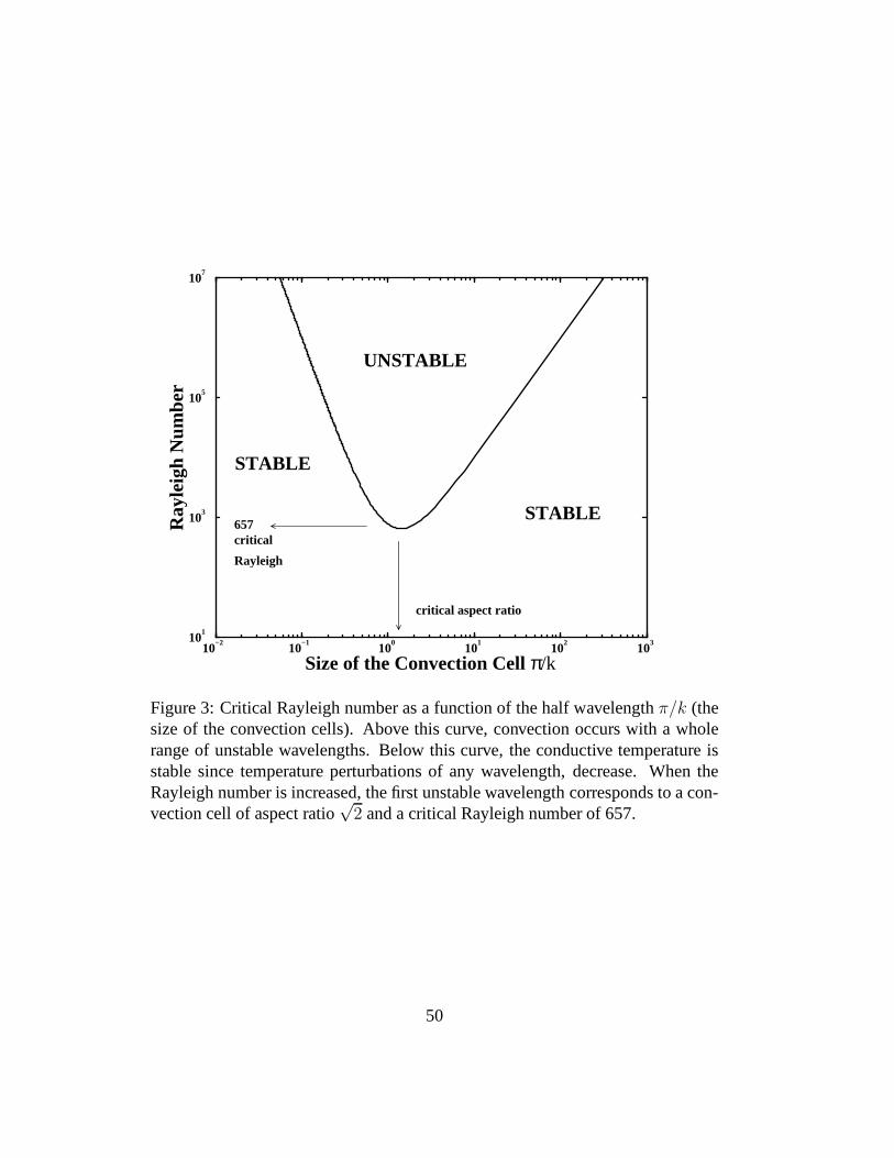
10−2

10−1

100

101

102

103

Size of the Convection Cell π/k

101

103

105

107

Ray

leig

h N

umbe

r

UNSTABLE

STABLE657

STABLE

critical

Rayleigh

critical aspect ratio

Figure 3: Critical Rayleigh number as a function of the half wavelengthπ/k (thesize of the convection cells). Above this curve, convectionoccurs with a wholerange of unstable wavelengths. Below this curve, the conductive temperature isstable since temperature perturbations of any wavelength,decrease. When theRayleigh number is increased, the first unstable wavelengthcorresponds to a con-vection cell of aspect ratio

√2 and a critical Rayleigh number of 657.

50

is orders of magnitude higher than critical and the mantle isin a chaotic state ofconvection.

Figure 4 shows a stationary convection pattern atRa = 105 and three snap-shots of numerical simulation of convection at higher Rayleigh number. The colorscale has been chosen differently in each panel to emphasizethe thermal structuresthat decrease in length scale withRa. This view is somewhat misleading since allthe thermal anomalies become confined in a top cold boundary layer and in a hotbottom one at large Rayleigh numbers. Most of the interior ofthe cell becomesjust isothermal (or adiabatic when anelastic equations areused). The various tran-sitions of convection as the Rayleigh number increases willbe discussed in otherchapters of this Treatise (see e.g., Chapter 4).

5 Introduction to physics of multicomponent and mul-tiphase flows

The mantle is not a simple homogeneous material. It is made ofgrains of variablebulk composition and mineralogy and contains fluids, magma and gases. Dis-cussion of multicomponent and multiphase flows could deal with solids, liquidsor gases, include compressibility or not, and consider elastic, viscous or morecomplex rheology. For each combination of these characteristics a geophysicalapplication is possible. Here we will restrict the presentation to viscous creepmodels (i.e., without inertia), where the various components are treated with con-tinuous variables (i.e., each component is implicitly present everywhere). We donot consider approaches where the various components are separated by movingand deformable interfaces. Our presentation excludes cases where the problemis to match properties at macroscopic interfaces between regions of different buthomogeneous compositions.

We will focus on two cases. First, when all the components areperfectly mixedin variable proportions. This corresponds to the classicalchemical approach ofmultiple components in a solution. This will provide some tools to understandmantle phase transitions and the physics of chemical diffusion and mixing. Wewill be rather formal and refer the applications and illustrations to other chaptersof this Treatise (e.g., Chapter 11 and Chapter 12). Our goal is to explain why andwhen the advection diffusion equation can be used in mantle dynamics. The irre-versible thermodynamics of multicomponent flows is discussed in various classi-cal books (e.g.,Haase, 1990;de Groot and Mazur, 1984). However as usual withgeophysical flows, the mantle has many simplifications and a few complexitiesthat are not necessarily well documented in these classicaltextbooks.

The second case will be for two phase flows in which the two phases are sepa-

51

Figure 4: Convection patterns of a fluid heated from below at Rayleigh number105, 106, 107, 108. The temperature color bars range from 0 (top boundary) to 1(bottom boundary). The Boussinesq approximation was used (numerical simula-tions by F. Dubuffet). The increase in Rayleigh number corresponds to a decreaseof the boundary layer thicknesses and the width of plumes. Only in the case of thelowest Rayleigh number (top left) is the convection stationary with cells of aspectratio ∼

√2 as predicted by marginal stability. For higher Rayleigh number, the

patterns are highly time-dependent.

52

rated by physical interfaces which are highly convolved andwith spatial character-istics much smaller than the typical size of geodynamic models. This is typicallythe case where magma can percolate through a compacting matrix. This approachwas used to model melt extraction and core-mantle interaction (McKenzie, 1984;Scott and Stevenson, 1984). Magma migration has also been treated in a largenumber of publications where solid and magma are consdered as separated (e.g.,in studies of dike propagation through hydraulic fracturing), or where fusion isparameterized in some way. We do not discuss these approaches.

5.1 Fluid dynamics of multicomponent flows in solution

5.1.1 Mass conservation in a multicomponent solution

If we want to study the evolution of major or trace element concentration in theconvecting mantle, we can consider the mantle, instead of a homogeneous fluid, asa solution of various componentsi in volumetric proportionsφi (with

∑

i φi = 1)having the densitiesρi and velocitiesvi (and later, thermal expansivitiesαi, heatcapacitiesCi

p...).Using a mass balance very similar to what we had discussed fora homoge-

neous fluid, we obtain a mass conservation equation of the form

∂(φiρi)

∂t+ ∇ · (φiρivi) = Γi, (143)

whereΓi is the rate of mass production of componenti. This rate of mass produc-tion is zero if no reactions produce the componenti.

In the fluid, the average density is

ρ =∑

φiρi, (144)

and various average velocities can be defined (weighted by the mass, the volume,the number of moles... of each componenti). In this section, we introduce thebarycentric velocity,vb (velocity of the center of mass), defined by

vb =

∑

φiρivi

ρ. (145)

The average mass conservation can be obtained by summing theequations ofcomponent conservation (143),

∂ρ

∂t+ ∇ · (ρvb) = 0, (146)

since the sum of the rates of mass production is zero∑

i

Γi = 0. (147)

53

In equation (143), instead of the various component velocitiesvi, we can intro-duce the barycentric velocityvb and the diffusive flux of the componenti withrespect to this average flow,

∂(φiρi)

∂t+ ∇ · (φiρivb) = −∇Ji + Γi, (148)

where we define the diffusive flux,Ji, by

Ji = φiρi(vi − vb). (149)

By definition of the barycentric velocity (145), the sum of the diffusive flows justcancels out,

∑

i

Ji = 0. (150)

A diffusive transport is nothing else than an advective transfer with respect to theaverage barycentric velocity. We will show later in simple cases, that the diffusivetransports are driven by concentration gradients.

If we introduce the mass fractionCi = φiρi/ρ (in kg of i per kg of mixture),we can easily show from (146) and (148) that

ρDCi

Dt= −∇Ji + Γi, (151)

where the Lagrangian derivative is defined with the barycentric velocity,

D

Dt=

∂

∂t+ vb · ∇. (152)

5.1.2 Momentum and energy in a multicomponent solution

In our multicomponent solution, all constituents are present at each point and theyare all locally submitted to the same pressure and stresses.We assume that theviscous stress is simply related tovb and we neglect inertia as appropriate for themantle. Newton’s second law (here, simply the balance of forces) can be appliedto the barycenter and implies

∇ · τ − ∇P + ρg = 0, (153)

where the only force is due to the (constant) gravity. The momentum equationthus remains identical to that of a fluid with uniform composition and withoutinertia (16).

Since there is only one momentum equation fori components thei − 1 othervelocity equations will be found by using the constraints ofthe laws of thermody-namics and in particular the positivity of the entropy source. To derive the energy

54

conservation, we perform the standard balance to account for all the energy ex-changes in a volumeΩ and across its surfaceΣ. Instead of the one componentequation (28), we have to sum up various contributions and weget

∑

i

∂(φiρiUi)

∂t= − ∇ ·

(

∑

i

φiρiUivi + P∑

i

φivi + q − τ · vb

)

+ g ·∑

i

φiρivi + ρH.(154)

In this expression, we recognize the temporal changes in energy (Ui is the compo-nent internal energy per unit mass, the kinetic energies areneglected), the energyadvection, the pressure work, the thermal diffusion, the viscous stress work, thegravity work and the radioactivity production (ρH =

∑

φiρiHi). The variousφi

come from the fact that each componenti is present in proportionφi, in the vol-umeΩ and on its surfaceΣ. We assume that thermal diffusion acts equally foreach component and that the surface work of the stress tensoris only related tothe barycentric velocity.

Using the definition of the barycentric velocity (145), of the diffusive fluxes,(149), of the momentum conservation, (153), and using

∑

i φi = 1, the energyexpression can be simplified to

∑

i

φiρiDHi

Dt= −∇ ·q−

∑

i

Ji ·∇Hi +DP

Dt−∑

i

ΓiHi +τ : ∇vb + ρH, (155)

whereHi are the component enthalpies

Hi = Ui +P

ρi

. (156)

The enthalpy variation for each componenti can be expressed as a function ofthe state variablesP andT . FromdHi = δQi + VidP and the expression of theexchanged heat (29), we can write

ρiDHi

Dt= ρiC

ip

DT

Dt+ (1 − αiT )

DP

Dt, (157)

Finally, the expression for the temperature evolution is

ρCpDT

Dt= −∇ ·q−

∑

i

Ji ·∇Hi + αTDP

Dt−∑

i

ΓiHi +τ : ∇vb + ρH, (158)

where the average heat capacity and thermal expansivity areCp =∑

i φiρiCip/ρ

andα =∑

i φiαi.Compared to the homogeneous case (36), two new heat source terms are

present, the enthalpy exchange through chemical reactions,∑

i ΓiHi, and the en-thalpy redistribution by component diffusion,

∑

i Ji · ∇Hi.

55

5.1.3 Entropy conservation in a multicomponent solution

Entropy conservation is essential for deriving the expressions of the diffusivefluxes. The general expression of entropy conservation (7) is

∑

i

∂(φiρiSi)

∂t= −∇ · JS +HS , (159)

whereJS andHS are the yet unknown entropy flux and source. The entropy of thevarious components take into account their specific entropies but also their con-figurational entropies or mixing entropies due to the dispersion of the componenti in the solution. Introducing the barycentric velocities and the diffusive fluxes,this equation can be recast as

∑

i

φiρiDSi

Dt= ∇·

(

∑

i

φiρiSivb +∑

i

SiJi − JS

)

+HS−SiΓi−Ji·∇Si. (160)

However a second expression of the entropy conservation canbe obtained fromthe enthalpy conservation, (155), usingdHi = TdSi + VidP which, in our casecan be expressed as

ρiDHi

Dt= ρiT

DSi

Dt+DP

Dt, (161)

we derive∑

i

φiρiTDSi

Dt= −∇ · q −

∑

i

Ji · ∇Hi −∑

i

ΓiHi + τ : ∇vb + ρH. (162)

A comparison of the two expressions for the entropy conservation, (160) and (162)allows us to identify the total entropy flux

JS =q

T+ vb

∑

i

φiρiSi +∑

i

SiJi, (163)

and the entropy sources

THS = −(q

T+∑

i

SiJi) ·∇T −∑

i

Ji ·∇µi −∑

i

Γiµi +τ : ∇vb + ρH. (164)

where we introduced the chemical potentialsµi = Hi − TSi. The total entropyflux, (163), is related to thermal diffusion and to advectionand chemical diffusionof component entropies.

In (164), the two gradients of chemical potential and temperature are not in-dependent as the chemical potential gradients implicitly include the temperaturegradient, so that alternative expressions can be found. Forexample, using

∇µi = T∇µi

T+ µi

∇T

T, (165)

56

andµi = Hi − TSi, the entropy source (164) can be written as

THS = −(q+∑

i

HiJi)∇T

T−T

∑

i

Ji ·∇µi

T−∑

i

Γiµi +τ : ∇vb + ρH. (166)

We can also introduce the gradient ofµ at constant temperature∇Tµ as

∇Tµi = ∇µi + Si∇T , (167)

which leads to

THS = − 1

Tq · ∇T −

∑

i

Ji · ∇Tµi −∑

i

Γiµi + τ : ∇vb + ρH. (168)

This last equation has the advantage of separating the temperature contribution,∇T , from the compositional contribution,∇Tµi (∇Tµi varies mostly with com-position as composition can change over very short distances, however this termis also related to pressure variations).

5.1.4 Advection-diffusion equation and reaction rates

Among the entropy sources, only terms involving similar tensorial ranks can becoupled in an isotropic medium, according to Curie’s principle. The positivity ofthe entropy production imposes three conditions, couplingtensors, vectors, andscalars.

τ : ∇vb ≥ 0, − q · ∇T

T−∑

i

Ji · ∇Tµi ≥ 0 −∑

i

Γiµi ≥ 0. (169)

The first term relates tensors and we have already discussed its implications forthe rheology in section 3.2.

The second term relates vectors and we assume, in agreement with the generalprinciple of non-equilibrium thermodynamics (de Groot and Mazur, 1984), thata matrix a phenomenological matrixM relates the thermodynamic fluxesJ =J1...Ji...q to the thermodynamic forcesX = −∇Tµ1...−∇Tµi...− ∇T/T

J1

J2

...q

= −

m11 m12 ... m1q

m21 m22 ... m2q

... ... ... ...mq1 mq2 ... mqq

∇Tµ1

∇Tµ2

...∇T/T

(170)

This linear relationship implies that the term of vectorialrank (with upperscriptv), in the entropy source,TH(v)

S appears as

TH(v)S = XtMX = XtM +M t

2X. (171)

57

According to the second law of thermodynamics, the symmetric part of the matrixM , (M + M t)/2 must be positive definite, i.e., the right hand side of equation(171) must be positive for any vectorsX.

Thermodynamic equilibrium is always dynamic on a microscopic scale. Tomaintain equilibrium, a process and its reverse must occur at the same microscopicrate. A consequence, known as the Onsager reciprocal relations, is the existenceof symmetry or antisymmetry betweenmij andmji (Onsager, 1903-1976). Ageneral discussion can be found in e.g.,de Groot and Mazur(1984) orWoods(1975). When the forces are even functions of the velocitiesand in the absence ofmagnetic field, the matrixM must be symmetric. As∇T/T, and∇Tµi are evenfunctions, as independent of the velocities,mij = mji.

In the general case, the transport of heat by concentration gradients (Dufoureffect, (Dufour, 1832-1892)) or the transport of concentration by temperature gra-dients (Soret effect, (Soret, 1827-1890)) are possible. Inmany situations thesecross-effects are small and we will assume that the matrixM does not couplethermal and compositional effects (the last row and column of M are zero exceptfor mqq/T = k, the thermal conductivity).

Even without coupling between thermal and compositional effects, chemicaldiffusion in a multicomponent system remains difficult to discuss in the most gen-eral case (the definite positivity of a symmetrici by i matrix is not a very strongconstraint). We therefore restrict our study to a simple two-component systemwhere

(

J1

J2

)

= −(

m11 m12

m21 m22

)(

∇Tµ1

∇Tµ2

)

(172)

For such a simple case, the sum of the flux must cancel, see (150), and since theOnsager relations impose the symmetry of the matrix, the coefficientsmij mustverify

m11 +m21 = m12 +m22 = m12 −m21 = 0. (173)

Only one coefficient, for examplem11 can be freely chosen, the fluxes can bewritten

J1 = m11∇T (µ2 − µ1), (174)

J2 = m11∇T (µ1 − µ2), (175)

and the second law requiresm11 > 0. If the component 1 is in small quantity (thesolute) and the component 2 is in large quantity (the solvent, with µ2 = 0), wecan easily track the evolution of solute concentrationC1. Its chemical diffusionflux is J1 = −m11∇Tµ1 and according to (151), its concentration satisfies

ρ(∂C

∂t+ vb · ∇C) = ∇ · (m∇Tµ) + Γ, (176)

where the subscripts1 have been omitted.

58

For a solute the chemical potential is a standard chemical potentialµ0 plus amixing term expressing the entropy gain (configuration entropy associated withthe increased disorder) made by dispersing the solute into the solvent, of the formRT log a(C) (for crystalline solids, the activitya(C) of the mixing term can becomplex since it depends on the number and multiplicity of crystallographic sites(Spear, 1993), but we just need to know that it is related toC). In a domain wherethe average density remains uniform, the advection-diffusion equation is obtained

∂C

∂t+ vb · ∇C = ∇ · (D∇C) + Γ (177)

with a diffusion coefficientD = m/ρ(∂µ/∂C), most likelyT -dependent. Thenegative linear relationship between chemical diffusion and concentration gradi-ent is called the first Fick’s law (Fick, 1829-1901).

When a component is present in two domains separated by a compositional in-terface, its standard chemical potentialµ0 is generally discontinuous. In this casethe gradient of the chemical potential at constantT , ∇Tµ is a mathematical dis-tribution that contains a term∇Tµ0, infinite on the compositional interface. Thisdiscontinuity drives an infinitely fast diffusion of the solute component across theinterface until the equilibrium[µ] = [µ0 + RT log a(C)] = 0. The concentrationratio ofC (or partition coefficient ofC), must therefore verify

a(C)+

a(C)−= exp (−µ

+0 − µ−

0

RT), (178)

where[ ]+ and[ ]− denote the values on the two sides of the discontinuity. Thisequation corresponds to the general rule of chemical equilibria.

The last entropy source in (169) relates two scalars (production rates andchemical potentials). In a mixture ofi components involvingk stable atomicspecies, the conservation of these atomic species implies that onlyr = i − k lin-early independent reactions exist. Letnj

i be the stoichiometric coefficient of thecomponenti in thejth = (1...r) chemical reaction with reaction rate,Γj . We canexpressΓi as

Γi =∑

j=1...r

njiΓj , (179)

and the second law imposes

−∑

j=1...r

Γj

∑

i

njiµi ≥ 0, (180)

The positivity of the entropy source is satisfied if the kinetic rates of thejth =1...r chemical reaction are proportional to the their chemical affinities, ∆Gj =∑

i njiµi, with positive reaction rate factorsRj

Γj = −Rj∆Gj . (181)

59

Chemical reaction rates are very rarely simply proportional to the affinities and theRj are likely some complex, but positive, functions ofP , T and concentrationsCi. In the case of exact thermodynamic equilibrium,

∑

i njiµi = 0, the second law

is of course satisfied.In the same way as we defined the affinity∆Gj of the reactionj, we can

define its enthalpy∆Hj =∑

i njiHi. The enthalpy exchange term of the energy

equation (158),∑

i ΓiHi can also be written∑

j Γj∆Hj , products of the reactionrates by the reaction enthalpies. Various phase changes take place in the mantle,most notably at 410 and 660 km depth. Their effects on mantle convection havebeen studied by various authors and will be discussed in section 6.6.

5.1.5 Conservation properties of the advection-diffusionequation

We now make the hypothesis that the evolution of concentration of a solute inthe convective fluid is controlled by the advection-diffusion equation (177), andthat this solute is not involved in any chemical reaction,Γ = 0. For simplicity,we assume that the barycentric flow is incompressible (C can therefore be a con-centration per unit volume or per unit mass) and the diffusion coefficientD is aconstant. The fluid and the solute cannot escape the domainΩ; the normal veloc-ity and normal diffusive flux are thus zero on the boundaries of the domain, i.e.,v · n = 0 and∇C · n = 0 on the surfaceΣ with normal vectorn.

First, it is obvious that when integrated over the total domain Ω and with thedivergence theorem, the advection diffusion equation (177) implies

d

dt

∫

ΩC dV = −

∫

Σ(Cv −D∇C) · dS = 0. (182)

The initial heterogeneity does not disappear, it is just redistributed through time.To understand how the heterogeneity is redistributed we canexpress the evo-

lution of the concentration variance. Multiplying (177) by2C, we get after somealgebra

∂C2

∂t+ ∇ · (vbC

2) = D∇2C2 − 2D|∇C|2. (183)

This expression when integrated over the closed volumeΩ implies that

d

dt

∫

ΩC2 dV = −2D

∫

Ω|∇C|2 dV . (184)

Since the right side is always negative, the variance must continuously decreaseuntil |∇C| = 0 which corresponds to a state of complete homogenization.

The concept of mixing is associated with the idea that the concentration vari-ance decreases with time. Since the average mixing rate is proportional to thediffusionD, (184), we note however, that a non-diffusive flow does not mix at

60

Figure 5: An initial heterogeneity (top) is introduced att = 0 into a time-dependent convection cell. Without diffusion,D = 0, (bottom left), the het-erogeneity is stirred by convection and then stretched on the form of thin ribbons.However the variance of the heterogeneity concentration remains constant. It isonly with diffusion,D 6= 0, (bottom right), that a real mixing occurs with a de-crease of the heterogeneity variance.

all. A diffusive flow just stirs the heterogeneities. In other terms, if the initialconcentration is eitherC = 1 orC = 0, a perfect mixing is achieved after a timetif the concentration is everywhereC = C, the average concentration. When thereis no diffusion, the initial heterogeneity is stirred and stretched, but the local con-centrations remain, for all time, eitherC = 1 orC = 0, but never an intermediatevalue (see Figure 5)

In the case of the Earth’s mantle, the solid state diffusion coefficients are allvery low (D = 10−19 m2 s−1 for uranium,D = 10−13 m2 s−1 for helium (see Table2)) and many studies have totally neglected chemical diffusion. We see, at facevalue, that these models are not really mixing, only stirring the heterogeneities.Without diffusion a chemical heterogeneity (e.g., a piece of subducted oceaniccrust) will forever remain the same petrological heterogeneity, only its shape willchange.

Since the mixing rate is related to the compositional gradient (184) we shoulddiscuss the evolution of this gradient. We multiply (177) bythe operator2∇C ·∇to obtain

∂|∇C|2∂t

+ ∇ · (vb|∇C|2) + 2∇C · ǫ · ∇C = 2D(

∇ · (∇2C∇C − (∇2C)2)

,

(185)

61

which can be integrated as

d

dt

∫

Ω|∇C|2 dV = −2

∫

Ω∇C · ǫ · ∇C dV − 2D

∫

Ω(∇2C)2 dV . (186)

The rate of gradient production is related to the flow properties through the strainrate tensorǫ and to the diffusion. The diffusion term is negative and decreases thesharpness of compositional gradients.

The term related to the flow properties through the strain tensor (first term ofthe right side of (186)), could in principle be either positive or negative. Howeveras time evolves, this term must become positive. The strain rate tensor has locallythree principal axes and three principal strain rates, the sum of them being zerosince the flow is incompressible. The stretched heterogeneities becomes elongatedalong the direction of the maximum principal strain rate andthe concentrationgradients reorient themselves along the minimum, and negative, principal strainrate. The term under the first integral on the right side of (186) is thus of orderof −ǫmin|∇C|2 (ǫmin is the local, negative eigenvalue of the strain rate tensor).Stirring is thus the source of production of concentration gradient.

We can now understand the interplay between advection and diffusion. Evenwhen the diffusion coefficientD is vanishingly small in (186), the stirring of theflow by convection will enhanced the concentration gradients until the average dif-fusion term, proportional to the concentration gradients,will become large enough(see (184)), for a rapid decrease of the concentration variance. We illustrate thisbehavior in the next two paragraphs by choosing a simple expression for the strainrate and computing the evolution of concentration through time.

5.1.6 Laminar and turbulent stirring

The efficiency of mixing, mostly controlled by stirring, is therefore related tothe ability of the flow to rapidly reduce the thickness of heterogeneities (Olsonet al., 1984). In this section we set aside diffusion and discuss a little bit more thestirring properties of a flow. Let us consider a vertical piece of heterogeneity ofwidth 2d0, height2L (L << d0) in a simple shear flow (or Couette flow, (Couette,1858-1943))ux = ǫz. Its top and bottom ends are at(0, L0), (0,−L0) and theywill be advected to(ǫtL0, L0), (−ǫtL0,−L0) after a timet. As the heterogeneitylength increases as2L0(1 + ǫ2t2), mass conservation implies that its half widthd(t) decreases as

d(t) =d0√

1 + ǫ2t2. (187)

Such flows, in which heterogeneities are stretched at rate∼ 1/t, are called flowswith laminar stirring. They are not very efficient in enhancing the diffusion be-

62

cause they do not increase the concentration gradients, typically of order1/d(t),fast enough.

On the contrary, in a pure shear flow,uz = zǫ, the length of the heterogeneitywould increase asL = L0 exp(ǫt) and its width would shrink as

d(t) = d0 exp(−ǫt). (188)

Such a flow is called flow with turbulent stirring. This usual vocabulary is verypoorly chosen because turbulent stirring can occur in a creeping flow withRe = 0.Mantle convection is not turbulent but it generates turbulent stirring.

Chaotic mixing flows have globally turbulent stirring properties and the qual-itative idea that highly time-dependent convection with high Ra number mixesmore efficiently than low Ra number convection is often true (Schmalzl et al.,1996). However steady 3D flows can also induce turbulent mixing. This surpris-ing phenomenon called Lagrangian chaos is well illustratedfor some theoreticalflows (Dombre et al., 1986) and for various simple flows (Ottino, 1989;Toussaintet al., 2000). For example, in a steady flow under an oceanic ridge offset by atransform fault, the mixing is turbulent (Ferrachat and Ricard, 1998).

5.1.7 Diffusion in Lagrangian coordinates

In section 5.1.5 we discussed the mixing properties from an Eulerian viewpoint.We can also understand the interplay between diffusion and stretching (stirring) byadopting a Lagrangian viewpoint (Kellogg and Turcotte, 1987;Ricard and Coltice,2004), i.e., by solving the advection-diffusion equationsin a coordinate frame thatfollows the deformation.

Let us consider a strip of thickness2l0 with an initial concentrationC0 em-bedded in a infinite matrix of concentrationC∞. In the absence of motion, thesolution of the advection-diffusion equation (177) can be expressed using the er-ror function and the time dependent concentrationC(x, t) is given by

C(x, t) − C∞

C0 − C∞

=1

2

[

erf

(

l0 − x

2√Dt

)

+ erf

(

l0 + x

2√Dt

)

,

]

(189)

wherex is a coordinate perpendicular to the strip and is zero at its center.The concentration at the center of the strip(x = 0) is

C(0, t) − C∞

C0 − C∞

= erf

(

l0

2√Dt

)

, (190)

and the concentration decreases by a factor of about 2 in the diffusive time

t0 ∼l20D. (191)

63

(erf(1/2) is not far from1/2). The time needed to homogenize a 7 km thick pieceof oceanic crust introduced into a motionless mantle is extremely long (see Table2). In a motionless mantle, even the relatively mobile helium would be frozensince the Earth formed since it would only have migrated around 50 cm.

However, this idea of a√t diffusion is totally wrong since the flow stirs the

heterogeneity and increases the quantity of compositionalgradients (186) whichin turn accelerates the mixing process (184). Assuming thatthe problem remainstwo-dimensional enough so that diffusion only occurs perpendicular to the de-forming heterogeneity, letl(t) be the thickness of the strip containing a chemicalheterogeneity. The velocity perpendicular to the strip would locally be at firstorder

vx =x

l(t)

d

dtl(t), (192)

(each side of the stripe, atx = ±l(t) moves at±dl(t)/dt).We can choose as a new space variablex = xl0/l(t), in such a way that

the Lagrangian coordinatex will vary between the fixed values -l0 and l0. Thediffusion equation becomes

(

∂C

∂t

)

x

= D

(

l0l(t)

)2∂2C

∂x2, (193)

where the partial time derivative is now computed at constant x. We see that theadvection diffusion equation has been turned into a pure diffusive equation wherethe diffusivityD has been replaced byD (l0/l(t))

2. This equivalent diffusivity islarger than D and increases with time asl(t) decreases.

To solve analytically equation (193) it is appropriate to rescale the time vari-able by definingt = F (t) with

F (t) =∫ t

0(l0/l(u))

2 du, (194)

and the resulting advection-diffusion equation in Lagrangian coordinates becomesthe simple diffusion equation with constant diffusivity. Its solution is given by(189) wheret andx are replaced byt andx. For example, the concentration at thecenter of the deformable strip varies like

C(0, t) − C∞

C0 − C∞

= erf

l0

2√

DF (t)

, (195)

and the concentration diminishes in amplitude by a factor of2 after a timet thatsatisfies

F (t) ∼ l20D. (196)

64

Table 2: Homogenization times for helium and uranium assuming an heterogene-ity of initial thickness2l0 = 7 km and a strain rate of5 × 10−16 s−1.

Uranium HeliumD m2 s−1 10−19 10−13

t0 ma 3.88 × 1013 3.88 × 107

tL ma 3.60 × 105 3.60 × 103

tT ma 1920 1490

To perform a numerical application let us consider that the flow is either a simpleshear (187), or a pure shear deformation, (188). ComputingF (t) from equation(194) is easy and, assumingǫt >> 1, we get from (196), the homogenizationtimes

tL ∼ 31/3l2/30

ǫ2/3D1/3, (197)

and

tT ∼ 1

2ǫlog

2l20ǫ

D, (198)

respectively. For the same oceanic crust of initial thickness 7 km, we get homoge-nization times of about 1.49 byr for He and 1.92 byr for U if we use the pure shearmechanism and assume rather arbitrary thatǫ = 5 × 10−16 s−1 (this correspondsto a typical plate velocity of 7 cm yr−1 over a plate length of 5000 km). AlthoughHe and U have diffusion coefficients 6 orders of magnitude apart, their residencetimes in a piece of subducted oceanic crust may be comparable.

The use of tracers to simulate the evolution of chemical properties in the man-tle, is our best method since solid state diffusion is too slow to be efficiently ac-counted for in a numerical simulations (e.g.,van Keken et al., 2002;Tackley andXie, 2002). However, by using tracers, we do not necessarily take into account thatsome of them may represent points that have been stretched somuch that their ini-tial concentration anomalies have diffused totally into the background. In otherwords, even if diffusion seems negligible, diffusion will erase all heterogeneitiesafter a finite time mostly controlled by the stirring properties of the flow.

5.2 Fluid dynamics of two phase flows

Up to now, in all of section 5.1, all components were mixed in asingle phase.However, another important geophysical application occurs when the multicom-ponents belong to different phases. This case can be illustrated with the dynamicsof partial melt in a deformable compacting matrix. Partial melts are obviously

65

present under ridges and hotspots, but they may also be present in the middleand deep mantle (Williams and Garnero, 1996;Bercovici and Karato, 2003) andthey were certainly more frequent when the Earth was younger. We discuss thesituation where two phases, fluid and matrix, each having thesame composition,can interact. In contrast to section 5.1, where the proportion and velocity of eachcomponent in solution was defined everywhere at a microscopic level, in a partialmelt aggregate, the local velocity at a microscopic level iseither the velocity of amatrix grain,vm, or the interstitial velocity of the melt,vf .

We assume that the two phases are individually homogeneous,incompressibleand with densitiesρf andρm. They have Newtonian rheologies with viscositiesµf andµm. They are isotropically mixed and connected. Their volume fractionsareφ (the porosity) and1 − φ. The rate of magma melting or freezing is∆Γ (inkg m−3 s−1). Although the two phases have very different physical properties wewill require the equations to be material invariant until weneed to use numericalvalues. This means that swappingf andm, φ and1−φ, ∆Γ and−∆Γ, must leavethe equations unchanged. This rule is both a physical requirement and a strongguidance in establishing the general equations.

We make the hypothesis that there is a mesoscopic size of volumeδV whichincludes enough grains and interstitial fluid that averagedand continuous quanti-ties can be defined. Classical fluid dynamics also has its implicit averaging vol-umeδV that must contain enough atoms that quantum effects are negligible, butwhat is needed here is a much larger volume. This averaging approach remainsmeaningful because the geophysical macroscopic phenomenon that we want tounderstand (say, melting under ridges) has characteristicsizes large compared tothose of the averaging volume (say, a few cm3).

To do the averaging, we define at microscopic level a functionθ that takes thevalue 1 in the interstitial fluid and the value 0 in the matrix grain. Mathematically,this function is rather a distribution and it has a very convolved topology. Fromit, we can define first, the porosity (volume fraction of fluid)φ, then, the fluid andmatrix averaged velocities,vf andvm by

φ =1

δV

∫

δVθ dV , (199)

φvf =1

δV

∫

δVθvf dV , (1 − φ)vm =

1

δV

∫

δV(1 − θ)vm dV . (200)

5.2.1 Mass conservation for matrix and fluid

Having defined the average quantities, the derivation of thetwo mass conservationequations is fairly standard (McKenzie, 1984;Bercovici et al., 2001a). They are

∂φ

∂t+ ∇ · [φvf ] =

∆Γ

ρf, (201)

66

−∂φ∂t

+ ∇ · [(1 − φ)vm] = −∆Γ

ρm. (202)

We get the same equations as in (143) except that we refer toφ, 1 − φ, ∆Γ in-stead ofφ1, φ2 andΓ1. When averaged, the mass conservation equations of twoseparated phase takes the same form as the mass conservationequations of twocomponents in a solution.

We define an average and a difference quantity for any generalvariableq, by

q = φqf + (1 − φ)qm, ∆q = qm − qf . (203)

The velocityv is volume averaged and is different from the barycentric velocity(145),vb = (φρfvf + (1− φ)ρmvm)/ρ. By combining the fluid and matrix massconservation equations we get the total mass conservation equation

∂ρ

∂t+ ∇ · (ρvb) = 0, (204)

(as before, (146)), and the time rate of change in volume during melting

∇ · v = ∆Γ∆ρ

ρfρm. (205)

5.2.2 Momentum conservation of matrix and fluid

Total momentum conservation, i.e., the balance of the forces applied to the mix-ture is

∇ · τ − ∇P + ρg = 0. (206)

We have considered that the only force is due to gravity, although surface tensionbetween the two phases could also be introduced (Bercovici et al., 2001a). In thisequation,P , τ andρ are the average pressure, stress and density. The equation isnot surprising and looks identical to its counterpart for a multicomponent solution(153). However the average pressure and stresses,P = φPf + (1 − φ)Pm andτ = φτ f + (1 − φ)τm are now the sum of two separate contributions, fromtwo separate phases having most likely very different rheologies and differentpressures. Hypothesizing that the two phases may feel the same pressure doesnot rest on any physical justification and certainly cannot hold if surface tensionis present. We will show later that their pressure difference controls the rate ofporosity change.

We split the total momentum equation into two equations one for the fluid andone for the matrix

−∇[φPf ] + φρfg + ∇ · [φτ f ] + hf = 0, (207)

67

−∇[(1 − φ)Pm] + (1 − φ)ρmg + ∇ · [(1 − φ)τm] + hm = 0. (208)

wherehf andhm satisfyhf + hm = 0 and represent the interaction forces actingon the fluid and on the matrix, across the interfaces separating the two phases.Because of the complexities of the interfaces, these two interaction forces must beparametrized in some way.

The simplest contribution to the interfacial forces that preserves Galilean in-variance is a Darcy-like termc∆v = c(vm − vf ) (Drew and Segel, 1971) (Darcy,1803-1858). In the absence of gravity and when the pressuresare uniform andequal, no motion should occur even in the presence of non-uniform porosity. Inthis situation where∆v = τ f = τ m = 0 and whereP is uniform,P = Pf = Pm,the force balances are−P∇φ + hf = −P∇(1 − φ) + hm = 0. Therefore, theinterface forceshf andhm, must also include−P∇φ and−P∇(1 − φ) whenthe two pressures are equal. This ledBercovici and Ricard(2003) to write theinteraction terms

hf =c∆v + Pf∇φ+ ω∆P∇φ,

hm = − c∆v + Pm∇(1 − φ) + (1 − ω)∆P∇φ.(209)

These expressions verifyhf + hm = 0, are Galilean and material invariant andallow equilibrium of a mixture with non uniform porosity butuniform and equalpressures.

The interaction coefficientc is related to permeability which is itself a functionof porosity. A symmetrical form compatible with the usual Darcy term is (seeBercovici et al., 2001a)

c =µfµm

k0[µf(1 − φ)n−2 + µmφn−2], (210)

where the permeability of the formk0φn was used (usuallyn ∼ 2–3). Assuming

n = 2 andµm ≫ µf , the interaction coefficient becomes a constant,c = µf/k0.At microscopic level, the matrix-melt interfaces are not sharp discontinuities

but correspond to layers (called “selvage” layers) of disorganized atom distribu-tions. The coefficient0 < ω < 1 controls the partitioning of the pressure jump(and potentially of the surface tension) between the two phases (Bercovici andRicard, 2003) and represents the fraction of the volume-averaged surface forceexerted on the fluid phase. The exact value ofω is related to the microscopicbehavior of the two phases (molecular bond strengths and thickness of the inter-facial selvage layers) and measures the extent to which the microscopic interfacelayer is embedded in one phase more than the other. The only general physicalconstraints that we have are thatω must be zero when the fluid phase disappears(whenφ = 0) and when the fluid phase becomes unable to sustain stresses (when

68

µf = 0). A symmetrical form like

ω =φµf

φµf + (1 − φ)µm(211)

satisfies these conditions.To summarize, general expressions for the equations of fluidand matrix mo-

mentum conservation are (Bercovici and Ricard, 2003)

−φ[∇Pf − ρfg] + ∇ · [φτ f ] + c∆v + ω∆P∇φ = 0, (212)

−(1− φ)[∇Pm − ρmg] + ∇ · [(1− φ)τm]− c∆v + (1−ω)∆P∇φ = 0. (213)

The relationship between stress and velocities does not include an explicit bulkviscosity term (Bercovici et al., 2001a), and for each phasej the deviatoric stressis simply

τ j = µj

(

∇vj + [∇vj]t − 2

3∇ · vj I

)

, (214)

wherej stands forf orm. There is no difference between the expression of therheology for the isolated component and for the component inthe mixture.

5.2.3 Energy conservation for two-phase flows

In the case where surface energy and entropy exist on interfaces the conservationof energy deserves more care (Sramek et al., 2006). Otherwise the global conser-vation is straightforward and can be expressed by the following equation wherethe left side represents the temporal change of energy content in a fixed controlvolume and the right side represents the different contributions to this change,namely internal heat sources, loss of energy due to diffusion, advection of energy,and rate of work of both surface and body forces,

∂

∂t[φρfUf + (1 − φ)ρmUm]

= ρH − ∇ · q − ∇ · [φρfUfvf + (1 − φ)ρmUmvm]

+ ∇ · [−φPfvf − (1 − φ)Pmvm + φvf · τ f + (1 − φ)vm · τ m]

+ φvf · ρfg + (1 − φ)vm · ρmg.

(215)

The last equation is manipulated in the standard way using the mass and momen-tum equations. Because the two phases are incompressible, their internal energiesare simplydUf = CfdT anddUm = CmdT . After some algebra we get

φρfCfDfT

Dt+ (1 − φ)ρmCm

DmT

Dt

= −∇ · q − ∆PDωφ

Dt+ ∆H∆Γ + Ψ + ρH,

(216)

69

whereΨ is the rate of deformational work

Ψ = φ∇vf : τ f + (1 − φ)∇vm : τm + c(∆v)2. (217)

It contains the dissipation terms of each phase plus a term related to the frictionbetween the two phases. The fundamental derivatives are defined by

Dj

Dt=

∂

∂t+ vj · ∇ , (218)

wherevj is to be substituted with the appropriate velocityvf , vm or vω with

vω = ωvf + (1 − ω)vm, (219)

In contrast to section 5.1 it would not make much sense to try to keep the equa-tions in terms of an average velocity likevb plus some diffusion terms. Here thetwo components may have very different velocities and we have to define varioussubstantial derivatives.

Sinceω represents a partitioning of pressure jump, it is not surprising to findthe velocityvω (included inDω/Dt) in the work term related to this pressurejump. Associated with this partitioning factor, we can alsointroduce interfacevalues,qω, that we will use later. Any quantity∆q = qm − qf can also be written(qm−qω)−(qf −qω). When the property jump is embedded entirely in the matrix(ω = 0), there should be no jump within the fluid and we must haveqω = qf .Reciprocally, whenω = 1, we should haveqω = qm. This prompts to defineinterface values by

qω = (1 − ω)qf + ωqm. (220)

Notice by comparing the expressions of the interface velocity vω, (219), and in-terface value,qω (220), thatω swaps with1 − ω.

The right side of (216) contains two new expressions in addition to the usualterms (heat production, diffusion and deformational work). The first term includesthe changes in porosityDωφ/Dt times the difference in pressures between phases,∆P . The other term contains the difference in the specific enthalpies ∆H =Hm−Hf where the enthalpy of phasej is defined byHj = Uj +Pj/ρj. A similarterm was found for components reacting in a solution (155).

5.2.4 Phenomenological laws

Entropy conservation is needed to constrain the the pressure jump between phasesand the melting rate. Starting from entropy conservation

∂

∂t[φρfSf + (1 − φ)ρmSm] = −∇ · JS +HS , (221)

70

whereJS is the total entropy flux andHS is the internal entropy production, wecompare the energy and the entropy equations (216) and (221)taking into ac-count that, for each incompressible phase,dsj = CjdT/T = duj/T . After somealgebra, one gets

JS = φρfSfvf + (1 − φ)ρmSmvm +q

T, (222)

THS = − 1

Tq · ∇T − ∆P

Dωφ

Dt+ ∆µ∆Γ + Ψ + ρH, (223)

where we have introduced the difference in chemical potentials between the twophases

∆µ = ∆H− T∆S (224)

and∆S = Sm − Sf is the change in specific entropies.Following the standard procedure of non-equilibrium thermodynamics, we

chooseq = −k∇T and we assume that there is a linear relationship betweenthe two thermodynamic fluxes,Dωφ/Dt and∆Γ, and the two thermodynamicforces−∆P and∆µ since they have the same tensorial rank. We write

(

Dωφ/Dt∆Γ

)

=

(

m11 m12

m21 m22

)(

−∆P∆µ

)

(225)

The matrix of phenomenological coefficientsmij is positive definite and symmet-rical by Onsager’s theorem,m12 = m21, as the two thermodynamic forces (−∆Pand∆µ) are even in velocity. For a 2x2 matrix, it is rather simple toshow that thepositivity implies,m22 > 0, m11 > 0 andm11m22 − m2

12 > 0 (positivity of thedeterminant).

The form of the phenomenological coefficientsmij can be constrained throughthought experiments. First using mass conservations (201)and (202) and the def-initions ofvω andρω, (219) and (220), we can combine equations (225) to get

∆P = − m22

m11m22 −m212

[

(1 − ω)(1 − φ)∇ · vm − ωφ∇ · vf +

(

ρω

ρfρm− m12

m22

)

∆Γ

]

.(226)

In the limiting case where the two phases have the same density ρf = ρm = ρω,melting can occur with no motion,vm = vf = 0, (226) should therefore predictthe equality of pressure between phases,∆P = 0. In this case we must choosem12/m22 = 1/ρf = 1/ρm. Let us consider now a situation of homogeneousisotropic melting where the melt has such a low viscosity that it cannot sustainviscous stresses and cannot interact with the solid by Darcyterms. For such an

71

inviscid melt,ω = 0, ρω = ρf andvω = vm. In this case, since the melt canescape instantaneously, the matrix should not dilate,∇ · vm = 0, and thus thetwo pressures should also be the same,∆P = 0. In this situation all the terms inequation (226) are 0 except for the term proportional to∆Γ. This suggests in thegeneral case, that

m12

m22

=ρω

ρfρm

. (227)

Using this condition and introducing two positive coefficients,ζ = m22/(m11m22−m2

12), andR = m22, we can recast equations (225) as

∆P = −ζ[

Dωφ

Dt− ρω

ρfρm

∆Γ

]

, (228)

∆Γ = R[

∆µ− ρω

ρfρm∆P

]

(229)

The first equation establishes a general relation controlling the pressure dropbetween phases. The coefficientζ that links the pressure jump between the twophases to the porosity changes in excess of the melting rate,is in fact equiva-lent to a bulk viscosity as introduced in section 3.2 (see also the summary section5.2.5). The physical requirement that the two phase mixtureshould have the in-compressible properties of either the matrix or the fluid when φ = 0 or φ = 1imposes a porosity dependence toζ with limφ→0 ζ(φ) = limφ→1 ζ(φ) = +∞.Simple micromechanical models (e.g.,Nye, 1953;Bercovici et al., 2001a) allowus to evaluate the bulk viscosity as

ζ = K0(µf + µm)

φ(1 − φ). (230)

The dimensionless constantK0 accounts for grain/pore geometry and is ofO(1).A more general, but more hypothetical, interpretation of the entropy positivity

could argue that some deformational work,Ψ, might affect the pressure drop of(228). This hypothesis led to a damage theory developed in (Bercovici et al.,2001b;Ricard and Bercovici, 2003;Bercovici and Ricard, 2005). Here we assumethat the system remains close enough to mechanical equilibrium that damage doesnot occur.

The second equation (229) controls the kinetics of the melting/freezing and byconsequence, defines the equilibrium condition. In the caseof mechanical equi-librium, when there is no pressure drop between the two phases, the melting ratecancels when there is equality of the chemical potentials ofthe two single phases.In case of mechanical disequilibrium, (∆P 6= 0), the chemical equilibrium does

72

not occur when the two chemical potentials are equal. We define a new effectivechemical potential,

µ∗

i = Ui +P ω

ρi− TSi, (231)

wherei stands forf orm and write the kinetic equation (229),

∆Γ = R∆µ∗. (232)

Chemical equilibrium imposes the equality of the effectivepotentials on the inter-face, at the pressureP ω at which the phase change effectively occurs.

Using (228) and (229), we can show that the entropy production is indeedpositive and given by

THS = k1

T|∇T |2 +

∆P 2

ζ+

(∆µ∗)2

R + Ψ + ρH. (233)

Chemical relaxation and bulk compression are associated with dissipative terms.

5.2.5 Summary equations

For convenience we summarize the governing equations when the matrix is muchmore viscous than the fluid phase (µf ≪ µm) as typical for melting scenarios,which implies thatτ f = 0, ω = 0, ρω = ρf , P ω = Pf , andvω = vm.

The mass conservations equations are (201) and (202). The equation of con-servation of momentum for the fluid phase is

−φ∇[Pf + ρfgz] + c∆v = 0, (234)

(assumingz positive upward). This is a typical Darcy equilibrium withc =µfφ

2/k(φ), wherek is the permeability (often varying ask0φn with n = 2 or

3). The second momentum equation could be the matrix momentum (208) or acombined force-difference (or action-reaction) equation

−∇[(1 − φ)∆P ] + (1 − φ)∆ρg + ∇ · [(1 − φ)τm] − c∆v

φ= 0, (235)

where the deviatoric stress in the matrix is given by

τ m = µm

(

∇vm + [∇vm]T − 2

3∇ · vmI

)

. (236)

and the pressure jump between phases, (228), becomes

∆P = −ζ(1 − φ)∇ · vm, (237)

73

if an equivalent bulk viscosity is used, or

∆P = −K0µm∇ · vm

φ, (238)

from the micromechanical model, (230), ofBercovici et al.(2001a).The action-reaction equation (235) can also be written in a different way for

example by elimination of∆v taken from the Darcy equilibrium (234),

−∇Pf + ∇ · [(1 − φ)τ ∗

m] + ρg = 0, (239)

whereτ∗

m includes the∆P term and is defined by

τ∗

m = µm

(

∇vm + [∇vm]T − 2

3∇ · vmI

)

+ ζ(1− φ)∇ · vmI. (240)

This shows that if the pressure is defined everywhere as the fluid pressure, thenit is equivalent to use for the matrix a rheology, (see (91)),with a bulk viscosity(1 − φ)ζ ∼ ζ (McKenzie, 1984). This analogy only holds without surface tensionbetween phases.

The rate of melting is controlled by

∆Γ = R(

∆u+ Pf

(

1

ρm− 1

ρf

)

− T∆s

)

, (241)

and the energy equation is

ρfφCfDfT

Dt+ ρm(1 − φ)Cm

DmT

Dt− ∆H∆Γ =

ρH − ∇ · q +∆Γ2

R +K0µm1 − φ

φ(∇ · vm)2 + Ψ,

(242)

where we have assumed the relation (238).These equations have been used by many authors with various levels of ap-

proximation. The most benign have been to replace1−φ by 1. Most authors havealso considered the bulk viscosityζ as a porosity independent parameter, (e.g.,McKenzie, 1984;Scott and Stevenson, 1984;Richter and Mckenzie, 1984;Ribe,1985a,b;Scott and Stevenson, 1986, 1989;Stevenson, 1989;Kelemen et al., 1997;Choblet and Parmentier, 2001;Spiegelman et al., 2001;Spiegelman and Kelemen,2003;Katz et al., 2004). This overestimates the possibilities of matrix compactionat low porosity. Porosity dependent parameters have been explicitly accounted forin other papers (e.g.,Fowler, 1985;Connolly and Podladchikov, 1998;Schmeling,2000;Bercovici et al., 2001a;Ricard et al., 2001;Rabinowicz et al., 2002). Themelting rates are sometimes imposed instead of solving the energy equation (e.g.,

74

Turcotte and Morgan, 1992) or solved for assuming univariant transition (Fowler,1989;Sramek et al., 2006). Surface tension is added inRiley et al.(1990) and(Hier-Majumder et al., 2006). Similar equations have also been used to describethe interaction between iron and silicates near the CMB (Buffett et al., 2000), theformation of dendrites (Poirier, 1991) or the compaction of lava flows (Massolet al., 2001).

6 Specifics of Earth’s mantle convection

In this last section we discuss various aspects of large-scale mantle convection.We leave the problems of partial melting to Chapter 9 and Chapter 11 of thisTreatise. We are aware of the impossibility to be exhaustivebut most of the im-portant points are more deeply developed in other chapters of the Treatise (seealso the books bySchubert et al.(2001) andDavies(1999)).

6.1 A mantle without inertia

The most striking difference between mantle convection andmost other convec-tion experiments is that inertia is totally negligible. This is because the Prandltnumber is infinitly larger than the (already very large) Rayleigh number. Thisimplies than the mantle velocity field obeys

∇ · (ρv) = 0,

−∇P + ∇ · τ + δρg + ρδg = 0,

∇2ψ = 4πGδρ,

δg = −∇ψ,

(243)

in agreement with (125). In this set of equation we kept the self-gravitation termas appropriate at long wavelengths. If the internal loadsρ are knowns, the flow canbe computed independently of the temperature equation. This time-independentsystem has been used by many authors to try to infer the mantleproperties.

6.1.1 Dynamic models

The system of equation (243) can been solved analytically for a depth-dependentviscosity, when variables are expressed on the basis of spherical harmonics (seeHager and Clayton(1989) and also Chapter 5 and Chapter 8). Various possiblesurface observables (geoid height or gravity free air anomalies, velocity diver-gence, amplitude of deviatoric stress at the surface, surface dynamic topography,CMB topography...) can be expressed on the basis of spherical harmonics with

75

componentsOlm. Through (243), they are related to the spherical harmonicscom-ponents of the internal density variationsδρlm(r) by various degree-dependentGreen’s functions (Green, 1793-1841)

Olm =∫

GOl (r)δρlm(r) dr (244)

(see Chapter 5 for analytical details). The Green’s functionsGOl (r) can be com-

puted from the averaged density and viscosity profiles.Before seismic imaging gave us a proxy of the 3D density structure of the man-

tle, various theoretical attempts have tried to connect models of mantle convectionto plate velocities (Hager and Oconnell, 1979;Hager and O’Connell, 1981), tothe Earth gravity field (or to the geoid, proportional toψ), to the lithospheric stressregime or to the topography (Runcorn, 1964;Parsons and Daly, 1983;Lago andRabinowicz, 1984;Richards and Hager, 1984;Ricard et al., 1984).

An internal load of negative buoyancy induces a downwellingflow that de-flects the Earth’s surface, the CMB and any other internal compositional bound-aries, if they exist. The amount of deflection corresponds tothe usual isostaticrule for a load close to an interface: the weight of the induced topography equalsat first order the mass of the internal load. The total gravityanomaly resultingfrom a given internal load is affected by the mass anomalies associated with theflow-induced boundary deflections as well as by the load itself. Due to the de-flection of the Earth’s surface, the geoid perturbation induced by a dense sinkinganomaly is generally negative (e.g., free air gravity has a minimum above a denseload). However, when the mantle viscosity increases significantly with depth, by1-2 orders of magnitude, a mass anomaly close to the viscosity increase, inducesa larger CMB deformation and a lower surface deformation. The resulting gravityanomaly corresponds to a geoid high. The fact that cold subduction zones corre-spond to a relative geoid high suggests a factor≥ 30 viscosity increase around theupper-lower mantle interface (Lago and Rabinowicz, 1984;Hager et al., 1985).Shallow anomalies and anomalies near the CMB, being locallycompensated, donot contribute to the long-wavelength gravity field. The lithospheric stress field,like the geoid, is affected by mid-mantle density heterogeneities. The surface de-flection induced by a deep seated density anomaly decreases with the depth ofthis anomaly but even lower mantle loads should significantly affect the surfacetopography.

6.1.2 Mantle flow and post-glacial models

As soon as seismic tomography started to image the mantle structures, these seis-mic velocity anomalies have been used to further constrain the mantle viscosity.The fact that the geoid and seismic velocity anomalies are positively correlated

76

around the transition zone but negatively in the deep mantleheterogeneities sug-gests a viscosity larger than 10 but not too large (less than 100) otherwise the man-tle would be everywhere positively correlated with gravity(Hager et al., 1985;Hager and Clayton, 1989;King and Hager, 1994). The same modeling approach,assuming a proportionality between seismic velocity anomalies and density vari-ations, was also used to match the observed plate divergence(Forte and Peltier,1987), the plate velocities (Ricard and Vigny, 1989;Ricard et al., 1991) and thelithospheric stresses (Bai et al., 1992;Lithgow-Bertelloni and Guynn, 2004). Theinitial Boussinesq models were extended to account for compressibility (Forte andPeltier, 1991).

Joint inversions of gravity with postglacial rebound were also performed tofurther constrain the mantle viscosity profile. The viscosity increase required bysubduction was initially thought to be too large to reconcile with post glacialrebound (Peltier, 1996). The various approaches (time-dependent for the post-glacial models and time-independent for the geoid models) seem to have con-verged to a standard viscosity profile with a significant increase with depth (Mitro-vica and Forte, 1997). Whether this viscosity increase occurs across a disconti-nuity (at the upper-lower mantle interface, or deeper) or asa gradual increase isprobably beyond the resolution of these approaches.

Although these dynamic models explain the observed geoid, they require thepresence of a kilometric surface topography, induced by mantle convection andcalled dynamic topography (by opposition with the isostatic topography related tocrustal and lithospheric density variations). Its direct observation, from the Earth’stopography corrected from isostatic crustal contributions, is difficult and remainscontroversial (e.g.,Colin and Fleitout, 1990;Kido and Seno, 1994;Lestunff andRicard, 1995;Lithgow-Bertelloni and Silver, 1998).

6.1.3 Time dependent models

The thermal diffusion in the mantle is so slow that even over 100-200 myrs it canbe neglected in some long wavelength global models. The equations (243) canthus be solved by imposing the known paleo-plate velocitiesat the surface and ad-vect the mass anomalies with the flow without solving explicitly the energy equa-tion. This forced-convection approach has shown that the deep mantle structureis mostly inherited from the Cenozoic and Mesozoic plate motion (Richards andEngebretson, 1992;Lithgow-Bertelloni and Richards, 1998). From plate paleo-slab reconstructions only, a density models can be obtainedthat gives a strikingfit to the observed geoid and is in relative agreement with long-wavelength to-mography (Ricard et al., 1989). This approach was also used to study the hotspotfixity (Richards, 1991;Steinberger and O’Connell, 1998), the sea level changes(Lithgow-Bertelloni and Gurnis, 1997) or the polar wander of the Earth (Spada

77

-2900

-2610

-2320

-2030

-1740

-1450

-1160

-870

-580

-290

0

Dep

th z

5 10 15 20

degree l

-2900

-2610

-2320

-2030

-1740

-1450

-1160

-870

-580

-290

0

Dep

th z

5 10 15 20

degree l

-1.0 -0.5 -0.3-0.2-0.10.00.10.20.3 0.5 1.0

Correlation Tomography-Geoid

-5e-05 -2,5e-05 0 2,5e-05 5e-05

Greoid Green function

0,5

0,6

0,7

0,8

0,9

1

Nor

mal

ized

rad

ius

µlower

/µupper

=1

µlower

/µupper

=30

µlower

/µupper

=100

-1e-05 -5e-06 0 5e-06Geoid Green function

0,5

0,6

0,7

0,8

0,9

1

Nor

mal

ized

rad

ius

µlower

µupper

=1

µlower

/µupper

=30

µlower

/µupper

=100l=2 l=10

Figure 6: Correlations between gravity and the synthetic tomographic Smeanmodel (Becker and Boschi, 2002) as a function of degreel and normalized ra-dius (top). The seismic velocities, proxy of the density variations, are positivelycorrelated with gravity around the upper-lower mantle interface (warm colors) butnegatively correlated, near the surface and in the deep lower mantle (cold colors).Geoid Green functions for degree 2 (bottom left) and degree 10 (bottom right)and three possible viscosity increases between upper and lower mantle. The geoidGreen function for a uniform viscosity (dashed line) is everywhere negative andall the anomalies around the upper-lower mantle would induce a gravity signal op-posite to that observed. A too large viscosity increase (a factor 100 for the dottedlines) cannot explain the rather good negative correlationbetween lower mantleanomalies and the geoid at long wavelength. A moderate increase (a factor 30 forthe solid line) leads to the best fit as the sign of the Green functions is everywherethat of the observed density-gravity correlations. The different Green functionsare computed for an incompressible mantle, with a lithosphere, 10 times moreviscous than the upper mantle.

78

et al., 1992;Richards et al., 1997).

6.2 A mantle with internal heating

When the top and bottom boundary conditions are the same (i.e., both free-slip orboth no-slip), purely basally heated convection in a Cartesian box leads to a per-fectly symmetric system. We could simultaneously reverse the vertical axis andthe color scale of Figure 4 and get temperature patterns thatare also convectivesolutions. The convective fluid has a near adiabatic core andthe temperature vari-ations are confined into two boundary layers, a hot bottom layer and a cold toplayer. The thicknesses of these two boundary layers and the temperature dropsacross them, are the same. The mid-depth temperature is simply the average ofthe top and bottom temperatures. Instabilities develop from the bottom layer (hotrising plumes) and the cold layer (cold downwelling plumes). They have a tem-perature hotter or colder than the depth-dependent averagetemperature. Theyare active structures driven by their intrinsic positive ornegative buoyancy. TheEarth’s mantle has however a large number of characteristics that break the sym-metry between upwellings and downwellings.

What is probably the major difference between mantle convection and purelybasally heated convection is that the Earth is largely powered by radiogenic heat-ing from the decay of uranium, thorium and potassium. Convection purely heatedfrom within is depicted in Figure 7. In the extreme case wherethe fluid is entirelyheated from within, the fluid has no hot bottom boundary layer. There are onlyconcentrated downwelling currents sinking from the top cold boundary layer. Thedownwellings are active as they are moved by their own negative buoyancy. Tocompensate for the resulting downwelling flow, the background is rising passively,i.e., without being pushed up by a positive buoyancy (Bercovici et al., 2000). Inthe case of basal heating, any plume leaving the top or bottomboundary layer trav-els adiabatically (neglecting diffusion and shear heating). However, in the case ofinternal heating, while the rapid downwellings remain close to adiabatic, the ra-dioactive decay can accumulate heat during the slow upwellings. This heatingis opposite to the adiabatic cooling and the average temperature in an internallyheated system remains more homogeneous and with a significant subadiabaticgradient (Parmentier et al., 1994).

The Earth’s mantle is however not in such an extreme situation. Some heatflow is extracted across the CMB from the molten iron outer core. This basal heatflux drives active upwellings (hotspots). The ratio of the internal radioactive heatto the total heat extracted at the Earth’s surface is called the Urey number (Urey,1951). Geochemical models of primitive mantle composition(McDonough andSun, 1995;Rudnick and Fountain, 1995) imply that about 50% of the surface heatflux is due to radioactive decay and 50% to mantle and core cooling. Generally

79

Figure 7: Convection patterns of a fluid entirely heated frominside at Rayleighnumber 106, 107, 108, 109 (simulations ran by Fabien Dubuffet). Cold finger-likeinstabilities are sinking from the top boundary layer, and spread on the bottomboundary layer. No active upwellings are present (compare with convection pat-terns for a fluid heated from below, 4).

geophysicists have difficulties with these numbers as they seem to imply a toolarge mantle temperature in the past (Davies, 1980;Schubert et al., 1980). Fromconvection modeling of the Earth’s secular cooling, they often favor ratios of or-der of 80% radioactive and 20% cooling (see Chapter 2). The basal heat flux atthe CMB represents the core cooling component, part of the total cooling rate ofthe Earth. The secular cooling and the presence of internal sources tends to de-crease the thickness of the hot bottom layer compared to thatof the cold top layer,increase the active role of downwellings (the subducting slabs), and decrease thenumber or the strength of the active upwellings (the hotspots).

6.3 A complex rheology

We have shown that the rheological laws of crystalline solids may be linear or non-linear, depending on temperature, grain size and stress level. Various deformationmechanisms (grain diffusion, grain boundary diffusion, dislocation creep...) actsimultaneously. The equivalent viscosity of each individual mechanism can bewritten in the form

µ = AIn2 d

−m expE∗ + PV ∗

RT, (245)

80

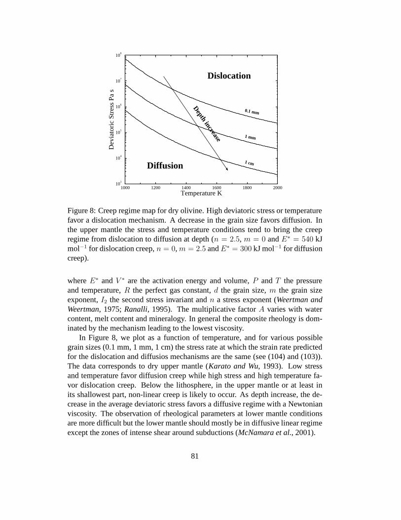
1000 1200 1400 1600 1800 2000Temperature K

103

104

105

106

107

108

Dev

iato

ric S

tres

s P

a s

Dislocation

1 cm

1 mm

0.1 mm

Diffusion

Depth increase

Figure 8: Creep regime map for dry olivine. High deviatoric stress or temperaturefavor a dislocation mechanism. A decrease in the grain size favors diffusion. Inthe upper mantle the stress and temperature conditions tendto bring the creepregime from dislocation to diffusion at depth (n = 2.5, m = 0 andE∗ = 540 kJmol−1 for dislocation creep,n = 0,m = 2.5 andE∗ = 300 kJ mol−1 for diffusioncreep).

whereE∗ andV ∗ are the activation energy and volume,P andT the pressureand temperature,R the perfect gas constant,d the grain size,m the grain sizeexponent,I2 the second stress invariant andn a stress exponent (Weertman andWeertman, 1975;Ranalli, 1995). The multiplicative factorA varies with watercontent, melt content and mineralogy. In general the composite rheology is dom-inated by the mechanism leading to the lowest viscosity.

In Figure 8, we plot as a function of temperature, and for various possiblegrain sizes (0.1 mm, 1 mm, 1 cm) the stress rate at which the strain rate predictedfor the dislocation and diffusios mechanisms are the same (see (104) and (103)).The data corresponds to dry upper mantle (Karato and Wu, 1993). Low stressand temperature favor diffusion creep while high stress andhigh temperature fa-vor dislocation creep. Below the lithosphere, in the upper mantle or at least inits shallowest part, non-linear creep is likely to occur. Asdepth increase, the de-crease in the average deviatoric stress favors a diffusive regime with a Newtonianviscosity. The observation of rheological parameters at lower mantle conditionsare more difficult but the lower mantle should mostly be in diffusive linear regimeexcept the zones of intense shear around subductions (McNamara et al., 2001).

81

The lateral variations of viscosity due to each separate parameter, stress ex-ponent, temperature, water content or grain size can potentially be very large.Surprisingly, attempts to deduce these variations directly from geodynamic obser-vations have not be very successful. Attempts to explain theEarth’s gravity frominternal loads do not seem to require lateral viscosity variations in the deep mantle(Zhang and Christensen, 1993). Near the surface, viscosity variations are present,at least between continental and oceanic lithosphere (Ricard et al., 1991;Cadekand Fleitout, 2003). The gain in fitting the Earth’s gravity or post glacial rebounddata with 3D viscosity models remains rather moderate compared to the complex-ities added to the modeling (Gasperini et al., 2004) and most models of mantleviscosity are restricted to radial profiles (Mitrovica and Forte, 1997). Even themodeling of slabs, their curvatures and their stress patterns do not really requirethat they are much stiffer than the surrounding mantle (Tao and Oconnell, 1993).

6.3.1 Temperature dependence of viscosity

The viscosity is a strong function of temperature and the cold lithosphere seems tohave a viscosity of order 1025 Pa s (Beaumont, 1978), 4 to 6 orders of magnitudestiffer than the asthenosphere. The activation energyE∗ is typically from 300 to600 kJ mol−1 (Drury and FitzGerald, 1998) the lowest values being for diffusioncreep. This implies a factor∼10 in viscosity decrease for a 100 K temperatureincrease (usingT ∼ 1600 K). The effect of temperature dependence of viscosityon the planform of convection was recognized experimentally using oils or syrups(Booker, 1976;Richter, 1978;Nataf and Richter, 1982). In the case of a stronglytemperature dependent viscosity, the definition of the Rayleigh number is ratherarbitrary as the maximum, the minimum or some average viscosity can be cho-sen in its definition. Another nondimensional number (e.g.,the ratio of viscosityvariations,µmax/µmin) must be known to characterize the convection.

Not surprisingly, two extreme regimes are found. For a viscosity ratio lowerthan about 100, the convection pattern remains quite similar to convection withuniform viscosity. On the other hand, if the viscosity of thecold boundary layer(the lithosphere) is more than 3000 times that of the underlying asthenosphere,the surface becomes stagnant (Solomatov, 1995). Below this immobile lid, theflow resembles convection below a rigid top surface (Davaille and Jaupart, 1993).In between, when the viscosity ratios are in the range 100-3000, the lithospheredeforms slowly and in this sluggish regime, the convection cells have large aspectratios.

Convection with temperature-dependent viscosity has beeninvestigated byvarious authors (Parmentier et al., 1976;Christensen, 1984b;Tackley et al., 1993;Trompert and Hansen, 1998b;Kameyama and Ogawa, 2000). Since the topboundary layer is stiffer than the bottom boundary layer, the top boundary layer

82

is also thicker than the bottom one. This impedes surface heat removal, eases theheat flux across the bottom boundary layer, and raises the average mantle temper-ature. Convection patterns computed withT -dependent viscosity remain howeverquite far from Earth-like convection. The major differenceis that when theT -dependence is too strong, the surface freezes and becomes immobile while on thereal Earth, the lithosphere is highly viscous but broken into tectonic plates sepa-rated by weak boundaries. Without mechanisms other than a simpleT -dependenceof viscosity, the Earth would be in a stagnant-lid regime.

Various modelers have thus tried to useT -dependent rheologies but have im-posed a plate-like surface velocity. This has been very useful to understand theinitiation of subduction (Toth and Gurnis, 1998), the interaction of slabs with thephase changes in the transition zone (Christensen, 1996, 1997b) and the relation-ship between subduction and gravity (King and Hager, 1994). These numericalexperiments, mostly intended to model slabs, compare satisfactorily with labora-tory experiments (Kincaid and Olson, 1987;Guilloufrottier et al., 1995).

To conclude this brief section on temperature dependence ofviscosity we dis-cuss the general concept of self-regulation of planetary interiorsTozer(1972). Ifa planet were convecting too vigorously it would lose more heat than radioac-tively produced. It would therefore cool down until the viscosity is large enoughto reduce the heat transfer. On the contrary, a too slowly convecting planet wouldnot extract its radioactive energy, and would heat up until the viscosity is reducedsufficiently (see also Chapter 2). The internal temperatureof planets is mostlycontroled to the activation energy (or rather enthalpy) of the viscosity (assumingthat planets have similar amount of heat sources). To first order, large and smallterrestrial rocky planets probably have the same internal temperatures.

6.3.2 Depth-dependence of viscosity

The activation volume of the viscosity is typically around 10−5 m3 mol−1. Ex-trapolating to CMB conditions, this suggests a large viscosity increase throughoutthe mantle. However measurements of viscosity at both highT andP conditionsare very difficult. The viscosity increase by a factor 30 to 100 suggested by geo-dynamics (see paragraph 6.1 and Chapter 7) is probably a constrain as robust aswhat could be deduced from mineralogic experiments.

The effect of a depth dependent viscosity on the planform of convection hasbeen studied by e.g.,Gurnis and Davies(1986);Cserepes(1993) orDubuffet et al.(2000). At least two important geodynamic observations canbe explained by anincrease of viscosity with depth. One is the relative stability of hotspots. A slug-gish lower mantle where convection is decreased in intensity by a larger viscosity(and also by a smaller expansivity and a potentially larger thermal conductivityas discussed in section 6.5.3) favors the relative hotspot fixity (Richards, 1991;

83

Steinberger and O’Connell, 1998). A second consequence is a depth dependenceof the wavelengths of the thermal heterogeneities. A viscosity increase (togetherwith the existence of plates and continents that impose their own wavelengths, see6.7), induces the existence of large-scale thermal anomalies at depth (Bunge andRichards, 1996). A slab crossing a factor 30-100 viscosity increase should thickenby a factor of order 3-5Gurnis and Hager(1988). This thickening is observed intomographic models (van der Hilst et al., 1997) and can be inferred from geoidmodeling (Ricard et al., 1993a).

6.3.3 Stress-dependence of viscosity

Starting fromParmentier et al.(1976) the effect of a stress-dependent viscosityhas been studied byChristensen(1984a);Malevsky and Yuen(1992);van Kekenet al.(1992);Larsen et al.(1993), assuming either entirely non-linear or compos-ite rheologies (where deformation is accommodated by both linear and non-linearmechanisms). At moderate Rayleigh number, the effect of a non-linear rheologyis not very significant. In fact, the non-linearity in the rheology is somewhat op-posed to the temperature-dependence of the rheology. As shown by Christensen(1984a), aT -dependent, non-linear rheology with an exponentn ∼ 3 leads toconvection cells rather similar to what would be obtained with a linear rheologyand an activation energy divided by∼ n. Convection with both non-linear andT -dependent rheology looks more isoviscous than convectionwith only stress-dependent or onlyT -dependent, rheologies.

At large Rayleigh number, however, non-linear convection becomes more un-stable (Malevsky and Yuen, 1992) and the combination of non-linear rheology,T -dependent rheology and viscous dissipation can accelerate the rising velocityof hot plumes by more than an order of magnitude (Larsen and Yuen, 1997).

6.3.4 Grain size dependence of viscosity

The factorA of the viscosity law (245), can also be strongly variable andit is forexample a function of the grain sized with A ∝ dm andm of order3 in the diffu-sion regime (Karato et al., 1986) (when the rheology is linear in terms of stress, itbecomes non-linear in terms of grain size). There is a clear potential feed back in-teraction between deformation, grain size reduction by dynamic recrystallization,viscosity reduction and further localization (Jaroslow et al., 1996). Grain size re-duction is balanced by Ostwald ripening (e.g., the fact thatsurface energy drivesdiffusion from small grains to larger grains) which provides a healing mechanismto increase on the long term the average size of grains (Hillert , 1965). This in-crease of the average size of grains is in fact obtained by thedecrease in size ofsmall grains by dissolution into larger ones.

84

A grain size-dependent viscosity has been introduced into geodynamic models(e.g.,Braun et al., 1999;Kameyama et al., 1997). The effect is potentially impor-tant in the mantle and even more important in the lithosphere. However, up tonow, the basic physics remains problematic since the general conservation equa-tions and the empirical laws of grain size evolution are not self consistent. Thechanges in surface energy cannot be easily accounted for in the total energy con-servation and the experimental laws of grain reduction (in the dislocation regime)and viscosity reduction and healing (in the diffusion regime) have been obtainedin mutually exclusive conditions.

6.4 Importance of sphericity

An obvious difference between the convection planform in a planet and in an ex-perimental tank is due to the sphericity of the former. In thecase of purely heatedfrom below convection, the same heat flux (in a statistical sense) has to be trans-ported through the bottom boundary layer and the top boundary layer. Howeveras the CMB surface is about 4 times smaller than the top surface, this implies a 4times larger thermal gradient through the bottom boundary layer than across thelithosphere. A bottom boundary layer thicker than the top boundary layer rein-forces the upwelling hot instabilities with respect to the downgoing cold instabil-ities. Sphericity affects the average temperature and the top and bottom boundarylayer thicknesses in a way totally opposite to the effects ofinternal sources (see6.2) orT -dependent viscosity (see 6.3). Although numerically moredifficult tohandle, spherical convection models are more and more common (Bercovici et al.,1989b;Tackley et al., 1993;Bunge et al., 1997;Zhong et al., 2000). Figure 9 is anexample of the complex patterns that can be obtained with convection in a sphere.

6.5 Other depth-dependent parameters

6.5.1 Thermal expansivity variations

The thermal expansivity varies with depth, as predicted by the EoS (80), fromwhich we can easily deduce that

α =α0

(ρ/ρ0)n−1+q + α0(T − T0). (246)

It decreases with both temperature and density, and thus with depth. The expan-sivity varies from∼ 4 × 10−5 K−1 near the surface to∼ 8 × 10−6 K−1 nearthe CMB (Chopelas and Boehler, 1992). This diminishes the buoyancy forces

85

Figure 9: Isothermal surfaces in a spherical convection model (simulations byMarc Monnereau, cold=blue, yellow and orange=hot). Cold sheet like down-wellings are sinking from the surface. Large-scale upwellings are reaching theupper-lower mantle interface. The presence of a phase change (see below 6.6),impedes the large hotspot penetration but generates secondary smaller plumes inthe upper mantle.

86

and slows down the deep mantle convection (Hansen et al., 1993). Like the in-crease of viscosity with depth, a depth-dependent thermal expansivity broadensthe thermal structures of the lower mantle, and suppresses some hot instabilitiesat the CMB. On the other hand, hot instabilities gain buoyancy as they rises in themantle which favors their relative lateral stationarity. In addition to its averagedepth dependence, the temperature dependence of the expansivity also affects thebuoyancy of slabs (Schmeling et al., 2003).

6.5.2 Increase in average density with depth

To take into account the depth dependence of density, the Boussinesq approxi-mation has be replaced by the anelastic approximation. The investigations havebeen carried out byBercovici et al.(1992) and since extended to higher Rayleighnumbers (e.g.,Balachandar et al., 1992, 1993;Zhang and Yuen, 1996).

One of the difficulties with compressible fluids is that the local criterion forinstability, (see 4.3.3), is related to the adiabatic gradient. Depending on assump-tions about the curvature of the reference geotherm with depth (the slope of theadiabatic gradient), part of the fluid can be unstable while the other part is stable.Assuming a uniform adiabatic gradient does not favor the preferential destabiliza-tion of either the upper or the lower mantle. On the other hand, assuming that thereference temperature increases exponentially with depth(i.e., taking the order ofmagnitude equations (120) as real equalities) would lead toan easier destabiliza-tion of the top of the mantle than of its bottom as a much largerheat flux would becarried along the lower mantle adiabat. In the real Earth, the adiabatic gradient, (inK km−1), should decrease with depth (due to the decrease in expansivity α withdepth insufficiently balanced by the density increase, see (118)). Since less heatcan be carried out along the deep mantle adiabat, compressibility should favor thedestabilization of the deep mantle.

Compressible convection models generally predict downgoing sheets and cylin-drical upwellings reminiscent of slabs and hotspots (Zhang and Yuen, 1996). Vis-cous dissipation is positive (as an entropy-related source) but maximum just be-low the cold boundary layer and just above the hot boundary layer, where risingor sinking instabilitities interact with the layered structures of the boundary lay-ers. On the contrary the adiabatic source heats the downwellings and cools theupwellings. On average, it reaches a maximum absolute valuein the mid-mantle.Locally, viscous dissipation and adiabatic heatings can belarger than radiogenicheat production although integrated other the whole mantleand averaged overtime, the adiabatic and dissipative sources cancel out (see(57)).

87

6.5.3 Thermal conductivity variations

The thermal conductivity of a solid is due to two different effects. First, a hotmaterial produces blackbody radiation that can be absorbedby neighboring atoms.This radiative transport of heat is probably a minor component since the meanfree path of photons in mantle materials is very small. Second, phonons, whichare collective vibrations of atoms, are excited and can dissipate their energiesby interacting with other phonons, with defects and with grain boundaries. Thefree paths of phonons being larger, they are the main contributors to the thermalconductivity.

According toHofmeister(1999), thermal conductivity should increase withdepth by a factor∼2-3. The recent observations of phase transitions in the bottomof the lower mantle should also be associated with another conductivity increase(Badro et al., 2004). This is one more effect (with the viscosity increaseandthe thermal expansivity decrease) that should decrease thedeep mantle convec-tive vigor. It also broadens the thermal anomalies, increases the average mantletemperature and thins the bottom boundary layer (Dubuffet et al., 1999).

6.6 Thermo-chemical convection

Except in section 5, a simple negative relationship was assumed between den-sity variations and temperature variations, through the thermal expansivity,∆ρ =−α∆T . However, in the mantle several sources of density anomalies are present.The density in the mantle varies with the temperatureT for a given mineralogi-cal composition, or phase content, symbolized by the symbolφ (e.g., for a givenproportion of oxides and perovskite in the lower mantle). The mineralogy for agiven bulk elemental compositionχ (e.g., the proportion of Mg, Fe, O... atoms),evolves with pressure and temperature to maintain the Gibbsenergy minimum.The variations of density in the mantle at a given pressure, have potentially threecontributions that can be summarized as

∆ρ =

(

∂ρ

∂T

)

φ

∆T +

(

∂ρ

∂φ

)

T

(

∂φ

∂T

)

χ

∆T +

(

∂ρ

∂φ

)

T

(

∂φ

∂χ

)

T

∆χ (247)

The first term on the right side is the intrinsic thermal effect computed assuminga fixed mineralogy. We have already discussed this term. The second term is athermochemical effect. The density is a function of the mineralogical composi-tion contoled at uniform pressure and elemental composition, by the temperaturevariations. This term is responsible for a rise of the 410 km depth interface anddeepens the 660 km depth interface in the presence of cold downwellings (Irifuneand Ringwood, 1987). The last term is the intrinsic chemical effect (related to

88

variations of the mineralogy due to changes in the elementalcomposition at con-stant temperature). The three contributions have very similar amplitudes and noneof them is negligible (Ricard et al., 2005).

The effect of the second term has been rather well studied (Schubert et al.,1975;Christensen and Yuen, 1984;Machetel and Weber, 1991;Peltier and Sol-heim, 1992;Tackley et al., 1993;Tackley, 1995;Christensen, 1996). Phase changesin cold downgoing slabs occur at shallower depth in the case of exothermic phasechanges and at greater depth for endothermic phase changes (the ringwoodite tooxides plus perovskite phase change at 660 km depth is endothermic, all the im-portant other phase changes of the transition zone are exothermic). These sourcesof anomalies and their signs are related to the Clapeyron slope of the phase tran-sitions. The existence of latent heat release during phase change (see (158)) is asecondary and minor effect. The recent discovery of a phase transformation in thedeep lower mantle (Murakami et al., 2004) (the post-perovskite phases) suggeststhat part of the complexities of the D” layer are related to the interaction betweena phase change and the hot boundary layer of the mantle (Nakagawa and Tackley,2006).

The fact that below the normal 660 km depth interface there isa region whereslabs remain in a low density upper-mantle phase instead of being transformedinto the dense lower mantle phase is potentially a strong impediment to slab pen-etration. The idea that this effect induces a layering of convection at 660 kmdepth or a situation where layered convection is punctuatedby large ”avalanche”events dates back toRingwood and Irifune(1988) and was supported by numericalsimulations in the nineties. It seems however that the importance of this poten-tial effect has been reduced in recent simulations with morerealistic Clapeyronslopes, phase diagrams (taking into account both the pyroxene and garnet phases),thermodynamic reference values (the phase change effect has to be compared withthermal effects and thus an accurate choice for the thermal expansivity is neces-sary), and viscosity profiles.

The last contribution to the density anomalies are related to variations in chem-ical composition. There are indications of large-scale depth and lateral variationsof Fe or Si contents in the mantle (Bolton and Masters, 2001;Saltzer et al., 2004).A large well-documented elemental differentiation is between the oceanic crust(poor in Mg, rich in Al and Si) and the mantle. The density differences between anormal pyrolitic mantle and an oceanic basalt, both at lowermantle pressure (andappropriate mineralogical phases) is larger than the thermal density variations thatcan be expected in the mantle. The oceanic crust in its high pressure eclogitic fa-cies, is∼ 5% denser that the average mantle density in most of the mantle exceptin the shallowest 100 kilometers of the lower mantle where itis lighter (Irifuneand Ringwood, 1993). In the deepest mantle it is not yet totally clear whether theeclogite remains denser, neutrally buoyant or even slightly lighter than the average

89

mantle (e.g.,Ricolleau et al., 2004). Since the thermal expansivity decreases withdepth the compositional density variations, though small,remain important in thelower mantle. Thermochemical simulations starting with the pioneering paper ofChristensen and Hofmann(1994) show the possibility of a partial segregation ofoceanic crust during subduction, forming pyramidal piles on the CMB. These re-sults have been confirmed by e.g.,Tackley(2000) andDavies(2002). These com-positional pyramids may anchor the hotspots (Jellinek and Manga, 2002;Davailleet al., 2002). The presence of a petrologically dense component ofthe sourceof hotspots also seems necessary to explain their excess temperature (Farnetani,1997).

Not only present-day subductions can generate compositional anomalies in themantle. Geochemists have often argued for a deep layer of primitive material. Thislayer should be intrinsically denser to resist entrainmentby convection. The sta-bility of such a layer has been discussed by various authors (Davaille, 1999;Kel-logg et al., 1999;Tackley and Xie, 2002;LeBars and Davaille, 2002;Samuel andFarnetani, 2003). Depending of the ratio between the intrinsic density increaseto the thermal density variations, a deep layer may be stable, slowly eroded, mayundergo large oscillating motions (the so-called lava-lamp mode of thermochem-ical convection), or be rapidly mixed. Numerical simulations of thermo-chemicalconvection are certainly going to replace the thermal convection models in thenext years. They will help to bridge the gap between geochemical observationsand convection modeling (Coltice and Ricard, 1999;van Keken et al., 2002).

6.7 A complex lithosphere: plates and continents

The lithosphere is part of the convection cell and plate tectonics and mantle con-vection cannot be separated. The role and specifics of the lithosphere are complexand are more deeply discussed in Chapter 8.

The fact that the cold lithosphere is much more viscous and concentrates mostof the mass heterogeneities of the mantle, makes it behavingby some aspect asa membrane on top of a less viscous fluid. This suggests some analogy betweenmantle convection and what is called Marangoni convection (Marangoni, 1840-1925). Marangoni convection (Nield, 1964) is controlled by temperature depen-dent surface tension on top of thin layers of fluids.

The Earth’s mantle is certainly not controlled by surface tension. Marangoniconvection, strictly speaking has nothing to do with mantleconvection. Howeverthe equations of thermal convection with cooling from the top and with a highlyviscous lithosphere can be shown to be mathematically close(through a change ofvariables) to those of Marangoni convection (Lemery et al., 2000). This analogyhas been advocated as a ”top-down” view of the mantle dynamics (Anderson,2001). More classically, the interpretation of plate cooling in terms of ridge-push

90

force (Turcotte and Schubert, 1982), or the analysis of tectonic stresses using thinsheet approximations (England and Mckenzie, 1982) belong to the same approach.

Due to the complexities of the lithosphere properties, the boundary conditionat the surface of the Earth is far from being a uniform free-slip condition. Bothcontinents and tectonic plates impose their own wavelengths and specific bound-ary conditions on the underlying convecting asthenosphere. Of course the positionof the continents and the number and shape of the plates are themselves, conse-quences of mantle convection. The plates obviously organize the large scale flowin the mantle (Hager and Oconnell, 1979;Ricard and Vigny, 1989). They imposea complex boundary condition where the angular velocity is piece-wise constant.The continents with their reduced heat flow (Jaupart and Mareschal, 1999) alsoimpose a laterally variable heat flux boundary condition.

Convection models with continents have been studied numerically (Gurnisand Hager, 1988;Grigne and Labrosse, 2001) and experimentally (Guillou andJaupart, 1995). Continents with their thick lithosphere tend to increase the thick-ness of the top boundary layer and the temperature below them(see Figure 10).Hot rising currents are predicted under continents and downwellings are localizedalong continental edges. The existence of a thick and stablecontinental root mustbe due to a chemically lighter and more viscous subcontinental lithosphere (Doinet al., 1997). The ratio of the heat flux extracted across continents compared tothat extracted across oceans increases with the Rayleigh number. This suggeststhat the continental geotherms were not much different in the past when the ra-diogenic sources were larger; it is mostly the oceanic heat flux that was larger(Lenardic, 1998). Simulating organized plates self-consistently coupled with aconvective mantle has been a very difficult quest. The attempts to generate platesusingT -dependent or simple non-linear rheologies have failed. Although in 2Dsome successes can be obtained in localizing deformation inplate-like domains,(Schmeling and Jacoby, 1981;Weinstein and Olson, 1992;Weinstein, 1996), theyare obtained with stress exponents (e.g.,n ≥ 7) that are larger than what can beexpected from laboratory experiments (n ∼ 2). The problems are however worstin 3D. Generally these early models do not predict the important shear motionsbetween plates that we observe (Christensen and Harder, 1991;Ogawa et al.,1991).

Some authors have tried to mimic the presence of plates by imposing plate-like surface boundary conditions. These studies have been performed in 2D and3D (Ricard and Vigny, 1989;Gable et al., 1991;King et al., 1992;Monnereau andQuere, 2001). Although they have confirmed the profound effect of plates on thewavelengths of convection, on its time-dependence and on the surface heat flux,these approaches cannot predict the evolution of surface plate geometry. Figure11 illustrates the organizing effect of plates in spherical, internally heated com-pressible convection with depth dependent viscosity (Bunge and Richards, 1996).

91

Figure 10: Convection patterns in the presence of 4 continents. The total aspectratio is 7, the continents are defined by a viscosity increaseby a factor 103 overthe depth 1/10. The viscosity is otherwise constant. The Rayleigh number basedon the total temperature drop (bottom panels) or on the internal radioactivity (toppanels) is 107. The downwellings are localized near the continent margins. Alarge difference in heat flux is predicted between oceans andcontinents. In thecase of bottom heating, hotspots tend to be preferentially anchored below conti-nents where they bring an excess heat. This tends to reduce the surface heat fluxvariations.

92

To obtain a self-consistent generation of surface plates, more complex rheologiesthat include brittle failure, strain-softening and damagemechanisms must be in-troduced (e.g.,Moresi and Solomatov, 1998;Auth et al., 2003). The existenceof plates seems also to require the existence of a weak sub-lithospheric astheno-sphere (Richards et al., 2001). In the last years, the first successes in computing3D models that spontaneously organize their top boundary layer into plates havebeen reached (Tackley, 1998;Trompert and Hansen, 1998a;Stein et al., 2004). Al-though the topological characteristics of the predicted plates and their time evolu-tion may be still far from the observed characteristics of plate tectonics, and oftentoo episodic (stagnant-lid convection punctuated by plate-like events), a very im-portant breakthrough has been made by modelers (see Figure 12).

The Earth’s plate boundaries keep the memory of their weakness over geologi-cal times (Gurnis et al., 2000). This implies that the rheological properties cannotbe a simple time-independent function of stress or temperature but has a long termmemory. The rheologies that have been used to predict platesin convective mod-els remain empirical and their interpretation in terms of microscopic behavior anddamage theory remains largely to be done (Bercovici and Ricard, 2005).

Acknowledgements:This chapter benefited from a very careful check of the equations by FredericChambat, and from detailed and constructive reviews by NeilRibe and GerrySchubert. I also thank Ondrej Sramek, William Landhuy, Nicolas Coltice, FabienDubuffet, David Bercovici and probably others for their comments and sugges-tions.

References

Anderson, D. L. (2001), Geophysics - Top-down tectonics?,Science, 293, 2016–2018.

Anderson, O. L. (1979), Evidence supporting the approximation γρ = const for thegruneisen parameter of the earth lower mantle,J. Geophys. Res., 84, 3537–3542.

Auth, C., D. Bercovici, and U. R. Christensen (2003), Two-dimensional convection witha self-lubricating, simple-damage rheology,Geophys. J. Int., 154, 783–800.

93

Figure 11: This figure depicts spherical compressible internally heated convectionmodels where the viscosity increases with depth (simulations by Peter Bunge). Inthe first row, a uniform free-slip condition on top has been used. In the second row,the present day observed plate motion is imposed at the surface. The left columnshows the temperature field in the middle of the upper mantle,the right column inthe middle of the lower mantle. This figure summarizes various points discussedin the text: the presence of linear cold downwellings, the absence of active up-wellings in the absence of basal heating, the enlargement ofthermal structure inthe more viscous lower mantle (top row). Although the modeling is not self con-sistent (i.e., the presence of plates and the constancy of plate velocities are totallyarbitrary) it is clear that the presence of plates can changeradically the convectionpatterns (compare top and bottom rows).

94

Figure 12: Convection models with self-coherent plate generation (Stein et al.,2004). Snapshot of the temperature field for a model calculation in a box of aspectratio 4. The viscosity is temperature, pressure and stress dependent. The flowpattern reveals cylindrical upwellings and sheet-like downflow. Three plates haveformed sketched in the small plot.

95

Badro, J., J. P. Rueff, G. Vanko, G. Monaco, G. Fiquet, and F. Guyot (2004), Electronictransitions in perovskite: Possible nonconvecting layersin the lower mantle,Science,305, 383–386.

Bai, W. M., C. Vigny, Y. Ricard, and C. Froidevaux (1992), On the origin of deviatoricstresses in the lithosphere,J. Geophys. Res., 97, 11,729–11,737.

Balachandar, S., D. A. Yuen, and D. Reuteler (1992), Time-dependent 3-dimensionalcompressible convection with depth-dependent properties, Geophys. Res. Lett., 19,2247–2250.

Balachandar, S., D. A. Yuen, and D. Reuteler (1993), Viscousand adiabatic heating effectsin 3-dimensional compressible convection at infinite prandtl number,Phys. Fluids A-fluid Dynamics, 5, 2938–2945.

Barenblatt, G. I. (1996),Scaling, Cambridge University Press.

Batchelor (1967),An Introduction to Fluid Dynamics, Cambridge University Press.

Beaumont, C. (1978), Evolution of sedimentary basins on a viscoelastic lithosphere -theory and examples,Geophys. J. Royal Astron. Soc., 55, 471–497.

Becker, T. W., and L. Boschi (2002), A comparison of tomographic and geodynamicmantle models,Geochem. Geophys. Geosyst., 3, 2001GC000,168.

Bercovici, D., and S. Karato (2003), Whole-mantle convection and the transition-zonewater filter,Nature, 425, 39–44.

Bercovici, D., and Y. Ricard (2003), Energetics of a two-phase model of lithosphericdamage, shear localization and plate-boundary formation,Geophys. J. Int., 152, 581–596.

Bercovici, D., and Y. Ricard (2005), Tectonic plate generation and two-phase damage:Void growth versus grain size reduction,J. Geophys. Res., 110.

Bercovici, D., G. Schubert, and G. A. Glatzmaier (1989a), Three dimensional sphericalmodels of convection in the earth’s mantle,Science, 244, 950–955.

Bercovici, D., G. Schubert, and G. A. Glatzmaier (1989b), 3-dimensional spherical-models of convection in the earths mantle,Science, 244, 950–955.

Bercovici, D., G. Schubert, and G. A. Glatzmaier (1992), 3-dimensional convection of aninfinite-prandtl-number compressible fluid in a basally heated spherical-shell,J. FluidDyn., 239, 683–719.

96

Bercovici, D., Y. Ricard, and M. Richards (2000),The relation between mantle dynamicsand plate tectonics: A primer, in: History and Dynamics of Global Plate Motions,Geophys. Monogr. Ser., vol. 121, 5–46 pp., M.A. Richards, R. Gordon, and R. van derHilst, AGU, Washington D.C.

Bercovici, D., Y. Ricard, and G. Schubert (2001a), A two-phase model of compaction anddamage, 1. general theory,J. Geophys. Res., 106, 8887–8906.

Bercovici, D., Y. Ricard, and G. Schubert (2001b), A two-phase model for compaction anddamage 3. Applications to shear localization and plate boundary formation,J. Geophys.Res., 106, 8925–8939.

Besse, J., and V. Courtillot (1991), Revised and synthetic apparent polar wander paths ofthe african, eurasian, north-america and indian plates, and true polar wander since 200ma,J. Geophys. Res., 96, 4029–4050.

Birch, F. (1952), Elasticity and constitution of the earth’s interior,J. Geophys. Res., 57,227–286.

Bolton, H., and G. Masters (2001), Travel times of P and S fromthe global digital seismicnetworks: Implications for the relative variation of P and Svelocity in the mantle,J.Geophys. Res., 106, 13,527–13,540.

Booker, J. R. (1976), Thermal-convection with strongly temperature-dependent viscosity,J. Fluid Dyn., 76, 741–754.

Braun, J., J. Chery, A. Poliakov, D. Mainprice, A. Vauchez, A. Tomassi, and M. Daig-nieres (1999), A simple parameterization of strain localization in the ductile regimedue to grain size reduction: A case study for olivine,J. Geophys. Res., 104, 25,167–25,181.

Buffett, B. A., E. J. Garnero, and R. Jeanloz (2000), Sediments at the top of Earth’s core,Science, 290, 1338–1342.

Bullen, K. E. (1940), The problem of the earth’s density variation,Seismol. Soc. Am. Bull.,30, 235–250.

Bunge, H. P., and M. A. Richards (1996), The origin of large scale structure in mantleconvection: Effects of plate motions and viscosity stratification,Geophys. Res. Lett.,23, 2987–2990.

Bunge, H. P., M. A. Richards, and J. R. Baumgardner (1997), A sensitivity study of three-dimensional spherical mantle convection at 10(8) Rayleighnumber: Effects of depth-dependent viscosity, heating mode, and an endothermic phase change,J. Geophys. Res.,102, 11,991–12,007.

97

Bunge, H. P., Y. Ricard, and J. Matas (2001), Non-adiabaticity in mantle convection,Geophys. Res. Lett., 28, 879–882.

Cadek, O., and L. Fleitout (2003), Effect of lateral viscosity variations in the top 300 kmon the geoid and dynamic topography,Geophys. J. Int., 152, 566–580.

Choblet, G., and E. M. Parmentier (2001), Mantle upwelling and melting beneath slowspreading centers: effects of variable rheology and melt productivity,Earth Planet. Sci.Lett., 184, 589–604.

Chopelas, A., and R. Boehler (1992), Thermal expansivity inthe lower mantle,Geophys.Res. Lett., 19, 1983–1986.

Christensen, U. (1984a), Convection with pressure-dependent and temperature-dependentnon-newtonian rheology,Geophys. J. Royal Astron. Soc., 77, 343–384.

Christensen, U. R. (1984b), Heat-transport by variable viscosity convection and implica-tions for the earths thermal evolution,Phys. Earth Planet. Inter., 35, 264–282.

Christensen, U. R. (1996), The influence of trench migrationon slab penetration into thelower mantle,Earth Planetary Science Lett., 140, 27–39.

Christensen, U. R. (1997a), Some geodynamical effects of anisotropic viscosity,Geophys.J. Royal Astron. Soc., 91, 711–736.

Christensen, U. R. (1997b), Influence of chemical buoyancy on the dynamics of slabs inthe transition zone,J. Geophys. Res., 102, 22,435–22,443.

Christensen, U. R., and H. Harder (1991), 3-d convection with variable viscosity,Geo-phys. J. Int., 104, 213–226.

Christensen, U. R., and A. Hofmann (1994), Segregation of subducted oceanic crust inthe convecting mantle,J. Geophys. Res., 99, 19,867–19,884.

Christensen, U. R., and D. A. Yuen (1984), The interaction ofa subducting lithosphericslab with a chemical or phase-boundary,J. Geophys. Res., 89, 4389–4402.

Colin, P., and L. Fleitout (1990), Topography of the ocean-floor - thermal evolution ofthe lithosphere and interaction of deep mantle heterogeneities with the lithosphere,Geophys. Res. Lett., 17, 1961–1964.

Coltice, N., and Y. Ricard (1999), Geochemical observations and one layer mantle con-vection,Earth Planetary Science Lett., 174, 125–137.

Connolly, J. A. D., and Y. Y. Podladchikov (1998), Compaction-driven fluid flow in vis-coelastic rock,Geodinamica Acta, 11, 55–84.

98

Corrieu, V., C. Thoraval, and Y. Ricard (1995), Mantle dynamics and geoid green-functions,Geophys. J. Int., 120, 516–523.

Cserepes, L. (1993), Effect of depth-dependent viscosity on the pattern of mantle convec-tion, Geophys. Res. Lett., 20, 2091–2094.

Davaille, A. (1999), Two-layer thermal convection in viscous fluids,J. Fluid Dyn., 379,223–253.

Davaille, A., and C. Jaupart (1993), Transient high-rayleigh-number thermal-convectionwith large viscosity variations,J. Fluid Dyn., 253, 141–166.

Davaille, A., F. Girard, and M. LeBars (2002), How to anchor hotspots in a convectingmantle?,Earth Planet. Sci. Lett., 203, 621–634.

Davies, G. F. (1980), Thermal histories of convective earthmodels and constraints onradiogenic heat-production in the earth,J. Geophys. Res., 85, 2517–2530.

Davies, G. F. (1999),Davies, G. F., 1999, Dynamic Earth Plates, Plumes and MantleConvection, Cambridge University Press, 458 p.

Davies, G. F. (2002), Stirring geochemistry in mantle convection models with stiff platesand slabs,Geochimica Et Cosmochimica Acta, 66, 3125–3142.

de Groot, S. R., and P. Mazur (1984),Non-Equilibrium Thermodynamics, Dover Publica-tions, New York.

Doin, M. P., L. Fleitout, and U. Christensen (1997), Mantle convection and stability ofdepleted and undepleted continental lithosphere,J. Geophys. Res., 102, 2771–2787.

Dombre, T., U. Frisch, J. M. Greene, M. Henon, A. Mehr, and A. M. Soward (1986),Chaotic streamlines in the abc flows,J. Fluid Dyn., 167, 353–391.

Drew, D. A., and L. A. Segel (1971), Averaged equations for 2-phase flows,Studies InAppl. Mathematics, 50, 205–220.

Drury, M. R., and J. D. FitzGerald (1998),The Earth’s mantle: composition, structure,and evolution, chap. Mantle rheology: insights from laboratory studies of deformationand phase transition, Cambridge University Press, Cambridge, England.

Dubuffet, F., D. A. Yuen, and M. Rabinowicz (1999), Effects of a realistic mantle thermalconductivity on the patterns of 3-D convection,Earth Planet. Sci. Lett., 171, 401–409.

Dubuffet, F., M. Rabinowicz, and M. Monnereau (2000), Multiple scales in mantle con-vection,Earth Planet. Sci. Lett., 178, 351–366.

Dziewonski, A. M., and D. Anderson (1981), Preliminary reference earth model,Phys.Earth Planet. Inter., 25, 297–356.

99

England, P., and D. Mckenzie (1982), A thin viscous sheet model for continental defor-mation,Geophys. J. Royal Astron. Soc., 70, 295–321.

Farnetani, C. G. (1997), Excess temperature of mantle plumes: The role of chemicalstratification across d”,Geophys. Res. Lett., 24, 1583–1586.

Ferrachat, S., and Y. Ricard (1998), Regular vs, chaotic mantle mixing,Earth Planet. Sci.Lett., 155, 75–86.

Forte, A. M., and W. R. Peltier (1987), Plate tectonics and aspherical earth structure – theimportance of poloidal-toroidal coupling,J. Geophys. Res., 92, 3645–3679.

Forte, A. M., and W. R. Peltier (1991), Viscous flow models of global geophysical ob-servables .1. forward problems,J. Geophys. Res., 96, 20,131–20,159.

Fowler, A. C. (1985), A mathematical model of magma transport in the asthenosphere,Geophys. Astrophys. Fluid Dyn, 33, 63–96.

Fowler, A. C. (1989), Generation and creep of magma in the earth, Siam J. On Appl.Mathematics, 49, 231–245.

Gable, C. W., R. J. Oconnell, and B. J. Travis (1991), Convection in 3 dimensions withsurface plates - generation of toroidal flow,J. Geophys. Res., 96, 8391–8405.

Gasperini, P., G. D. Forno, and E. Boschi (2004), Linear or non-linear rheology in theEarth’s mantle: the prevalence of power-law creep in the postglacial isostatic readjust-ment of laurentia,Geophys. J. Int., 157, 1297–1302.

Glatzmaier, G. A. (1988), Numerical simulation of mantle convection: Time-dependent,three dimensional, compressible,spherical shell,Geophys. Astrophys. Fluid Dyn., 43,223–264.

Grigne, C., and S. Labrosse (2001), Effects of continents on Earth cooling: thermal blan-keting and depletion in radioactive elements,Geophys. Res. Lett., 28, 2707–2710.

Guillou, L., and C. Jaupart (1995), On the effect of continents on mantle convection,J.Geophys. Res., 100, 24,217–24,238.

Guilloufrottier, L., J. Buttles, and P. Olson (1995), Laboratory experiments on the struc-ture of subducted lithosphere,Earth Planet. Sci. Lett., 133, 19–34.

Gurnis, M., and G. F. Davies (1986), Numerical study of high rayleigh number convectionin a medium with depth-dependent viscosity,Geophysical J. Royal Astronomical Soc.,85, 523–541.

Gurnis, M., and B. H. Hager (1988), Controls of the structureof subducted slabs,Nature,335, 317–321.

100

Gurnis, M., L. Moresi, and R. D. Mueller (2000),The History and Dynamics of GlobalPlate Motions, Richards, M. A., Gordon, R., and van der Hilst, R.editors, chap. Modelsof mantle convection incorporating plate tectonics: The Australian region since theCretaceous, pp. 211–238, American Geophysical Union, Washongton D.C.

Haase, R. (1990),Thermodynamics of irreversible processes, Dover Publications, NewYork.

Hager, B. H., and R. W. Clayton (1989),Constraints on the structure of mantle convectionusing seismic observation, flow models and the geoid, in: Mantle Convection, PlateTectonics and Global Dynamics, W.R. Peltier, Gordon and Breach Science Publishers,New York.

Hager, B. H., and R. J. Oconnell (1979), Kinematic models of large-scale flow in theearths mantle,J. Geophys. Res., 84, 1031–1048.

Hager, B. H., and R. J. O’Connell (1981), A simple global model of plate tectonics andmantle convection,J. Geophys. Res., 86, 4843–4867.

Hager, B. H., R. W. Clayton, M. A. Richards, R. P. Comer, and A.M. Dziewonski (1985),Lower mantle heterogeneity, dynamic topography and the geoid, Nature, 313, 541–546.

Hansen, U., D. A. Yuen, S. E. Kroening, and T. B. Larsen (1993), Dynamic consequencesof depth-dependent thermal expansivity and viscosity on mantle circulations and ther-mal structure,Phys. Earth Planet. Inter., 77, 205–223.

Haskell, N. A. (1937), The viscosity of the asthenosphere,Am. J. Sci.

Hewitt, J. M., D. P. McKenzie, and N. O. Weiss (1975), Dissipative heating in convectiveflows,J. Fluid Dyn., 68, 721–738.

Hier-Majumder, S., Y. Ricard, and D. Bercovici (2006), Roleof grain boundaries inmagma migration and storage,Earth Planet. Sci. Lett., 248, 735–749.

Hillert, M. (1965), On theory of normal and abnormal grain growth, Acta Metallurgica,13, 227–235.

Hirth, G., and D. L. Kolhstedt (1996), Water in the oceanic upper mantle: implications forrheology, melt extraction and the evolution of the lithosphere,Earth Planet. Sci. Lett.,144, 93–108.

Hofmeister, A. M. (1999), Mantle values of thermal conductivity and the geotherm fromphonon lifetimes,Science, 283, 1699–1706.

Irifune, T., and A. Ringwood (1993), Phase transformationsin subducted oceanic crustand buoyancy relationships at depths of 600-800 km in the mantle, Earth Planet. Sci.Lett., 117, 101–110.

101

Irifune, T., and A. E. Ringwood (1987), Phase transformations in a harzburgite compo-sition to 26GPa: implications for dynamical behaviour of the subducting slab,EarthPlanet. Sci. Lett., 86, 365–376.

Jaroslow, G. E., G. Hirth, and H. J. B. Dick (1996), Abyssal peridotite mylonites: Impli-cations for grain-size sensitive flow and strain localization in the oceanic lithosphere,Tectonophysics, 256, 17–37.

Jarvis, G. T., and D. P. Mckenzie (1980), Convection in a compressible fluid with infiniteprandtl number,J. Fluid Dyn., 96, 515–583.

Jaupart, C., and J. C. Mareschal (1999), The thermal structure and thickness of continentalroots,Lithos, 48, 93–114.

Jeanloz, R., and S. Morris (1987), Is the mantle geotherm subadiabatic,Geophys. Res.Lett., 14, 335–338.

Jellinek, A. M., and M. Manga (2002), The influence of a chemical boundary layer on thefixity, spacing and lifetime of mantle plumes,Nature, 418, 760–763.

Kameyama, M., and M. Ogawa (2000), Transitions in thermal convection with stronglytemperature-dependent viscosity in a wide box,Earth Planet. Sci. Lett., 180, 355–367.

Kameyama, M., D. A. Yuen, and H. Fujimoto (1997), The interaction of viscous heatingwith grain-size dependent rheology in the formation of localized slip zones,Geophys.Res. Lett., 24, 2523–2526.

Karato, S. I. (1998), Seismic anisotropy in the deep mantle,boundary layers and thegeometry of mantle convection,Pure Appl. Geophys., 151, 565–587.

Karato, S. I., and P. Wu (1993), Rheology of the upper mantle:A synthesis,Science, 260,771–778.

Karato, S. I., M. S. Paterson, and J. D. F. gerald (1986), Rheology of synthetic olivineaggregates - influence of grain-size and water,J. Geophys. Res., 91, 8151–8176.

Katz, R. F., M. Spiegelman, and S. M. Carbotte (2004), Ridge migration, asthenosphericflow and the origin of magmatic segmentation in the global mid-ocean ridge system,Geophys. Res. Lett., 31.

Kelemen, P. B., G. Hirth, N. Shimizu, M. Spiegelman, and H. J.B. Dick (1997), Areview of melt migration processes in the adiabatically upwelling mantle beneathoceanic spreading ridges,Philosophical Transactions Royal Soc. London Series A-mathematical Phys. Engineering Sciences, 355, 283–318.

Kellogg, L. H., and D. L. Turcotte (1987), homogeneization of the mantle by convectivemixing and diffusion,Earth Planet. Sci. Lett., 81, 371–378.

102

Kellogg, L. H., B. H. Hager, and R. D. van der Hilst (1999), Compositional stratificationin the deep mantle,Science, 283, 1881–1884.

Kennett, B. L. N. (2001),The seismic wavefield, Cambridge University Press.

Kido, M., and T. Seno (1994), Dynamic topography compared with residual depth anoma-lies in oceans and implications for age-depth curves,Geophys. Res. Lett., 21, 717–720.

Kincaid, C., and P. Olson (1987), An experimental-study of subduction and slab migra-tion, J. Geophys. Res., 92, 13,832–13,840.

King, S. D., and B. H. Hager (1994), Subducted slabs and the geoid .1. numerical experi-ments with temperature-dependent viscosity,J. Geophys. Res., 99, 19,843–19,852.

King, S. D., C. W. Gable, and S. A. Weinstein (1992), Models ofconvection-driven tec-tonic plates - a comparison of methods and results,Geophys. J. Int., 109, 481–487.

Lago, B., and M. Rabinowicz (1984), Admittance for convection in a layered sphericalshell,Geophys. J. Royal Astron. Soc..

Lambeck, K., and P. Johnston (1998),The Earth’s mantle: composition, structure, andevolution, chap. The viscosity of the mantle, pp. 461–502, Cambridge University Press,Cambridge, England.

Landau, L., and E. Lifchitz (1980),An Introduction to Fluid Dynamics, Pergamon Press,Oxford.

Landau, L., and E. Lifchitz (2000),Theory of elasticity, Butterworth- Heinemann.

Larsen, T. B., and D. A. Yuen (1997), Fast plumeheads: Temperature-dependent versusnon-Newtonian rheology,Geophys. Res. Lett., 24, 1995–1998.

Larsen, T. B., A. V. Malevsky, D. A. Yuen, and J. L. Smedsmo (1993), Temperature-dependent newtonian and non-newtonian convection - implications for lithosphericprocesses,Geophys. Res. Lett., 20, 2595–2598.

LeBars, M., and A. Davaille (2002), Stability of thermal convection in two superimposedmiscible viscous fluids,J. Fluid Dyn., 471, 339–363.

Lee, T., D. A. Papanastassiou, and G. L. Wasserburg (1976), Demonstration of26mgexcess in allende and evidence for al26, Geophys. Res. Lett., pp. 41–44.

Lemery, C., Y. Ricard, and J. Sommeria (2000), A model for theemergence of thermalplumes in Rayleigh-Benard convection at infinite Prandtl number,J. Fluid Mechanics,414, 225–250.

Lenardic, A. (1998), On the partitioning of mantle heat lossbelow oceans and continentsover time and its relationship to the Archaean paradox,Geophys. J. Int., 134, 706–720.

103

Lestunff, Y., and Y. Ricard (1995), Topography and geoid dueto lithospheric mass anoma-lies,Geophys. J. Int., 122, 982–990.

Lithgow-Bertelloni, C., and M. Gurnis (1997), Cenozoic subsidence and uplift of conti-nents from time-varying dynamic topography,Geology, 25, 735–738.

Lithgow-Bertelloni, C., and J. H. Guynn (2004), Origin of the lithospheric stress field,J.Geophys. Res., 109, doi: 10.1029/2003JB002,467.

Lithgow-Bertelloni, C., and M. A. Richards (1998), Dynamics of cenozoic and mesozoicplate motions,Reviews of Geophys., 36, 27–78.

Lithgow-Bertelloni, C., and P. G. Silver (1998), Dynamic topography, plate driving forcesand the African superswell,Nature, 395, 269–272.

Machetel, P., and P. Weber (1991), Intermittent layered convection in a model mantle withan endothermic phase change at 670 km,Nature, 350, 55–57.

Malevsky, A. V., and D. A. Yuen (1992), Strongly chaotic non-newtonian mantle convec-tion, Geophysical Astrophysical Fluid Dynamics, 65, 149–171.

Massol, H., C. Jaupart, and D. W. Pepper (2001), Ascent and decompression of viscousvesicular magma in a volcanic conduit,J. Geophys. Res., 106, 16,223–16,240.

McDonough, W. F., and S. S. Sun (1995), The composition of theearth,Chem. Geology,120, 223–253.

McKenzie, D. (1984), The generation and compaction of partially molten rock,J. Petrol.

McNamara, A. K., S. I. Karato, and P. E. van Keken (2001), Localisation of dislocationcreep in the lower mantle: Implications for the origin of seismic anisotropy,EarthPlanet. Sci. Lett., 191, 85–99.

Mitrovica, J. X., and A. M. Forte (1997), Radial profile of mantle viscosity: Results fromthe joint inversion of convection and postglacial rebound observables,J. Geophys. Res.,102, 2751–2769.

Monnereau, M., and S. Quere (2001), Spherical shell models of mantle convection withtectonic plates,Earth Planet. Sci. Lett., 184, 575 – 588).

Moresi, L., and V. Solomatov (1998), Mantle convection witha brittle lithosphere:thoughts on the global tectonic styles of the Earth and venus, Geophys. J. Int., 133,669–682.

Muhlhaus, H. B., L. Moresi, and M. Cada (2004), Emergent anisotropy and flow align-ment in viscous rocks,Pure Appl. Geoph., 161, 2451–2463.

104

Munk, W. H., and G. J. F. MacDonald (1960),The rotation of the Earth: A geophysicaldiscussion, Cambridge.

Murakami, T., K. Hirose, K. Kawamura, N. Sata, and Y. Ohishi (2004), Post-perovskitephase transition inMgSiO3, Science, 304, 855–858.

Murnaghan, F. D. (1951),Finite deformation of an elastic solid, John Wiley and Sons,New York.

Nakagawa, T., and P. J. Tackley (2006), Three-dimensional structures and dynamics inthe deep mantle: Effects of post-perovskite phase change and deep mantle layering,Geophys. Res. Lett., 33(L12S11, doi:1029/2006GL025719).

Nataf, H. C., and F. M. Richter (1982), Convection experiments in fluids with highlytemperature-dependent viscosity and the thermal evolution of the planets,Phys. EarthPlanet. Inter., 29, 320–329.

Nield, D. A. (1964), Surface tension and buoyancy effects incellular convection,J. FluidDyn., 19, 341–352.

Nye, J. F. (1953), The flow law of ice from measurements in glacier tunnels, laboratoryexperiments and the jungfraufirn borehole experiment,Proc. Royal Soc. London SeriesA-mathematical Phys. Sciences, 219, 477–489.

Ogawa, M., G. Schubert, and A. Zebib (1991), Numerical simulations of 3-dimensionalthermal-convection in a fluid with strongly temperature-dependent viscosity,J. FluidDyn., 233, 299–328.

Olson, P., D. A. Yuen, and D. Balsiger (1984), Mixing of passive heterogeneties by mantleconvection,J. Geophys. Res., 89, 425–436.

Ottino, J. M. (1989),The kinematics of mixing: stretching, chaos and transport, Cam-bridge University Press, New-York.

Panasyuk, S., B. Hager, and A. Forte (1996), Understanding the effects of mantle com-pressibility on geoid kernels,Geophys. J. Int., 124, 121–133.

Parmentier, E. M., D. L. Turcotte, and K. E. Torrance (1976),Studies of finite-amplitudenon-newtonian thermal convection with application to convection in earths mantle,J.Geophys. Res., 81, 1839–1846.

Parmentier, E. M., C. Sotin, and B. J. Travis (1994), Turbulent 3-d thermal-convectionin an infinite prandtl number, volumetrically heated fluid - implications for mantle dy-namics,Geophys. J. Int., 116, 241–251.

Parsons, B., and S. Daly (1983), The relationship between surface topography, gravityanomaly and the temperature structure of convection,J. Geophys. Res., 88, 1129–1144.

105

Peltier, W. R. (1989),Mantle convection: plate tectonics and Global geodynamics, chap.Mantle viscosity, pp. 389–478, Gordon and Breach Science Publishers, New York.

Peltier, W. R. (1996), Mantle viscosity and ice-age ice sheet topography,Science, 273,1359–1364.

Peltier, W. R., and L. P. Solheim (1992), Mantle phase transition and layered chaoticconvection,Geophys. Res. Lett., 19, 321–324.

Poirier, J. P. (1991),Introduction to the physics of the Earth’s interior, Cambridge Uni-versity Press.

Poirier, J. P., and A. Tarantola (1998), A logarithmic equation of state,Phys. Earth Planet.Inter., 109, 1–8.

Rabinowicz, M., Y. Ricard, and M. Gregoire (2002), Compaction in a mantle with a verysmall melt concentration: Implications for the generationof carbonatitic and carbonate-bearing high alkaline mafic melt impregnations,Earth Planet. Sci. Lett., 203, 205–220.

Ranalli, G. (1995),Rheology of the Earth, Kluwer academic publishers.

Ribe, N. M. (1985a), The deformation and compaction of partial molten zones,Geophys.J. Royal Astron. Soc., 83, 487–501.

Ribe, N. M. (1985b), The generation and composition of partial melts in the earths mantle,Earth Planet. Sci. Lett., 73, 361–376.

Ricard, Y., and D. Bercovici (2003), Two-phase damage theory and crustal rock failure:the theoretical ’void’ limit, and the prediction of experimental data,Geophys. J. Int.,155, 1057–1064.

Ricard, Y., and N. Coltice (2004),Geophysical and geochemical models of mantle convec-tion: Successes and future challenges, The state of the planet: Frontiers and challengesin geophysics, vol. 150, 59-68 pp., Geophys. Monogr. Ser.

Ricard, Y., and C. Vigny (1989), Mantle dynamics with induced plate-tectonics,J. Geo-phys. Res., 94, 17,543–17,559.

Ricard, Y., L. Fleitout, and C. Froidevaux (1984), Geoid heights and lithospheric stressesfor a dynamic Earth,Ann. Geophysica, 2, 267–286.

Ricard, Y., C. Vigny, and C. Froidevaux (1989), Mantle heterogeneities, geoid and platemotion: a monte carlo inversion,J. Geophys. Res., 94, 13,739–13,754.

Ricard, Y., C. Doglioni, and R. Sabadini (1991), Differential rotation between lithosphereand mantle - a consequence of lateral mantle viscosity variations,J. Geophys. Res., 96,8407–8415.

106

Ricard, Y., M. Richards, C. Lithgow-Bertelloni, and Y. L. Stunff (1993a), A geodynamicmodel of mantle density heterogeneity,J. Geophys. Res., 98, 21,895–21,909.

Ricard, Y., G. Spada, and R. Sabadini (1993b), Polar wander of a dynamic earth,Geophys.J. Int., 113, 284–298.

Ricard, Y., D. Bercovici, and G. Schubert (2001), A two-phase model for compaction anddamage 2. Applications to compaction, deformation, and therole of interfacial surfacetension,J. Geophys. Res., 106, 8907–8924.

Ricard, Y., E. Mattern, and J. Matas (2005),Earth’s Deep Mantle: Structure, Composi-tion, and Evolution, chap. Synthetic tomographic images of slabs from mineral physics,pp. 285–302, AGU monograph, van der Hilst, Bass, Matas and Trampert eds.

Richards, M. (1991),Hotspots and the case for a high viscosity lower mantle, in GlacialIsostasy, Sea-Level and Mantle Rheology, R. Sabadini et al., eds, 571-587 pp., KluwerAcademic Publishers, Dordrecht.

Richards, M. A., and D. C. Engebretson (1992), Large-scale mantle convection and thehistory of subduction,Nature, 355, 437–440.

Richards, M. A., and B. H. Hager (1984), Geoid anomalies in a dynamic earth,J. Geophys.Res., 89, 5987–6002.

Richards, M. A., R. Y, C. Lithgow-Bertelloni, G. Spada, and R. Sabadini (1997), Anexplanation for earth’s long-term rotational stability,Science, 275, 372–375.

Richards, M. A., W. S. Yang, J. R. Baumgardner, and H. P. Bunge(2001), Role of a low-viscosity zone in stabilizing plate tectonics: Implications for comparative terrestrialplanetology,Geochem. Geophys. Geosys., 2.

Richter, F. M. (1978), Experiments on the stability of convection rolls in fluids whoseviscosity depends on temperature,J. Fluid Dyn., 89, 553–.

Richter, F. M., and D. Mckenzie (1984), Dynamical models formelt segregation from adeformable matrix,J. Geology, 92, 729–740.

Ricolleau, A., G. Fiquet, J. Perillat, I. Daniel, N. Menguy,H. Cardon, A. Addad, C. Vanni,and N. Guignot (2004), The fate of subducted basaltic crust in the earth’s lower mantle:an experimental petrological study, inEos Trans. AGU, Fall Meet. Suppl, vol. 85(47),abstract U33B-02.

Riley, G. N., D. L. Kohlstedt, and F. M. Richter (1990), Melt migration in a silicateliquid-olivine system - an experimental test of compactiontheory,Geophys. Res. Lett.,17, 2101–2104.

107

Ringwood, A. E., and T. Irifune (1988), Nature of the 650-km seismic discontinuity -implications for mantle dynamics and differentiation,Nature, 331, 131–136.

Rudnick, R. L., and D. M. Fountain (1995), Nature and composition of the continental-crust - a lower crustal perspective,Rev. Geophys., 33, 267–309.

Runcorn, S. K. (1964), Satellite gravity measurements and the laminar viscous flow modelof the earth’s mantle,J. Geophys. Res..

Sabadini, R., and D. A. Yuen (1989), Mantle stratification and long-term polar wander,Nature, 339, 373–375.

Saltzer, R. L., E. Stutzmann, and R. D. van der Hilst (2004), Poisson’s ratio in the lowermantle beneath Alaska: Evidence for compositional heterogeneity, J. Geophys. Res.,109.

Samuel, H., and C. G. Farnetani (2003), Thermochemical convection and helium concen-trations in mantle plumes,Earth Planet. Sci. Lett., 207, 39–56.

Schmalzl, J., G. A. Houseman, and U. Hansen (1996), Mixing invigorous, time-dependent three-dimensional convection and application to Earth’s mantle,J. Geophys.Res., 101, 21,847–21,858.

Schmeling, H. (2000),Physics and chemistry of partially molten rocks, chap. Partial Melt-ing and melt migration in a convecting mantle, Kluwer Academic Publisher, Dordrecht.

Schmeling, H., and W. R. Jacoby (1981), On modeling the lithosphere in mantle convec-tion with non-linear rheology,J. Geophysics-zeitschrift Fur Geophysik, 50, 89–100.

Schmeling, H., G. Marquart, and T. Ruedas (2003), Pressure-and temperature-dependentthermal expansivity and the effect on mantle convection andsurface observables,Geo-phys. J. Int., 154, 224–229.

Schubert, G., D. A. Yuen, and D. L. Turcotte (1975), Role of phase-transitions in a dy-namic mantle,Geophys. J. Royal Astron. Soc., 42, 705–735.

Schubert, G., D. Stevenson, and P. Cassen (1980), Whole planet cooling and the radio-genic heat-source contents of the earth and moon,J. Geophys. Res., 85, 2531–2538.

Schubert, G., D. Turcotte, and P. Olson (2001),Mantle convection in the Earth and plan-ets, Cambridge University Press.

Scott, D. R., and D. J. Stevenson (1984), Magma solitons,Geophys. Res. Lett., 11, 9283–9296.

Scott, D. R., and D. J. Stevenson (1986), Magma ascent by porous flow,J. Geophys. Res.,91, 9283–9296.

108

Scott, D. R., and D. J. Stevenson (1989), A self-consistent model of melting, magmamigration and buoyancy-driven circulation beneath mid-ocean ridges,J. Geophys. Res.,94, 2973–2988.

Solomatov, V. S. (1995), Scaling of temperature-dependentand stress-dependent viscosityconvection,Phys. Fluids, 7, 266–274.

Spada, G., Y. Ricard, and R. Sabadini (1992), Excitation of true polar wander by subduc-tion, Nature, 360, 452–454.

Spear, F. S. (1993),Metamorphic Phase Equilibria and Pressure-Temperature-TimePaths, 799p, Mineralogical Society of America, Washington, D. C.

Spiegelman, M., and P. B. Kelemen (2003), Extreme chemical variability as a conse-quence of channelized melt transport,Geochem. Geophys. Geosys., 4.

Spiegelman, M., P. B. Kelemen, and E. Aharonov (2001), Causes and consequences offlow organization during melt transport: The reaction infiltration instability in com-pactible media,J. Geophys. Res., 106, 2061–2077.

Sramek, O., Y. Ricard, and D. Bercovici (2006), Simultaneous melting and compaction indeformable two phase media,Geophys. J. Int..

Stacey, F. D. (1977), Application of thermodynamics to fundamental earth physics,Geo-phys. Surveys, 3, 175–204.

Stacey, F. D., and P. M. Davis (2004), High pressure equations of state with applicationsto the lower mantle and core,Phys. Earth Planet. Inter., 142, 137–184.

Stein, C., J. Schmalzl, and U. Hansen (2004), The effect of rheological parameters onplate behaviour in a self-consistent model of mantle convection, Phys. Earth Planet.Inter., 142, 225–255.

Steinberger, B., and R. J. O’Connell (1998), Advection of plumes in mantle flow: impli-cations for hotspot motion, mantle viscosity and plume distribution, Geophys. J. Int.,132, 412–434.

Stevenson, D. J. (1989), Spontaneous small-scale melt segregation in partial melts under-going deformation,Geophys. Res. Lett., 16, 1067–1070.

Tackley, P. (1995), On the penetration of an endothermic phase transition by upwellingsand downwellings,J. Geophys. Res., 100, 15,477–15,488.

Tackley, P. J. (1998), Self-consistent generation of tectonic plates in three-dimensionalmantle convection,Earth Planetary Science Lett., 157, 9–22.

Tackley, P. J. (2000), Mantle convection and plate tectonics: Toward an integrated physicaland chemical theory,Science, 288, 2002–2007.

109

Tackley, P. J., and S. X. Xie (2002), The thermochemical structure and evolution of Earth’smantle: constraints and numerical models,Philosophical Transactions Royal Soc. Lon-don Series A-mathematical Phys. Engineering Sciences, 360, 2593–2609.

Tackley, P. J., D. J. Stevenson, G. A. Glatzmaier, and G. Schubert (1993), Effects of anendothermic phase-transition at 670 km depth in a sphericalmodel of convection in theearths mantle,Nature, 361, 699–704.

Tao, W. C., and R. J. Oconnell (1993), Deformation of a weak subducted slab and variationof seismicity with depth,Nature, 361, 626–628.

Toth, J., and M. Gurnis (1998), Dynamics of subduction initiation at preexisting faultzones,J. Geophys. Res., 103, 18,053–18,067.

Toussaint, V., P. Carriere, J. Scott, and J. N. Gence (2000),Spectral decay of a passivescalar in chaotic mixing,Phys. Fluids, 12, 2834–2844.

Tozer, D. C. (1972), The present thermal state of the terrestrial planets,Phys. Earth Planet.Inter., 6, 182–197.

Tritton, D. J. (1988),Physical fluid dynamics, Oxford University Press.

Trompert, R., and U. Hansen (1998a), Mantle convection simulations with rheologies thatgenerate plate-like behaviour,Nature, 395, 686–689.

Trompert, R. A., and U. Hansen (1998b), On the rayleigh number dependence of convec-tion with a strongly temperature-dependent viscosity,Phys. Fluids, 10, 351–360.

Turcotte, D. L., and J. P. Morgan (1992),Mantle flow and melt generation at mid-oceanridges, chap. The physics of magma migration and mantle flow beneatha mid-ocearidge, pp. 155–182, eds J. Phipps Morgan, D. K. Blackmann andJ. M. Simpson, AGUNew York.

Turcotte, D. L., and G. Schubert (1982),Geodynamics: applications of continuum physicsto geological problems, 1-450 pp., Wiley, New York.

Urey, H. C. (1951), The origin and development of the earth and other terrestrial planets,Geochim. Cosmochim. Acta, 1, 209–277.

van der Hilst, R. D., S. Widiyantoro, and E. R. Engdahl (1997), Evidence for deep mantlecirculation from global tomography,Nature, 386, 578–584.

van Keken, P., D. A. Yuen, and A. Vandenberg (1992), Pulsating diapiric flows - conse-quences of vertical variations in mantle creep laws,Earth Planetary Science Lett., 112,179–194.

110

van Keken, P. E., E. H. Hauri, and C. J. Ballentine (2002), Mantle mixing: The generation,preservation, and destruction of chemical heterogeneity,Ann. Rev. Earth PlanetarySciences, 30, 493–525.

Vinet, P., J. Ferrante, J. H. Rose, and J. R. Smith (1987), Compressibility of solids,J.Geophys. Res., 92, 9319–9325.

Weertman, J., and J. R. Weertman (1975), High-temperature creep of rock and mantleviscosity,Ann. Rev. Earth Planet. Sci., 3, 293–315.

Weinstein, S. A. (1996), Thermal convection in a cylindrical annulus with a non-Newtonian outer surface,Pure Appl. Geophys., 146, 551–572.

Weinstein, S. A., and P. L. Olson (1992), Thermal-convection with non-newtonian plates,Geophys. J. Int., 111, 515–530.

Williams, Q., and E. J. Garnero (1996), Seismic evidence forpartial melt at the base ofEarth’s mantle,Science, 273, 1528–1530.

Woods, L. C. (1975),The thermodynamics of fluid systems, Clarendon Press, Oxford.

Yuen, D., R. C. A. Sabadini, and P. Gasperini (1986), On transient rheology and glacialisostasy,J. Geophys. Res., 91, 1420–1438.

Zhang, S. X., and U. Christensen (1993), Some effects of lateral viscosity variations ongeoid and surface velocities induced by density anomalies in the mantle,Geophys. J.Int., 114, 531–547.

Zhang, S. X., and D. A. Yuen (1996), Various influences on plumes and dynamics intime-dependent, compressible mantle convection in 3-D spherical shell,Phys. EarthPlanetary Interiors, 94, 241–267.

Zhong, S. J., M. Gurnis, and L. Moresi (1996), Free surface formulation of mantle con-vection, part 1: basic theory and implication to plumes,Geophys. J. Int., 127, 708–718.

Zhong, S. J., M. T. Zuber, L. Moresi, and M. Gurnis (2000), Role of temperature-dependent viscosity and surface plates in spherical shell models of mantle convection,J. Geophys. Res., 105, 11,063–11,082.

111