physics-based mathematical models for quantum devices via
TRANSCRIPT

Journal of Physics Conference Series
OPEN ACCESS
Physics-based mathematical models for quantumdevices via experimental system identificationTo cite this article S G Schirmer et al 2008 J Phys Conf Ser 107 012011
View the article online for updates and enhancements
You may also likePrediction of plastic instabilities underthermo-mechanical loadings in tension andsimple shearPY Manach LF Mansouri and SThuillier
-
Workshop on Comparative Radiobiologyand Protection of the Environment Dublin21-24 October 2000Carmel Mothersill
-
Study of Underlapped Finfets Behavior fora Radiation Sensing PurposeWillliam da Silva Fonseca and PaulaGhedini Der Agopian
-
Recent citationsKoji Maruyama and Daniel Burgarth-
Quantum system characterization withlimited resourcesD K L Oi and S G Schirmer
-
Quantum system identification byBayesian analysis of noisy data BeyondHamiltonian tomographyS G Schirmer and D K L Oi
-
This content was downloaded from IP address 2089675206 on 13102021 at 0925
Physics-based mathematical models for quantum
devices via experimental system identification
Sonia G SchirmerDept of Applied Maths amp Theoretical Physics University of CambridgeWilberforce Rd Cambridge CB3 0WA UK
E-mail sgs29camacuk
Daniel K L OiSUPA Dept of Physics University of Strathclyde Glasgow G4 0NG UK
Simon J DevittNational Institute of Informatics 2-1-2 Hitotsubashi Chiyoda-ku Tokyo 101-8430 Japan
Abstract We consider the task of intrinsic control system identification for quantum devicesThe problem of experimental determination of subspace confinement is considered and simplegeneral strategies for full Hamiltonian identification and decoherence characterization of acontrolled two-level system are presented
1 IntroductionAdvances in nano-fabrication are increasingly enabling us to create nano-scale devices thatexhibit non-classical or quantum-mechanical behaviour Such quantum devices are of greatinterest as they may pave the way for a new generation of quantum technology with variousapplications from quantum metrology to quantum information processing However to createquantum devices that perform useful functions we must be able to understand their behaviourand have effective means to controllably manipulate it Analysis of system dynamics and thedesign of effective control strategies is almost impossible without the availability of sufficientlyaccurate mathematical models of the device While these models should capture the essentialfeatures of the device to be useful they must also be computationally tractable and preferablyas simple as possible
There are different approaches to deal with this problem One which we shall refer toas a first-principles approach involves constructing model Hamiltonians based on reasonableassumptions about the relevant physical processes governing the behaviour of the systemmaking various simplifications and solving the Schrodinger equation in some form usually usingnumerical techniques such as finite element or functional expansion methods The empiricalapproach on the other hand starts with experimental data and observations to construct amodel of the system In practice both approaches are needed to deal with complex systemsFirst-principle models are crucial to elucidate the fundamental physics that governs a systemor device but experimental data is crucial to account for the many unknowns that result in
Physics-Based Mathematical Models of Low-Dimensional Semiconductor Nanostructures IOP PublishingJournal of Physics Conference Series 107 (2008) 012011 doi1010881742-65961071012011
ccopy 2008 IOP Publishing Ltd 1
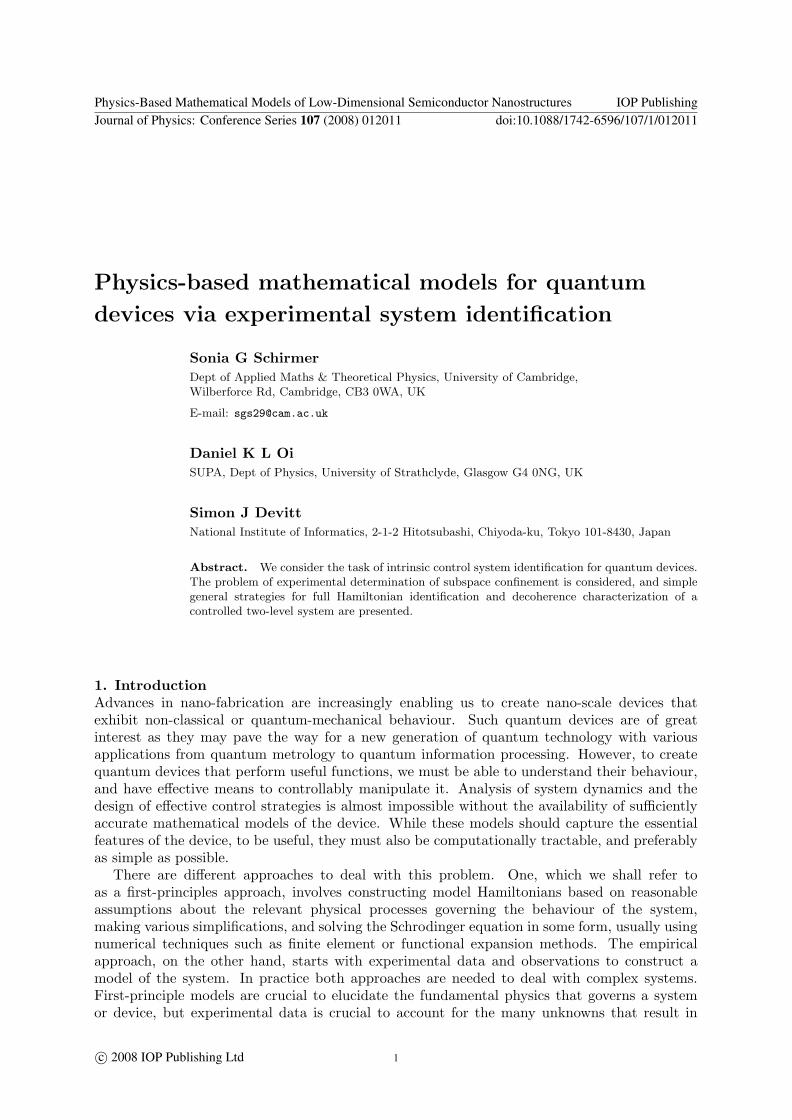
Figure 1 Simple charge lsquoqubitrsquo device Trench-isolated Silicon double quantum dot moleculefabricated using e-beam lithography controlled by several DC-gate electrodes with a singleelectron transistor for charge readout (Hitachi Cambridge Labs) (2)
variability of the characteristics of the system which is often difficult to predict or explaintheoretically For instance lsquomanufacturedrsquo systems such as artificial quantum dot lsquoatomsrsquo andlsquomoleculesrsquo vary considerably in size geometry internal structure etc and sometimes even smallvariations can significantly alter their behaviour
In this paper we will focus on constructing mathematical models solely from experimentaldata without any prior knowledge of the specifics of the system an approach one might callblack-box system identification We will restrict ourselves to quantum systems whose essentialfeatures can be captured by low-dimensional Hilbert space models For instance a quantumdot molecule such as the Silicon double quantum dot system in Fig 1 may consist of millionsof individual atoms with many degrees of freedom but the observable dynamics may be welldescribed by overall charge distribution states in the quantum dot molecule Taking these chargedistribution states as basis states for a Hilbert space H the observable dynamics of the systemis governed by a Hamiltonian operator acting on H and possibly additional non-Hermitianoperators to account for dissipative effects if the system is not completely isolated from itsenvironment If the dimension of the Hilbert space H is huge then complete characterizationof the Hamiltonian and dissipation operators may be a hopeless task but in certain cases thedynamics of interest takes place in low-dimensional Hilbert space H or we may in fact wish todesign a device whose dynamics can be described by a low-dimensional Hilbert space model asis the case in quantum information processing (1) where we desire to create systems that actas quantum bits for example
The paper is organized as follows We start with a general description of the basic assumptionswe make about the system to be modelled and the type of measurements and experiments uponwhich our characterization protocols are based In section 3 we discuss the problem of subspaceconfinement ie how to experimentally characterize how well the dynamics of system is confinedto a low-dimensional subspace such as a two-dimensional (qubit) Hilbert space In section 4 wepresent general protocols for identifying Hamiltonian and decoherence parameters for controlledqubit-like systems We conclude with a discussion of generalizations and open problems
2 General Modelling AssumptionsWe start with a generic model assuming only that the state of the system can be representedby a density operator (ie a positive operator of trace one) ρ acting on a Hilbert space H ofdimension N and that its evolution is governed by the quantum Liouville equation (in unitssuch that h = 1)
d
dtρ(t) = minusi[H ρ(t)] + LD[ρ(t)] (1)
Physics-Based Mathematical Models of Low-Dimensional Semiconductor Nanostructures IOP PublishingJournal of Physics Conference Series 107 (2008) 012011 doi1010881742-65961071012011
2
where H is an effective Hamiltonian and LD a super-operator that accounts for dissipative effectsdue to environmental influences etc Initially all that is known about H and LD is that His a Hermitian operator on H and LD a completely positive super-operator acting on densitymatrices ρ(t) although we may make some additional assumptions about the structure of Hor LD For instance we shall generally assumes LD to be of Kossakowski-Sudarshan-Lindbladform (3 4)
LD[ρ(t)] =N2minus1sumk=1
γkD[Vk]ρ(t) (2)
where the super-operators D[Vk] are defined by
D[A]B = ABAdagger minus (AdaggerAB + BAdaggerA)2 (3)
Vk are (generally non-Hermitian) operators on H and γk are positive real numbersIf the system is subject to dynamic control then the Hamiltonian (and sometimes the
relaxation operators Vk) are not fixed but dependent on external control fields which we shalldenote by f(t) In the simplest case we may assume a linear dependence of the Hamiltonian onthe controls
H[f(t)] = H0 +Msum
m=1
fm(t)Hm (4)
where the Hm are fixed Hermitian operators on H and the reservoir operators Vk are constantThe ultimate objective of characterization is to identify the operators H[f(t)] (or Hm) and
LD by performing suitable experiments on the system This task would be simplified if we couldassume that the system can be prepared in an arbitrary initial state ρ0 and that we can performgeneralized measurements or projective measurements in arbitrary bases at any timemdashbut theserequirements are generally unrealistic For example our ability to perform measurements on thesystem prior to characterization is limited by the direct readout processes available and often weonly have a single basic sensor such as a single electron transistor (SET) (5) providing relativelylimited information about the charge distribution in a quantum dot molecule or detection maybe accomplished via a readout transition that involves coupling one state of the system to afluorescent read-out state eg via a laser etc Furthermore preparation of non-trivial statesgenerally depends on knowledge of the operators H[f(t)] and LD the very information about thesystem we are trying to obtain These practical restrictions rule out conventional quantum stateor process tomography techniques which presume the ability to measure the system in differentmeasurement bases and prepare it in different initial states to obtain sufficient information toreconstruct the quantum state or process (6 7 8 9 10)
In this paper we consider a rather typical experimental scenario where we are limited tomeasurements of a fixed observable and evolution under a Hamiltonian that can be modified byvarying certain control settings For the most part we restrict ourselves further to piecewiseconstant controls The only assumption on the measurement process we make is that it canbe formally represented by some Hermitian operator A with N eigenvalues corresponding tomeasurement outcomes λn ie that it has a spectral decomposition of the form
A =Nsum
n=1
λn|n〉〈n| (5)
This measurement also serves as initialization of the system as outcome λn means that the systemwill be left in an eigenstate |n〉 associated with the eigenvalue λn If A has N unique eigenvaluesie all eigenvalues occur with multiplicity one then the measurement is sufficient to initialize
Physics-Based Mathematical Models of Low-Dimensional Semiconductor Nanostructures IOP PublishingJournal of Physics Conference Series 107 (2008) 012011 doi1010881742-65961071012011
3
the system in a unique state if it has degenerate eigenvalues associated with eigenspaces ofdimension greater gt 1 then some measurement outcomes will not determine the state uniquely
Following the idea of intrinsic characterization our objective is to extract informationabout the system without recourse to any external resources ie using no information frommeasurements other than the information provided by the sensors built into the device and noexternal control fields except the ability to change the settings of the built-in actuators (suchas variable gate voltages) subject to constraints Although this requirement of characterizationrelying only on the built-in sensors and actuators may seem excessively restrictive excludingmany forms of spectroscopy for example it has the advantage of simplicity (no externalresources required) Moreover external sensors and actuators may disturb the system andthus characterization of the system in their presence may not yield an accurate picture of thedynamics in the absence of the additional apparatus
We restrict ourselves here to systems sufficiently weakly coupled to a sufficiently largereservoir whose dynamics can be described by adding a dissipation super-operator of the form (2)to the Hamiltonian dynamics of the subsystem of interest Although many systems can bemodelled this way it should be noted that this approach has limitations For example thedynamics of a subsystem HS that is strongly is coupled to a finite reservoir HR such as singlespin coupled to several nearby spins can be very complicated and non-Markovian Althoughnon-Markovian dynamics can in principle be dealt with by allowing time-dependent relaxationoperators Vk in such cases it is not always possible to describe the dynamics of the subsystemof interest in terms of the Hamiltonian dynamics on the subspace and a set of simple relaxationor decoherence operators Rather it may become necessary to consider the system HS + HR
and characterize its dynamics described by a Schrodinger equation with a Hamiltonian HS+Rinstead to obtain an accurate picture of the subsystem dynamics The basic ideas of intrinsiccharacterization can be applied to this larger system and the protocols we will describe can inprinciple be extended to such higher-dimensional systems although full characterization of thesystem plus reservoir Hamiltonian HS+R using only the built-in sensors and actuators may notbe possible The degree of characterization possible will depend on the size of the Hilbert spaceand the capabilities of the built-in sensors and actuators eg to discriminate and manipulatedifferent states of the larger system Before attempting to identify the system Hamiltonian (anddecoherence operators) an important first task is therefore estimating the dimension of theHilbert space in which the dynamics takes place
3 Characterization of subspace confinementA fundamental prerequisite for constructing a Hilbert space model is knowledge of the underlyingHilbert space This is a nontrivial problem as most systems have many degrees of freedom andthus a potentially huge Hilbert space but effective characterization of the system often dependson finding a low dimensional Hilbert space model that captures the essential features of thesystem Furthermore in applications such as quantum information processing the elementarybuilding blocks are required to have a certain Hilbert space dimension For example for aquantum-dot molecule to qualify as a qubit we must be able to isolate a two-dimensionalsubspace of the total Hilbert space and be able to coherently manipulate states within this2D subspace without coupling to states outside the subspace (leakage) This requires severalcharacterization steps
(i) Isolation of a 2D subspace and characterization of subspace confinement(ii) Characterization of the Hamiltonian dynamics including effect of the actuators and(iii) Characterization of (non-controllable) environmental effects (dissipation)
The choice of a suitable subspace depends also on the measurement device as the measurementmust be able to distinguish the basis states Thus for a potential charge qubit device for example
Physics-Based Mathematical Models of Low-Dimensional Semiconductor Nanostructures IOP PublishingJournal of Physics Conference Series 107 (2008) 012011 doi1010881742-65961071012011
4
0 10 20 30 40 50 60 70 80 90 100
0
001
002
003
evolution time t
1minusT
r[Π ρ
(t)]
calculatedestimated
Figure 2 Leakage characterization assuming three-outcome measurement for system initializedin state |0〉 The continuous curve is the calculated value of pleak(t) = 1 minus Tr[Πρ(t)] whereΠ = |0〉〈0| + |1〉〈1| is the projector onto the target subspace for a 10-level test HamiltonianThe red dots are the estimates of pleak(t) at the discrete times tk = (k minus 1)∆t with ∆t = 001obtained by averaging over N prime
e = 100 simulated experiments for each tk As the figure showsthe effect of the projection noise makes it difficult to obtain accurate estimates of pleak(t) forany given t = tk unless N prime
e is extremely large However the average leakage rate over the timeinterval [0 100] pleak = 011 for both the calculated and measured values
only a subspace spanned by charge states that can be reliably distinguished by the SET is asuitable candidate and ideally there should be two (or in general N) orthogonal states thatcan be perfectly distinguished by the measurement so that we have a well-defined referenceframe (basis) |0〉 |1〉 |N〉 and the measurement can be represented by an observable ofthe form (5) with N distinct eigenvalues λn Furthermore we would like the readout processto act as a projective measurement so that each measurement projects the state of the systemonto one of the measurement basis states |n〉 The ability to perform projective measurementsis not a trivial requirement especially for solid state systems and is not an absolute necessity ascharacterization protocols can be adapted to weak measurements but projective measurementscan in principle be achieved with various sensors such as rf-SETs and we shall assume here thatwe are working in this regime
After a possible subspace has been identified it is crucial to check that the subspace issufficiently isolated ie that we can reliably initialize the system in a state in this subspace andthat it remains in this subspace under both free and controlled evolution This characterizationof subspace confinement is very important If the device is a candidate for a qubit for exampleit is essential that subspace leakage be much less than the rate of bit or phase flip errors due toimperfect control or decoherence as leakage or loss error correction protocols are considerablymore demanding in terms of complexity and resources required
Characterization of subspace confinement depends on the characteristics of the sensors iethe type of measurements we can perform For our charge qubit with SET readout example ifthe SET can be calibrated to be sufficiently sensitive to enable detection of states outside thechosen subspace in addition to being able to discriminate the subspace basis states |n〉 ie if thetrue measurement has (at least) N + 1 mutually exclusive outcomes λn n = 1 N and λN+1
if the system state is outside the subspace then the characterization of subspace confinement isrelatively easy If we perform Ne experiments of the form
(i) Initialize Measure and record outcome λa
(ii) Evolve Let the system evolve for time t under some fixed Hamiltonian Hf
Physics-Based Mathematical Models of Low-Dimensional Semiconductor Nanostructures IOP PublishingJournal of Physics Conference Series 107 (2008) 012011 doi1010881742-65961071012011
5
minus10 minus8 minus6 minus4 minus2 0 2 4 6 8 100
02
04
frequency ω
Re(
FT
[p0] )
02468 02468
05035
Ne=100 ∆ t=001
0 10 20 30 40 50 60 70 80 90 1000
05
1
t (arb units)
p 0(t)
Figure 3 p0(t) obtained by averaging over Ne = 100 simulated experiments with a 10-level testHamiltonian and corresponding Fourier spectrum From the 0th and 1st order peak heights weobtain h0 +2h1 = 09970 which yields upper and lower bounds for ε of asymp 00015 although thesebounds are statistically uncertain due to projection noise and discretization errors Nonethelessit can be verified that the actual subspace confinement for the chosen test Hamiltonian is 9994and thus the upper bound provides a reasonable estimate for the leakage
(iii) Measure Repeat measurement and record outcome λb
and denote by Nab the number of times the measurement results for the initial and finalmeasurements were λa and λb respectively then for Ne sufficiently large the leakage out of thesubspace is approximately equal to the fraction of experiments for which the first measurementwas λn with n le N and the second measurement was N + 1 ie
pleak asympsumN
n=1 NnN+1
Ne minussumN+1
n=1 NN+1n
(6)
Repeating the experiments for different evolution times t and averaging then gives an indicationof the rate of subspace leakage eg if we estimate pleak(tk) for tk = k∆t k = 0 K then
pleak =1
tmax
int tmax
0pleak(t) dt asymp 1
K + 1
Ksumk=0
pleak(tk) (7)
If the SET (or other measurement process) is not sufficiently sensitive to reliably distinguishat least N subspace basis states |n〉 as well as states outside the subspace then subspacecharacterization is more challenging For instance suppose we have a 2D subspace and asensor that can reliably detect only one state say |0〉 a common scenario for many systemswhere readout transitions are used that detect only a single state In this case the measurementoutcomes are λ0 or notλ0 If the measurement is projective and the dynamics confined to a 2Dsubspace we can identify notλ0 with outcome λ1 but this identification will lead to errors ifthe dynamics is not really confined to a 2D subspace However even in this case we can stillestimate the level of confinement to a 2D subspace under the evolution of a Hamiltonian Hf
Physics-Based Mathematical Models of Low-Dimensional Semiconductor Nanostructures IOP PublishingJournal of Physics Conference Series 107 (2008) 012011 doi1010881742-65961071012011
6
from observable coherent oscillations For example let
p0(t) = |〈0|eminusiHf t|0〉|2 (8)
be the probability of obtaining outcome λ0 when measuring the time-evolved state |Ψ(t)〉 =exp(minusitHf )|0〉 If the system is initialized in the state |0〉 and the dynamics of the system underHf is perfectly confined to a two-level subspace then conservation of probability implies that theheights h0 and h1 of the 0th and 1st order terms in the Fourier spectrum of p0(t) must satisfyh0 +2h1 = 1 We can use the deviation from this equality to bound the subspace leakage ε (11)
1minusradic
h0 + 2h1 le ε le 12(1minus
radic2(h0 + 2h1)minus 1) (9)
As the upper and lower bounds depend only on the 0th and 1st order Fourier peaks theycan usually be easily determined from experimental data although finite resolution due todiscretization and projection noise will reduce the accuracy of the estimates (11) Moreoverin this case 1minus ε only indicates the confinement of the system to some two-level subspace andwe must be careful as for different controls f the dynamics under Hf may be confined to differenttwo-level subspaces in which case the system cannot be considered a proper qubit For instancefor the 10-level test Hamiltonian
Htest =
13701 10000 00093 00055 00112 00068 00119 00084 00065 0008710000 15561 00109 00132 00067 00061 00081 00051 00105 0002900093 00109 16603 00034 00161 00100 00101 00123 00115 0005500055 00132 00034 19112 00136 00072 00093 00062 00133 0010100112 00067 00161 00136 34611 00022 00119 00078 00064 0012200068 00061 00100 00072 00022 43017 00074 00077 00029 0008000119 00081 00101 00093 00119 00074 68732 00133 00158 0015400084 00051 00123 00062 00078 00077 00133 73491 00071 0007300065 00105 00115 00133 00064 00029 00158 00071 81876 0010800087 00029 00055 00101 00122 00080 00154 00073 00108 89032
used for the simulated experiments in Figs 2 and 3 the first procedure measures the projectiononto the subspace S1 spanned by the measurement basis states |0〉 = (1 0 0 0 0 0 0 0 0 0 0)T
and |1〉 = (0 1 0 0 0 0 0 0 0 0 0)T while the second procedure measures the confinement ofthe dynamics to the best-fitting 2D subspace S2 which for the given Hamiltonian is spanned by
v1 = (1minus00001 00004 00034minus00012minus00002minus00005minus00004 00003minus00005)T
v2 = (0 1 00174 00238minus00131minus00051minus00032minus00020minus00022minus00013)T
and comparison of the results confirms that the average confinement 1minus pleak for the subspaceS1 as obtained by the first procedure is less (9989) than the confinement for subspace S2
(9994)
4 General characterization protocols for qubit systemsOnce a suitable subspace has been chosen we can proceed to the second stage of thecharacterization identification of the Hamiltonian and decoherence operators The simplesttype of system we can consider here is a qubit with Hilbert space dimension 2 In this case anynon-trivial projective measurement ie any measurement with two distinguishable outcomesλ0 and λ1 can be represented by an observable A = λ0|0〉〈0|+ λ1|1〉〈1| The eigenstates |0〉 and
Physics-Based Mathematical Models of Low-Dimensional Semiconductor Nanostructures IOP PublishingJournal of Physics Conference Series 107 (2008) 012011 doi1010881742-65961071012011
7
(a) (b)
Figure 4 Bloch sphere representation of dynamics (a) Arrangement of rotation axes dk withrespect to reference rotation axis dr (b) The evolution of the vector s(t) with s0 = (0 0 1)T
about the axis d and the projection of s(t) onto the z-axis
|1〉 of A define a basis for the Hilbert space and we can define the Pauli operators σ0 σx σy
and σz with respect to this basis
σ0 = |0〉〈0|+ |1〉〈1| σz = |0〉〈0| minus |1〉〈1| (10a)σx = |0〉〈1|+ |1〉〈0| σy = i(minus|0〉〈1|+ |1〉〈0|) (10b)
or in the usual matrix notation
σ0 =(
1 00 1
) σx =
(0 11 0
) σy =
(0 minusii 0
) σz =
(1 00 minus1
) (11)
Taking (without loss of generality) the measurement outcomes to be λ0 = 1 and λ1 = minus1 wehave A = σz in this basis Furthermore we can expand any Hamiltonian of the system as
H =12(d0σ0 + dxσx + dyσy + dzσz) (12a)
=d0
2σ0 +
ω
2(sin θ cos φ σx + sin θ sinφ σy + cos θ σz) (12b)
The d0 term can generally be ignored as the identity σ0 commutes with all other Pauli matricesand exp(minusitd0σ0) corresponds to multiplication by a global phase factor ie trivial dynamicsHence it suffices to determine the real vector d = (dx dy dz) or in polar form the angles(ω θ φ) to determine the Hamiltonian For a single Hamiltonian we can furthermore choosethe coordinate system such that φ = 0 However since H depends on control inputs f theparameters ω θ and φ also depend on the controls f and we usually need to determine Hf formany different f In this case we can choose a reference Hamiltonian eg Href with φ = 0 butwe must determine the relative angles φ with respect to the reference Hamiltonian for all othercontrol settings
41 Rotation frequency and declination of rotation axisTo relate the Hamiltonian parameters to observable dynamics it is instructive to visualize qubitstates and their evolution on the Bloch sphere If we define s = (sx sy sz)T with sk = Tr(ρσk)
Physics-Based Mathematical Models of Low-Dimensional Semiconductor Nanostructures IOP PublishingJournal of Physics Conference Series 107 (2008) 012011 doi1010881742-65961071012011
8
for k isin x y z then it is easy to check that there is a one-to-one correspondence betweendensity operators ρ and points s inside the closed unit Ball in IR3 Furthermore the evolutionof ρ(t) under the (constant) Hamiltonian (12) corresponds to a rotation of s(t) about the (unit)axis d = (sin θ cos φ sin θ sinφ cos θ)T with angular velocity ω as illustrated in Fig 4 Thefigure also shows that we can determine the angle θ and angular frequency d = ω from theprojection of s(t) under the rotation about the axis d onto the z-axis As the figure shows givenz(t) we can in principle extract ω and θ from the first minimum (t0 z0) of z(t) although inpractice it is usually preferable to use Fourier analysis or harmonic inversion techniques z(t)being the expectation value 〈A(t)〉 = Tr[σzρ(t)] of the observable A = σz in the state ρ(t) canbe obtained experimentally as follows (12)
(i) Initialize Measure and record outcome λa = plusmn1 rArr system in state λas0 = λa(0 0 1)T (ii) Evolve Let the system evolve for time t under the control settings f rArr system now in
state λas(t) = λa(x(t) y(t) z(t))T with
z(t) = cos2 θ + sin2 θ cos(ωt) (13)
(iii) Measure Repeat measurement and record outcome λb = plusmn1 rArr system now in state λbs0(iv) Repeat steps (i)ndash(iii) Ne times
Let Nab be the number of times the the initial measurement produced outcome λa and the finalmeasurement produced outcome λb Then there are four possible combinations of outcomesN00 N01 N10 and N11 which must add to the total number of experiments Ne The numberof experiments that started in the state |0〉 [or s0 = (0 0 1)T ] is N prime
e = N00 + N01 and thefraction of experiments for which the second measurement yields λ0 conditioned on the systemstarting in the state |0〉 is N00N
primee Thus the ensemble average of A = σz at time t assuming
we started in the state |0〉 is
λ0N00
N primee
+ λ1N01
N primee
=λ0N00 + λ1N01
N00 + N01 (14)
and for Ne rarr infin this relative frequency should approach the true expectation value of z(t)assuming z(0) = 1 Thus we can in principle determine z(t) to arbitrary accuracy by choosingNe large enough By repeating the experiments for different evolution times tk eg using astroboscopic mapping approach (see Fig 5) we can determine z(t) as a function of t from whichwe can extract ω = ωf and θ = θf as discussed For instance noting that z(t) = 2p0(t)minus1 Fig 3shows that the 1st order Fourier peak F (ω) of z(t) in this example is F (ω) asymp 2times02468 = 04935for ω asymp 2 and thus comparison with Eq (13) shows that sin2 θ = 2lt[F (ω)] or equivalentlyθ asymp 14566 These values are reasonably good estimates for the real values ω = 20086 andθ = minus14780 except for the sign of θ or the orientation of the rotation axis which we cannotdetermine from the given data as these rotations have identical projections onto the z-axisThis is reflected in Eq (13) by the fact that both coefficients cos2 θ and sin2 θ contain squaresIn principle we can determine the parameters ω and θ to arbitrary accuracy using this approachbased on regular sampling and Fourier analysis (13) although the total number of experimentscan become prohibitively large An alternative that merits further investigation is the use ofadaptive sampling techniques to reduce the total number of experiments necessary
42 Relative angles between rotation axesHaving determined the parameters ωf and θf for a particular control setting f and chosen asuitable reference Hamiltonian Href with φref = 0 to complete the characterization of Hf 6= Href we must determine the horizontal angle φf The reference Hamiltonian Href must not commute
Physics-Based Mathematical Models of Low-Dimensional Semiconductor Nanostructures IOP PublishingJournal of Physics Conference Series 107 (2008) 012011 doi1010881742-65961071012011
9
Init
Init
Init
Init
Meas
Meas
Meas
Meas
minus1
+1
z(t) = 〈σz〉
H(2∆t)
H(4∆t)
H(3∆t)
H(∆t)
Figure 5 Stroboscopic mapping of coherent oscillations with projective measurements Afterinitialization through measurement the system is allowed to evolve for fixed times under theinfluence of the controls before a second measurement is taken The experiments are repeatedto determine the expectation value of the observable at each time
with the measured observable A or equivalently the angle θref between the rotation axis dref
and the z-axis must be nonzero Ideally dref should be as close to orthogonal to the z-axis aspossible Assuming θref isin (π4 π2] and ωf and θf are known we can determine the angles φf
by performing the following experiments (12)
(i) Initialize Measure and record outcome λa = plusmn1 rArr system in state λas0 = λa(0 0 1)T (ii) Prepare Rotate around reference axis dref by angle α0 = arccos(1minusx
1+x) x = minus cos(2θref)rArr system in new state λas1 = λa(cos β sinβ 0)T with β = arctan(minus
radic2x) cos θref
(iii) Evolve Let the system evolve for time t under the control settings f rArr system in newstate λas(t) = λa(x(t) y(t) z(t))T with
z(t) = c[1minus cos(ωf t)] + d sin(ωf t) (15a)c = sin θf cos θf cos(φf minus β) (15b)d = sin θf sin(φf minus β) (15c)
(iv) Measure Repeat measurement and record outcome λb = plusmn1 rArr system in new state λbs0(v) Repeat steps (i)ndash(iv) Ne times
As before if Nab is the number of times the initial measurement produced outcome λa and thefinal measurement produced outcome λb then we have
z(t) asymp λ0N00 + λ1N01
N00 + N01
for sufficiently large Ne thus allowing us to determine z(t) experimentally Since θf ωf and β areknown from the θ ω characterization step Eq (15) allows us to determine φf via the coefficientsc and d which can be determined in principle either through curve fitting or by taking theFourier transform of z(t) and noting that c and d correspond to the real and imaginary part ofthe 0th and 1st order Fourier peaks
As a specific example assume we have two Hamiltonians H1 and H2 and we have alreadydetermined ω1 = 1 θ1 = π
4 and ω2 = 12 θ2 = π6 We choose H1 as reference Hamiltonian and
Physics-Based Mathematical Models of Low-Dimensional Semiconductor Nanostructures IOP PublishingJournal of Physics Conference Series 107 (2008) 012011 doi1010881742-65961071012011
10
0 10 20 30 40 50 60 70 80 90 100
minus05
0
05
1
evolution time t
z(t)
Ne=100 dt=001
minus15 minus1 minus05 0 05 1 15minus04
minus02
0
02
04
angular frequency ω
FT
(z) 0304466
Figure 6 Determination of relative horizontal angle between two Hamiltonians Measuredprojection z(t) of s1(t) onto the z-axis and corresponding Fourier spectrum Blueredbars indicate the cosinesine coefficients ie realimaginary parts of the Fourier transformrespectively
note that a rotation about H1 by α = π maps the state s0 = (0 0 1)T to s1 = (1 0 0)T Wethen let state s1 evolve for different length of time t under Hamiltonian H2 and determine theprojection z(t) This will produce a measured z-trace as shown in Fig 6 Eq (15) shows thatin theory the height of the real part of the 0th and 1st order Fourier peaks should be the sameexcept for the sign but the graph clearly shows that this is not the case for our noisy (simulated)experimental data In fact the 1st order peaks around plusmnωf are significantly broadened whilethe 0-peak is very narrow This suggests that we are likely to obtain the best estimate for φby setting c = FT[z](0) and φf = arccos[c(sin θf cos θf )] + β where β = 0 in our case Indeedthis yields an estimate of φf = 02518π which is very close to actual value π4 used in thesimulation Note that using the 1st order Fourier peaks gives far less accurate results due tothe significant broadening of the peaks This can be reduced using phase matching conditionsand other tricks (13) but in this case simply using only the 0-peak is sufficient to get a goodestimate
43 Functional dependence on control settingsIn some settings it is sufficient to characterize the Hamiltonians Hf for a discrete finite setof controls f (k) This would be the case for bang-bang-type control schemes that requireonly switching between a finite set of control Hamiltonians In other cases in particularwhen continuously varying fields are to be applied we would also like to know the functionaldependence of the Hamiltonian on the control fields eg whether we can assume a control-linearmodel as in (4) or if there are non-linear or crosstalk effects etc Although characterizing thecontrol dependence of the Hamiltonian is a non-trivial problem given sufficiently many Hf datapoints it is possible to test the quality of fit of a particular model using statistical means Forinstance suppose we have characterized the Hamiltonians Hf for f isin f (k) Let dk be thecorresponding vectors in IR3 as defined above and let f
(k)m be the mth component of the control
vector f (k) We can find the best-fitting linear model by finding vectors dm isin IR3 m = 0 M
Physics-Based Mathematical Models of Low-Dimensional Semiconductor Nanostructures IOP PublishingJournal of Physics Conference Series 107 (2008) 012011 doi1010881742-65961071012011
11
0 02 04 06 08 1 12 14 16 180
2
4
control input f (arb units)
x z
com
p o
f rot
axi
s
dx(f)
dz(f)
dz=1002minus0003f ∆=0013
dx=0006f+0996f2 ∆=0016
0 10 20 30 40 50 60 70 80 90 100
08
1
evolution time t
z(t)
Ne=100 dt=001 f=06
Figure 7 Determination of functional dependence of Hf on control input f The bottom graphshows the estimated values for d
(k)x and d
(k)z (circles and triangles respectively) as well as the
actual functional dependence in the model (solid lines) The top graph shows a typical z(t)trace obtained by averaging over Ne = 100 simulated experiments for each time tk = 001k Theeffects of finite sampling and projection noise are clearly visible for this trace Nonetheless thepredicted functional dependence of Hf on the control input f is in good agreement with theactual dependence in the model
where M is the number of independent control variables that minimize the norm of the residuals
∆ =radicsum
k rk22 where
rk = d0 +Msum
m=1
f (k)m dm minus dk (16)
The norm of the residuals ∆ then gives an indication of the quality of fit of a linear dependencemodel and allows us to compare the quality of fit for different models
As an example consider a Hamiltonian Hf depending on a one-dimensional control inputf = f To characterize the functional dependence of Hf on f we choose a finite set of controlsettings fk = 02(k minus 1) for k = 1 10 We characterize first the rotation frequencies ωk
and declination angles θk for each fk and then the relative angles φk as discussed above Fromthese we calculate the components d
(k)x d
(k)y and d
(k)z of the Hamiltonian according to Eq (12)
and plot them versus f as shown in Fig 7 Specifically in our case we find φk asymp 0 and hencedy equiv 0 dz appears to be constant and dx exhibits a quadratic dependence on the control f A least square fit of the data using a linear and quadratic fitting function respectively yieldsdz(f) = 1002 minus 0003 f and dx(t) = 0006f + 0996f2 which is in very good agreement withthe actual functional dependence in the model dz(f) = 1 and dx(f) = f2 despite the fact thatthe simulated data appears very noisy and the θ and ω estimates did not employ tuning such asphase matching to further improve the accuracy
44 Characterization in the presence of decoherenceThe protocols for Hamiltonian identification above are sufficient if dissipative effects are small onthe timescales for coherent control ie if the system and environment coupling is much weaker
Physics-Based Mathematical Models of Low-Dimensional Semiconductor Nanostructures IOP PublishingJournal of Physics Conference Series 107 (2008) 012011 doi1010881742-65961071012011
12
than the system-control interaction If the coupling between the system and its environment isstronger then dissipative effects must be directly incorporated into the characterization protocols
Assuming Markovian decoherence of the form (2) it is easy to show that for N = 2 wehave Ak = U σkU
dagger where σk are the elementary relaxation operators σminus σ+ 12 σz defined
in terms of the Pauli matrices σplusmn = 12(σx ∓ iσy) and U is some unitary operator in SU(2)
that defines a preferred decoherence basis The operator σz is usually associated with puredecoherence (pure dephasing) while the raising and lowering operators σplusmn are associated withpopulation relaxation from |1〉 to |0〉 and vice versa Very often it is furthermore assumed thatU = I is the identity ie that the preferred basis for relaxation is the same as the measurementbasis Although this need not be the case it is often a good approximation The main effectof relaxation processes is to dampen the observed coherent oscillations z(t) that result from theHamiltonian dynamics and try to force the system lsquoasymptoticallyrsquo into a lsquosteadyrsquo state Thiseffect manifests itself in Lorentzian broadening of the peaks in the oscillation spectrum whichcan be used for characterization purposes
For example Fig 8 shows significantly damped oscillations as a result of relaxation The factthat the oscillations decay to zinfin = 0 suggests either pure dephasing or a symmetric relaxationprocess with Γ+ = Γminus ie equal probability of relaxation from state |0〉 to |1〉 and vice versaor a combination of both Since symmetric relaxation and pure dephasing have very similarsignatures it can be difficult to distinguish these processes from the oscillation trace aloneHowever if there exists a control f such that Hf prop σz which corresponds to a rotation aboutthe z (or measurement) axis then we can in principle distinguish the two processes by initializingthe system repeatedly in either state |0〉 or |1〉 and letting the system evolve under Hf for variousperiods of time before measuring again If the decoherence process is pure dephasing then thesystem will remain in the initial state while we expect to observe random jumps (with equalprobability) for symmetric relaxation Assuming this preliminary characterization step suggeststhat the damping in the figure is due to pure dephasing we can then extract information aboutthe rotation frequency ω0 and dephasing rate Γ by fitting a Lorentzian envelope function
Lω0Γ(ω) =Γ
(ω minus ω0)2 + Γ2(17)
to the first-order peak in the Fourier spectrum as shown in the figure In our example usinga simple least-squares minimization yields estimated values for both ω0 and Γ that are close tothe actual values used in the simulated experiment This approach can be generalized for morecomplicated relaxation processes (14) Alternatively if we can characterize the Hamiltoniandynamics sufficiently to be able to initialize the system in non-measurement basis states andsimulate readout in different bases then generalized Lindblad operators can be estimated usingrepeated process tomography (15)
5 Discussion of generalizations and conclusionsWe have described some basic tools and techniques for characterizing the extent to whichthe dynamics of a certain system is confined to a low-dimensional subspace of a potentiallylarge Hilbert space as well as for identifying both Hamiltonian and decoherence parametersexperimentally with emphasis on protocols that are realistic even in the presence of limiteddirect readout and control capabilities
Although the explicit schemes presented focused on qubit-like systems the same basic ideascan be applied to higher-dimensional systems However the number of Hamiltonian anddecoherence parameters to be determined for higher-dimensional system makes finding explicitprotocols for complete characterization quite challenging The qubit characterization protocolsshow that identifying the relative angles between several control Hamiltonians requires a two-stage process and more complicated two-step experiments (initialization in non-measurement
Physics-Based Mathematical Models of Low-Dimensional Semiconductor Nanostructures IOP PublishingJournal of Physics Conference Series 107 (2008) 012011 doi1010881742-65961071012011
13
0 10 20 30 40 50 60 70 80 90 1000
05
1
evolution time t
z(t)
ω0=1414
Γ=01
minus15 minus1 minus05 0 05 1 150
002
004
006
angular frequency ω
Re[
FT
(z)]
ω
0est=1406
Γest
=009703Re FT[z]
Lorentzian fit
Figure 8 Characterization in the presence of decoherence The observed damped oscillationsdue to pure dephasing (top) result in Lorentzian broadening of the Fourier peaks which can beexploited to obtain (good) estimates for the rotation frequency ω0 and decoherence rate Γ
basis state followed by controlled evolution) than identifying the rotation frequency anddeclination angle for a single Hamiltonian As the dimension of the system increases moreparameters are necessary to fully characterize the Hamiltonians leading to more complex multi-stage characterization protocols
Another problem is that the number of experiments required to implement such schemesmay become prohibitively large for parameter estimation based on spectroscopic analysis Oneof the most promising strategies to avoid this problem is the development of efficient adaptivecharacterization schemesmdashas opposed to protocols based on regular samplingmdash to minimize thenumber of measurements experiments required For systems composed of separate smaller unitssuch as multi-qubit systems boot-strapping approaches to characterization may also provide afruitful alternative For example assuming we have separately characterized individual qubitsusing qubit identification protocols and therefore have full local control we can reduce theproblem of two-qubit identification in principle to identifying the interaction Hamiltonian Fortwo-qubit systems with local control and a fully non-local interaction Hamiltonian this can beachieved using entanglement mapping or concurrence spectroscopy (16 17)
AcknowledgmentsSGS acknowledges funding from an EPSRC Advanced Research Fellowship and support fromHitachi and the EPSRC QIP IRC DKLO is supported by a SUPA fellowship SJD acknowledgessupport from MEXT
References[1] Nielsen M A and Chuang I L 2000 Quantum Computation and Quantum Information
(Cambridge UK Cambridge University Press)[2] Gorman J Hasko D G and Williams D A 2005 Phys Rev Lett 95 090502[3] Lindblad G 1976 Comm Math Phys 48 119ndash130[4] Gorini V Kossakowski A and Sudarshan E C G 1976 J Math Phys 17 821ndash825
Physics-Based Mathematical Models of Low-Dimensional Semiconductor Nanostructures IOP PublishingJournal of Physics Conference Series 107 (2008) 012011 doi1010881742-65961071012011
14
[5] Devoret M H and Schoelkopf R J 2000 Nature 406 1039[6] Chuang I L and Nielson M A 1997 J Mod Opt 44 2455[7] Poyatos J F Cirac J I and Zoller P 1997 Phys Rev Lett 78 0390[8] Leung D W 2003 J Math Phys 44 0528[9] Thew R T Nemoto K White A G and Munro W J 2002 Phys Rev A 66 012303
[10] Kosut R Walmsley I A and Rabitz H 2004 Optimal experiment design for quantum stateand progress tomography and Hamiltonian parameter estimation quant-ph0411093
[11] Devitt S J Schirmer S G Oi D K L Cole J H and Hollenberg L C L 2007 New J Physics7 384
[12] Schirmer S G Kolli A and Oi D K L 2004 Phys Rev A 69 050603(R)[13] Cole J H Schirmer S G Greentree A D Wellard C J Oi D K L and Hollenberg L C L 2005
Phys Rev A 71 062312[14] Cole J H Greentree A D Oi D K L Schirmer S G Wellard C J and Hollenberg L C L 2006
Phys Rev A 73 062333[15] Boulant N Havel T F Pravia M A and Cory D G 2003 Phys Rev A 67 042322[16] Devitt S J Cole J H and Hollenberg L C L 2006 Phys Rev A 73 052317[17] Cole J Devitt S and Hollenberg L 2006 J Phys A 39 14649ndash14658
Physics-Based Mathematical Models of Low-Dimensional Semiconductor Nanostructures IOP PublishingJournal of Physics Conference Series 107 (2008) 012011 doi1010881742-65961071012011
15
Physics-based mathematical models for quantum
devices via experimental system identification
Sonia G SchirmerDept of Applied Maths amp Theoretical Physics University of CambridgeWilberforce Rd Cambridge CB3 0WA UK
E-mail sgs29camacuk
Daniel K L OiSUPA Dept of Physics University of Strathclyde Glasgow G4 0NG UK
Simon J DevittNational Institute of Informatics 2-1-2 Hitotsubashi Chiyoda-ku Tokyo 101-8430 Japan
Abstract We consider the task of intrinsic control system identification for quantum devicesThe problem of experimental determination of subspace confinement is considered and simplegeneral strategies for full Hamiltonian identification and decoherence characterization of acontrolled two-level system are presented
1 IntroductionAdvances in nano-fabrication are increasingly enabling us to create nano-scale devices thatexhibit non-classical or quantum-mechanical behaviour Such quantum devices are of greatinterest as they may pave the way for a new generation of quantum technology with variousapplications from quantum metrology to quantum information processing However to createquantum devices that perform useful functions we must be able to understand their behaviourand have effective means to controllably manipulate it Analysis of system dynamics and thedesign of effective control strategies is almost impossible without the availability of sufficientlyaccurate mathematical models of the device While these models should capture the essentialfeatures of the device to be useful they must also be computationally tractable and preferablyas simple as possible
There are different approaches to deal with this problem One which we shall refer toas a first-principles approach involves constructing model Hamiltonians based on reasonableassumptions about the relevant physical processes governing the behaviour of the systemmaking various simplifications and solving the Schrodinger equation in some form usually usingnumerical techniques such as finite element or functional expansion methods The empiricalapproach on the other hand starts with experimental data and observations to construct amodel of the system In practice both approaches are needed to deal with complex systemsFirst-principle models are crucial to elucidate the fundamental physics that governs a systemor device but experimental data is crucial to account for the many unknowns that result in
Physics-Based Mathematical Models of Low-Dimensional Semiconductor Nanostructures IOP PublishingJournal of Physics Conference Series 107 (2008) 012011 doi1010881742-65961071012011
ccopy 2008 IOP Publishing Ltd 1
Figure 1 Simple charge lsquoqubitrsquo device Trench-isolated Silicon double quantum dot moleculefabricated using e-beam lithography controlled by several DC-gate electrodes with a singleelectron transistor for charge readout (Hitachi Cambridge Labs) (2)
variability of the characteristics of the system which is often difficult to predict or explaintheoretically For instance lsquomanufacturedrsquo systems such as artificial quantum dot lsquoatomsrsquo andlsquomoleculesrsquo vary considerably in size geometry internal structure etc and sometimes even smallvariations can significantly alter their behaviour
In this paper we will focus on constructing mathematical models solely from experimentaldata without any prior knowledge of the specifics of the system an approach one might callblack-box system identification We will restrict ourselves to quantum systems whose essentialfeatures can be captured by low-dimensional Hilbert space models For instance a quantumdot molecule such as the Silicon double quantum dot system in Fig 1 may consist of millionsof individual atoms with many degrees of freedom but the observable dynamics may be welldescribed by overall charge distribution states in the quantum dot molecule Taking these chargedistribution states as basis states for a Hilbert space H the observable dynamics of the systemis governed by a Hamiltonian operator acting on H and possibly additional non-Hermitianoperators to account for dissipative effects if the system is not completely isolated from itsenvironment If the dimension of the Hilbert space H is huge then complete characterizationof the Hamiltonian and dissipation operators may be a hopeless task but in certain cases thedynamics of interest takes place in low-dimensional Hilbert space H or we may in fact wish todesign a device whose dynamics can be described by a low-dimensional Hilbert space model asis the case in quantum information processing (1) where we desire to create systems that actas quantum bits for example
The paper is organized as follows We start with a general description of the basic assumptionswe make about the system to be modelled and the type of measurements and experiments uponwhich our characterization protocols are based In section 3 we discuss the problem of subspaceconfinement ie how to experimentally characterize how well the dynamics of system is confinedto a low-dimensional subspace such as a two-dimensional (qubit) Hilbert space In section 4 wepresent general protocols for identifying Hamiltonian and decoherence parameters for controlledqubit-like systems We conclude with a discussion of generalizations and open problems
2 General Modelling AssumptionsWe start with a generic model assuming only that the state of the system can be representedby a density operator (ie a positive operator of trace one) ρ acting on a Hilbert space H ofdimension N and that its evolution is governed by the quantum Liouville equation (in unitssuch that h = 1)
d
dtρ(t) = minusi[H ρ(t)] + LD[ρ(t)] (1)
Physics-Based Mathematical Models of Low-Dimensional Semiconductor Nanostructures IOP PublishingJournal of Physics Conference Series 107 (2008) 012011 doi1010881742-65961071012011
2
where H is an effective Hamiltonian and LD a super-operator that accounts for dissipative effectsdue to environmental influences etc Initially all that is known about H and LD is that His a Hermitian operator on H and LD a completely positive super-operator acting on densitymatrices ρ(t) although we may make some additional assumptions about the structure of Hor LD For instance we shall generally assumes LD to be of Kossakowski-Sudarshan-Lindbladform (3 4)
LD[ρ(t)] =N2minus1sumk=1
γkD[Vk]ρ(t) (2)
where the super-operators D[Vk] are defined by
D[A]B = ABAdagger minus (AdaggerAB + BAdaggerA)2 (3)
Vk are (generally non-Hermitian) operators on H and γk are positive real numbersIf the system is subject to dynamic control then the Hamiltonian (and sometimes the
relaxation operators Vk) are not fixed but dependent on external control fields which we shalldenote by f(t) In the simplest case we may assume a linear dependence of the Hamiltonian onthe controls
H[f(t)] = H0 +Msum
m=1
fm(t)Hm (4)
where the Hm are fixed Hermitian operators on H and the reservoir operators Vk are constantThe ultimate objective of characterization is to identify the operators H[f(t)] (or Hm) and
LD by performing suitable experiments on the system This task would be simplified if we couldassume that the system can be prepared in an arbitrary initial state ρ0 and that we can performgeneralized measurements or projective measurements in arbitrary bases at any timemdashbut theserequirements are generally unrealistic For example our ability to perform measurements on thesystem prior to characterization is limited by the direct readout processes available and often weonly have a single basic sensor such as a single electron transistor (SET) (5) providing relativelylimited information about the charge distribution in a quantum dot molecule or detection maybe accomplished via a readout transition that involves coupling one state of the system to afluorescent read-out state eg via a laser etc Furthermore preparation of non-trivial statesgenerally depends on knowledge of the operators H[f(t)] and LD the very information about thesystem we are trying to obtain These practical restrictions rule out conventional quantum stateor process tomography techniques which presume the ability to measure the system in differentmeasurement bases and prepare it in different initial states to obtain sufficient information toreconstruct the quantum state or process (6 7 8 9 10)
In this paper we consider a rather typical experimental scenario where we are limited tomeasurements of a fixed observable and evolution under a Hamiltonian that can be modified byvarying certain control settings For the most part we restrict ourselves further to piecewiseconstant controls The only assumption on the measurement process we make is that it canbe formally represented by some Hermitian operator A with N eigenvalues corresponding tomeasurement outcomes λn ie that it has a spectral decomposition of the form
A =Nsum
n=1
λn|n〉〈n| (5)
This measurement also serves as initialization of the system as outcome λn means that the systemwill be left in an eigenstate |n〉 associated with the eigenvalue λn If A has N unique eigenvaluesie all eigenvalues occur with multiplicity one then the measurement is sufficient to initialize
Physics-Based Mathematical Models of Low-Dimensional Semiconductor Nanostructures IOP PublishingJournal of Physics Conference Series 107 (2008) 012011 doi1010881742-65961071012011
3
the system in a unique state if it has degenerate eigenvalues associated with eigenspaces ofdimension greater gt 1 then some measurement outcomes will not determine the state uniquely
Following the idea of intrinsic characterization our objective is to extract informationabout the system without recourse to any external resources ie using no information frommeasurements other than the information provided by the sensors built into the device and noexternal control fields except the ability to change the settings of the built-in actuators (suchas variable gate voltages) subject to constraints Although this requirement of characterizationrelying only on the built-in sensors and actuators may seem excessively restrictive excludingmany forms of spectroscopy for example it has the advantage of simplicity (no externalresources required) Moreover external sensors and actuators may disturb the system andthus characterization of the system in their presence may not yield an accurate picture of thedynamics in the absence of the additional apparatus
We restrict ourselves here to systems sufficiently weakly coupled to a sufficiently largereservoir whose dynamics can be described by adding a dissipation super-operator of the form (2)to the Hamiltonian dynamics of the subsystem of interest Although many systems can bemodelled this way it should be noted that this approach has limitations For example thedynamics of a subsystem HS that is strongly is coupled to a finite reservoir HR such as singlespin coupled to several nearby spins can be very complicated and non-Markovian Althoughnon-Markovian dynamics can in principle be dealt with by allowing time-dependent relaxationoperators Vk in such cases it is not always possible to describe the dynamics of the subsystemof interest in terms of the Hamiltonian dynamics on the subspace and a set of simple relaxationor decoherence operators Rather it may become necessary to consider the system HS + HR
and characterize its dynamics described by a Schrodinger equation with a Hamiltonian HS+Rinstead to obtain an accurate picture of the subsystem dynamics The basic ideas of intrinsiccharacterization can be applied to this larger system and the protocols we will describe can inprinciple be extended to such higher-dimensional systems although full characterization of thesystem plus reservoir Hamiltonian HS+R using only the built-in sensors and actuators may notbe possible The degree of characterization possible will depend on the size of the Hilbert spaceand the capabilities of the built-in sensors and actuators eg to discriminate and manipulatedifferent states of the larger system Before attempting to identify the system Hamiltonian (anddecoherence operators) an important first task is therefore estimating the dimension of theHilbert space in which the dynamics takes place
3 Characterization of subspace confinementA fundamental prerequisite for constructing a Hilbert space model is knowledge of the underlyingHilbert space This is a nontrivial problem as most systems have many degrees of freedom andthus a potentially huge Hilbert space but effective characterization of the system often dependson finding a low dimensional Hilbert space model that captures the essential features of thesystem Furthermore in applications such as quantum information processing the elementarybuilding blocks are required to have a certain Hilbert space dimension For example for aquantum-dot molecule to qualify as a qubit we must be able to isolate a two-dimensionalsubspace of the total Hilbert space and be able to coherently manipulate states within this2D subspace without coupling to states outside the subspace (leakage) This requires severalcharacterization steps
(i) Isolation of a 2D subspace and characterization of subspace confinement(ii) Characterization of the Hamiltonian dynamics including effect of the actuators and(iii) Characterization of (non-controllable) environmental effects (dissipation)
The choice of a suitable subspace depends also on the measurement device as the measurementmust be able to distinguish the basis states Thus for a potential charge qubit device for example
Physics-Based Mathematical Models of Low-Dimensional Semiconductor Nanostructures IOP PublishingJournal of Physics Conference Series 107 (2008) 012011 doi1010881742-65961071012011
4
0 10 20 30 40 50 60 70 80 90 100
0
001
002
003
evolution time t
1minusT
r[Π ρ
(t)]
calculatedestimated
Figure 2 Leakage characterization assuming three-outcome measurement for system initializedin state |0〉 The continuous curve is the calculated value of pleak(t) = 1 minus Tr[Πρ(t)] whereΠ = |0〉〈0| + |1〉〈1| is the projector onto the target subspace for a 10-level test HamiltonianThe red dots are the estimates of pleak(t) at the discrete times tk = (k minus 1)∆t with ∆t = 001obtained by averaging over N prime
e = 100 simulated experiments for each tk As the figure showsthe effect of the projection noise makes it difficult to obtain accurate estimates of pleak(t) forany given t = tk unless N prime
e is extremely large However the average leakage rate over the timeinterval [0 100] pleak = 011 for both the calculated and measured values
only a subspace spanned by charge states that can be reliably distinguished by the SET is asuitable candidate and ideally there should be two (or in general N) orthogonal states thatcan be perfectly distinguished by the measurement so that we have a well-defined referenceframe (basis) |0〉 |1〉 |N〉 and the measurement can be represented by an observable ofthe form (5) with N distinct eigenvalues λn Furthermore we would like the readout processto act as a projective measurement so that each measurement projects the state of the systemonto one of the measurement basis states |n〉 The ability to perform projective measurementsis not a trivial requirement especially for solid state systems and is not an absolute necessity ascharacterization protocols can be adapted to weak measurements but projective measurementscan in principle be achieved with various sensors such as rf-SETs and we shall assume here thatwe are working in this regime
After a possible subspace has been identified it is crucial to check that the subspace issufficiently isolated ie that we can reliably initialize the system in a state in this subspace andthat it remains in this subspace under both free and controlled evolution This characterizationof subspace confinement is very important If the device is a candidate for a qubit for exampleit is essential that subspace leakage be much less than the rate of bit or phase flip errors due toimperfect control or decoherence as leakage or loss error correction protocols are considerablymore demanding in terms of complexity and resources required
Characterization of subspace confinement depends on the characteristics of the sensors iethe type of measurements we can perform For our charge qubit with SET readout example ifthe SET can be calibrated to be sufficiently sensitive to enable detection of states outside thechosen subspace in addition to being able to discriminate the subspace basis states |n〉 ie if thetrue measurement has (at least) N + 1 mutually exclusive outcomes λn n = 1 N and λN+1
if the system state is outside the subspace then the characterization of subspace confinement isrelatively easy If we perform Ne experiments of the form
(i) Initialize Measure and record outcome λa
(ii) Evolve Let the system evolve for time t under some fixed Hamiltonian Hf
Physics-Based Mathematical Models of Low-Dimensional Semiconductor Nanostructures IOP PublishingJournal of Physics Conference Series 107 (2008) 012011 doi1010881742-65961071012011
5
minus10 minus8 minus6 minus4 minus2 0 2 4 6 8 100
02
04
frequency ω
Re(
FT
[p0] )
02468 02468
05035
Ne=100 ∆ t=001
0 10 20 30 40 50 60 70 80 90 1000
05
1
t (arb units)
p 0(t)
Figure 3 p0(t) obtained by averaging over Ne = 100 simulated experiments with a 10-level testHamiltonian and corresponding Fourier spectrum From the 0th and 1st order peak heights weobtain h0 +2h1 = 09970 which yields upper and lower bounds for ε of asymp 00015 although thesebounds are statistically uncertain due to projection noise and discretization errors Nonethelessit can be verified that the actual subspace confinement for the chosen test Hamiltonian is 9994and thus the upper bound provides a reasonable estimate for the leakage
(iii) Measure Repeat measurement and record outcome λb
and denote by Nab the number of times the measurement results for the initial and finalmeasurements were λa and λb respectively then for Ne sufficiently large the leakage out of thesubspace is approximately equal to the fraction of experiments for which the first measurementwas λn with n le N and the second measurement was N + 1 ie
pleak asympsumN
n=1 NnN+1
Ne minussumN+1
n=1 NN+1n
(6)
Repeating the experiments for different evolution times t and averaging then gives an indicationof the rate of subspace leakage eg if we estimate pleak(tk) for tk = k∆t k = 0 K then
pleak =1
tmax
int tmax
0pleak(t) dt asymp 1
K + 1
Ksumk=0
pleak(tk) (7)
If the SET (or other measurement process) is not sufficiently sensitive to reliably distinguishat least N subspace basis states |n〉 as well as states outside the subspace then subspacecharacterization is more challenging For instance suppose we have a 2D subspace and asensor that can reliably detect only one state say |0〉 a common scenario for many systemswhere readout transitions are used that detect only a single state In this case the measurementoutcomes are λ0 or notλ0 If the measurement is projective and the dynamics confined to a 2Dsubspace we can identify notλ0 with outcome λ1 but this identification will lead to errors ifthe dynamics is not really confined to a 2D subspace However even in this case we can stillestimate the level of confinement to a 2D subspace under the evolution of a Hamiltonian Hf
Physics-Based Mathematical Models of Low-Dimensional Semiconductor Nanostructures IOP PublishingJournal of Physics Conference Series 107 (2008) 012011 doi1010881742-65961071012011
6
from observable coherent oscillations For example let
p0(t) = |〈0|eminusiHf t|0〉|2 (8)
be the probability of obtaining outcome λ0 when measuring the time-evolved state |Ψ(t)〉 =exp(minusitHf )|0〉 If the system is initialized in the state |0〉 and the dynamics of the system underHf is perfectly confined to a two-level subspace then conservation of probability implies that theheights h0 and h1 of the 0th and 1st order terms in the Fourier spectrum of p0(t) must satisfyh0 +2h1 = 1 We can use the deviation from this equality to bound the subspace leakage ε (11)
1minusradic
h0 + 2h1 le ε le 12(1minus
radic2(h0 + 2h1)minus 1) (9)
As the upper and lower bounds depend only on the 0th and 1st order Fourier peaks theycan usually be easily determined from experimental data although finite resolution due todiscretization and projection noise will reduce the accuracy of the estimates (11) Moreoverin this case 1minus ε only indicates the confinement of the system to some two-level subspace andwe must be careful as for different controls f the dynamics under Hf may be confined to differenttwo-level subspaces in which case the system cannot be considered a proper qubit For instancefor the 10-level test Hamiltonian
Htest =
13701 10000 00093 00055 00112 00068 00119 00084 00065 0008710000 15561 00109 00132 00067 00061 00081 00051 00105 0002900093 00109 16603 00034 00161 00100 00101 00123 00115 0005500055 00132 00034 19112 00136 00072 00093 00062 00133 0010100112 00067 00161 00136 34611 00022 00119 00078 00064 0012200068 00061 00100 00072 00022 43017 00074 00077 00029 0008000119 00081 00101 00093 00119 00074 68732 00133 00158 0015400084 00051 00123 00062 00078 00077 00133 73491 00071 0007300065 00105 00115 00133 00064 00029 00158 00071 81876 0010800087 00029 00055 00101 00122 00080 00154 00073 00108 89032
used for the simulated experiments in Figs 2 and 3 the first procedure measures the projectiononto the subspace S1 spanned by the measurement basis states |0〉 = (1 0 0 0 0 0 0 0 0 0 0)T
and |1〉 = (0 1 0 0 0 0 0 0 0 0 0)T while the second procedure measures the confinement ofthe dynamics to the best-fitting 2D subspace S2 which for the given Hamiltonian is spanned by
v1 = (1minus00001 00004 00034minus00012minus00002minus00005minus00004 00003minus00005)T
v2 = (0 1 00174 00238minus00131minus00051minus00032minus00020minus00022minus00013)T
and comparison of the results confirms that the average confinement 1minus pleak for the subspaceS1 as obtained by the first procedure is less (9989) than the confinement for subspace S2
(9994)
4 General characterization protocols for qubit systemsOnce a suitable subspace has been chosen we can proceed to the second stage of thecharacterization identification of the Hamiltonian and decoherence operators The simplesttype of system we can consider here is a qubit with Hilbert space dimension 2 In this case anynon-trivial projective measurement ie any measurement with two distinguishable outcomesλ0 and λ1 can be represented by an observable A = λ0|0〉〈0|+ λ1|1〉〈1| The eigenstates |0〉 and
Physics-Based Mathematical Models of Low-Dimensional Semiconductor Nanostructures IOP PublishingJournal of Physics Conference Series 107 (2008) 012011 doi1010881742-65961071012011
7
(a) (b)
Figure 4 Bloch sphere representation of dynamics (a) Arrangement of rotation axes dk withrespect to reference rotation axis dr (b) The evolution of the vector s(t) with s0 = (0 0 1)T
about the axis d and the projection of s(t) onto the z-axis
|1〉 of A define a basis for the Hilbert space and we can define the Pauli operators σ0 σx σy
and σz with respect to this basis
σ0 = |0〉〈0|+ |1〉〈1| σz = |0〉〈0| minus |1〉〈1| (10a)σx = |0〉〈1|+ |1〉〈0| σy = i(minus|0〉〈1|+ |1〉〈0|) (10b)
or in the usual matrix notation
σ0 =(
1 00 1
) σx =
(0 11 0
) σy =
(0 minusii 0
) σz =
(1 00 minus1
) (11)
Taking (without loss of generality) the measurement outcomes to be λ0 = 1 and λ1 = minus1 wehave A = σz in this basis Furthermore we can expand any Hamiltonian of the system as
H =12(d0σ0 + dxσx + dyσy + dzσz) (12a)
=d0
2σ0 +
ω
2(sin θ cos φ σx + sin θ sinφ σy + cos θ σz) (12b)
The d0 term can generally be ignored as the identity σ0 commutes with all other Pauli matricesand exp(minusitd0σ0) corresponds to multiplication by a global phase factor ie trivial dynamicsHence it suffices to determine the real vector d = (dx dy dz) or in polar form the angles(ω θ φ) to determine the Hamiltonian For a single Hamiltonian we can furthermore choosethe coordinate system such that φ = 0 However since H depends on control inputs f theparameters ω θ and φ also depend on the controls f and we usually need to determine Hf formany different f In this case we can choose a reference Hamiltonian eg Href with φ = 0 butwe must determine the relative angles φ with respect to the reference Hamiltonian for all othercontrol settings
41 Rotation frequency and declination of rotation axisTo relate the Hamiltonian parameters to observable dynamics it is instructive to visualize qubitstates and their evolution on the Bloch sphere If we define s = (sx sy sz)T with sk = Tr(ρσk)
Physics-Based Mathematical Models of Low-Dimensional Semiconductor Nanostructures IOP PublishingJournal of Physics Conference Series 107 (2008) 012011 doi1010881742-65961071012011
8
for k isin x y z then it is easy to check that there is a one-to-one correspondence betweendensity operators ρ and points s inside the closed unit Ball in IR3 Furthermore the evolutionof ρ(t) under the (constant) Hamiltonian (12) corresponds to a rotation of s(t) about the (unit)axis d = (sin θ cos φ sin θ sinφ cos θ)T with angular velocity ω as illustrated in Fig 4 Thefigure also shows that we can determine the angle θ and angular frequency d = ω from theprojection of s(t) under the rotation about the axis d onto the z-axis As the figure shows givenz(t) we can in principle extract ω and θ from the first minimum (t0 z0) of z(t) although inpractice it is usually preferable to use Fourier analysis or harmonic inversion techniques z(t)being the expectation value 〈A(t)〉 = Tr[σzρ(t)] of the observable A = σz in the state ρ(t) canbe obtained experimentally as follows (12)
(i) Initialize Measure and record outcome λa = plusmn1 rArr system in state λas0 = λa(0 0 1)T (ii) Evolve Let the system evolve for time t under the control settings f rArr system now in
state λas(t) = λa(x(t) y(t) z(t))T with
z(t) = cos2 θ + sin2 θ cos(ωt) (13)
(iii) Measure Repeat measurement and record outcome λb = plusmn1 rArr system now in state λbs0(iv) Repeat steps (i)ndash(iii) Ne times
Let Nab be the number of times the the initial measurement produced outcome λa and the finalmeasurement produced outcome λb Then there are four possible combinations of outcomesN00 N01 N10 and N11 which must add to the total number of experiments Ne The numberof experiments that started in the state |0〉 [or s0 = (0 0 1)T ] is N prime
e = N00 + N01 and thefraction of experiments for which the second measurement yields λ0 conditioned on the systemstarting in the state |0〉 is N00N
primee Thus the ensemble average of A = σz at time t assuming
we started in the state |0〉 is
λ0N00
N primee
+ λ1N01
N primee
=λ0N00 + λ1N01
N00 + N01 (14)
and for Ne rarr infin this relative frequency should approach the true expectation value of z(t)assuming z(0) = 1 Thus we can in principle determine z(t) to arbitrary accuracy by choosingNe large enough By repeating the experiments for different evolution times tk eg using astroboscopic mapping approach (see Fig 5) we can determine z(t) as a function of t from whichwe can extract ω = ωf and θ = θf as discussed For instance noting that z(t) = 2p0(t)minus1 Fig 3shows that the 1st order Fourier peak F (ω) of z(t) in this example is F (ω) asymp 2times02468 = 04935for ω asymp 2 and thus comparison with Eq (13) shows that sin2 θ = 2lt[F (ω)] or equivalentlyθ asymp 14566 These values are reasonably good estimates for the real values ω = 20086 andθ = minus14780 except for the sign of θ or the orientation of the rotation axis which we cannotdetermine from the given data as these rotations have identical projections onto the z-axisThis is reflected in Eq (13) by the fact that both coefficients cos2 θ and sin2 θ contain squaresIn principle we can determine the parameters ω and θ to arbitrary accuracy using this approachbased on regular sampling and Fourier analysis (13) although the total number of experimentscan become prohibitively large An alternative that merits further investigation is the use ofadaptive sampling techniques to reduce the total number of experiments necessary
42 Relative angles between rotation axesHaving determined the parameters ωf and θf for a particular control setting f and chosen asuitable reference Hamiltonian Href with φref = 0 to complete the characterization of Hf 6= Href we must determine the horizontal angle φf The reference Hamiltonian Href must not commute
Physics-Based Mathematical Models of Low-Dimensional Semiconductor Nanostructures IOP PublishingJournal of Physics Conference Series 107 (2008) 012011 doi1010881742-65961071012011
9
Init
Init
Init
Init
Meas
Meas
Meas
Meas
minus1
+1
z(t) = 〈σz〉
H(2∆t)
H(4∆t)
H(3∆t)
H(∆t)
Figure 5 Stroboscopic mapping of coherent oscillations with projective measurements Afterinitialization through measurement the system is allowed to evolve for fixed times under theinfluence of the controls before a second measurement is taken The experiments are repeatedto determine the expectation value of the observable at each time
with the measured observable A or equivalently the angle θref between the rotation axis dref
and the z-axis must be nonzero Ideally dref should be as close to orthogonal to the z-axis aspossible Assuming θref isin (π4 π2] and ωf and θf are known we can determine the angles φf
by performing the following experiments (12)
(i) Initialize Measure and record outcome λa = plusmn1 rArr system in state λas0 = λa(0 0 1)T (ii) Prepare Rotate around reference axis dref by angle α0 = arccos(1minusx
1+x) x = minus cos(2θref)rArr system in new state λas1 = λa(cos β sinβ 0)T with β = arctan(minus
radic2x) cos θref
(iii) Evolve Let the system evolve for time t under the control settings f rArr system in newstate λas(t) = λa(x(t) y(t) z(t))T with
z(t) = c[1minus cos(ωf t)] + d sin(ωf t) (15a)c = sin θf cos θf cos(φf minus β) (15b)d = sin θf sin(φf minus β) (15c)
(iv) Measure Repeat measurement and record outcome λb = plusmn1 rArr system in new state λbs0(v) Repeat steps (i)ndash(iv) Ne times
As before if Nab is the number of times the initial measurement produced outcome λa and thefinal measurement produced outcome λb then we have
z(t) asymp λ0N00 + λ1N01
N00 + N01
for sufficiently large Ne thus allowing us to determine z(t) experimentally Since θf ωf and β areknown from the θ ω characterization step Eq (15) allows us to determine φf via the coefficientsc and d which can be determined in principle either through curve fitting or by taking theFourier transform of z(t) and noting that c and d correspond to the real and imaginary part ofthe 0th and 1st order Fourier peaks
As a specific example assume we have two Hamiltonians H1 and H2 and we have alreadydetermined ω1 = 1 θ1 = π
4 and ω2 = 12 θ2 = π6 We choose H1 as reference Hamiltonian and
Physics-Based Mathematical Models of Low-Dimensional Semiconductor Nanostructures IOP PublishingJournal of Physics Conference Series 107 (2008) 012011 doi1010881742-65961071012011
10
0 10 20 30 40 50 60 70 80 90 100
minus05
0
05
1
evolution time t
z(t)
Ne=100 dt=001
minus15 minus1 minus05 0 05 1 15minus04
minus02
0
02
04
angular frequency ω
FT
(z) 0304466
Figure 6 Determination of relative horizontal angle between two Hamiltonians Measuredprojection z(t) of s1(t) onto the z-axis and corresponding Fourier spectrum Blueredbars indicate the cosinesine coefficients ie realimaginary parts of the Fourier transformrespectively
note that a rotation about H1 by α = π maps the state s0 = (0 0 1)T to s1 = (1 0 0)T Wethen let state s1 evolve for different length of time t under Hamiltonian H2 and determine theprojection z(t) This will produce a measured z-trace as shown in Fig 6 Eq (15) shows thatin theory the height of the real part of the 0th and 1st order Fourier peaks should be the sameexcept for the sign but the graph clearly shows that this is not the case for our noisy (simulated)experimental data In fact the 1st order peaks around plusmnωf are significantly broadened whilethe 0-peak is very narrow This suggests that we are likely to obtain the best estimate for φby setting c = FT[z](0) and φf = arccos[c(sin θf cos θf )] + β where β = 0 in our case Indeedthis yields an estimate of φf = 02518π which is very close to actual value π4 used in thesimulation Note that using the 1st order Fourier peaks gives far less accurate results due tothe significant broadening of the peaks This can be reduced using phase matching conditionsand other tricks (13) but in this case simply using only the 0-peak is sufficient to get a goodestimate
43 Functional dependence on control settingsIn some settings it is sufficient to characterize the Hamiltonians Hf for a discrete finite setof controls f (k) This would be the case for bang-bang-type control schemes that requireonly switching between a finite set of control Hamiltonians In other cases in particularwhen continuously varying fields are to be applied we would also like to know the functionaldependence of the Hamiltonian on the control fields eg whether we can assume a control-linearmodel as in (4) or if there are non-linear or crosstalk effects etc Although characterizing thecontrol dependence of the Hamiltonian is a non-trivial problem given sufficiently many Hf datapoints it is possible to test the quality of fit of a particular model using statistical means Forinstance suppose we have characterized the Hamiltonians Hf for f isin f (k) Let dk be thecorresponding vectors in IR3 as defined above and let f
(k)m be the mth component of the control
vector f (k) We can find the best-fitting linear model by finding vectors dm isin IR3 m = 0 M
Physics-Based Mathematical Models of Low-Dimensional Semiconductor Nanostructures IOP PublishingJournal of Physics Conference Series 107 (2008) 012011 doi1010881742-65961071012011
11
0 02 04 06 08 1 12 14 16 180
2
4
control input f (arb units)
x z
com
p o
f rot
axi
s
dx(f)
dz(f)
dz=1002minus0003f ∆=0013
dx=0006f+0996f2 ∆=0016
0 10 20 30 40 50 60 70 80 90 100
08
1
evolution time t
z(t)
Ne=100 dt=001 f=06
Figure 7 Determination of functional dependence of Hf on control input f The bottom graphshows the estimated values for d
(k)x and d
(k)z (circles and triangles respectively) as well as the
actual functional dependence in the model (solid lines) The top graph shows a typical z(t)trace obtained by averaging over Ne = 100 simulated experiments for each time tk = 001k Theeffects of finite sampling and projection noise are clearly visible for this trace Nonetheless thepredicted functional dependence of Hf on the control input f is in good agreement with theactual dependence in the model
where M is the number of independent control variables that minimize the norm of the residuals
∆ =radicsum
k rk22 where
rk = d0 +Msum
m=1
f (k)m dm minus dk (16)
The norm of the residuals ∆ then gives an indication of the quality of fit of a linear dependencemodel and allows us to compare the quality of fit for different models
As an example consider a Hamiltonian Hf depending on a one-dimensional control inputf = f To characterize the functional dependence of Hf on f we choose a finite set of controlsettings fk = 02(k minus 1) for k = 1 10 We characterize first the rotation frequencies ωk
and declination angles θk for each fk and then the relative angles φk as discussed above Fromthese we calculate the components d
(k)x d
(k)y and d
(k)z of the Hamiltonian according to Eq (12)
and plot them versus f as shown in Fig 7 Specifically in our case we find φk asymp 0 and hencedy equiv 0 dz appears to be constant and dx exhibits a quadratic dependence on the control f A least square fit of the data using a linear and quadratic fitting function respectively yieldsdz(f) = 1002 minus 0003 f and dx(t) = 0006f + 0996f2 which is in very good agreement withthe actual functional dependence in the model dz(f) = 1 and dx(f) = f2 despite the fact thatthe simulated data appears very noisy and the θ and ω estimates did not employ tuning such asphase matching to further improve the accuracy
44 Characterization in the presence of decoherenceThe protocols for Hamiltonian identification above are sufficient if dissipative effects are small onthe timescales for coherent control ie if the system and environment coupling is much weaker
Physics-Based Mathematical Models of Low-Dimensional Semiconductor Nanostructures IOP PublishingJournal of Physics Conference Series 107 (2008) 012011 doi1010881742-65961071012011
12
than the system-control interaction If the coupling between the system and its environment isstronger then dissipative effects must be directly incorporated into the characterization protocols
Assuming Markovian decoherence of the form (2) it is easy to show that for N = 2 wehave Ak = U σkU
dagger where σk are the elementary relaxation operators σminus σ+ 12 σz defined
in terms of the Pauli matrices σplusmn = 12(σx ∓ iσy) and U is some unitary operator in SU(2)
that defines a preferred decoherence basis The operator σz is usually associated with puredecoherence (pure dephasing) while the raising and lowering operators σplusmn are associated withpopulation relaxation from |1〉 to |0〉 and vice versa Very often it is furthermore assumed thatU = I is the identity ie that the preferred basis for relaxation is the same as the measurementbasis Although this need not be the case it is often a good approximation The main effectof relaxation processes is to dampen the observed coherent oscillations z(t) that result from theHamiltonian dynamics and try to force the system lsquoasymptoticallyrsquo into a lsquosteadyrsquo state Thiseffect manifests itself in Lorentzian broadening of the peaks in the oscillation spectrum whichcan be used for characterization purposes
For example Fig 8 shows significantly damped oscillations as a result of relaxation The factthat the oscillations decay to zinfin = 0 suggests either pure dephasing or a symmetric relaxationprocess with Γ+ = Γminus ie equal probability of relaxation from state |0〉 to |1〉 and vice versaor a combination of both Since symmetric relaxation and pure dephasing have very similarsignatures it can be difficult to distinguish these processes from the oscillation trace aloneHowever if there exists a control f such that Hf prop σz which corresponds to a rotation aboutthe z (or measurement) axis then we can in principle distinguish the two processes by initializingthe system repeatedly in either state |0〉 or |1〉 and letting the system evolve under Hf for variousperiods of time before measuring again If the decoherence process is pure dephasing then thesystem will remain in the initial state while we expect to observe random jumps (with equalprobability) for symmetric relaxation Assuming this preliminary characterization step suggeststhat the damping in the figure is due to pure dephasing we can then extract information aboutthe rotation frequency ω0 and dephasing rate Γ by fitting a Lorentzian envelope function
Lω0Γ(ω) =Γ
(ω minus ω0)2 + Γ2(17)
to the first-order peak in the Fourier spectrum as shown in the figure In our example usinga simple least-squares minimization yields estimated values for both ω0 and Γ that are close tothe actual values used in the simulated experiment This approach can be generalized for morecomplicated relaxation processes (14) Alternatively if we can characterize the Hamiltoniandynamics sufficiently to be able to initialize the system in non-measurement basis states andsimulate readout in different bases then generalized Lindblad operators can be estimated usingrepeated process tomography (15)
5 Discussion of generalizations and conclusionsWe have described some basic tools and techniques for characterizing the extent to whichthe dynamics of a certain system is confined to a low-dimensional subspace of a potentiallylarge Hilbert space as well as for identifying both Hamiltonian and decoherence parametersexperimentally with emphasis on protocols that are realistic even in the presence of limiteddirect readout and control capabilities
Although the explicit schemes presented focused on qubit-like systems the same basic ideascan be applied to higher-dimensional systems However the number of Hamiltonian anddecoherence parameters to be determined for higher-dimensional system makes finding explicitprotocols for complete characterization quite challenging The qubit characterization protocolsshow that identifying the relative angles between several control Hamiltonians requires a two-stage process and more complicated two-step experiments (initialization in non-measurement
Physics-Based Mathematical Models of Low-Dimensional Semiconductor Nanostructures IOP PublishingJournal of Physics Conference Series 107 (2008) 012011 doi1010881742-65961071012011
13
0 10 20 30 40 50 60 70 80 90 1000
05
1
evolution time t
z(t)
ω0=1414
Γ=01
minus15 minus1 minus05 0 05 1 150
002
004
006
angular frequency ω
Re[
FT
(z)]
ω
0est=1406
Γest
=009703Re FT[z]
Lorentzian fit
Figure 8 Characterization in the presence of decoherence The observed damped oscillationsdue to pure dephasing (top) result in Lorentzian broadening of the Fourier peaks which can beexploited to obtain (good) estimates for the rotation frequency ω0 and decoherence rate Γ
basis state followed by controlled evolution) than identifying the rotation frequency anddeclination angle for a single Hamiltonian As the dimension of the system increases moreparameters are necessary to fully characterize the Hamiltonians leading to more complex multi-stage characterization protocols
Another problem is that the number of experiments required to implement such schemesmay become prohibitively large for parameter estimation based on spectroscopic analysis Oneof the most promising strategies to avoid this problem is the development of efficient adaptivecharacterization schemesmdashas opposed to protocols based on regular samplingmdash to minimize thenumber of measurements experiments required For systems composed of separate smaller unitssuch as multi-qubit systems boot-strapping approaches to characterization may also provide afruitful alternative For example assuming we have separately characterized individual qubitsusing qubit identification protocols and therefore have full local control we can reduce theproblem of two-qubit identification in principle to identifying the interaction Hamiltonian Fortwo-qubit systems with local control and a fully non-local interaction Hamiltonian this can beachieved using entanglement mapping or concurrence spectroscopy (16 17)
AcknowledgmentsSGS acknowledges funding from an EPSRC Advanced Research Fellowship and support fromHitachi and the EPSRC QIP IRC DKLO is supported by a SUPA fellowship SJD acknowledgessupport from MEXT
References[1] Nielsen M A and Chuang I L 2000 Quantum Computation and Quantum Information
(Cambridge UK Cambridge University Press)[2] Gorman J Hasko D G and Williams D A 2005 Phys Rev Lett 95 090502[3] Lindblad G 1976 Comm Math Phys 48 119ndash130[4] Gorini V Kossakowski A and Sudarshan E C G 1976 J Math Phys 17 821ndash825
Physics-Based Mathematical Models of Low-Dimensional Semiconductor Nanostructures IOP PublishingJournal of Physics Conference Series 107 (2008) 012011 doi1010881742-65961071012011
14
[5] Devoret M H and Schoelkopf R J 2000 Nature 406 1039[6] Chuang I L and Nielson M A 1997 J Mod Opt 44 2455[7] Poyatos J F Cirac J I and Zoller P 1997 Phys Rev Lett 78 0390[8] Leung D W 2003 J Math Phys 44 0528[9] Thew R T Nemoto K White A G and Munro W J 2002 Phys Rev A 66 012303
[10] Kosut R Walmsley I A and Rabitz H 2004 Optimal experiment design for quantum stateand progress tomography and Hamiltonian parameter estimation quant-ph0411093
[11] Devitt S J Schirmer S G Oi D K L Cole J H and Hollenberg L C L 2007 New J Physics7 384
[12] Schirmer S G Kolli A and Oi D K L 2004 Phys Rev A 69 050603(R)[13] Cole J H Schirmer S G Greentree A D Wellard C J Oi D K L and Hollenberg L C L 2005
Phys Rev A 71 062312[14] Cole J H Greentree A D Oi D K L Schirmer S G Wellard C J and Hollenberg L C L 2006
Phys Rev A 73 062333[15] Boulant N Havel T F Pravia M A and Cory D G 2003 Phys Rev A 67 042322[16] Devitt S J Cole J H and Hollenberg L C L 2006 Phys Rev A 73 052317[17] Cole J Devitt S and Hollenberg L 2006 J Phys A 39 14649ndash14658
Physics-Based Mathematical Models of Low-Dimensional Semiconductor Nanostructures IOP PublishingJournal of Physics Conference Series 107 (2008) 012011 doi1010881742-65961071012011
15
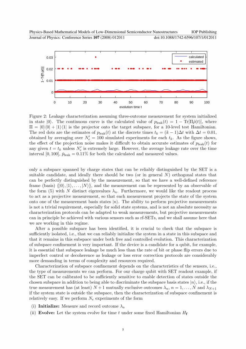
0 10 20 30 40 50 60 70 80 90 100
0
001
002
003
evolution time t
1minusT
r[Π ρ
(t)]
calculatedestimated
Figure 2 Leakage characterization assuming three-outcome measurement for system initializedin state |0〉 The continuous curve is the calculated value of pleak(t) = 1 minus Tr[Πρ(t)] whereΠ = |0〉〈0| + |1〉〈1| is the projector onto the target subspace for a 10-level test HamiltonianThe red dots are the estimates of pleak(t) at the discrete times tk = (k minus 1)∆t with ∆t = 001obtained by averaging over N prime
e = 100 simulated experiments for each tk As the figure showsthe effect of the projection noise makes it difficult to obtain accurate estimates of pleak(t) forany given t = tk unless N prime
e is extremely large However the average leakage rate over the timeinterval [0 100] pleak = 011 for both the calculated and measured values
only a subspace spanned by charge states that can be reliably distinguished by the SET is asuitable candidate and ideally there should be two (or in general N) orthogonal states thatcan be perfectly distinguished by the measurement so that we have a well-defined referenceframe (basis) |0〉 |1〉 |N〉 and the measurement can be represented by an observable ofthe form (5) with N distinct eigenvalues λn Furthermore we would like the readout processto act as a projective measurement so that each measurement projects the state of the systemonto one of the measurement basis states |n〉 The ability to perform projective measurementsis not a trivial requirement especially for solid state systems and is not an absolute necessity ascharacterization protocols can be adapted to weak measurements but projective measurementscan in principle be achieved with various sensors such as rf-SETs and we shall assume here thatwe are working in this regime
After a possible subspace has been identified it is crucial to check that the subspace issufficiently isolated ie that we can reliably initialize the system in a state in this subspace andthat it remains in this subspace under both free and controlled evolution This characterizationof subspace confinement is very important If the device is a candidate for a qubit for exampleit is essential that subspace leakage be much less than the rate of bit or phase flip errors due toimperfect control or decoherence as leakage or loss error correction protocols are considerablymore demanding in terms of complexity and resources required
Characterization of subspace confinement depends on the characteristics of the sensors iethe type of measurements we can perform For our charge qubit with SET readout example ifthe SET can be calibrated to be sufficiently sensitive to enable detection of states outside thechosen subspace in addition to being able to discriminate the subspace basis states |n〉 ie if thetrue measurement has (at least) N + 1 mutually exclusive outcomes λn n = 1 N and λN+1
if the system state is outside the subspace then the characterization of subspace confinement isrelatively easy If we perform Ne experiments of the form
(i) Initialize Measure and record outcome λa
(ii) Evolve Let the system evolve for time t under some fixed Hamiltonian Hf
Physics-Based Mathematical Models of Low-Dimensional Semiconductor Nanostructures IOP PublishingJournal of Physics Conference Series 107 (2008) 012011 doi1010881742-65961071012011
5
minus10 minus8 minus6 minus4 minus2 0 2 4 6 8 100
02
04
frequency ω
Re(
FT
[p0] )
02468 02468
05035
Ne=100 ∆ t=001
0 10 20 30 40 50 60 70 80 90 1000
05
1
t (arb units)
p 0(t)
Figure 3 p0(t) obtained by averaging over Ne = 100 simulated experiments with a 10-level testHamiltonian and corresponding Fourier spectrum From the 0th and 1st order peak heights weobtain h0 +2h1 = 09970 which yields upper and lower bounds for ε of asymp 00015 although thesebounds are statistically uncertain due to projection noise and discretization errors Nonethelessit can be verified that the actual subspace confinement for the chosen test Hamiltonian is 9994and thus the upper bound provides a reasonable estimate for the leakage
(iii) Measure Repeat measurement and record outcome λb
and denote by Nab the number of times the measurement results for the initial and finalmeasurements were λa and λb respectively then for Ne sufficiently large the leakage out of thesubspace is approximately equal to the fraction of experiments for which the first measurementwas λn with n le N and the second measurement was N + 1 ie
pleak asympsumN
n=1 NnN+1
Ne minussumN+1
n=1 NN+1n
(6)
Repeating the experiments for different evolution times t and averaging then gives an indicationof the rate of subspace leakage eg if we estimate pleak(tk) for tk = k∆t k = 0 K then
pleak =1
tmax
int tmax
0pleak(t) dt asymp 1
K + 1
Ksumk=0
pleak(tk) (7)
If the SET (or other measurement process) is not sufficiently sensitive to reliably distinguishat least N subspace basis states |n〉 as well as states outside the subspace then subspacecharacterization is more challenging For instance suppose we have a 2D subspace and asensor that can reliably detect only one state say |0〉 a common scenario for many systemswhere readout transitions are used that detect only a single state In this case the measurementoutcomes are λ0 or notλ0 If the measurement is projective and the dynamics confined to a 2Dsubspace we can identify notλ0 with outcome λ1 but this identification will lead to errors ifthe dynamics is not really confined to a 2D subspace However even in this case we can stillestimate the level of confinement to a 2D subspace under the evolution of a Hamiltonian Hf
Physics-Based Mathematical Models of Low-Dimensional Semiconductor Nanostructures IOP PublishingJournal of Physics Conference Series 107 (2008) 012011 doi1010881742-65961071012011
6
from observable coherent oscillations For example let
p0(t) = |〈0|eminusiHf t|0〉|2 (8)
be the probability of obtaining outcome λ0 when measuring the time-evolved state |Ψ(t)〉 =exp(minusitHf )|0〉 If the system is initialized in the state |0〉 and the dynamics of the system underHf is perfectly confined to a two-level subspace then conservation of probability implies that theheights h0 and h1 of the 0th and 1st order terms in the Fourier spectrum of p0(t) must satisfyh0 +2h1 = 1 We can use the deviation from this equality to bound the subspace leakage ε (11)
1minusradic
h0 + 2h1 le ε le 12(1minus
radic2(h0 + 2h1)minus 1) (9)
As the upper and lower bounds depend only on the 0th and 1st order Fourier peaks theycan usually be easily determined from experimental data although finite resolution due todiscretization and projection noise will reduce the accuracy of the estimates (11) Moreoverin this case 1minus ε only indicates the confinement of the system to some two-level subspace andwe must be careful as for different controls f the dynamics under Hf may be confined to differenttwo-level subspaces in which case the system cannot be considered a proper qubit For instancefor the 10-level test Hamiltonian
Htest =
13701 10000 00093 00055 00112 00068 00119 00084 00065 0008710000 15561 00109 00132 00067 00061 00081 00051 00105 0002900093 00109 16603 00034 00161 00100 00101 00123 00115 0005500055 00132 00034 19112 00136 00072 00093 00062 00133 0010100112 00067 00161 00136 34611 00022 00119 00078 00064 0012200068 00061 00100 00072 00022 43017 00074 00077 00029 0008000119 00081 00101 00093 00119 00074 68732 00133 00158 0015400084 00051 00123 00062 00078 00077 00133 73491 00071 0007300065 00105 00115 00133 00064 00029 00158 00071 81876 0010800087 00029 00055 00101 00122 00080 00154 00073 00108 89032
used for the simulated experiments in Figs 2 and 3 the first procedure measures the projectiononto the subspace S1 spanned by the measurement basis states |0〉 = (1 0 0 0 0 0 0 0 0 0 0)T
and |1〉 = (0 1 0 0 0 0 0 0 0 0 0)T while the second procedure measures the confinement ofthe dynamics to the best-fitting 2D subspace S2 which for the given Hamiltonian is spanned by
v1 = (1minus00001 00004 00034minus00012minus00002minus00005minus00004 00003minus00005)T
v2 = (0 1 00174 00238minus00131minus00051minus00032minus00020minus00022minus00013)T
and comparison of the results confirms that the average confinement 1minus pleak for the subspaceS1 as obtained by the first procedure is less (9989) than the confinement for subspace S2
(9994)
4 General characterization protocols for qubit systemsOnce a suitable subspace has been chosen we can proceed to the second stage of thecharacterization identification of the Hamiltonian and decoherence operators The simplesttype of system we can consider here is a qubit with Hilbert space dimension 2 In this case anynon-trivial projective measurement ie any measurement with two distinguishable outcomesλ0 and λ1 can be represented by an observable A = λ0|0〉〈0|+ λ1|1〉〈1| The eigenstates |0〉 and
Physics-Based Mathematical Models of Low-Dimensional Semiconductor Nanostructures IOP PublishingJournal of Physics Conference Series 107 (2008) 012011 doi1010881742-65961071012011
7
(a) (b)
Figure 4 Bloch sphere representation of dynamics (a) Arrangement of rotation axes dk withrespect to reference rotation axis dr (b) The evolution of the vector s(t) with s0 = (0 0 1)T
about the axis d and the projection of s(t) onto the z-axis
|1〉 of A define a basis for the Hilbert space and we can define the Pauli operators σ0 σx σy
and σz with respect to this basis
σ0 = |0〉〈0|+ |1〉〈1| σz = |0〉〈0| minus |1〉〈1| (10a)σx = |0〉〈1|+ |1〉〈0| σy = i(minus|0〉〈1|+ |1〉〈0|) (10b)
or in the usual matrix notation
σ0 =(
1 00 1
) σx =
(0 11 0
) σy =
(0 minusii 0
) σz =
(1 00 minus1
) (11)
Taking (without loss of generality) the measurement outcomes to be λ0 = 1 and λ1 = minus1 wehave A = σz in this basis Furthermore we can expand any Hamiltonian of the system as
H =12(d0σ0 + dxσx + dyσy + dzσz) (12a)
=d0
2σ0 +
ω
2(sin θ cos φ σx + sin θ sinφ σy + cos θ σz) (12b)
The d0 term can generally be ignored as the identity σ0 commutes with all other Pauli matricesand exp(minusitd0σ0) corresponds to multiplication by a global phase factor ie trivial dynamicsHence it suffices to determine the real vector d = (dx dy dz) or in polar form the angles(ω θ φ) to determine the Hamiltonian For a single Hamiltonian we can furthermore choosethe coordinate system such that φ = 0 However since H depends on control inputs f theparameters ω θ and φ also depend on the controls f and we usually need to determine Hf formany different f In this case we can choose a reference Hamiltonian eg Href with φ = 0 butwe must determine the relative angles φ with respect to the reference Hamiltonian for all othercontrol settings
41 Rotation frequency and declination of rotation axisTo relate the Hamiltonian parameters to observable dynamics it is instructive to visualize qubitstates and their evolution on the Bloch sphere If we define s = (sx sy sz)T with sk = Tr(ρσk)
Physics-Based Mathematical Models of Low-Dimensional Semiconductor Nanostructures IOP PublishingJournal of Physics Conference Series 107 (2008) 012011 doi1010881742-65961071012011
8
for k isin x y z then it is easy to check that there is a one-to-one correspondence betweendensity operators ρ and points s inside the closed unit Ball in IR3 Furthermore the evolutionof ρ(t) under the (constant) Hamiltonian (12) corresponds to a rotation of s(t) about the (unit)axis d = (sin θ cos φ sin θ sinφ cos θ)T with angular velocity ω as illustrated in Fig 4 Thefigure also shows that we can determine the angle θ and angular frequency d = ω from theprojection of s(t) under the rotation about the axis d onto the z-axis As the figure shows givenz(t) we can in principle extract ω and θ from the first minimum (t0 z0) of z(t) although inpractice it is usually preferable to use Fourier analysis or harmonic inversion techniques z(t)being the expectation value 〈A(t)〉 = Tr[σzρ(t)] of the observable A = σz in the state ρ(t) canbe obtained experimentally as follows (12)
(i) Initialize Measure and record outcome λa = plusmn1 rArr system in state λas0 = λa(0 0 1)T (ii) Evolve Let the system evolve for time t under the control settings f rArr system now in
state λas(t) = λa(x(t) y(t) z(t))T with
z(t) = cos2 θ + sin2 θ cos(ωt) (13)
(iii) Measure Repeat measurement and record outcome λb = plusmn1 rArr system now in state λbs0(iv) Repeat steps (i)ndash(iii) Ne times
Let Nab be the number of times the the initial measurement produced outcome λa and the finalmeasurement produced outcome λb Then there are four possible combinations of outcomesN00 N01 N10 and N11 which must add to the total number of experiments Ne The numberof experiments that started in the state |0〉 [or s0 = (0 0 1)T ] is N prime
e = N00 + N01 and thefraction of experiments for which the second measurement yields λ0 conditioned on the systemstarting in the state |0〉 is N00N
primee Thus the ensemble average of A = σz at time t assuming
we started in the state |0〉 is
λ0N00
N primee
+ λ1N01
N primee
=λ0N00 + λ1N01
N00 + N01 (14)
and for Ne rarr infin this relative frequency should approach the true expectation value of z(t)assuming z(0) = 1 Thus we can in principle determine z(t) to arbitrary accuracy by choosingNe large enough By repeating the experiments for different evolution times tk eg using astroboscopic mapping approach (see Fig 5) we can determine z(t) as a function of t from whichwe can extract ω = ωf and θ = θf as discussed For instance noting that z(t) = 2p0(t)minus1 Fig 3shows that the 1st order Fourier peak F (ω) of z(t) in this example is F (ω) asymp 2times02468 = 04935for ω asymp 2 and thus comparison with Eq (13) shows that sin2 θ = 2lt[F (ω)] or equivalentlyθ asymp 14566 These values are reasonably good estimates for the real values ω = 20086 andθ = minus14780 except for the sign of θ or the orientation of the rotation axis which we cannotdetermine from the given data as these rotations have identical projections onto the z-axisThis is reflected in Eq (13) by the fact that both coefficients cos2 θ and sin2 θ contain squaresIn principle we can determine the parameters ω and θ to arbitrary accuracy using this approachbased on regular sampling and Fourier analysis (13) although the total number of experimentscan become prohibitively large An alternative that merits further investigation is the use ofadaptive sampling techniques to reduce the total number of experiments necessary
42 Relative angles between rotation axesHaving determined the parameters ωf and θf for a particular control setting f and chosen asuitable reference Hamiltonian Href with φref = 0 to complete the characterization of Hf 6= Href we must determine the horizontal angle φf The reference Hamiltonian Href must not commute
Physics-Based Mathematical Models of Low-Dimensional Semiconductor Nanostructures IOP PublishingJournal of Physics Conference Series 107 (2008) 012011 doi1010881742-65961071012011
9
Init
Init
Init
Init
Meas
Meas
Meas
Meas
minus1
+1
z(t) = 〈σz〉
H(2∆t)
H(4∆t)
H(3∆t)
H(∆t)
Figure 5 Stroboscopic mapping of coherent oscillations with projective measurements Afterinitialization through measurement the system is allowed to evolve for fixed times under theinfluence of the controls before a second measurement is taken The experiments are repeatedto determine the expectation value of the observable at each time
with the measured observable A or equivalently the angle θref between the rotation axis dref
and the z-axis must be nonzero Ideally dref should be as close to orthogonal to the z-axis aspossible Assuming θref isin (π4 π2] and ωf and θf are known we can determine the angles φf
by performing the following experiments (12)
(i) Initialize Measure and record outcome λa = plusmn1 rArr system in state λas0 = λa(0 0 1)T (ii) Prepare Rotate around reference axis dref by angle α0 = arccos(1minusx
1+x) x = minus cos(2θref)rArr system in new state λas1 = λa(cos β sinβ 0)T with β = arctan(minus
radic2x) cos θref
(iii) Evolve Let the system evolve for time t under the control settings f rArr system in newstate λas(t) = λa(x(t) y(t) z(t))T with
z(t) = c[1minus cos(ωf t)] + d sin(ωf t) (15a)c = sin θf cos θf cos(φf minus β) (15b)d = sin θf sin(φf minus β) (15c)
(iv) Measure Repeat measurement and record outcome λb = plusmn1 rArr system in new state λbs0(v) Repeat steps (i)ndash(iv) Ne times
As before if Nab is the number of times the initial measurement produced outcome λa and thefinal measurement produced outcome λb then we have
z(t) asymp λ0N00 + λ1N01
N00 + N01
for sufficiently large Ne thus allowing us to determine z(t) experimentally Since θf ωf and β areknown from the θ ω characterization step Eq (15) allows us to determine φf via the coefficientsc and d which can be determined in principle either through curve fitting or by taking theFourier transform of z(t) and noting that c and d correspond to the real and imaginary part ofthe 0th and 1st order Fourier peaks
As a specific example assume we have two Hamiltonians H1 and H2 and we have alreadydetermined ω1 = 1 θ1 = π
4 and ω2 = 12 θ2 = π6 We choose H1 as reference Hamiltonian and
Physics-Based Mathematical Models of Low-Dimensional Semiconductor Nanostructures IOP PublishingJournal of Physics Conference Series 107 (2008) 012011 doi1010881742-65961071012011
10
0 10 20 30 40 50 60 70 80 90 100
minus05
0
05
1
evolution time t
z(t)
Ne=100 dt=001
minus15 minus1 minus05 0 05 1 15minus04
minus02
0
02
04
angular frequency ω
FT
(z) 0304466
Figure 6 Determination of relative horizontal angle between two Hamiltonians Measuredprojection z(t) of s1(t) onto the z-axis and corresponding Fourier spectrum Blueredbars indicate the cosinesine coefficients ie realimaginary parts of the Fourier transformrespectively
note that a rotation about H1 by α = π maps the state s0 = (0 0 1)T to s1 = (1 0 0)T Wethen let state s1 evolve for different length of time t under Hamiltonian H2 and determine theprojection z(t) This will produce a measured z-trace as shown in Fig 6 Eq (15) shows thatin theory the height of the real part of the 0th and 1st order Fourier peaks should be the sameexcept for the sign but the graph clearly shows that this is not the case for our noisy (simulated)experimental data In fact the 1st order peaks around plusmnωf are significantly broadened whilethe 0-peak is very narrow This suggests that we are likely to obtain the best estimate for φby setting c = FT[z](0) and φf = arccos[c(sin θf cos θf )] + β where β = 0 in our case Indeedthis yields an estimate of φf = 02518π which is very close to actual value π4 used in thesimulation Note that using the 1st order Fourier peaks gives far less accurate results due tothe significant broadening of the peaks This can be reduced using phase matching conditionsand other tricks (13) but in this case simply using only the 0-peak is sufficient to get a goodestimate
43 Functional dependence on control settingsIn some settings it is sufficient to characterize the Hamiltonians Hf for a discrete finite setof controls f (k) This would be the case for bang-bang-type control schemes that requireonly switching between a finite set of control Hamiltonians In other cases in particularwhen continuously varying fields are to be applied we would also like to know the functionaldependence of the Hamiltonian on the control fields eg whether we can assume a control-linearmodel as in (4) or if there are non-linear or crosstalk effects etc Although characterizing thecontrol dependence of the Hamiltonian is a non-trivial problem given sufficiently many Hf datapoints it is possible to test the quality of fit of a particular model using statistical means Forinstance suppose we have characterized the Hamiltonians Hf for f isin f (k) Let dk be thecorresponding vectors in IR3 as defined above and let f
(k)m be the mth component of the control
vector f (k) We can find the best-fitting linear model by finding vectors dm isin IR3 m = 0 M
Physics-Based Mathematical Models of Low-Dimensional Semiconductor Nanostructures IOP PublishingJournal of Physics Conference Series 107 (2008) 012011 doi1010881742-65961071012011
11
0 02 04 06 08 1 12 14 16 180
2
4
control input f (arb units)
x z
com
p o
f rot
axi
s
dx(f)
dz(f)
dz=1002minus0003f ∆=0013
dx=0006f+0996f2 ∆=0016
0 10 20 30 40 50 60 70 80 90 100
08
1
evolution time t
z(t)
Ne=100 dt=001 f=06
Figure 7 Determination of functional dependence of Hf on control input f The bottom graphshows the estimated values for d
(k)x and d
(k)z (circles and triangles respectively) as well as the
actual functional dependence in the model (solid lines) The top graph shows a typical z(t)trace obtained by averaging over Ne = 100 simulated experiments for each time tk = 001k Theeffects of finite sampling and projection noise are clearly visible for this trace Nonetheless thepredicted functional dependence of Hf on the control input f is in good agreement with theactual dependence in the model
where M is the number of independent control variables that minimize the norm of the residuals
∆ =radicsum
k rk22 where
rk = d0 +Msum
m=1
f (k)m dm minus dk (16)
The norm of the residuals ∆ then gives an indication of the quality of fit of a linear dependencemodel and allows us to compare the quality of fit for different models
As an example consider a Hamiltonian Hf depending on a one-dimensional control inputf = f To characterize the functional dependence of Hf on f we choose a finite set of controlsettings fk = 02(k minus 1) for k = 1 10 We characterize first the rotation frequencies ωk
and declination angles θk for each fk and then the relative angles φk as discussed above Fromthese we calculate the components d
(k)x d
(k)y and d
(k)z of the Hamiltonian according to Eq (12)
and plot them versus f as shown in Fig 7 Specifically in our case we find φk asymp 0 and hencedy equiv 0 dz appears to be constant and dx exhibits a quadratic dependence on the control f A least square fit of the data using a linear and quadratic fitting function respectively yieldsdz(f) = 1002 minus 0003 f and dx(t) = 0006f + 0996f2 which is in very good agreement withthe actual functional dependence in the model dz(f) = 1 and dx(f) = f2 despite the fact thatthe simulated data appears very noisy and the θ and ω estimates did not employ tuning such asphase matching to further improve the accuracy
44 Characterization in the presence of decoherenceThe protocols for Hamiltonian identification above are sufficient if dissipative effects are small onthe timescales for coherent control ie if the system and environment coupling is much weaker
Physics-Based Mathematical Models of Low-Dimensional Semiconductor Nanostructures IOP PublishingJournal of Physics Conference Series 107 (2008) 012011 doi1010881742-65961071012011
12
than the system-control interaction If the coupling between the system and its environment isstronger then dissipative effects must be directly incorporated into the characterization protocols
Assuming Markovian decoherence of the form (2) it is easy to show that for N = 2 wehave Ak = U σkU
dagger where σk are the elementary relaxation operators σminus σ+ 12 σz defined
in terms of the Pauli matrices σplusmn = 12(σx ∓ iσy) and U is some unitary operator in SU(2)
that defines a preferred decoherence basis The operator σz is usually associated with puredecoherence (pure dephasing) while the raising and lowering operators σplusmn are associated withpopulation relaxation from |1〉 to |0〉 and vice versa Very often it is furthermore assumed thatU = I is the identity ie that the preferred basis for relaxation is the same as the measurementbasis Although this need not be the case it is often a good approximation The main effectof relaxation processes is to dampen the observed coherent oscillations z(t) that result from theHamiltonian dynamics and try to force the system lsquoasymptoticallyrsquo into a lsquosteadyrsquo state Thiseffect manifests itself in Lorentzian broadening of the peaks in the oscillation spectrum whichcan be used for characterization purposes
For example Fig 8 shows significantly damped oscillations as a result of relaxation The factthat the oscillations decay to zinfin = 0 suggests either pure dephasing or a symmetric relaxationprocess with Γ+ = Γminus ie equal probability of relaxation from state |0〉 to |1〉 and vice versaor a combination of both Since symmetric relaxation and pure dephasing have very similarsignatures it can be difficult to distinguish these processes from the oscillation trace aloneHowever if there exists a control f such that Hf prop σz which corresponds to a rotation aboutthe z (or measurement) axis then we can in principle distinguish the two processes by initializingthe system repeatedly in either state |0〉 or |1〉 and letting the system evolve under Hf for variousperiods of time before measuring again If the decoherence process is pure dephasing then thesystem will remain in the initial state while we expect to observe random jumps (with equalprobability) for symmetric relaxation Assuming this preliminary characterization step suggeststhat the damping in the figure is due to pure dephasing we can then extract information aboutthe rotation frequency ω0 and dephasing rate Γ by fitting a Lorentzian envelope function
Lω0Γ(ω) =Γ
(ω minus ω0)2 + Γ2(17)
to the first-order peak in the Fourier spectrum as shown in the figure In our example usinga simple least-squares minimization yields estimated values for both ω0 and Γ that are close tothe actual values used in the simulated experiment This approach can be generalized for morecomplicated relaxation processes (14) Alternatively if we can characterize the Hamiltoniandynamics sufficiently to be able to initialize the system in non-measurement basis states andsimulate readout in different bases then generalized Lindblad operators can be estimated usingrepeated process tomography (15)
5 Discussion of generalizations and conclusionsWe have described some basic tools and techniques for characterizing the extent to whichthe dynamics of a certain system is confined to a low-dimensional subspace of a potentiallylarge Hilbert space as well as for identifying both Hamiltonian and decoherence parametersexperimentally with emphasis on protocols that are realistic even in the presence of limiteddirect readout and control capabilities
Although the explicit schemes presented focused on qubit-like systems the same basic ideascan be applied to higher-dimensional systems However the number of Hamiltonian anddecoherence parameters to be determined for higher-dimensional system makes finding explicitprotocols for complete characterization quite challenging The qubit characterization protocolsshow that identifying the relative angles between several control Hamiltonians requires a two-stage process and more complicated two-step experiments (initialization in non-measurement
Physics-Based Mathematical Models of Low-Dimensional Semiconductor Nanostructures IOP PublishingJournal of Physics Conference Series 107 (2008) 012011 doi1010881742-65961071012011
13
0 10 20 30 40 50 60 70 80 90 1000
05
1
evolution time t
z(t)
ω0=1414
Γ=01
minus15 minus1 minus05 0 05 1 150
002
004
006
angular frequency ω
Re[
FT
(z)]
ω
0est=1406
Γest
=009703Re FT[z]
Lorentzian fit
Figure 8 Characterization in the presence of decoherence The observed damped oscillationsdue to pure dephasing (top) result in Lorentzian broadening of the Fourier peaks which can beexploited to obtain (good) estimates for the rotation frequency ω0 and decoherence rate Γ
basis state followed by controlled evolution) than identifying the rotation frequency anddeclination angle for a single Hamiltonian As the dimension of the system increases moreparameters are necessary to fully characterize the Hamiltonians leading to more complex multi-stage characterization protocols
Another problem is that the number of experiments required to implement such schemesmay become prohibitively large for parameter estimation based on spectroscopic analysis Oneof the most promising strategies to avoid this problem is the development of efficient adaptivecharacterization schemesmdashas opposed to protocols based on regular samplingmdash to minimize thenumber of measurements experiments required For systems composed of separate smaller unitssuch as multi-qubit systems boot-strapping approaches to characterization may also provide afruitful alternative For example assuming we have separately characterized individual qubitsusing qubit identification protocols and therefore have full local control we can reduce theproblem of two-qubit identification in principle to identifying the interaction Hamiltonian Fortwo-qubit systems with local control and a fully non-local interaction Hamiltonian this can beachieved using entanglement mapping or concurrence spectroscopy (16 17)
AcknowledgmentsSGS acknowledges funding from an EPSRC Advanced Research Fellowship and support fromHitachi and the EPSRC QIP IRC DKLO is supported by a SUPA fellowship SJD acknowledgessupport from MEXT
References[1] Nielsen M A and Chuang I L 2000 Quantum Computation and Quantum Information
(Cambridge UK Cambridge University Press)[2] Gorman J Hasko D G and Williams D A 2005 Phys Rev Lett 95 090502[3] Lindblad G 1976 Comm Math Phys 48 119ndash130[4] Gorini V Kossakowski A and Sudarshan E C G 1976 J Math Phys 17 821ndash825
Physics-Based Mathematical Models of Low-Dimensional Semiconductor Nanostructures IOP PublishingJournal of Physics Conference Series 107 (2008) 012011 doi1010881742-65961071012011
14
[5] Devoret M H and Schoelkopf R J 2000 Nature 406 1039[6] Chuang I L and Nielson M A 1997 J Mod Opt 44 2455[7] Poyatos J F Cirac J I and Zoller P 1997 Phys Rev Lett 78 0390[8] Leung D W 2003 J Math Phys 44 0528[9] Thew R T Nemoto K White A G and Munro W J 2002 Phys Rev A 66 012303
[10] Kosut R Walmsley I A and Rabitz H 2004 Optimal experiment design for quantum stateand progress tomography and Hamiltonian parameter estimation quant-ph0411093
[11] Devitt S J Schirmer S G Oi D K L Cole J H and Hollenberg L C L 2007 New J Physics7 384
[12] Schirmer S G Kolli A and Oi D K L 2004 Phys Rev A 69 050603(R)[13] Cole J H Schirmer S G Greentree A D Wellard C J Oi D K L and Hollenberg L C L 2005
Phys Rev A 71 062312[14] Cole J H Greentree A D Oi D K L Schirmer S G Wellard C J and Hollenberg L C L 2006
Phys Rev A 73 062333[15] Boulant N Havel T F Pravia M A and Cory D G 2003 Phys Rev A 67 042322[16] Devitt S J Cole J H and Hollenberg L C L 2006 Phys Rev A 73 052317[17] Cole J Devitt S and Hollenberg L 2006 J Phys A 39 14649ndash14658
Physics-Based Mathematical Models of Low-Dimensional Semiconductor Nanostructures IOP PublishingJournal of Physics Conference Series 107 (2008) 012011 doi1010881742-65961071012011
15
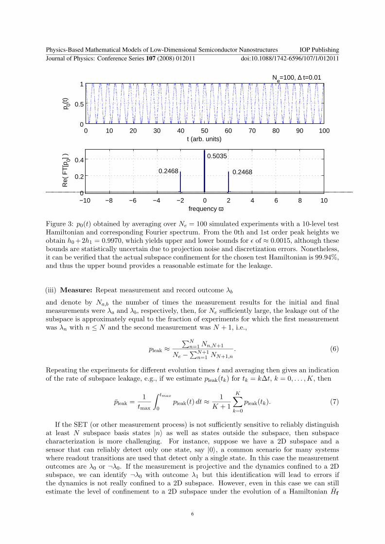
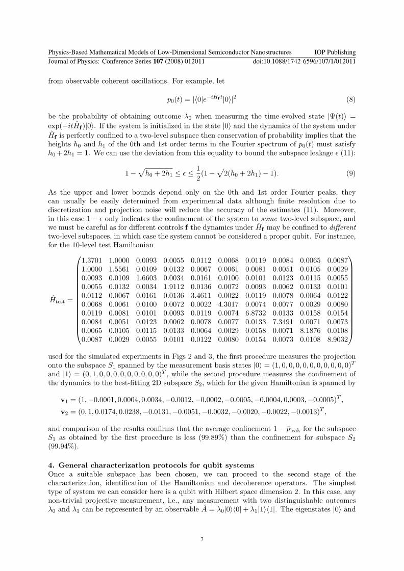
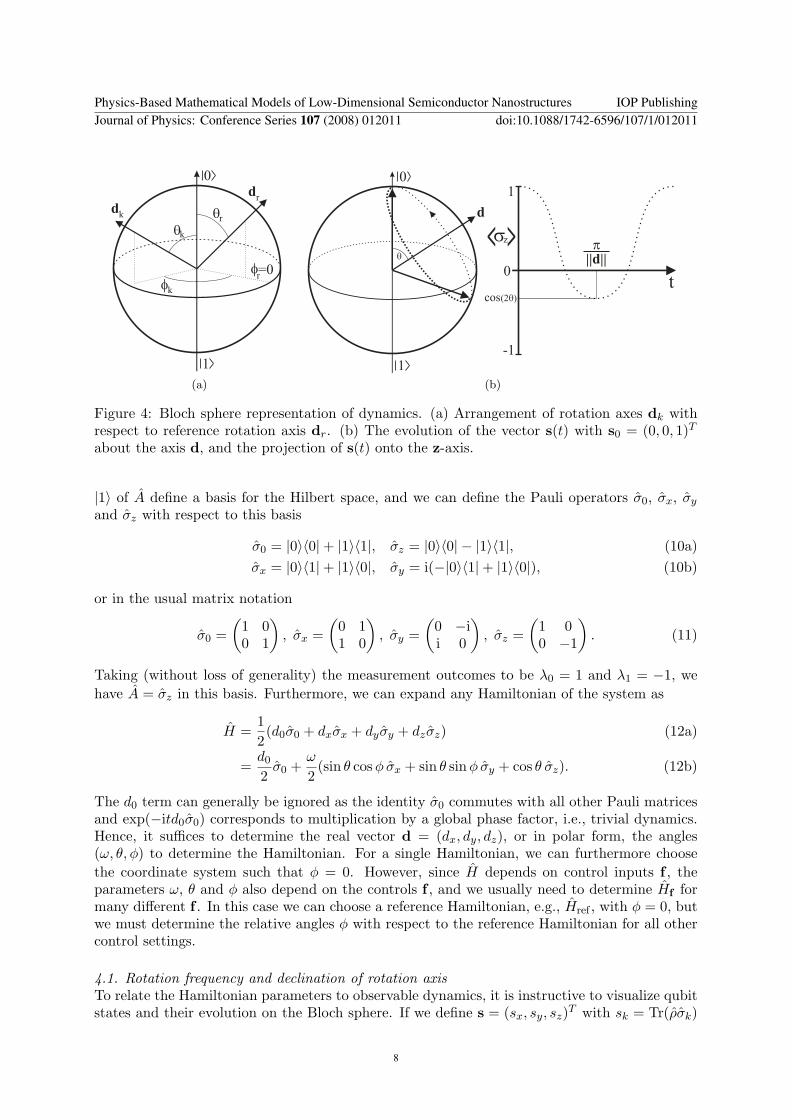
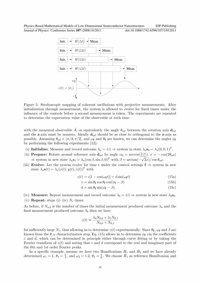
Init
Init
Init
Init
Meas
Meas
Meas
Meas
minus1
+1
z(t) = 〈σz〉
H(2∆t)
H(4∆t)
H(3∆t)
H(∆t)
Figure 5 Stroboscopic mapping of coherent oscillations with projective measurements Afterinitialization through measurement the system is allowed to evolve for fixed times under theinfluence of the controls before a second measurement is taken The experiments are repeatedto determine the expectation value of the observable at each time
with the measured observable A or equivalently the angle θref between the rotation axis dref
and the z-axis must be nonzero Ideally dref should be as close to orthogonal to the z-axis aspossible Assuming θref isin (π4 π2] and ωf and θf are known we can determine the angles φf
by performing the following experiments (12)
(i) Initialize Measure and record outcome λa = plusmn1 rArr system in state λas0 = λa(0 0 1)T (ii) Prepare Rotate around reference axis dref by angle α0 = arccos(1minusx
1+x) x = minus cos(2θref)rArr system in new state λas1 = λa(cos β sinβ 0)T with β = arctan(minus
radic2x) cos θref
(iii) Evolve Let the system evolve for time t under the control settings f rArr system in newstate λas(t) = λa(x(t) y(t) z(t))T with
z(t) = c[1minus cos(ωf t)] + d sin(ωf t) (15a)c = sin θf cos θf cos(φf minus β) (15b)d = sin θf sin(φf minus β) (15c)
(iv) Measure Repeat measurement and record outcome λb = plusmn1 rArr system in new state λbs0(v) Repeat steps (i)ndash(iv) Ne times
As before if Nab is the number of times the initial measurement produced outcome λa and thefinal measurement produced outcome λb then we have
z(t) asymp λ0N00 + λ1N01
N00 + N01
for sufficiently large Ne thus allowing us to determine z(t) experimentally Since θf ωf and β areknown from the θ ω characterization step Eq (15) allows us to determine φf via the coefficientsc and d which can be determined in principle either through curve fitting or by taking theFourier transform of z(t) and noting that c and d correspond to the real and imaginary part ofthe 0th and 1st order Fourier peaks
As a specific example assume we have two Hamiltonians H1 and H2 and we have alreadydetermined ω1 = 1 θ1 = π
4 and ω2 = 12 θ2 = π6 We choose H1 as reference Hamiltonian and
Physics-Based Mathematical Models of Low-Dimensional Semiconductor Nanostructures IOP PublishingJournal of Physics Conference Series 107 (2008) 012011 doi1010881742-65961071012011
10
0 10 20 30 40 50 60 70 80 90 100
minus05
0
05
1
evolution time t
z(t)
Ne=100 dt=001
minus15 minus1 minus05 0 05 1 15minus04
minus02
0
02
04
angular frequency ω
FT
(z) 0304466
Figure 6 Determination of relative horizontal angle between two Hamiltonians Measuredprojection z(t) of s1(t) onto the z-axis and corresponding Fourier spectrum Blueredbars indicate the cosinesine coefficients ie realimaginary parts of the Fourier transformrespectively
note that a rotation about H1 by α = π maps the state s0 = (0 0 1)T to s1 = (1 0 0)T Wethen let state s1 evolve for different length of time t under Hamiltonian H2 and determine theprojection z(t) This will produce a measured z-trace as shown in Fig 6 Eq (15) shows thatin theory the height of the real part of the 0th and 1st order Fourier peaks should be the sameexcept for the sign but the graph clearly shows that this is not the case for our noisy (simulated)experimental data In fact the 1st order peaks around plusmnωf are significantly broadened whilethe 0-peak is very narrow This suggests that we are likely to obtain the best estimate for φby setting c = FT[z](0) and φf = arccos[c(sin θf cos θf )] + β where β = 0 in our case Indeedthis yields an estimate of φf = 02518π which is very close to actual value π4 used in thesimulation Note that using the 1st order Fourier peaks gives far less accurate results due tothe significant broadening of the peaks This can be reduced using phase matching conditionsand other tricks (13) but in this case simply using only the 0-peak is sufficient to get a goodestimate
43 Functional dependence on control settingsIn some settings it is sufficient to characterize the Hamiltonians Hf for a discrete finite setof controls f (k) This would be the case for bang-bang-type control schemes that requireonly switching between a finite set of control Hamiltonians In other cases in particularwhen continuously varying fields are to be applied we would also like to know the functionaldependence of the Hamiltonian on the control fields eg whether we can assume a control-linearmodel as in (4) or if there are non-linear or crosstalk effects etc Although characterizing thecontrol dependence of the Hamiltonian is a non-trivial problem given sufficiently many Hf datapoints it is possible to test the quality of fit of a particular model using statistical means Forinstance suppose we have characterized the Hamiltonians Hf for f isin f (k) Let dk be thecorresponding vectors in IR3 as defined above and let f
(k)m be the mth component of the control
vector f (k) We can find the best-fitting linear model by finding vectors dm isin IR3 m = 0 M
Physics-Based Mathematical Models of Low-Dimensional Semiconductor Nanostructures IOP PublishingJournal of Physics Conference Series 107 (2008) 012011 doi1010881742-65961071012011
11
0 02 04 06 08 1 12 14 16 180
2
4
control input f (arb units)
x z
com
p o
f rot
axi
s
dx(f)
dz(f)
dz=1002minus0003f ∆=0013
dx=0006f+0996f2 ∆=0016
0 10 20 30 40 50 60 70 80 90 100
08
1
evolution time t
z(t)
Ne=100 dt=001 f=06
Figure 7 Determination of functional dependence of Hf on control input f The bottom graphshows the estimated values for d
(k)x and d
(k)z (circles and triangles respectively) as well as the
actual functional dependence in the model (solid lines) The top graph shows a typical z(t)trace obtained by averaging over Ne = 100 simulated experiments for each time tk = 001k Theeffects of finite sampling and projection noise are clearly visible for this trace Nonetheless thepredicted functional dependence of Hf on the control input f is in good agreement with theactual dependence in the model
where M is the number of independent control variables that minimize the norm of the residuals
∆ =radicsum
k rk22 where
rk = d0 +Msum
m=1
f (k)m dm minus dk (16)
The norm of the residuals ∆ then gives an indication of the quality of fit of a linear dependencemodel and allows us to compare the quality of fit for different models
As an example consider a Hamiltonian Hf depending on a one-dimensional control inputf = f To characterize the functional dependence of Hf on f we choose a finite set of controlsettings fk = 02(k minus 1) for k = 1 10 We characterize first the rotation frequencies ωk
and declination angles θk for each fk and then the relative angles φk as discussed above Fromthese we calculate the components d
(k)x d
(k)y and d
(k)z of the Hamiltonian according to Eq (12)
and plot them versus f as shown in Fig 7 Specifically in our case we find φk asymp 0 and hencedy equiv 0 dz appears to be constant and dx exhibits a quadratic dependence on the control f A least square fit of the data using a linear and quadratic fitting function respectively yieldsdz(f) = 1002 minus 0003 f and dx(t) = 0006f + 0996f2 which is in very good agreement withthe actual functional dependence in the model dz(f) = 1 and dx(f) = f2 despite the fact thatthe simulated data appears very noisy and the θ and ω estimates did not employ tuning such asphase matching to further improve the accuracy
44 Characterization in the presence of decoherenceThe protocols for Hamiltonian identification above are sufficient if dissipative effects are small onthe timescales for coherent control ie if the system and environment coupling is much weaker
Physics-Based Mathematical Models of Low-Dimensional Semiconductor Nanostructures IOP PublishingJournal of Physics Conference Series 107 (2008) 012011 doi1010881742-65961071012011
12
than the system-control interaction If the coupling between the system and its environment isstronger then dissipative effects must be directly incorporated into the characterization protocols
Assuming Markovian decoherence of the form (2) it is easy to show that for N = 2 wehave Ak = U σkU
dagger where σk are the elementary relaxation operators σminus σ+ 12 σz defined
in terms of the Pauli matrices σplusmn = 12(σx ∓ iσy) and U is some unitary operator in SU(2)
that defines a preferred decoherence basis The operator σz is usually associated with puredecoherence (pure dephasing) while the raising and lowering operators σplusmn are associated withpopulation relaxation from |1〉 to |0〉 and vice versa Very often it is furthermore assumed thatU = I is the identity ie that the preferred basis for relaxation is the same as the measurementbasis Although this need not be the case it is often a good approximation The main effectof relaxation processes is to dampen the observed coherent oscillations z(t) that result from theHamiltonian dynamics and try to force the system lsquoasymptoticallyrsquo into a lsquosteadyrsquo state Thiseffect manifests itself in Lorentzian broadening of the peaks in the oscillation spectrum whichcan be used for characterization purposes
For example Fig 8 shows significantly damped oscillations as a result of relaxation The factthat the oscillations decay to zinfin = 0 suggests either pure dephasing or a symmetric relaxationprocess with Γ+ = Γminus ie equal probability of relaxation from state |0〉 to |1〉 and vice versaor a combination of both Since symmetric relaxation and pure dephasing have very similarsignatures it can be difficult to distinguish these processes from the oscillation trace aloneHowever if there exists a control f such that Hf prop σz which corresponds to a rotation aboutthe z (or measurement) axis then we can in principle distinguish the two processes by initializingthe system repeatedly in either state |0〉 or |1〉 and letting the system evolve under Hf for variousperiods of time before measuring again If the decoherence process is pure dephasing then thesystem will remain in the initial state while we expect to observe random jumps (with equalprobability) for symmetric relaxation Assuming this preliminary characterization step suggeststhat the damping in the figure is due to pure dephasing we can then extract information aboutthe rotation frequency ω0 and dephasing rate Γ by fitting a Lorentzian envelope function
Lω0Γ(ω) =Γ
(ω minus ω0)2 + Γ2(17)
to the first-order peak in the Fourier spectrum as shown in the figure In our example usinga simple least-squares minimization yields estimated values for both ω0 and Γ that are close tothe actual values used in the simulated experiment This approach can be generalized for morecomplicated relaxation processes (14) Alternatively if we can characterize the Hamiltoniandynamics sufficiently to be able to initialize the system in non-measurement basis states andsimulate readout in different bases then generalized Lindblad operators can be estimated usingrepeated process tomography (15)
5 Discussion of generalizations and conclusionsWe have described some basic tools and techniques for characterizing the extent to whichthe dynamics of a certain system is confined to a low-dimensional subspace of a potentiallylarge Hilbert space as well as for identifying both Hamiltonian and decoherence parametersexperimentally with emphasis on protocols that are realistic even in the presence of limiteddirect readout and control capabilities
Although the explicit schemes presented focused on qubit-like systems the same basic ideascan be applied to higher-dimensional systems However the number of Hamiltonian anddecoherence parameters to be determined for higher-dimensional system makes finding explicitprotocols for complete characterization quite challenging The qubit characterization protocolsshow that identifying the relative angles between several control Hamiltonians requires a two-stage process and more complicated two-step experiments (initialization in non-measurement
Physics-Based Mathematical Models of Low-Dimensional Semiconductor Nanostructures IOP PublishingJournal of Physics Conference Series 107 (2008) 012011 doi1010881742-65961071012011
13
0 10 20 30 40 50 60 70 80 90 1000
05
1
evolution time t
z(t)
ω0=1414
Γ=01
minus15 minus1 minus05 0 05 1 150
002
004
006
angular frequency ω
Re[
FT
(z)]
ω
0est=1406
Γest
=009703Re FT[z]
Lorentzian fit
Figure 8 Characterization in the presence of decoherence The observed damped oscillationsdue to pure dephasing (top) result in Lorentzian broadening of the Fourier peaks which can beexploited to obtain (good) estimates for the rotation frequency ω0 and decoherence rate Γ
basis state followed by controlled evolution) than identifying the rotation frequency anddeclination angle for a single Hamiltonian As the dimension of the system increases moreparameters are necessary to fully characterize the Hamiltonians leading to more complex multi-stage characterization protocols
Another problem is that the number of experiments required to implement such schemesmay become prohibitively large for parameter estimation based on spectroscopic analysis Oneof the most promising strategies to avoid this problem is the development of efficient adaptivecharacterization schemesmdashas opposed to protocols based on regular samplingmdash to minimize thenumber of measurements experiments required For systems composed of separate smaller unitssuch as multi-qubit systems boot-strapping approaches to characterization may also provide afruitful alternative For example assuming we have separately characterized individual qubitsusing qubit identification protocols and therefore have full local control we can reduce theproblem of two-qubit identification in principle to identifying the interaction Hamiltonian Fortwo-qubit systems with local control and a fully non-local interaction Hamiltonian this can beachieved using entanglement mapping or concurrence spectroscopy (16 17)
AcknowledgmentsSGS acknowledges funding from an EPSRC Advanced Research Fellowship and support fromHitachi and the EPSRC QIP IRC DKLO is supported by a SUPA fellowship SJD acknowledgessupport from MEXT
References[1] Nielsen M A and Chuang I L 2000 Quantum Computation and Quantum Information
(Cambridge UK Cambridge University Press)[2] Gorman J Hasko D G and Williams D A 2005 Phys Rev Lett 95 090502[3] Lindblad G 1976 Comm Math Phys 48 119ndash130[4] Gorini V Kossakowski A and Sudarshan E C G 1976 J Math Phys 17 821ndash825
Physics-Based Mathematical Models of Low-Dimensional Semiconductor Nanostructures IOP PublishingJournal of Physics Conference Series 107 (2008) 012011 doi1010881742-65961071012011
14
[5] Devoret M H and Schoelkopf R J 2000 Nature 406 1039[6] Chuang I L and Nielson M A 1997 J Mod Opt 44 2455[7] Poyatos J F Cirac J I and Zoller P 1997 Phys Rev Lett 78 0390[8] Leung D W 2003 J Math Phys 44 0528[9] Thew R T Nemoto K White A G and Munro W J 2002 Phys Rev A 66 012303
[10] Kosut R Walmsley I A and Rabitz H 2004 Optimal experiment design for quantum stateand progress tomography and Hamiltonian parameter estimation quant-ph0411093
[11] Devitt S J Schirmer S G Oi D K L Cole J H and Hollenberg L C L 2007 New J Physics7 384
[12] Schirmer S G Kolli A and Oi D K L 2004 Phys Rev A 69 050603(R)[13] Cole J H Schirmer S G Greentree A D Wellard C J Oi D K L and Hollenberg L C L 2005
Phys Rev A 71 062312[14] Cole J H Greentree A D Oi D K L Schirmer S G Wellard C J and Hollenberg L C L 2006
Phys Rev A 73 062333[15] Boulant N Havel T F Pravia M A and Cory D G 2003 Phys Rev A 67 042322[16] Devitt S J Cole J H and Hollenberg L C L 2006 Phys Rev A 73 052317[17] Cole J Devitt S and Hollenberg L 2006 J Phys A 39 14649ndash14658
Physics-Based Mathematical Models of Low-Dimensional Semiconductor Nanostructures IOP PublishingJournal of Physics Conference Series 107 (2008) 012011 doi1010881742-65961071012011
15
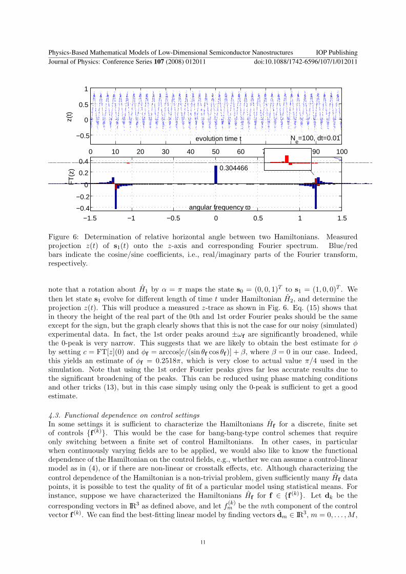
0 10 20 30 40 50 60 70 80 90 100
minus05
0
05
1
evolution time t
z(t)
Ne=100 dt=001
minus15 minus1 minus05 0 05 1 15minus04
minus02
0
02
04
angular frequency ω
FT
(z) 0304466
Figure 6 Determination of relative horizontal angle between two Hamiltonians Measuredprojection z(t) of s1(t) onto the z-axis and corresponding Fourier spectrum Blueredbars indicate the cosinesine coefficients ie realimaginary parts of the Fourier transformrespectively
note that a rotation about H1 by α = π maps the state s0 = (0 0 1)T to s1 = (1 0 0)T Wethen let state s1 evolve for different length of time t under Hamiltonian H2 and determine theprojection z(t) This will produce a measured z-trace as shown in Fig 6 Eq (15) shows thatin theory the height of the real part of the 0th and 1st order Fourier peaks should be the sameexcept for the sign but the graph clearly shows that this is not the case for our noisy (simulated)experimental data In fact the 1st order peaks around plusmnωf are significantly broadened whilethe 0-peak is very narrow This suggests that we are likely to obtain the best estimate for φby setting c = FT[z](0) and φf = arccos[c(sin θf cos θf )] + β where β = 0 in our case Indeedthis yields an estimate of φf = 02518π which is very close to actual value π4 used in thesimulation Note that using the 1st order Fourier peaks gives far less accurate results due tothe significant broadening of the peaks This can be reduced using phase matching conditionsand other tricks (13) but in this case simply using only the 0-peak is sufficient to get a goodestimate
43 Functional dependence on control settingsIn some settings it is sufficient to characterize the Hamiltonians Hf for a discrete finite setof controls f (k) This would be the case for bang-bang-type control schemes that requireonly switching between a finite set of control Hamiltonians In other cases in particularwhen continuously varying fields are to be applied we would also like to know the functionaldependence of the Hamiltonian on the control fields eg whether we can assume a control-linearmodel as in (4) or if there are non-linear or crosstalk effects etc Although characterizing thecontrol dependence of the Hamiltonian is a non-trivial problem given sufficiently many Hf datapoints it is possible to test the quality of fit of a particular model using statistical means Forinstance suppose we have characterized the Hamiltonians Hf for f isin f (k) Let dk be thecorresponding vectors in IR3 as defined above and let f
(k)m be the mth component of the control
vector f (k) We can find the best-fitting linear model by finding vectors dm isin IR3 m = 0 M
Physics-Based Mathematical Models of Low-Dimensional Semiconductor Nanostructures IOP PublishingJournal of Physics Conference Series 107 (2008) 012011 doi1010881742-65961071012011
11
0 02 04 06 08 1 12 14 16 180
2
4
control input f (arb units)
x z
com
p o
f rot
axi
s
dx(f)
dz(f)
dz=1002minus0003f ∆=0013
dx=0006f+0996f2 ∆=0016
0 10 20 30 40 50 60 70 80 90 100
08
1
evolution time t
z(t)
Ne=100 dt=001 f=06
Figure 7 Determination of functional dependence of Hf on control input f The bottom graphshows the estimated values for d
(k)x and d
(k)z (circles and triangles respectively) as well as the
actual functional dependence in the model (solid lines) The top graph shows a typical z(t)trace obtained by averaging over Ne = 100 simulated experiments for each time tk = 001k Theeffects of finite sampling and projection noise are clearly visible for this trace Nonetheless thepredicted functional dependence of Hf on the control input f is in good agreement with theactual dependence in the model
where M is the number of independent control variables that minimize the norm of the residuals
∆ =radicsum
k rk22 where
rk = d0 +Msum
m=1
f (k)m dm minus dk (16)
The norm of the residuals ∆ then gives an indication of the quality of fit of a linear dependencemodel and allows us to compare the quality of fit for different models
As an example consider a Hamiltonian Hf depending on a one-dimensional control inputf = f To characterize the functional dependence of Hf on f we choose a finite set of controlsettings fk = 02(k minus 1) for k = 1 10 We characterize first the rotation frequencies ωk
and declination angles θk for each fk and then the relative angles φk as discussed above Fromthese we calculate the components d
(k)x d
(k)y and d
(k)z of the Hamiltonian according to Eq (12)
and plot them versus f as shown in Fig 7 Specifically in our case we find φk asymp 0 and hencedy equiv 0 dz appears to be constant and dx exhibits a quadratic dependence on the control f A least square fit of the data using a linear and quadratic fitting function respectively yieldsdz(f) = 1002 minus 0003 f and dx(t) = 0006f + 0996f2 which is in very good agreement withthe actual functional dependence in the model dz(f) = 1 and dx(f) = f2 despite the fact thatthe simulated data appears very noisy and the θ and ω estimates did not employ tuning such asphase matching to further improve the accuracy
44 Characterization in the presence of decoherenceThe protocols for Hamiltonian identification above are sufficient if dissipative effects are small onthe timescales for coherent control ie if the system and environment coupling is much weaker
Physics-Based Mathematical Models of Low-Dimensional Semiconductor Nanostructures IOP PublishingJournal of Physics Conference Series 107 (2008) 012011 doi1010881742-65961071012011
12
than the system-control interaction If the coupling between the system and its environment isstronger then dissipative effects must be directly incorporated into the characterization protocols
Assuming Markovian decoherence of the form (2) it is easy to show that for N = 2 wehave Ak = U σkU
dagger where σk are the elementary relaxation operators σminus σ+ 12 σz defined
in terms of the Pauli matrices σplusmn = 12(σx ∓ iσy) and U is some unitary operator in SU(2)
that defines a preferred decoherence basis The operator σz is usually associated with puredecoherence (pure dephasing) while the raising and lowering operators σplusmn are associated withpopulation relaxation from |1〉 to |0〉 and vice versa Very often it is furthermore assumed thatU = I is the identity ie that the preferred basis for relaxation is the same as the measurementbasis Although this need not be the case it is often a good approximation The main effectof relaxation processes is to dampen the observed coherent oscillations z(t) that result from theHamiltonian dynamics and try to force the system lsquoasymptoticallyrsquo into a lsquosteadyrsquo state Thiseffect manifests itself in Lorentzian broadening of the peaks in the oscillation spectrum whichcan be used for characterization purposes
For example Fig 8 shows significantly damped oscillations as a result of relaxation The factthat the oscillations decay to zinfin = 0 suggests either pure dephasing or a symmetric relaxationprocess with Γ+ = Γminus ie equal probability of relaxation from state |0〉 to |1〉 and vice versaor a combination of both Since symmetric relaxation and pure dephasing have very similarsignatures it can be difficult to distinguish these processes from the oscillation trace aloneHowever if there exists a control f such that Hf prop σz which corresponds to a rotation aboutthe z (or measurement) axis then we can in principle distinguish the two processes by initializingthe system repeatedly in either state |0〉 or |1〉 and letting the system evolve under Hf for variousperiods of time before measuring again If the decoherence process is pure dephasing then thesystem will remain in the initial state while we expect to observe random jumps (with equalprobability) for symmetric relaxation Assuming this preliminary characterization step suggeststhat the damping in the figure is due to pure dephasing we can then extract information aboutthe rotation frequency ω0 and dephasing rate Γ by fitting a Lorentzian envelope function
Lω0Γ(ω) =Γ
(ω minus ω0)2 + Γ2(17)
to the first-order peak in the Fourier spectrum as shown in the figure In our example usinga simple least-squares minimization yields estimated values for both ω0 and Γ that are close tothe actual values used in the simulated experiment This approach can be generalized for morecomplicated relaxation processes (14) Alternatively if we can characterize the Hamiltoniandynamics sufficiently to be able to initialize the system in non-measurement basis states andsimulate readout in different bases then generalized Lindblad operators can be estimated usingrepeated process tomography (15)
5 Discussion of generalizations and conclusionsWe have described some basic tools and techniques for characterizing the extent to whichthe dynamics of a certain system is confined to a low-dimensional subspace of a potentiallylarge Hilbert space as well as for identifying both Hamiltonian and decoherence parametersexperimentally with emphasis on protocols that are realistic even in the presence of limiteddirect readout and control capabilities
Although the explicit schemes presented focused on qubit-like systems the same basic ideascan be applied to higher-dimensional systems However the number of Hamiltonian anddecoherence parameters to be determined for higher-dimensional system makes finding explicitprotocols for complete characterization quite challenging The qubit characterization protocolsshow that identifying the relative angles between several control Hamiltonians requires a two-stage process and more complicated two-step experiments (initialization in non-measurement
Physics-Based Mathematical Models of Low-Dimensional Semiconductor Nanostructures IOP PublishingJournal of Physics Conference Series 107 (2008) 012011 doi1010881742-65961071012011
13
0 10 20 30 40 50 60 70 80 90 1000
05
1
evolution time t
z(t)
ω0=1414
Γ=01
minus15 minus1 minus05 0 05 1 150
002
004
006
angular frequency ω
Re[
FT
(z)]
ω
0est=1406
Γest
=009703Re FT[z]
Lorentzian fit
Figure 8 Characterization in the presence of decoherence The observed damped oscillationsdue to pure dephasing (top) result in Lorentzian broadening of the Fourier peaks which can beexploited to obtain (good) estimates for the rotation frequency ω0 and decoherence rate Γ
basis state followed by controlled evolution) than identifying the rotation frequency anddeclination angle for a single Hamiltonian As the dimension of the system increases moreparameters are necessary to fully characterize the Hamiltonians leading to more complex multi-stage characterization protocols
Another problem is that the number of experiments required to implement such schemesmay become prohibitively large for parameter estimation based on spectroscopic analysis Oneof the most promising strategies to avoid this problem is the development of efficient adaptivecharacterization schemesmdashas opposed to protocols based on regular samplingmdash to minimize thenumber of measurements experiments required For systems composed of separate smaller unitssuch as multi-qubit systems boot-strapping approaches to characterization may also provide afruitful alternative For example assuming we have separately characterized individual qubitsusing qubit identification protocols and therefore have full local control we can reduce theproblem of two-qubit identification in principle to identifying the interaction Hamiltonian Fortwo-qubit systems with local control and a fully non-local interaction Hamiltonian this can beachieved using entanglement mapping or concurrence spectroscopy (16 17)
AcknowledgmentsSGS acknowledges funding from an EPSRC Advanced Research Fellowship and support fromHitachi and the EPSRC QIP IRC DKLO is supported by a SUPA fellowship SJD acknowledgessupport from MEXT
References[1] Nielsen M A and Chuang I L 2000 Quantum Computation and Quantum Information
(Cambridge UK Cambridge University Press)[2] Gorman J Hasko D G and Williams D A 2005 Phys Rev Lett 95 090502[3] Lindblad G 1976 Comm Math Phys 48 119ndash130[4] Gorini V Kossakowski A and Sudarshan E C G 1976 J Math Phys 17 821ndash825
Physics-Based Mathematical Models of Low-Dimensional Semiconductor Nanostructures IOP PublishingJournal of Physics Conference Series 107 (2008) 012011 doi1010881742-65961071012011
14
[5] Devoret M H and Schoelkopf R J 2000 Nature 406 1039[6] Chuang I L and Nielson M A 1997 J Mod Opt 44 2455[7] Poyatos J F Cirac J I and Zoller P 1997 Phys Rev Lett 78 0390[8] Leung D W 2003 J Math Phys 44 0528[9] Thew R T Nemoto K White A G and Munro W J 2002 Phys Rev A 66 012303
[10] Kosut R Walmsley I A and Rabitz H 2004 Optimal experiment design for quantum stateand progress tomography and Hamiltonian parameter estimation quant-ph0411093
[11] Devitt S J Schirmer S G Oi D K L Cole J H and Hollenberg L C L 2007 New J Physics7 384
[12] Schirmer S G Kolli A and Oi D K L 2004 Phys Rev A 69 050603(R)[13] Cole J H Schirmer S G Greentree A D Wellard C J Oi D K L and Hollenberg L C L 2005
Phys Rev A 71 062312[14] Cole J H Greentree A D Oi D K L Schirmer S G Wellard C J and Hollenberg L C L 2006
Phys Rev A 73 062333[15] Boulant N Havel T F Pravia M A and Cory D G 2003 Phys Rev A 67 042322[16] Devitt S J Cole J H and Hollenberg L C L 2006 Phys Rev A 73 052317[17] Cole J Devitt S and Hollenberg L 2006 J Phys A 39 14649ndash14658
Physics-Based Mathematical Models of Low-Dimensional Semiconductor Nanostructures IOP PublishingJournal of Physics Conference Series 107 (2008) 012011 doi1010881742-65961071012011
15
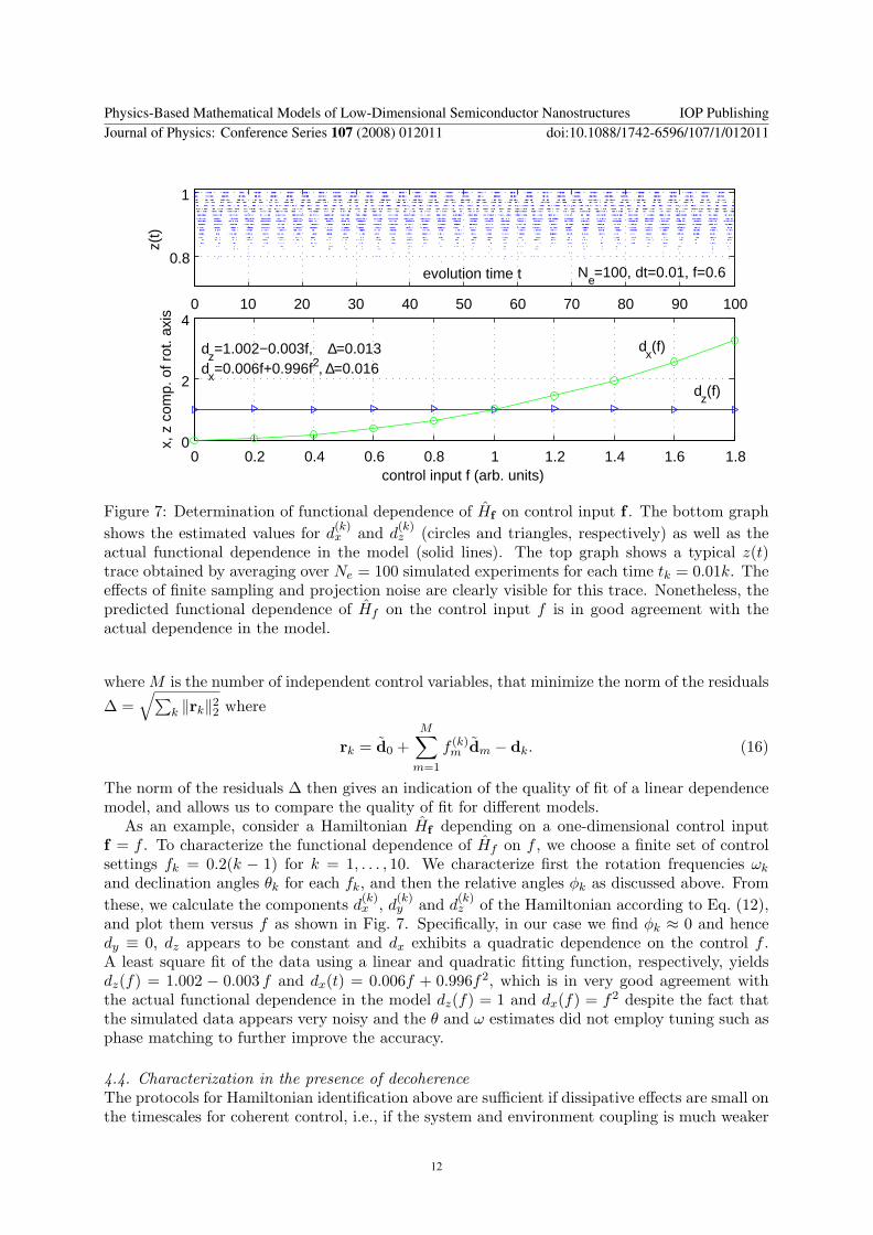
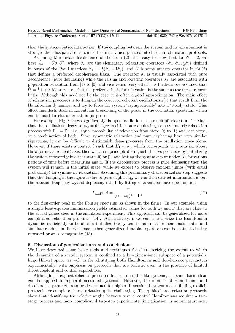
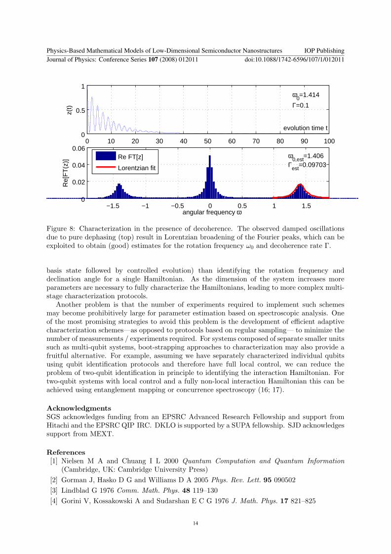