60

RR, SS 2001, ML 2012

Physics 340 Laboratory

Blackbody Radiation: The Stefan-Boltzman Constant Objective: To measure the energy radiated by a blackbody cavity as a function of temperature. References: 1. Experimental Atomic Physics, G.P. Harnwell and J.J. Livingood, McGraw-Hill,

NY (1933), pgs. 50-58. 2. Modern Physics, 2nd Edition, Kenneth Krane, Wiley and Sons, NY (1996), pgs.

77-83 and pgs. 320-322. 3. Radiation Processes in Astrophysics, G. Rybicki and A.P. Lightman, Wiley-VCH,

NY (1985), Chapter 1. Apparatus: Electrical furnace, NiCr-Ni thermocouple, variac, CASSY interface, computer, water-cooled radiation shield and plastic tubing, Moll’s thermopile. Introduction: Following James Maxwell’s unification of electricity and magnetism in the late 1860’s and his prediction of electromagnetic radiation, an intense effort followed to detect and generate this new type of radiation. After the realization that light itself was an electromagnetic wave, there was an explosion of interest to understand in detail how light was generated. This led to a series of fundamental studies characterizing many different types of light sources. The results of these studies were so puzzling that they eventually provided the groundwork for the formulation of quantum physics. One subject of particular interest during this time was the characterization of light emitted from a hot object. As known from prehistoric times, any object heated to a high enough temperature emits visible light. As early as 1802, Count Rumford (Benjamin Thompson) suggested that blackening the surface of an object enhanced its thermal radiative properties. Consequently, the radiation emitted from a well-characterized object like a hollow cavity came to be known by a variety of names such as blackbody radiation, temperature radiation, or cavity radiation. It was discovered that such radiation depends only on the temperature of the cavity and this fact differentiates it from other types of radiation such as that emitted from a glow discharge tube. It was quickly realized that blackbody radiation emitted in the visible region of the electromagnetic spectrum only becomes appreciable when the temperature of the cavity is above 500-550 °C (about 800-850 K). Blackbody radiation emitted at lower temperatures had to be detected by other than optical means.

61

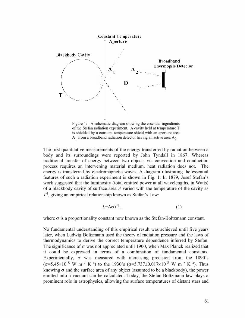
Figure 1: A schematic diagram showing the essential ingredients of the Stefan radiation experiment. A cavity held at temperature T is shielded by a constant temperature shield with an aperture area A1 from a broadband radiation detector having an active area A2.

The first quantitative measurements of the energy transferred by radiation between a body and its surroundings were reported by John Tyndall in 1867. Whereas traditional transfer of energy between two objects via convection and conduction process requires an intervening material medium, heat radiation does not. The energy is transferred by electromagnetic waves. A diagram illustrating the essential features of such a radiation experiment is shown in Fig. 1. In 1879, Josef Stefan’s work suggested that the luminosity (total emitted power at all wavelengths, in Watts) of a blackbody cavity of surface area A varied with the temperature of the cavity as T4, giving an empirical relationship known as Stefan’s Law: L=AsT4 , (1) where s is a proportionality constant now known as the Stefan-Boltzmann constant. No fundamental understanding of this empirical result was achieved until five years later, when Ludwig Boltzmann used the theory of radiation pressure and the laws of thermodynamics to derive the correct temperature dependence inferred by Stefan. The significance of s was not appreciated until 1900, when Max Planck realized that it could be expressed in terms of a combination of fundamental constants. Experimentally, s was measured with increasing precision from the 1890’s (s=5.45´10-8 W m−2 K−4) to the 1930’s (s=5.737±0.017´10-8 W m−2 K−4). Thus knowing s and the surface area of any object (assumed to be a blackbody), the power emitted into a vacuum can be calculated. Today, the Stefan-Boltzmann law plays a prominent role in astrophysics, allowing the surface temperatures of distant stars and

62

planets to be inferred from measurements of their distances and apparent brightnesses. In this experiment, you will repeat Stefan’s measurements using computer-assisted data acquisition techniques and you will obtain an estimate for the Stefan-Boltzmann constant s. Theory: At the close of the nineteenth century, a major unresolved problem in classical physics involved a major discrepancy between the predicted spectrum of a blackbody and what was actually observed in the lab. By using Maxwell’s equations and the laws of thermodynamics, Lord Rayleigh had derived that a blackbody spectrum (the energy emitted per unit frequency) should vary as ν4T, where ν is the observed photon frequency. This prediction held true for low frequencies, but unfortunately it predicted that an ever increasing number of photons would be produced at the highest frequencies (the so-called ‘ultraviolet catastrophe’). In late 1900, Max Planck came upon a brilliant solution to the problem, by making a crucial modification to the blackbody model. Whereas Rayleigh had described the photons inside a blackbody cavity as standing waves with nodes at the cavity walls, each with equal energy kT, Planck suggested that the energies of the standing waves were in fact quantized, and were integer multiples of hc/λ, where h is Planck’s constant (6.62606957(29)×10−34 J s). Thus, at high frequencies (i.e., short wavelengths such as ultraviolet), each photon carried significantly more energy, and since photons will tend to occupy the lowest energy states first according to statistical mechanics, comparatively few UV photons will be produced for a given amount of thermal energy available in the blackbody cavity. This solution to the ultraviolet catastrophe cemented the failure of classical physics as a complete description of nature and was instrumental in launching the modern era of quantum mechanics. Planck’s formulation involved a consideration of the density of quantum states available to the photons in the blackbody cavity per unit frequency interval. To derive the average energy per photon state he used the Boltzmann factor (e-E/kT) and his quantum wave energy hν. Multiplying all these quantities together, and accounting for two possible polarizations of the photons, his predicted blackbody spectrum was

, (2)

which is now known as the Planck function (a more comprehensive derivation can be found in the list of references accompanying this write-up). In this experiment you will be measuring two main properties of a blackbody: its internal temperature (using the thermocouple), and its emitted radiation field (using the thermopile). The latter is traditionally described using such quantities as specific

)1(2

/2

3

-= kThec

hB nnn

63

intensity (brightness), flux, and luminosity. We have already defined luminosity as the total energy output of a blackbody over all frequencies. This is typically impossible to measure in the lab, as it would require you to capture and record every single photon emitted. Instead you will be observing the blackbody radiation (in our case, from an oven) that escapes through a small aperture of area A1, using a thermopile having an opening aperture area A2 , located a distance D away (Figure 1). It is convenient to describe the measured energy dE from a small bundle of light rays crossing a small aperture of area dA in a time dt in terms of a specific intensity Iν, which is defined such that

. (3)

In this formulation the directions of all the rays lie within a small solid angle dΩ , are approximately perpendicular to the aperture dA, and have photon frequencies lying within a small range dν. The solid angle is the two-dimensional equivalent of a standard angle, and refers to the apparent area subtended by an object. For example, the Moon has an apparent radius of 0.25 degrees (4.36 x 10-3 radians) as seen from Earth, and thus subtends π (4.36 x 10-3)2 = 6 x 10-5 steradians on the sky. Eq. (3) provides the definition of specific intensity Iν (often called brightness) in units of W m-2 Hz-1 steradian-1, and pertains to rays propagating only along a very narrow direction. In real life however, glowing objects emit rays in all directions, many of which will make it to our detector. Imagine you set up a small flat aperture of small area dA whose normal lies at some angle θ to the surface of a blackbody as in Figure 2. Then we can define the radiative flux from the blackbody as

, (4) which in spherical coordinates becomes

. (5)

You may notice that flux is an observer-based quantity, since to evaluate the right hand side, we integrate the brightness of the object over all possible directions – however Iν is non-zero only along those directions where our line of sight intercepts the object. In other words, if we move the object farther away, its solid angle (and therefore its flux) decreases as 1/D2, giving rise to the familiar inverse-square law for light.

nn dddtdAIdE Wº

W=ò dIF qnn cos

fqqqp

f

p

q nn ddIF sincos2

0 0ò ò= ==

64

Figure 2. Sketch showing the geometry used in the definition of radiative flux. The effective area of the detector is proportional to the cosine of the observation angle θ. The blackbody subtends an apparent angular radius θc = sin-1(R/D).

To illustrate this effect, imagine locating your detector a distance D from a spherical blackbody of radius R and uniform surface intensity I (let’s assume that your detector can receive all photon frequencies, and has its normal vector pointing directly at the blackbody). According to Eq. (5), the measured flux will be

(6)

where from simple geometry, θc = sin-1(R/D) is the apparent angular radius of the blackbody. Performing the integration gives

(7)

Thus for a fixed spherical blackbody of surface intensity I and radius R, the flux varies as 1/D2, confirming the inverse-square law of light. We can now use Eq. (7) to derive the flux per unit area radiating from the surface of a spherical blackbody by setting R = D:

. (8) Multiplying this by the surface area A of the blackbody yields its total luminosity:

. (9)

Comparing this with Eq. (1), we can see that for a spherical blackbody

. (10)

Blackbody

θ

dA

D

normal R

θc

,sin2

0 0qqqf

p

f

q

qdoscdIF c

ò ò= ==

.2

÷øö

çèæ=DRIF p

IF p=

IAL p=

ps 4TI =

65

Now according to Planck’s radiation law, the left hand side of Eq. (10) should be equivalent to Planck’s function Bν (Eq. 2) integrated over all photon frequencies. An integration of Eq. (2) by parts gives the predicted blackbody luminosity per unit surface area:

. (11)

Comparing this to Eq. (10), we find that the Stefan-Boltzmann constant is in fact a combination of several other fundamental constants:

, (12)

which has an experimentally determined value of 5.670373(21)×10−8 W m−2 K−4. In practice, any object (not necessarily a hollow cavity) heated to a temperature T emits radiation. Experiment shows that the maximum power radiated per unit area comes from a cavity and is specified by Eq. (2). The emitted luminosity per unit area of any arbitrary object held at temperature T is specified by the non-ideal blackbody formula

L = esT4 , (13) where e is known as the emissivity of the emitting object. By definition, an ideal blackbody has e=1. Every material has a characteristic emissivity; for instance, tungsten has e=0.2. Experimental Considerations: It is difficult to accurately measure the total emissive power radiated from a blackbody. This would require a detector that collects the radiation emanating from the blackbody in all directions. In general, only a small fraction of the emitted energy can be collected. Therefore, careful attention must be paid to the geometrical arrangement of the blackbody and detector in order to allow a correct interpretation of the data. Also, careful measurements must take into account any energy absorbed by the intervening air column, which can be difficult to control if air conditioners or fans are continually circulating air through the laboratory room. In addition, a broad-band detector must be designed to accurately measure the incident power over a wide range of wavelengths. In this experiment, you will use a thermopile to accomplish this function. A thermopile is a blackened disk of known dimension that is thermally anchored to a series of thermocouple junctions. A thermocouple is a junction formed when two wires, each made from a dissimilar metal, are joined together in an intimate fashion. A thermocouple junction is known to develop a voltage across it that depends on temperature. In this way, the temperature of the disk can be measured in terms of a voltage difference that

32

444

152

hcTkB p

=

32

45

152

hckps =

66

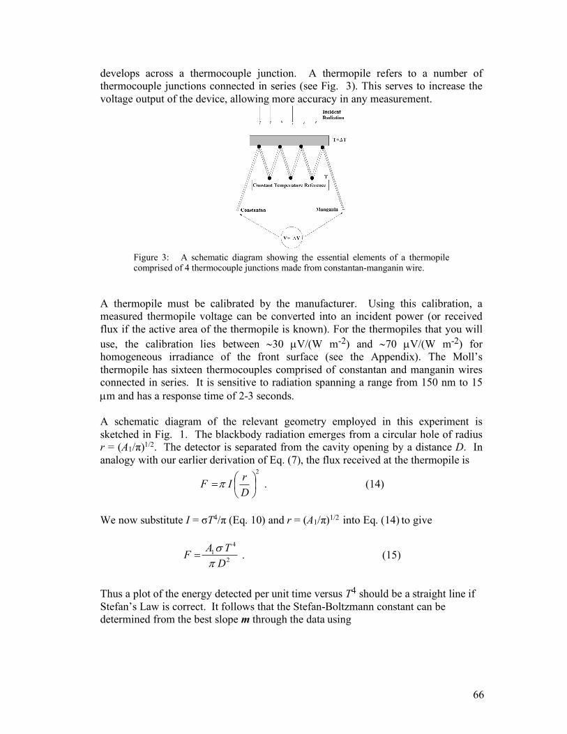
develops across a thermocouple junction. A thermopile refers to a number of thermocouple junctions connected in series (see Fig. 3). This serves to increase the voltage output of the device, allowing more accuracy in any measurement.

Figure 3: A schematic diagram showing the essential elements of a thermopile comprised of 4 thermocouple junctions made from constantan-manganin wire.

A thermopile must be calibrated by the manufacturer. Using this calibration, a measured thermopile voltage can be converted into an incident power (or received flux if the active area of the thermopile is known). For the thermopiles that you will use, the calibration lies between ~30 µV/(W m-2) and ~70 µV/(W m-2) for homogeneous irradiance of the front surface (see the Appendix). The Moll’s thermopile has sixteen thermocouples comprised of constantan and manganin wires connected in series. It is sensitive to radiation spanning a range from 150 nm to 15 µm and has a response time of 2-3 seconds. A schematic diagram of the relevant geometry employed in this experiment is sketched in Fig. 1. The blackbody radiation emerges from a circular hole of radius r = (A1/π)1/2. The detector is separated from the cavity opening by a distance D. In analogy with our earlier derivation of Eq. (7), the flux received at the thermopile is

. (14)

We now substitute I = σT4/π (Eq. 10) and r = (A1/π)1/2 into Eq. (14) to give

. (15)

Thus a plot of the energy detected per unit time versus T4 should be a straight line if Stefan’s Law is correct. It follows that the Stefan-Boltzmann constant can be determined from the best slope m through the data using

2

÷øö

çèæ=DrIF p

2

41

DTAF

ps

=

67

. (16)

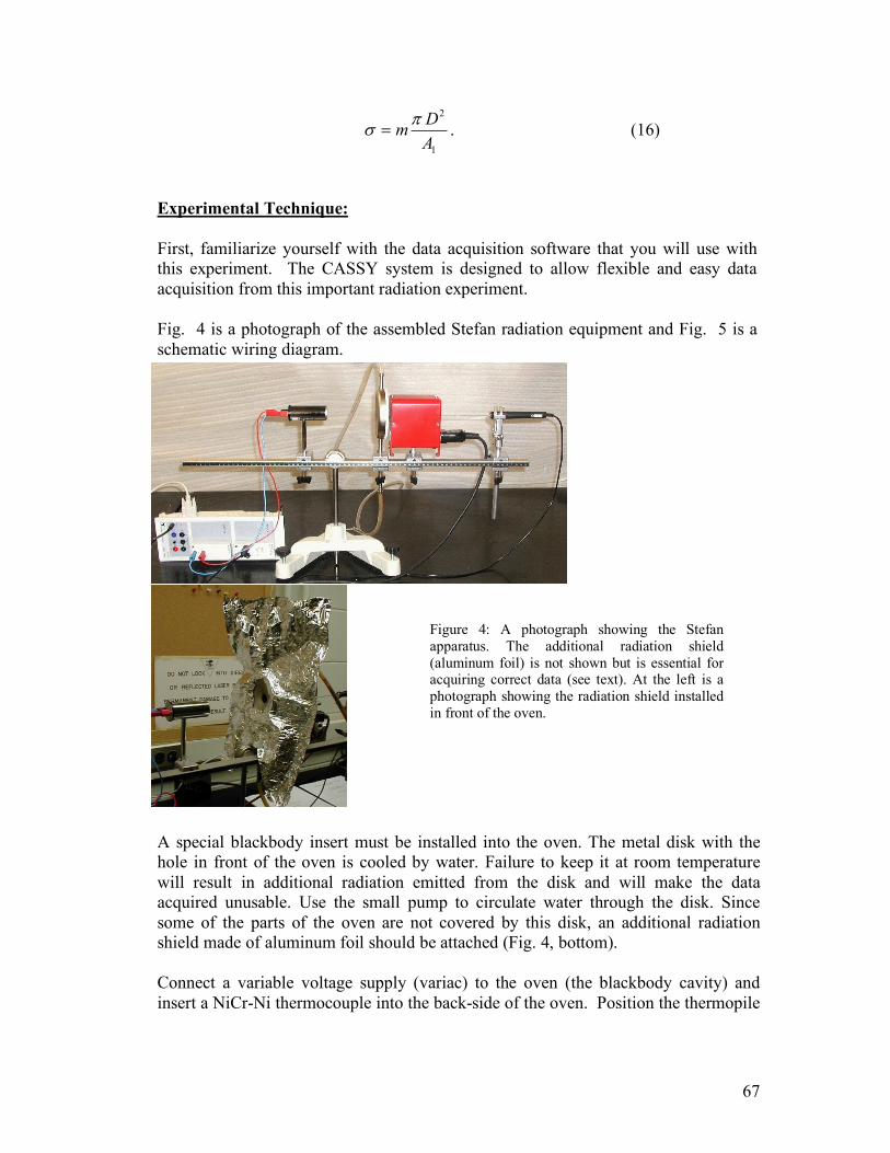
Experimental Technique: First, familiarize yourself with the data acquisition software that you will use with this experiment. The CASSY system is designed to allow flexible and easy data acquisition from this important radiation experiment. Fig. 4 is a photograph of the assembled Stefan radiation equipment and Fig. 5 is a schematic wiring diagram.

A special blackbody insert must be installed into the oven. The metal disk with the hole in front of the oven is cooled by water. Failure to keep it at room temperature will result in additional radiation emitted from the disk and will make the data acquired unusable. Use the small pump to circulate water through the disk. Since some of the parts of the oven are not covered by this disk, an additional radiation shield made of aluminum foil should be attached (Fig. 4, bottom). Connect a variable voltage supply (variac) to the oven (the blackbody cavity) and insert a NiCr-Ni thermocouple into the back-side of the oven. Position the thermopile

1

2

ADmps =

Figure 4: A photograph showing the Stefan apparatus. The additional radiation shield (aluminum foil) is not shown but is essential for acquiring correct data (see text). At the left is a photograph showing the radiation shield installed in front of the oven.

68

approximately 0.15 m in front of the oven. Make sure that the protective glass cover is removed from the entrance of the thermopile.

Figure 5: A schematic wiring diagram for the Stefan apparatus. Data Acquisition Procedure: (a) Note the manufacturer’s serial number of your thermopile, and then record its output voltage with the oven at room temperature. At this time, make sure you know how to acquire data with the CASSY system. This measurement serves as the zero-point reference for all your future measurements. Set the distance D between the detector and the cavity opening to about 0.15 m. Measure the diameter of the cavity opening and calculate its area (A1). Also, be sure you write down the ambient temperature of the room. (b) Set up the CASSY system to record the oven temperature and the thermopile voltage. Set the display to show temperature as x-axis and thermopile voltage as y-axis. Set the measurement interval to 500 ms and the recording condition to n=1 or delta(&JA11)>2 (the command is case sensitive). The latter condition means that the measurement should be taken only when the first point is acquired (n=1) or when temperature (&JA11) increases by 2. See that the number of points to be accumulated is left blank, or set it to maximum possible value. Also, set the measurement mode to Average 100 ms for both temperature and voltage detector. This serves to minimize the effects of short-timescale voltmeter noise in your measurements.

69

(c) Start the measurement and turn the variac up to ~100 V. At this setting it will take approximately 20 minutes for the temperature to reach 400 °C. At the highest temperatures, the outside of the oven is very HOT, so do not touch it without oven mitts. The data will be accumulated automatically. (d) When the oven temperature reaches a constant temperature of approximately 400 °C, stop the measurement and decrease the variac voltage to ~90V. Save the data you just acquired. (e) See that the temperature stabilizes at ~400 °C, tune the variac voltage slightly down if temperature keeps rising, or up if it goes down (by few volts). Note that it may take a minute or so before changes in voltage reflect in temperature change. Once the temperature is reasonably stable, make a series of measurements in which you vary the distance between the thermopile and the entrance to the blackbody. Be sure to cover distance between ~5 cm to the full length of the rail and acquire about 20 points. Remember to wait after each move before you take the measurement as the detector has long time constant. (f) Choose another distance (greater than the 0.15 m used in step (b)) between the thermopile and the entrance to the blackbody. Set up the measuring condition to n=1 or delta(&JA11)<-2. Start new data acquisition (the previously accumulated data will be cleared automatically), set the variac to zero, and then turn off the variac. The new set of data will be recorded as the oven returns to room temperature. (g) When you are finished, make sure you turn off the cooling water, replace the protective glass cover over the entrance of the thermopile, and copy any useful data onto a thumb drive or your network account for further analysis. Data Analysis: (a) Analyze your data as function of distance between the thermopile and the entrance to the blackbody. How well does it follow a D-2 relationship expected from Eq. 16? For what values of D would you expect a D-2 behavior to accurately hold? For each distance, calculate the value of s using Eq. 16. Plot your calculated value of T as a function of distance. What can you say about this graph? (b) Analyze your data as a function of temperature during the warming phase of the oven. Remember to correct your data for the energy radiated away from the thermopile detector at room temperature. This requires you to plot Fin(T)-Fin(TRT) vs. (T4-TRT

4) , where TRT is the temperature of the room. From this plot, measure the slope and extract an estimate for the Stefan-Boltzmann constant. Alternatively, you may analyze the original data using Eq. 16, and estimate the value of s from that. Calculate the value of s for several temperatures and plot s versus T. Is it constant? If not, what might be the reason?

70

(c) In the same way, analyze your data as a function of temperature during the cooling phase of the oven. (d) Tabulate your two estimates of s in a clear way. What is your best estimate for the Stefan-Boltzmann constant? Make sure you include a realistic discussion of errors in your measurements of A1 and D. What is the resulting uncertainty in s? (e) Discuss any significant sources of unaccounted error that you believe are relevant to this experiment. Is it possible that these errors account for the difference between your measured value of s and the accepted value?

Appendix: Moll’s Thermopile Calibrations

Manuf. Specs. Calibrated by SS (Fall 2001)

Serial No. 999415: 35.5 µV/(W m-2) 52±5 µV/(W m-2) Serial No. 009561: 44.3 µV/(W m-2) 66±5 µV/(W m-2) Serial No. 009562: 63.4 µV/(W m-2) 92±5 µV/(W m-2) Serial No. 009576: 39.7 µV/(W m-2) 59±5 µV/(W m-2)