physics 239 (211c): quantum phases of matter spring 2021
TRANSCRIPT

Physics 239 (211C): Quantum phases of matter
Spring 2021
Lecturer: McGreevy
These lecture notes live here. Please email corrections and questions to mcgreevy at
physics dot ucsd dot edu.
Last updated: June 7, 2021, 15:04:48
1

Contents
0.1 Introductory remarks and goals . . . . . . . . . . . . . . . . . . . . . . 3
0.2 Conventions . . . . . . . . . . . . . . . . . . . . . . . . . . . . . . . . . 4
0.3 Sources . . . . . . . . . . . . . . . . . . . . . . . . . . . . . . . . . . . . 5
1 Defects and textures of ordered media 6
1.1 Landau-Ginzburg theory of ordering . . . . . . . . . . . . . . . . . . . . 6
1.2 When are there stable defects? . . . . . . . . . . . . . . . . . . . . . . . 12
1.3 The vacuum manifold . . . . . . . . . . . . . . . . . . . . . . . . . . . . 16
1.4 Examples . . . . . . . . . . . . . . . . . . . . . . . . . . . . . . . . . . 18
1.5 Homotopy groups of symmetric spaces . . . . . . . . . . . . . . . . . . 24
1.6 When π1(V ) is non-abelian . . . . . . . . . . . . . . . . . . . . . . . . . 29
1.7 Textures or solitons . . . . . . . . . . . . . . . . . . . . . . . . . . . . . 33
1.8 Defects of broken spatial symmetries . . . . . . . . . . . . . . . . . . . 34
1.9 The boojum and relative homotopy . . . . . . . . . . . . . . . . . . . . 44
2 Some quantum Hall physics 46
2.1 Electromagnetic response of gapped states in D = 2 + 1 . . . . . . . . . 48
2.2 Abelian Chern-Simons theory . . . . . . . . . . . . . . . . . . . . . . . 53
2.3 Representative wavefunctions . . . . . . . . . . . . . . . . . . . . . . . 62
2.4 Composite fermions and hierarchy states . . . . . . . . . . . . . . . . . 70
3 Symmetry-protected topological phases 79
3.1 EM response of SPT states protected by G ⊃ U(1) . . . . . . . . . . . . 82
3.2 Anomaly inflow and fermion zeromodes on topological defects . . . . . 93
3.3 Coupled-layer construction . . . . . . . . . . . . . . . . . . . . . . . . . 111
3.4 Wavefunctions for SPTs . . . . . . . . . . . . . . . . . . . . . . . . . . 116
3.5 Spin structures and fermions . . . . . . . . . . . . . . . . . . . . . . . . 125
3.6 Characteristic classes and classifying spaces . . . . . . . . . . . . . . . 128
3.7 Classification of SPTs, part one . . . . . . . . . . . . . . . . . . . . . . 132
3.8 Global anomaly inflow . . . . . . . . . . . . . . . . . . . . . . . . . . . 134
3.9 Classification of SPTs, part two . . . . . . . . . . . . . . . . . . . . . . 138
2

0.1 Introductory remarks and goals
The study of phases of matter is a topology problem. We wish to divide the set
macroscopic piles of stuff, with some interactions
into equivalence classes. The equivalence relation is roughly: two interacting piles of
stuff are regarded as being in same phase if their observable properties are adiabatically
connected under varying the interactions and adding in more non-interacting, gapped
stuff. So phases of matter are essentially elements of π0(piles of stuff). 1
A topological invariant is a quantity that does not change under such continuous
variations, for example a quantity that is guaranteed to be an integer. Such invariants
are wonderful because they provide labels on our equivalence classes. The simplest
example of a topological invariant labelling a phase of matter is the (integer!) number
of groundstates of an Ising magnet: it is 2 in the ordered phase, and 1 in the disordered
phase; thus these two phases must be distinct. So you see that the use of topology in
condensed matter physics is not just for ‘topological phases’.
Topological phases are those that are distinguished from others, say from the trivial
state, by properties other than ordinary symmetry breaking. (A good representative
of the trivial state is an atomic insulator, where each particle is 600 miles from its
nearest neighbor and never even says ‘hello’. More generally, the trivial phase is one
that has a product state representative that breaks no symmetries.) By now there is
a large variety of known ways in which phases can be topological, some of which are
pretty fancy mathematically. Some of them have even been found in Earth rocks. My
main goal in this course will be to try to explain some of these phenomena, and the
topologically-invariant labels we can attach to them, as concretely as possible.
Last quarter we developed some tools of algebraic topology, at least some such tools
that are realized in toy models of physical systems. I know that not all of the members
of this class took last quarter’s class. I am going to do my best to make our discussion
here self-contained while at the same time avoiding repetition. At times I may have to
ask those of you who are just joining us to do some extra background reading or take
some statements on faith. To help clarify what topics I’m not going to repeat, I’ve
posted a summary of the mathematical highlights; I don’t expect you to absorb every
detail of this, but rather to use it as a resource as needed.
Conversely, I think not everyone took the previous two quarters of the condensed
matter series. If it seems like I am assuming some knowledge you don’t have please do
not hesitate to ask.
1πq of this space for q > 0 is also interesting but much less well-explored so far.
3

For a list of topics we might cover, see the table of contents of this document, or
this administrative handout.
0.2 Conventions
For some of us, eyesight is a valuable and dwindling commodity. In order not to waste
it, I will often denote the Pauli spin operators by
X ≡(
0 1
1 0
)Y ≡
(0 −i
i 0
)Z ≡
(1 0
0 −1
)(rather than σx,y,z, which hides the important information in the superscript) in the Z
basis. I’ll write |0〉, |1〉 for the Z eigenstates, Z |0〉 = |0〉 and Z |1〉 = − |1〉 and |±〉 for
the states with X |±〉 = ± |±〉.
I use ijk for spatial indices, µνρ for spacetime indices. d is the number of space
dimensions and D = d+ 1 is the number of spacetime dimensions (it’s bigger).
≡ means ‘equals by definition’. A!
= B means we are demanding that A = B.
A?= B means A probably doesn’t equal B.
The convention that repeated indices are summed is always in effect unless otherwise
indicated.
A useful generalization of the shorthand ~ ≡ h2π
is
dk ≡ dk
2π.
I will also write /δ(q) ≡ (2π)dδd(q).
I try to be consistent about writing Fourier transforms as∫ddk
(2π)deikxf(k) ≡
∫ddk eikxf(k) ≡ f(x).
WLOG ≡ without loss of generality.
IFF ≡ if and only if.
RHS ≡ right-hand side. LHS ≡ left-hand side. BHS ≡ both-hand side.
IBP ≡ integration by parts.
+O(xn) ≡ plus terms which go like xn (and higher powers) when x is small.
iid ≡ independent and identically distributed.
We work in units where ~ and kB are equal to one unless otherwise noted.
Please tell me if you find typos or errors or violations of the rules above.
4

0.3 Sources
This list will grow with the notes.
N. Mermin, The Topological Theory of Defects in Ordered Media
G. Volovik, Exotic properties of superfluid 3He.
M. Nakahara, Geometry, Topology and Physics. I was not a big fan of this book when
I was a student because I thought it was superficial. Looking at it again now, I
see its virtues more clearly. It has useful things in it and it is mostly written for
physicists.
Nash and Sen, Geometry and Topology for Physicists. This book has the virtue of
brevity.
D. Tong, Lectures on the Quantum Hall Effect.
X.-G. Wen, Quantum Field Theory of Many-Body Systems, Oxford, 2004.
X.-G. Wen, Topological orders and Edge excitations in FQH states.
A. Zee, Quantum Hall Fluids.
G. Moore, Quantum Symmetries and Compatible Hamiltonians.
G. Moore, Introduction to Chern-Simons Theories.
J. Harvey, Lectures on Anomalies.
E. Witten, Three Lectures On Topological Phases Of Matter.
E. Witten, Fermion Path Integrals And Topological Phases.
A. Turner and A. Vishwanath, Beyond Band Insulators: Topology of Semi-metals and
Interacting Phases.
T. Senthil, Symmetry Protected Topological phases of Quantum Matter.
C. Z. Xiong, Classification and Construction of Topological Phases of Quantum Mat-
ter.
5

1 Defects and textures of ordered media
[Mermin, Nash and Sen’s disappointing §9, Nakahara’s disappointing §4.8-4.10, Volovik,
Exotic properties of superfluid 3He, §2]
The subject we are about to discuss was developed in the 1970s, apparently in
response to the amazing discoveries of the low-temperature phases of 3He. Perhaps
you can regard this as an old subject, then. But, as we’ll see, the understanding we’ll
find and more importantly the perspective we’ll develop is essential background for
more modern questions about quantum phases of matter.
It will also give us a physical and friendly context in which to get everyone up to
speed about homotopy groups.
1.1 Landau-Ginzburg theory of ordering
Suppose we have a many-body system with a symmetry G. To have a definite example
in mind, say G = U(1); this is the symmetry of a planar magnet, or of a collection
of particles with a conserved particle number. The system has at least two possible
phases: G can be unbroken, or it can be spontaneously broken. The latter means that
the equilibrium states are not invariant under G. In that case, the equilibrium states
comprise an orbit of G.
For example, suppose we are speaking about quantum groundstates, zero tempera-
ture. Then the statement that there is a U(1) symmetry means that there is a charge Q
that commutes with the hamiltonian H, [H,Q] = 0. The statement that the symmetry
is spontaneously broken means that given some groundstate |ψ0〉, the symmetry takes
it to
eiQφ |0〉 = |φ〉 ,
another groundstate. Since [H,Q] = 0, the states |φ〉 are energy eigenstates with the
same energy for all choices of φ. Now let’s further assume that the conserved charge is
an integral of a local density:
Q =
∫space
ddx j0(x)
and consider the state
|φ(x)〉 ≡ ei∫space d
dxj0(x)φ(x) |0〉 .
Since when φ is constant, this is a groundstate, |φ(x)〉, must have an energy above
the groundstate (expectation value of the Hamiltonian) proportional to ~∇φ. The idea
is just that E[φ] = 〈φ(x)|H |φ(x)〉 is a nice functional of φ. It is local, meaning a
6

single integral over space, if H is local. Therefore, long-wavelength fluctuations of the
vacuum parameter φ describe low-energy excitations of the ordered phase. This is
the essence of Goldstone’s theorem, and it applies any time a continuous symmetry is
spontaneously broken.
Having just used quantum mechanics language to remind us about Noether and
Goldstone, actually for the rest of this section everything I will say will be just as
relevant and interesting for classical systems – say, equilibrium statistical mechanical
problems with real Boltzmann weights. In fact, at some points I will ignore possible
complex phases that could arise in quantum systems. These will be an interesting
subject for later in the course.
Some variables which make manifest all that I’ve said so far for the case G =
U(1) are the following. Introduce Φ(x) ∈ C, the order parameter field, on which the
symmetry G = U(1) acts linearly Φ 7→ eiαΦ. For example in the case of a planar
magnet, Φ(x) = Sx(x) + iSy(x) is made from the (coarse-grained) local magnetization.
We can associate an energy (or free energy at finite T ) to each configuration of Φ:
FLG[Φ] =
∫space
ddx(V (|Φ|) + κ~∇Φ? · ~∇Φ + terms with more derivatives
)(1.1)
In this expression for the Landau-Ginzburg free energy, we assumed Φ to be slowly-
varying compared to some microscopic scale, such as a lattice spacing, so that terms
with fewer derivatives are more important. Also, this works best if Φ is not too large,
so that terms with fewer powers of Φ are also more important, so we can expand
V (|Φ|) = r|Φ|2 + u|Φ|4 + · · · .
(Φ will not want to be too large if r is not too large and negative.) The crucial
Landau-Ginzburg-Wilson principle by which I decided what terms to write is: I just
wrote all local terms invariant under G, organized by decreasing importance in the
derivative expansion, and I made up names for their coefficients. ‘Local’ here means
that they are written as a single integral over space. Once you believe that F is a
local functional, what else could it be? (I’ll resist the temptation to do dimensional
analysis and write all the coefficients in terms of the energy scales in the problem and
dimensionless numbers.)
One way to motivate this functional and to meaningfully estimate the coefficients
in (1.1) is by mean field theory. One of many ways to describe MFT is: we make an
ansatz for the groundstate wavefunction (or equilibrium density matrix) in the form of
a product state |Φ〉 = ⊗x |Φ(x)〉x, where Φ(x) determines the wavefunction of a single
site. Then use this as a variational wavefunction, and F [Φ] ∼ 〈Φ|H|Φ〉, which we are
then motivated to minimize.
7

For r > 0, V (|Φ|) has a unique minimum at Φ = 0; this is the unbroken
phase.
If r < 0, V (|Φ|) has a circle of minima at |Φ| = v, parametrized by the
angle φ in Φ = veiφ.
So you see that near r = 0 there is some kind of non-adiabatic phenomenon, a
mean-field theory approximation to a phase transition. Near the phase transition, our
assumptions about the locality of the long-wavelength action (or our mean field ansatz
for the wavefunction) break down because Φ itself becomes gapless. Below the upper
critical dimension, this is a real loophole; how to deal with this is a victory of the
renormalization group, not our subject. We’re going to spend the next big chunk of
these notes firmly ensconced in the ordered phase.
If we expand the LG free energy about such an ordered configuration, we find
FLG[Φ = veiφ(x)] =
∫space
(ρ(~∇φ)2 + terms with more derivatives
).
Notice that there is no potential for the goldstone field φ(x). (In contrast, if we allow
fluctuations away from the circle of minima, Φ = (v + δv(x))eiφ(x), the field δv(x)
has a big honking restoring force, (δv(x))2.) On the other hand, gradients of φ cost
energy. This is the phenomenon of generalized rigidity: the nonzero coefficient of (~∇φ)2
measures the (free) energy cost of straining the order by inhomogeneous distortions.
This is absent in the disordered state.
Vortices. Now draw a two-dimensional cross-section of space, and draw in it a
loop C, parametrized as xi(s), with s ∈ [0, 2π). And for a given configuration of the
order parameter field φ(x), consider the quantity
2πw[C] ≡∮C
dφ =
∮C
∂φ
∂xidxi =
∫ 2π
0
∂φ
∂xidxi
dsds = φ(x(s))|2π0 ∈ 2πZ.
We used the chain rule a bunch of times. Since the variable φ ∼= φ + 2π is only well-
defined modulo addition of 2π times an integer, it need not take the same value at the
beginning and the end of the curve.
Now, still for a fixed configuration φ(x), consider what happens as I shrink the
curve C. Since w[C] is always an integer, it can only change by jumping. When it
8

jumps, we say that we have crossed a vortex. This is a locus where φ is singular, not
well-defined. In terms of the definition of φ as the phase of the field Φ, it is clear what
must happen: Φ = 0 in the core of the vortex, so its phase φ is not well-defined. Since
it is defined as a thing a loop can wind around, a vortex is always codimension two,
meaning that its location is specified by two coordinates. If d = 2, a vortex is a point
defect; in d = 3, it is a string defect.
Thinking still about a two-dimensional cross-section of space, a useful perspective
then is that φ defines a smooth map
φ : R2 \ vortices→ S1.
In the case where there is just a single vortex, R2 \point deformation retracts to S1. So
such maps are classified by the fundamental group of S1, [φ] ∈ π1(S1) = Z. w stands
for ‘winding’ – it counts how many times the map winds around the vacuum manifold.
To see some examples of interesting configurations, put polar coordinates on the
two-dimensional cross section of space in question, z = x + iy = reiϕ. Note that
ϕ ≡ ϕ + 2π. If we take φ = φ0, a constant, then w[C] = 0 for any curve, no winding.
If we set φ = φ0 + nϕ, then 2πw[unit circle] =∮Cdφ =
∫ 2π
0dφdϕdϕ = n
∫ 2π
0dϕ = 2πn. n
must be an integer so that φ is single-valued under a 2π rotation in space ϕ ≡ ϕ+ 2π.
Here are configurations with n = +1 (vortex) and n = −1 (antivortex) respectively:
Brief comment on energetics. Our focus here is on the topology, but I have
to mention the following. First, if you plug in the configuration φ = ϕ to the action∫d2x(∂φ)2, you will find an answer that goes like log(L), where L is the size of the
box, not finite energy in the thermodynamic limit. This bitter reality does not do that
much to diminish the utility of these objects: a well-separated vortex-antivortex pair
has finite energy2.
Second, there can always be large energy barriers between various configurations,
which are nevertheless not topologically distinct.
2Also, a finite-energy configuration with the same features occurs in the model where Φ is coupled
to a U(1) gauge field. The model we’ve been discussing so far is a model of a superfluid; the model
where the U(1) is gauged (the abelian Higgs model) is a model of a superconductor. Superconductors
have finite-energy vortices.
9

While we’re at it, let me make a comment about methodology here. When presented
with a functional like FLG[Φ], a physicist has a hard time resisting the urge to extremize
it. Resist the temptation here. Finding a solution of the equations of motion for some
particular choice of coefficients in the expansion of FLG[Φ] is both harder and less
informative than what we are doing. This is because that solution may or may not
be stable to deformations of either the configuration or the coefficients in FLG[Φ]. On
the other hand, once we show that a stable defect is guaranteed by topology, because
it carries some topological invariant (e.g. a homotopy class) different from that of the
uniform configuration, then we can later confidently try to find a representative that
solves the equations of motion away from the core of the defect.
It is interesting to ask what is the winding number w in terms of the order parameter
field Φ. We can write the integrand as dφ = −12iΦ?dΦ + 1
2idΦ?Φ, and therefore for a
big circle of radius R, CR,
2πw[CR] =
∮CR
dφ =
∫r<R
d
(−1
2iΦ?dΦ +
1
2idΦ?Φ
). (1.2)
Since this number is (2π times) the number of vortices in the region r < R, we can
interpret
jv0(x) =1
2πεij∂i
(−1
2iΦ?∂jΦ +
1
2i∂jΦ
?Φ
)as the density of vortices at x.
[End of Lecture 1]
It is also interesting to compare this expression with the conserved charge associated
with the symmetry Φ→ eiαΦ. To speak about conservation laws, let’s allow for time-
dependent configurations, and consider an action S[Φ] =∫ddxdt∂tΦ
?∂tΦ−∫dtFLG[Φ]3.
The amount of charge in a region is then
Q[R] =
∫R
j0
where jµ = −12iΦ?∂µΦ + 1
2i∂µΦ?Φ is the associated Noether current. The equations of
motion for Φ imply (Noether’s theorem) that ∂µjµ = 0, so Q[R] only changes by the
current leaving through the boundary of the region.
Similarly, we can write down a conserved vortex current
jvρ =i
2περµν∂µΦ?∂νΦ (1.3)
3This is not the most generic possibility. The non-relativistic term∫ddxdtΦ?i∂tΦ has fewer deriva-
tives.
10

whose time component is the vortex density above. It is conserved (by equality of
mixed partials), but it is not obviously a Noether current.
One more comment about the vortex current density jvρ . What is it in terms of φ?
If you go back to (1.2) and write everything in terms of φ, it is
2πw[CR] =
∮CR
dφ =
∫R
d2φ =1
2
∫R
d2xεij∂i∂jφ = 2π
∫R
d2xjv0(x).
We conclude that the density of vortices is
jv0(x) =1
2εij∂i∂jφ = d2φ. (1.4)
We are used to saying that the exterior derivative squares to zero, d2 = 0. This is
crucial for the definition of cohomology! But it assumes that d is acting on smooth
functions. In the core of a vortex, where Φ = 0, φ is not a smooth function, and
the mixed partials need not (and don’t) commute. On the other hand, Φ is a smooth
function.
Crucial observation: the presence of defect around which w 6= 0 can be detected
by w[C] for some arbitrarily distant curve C, without ever investigating what happens
in the singular region. This means that to repair the singularity (i.e. to remove the
defect) requires a singularity (either this one leaving, or one with the opposite winding
coming in) to pass through all such curves C, no matter how far away. In this sense,
a defect about which w 6= 0 is topologically stable – its stability is protected by the
topological nontriviality of the winding.
In contrast, while a configuration with w[C] = 0 can still be singular,
I claim that any such singularity can be repaired locally. That is,
we can find another configuration that is identical
outside any curve C with w[C] = 0,
but which is continuous in the disk-like region whose boundary is C.
(1.5)
The proof of this statement proceeds from a lemma we’ll prove in the
next subsection.
↓ only making changes
inside the blue region
11

1.2 When are there stable defects?
So you can see that the story of the previous subsection has many possible generaliza-
tions. Let
V ≡ minima of V (Φ)
be the ‘vacuum manifold’ – the space of uniform equilibrium states of (equal) minimal
free energy. In example of the previous subsection, we had V = S1.
Fact: There are no stable topological defects of codimension q if πq−1(V ) = 0.4
Here by ‘πk = 0’ I mean it is the set with just one element.
Walls. What about the case of q = 1?
A codimension-one defect is a domain wall. According to the Fact, these can be
topologically stable when V has multiple connected components.
For example, consider a system with a Z2 symmetry. The
analog of the linearly-transforming field Φ is a real field,
which transforms as Φ → −Φ under the Z2. The Z2 sym-
metry says that V (Φ) contains only even powers of Φ, which
can accommodate a double-well potential, with minima at
Φ = ±v. The two broken-symmetry vacua are mapped to
each other by the action of the symmetry. In this example,
then, V = Z2 has two connected components, and π0(V )
does, too.
A domain wall is a configuration of Φ that starts at one value
on the left and goes to the other value on the right. Notice
that like in the case of a vortex, it hits the disordered value
Φ = 0, where the sign of Φ is ill-defined, in the middle.
4Very briefly,
πk(X, p) ≡ maps, α : Sk → X,α(N) = p/ 'maps from the sphere to V taking the north pole N to the base
point p, modulo homotopy equivalence. The purpose of the base
point p is to allow us to multiply two such maps α, β by the picture
at right:Under this product, πk(V, p) forms a group. The identity is [constant map to the base point]. When
it doesn’t cause trouble, we suppress the dependence on the base point, since different base points
produce isomorphic groups when V is path-connected. πq−1(V ) = 0 means that any such map can be
continuously deformed to the constant map to the base point.
12

Lemma: A continuous map φ : Sn → V is homotopic to a constant map
⇔ φ can be extended to φ : Bn+1 → V , with φ|∂Bn+1=Sn = φ.
The proof is beautifully constructive: In the =⇒ direction, suppose
there exists a homotopy φt : Sn → V, t ∈ I, with φ0 = φ, φ1 = c,
a constant map. Now observe that any y ∈ Bn+1 \ 0 is uniquely
labelled as y = tx, t ∈ I, x ∈ Sn.
So let φ : Bn+1 → V be φ(tx) = φ1−t(x). Notice that φ(0) = φ1 = c is well-defined.
The converse works by reading the previous sentences in reverse order.5
So this lemma shows that one purpose of homotopy groups is to measure the ob-
struction to extending a map from Sn to its ‘interior,’ or more precisely to any ball
whose boundary is Sn.
Proof of fact: Thicken a putative isolated codimension-q de-
fect into a (generalized) cylinder Bq×Rd−q. Now consider the
continuous map φ : space \ defect → V . The goldstone field
φ wants to be continuous because of the gradient terms in
FLG. In particular, we can restrict to a Sq−1 which surrounds
the defect: S = (Sq−1 = ∂Bq, x) for some point x ∈ Rd−q.
Then φ|S : Sq−1 → V represents an element of πq−1(V ) (with some choice of base
point). But if πq−1(V ) = 0, then any such map is homotopic to the constant map.
Therefore, the lemma implies that we can extend φ continuously into the interior of B
with ∂B = S – there is no defect in there!
Now you see that we have a proof of (1.5): Surround the putative singularity with
a closed curve C. By assumption w[C] = 0. This means the map φ : C → V is
homotopic to the constant map. Using this homotopy, f , the configuration φ can be
filled in by a continuous map
φ :B → V
(t, x) 7→ f(tx) = f1−t(x).
Notice that f1(x) is a constant, so this map is continuous.
5Notice that in the =⇒ direction, this argument works also if we replace Sn by some other
manifold Σ, such as a torus Tn. Again a point in the handlebody obtained by filling in the interior of
Σ is uniquely labelled by a point x ∈ Σ and t ∈ I, and we can extend φ by φ(t, x) = φ1−t(x). In the
other direction, it’s no longer true that the locus labelled t = 0 is a single point; indeed for the case
of T 2, the center of the donut is a circle, whose map to V may not be homotopic to a constant map
(if π1(V ) 6= 0). Thanks to Tarun Grover for bringing this up.
13

Now we have to ask: does this mean that πq−1(V ) classifies codimension-q defects?
The answer is ... almost.For definiteness, let’s focus for a bit on codimension-two defects in a
medium with π1(V ) 6= 0. So consider a configuration of φ : Rd → V and
pick C, a closed curve surrounding a (d − 2)-dimensional defect. Then
φ|C : S1 → V specifies an element [α ≡ φ|C ] ∈ π1(V, φ0). Here the base
point φ0 is some point in the image of φ|C that we like.
But if we choose a different map φ, or even draw a different curve γ, there is no
guarantee at all that φ0 lies on the resulting image.
One response to this is to consider configurations such that some
point x0 in space is mapped to the base point φ0 ∈ V . then we
deform our curve C by appending a path δ from x0 to the curve
before and after we traverse C. This addition acts by α→ βαβ−1,
where β = φ(δ). This makes it plausible that codimension-two
defects correspond to conjugacy classes of π1(V ), i.e. π1(V )/(α ∼βαβ−1). Moving the base point around will produce different
elements of the same conjugacy class. If π1(V ) is abelian, this is
the same as elements of π1(V ) and we can forget about it.
[End of Lecture 2]
An alternative way to think about the problem is in terms of free homotopy, where
we don’t have a base point. Think about moving our curve C around in space from C1
to C2. The path we take defines a homotopy between φ(C1) and φ(C2). But these two
loops in V need not share a base point. So more precisely, this defines a correspondence
codimension-two defects ↔ loops in V / ' .
The equivalence relation on the right is free homotopy (not preserving any base point)
so the resulting quotient is not a group.
Two loops f, g are freely homotopic in V if and only if there
exists a path γ connecting x ∈ f to y ∈ g with f ' γgγ−1.
This is because γgγ−1 is freely homotopic to g just by retracting γ:
14

Now let’s think about composite defects. Suppose we have
two (parallel) codimension-two defects labelled by P and Q,
elements of π1(V ) (with some base point φ(x), in the figure).
If we draw a big loop C around both, the order parameter
configuration inside C can be smoothly deformed into any
configuration representing the same homotopy class, which
is in general different from either that of P or Q. But the
path C is homotopic to a path which just goes around P and
Q individually. In fact, we can preserve a base point during
this homotopy. So we can ask: In what order?
Well, a basic fact about groups is that for any two elements a, b ∈ G, ab = a(ba)a−1
so ab and ba are in the same conjugacy class. Phew.
If π1(G) is abelian, as in our example above, the order doesn’t matter, and the
result is just the sum of the winding numbers.
Now let’s talk about defects of larger codimension. We will show that for general
q ≥ 2
codimension-q defects ↔ πq−1(V, p)/π1(V, p). (1.6)
To understand the action of π1 on πq−1 on the RHS (which
for q = 2 is just conjugation), first lets recall why, if V is
path connected, changing the base point gives isomorphic
groups: πk(V, x) ∼= πk(V, y) ≡ πq(V ). The idea is: suppose
we are given a path γ from x to y and a representative f :
(Ik, ∂Ik) → (V, x) of πk(V, x), as at right. We will make a
representative of πk(V, y).
6
6Note that the sphere Sk is homeomorphic to the cube Ik/∂Ik with all points on its boundary
identified with each other:
So a map from the sphere to V taking the north pole to x is equivalent to a map from Ik to V
taking ∂Ik to x.
15

In words it’s confusing, just look at the pictures at right for
k = 2 and k = 1 respectively. Here are the words: the middle
of the cube just maps by f , with the arguments properly
rescaled. The boundary of this middle cube goes to x. Then
each concentric box surrounding this goes to γ(t), where as t
varies between 0 and 1 the concentric box goes between the
boundary of the middle cube and ∂Ik.
This map is an isomorphism. Does this mean that the free
homotopy is uniquely well-defined? The isomorphism we just
defined required a choice of γ (‘was not canonical’) and the
resulting set can depend on that choice!
Two different choices of γ differ by a closed loop beginning
and ending at x, as depicted at right. Clearly the result only
depends on the homotopy class of this loop in π1(V, x). This
defines an action of π1(V, x) on πq(V, x) (the ‘loop automor-
phism’), and this is the action that appears in (1.6).
If the loop automorphism action on πq is trivial (for example if π1(V ) = 0), then
V is called ‘q-simple’ and defects correspond to elements of the homotopy group (and
actually form a group).
In the case of q = 2, the loop automorphism on π1 is just conjugation f → βfβ−1,
with β = φ(γ), as we discussed above.
1.3 The vacuum manifold
Now, what is V , the space of symmetry-breaking groundstates?
Let me assume for a little while that the symmetries G of the unbroken phase that
are of interest to us are internal symmetries, that is, they don’t take one point of
space (or spacetime!) to another. I’ll come back later and explain why we need this
assumption.
Generically, G acts transitively on V . Transitively means for any two points φ1,2 ∈V , there exists g ∈ G such that gφ1 = φ2.
Proof: If this were not true, it means there’s some term we could add to FLG,
consistent with G symmetry, that splits some of the degeneracy in V . So, either we’re
fine-tuning away those terms (so our system is not generic in the space of systems with
16

the given symmetry; an often-used term for generic here is natural, or Wilson-natural),
or in fact the symmetry group is a larger group that does act transitively.7
Now let Hφ ≡ g ∈ G|gφ = φ ⊂ G be the subgroup of G fixing φ, sometimes
called the isotropy subgroup or stabilizer subgroup of φ. Hφ is not necessarily a normal
subgroup:
if gφ1 = φ2 then Hφ2 = gHφ1g−1 6= Hφ1 . (1.7)
(For example, the subgroups of rotations about distinct axes are distinct subgroups.)
But by transitivity, (1.7) means that Hφ for different φ are isomorphic groups.
So let’s choose some reference value of φ = φ0 and let H ≡ Hφ0 . H is the (unbroken)
symmetry group of the ordered phase.
Notice that if H = 1 is the trivial group, then transitivity means V = G. This is
what happened in our U(1) example above. More generally, the vacuum manifold is
V = G/H = G/g ∼ gh, h ∈ H = (left) cosets of H in G . (1.8)
The correspondence is: a point in V 3 φ1 = gφ0 corresponds to the coset gH. This
makes it sound fancy, but it’s just the statement that not every g ∈ G takes the
reference direction φ0 to a different point in V . So, if we want to label a point φ1 in V
by what element g ∈ G takes φ0 to φ1, then we’d better regard g ∼ gh for h ∈ H.
Just to double-check that this identification makes sense and is bijective: if g1φ0 =
g2φ0, g1,2 ∈ G, then φ0 = g−11 g2φ0 which means that g−1
1 g2 ∈ H = Hφ0 . Therefore
g2 = g1
(g−1
1 g2
)∈ g1H and g1 = g1e ∈ g1H belong to the same coset. Conversely, given
the coset gH ∈ G/H, this determines φ = gφ0 = ghφ0 for all h ∈ H.
Also, since we could write a nice equation for it, the isomorphism in (1.8) is con-
tinuous.
Notice that it is extremely ambiguous what we mean by G. What is the symmetry
group G of the disordered phase of some material? Certainly it preserves many possible
symmetries of nature, even exotic ones like strangeness (which counts the number of
strange quarks) or chicken number (which counts the number of chickens). A nice thing
about the relation (1.8) is that we can add all the extra symmetries we like to G and if
7I know two actual, serious exceptions to this conclusion. The first is supersymmetry. In super-
symmetric field theories, there can be manifolds of vacua where the points are not related by the
action of any symmetry. The degeneracy (at E = 0) is nevertheless protected by supersymmetry.
The second exception is glasses. In a glass there is a very complicated potential landscape describing
the many-body configurations. There are many many minima which are approximately degenerate,
and which actually become degenerate in the thermodynamic limit. This can happen (in a structural
glass) even if the Hamiltonian is translation invariant. I’m not sure what to say about this. Thanks
to Tarun Grover for reminding me about this second exception.
17

the extra symmetry is not broken (which it certainly isn’t if it doesn’t act nontrivially
on the degrees of freedom in question), they are part of H and therefore don’t change
V .
1.4 Examples
1. Planar spins or superfluids. Here V = (Sx, Sy), S2x + S2
y = 1 = S1. Note
that there can be a third component of the spin, but it doesn’t participate in the
symmetry, so let’s just forget it.
If the symmetry of the problem is G = SO(2) = U(1), then the stabilizer subgroup
of any point in V is H = e, nothing, so V = G/H = S1.
Alternatively, if G = O(2), which includes the addition element taking (Sx, Sy)→
(Sx,−Sy) =
(1 0
0 −1
)~S = m~S then H is generated by this extra element m,
H = 〈m〉 = Z2, a normal subgroup. And V = O(2)/Z2 = U(1) = S1 as before.
Each coset is of the form R,m R, where R ∈ SO(2) is a proper rotation.
The circle has πq(V ) = Zδq,1, and therefore has integer-valued codimension-two
defects: vortices in d = 2 or vortex lines in d = 3 (or vortex sheets in 4 spatial
dimensions), as we’ve been discussing.
2. Heisenberg spins. Here V = ~S, ~S2 = 1 = S2, with 3-component spins.
If G = SO(3) (certainly G ⊃ SO(3)), take φ0 = (0, 0, 1) ≡ z, and H = SO(2) of
rotations about z, and V = G/H = SO(3)/SO(2) = S2.
If instead G = SU(2), the simply-connected double-cover of SO(3), then, with
the same φ0,
H = eiθ2σ3
=
(eiθ/2 0
0 e−iθ/2
)
and of course we get the same V = S2.
V = S2 has no π1, but it has π2 = π3 = Z and it has interesting, wildly
varying homotopy groups for higher q. So, in particular, it has integer-valued
codimension-three defects – particles in d = 3.
3. Nematics. Here the order parameter is a headless vector ∈ ~n, ~n2 = 1/~n ∼−~n = RP2. Think of such a system as a collection of little rod-shaped molecules.
If G = SO(3), then
H = 〈all rotations about ~n, π rotations about a ⊥ axis〉 ≡ D∞
18

a dihedral group, symmetries of a polygon with infinitely many sides. Here D∞is just the subgroup of rotations that map a molecule to itself. Then V = G/H =
SO(3)/D∞ = RP2.
Another useful way to describe V for nematics is as a symmetric traceless matrix
with two degenerate eigenvalues Mij, which can represent the deviation from
isotropy of e.g. the dielectric constant of the medium. In terms of n it is Mij =
ninj − δij (which has two eigenvalues equal to one).
Since π1(RP2) = Z2, the nematic has vortices, called π-disclinations. But if we
put two such Z2-vortices on near each other, they can be locally deformed away
to nothing.
The idea is that as we move in a loop around the defect, the
order parameter winds halfway around the sphere, so the two
ends of the headless vector are interchanged. It would not
be a closed loop on the sphere; it is only closed up to the Z2
identification that makes RP2. In space, it looks like this:
If we represent V = RP2 as the sphere with antipodal points
identified, the path taken in V as we go around the π dis-
location looks like the figure at right: This is a closed path
only because of the identification.
You can see that if we put two of them together, we go around twice and make a
closed loop on S2 which can be contracted away. In terms of the order parameter
configuration, we can make the unwinding of the 2π dislocation explicit by the
19

following movie8:
The top row is a picture of real space, with the red dislocation at the center. The
idea for unwinding the 2π dislocation is that we rotate each molecule about the
axis in the plane normal to its direction. This gives a continuous configuration
at each intermediate step. After a π/2 rotation, the configuration is the uniform
configuration where the rods all point up. The bottom series of pictures is the
path taken by the order parameter in V = RP2 as we follow a curve encircling
the defect in real space; the path is just the obvious path that contracts a circle
on the sphere to a point.
If we try to do this to the π dislocation, we get the following movie instead:
You can see in the top pictures that at each intermediate step there is a line of
discontinuities in the order parameter field (heading off to the lower right here).
Alternatively, you can see in the bottom pictures that the intermediate steps do
not define closed paths on RP2. This is not a homotopy.
4. Biaxial nematics. This is like the previous example, but the molecule is a
bit less symmetric – instead of a rod, it could be a little cross with arms of
8Unfortunately, I still don’t know how to embed a gif in a pdf. Here is the gif.
20

different lengths, bisecting each other, like this: Anything with the same
symmetries would do. In terms of the matrix order parameter, Mij now has three
distinct eigenvalues.
IfG = SO(3), then the unbroken symmetry is justH = D2 = π rotations about three ⊥ axes.To find the fundamental group of V = SO(3)/D2, it is useful to write this in terms
of the universal cover of SO(3), which is SU(2). But a π-rotation in SO(3) about
the i axis, lifts to ±iσi in SU(2); these transformations generate the quaternion
group Q8 = ±1,±iX,±iY,±iZ. Therefore V = SO(3)/D2 = SU(2)/Q8 where
Q8 is the group of quaternions. The interesting new thing here is that now (since
SU(2) is simply connected, and Q8 acts freely), π1(V ) = Q8 is non-abelian.
[End of Lecture 3]
5. 3He. A pile of the fermionic isotope of helium has several very interesting ordered
phases.
It is quite amazing how different is the phase diagram of 3He from that of the
bosonic isotope 4He. These two things are chemically indistinguishable from each
other. But bosons can just condense, while fermions must form pairs in order to
condense. (Notice the difference of three orders of magnitude on the temperature
axes.)
The relevant symmetry of the disordered phase is (we’ll ignore translations and
time reversal and parity for brevity)
G = SO(3)L × SO(3)S × U(1)N .
The first factor is spatial rotations, the second factor is spin rotations, and the
last factor is the particle number symmetry. (Note that I am talking about a
spatial symmetry despite my warning above. It is ok in this case.)
21

A useful order parameter field (analogous to Φ in §1.1)9 is a complex 3×3 matrix
Aαi, where α ∈ 3 of SO(3)S, i ∈ 3 of SO(3)L, which transforms linearly under G
as
Aαi 7→ eiγRSαβR
LijAβj.
Let’s follow the procedure analogous to what we did in §1.1. Not too far from
Tc, the free energy has the leading (G-invariant) terms
FLG[Aαi] = rA?αiAαi + 5 possible quartic terms.
The coefficients of r and the quartic terms are determined by temperature and
pressure and move us around the phase diagram. Depending on the relative sizes
of the quartic terms, we find different ordered phases.
B-phase. A representative vacuum configuration of the B phase is A0αi = ∆Bδαi.
The orbit of A0 under G is ∆BeiγRαi, where Rαi is a relative rotation between
space and spin. The particle number is completely broken, so this is a superfluid.
This order parameter configuration locks together the spin and orbital indices10,
and hence breaks SO(3)L × SO(3)S → SO(3)diag = HB.
VB = G/HB = SO(3)L×SO(3)S×U(1)N/SO(3)diag = SO(3)rel×U(1) = RP3×S1.
A-phase. At higher pressures, instead one finds the A phase, with representative
configuration
A0αi = ∆Azα (xi + iyi)
G→ ∆Adα
(e
(1)i + ie
(2)i
). (1.9)
9What is the relationship between A and the microscopic, spin- 12 fermionic Helium atoms? If ψσ
annihilates a Helium atom, the relationship is something like
Aiα(x) ∼ 〈∂xiψσ(x)σασσ′ψσ′(x)〉 .
The sigma matrix projects onto the triplet in the product of two doublets of SU(2)spin. Why do we
need the spatial derivative? Because otherwise Fermi statistics would make the thing zero. The fact
that the superfluid order parameter has a vector index makes this a p-wave superfluid. Another way
to think about it is that the BdG Hamiltonian for 3He takes the form
HBdG =
(εk Aαiσ
αki/kFAαiσ
αki/kF −εk
)(where I suppressed the spin indices, i.e. each entry in this matrix is a 2× 2 block).
10So in the B-phase,
HBdG =
(εk
∆kF~σ · ~k
∆kF~σ · ~k −εk
).
22

This is a bit more involved. Rotations in SO(3)S about the dα axis are preserved.
The two (orthonormal) vectors e(1,2) (and e(3) ≡ e(1)×e(2)) specify an orthonormal
frame in 3-space, which seems to completely break SO(3)L. But you can see
in (1.9) that the phase of the order parameter is tied to the spatial indices.
This has the consequence that A is preserved by a combination of an orbital
rotation SO(3)L and a particle-number rotation: the relative U(1)rel that acts
by A → eiγA and at the same time does a rotation by −γ in the e(1,2) plane,
(e(1) + ie(2)) 7→ e−iγ(e(1) + ie(2)
)) is unbroken by A. And finally, flipping the sign
of both d and e(1,2) preserves A (note that each of these is accomplished by a
rotation in SO(3)S,L). Therefore HA = SO(2)S × U(1)rel × Z2. And so
VA = G/HA = SO(3)L×SO(3)S×U(1)N/SO(2)S×U(1)rel×Z2 =(S2 × SO(3)
)/Z2.
The complexity of this example is what motivated people to figure out the de-
scription in terms of homotopy groups that we’ve been developing. A concrete
prediction that followed from this analysis is that vortex lines in the A-phase can
pair-annihilate, i.e. carry a Z2 charge, not a Z-valued charge. Let’s return to the
topological excitations of 3He after developing the technology a bit more.
6. Superconductors, the Standard Model. If we couple the system in (1.1) to
a dynamical gauge field, by the replacement ∂µΦ→ DµΦ = (∂µ +Aµ)Φ, we get a
superconductor instead of a superfluid. This operation is called ‘gauging’ the U(1)
symmetry. Redoing the analysis on homework 1 produces a mass term for the
gauge field A. This leads to the Meissner effect, and is called the Anderson-Higgs
mechanism (for giving a mass to a gauge field in a gauge-invariant way).
Despite the large differences in interpretation and physics, the analysis of topo-
logical defects in this model (the Abelian Higgs model) is much the same as
in the system that has a global U(1) symmetry. In particular, this model has
codimension-two vortex excitations. One important difference is that in this
model, a vortex has finite energy (or a vortex line has finite energy per unit
length).
A similar story applies to other gauge theories with Higgs fields, i.e. charged
scalar fields with some potential with a vacuum manifold V = G/H, even non-
Abelian ones like the Standard Model (SM) of particle physics, or models of
Beyond-the-SM physics.
23

1.5 Homotopy groups of symmetric spaces
Recall the definition of relative homotopy groups: for a closed
submanifold H ⊂ G,
πk(G,H, e) = maps, φ : (Ik, ∂Ik)→ (G,H or e)/ '(1.10)
where all the faces of ∂Ik map to the base point except one,
which I’ll call the bottom face.
And a reason to care about the relative homotopy groups πk(G,H, e) is that
πk(G,H, e) ∼= πk(G/H, eH) (1.11)
(how can we resist choosing the coset eH containing the identity as the base point?).
This is because any continuous map f : (Ik, ∂Ik) →(G/H, eH) determines a representative g of πk(G,H, e) by
the map f(s) = g(s)H. A representative of the relative ho-
motopy relative to H is homotopic to an ordinary homotopy
representative modulo H.
Another purpose in life of the relative homotopy groups (actually for k < 2 it’s not
a group) is that they sit in an exact sequence
· · · → πk(H, e)i?→ πk(G, e)
j?→ πk(G,H, e)∂?→ πk−1(H, e) · · · (1.12)
The map i? is just inclusion of H in G. The map j? is also inclusion: a map which
takes all faces of ∂Ik to the base point is also allowed in (1.10). Finally, the ‘connecting
homomorphism’ ∂? is defined by: ∂?(α) = α|bottom face – the map α restricted to the
bottom face takes (Ik−1, ∂Ik−1)→ (H, e).
This sequence is exact: the image of one map is the kernel of the next. (This makes
sense even when they are not groups.)11 The point of this is that if we know πk(G) and
πk(H) then we know πk(G,H), and hence by (1.11), we know πk(V = G/H). We’ll
understand this in more detail below.
11Alternatively, we could have arrived directly at the sequence with πk(G/H) in place of the relative
homotopy by noting that Hi→ G
π→ G/H is a fiber bundle and using the fact that fiber bundle maps
induce a long exact sequence on homotopy groups. The connecting homomorphism in that case is a
bit more mysterious.
24

So you see that we need to know about homotopy groups of Lie groups. This is a
juicy subject from the mid-twentieth century. Here are some facts:
0. Let G0 ≡ the component of G containing the identity element. π0(G) = G/G0.
G0 is a normal subgroup of G12 and so G/G0 is also group. π0 of a general space
is not usually group, but in this case it is.
1. For any Lie group (in fact more generally for any group that is also a topological
space) π1(G) is abelian. Here is a hint for how to show this (see the homework).
Let f, g : (I, ∂I) → G be two representatives of π1(G). We need to show that
f ? g is homotopic to g ? f . In a group, a third way to multiply the two paths is
by pointwise group multiplication gf(s) = g(s)f(s) at each point along the path.
In the figure at right, the path with one arrow is g ? f , the
path with two arrows is f ?g, and the path with three arrows
is the pointwise group multiplication gf . You can see from
the picture that they are all homotopic.
This fact has the surprising consequence that spaces like T 2\ a disk, or R2\ two
points, or a bouquet of two circles, whose π1 is the free group on two generators,
cannot be groups.
2. π2(G) = 0 for any Lie group.
3. π3(G) = Z for any simple Lie group.
4. πq(G) for larger q enjoy Bott periodicity: the pattern repeats with a period in
q which depends on the group (it is 2 for unitary groups, and 8 for orthogonal
groups).
12Here is a nice argument for this due to Ahmed Akhtar:
We want to show that gg0g−1 ∈ G0,∀g0 ∈ G0, g ∈ G. Since
g0 ∈ G0, we can choose a path γ(t) that starts at γ(0) = e and
ends at γ(1) = g0. Then by continuity, gγ(t)g−1 is also a path
within G0, which ends at gg0g−1.
25

Last quarter (footnote 43 on page 118), we briefly discussed an argument for items
2 and 3 using Morse theory on the loop space of G.
[End of Lecture 4]
So item 2 says that part of (1.12) is the following exact sequence:
0→ π2(G/H)→ π1(H)→ π1(G).
And since enlarging G does not change V = G/H, why not take G to be the universal
cover of whatever G we might have considered, so that it has π1(G) = 0. Therefore
our exact sequence reduces to one step
0→ π2(G/H)∂?→ π1(H)→ 0
(whose exactness just asserts that the map in the middle is an isomorphism). We
conclude that
π2(G/H)∂?∼= π1(H) = π1(H0) (if π1(G) = 0) (1.13)
where the last step follows since different connected components of the group are home-
omorphic (by multiplication by some element of H/H0). (If π1(G) 6= 0, then instead
π2(G/H) = π1(H)/π1(G).) The isomorphism in (1.13) is just the map ∂? : α →α|bottom face defined above (combined with the isomorphism π1(G,H) ∼= π1(G/H)).
Again taking G to be the universal cover, (1.12) also contains the following exact
sequence:
0→ π1(G/H)→ π0(H)→ π0(G).
If we assume that G is connected, so that π0(G) = 0, then we have the isomorphism
π1(G/H) ∼= π0(H)item 0
= H/H0.
(If π0(G) 6= 0 then instead π1(G/H) = π0(H)/π0(G).) To see this more directly, we
use the same fact as above that a loop f(s) in G/H can be regarded as path g(s) in G
whose endpoints are in H, by f(s) = g(s)H. (We take eH as the basepoint in G/H.)
These are open paths, so why do they form a group?
To multiply two such elements g1 and g2, we just
shift the starting point of g2 by g1(1). The picture
at right (following Mermin) shows the product and
its correspondence with H/H0. Notice that the path
labelled f is trivial in π1(G/H).
Loop-automorphism action of π1(G/H) on πq−1(G/H). To classify defects
of codimension q, we need to know not only πq−1(V ), but also how π1(V ) acts on
26

this group. The action comes just from appending a loop to the map. We just saw
that loops in G/H are labelled up to homotopy by connected components of H. Each
connected component of H can be associated with an inner automorphism of H, acting
by conjugation. Pick a representative h of each connected component of H, H/H0; this
specifies the endpoint for a representative of π1(G/H), a path going from e ∈ H to
h ∈ H.
Let’s focus for simplicity on codimension q = 3, so an element of π2(G/H) corre-
sponds to an element of π1(H0), represented by a loop g(t) in H0. Then the action of
h on g(t) is just hg(t)h−1.
If H is abelian, then this action is trivial. But if not, conjugating by h can change
the loop.
An example where the action is nontrivial is the nematic in 3d. Let’s say G = SU(2),
then H = U(1) n Z2, and π2(G/H) = Z. (The symbol n means semidirect product,
and indicates that the two factors do not commute.) To see this, consider φ0 = z.
Then the rotations about z preserve φ0, and so do π rotations about a perpendicular
axis, say y. This π rotation acts on the fundamental of SU(2) as iY , and takes z →−z ≡ z in V Now, a point defect is labelled by an element of π2(G/H) = π1(H0),
a loop u(t) = eiθ(t)Z/2 in H0 = U(1) ⊂ SU(2). The winding number of θ(t) : S1 →S1 is the integer labelling the homotopy class. But conjugation by iY takes this to
iY u(t) (iY )−1 = u−1(t) = u(−t) – it reverses the direction of the loop! Therefore, it
takes the defect labelled n to the defect labelled −n.
This has the dramatic consequence that the nontrivial point defects of the nematic
are labelled by a positive integer. Combining defects labelled n and m produces either
n+m or |n−m|, depending on the path.
This is not too surprising if we try to visualize the minimum-
charge point defect: it is a hedgehog, where all the sticks are
pointing away from the origin. But since the sticks have no
preferred end, this is the same as the hedgehog where the
sticks point toward the origin.
There is a further consequence. Suppose a π-disclination line defect is present some-
where. When we move in a complete circle around the π disclination, the local pattern
undergoes precisely the π rotation about y that generates the loop automorphism. In
the presence of such a thing, therefore, the point defect n can be reduced to the point
27

defect n mod two by the following procedure: split it into n charge-1 defects, and then
divide these into groups of two (perhaps with one left over), and move one of each
pair around the π-disclination. That comes back as a charge-(−1) defect which can be
annihilated with its partner. So in the presence of the line defect, the point defects are
once again classified by a group, Z2.
Gauge theory description of the nematic. By the way, a useful alternative
picture of a nematic is the following. Instead of the LG theory of the nematic in terms
of the matrix M , we can make an apparently-different LG theory of the nematic in
terms of a unit vector n where we then gauge the Z2 symmetry acting by n → −n.
That is, we regard this transformation as a redundancy of the description, so that the
configuration nx and −nx represent the same physical state. To do so, (specifically in
order to write kinetic terms that are invariant under this identification at each point
in space) we must couple the system to a Z2 gauge theory.
This is easiest to describe on the lattice, where it means we attach to each link a Z2
variable σ` that will play the role of a connection, allowing us to compare nx and ny at
different points. The hamiltonian must be invariant under the gauge transformation
nx → sxnx, σxy → sxσxysy.
We can also add a kinetic term for the link variables, so the full energy functional is
H = −t∑〈xy〉
nixσxyniy −K
∑p
∏`∈p
σ` (1.14)
where p runs over all plaquettes in the lattice.
Notice that the LG theory of n is much more like that of a ferromagnet than the
one in terms of M – the physics of the local fluctuations is all the same and the only
difference is some global information, specifically the topological defects. In fact the
phase transitions from paramagnet to nematic look more like those from a paramagnet
to a ferromagnet than that predicted by the LG theory of M . This was the motivation
for Lammert-Rokhsar-Toner to introduce this description in terms of gauge theory.
The nematic phase is the Higgs phase of the gauge theory, where a charged field (n)
condenses. The description in terms of gauge theory suggests a very different phase
diagram; in particular there can be a topologically-ordered phase at large K/t.
The main new ingredient of discrete (here, Z2) gauge theory is that it allows dy-
namical objects of codimension two such that when we go around them we act with a
(here, Z2) gauge transformation (the m particle in the 2d toric code). This is precisely
the π disclination. In the language of vector bundles, the π disclination is a vector
bundle on space minus the defect with structure group Z2. This picture makes clear
28

what happens when the point defect is moved around the π disclination: it undergoes
the transformation that takes n → −n, which reverses the orientation of the hedge-
hog. You can also see that the plaquette term in (1.14) penalizes the presence of such
defects, which have∏
`∈p σ` = 1: the π disclination comes with a core energy K. This
leads to a slogan for finding topological order: disorder n while suppressing topological
defects.
The quantum version of this gauge theory of the 3d nematic is also very interesting,
as is the analog for the biaxial nematic. Perhaps more on that later.
1.6 When π1(V ) is non-abelian
When π1(V ) is non-abelian in a 3d system, many interesting things can happen.
First, the mobility of line defects can be impaired, in the
following sense. We can ask: given two line defects at right
angles to each other, when can I move one through the other?
Or given two line defects that are linked, when can I unlink
them and completely separate them? This is a question for
which the description in terms of homotopy is very useful.
We can try to do the unlinking by leaving behind a segment of defect Q looped
around defect P , as in the figure above. The question is whether we can cancel the two
oppositely-oriented strands. This is measured by the homotopy class of the image of a
curve that surrounds these two strands. Let’s say furthermore that it passes through
a point in space that’s mapped to the base point φ0 ∈ V , and let’s label P and Q
by elements of π1(V, φ0). We can deform this curve through a series of homotopies,
preserving the base point, which ends up with a curve in the class PQP−1Q−1, the
multiplicative commutator. Describing this in words would be like explaining in words
how to tie your shoelaces:
29

(I found it useful to make the defects out of paper clips and use a
rubber band for the loop. The problem is that it really doesn’t like
to stay in the final configuration.) We conclude that unless P and Q
commute in π1(V ), trying to pass P through Q inevitably results in
a segment of defect connecting them – they must become a network
of string junctions:
I think perhaps an easier way to visualize the equivalence is the following (for
example in the case where defects P and Q are linked):
Here the idea is just to move the three indicated points to the base point along the
blue paths.
Returning to the picture of defects as a vector bundle on their complement: it is
sometimes useful to regard such a collection of linked or knotted defects as specifying a
flat vector bundle with structure group π1(V ) on K, the complement of the link. Such
a thing is a representation of π1(K) in π1(V ) (i.e. a group homomorphism from one to
the other), up to conjugation.
Codimension-two defects of a biaxial nematic. So codimension-two defects
are labelled by conjugacy classes of π1(V ). For a biaxial nematic, we saw that π1(V ) =
Q8. This group has eight elements and five conjugacy classes:
Q8 = 1, −1, ±iX, ±iY , ±iZ ≡ C1, C−1, Cx, Cy, Cz.
What are the associated defects? Well, C1 is (homotopic to) no defect. Recall that the
order parameter is a little cross, and the symmetries are π rotations about its x, y, z
axes. Here are pictures of the defects: If we identify the x-axis with the long axis of
the molecule and the y-axis with the short axis of the molecule, then the configuration
associated with ±iZ are:
+iZ : − iZ :
Each is a π dislocation for both the long and short sticks. These two elements of Q8
are each others’ inverses: (iZ)−1 = −iZ. In this sense one is the anti-defect of the
30
other – a loop going around both (with the same base point) detects no defect. These
two elements of Q8 also belong to the same conjugacy class. In a moment we’ll see a
concrete way to relate them to each other.
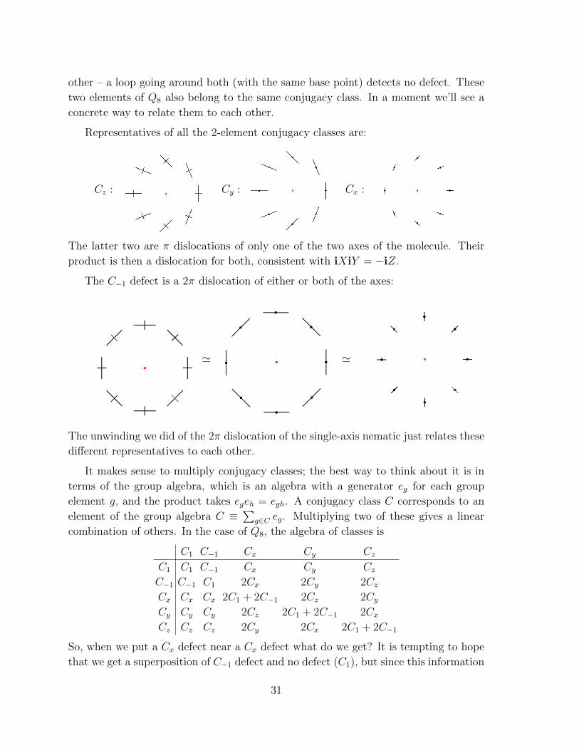
Representatives of all the 2-element conjugacy classes are:
Cz : Cy : Cx :
The latter two are π dislocations of only one of the two axes of the molecule. Their
product is then a dislocation for both, consistent with iXiY = −iZ.
The C−1 defect is a 2π dislocation of either or both of the axes:
' '
The unwinding we did of the 2π dislocation of the single-axis nematic just relates these
different representatives to each other.
It makes sense to multiply conjugacy classes; the best way to think about it is in
terms of the group algebra, which is an algebra with a generator eg for each group
element g, and the product takes egeh = egh. A conjugacy class C corresponds to an
element of the group algebra C ≡∑
g∈C eg. Multiplying two of these gives a linear
combination of others. In the case of Q8, the algebra of classes is
C1 C−1 Cx Cy CzC1 C1 C−1 Cx Cy CzC−1 C−1 C1 2Cx 2Cy 2CzCx Cx Cx 2C1 + 2C−1 2Cz 2CyCy Cy Cy 2Cz 2C1 + 2C−1 2CxCz Cz Cz 2Cy 2Cx 2C1 + 2C−1
So, when we put a Cx defect near a Cx defect what do we get? It is tempting to hope
that we get a superposition of C−1 defect and no defect (C1), but since this information
31
is not too hard to measure I don’t think this is the answer. The answer seems to be
that it depends on the route by which we combine them.
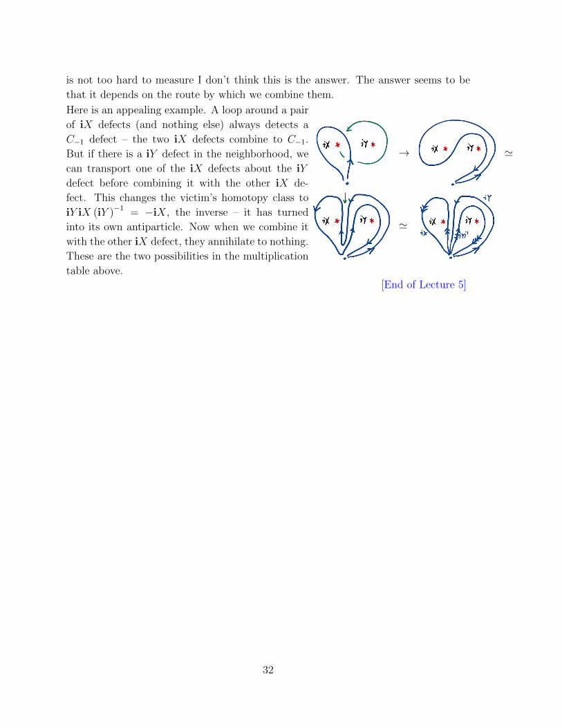
Here is an appealing example. A loop around a pair
of iX defects (and nothing else) always detects a
C−1 defect – the two iX defects combine to C−1.
But if there is a iY defect in the neighborhood, we
can transport one of the iX defects about the iY
defect before combining it with the other iX de-
fect. This changes the victim’s homotopy class to
iY iX (iY )−1 = −iX, the inverse – it has turned
into its own antiparticle. Now when we combine it
with the other iX defect, they annihilate to nothing.
These are the two possibilities in the multiplication
table above.
→ '
'
[End of Lecture 5]
32

1.7 Textures or solitons
In d spatial dimensions, consider now a smooth configuration (no defects) of φ : Rd →V . Let’s demand that the configuration has finite FLG[φ]. In particular, this requires
that φ approach a constant at infinity, φx→∞→ φ0. In this case, φ defines a map Sd → V ,
since Rd plus the point at infinity is Sd. Therefore [φ] ∈ πd(V ). Two such maps φ1,2
can be continuously deformed into each other if and only if [φ1] = [φ2] ∈ πd(V ).
Such smooth but topologically nontrivial configurations are like codimension d+ 1
defects. They are called textures or solitons or skyrmions. The latter name applies in
particular to the cases d = 3, V = G, a simple Lie group, or d = 2, V = S2, as for a
layer of Heisenberg spins. For example in d = 3 with V = SU(2), a nice representative
is of the form eif(r)x·~σ.
Skyrmions are a common sight in various magnetic materials. There are even phases
of matter described by lattices of skyrmions. They also arise in high-energy physics as
a description of baryons in terms of the theory of goldstone bosons for the breaking
of chiral symmetry, the chiral Lagrangian. This was Skyrme’s original, very prescient,
motivation.
Energetic questions. If we do ask about solving the equations of motion, the
story has the following wrinkle. A nonsingular configuration that approaches φ0 at
infinity can be deformed to one that approaches φ0 more quickly by the homotopy
φλ(x) = φ(x/λ), λ < 1. As λ→ 0, the region where φ varies (the soliton) shrinks, and
at λ = 0 a singularity forms. To decide which value of λ is best, we must ask about
the energy of such a configuration. Looking at just the essential leading generalized
rigidity term, we have
F 0LG[φλ] ≡ ρ
∫ddx (∂xφλ)
2 x≡x/λ= ρ
∫ddxλd (∂xφ)2 λ−2 = λd−2FLG[φ].
This goes to zero as λ→ 0. So in d > 2 spatial dimensions, the soliton wants to shrink,
according to the leading term in the effective action. This is called Derrick’s theorem.
As λ shrinks, the gradients of φ get larger. The argument breaks down once the
soliton gets small enough that the terms with more derivatives in FLG start to become
large. By dimensional analysis, such terms must come with a microscopic scale Λ.
For example, the subleading term in the derivative expansion (it depends on what
symmetries we assume) could be 1Λ∆
∫ddx (∂φ)4, with ∆ determined by dimensional
analysis. Under the rescaling φ(x) → φ(x/λ), this term gets a factor of λd−4, which
blows up as λ → 0 for d < 4. This means that FLG[φλ] must have a minimum as a
function of λ – the soliton is stabilized at some size determined by the microscopic
scale Λ.
33

1.8 Defects of broken spatial symmetries
[In preparing this section I found very useful this new paper and this talk by Dominic
Else.]
Here is one idea of why spatial symmetries are more subtle: for internal symmetries,
each broken generator of a continuous symmetry produces an independent goldstone
mode. This is not always the case for spatial symmetries. For example, a crystalline
solid breaks both translations and rotations, but in d space dimensions produces only
d phonon polarizations.
The reason is: a rotation is a position-dependent translation.
Therefore the goldstone mode for rotations is described by a
particular profile of the translation goldstone.
Elasticity theory in terms of goldstones. Let’s pursue this example a bit
further. Suppose a collection of atoms spontaneously forms a crystal – an arrangement
of the atoms into a unit cell which then tiles space according to some lattice. This
breaks continuous translations down to discrete translations by a lattice vector, and so
we expect a goldstone field for each direction of space. I will studiously ignore rotation
symmetries for a little while. Consider for a moment the case of one dimension (and
don’t worry about Hohenberg-Mermin-Wagner issues right now). The symmetry of
the ordered phase is G = R, continuous translations, and the stabilizer group of a
configuration is H = Z, lattice translations, so V = R/Z = S1. The goldstone field
lives on a circle. Shifting the goldstone field by its period shifts each atom by one unit
cell. More generally, V = Rd/Γ = T d where Γ is the lattice. In terms of θI , periodic
coordinates on this torus, the LG free energy is
S[θI ] =
∫dd+1x κijKL∂iθ
K∂jθL + terms with more derivatives, (1.15)
where the coupling constant κijKL is the elasticity tensor. With various symmetries
imposed, it can be decomposed further into various tensors with names from the 19th
century. These tensors describe things like bending moduli – the rigidity of the solid
to various kinds of strain.
For quasicrystals, a similar story obtains. A quasicrystal is a quasiperiodic soild.
That means that the plane is tiled with more than one unit cell in a manner which does
not repeat precisely. The simple way to obtain such a thing is by projecting a D > d-
dimensional lattice with incommensurate periods into d dimensions. This produces a
34

diffraction pattern with D peaks. In this case, the order parameter field lives in TD,
and we can write an effective action just like (1.15) with the only difference that the
K,L indices on the θ variables run from 1..D instead. The extra goldstone modes are
called phasons.
Dislocations. Now let’s talk about defects. You can see that π1(V ) = π1(Rd/Γ) =
Γ, the lattice itself, since Rd is simply connected.
Therefore we can identify the topological charge of a codimension-two lattice defect
– a dislocation – with an element of the lattice. This is called its Burgers’ vector.
Comparing with our prior discussion of vortices, we can say that dislocations are the
vortices of the goldstone field. This comparison allows us to be more quantitative about
the Burgers’ vector: it is given by
bI =1
2π
∮C
dxi∂xiθI =
1
2π
∮θ(C)
dθI
where C is a curve in space going around the dislocation. A dislocation in a 2d square
lattice looks like this:
The usual definition of the Burgers’ vector is shown at right: make a circuit around the
(line) defect, and compare with the corresponding circuit in the perfect lattice. The
Burgers’ vector is the extra stuff you have to add to make it a closed cycle. Here we
go 3 steps up, 3 steps right, 3 steps down, 4 steps left, so the Burgers’ vector is 1 step
right. Notice that you would get the same answer no matter which closed path you
took, winding once clockwise around the defect.
A first encounter with Lieb-Schulz-Mattis-Oshikawa-Hastings constraints.
Suppose the atom number is conserved. (This is not a crazy idea.) Then the system
has another symmetry in addition to translation symmetry, and this symmetry is un-
broken by the crystal, so V is unchanged. This extra symmetry is not necessarily
useless, however. In particular, we can consider coupling to a background gauge field
Aµ for this symmetry. This is a strategy we will employ all the time this quarter so we
35

may as well get started now. I emphasize that Aµ is a fixed background configuration
that we get to pick.
The idea is to follow as before the LG procedure of writing the effective action
by the effective strategy of “what else could it be?” – we write all terms allowed by
symmetries, arranged in order of decreasing relevance to the low-energy physics. In
the presence of a background gauge field, we have a new ingredient, in addition to the
goldstone fields and their derivatives, namely A and its derivatives. But there is also
a new constraint: when we couple a system to a background gauge field, we do it in a
way that is gauge invariant, that is, it is invariant under the gauge transformation
Aµ → Aµ + g−1∂µg (1.16)
for an arbitrary map g : space → U(1) (combined with some rotations of whatever
charged matter fields are involved). So the effective action must also be gauge invariant,
since it arises as the LHS of the equation
eiS[θ,A] =
∫[Dstuff]eiSmicroscopic[stuff,θ,A].
Furthermore, if all excitations besides the goldstones are gapped, then the effective
action S[θ, A] must be local, a single integral over spacetime.
So, what can the effective action be? Note that the goldstones themselves are
neutral under the gauge transformation. Certainly terms involving F = dA are allowed
since F is gauge invariant. But there is one interesting new term which involves the
fewest derivatives, and expresses some important truths for us. To understand it most
immediately, let’s consider the case of d = 1. Then
S[slowly-varying θ, Aµ] = Selastic[θ] +ν
2π
∫A ∧ dθ + terms with more derivatives.
The new term can also be written as
Sν [θ, A] ≡ ν
2π
∫A ∧ dθ =
ν
2π
∫dxdtAµ∂νθε
µν . (1.17)
One point to notice about it is that it is not obviously gauge invariant because it
depends on A and not just F . Under a gauge transformation (1.16), it changes by
δSν =ν
2π
∫dθ ∧ g−1dg. (1.18)
This is not obviously zero. But we don’t actually need the variation of the action to
be zero, we just need it to be an integer multiple of 2πi, since it only ever appears
exponentiated in the path integral. And in fact, if θ and g are continuous functions
36

and spacetime has no boundaries, (1.18) is always 2πiν times an integer. (To see this,
first show that it is invariant under small changes of g or θ:
δ (δSν)
δg=δ (δSν)
δθ= 0.
So it is topological. Then we can compute it for some representative configuration. If,
for definiteness, we periodically identify the spacetime coordinates, (1.18) is an expres-
sion for (2πi times) the winding number of the map T 2 → T 2, (x, t)→ (g(x, t), θ(x, t)).
Note that maps g : spacetime→ G that are not continuously connected to the map to
the identity are called ‘large gauge transformations’.) Therefore, if ν ∈ Z, then (1.17)
is gauge invariant13
What does the new term (1.17) do? Well, the first question we should ask about an
effective action for a background gauge field is: what is the resulting charge density:
ρ(x) =δS
δA0(x)=
ν
2π∂xθ + · · · .
This equation correctly expresses the fact that deforming the lattice away from a uni-
form configuration will make the density vary. The · · · is contributions from other
terms in the action, such as a term like∫A0ρ0 that adds a background density. If
ρ0 is constant in time and integrates to an integer, this is also gauge invariant. More
generally, we could add∫Aµj
µ which you can show is gauge invariant (even under
large gauge transformations) as long as ∂µjµ = 0.
Actually we can do a bit better, and include the ρ0 term in Sν . We can identify the
goldstone field θ with the phase field describing the displacements of the atoms from
their equilibrium positions:
ui(x, t) =1
2πaiIθ
I(x, t)− xi
where ~aI are generators of the lattice Γ. Then the equilibrium configuration is actually
θI(x, t) = KIi x
i where KIi
(a
2π
)jI
= δji , so KIi is the matrix whose columns are the
reciprocal lattice generators. The generalization of (1.17) in d spatial dimensions is
ν
(2π)d
∫A ∧ dθ1 ∧ dθ2 · · · ∧ dθd . (1.19)
13Alternatively, if spacetime is a manifold without boundary, we can integrate by parts and write
Sν = − ν
2π
∫θ ∧ F.
This is manifestly gauge invariant, but it is not manifestly single-valued under θ → θ+ 2π, as it must
be to be well-defined. Fortunately,∫SF/2π ∈ Z is an integer if A is a background U(1) gauge field on
a manifold S without boundary (this is called flux quantization), and so again we conclude that eiSν
is well-defined if ν ∈ Z.
37

Again ν ∈ Z is required by gauge invariance. This gives the density
ρ(x) =δS
δA0(x)=
ν
(2π)d1
d!εI1···Idε
i1···id∂xi1θI1 · · · ∂xidθ
Id .
Plugging in the equilibrium configuration gives
ρ0(x) = νdetK
(2π)d=ν
V
where V ≡ det a is the volume of the unit cell. This says that ν is the (integer!)
number of atoms per unit cell. [End of Lecture 6]
By the gauge invariance argument above, under the present assumptions, ν, and
hence the equilibrium density must be an integer. This is an avatar of the Lieb-
Schulz-Mattis-Oshikawa-Hastings (LSMOH) theorem, which will be our companion
this quarter. Now, you may say to yourself, why can’t I make a system at some filling
which is not an integer? Indeed, I can take 20007 particles and place them in a volume
with 20004 unit cells, and the system must have some groundstate. What gives? Well,
there are two loopholes in our argument, both at the ‘what else can it be?’ step.
1. One we made explicit: if the system has gapless degrees of freedom in addition to
the phonons, then the effective action for just the goldstones and the background
gauge field need not be local – integrating out gapless stuff produces a nonlocal
action.
One specific way in which the system can be gapless is if it spontaneously breaks
the U(1) atom number symmetry. Then there is an additional goldstone that we
haven’t included in our description.
2. The other possibility is that the system does not have a unique groundstate, but k
of them; in that case ν may be a multiple of 1/k. The large gauge transformations
can then take one of these groundstates to another.
This can also arise in two ways: if the system preserves all the symmetries, this is
topological order. But degenerate groundstates can also arise from spontaneously
breaking the lattice translation symmetry further to a discrete subgroup. Such a
thing is called a charge density wave.
The statement of the theorem then is: if the filling is not an integer, the system
(ignoring the phonons) must be interesting – it must be gapless or have degenerate
groundstates. Notice that this result arises from some interesting interplay between
translation symmetry and the internal U(1) symmetry associated with particle number
conservation.
38

I should be more explicit about the second, more subtle possibility. In the discus-
sion above I always mean the groundstate in the presence of the background fields. It?s
important that the groundstate responds (adiabatically) to the background fields. The
basic idea of why groundstate degeneracy allows the effective action S[A] to be not
single-valued is spectral flow. I will say a lot more about this. A large gauge transfor-
mation is a gauge transformation not continuously connected to the identity element.
A good example of a large gauge transformation to keep in mind is threading 2π flux
through a cylinder. But think of this as the endpoint of a path where we gradually
increase the amount of flux. At intermediate stages of the cycle, the energy levels move
around. We start in some groundstate. If there is not a unique groundstate, the final
groundstate need not be the same one.
Flux-threading. Actually, this is a good opportunity to introduce a technique we
will use repeatedly below. Consider ν = 12
– one particle for every other lattice site.
How can we make a state with a gap (at fixed θ)? One way to do it is just to break
translation invariance Z → 2Z, i.e. double the unit cell. For example, put a particle
in every other site. However we do it, there are inevitably two such states related by
a translation by one lattice site, which I’ll denote by |•〉 and |•〉. It will be useful to
make eigenstates of the lattice momentum (defined modulo 2π in units of one over the
lattice spacing):
|P = 0〉 = |•〉+ |•〉 , |P = π〉 = |•〉 − |•〉 . (1.20)
Now put the system on a big circle with an even number of lattice sites L ∈ 2Z, so
that our pattern fits. The idea is, as I said above, that a large gauge transformation is
the endpoint of a path of configurations of the background gauge field A. Φ ≡∮A =∫ L
0Axdx is the flux of the background gauge field through the circle. Since charge is
quantized, 2π flux is the same as no flux. Another way to look at it is that gauge
transformation relates
A→ A+ ig−1dg (1.21)
and if g = gn ≡ e−2πinx/L, we have Φ→ Φ +∮
ig−1n dgn = Φ + 2πn.
So let’s choose a path in the space of gauge fields from Φ = 0 to Φ = 2π:
A(t) =2π
Lf(t)dx, f(0) = 0, f(T ) = 1. (1.22)
so Φ(t) =∮A =
∫ L0dx2π
Lf(t) = 2πf(t). If we start the system in a groundstate and do
this process slowly enough (T−1 the gap to non-phonon excitations) – with a fixed
39

configuration of the phonons θ – we must end up in a groundstate. This is because14
∂E
∂Φ= 〈I〉
the average current, which must vanish for a gapped system, in the thermodynamic
limit. So the energy ends up at the same value as it started.
Now use Newton’s laws. The gauge field configuration in (1.22) implies an electric
field in the x direction
Ex =∂Ax∂t
=2π
Lf ′(t) (1.23)
which exerts a force on each particle. The total change in (lattice) momentum of the
system is then
∆P =
∫ T
0
dt∑i
Ex(i) = N2π
L
∫ T
0
f ′(t)dt =2πN
L= 2πν
where N is the number of particles.
We conclude that this flux-threading process, done at ν = 12
must interchange
|P = 0〉 and |P = π〉15 But the result of this process is the image under the large gauge
transformation g1. We conclude that only gn with n a multiple of 1/ν takes a given
groundstate to itself, and Sν is a perfectly-allowed term in the action.
I emphasize that the conclusion that threading π-flux takes one groundstate to an-
other that must be orthogonal (because it has a different eigenvalue of a hermitian
operator, namely the momentum) holds even if translation symmetry is not sponta-
neously broken.
14This is basically the same statement as δSδA = j. The extra ingredient is that the phase acquired
by a state evolving for time T of a state with energy E is ET .15perhaps with a phase that we haven’t determined by this argument. If there is no phase, we could
conclude that flux-threading acts in the basis |•〉 , |•〉 as σx. Can that be right?
40

Mobility constraints on dislocations. The preceding discussion also tells us
something about the ability of dislocations to move. Let’s focus on the case d = 2
since it is drawable (and the dislocations are codimension two anyway). The claim is
that if ν 6= 0, then a dislocation can only move in the direction of its Burgers’ vector.
First let’s see this by pictures:
We see that in order to move transverse to the Burgers’ vector, an atom (the red one
in the top right figure) must be created from nothing (or ferried in from ∞ by moving
a whole line of atoms by one lattice vector).
Earlier we considered only the atom number density by varying the effective action.
The full atom number current in 2d is
jµ =δS[θ, A]
δAµ(x, t)=
ν
8π2εµνρ∂νθ
I∂ρθJεIJ .
The usual (totally correct) story is that gauge invariance guarantees current conserva-
tion. Our effective action with the interesting term Sν is indeed gauge invariant for
41
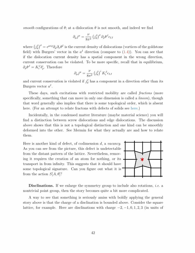
smooth configurations of θ; at a dislocation θ is not smooth, and indeed we find
∂µjµ =
ν
8π2
(jId)ρ∂ρθ
JεIJ
where(jId)ρ
= εµνρ∂µ∂νθI is the current density of dislocations (vortices of the goldstone
field) with Burgers’ vector in the aI direction (compare to (1.4)). You can see that
if the dislocation current density has a spatial component in the wrong direction,
current conservation can be violated. To be more specific, recall that in equilibrium,
∂ρθJ = KJ
i δiρ. Therefore
∂µjµ =
ν
8π2
(jId)iKJi εIJ
and current conservation is violated if jId has a component in a direction other than its
Burgers vector aI .
These days, such excitations with restricted mobility are called fractons (more
specifically, something that can move in only one dimension is called a lineon), though
that word generally also implies that there is some topological order, which is absent
here. (For an attempt to relate fractons with defects of solids see here.)
Incidentally, in the condensed matter literature (maybe material science) you will
find a distinction between screw dislocations and edge dislocations. The discussion
above shows that this is not a topological distinction and one kind can be smoothly
deformed into the other. See Mermin for what they actually are and how to relate
them.
Here is another kind of defect, of codimension d, a vacancy.
As you can see from the picture, this defect is undetectable
from the distant pattern of the lattice. Nevertheless, remov-
ing it requires the creation of an atom for nothing, or its
transport in from infinity. This suggests that it should have
some topological signature. Can you figure out what it is
from the action S[A, θ]?
Disclinations. If we enlarge the symmetry group to include also rotations, i.e. a
nontrivial point group, then the story becomes quite a bit more complicated.
A way to see that something is seriously amiss with boldly applying the general
story above is that the charge of a disclination is bounded above. Consider the square
lattice, for example. Here are disclinations with charge −2,−1, 0, 1, 2, 3 (in units of
42

π/2), respectively.
· · ·
The charge is the deficit angle, in units of π/2 for convenience. (More precisely, by
deficit angle I mean the difference between 2π and the angle one would turn by in going
in a loop around the defect if each turn were actually π/2, as it is on the perfect lattice.
When the angle is negative, it is hard to draw this way on the plane; we could have
drawn it as a branched cover of the plane.) A disclination of charge 4 on the square
lattice is no lattice at all! But the charge can become arbitrarily negative.
Trying nevertheless, we would say that a general defect of a lattice is labelled by a
conjugacy class of
π1(V ) = π1
(translations n rotations
Γ n point group, K
)= Γ n K
where K is the cover of the point group that lifts it to a subgroup of the universal
cover of the rotation group (I think it’s called the ‘double group’). π1(V ) is generally
a complicated non-abelian group. An interesting consequence of its non-abelianness is
that two disclinations can have the same topological charge as a dislocation.
To avoid too much crystallography (not my favorite part of condensed matter
physics), let’s just talk about the square lattice. For the square lattice,
π1(V ) = Z2 n 〈R ≡ π/2 rotation〉 = (~a,Rk).
The group law is
(~a,Rk)(~a′, Rk′) = (~a+Rk~a′, Rk+k′).
What are the conjugacy classes? Well, the inverse is
(~a,Rk)−1 = (−R−k~a,R−k).
The conjugacy class of an elementary π/2 dislocation (~0, R) contains all the elements
(~a,Rk)(~0, R)(~a,Rk)−1 = (~a−R~a,R).
This means that
(~0, R) ' ((1, 1), R) ' ((1,−1), R) ' ((n,m), R),∀ n+m even.
43

This means a collection of two disclinations (~0, R) and (~0, R−1) have the same charge
as any dislocation the components of whose Burgers’ vector sum to an even number.
Here are some picture (from Mermin):
You can see that as the distance between the two disclinations grows, so does the
magnitude of the resulting Burgers’ vector ((1, 1), (2, 2), (3, 3) respectively). But these
are all in the same conjugacy class.
An isolated disclination is not mobile at all (even without atom conservation)–
its motion requires the rearrangement of infinitely many atoms. However, we’ve just
seen that a pair of opposite-charge dislocations describes a dislocation, and can move
together in the direction perpendicular to their separation (the Burgers’ vector of the
dislocation). A coarse summary is this phenomenon is the statement that in addition to
the charge of a disclination being a (topological) conserved quantity, the dipole moment
of disclination charge is also conserved. For more on this description, I recommend
again this paper about fractons and elasticity.
1.9 The boojum and relative homotopy
I promised one more application of relative homotopy. Recall that in the A phase of 3He,
the linearly-transforming order-parameter field is of the form Aiα = dα(e(1) + ie(2)
)i,
and e(1), e(2), ˆ ≡ e(1) × e(2) form an orthonormal frame that completely breaks the
rotation symmetry. The order parameter space is
VA =(S2 × SO(3)
)/Z2.
Now put this medium in a space with boundary, i.e. put the helium in a container.
A boundary condition that actually occurs in practice is that the vector ˆ is fixed to
point normal to the wall of the container. Since ˆ is fixed, only the rotations in the
44
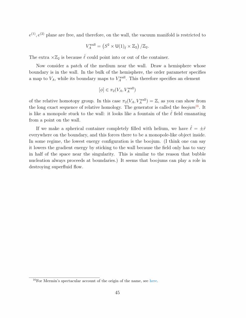
e(1), e(2) plane are free, and therefore, on the wall, the vacuum manifold is restricted to
V wallA =
(S2 × U(1)ˆ× Z2
)/Z2.
The extra ×Z2 is because ˆ could point into or out of the container.
Now consider a patch of the medium near the wall. Draw a hemisphere whose
boundary is in the wall. In the bulk of the hemisphere, the order parameter specifies
a map to VA, while its boundary maps to V wallA . This therefore specifies an element
[φ] ∈ π2(VA, VwallA )
of the relative homotopy group. In this case π2(VA, VwallA ) = Z, as you can show from
the long exact sequence of relative homology. The generator is called the boojum16. It
is like a monopole stuck to the wall: it looks like a fountain of the ˆ field emanating
from a point on the wall.
If we make a spherical container completely filled with helium, we have ˆ = ±reverywhere on the boundary, and this forces there to be a monopole-like object inside.
In some regime, the lowest energy configuration is the boojum. (I think one can say
it lowers the gradient energy by sticking to the wall because the field only has to vary
in half of the space near the singularity. This is similar to the reason that bubble
nucleation always proceeds at boundaries.) It seems that boojums can play a role in
destroying superfluid flow.
16For Mermin’s spectacular account of the origin of the name, see here.
45

2 Some quantum Hall physics
By popular request, and because it still provides the best experimental examples of all
the most interesting quantum topology phenomena, let’s spend some time talking about
effective descriptions of quantum Hall physics, both fractional and integer. I warn you
that we will take a distinctly macroscopic perspective, and, like in our discussion of
topological defects, will not say much about the important microscopic questions of
energetic competition. For a perspective on those questions, I recommend chapters
12-14 of the textbook by Girvin and Yang (or these lectures by Leggett). I learned
about this aspect of the subject from these notes by Girvin. For a great account of the
whole subject I recommend David Tong’s lectures.
Topological states of quantum matter. There are two main ways in which a
state of matter can be topological: protected edge states and topological order. Frac-
tional quantum Hall systems exhibit both of these phenomena, while integer quantum
Hall states only exhibit the former.
Topological order means a robust spacetime-topology-dependent groundstate de-
generacy. Associated with this phenomenon is also a fractionalization of the quantum
numbers of the microscopic constituents. That is, the emergent quasiparticle excita-
tions carry quantum numbers (statistics, spin, charge) which are rational fractions of
those of the constituents. Particles of fractional spin are called anyons. In three space
dimensions, there are also string excitations with robust and interesting fractional
properties.
These two symptoms of topological order are not independent. The fractional
statistics of the quasiparticles implies a groundstate degeneracy on e.g. the torus: Pair-
create a quasiparticle-antiquasiparticle pair, move them around a spatial cycle, and
then re-annihilate them. This process Fx maps one groundstate to another. But Fxdoes not commute with Fy, by the anyonic statistics. The space of groundstates must
represent the algebra of these operators. Conversely, a robust groundstate degeneracy
requires that the different groundstates are related by the action of non-local operators.
In cases where the groundstate degeneracy is independent of geometry17, these non-
local operators describe the transport of fractionalized excitations around the cycles of
the space. [End of Lecture 7]
A third essential symptom of topological order is long-range entanglement in the
groundstate wavefunction. The groundstate cannot be made from a product state by a
17In contrast, in type-2 fracton models, the operators taking one topological groundstate to another
are supported on fractals, and so are hard to interpret as transporting anyons. In such models the
groundstate degeneracy depends (in a complicated way) on the system size, and not just on the
topology.
46

finite-depth local unitary circuit. Actually there are some exceptional states with this
property but which nevertheless do not have topological order, namely integer quantum
Hall states and a few other examples we’ll discuss below. A sharper diagnostic is the
topological entanglement entropy, defined in terms of the entanglement entropy of a
subsystem, which vanishes if and only if there are no anyons.
Let’s enshrine these symptoms of topological order in a list:
1. Fractionalization of quantum numbers.
2. Groundstate degeneracy that depends on the topology of space.
3. Long-ranged entanglement.
I emphasize that the quantum numbers (their statistics and (if there are global
symmetries) charges) characterize the phase of matter. Especially in D = 2 + 1, the
theory of anyons (their statistics and fusion rules) is a highly-developed mathematical
edifice, called unitary modular tensor category (UMTC) theory. Perhaps now is a good
time to mention the most elementary distinction, between abelian and non-abelian
topological order. By fusion of anyons, I mean the following. An anyon is a particle
whose presence can be detected from a distance, by circling some other excitation
around it and measuring the change of the resulting state. Given two anyon types
a and b, I can consider circling other excitations around both of them. If I have a
complete basis of all the anyon types in the topological order under study, the result
must look like one of them, but which one we get need not be uniquely determined:
a× b = c1 + c2 + · · · . (2.1)
If the fusion rules look like
a× b = c
for all the anyons, we say the topological order is abelian. Braiding such particles
merely acts by a phase on the resulting unique state. In contrast, fusion rules like (2.1)
require that the lowest-energy state in the presence of a and b is degenerate; in this
case, braiding the two particles involves not only a phase, but a whole unitary matrix
acting on this degenerate subspace.
If you have studied conformal field theory (CFT), you will notice a formal similarity
between (2.1) and the operator product expansion. This is not a coincidence – a 2d
CFT also defines a UMTC. In fact, the structure was defined first in that context, by
Moore and Seiberg.
47

2.1 Electromagnetic response of gapped states in D = 2 + 1
Let’s think about a gapped state of matter made of some stuff in D = 2 + 1, out of
which we can construct a conserved U(1) current jµ (if you like, think of it as electron
number). This means we can couple this current to an external, background, non-
dynamical gauge field Aµ, by adding to the action functional like so:
Smicroscopic[the stuff,A] = Smicroscopic[the stuff] +
∫jµAµ + · · ·
where · · · is whatever other terms are need to make this action gauge invariant. Here
we’ll treat A as a background field that we control18. Integrate out the stuff to see the
electromagnetic response:
eiSeff[A] ≡∫
[Dstuff]eiS[stuff,A].
In the previous section, we already used the fact that the term linear in A gives the
current density:
〈jµ(x)〉 =δ
δAµ(x)Seff (2.2)
where the RHS is evaluated on the configuration of background fields of interest, which
could be A = 0. Terms quadratic in A encode linear response:
〈jµ(x)jν(y)〉 =δ2
δAµ(x)δAν(y)Seff.
Recall that 〈jj〉 is the main ingredient in Kubo’s formula for the conductivity.
Because the stuff is gapped, Seff is local. By the Landau-Ginzburg-Wilson logic,
we can then determine Seff[A] in a derivative expansion, as follows. To figure out the
power counting, note that A is a gauge field, which is something that we can add to
a derivative to make it a covariant derivative; therefore A has dimension 1, it counts
the same as a derivative.
Seff[A] =
∫ 0 · A2︸ ︷︷ ︸no symmetry breaking
+ν
4πA ∧ F +
1
g2F··F ··
+ · · · . (2.3)
(F = dA.) The A2 term is forbidden by gauge invariance19. With time-reversal
symmetry (and only one gauge field), ν = 0. If ν 6= 0, Maxwell is less important than
18Notice that what we’ve done here is not gauging the U(1) symmetry. We are not changing the
Hilbert space of the system. The background gauge field here is just like a particular collection of
coupling constants19To make it gauge invariant, we would have to add more (gapless) degrees of freedom, in particular
the Goldstone mode φ for the broken U(1) symmetry, which would appear in the gauge-invariant
combination (∂µφ+Aµ)2.
48

the term with ν, the Chern-Simons (CS) term. (Actually, without Lorentz invariance
we can have non-vacuum dielectric constant and magnetic permittivity ε, µ, but this
won’t affect our story.)
The Kubo formula says that the Hall conductivity is:
σxy = limω→0
1
iω〈jxjy〉︸ ︷︷ ︸
= δδAx(k)
δδAy(k)
Seff[A]
|k=0 =ν
2π
in experimenter’s units= ν
e2
h.
The analogous Kubo formula for the longitudinal conductivity σxx says that it is
zero. This is one sense in which the system is an insulator. Note that one could argue
with this characterization, since ρij = (σ−1)ij has ρxx = 0, like a perfect conductor.
While it’s true that there is no dissipation (since the current is perpendicular to the
voltage drop), no charge moves in the direction of the electric field so I think it’s safe
to call it an insulator. Also, there’s an energy gap (by assumption).
Next we’ll show that, if there is no fractionalization, ν is quantized to be an integer.
So different values of ν are distinct states, since an integer can’t change continuously.
(Note that there could be other distinctions – states with the same ν could be distinct.)
Notice that 2d is special here because the conductivity is essentially dimensionless,
and moreover the resistance is independent of the width of the sample:
Rxy = Vy/Ix = EyWy/Ix = Ey/jx =1
σxy.
(Here Wy is the width of the sample in the y direction, perpendicular to the current,
along the direction of voltage drop.) So it makes sense to say that σxy is quantized (in
units of the quantum of conductivity e2
h).
Flux-threading. I must emphasize that the following argument involves an im-
portant special case of studying the response of the system to background fields, called
flux-threading. Rather than thinking about static background EM fields, we consider
EM fields that slowly vary in time – in a loop.
Consider the system on an annulus (sometimes called, in this
context, the ‘Corbino geometry’). Adiabatically thread 2π
worth of magnetic flux through (a solenoid in) the hole in
the annulus. This means we slowly vary the magnetic field
in the hole, so that the change in flux is the flux quantum
Φ0 ≡ hce
= 2π.
49

In the following equation only I restore un-natural units:
Φ0 = ∆Φ =
∫dt∂t
(∫hole
d~a · ~B)
Faraday= −c
∫dt
∮C
~E · d~ jr=σxyEϕ= − c
σxy
∫dtjr︸ ︷︷ ︸
=∆Q
where C is a curve going around the hole. We conclude that an amount of charge
∆Q =Φ0
cσxy = νe (2.4)
(e is the charge of the electron) is transferred from one edge of the cylinder to the other.
Because of the energy gap, we can do the flux-threading adiabatically. Moreover, the
initial and final Hamiltonians are related by a gauge gransformation:
H(Φ = 0) ∼= H(Φ = 2π).
(We detect a magnetic field by moving a charged particle around a loop and acquiring
a phase eiq∮C A; since the charge is quantized to be an integer, 2π flux is the same as
no flux.) They have the same spectrum. Moreover, the work done on the system is∫IdΦ ∝
∫dt(dΦdt
)2which goes to zero in the thermodynamic limit, if our process is
adiabatic. Therefore the initial and final states must be degenerate in the thermody-
namic limit. But the adiabatic deformation can take one state to another. The states
differ in that an amount of charge ν has been moved from one boundary to the other.
Since, in the absence of fractionalization, charge is carried only by electrons, localized
objects with integer charge, we conclude Z 3 ν = ∆Q/e = σxy.
If we make the further assumption that the states can be labelled with the same
labels as free-electron states, i.e. electron occupation numbers, we can say more. We’ve
identified two different states related by the flux threading. The single-particle states
whose occupation numbers have changed must lie near the Fermi level. Since we’ve
assumed the bulk is gapped, we conclude that there must be gapless edge states.
The following argument implies further that a gapped system with σxy = ν e2
h
hosts a particle excitation with exchange statistics πν.
Now consider the system on the plane. Adiabatically thread 2π worth of localized
magnetic flux through some localized region R of the sample (as in the ⊗ at right).
To do this, we have to stick a really thin solenoid through the 2d surface on which the
system lives. This means as above that (I now return to units with ~ = c = e = 1)
2π = ∆Φ =
∫dt∂t
(∫R|∂R=C
d~a · ~B)
Faraday= −
∫dt
∮C
~E · d~ jr=σxyEϕ= − 1
σxy
∫dtjr︸ ︷︷ ︸
=∆Q
.
50

We conclude that the inserted flux sucks in an amount of charge
∆Q = νe.
Because of the energy gap, we can do this adiabatically. And because the flux is a
multiple of 2π we end up with another state of the same system – the inserted flux is
not an extrinsic defect20. This object is a localized excitation of the system – it can
move around, it’s a particle21. And if ν /∈ Z, it has fractional charge νe.
[End of Lecture 8]
But now consider two of them. From the Bohm-Aharonov effect, each has statistics
angle πσxy (for σxy = e2
h, this is a fermion). Therefore, no topological order (hence no
fractional statistics) implies that σxy ∈ Z e2
h.
This argument has a stronger consequence for bosons: For a system made only of
bosons, without topological order, σxy must be an even multiple of e2
h. For a careful
recent discussion of these arguments, see here.
In a gapped state with no fractionalization, all particles, including this one, must
have the same statistics as the microscopic constituents. For a non-fractionalized state
made from fermions, this means ν ∈ Z. For bosons, no fractionalization implies ν ∈ 2Z.
Roles of topology. Quantum Hall insulators provide examples that are topological
in two distinct ways. The Hall conductivity (apply small electric field in x direction,
measure current in y direction, take ratio)
σxy =p
q
e2
h(2.5)
is a rational number – p, q ∈ Z – despite (in fact, with the help of)22 disorder. The
integer quantum Hall effect (IQHE) is governed by (2.5) with q = 1. It happens for
20This is slightly less obvious than in the case where the flux was in a hole in the system. Put the
solenoid at the origin and choose the gauge A = Φ0dϕ2π , where ϕ is the azimuthal coordinate in the
plane (this is the field involved with the flux-threading, in addition to any magnetic field responsible
for supporting the quantum Hall state). The gauge transformation that removes A is g = eiϕ, which
is singular at the origin of polar coordinates. This singularity has no effect, since it just changes the
overall phase of the wavefunction, Ψ→ Ψ∏j e
iϕj .21Here’s something I’m confused about at the moment. Unlike in the case of the ‘Corbino geometry’
above, where the flux was inserted in a hole in the sample, in this case we do expect that the final
state has a different energy than the initial state – the quasiparticle we’ve created has some rest mass
larger than zero, and (by charge conservation) the gap should be of order twice this value. Where
does the argument about the work done break down?22If the system is translation invariant, one can show that the Hall conductivity must be strictly
linear in the continuously-variable filling fraction ν = ρΦ0/B (ρ is the electron density, Φ0 = hc/e is
the flux quantum), so there can be no quantized plateaux. One possibility for breaking the symmetry
51

free electrons filling Landau levels or Chern bands. The quantization p ∈ Z arises
because of topology of single-particle orbits; p is the Chern number. This does not
exhibit topological order. This is an example of a ‘topological insulator’. It is a band
insulator – the electrons completely fill some bands, and therefore there is an energy
gap, measured by the energy difference to the next band (or to the next Landau level,
i.e. the cyclotron frequency eB/m).
The fractional quantum Hall effect (FQHE) is described by q > 1, requires interac-
tions, topological order. q ∈ Z because of topology of many-body wave function. The
electron fractionalizes: excitations have charge 1/q, fractional statistics.
Perhaps I should pause to emphasize that so far we have assumed that a bunch of
stuff in D = 2 + 1 with a conserved charge but without time-reversal symmetry (such
as a 2d electron gas in a magnetic field) can form a state with an energy gap. What
we’ve shown, using the Landau-Ginzburg-Wilson logic, is that if this does happen, the
system exhibits a quantized Hall conductivity. It is a remarkable fact, not at all obvious
from anything we’ve said here, that this actually happens. As evidence, I include the
classic plot:
In this plot, the electron density is fixed, and the horizontal axis varies B. The key
point is that around the value of B where the actual filling fraction (number of electrons
per flux quantum) hits certain microscopically-preferred rational values, the measured
σxy shows a plateau (along which σxx = 0), in striking contrast with the prediction
from translation symmetry23 When deforming away from the middle of the plateau,
leading to this conclusion is disorder; this is the sense in which it helps. (It is then less obvious that it
doesn’t just make the Hall conductivity zero by Anderson localizing all the states.) Another possibility
is that the symmetry could be broken spontaneously, as discussed here. It seems to me that another
possibility could be boundaries of the sample.23Theorem: translation symmetry implies σxy = ρec
B , where ρ is the electron density. Consider the
52

the extra electrons must somehow be prevented from participating in the transport –
they are somehow localized, either by disorder or by forming a (Wigner) crystal.
2.2 Abelian Chern-Simons theory
[Wen’s book or this review; Zee, Quantum Hall Fluids; Zee’s QFT book §VI.2] I want
to explain an example of how properties 1 and 2 can be realized in a simple physical
system, using the EFT (effective field theory) that describes the canonical examples of
topologically-ordered states: (abelian) fractional quantum Hall states in D = 2 + 1.
The low-energy effective field theory is Chern-Simons-Witten gauge theory, whose
basic action is:
S0[aI ] =n∑IJ
KIJ
4π
∫aI ∧ daJ (2.6)
aI are a collection of abelian gauge fields.
Where did these gauge fields come from? We’ll discuss some perhaps-more-informative
possibilities below, but one very simple way to motivate their introduction is as follows.
By assumption, our system has a conserved U(1) current, Jµ, satisfying ∂µJµ = 0. In
D = 2 + 1, we can solve this equation by introducing a field a and writing
Jµ = εµνρ∂νaρ. (2.7)
The continuity equation is automatic if J can be written this way (for nonsingular a) by
symmetry of the mixed partials. (The equation could also be solved by a sum of such
terms, as we write below. This ambiguity reflects some of the enormous multiplicity
of different quantum Hall states.) Then we must guess what dynamics should govern
a. Here we just add all terms allowed by the symmetries, as usual. When it’s not
Hamiltonian H for a 2d collection of electrons in a uniform magnetic field ~B = Bz, with ~E = Ey
uniform as well. Choose the gauge ~A(r, t) = (−cEt + Bx)y. Gauge invariance means that the
momentum of the ith electron appears in H only in the combination ~Π = ~pi + ec~A(ri, t). Remove the
Et term by changing variables to ~r′i = ri − cEB tx, ~p′i = pi, t
′ = t. The current in the new frame is j′x =
−ρe⟨X ′⟩
where X ′ is the center-of-mass position in the x direction. The center-of-mass momentum
in the y direction P ′y = Py ≡∑j(pj)y is conserved. Therefore if
⟨X ′⟩6= 0, Π′y =
∑i((p
′i)y + e
cBX′
would blow up. We conclude that 0 =⟨X ′⟩∝ j′x = 0. But ~J ′(r′) = ~J(r) + ecEBρx and therefore
Jx = −ρecEB
= σxyEy
from which we conclude σxy = ρecB without any further assumptions. A closely-related argument
assuming boost invariance appears in many places, in particular in the Girvin lectures.
53
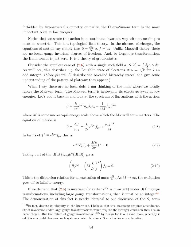
forbidden by time-reversal symmetry or parity, the Chern-Simons term is the most
important term at low energies.
Notice that we wrote this action in a coordinate-invariant way without needing to
mention a metric. This is a topological field theory. In the absence of charges, the
equations of motion say simply that 0 = δS0
δa∝ f = da. Unlike Maxwell theory, there
are no local, gauge invariant degrees of freedom. And, by Legendre transformation,
the Hamiltonian is just zero. It is a theory of groundstates.
Consider the simplest case of (2.6) with a single such field a, S0[a] =∫
k4πa ∧ da.
As we’ll see, this describes e.g. the Laughlin state of electrons at ν = 1/k for k an
odd integer. (More general K describe the so-called hierarchy states, and give some
understanding of the pattern of plateaux that appear.)
When I say there are no local dofs, I am thinking of the limit where we totally
ignore the Maxwell term. The Maxwell term is irrelevant: its effects go away at low
energies. Let’s add it back in and look at the spectrum of fluctuations with the action:
L =k
4πεµνρaµ∂νaρ +
1
4Mfµνf
µν
where M is some microscopic energy scale above which the Maxwell term matters. The
equation of motion is
0 =δS
δaλ=
k
2πελρνfρν +
∂µfµλ
M. (2.8)
In terms of fλ ≡ ελρσfρσ this is
εµνρ∂νfρ +Mk
2πfµ = 0. (2.9)
Taking curl of the BHS (εµαβ∂α(BHS)) gives(∂µ∂
µ −(M
k
2π
)2)fρ = 0. (2.10)
This is the dispersion relation for an excitation of mass Mk2π
. As M →∞, the excitation
goes off to infinite energy.
If we demand that (2.6) is invariant (or rather eiS0 is invariant) under U(1)n gauge
transformations, including large gauge transformations, then k must be an integer24.
The demonstration of this fact is nearly identical to our discussion of the Sν term
24In fact, despite its ubiquity in the literature, I believe that this statement requires amendment.
Strict invariance under large gauge transformations would require the stronger condition that k is an
even integer. But the failure of gauge invariance of eiS0 by a sign for k = 1 (and more generally k
odd) is acceptable because such systems contain fermions. See below for an explanation.
54
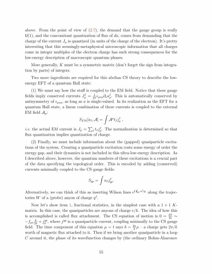
above. From the point of view of (2.7), the demand that the gauge group is really
U(1), and the concomitant quantization of flux of da, comes from demanding that the
charge of the current Jµ is quantized (in units of the charge of the electron). It’s pretty
interesting that this seemingly-metaphysical microscopic information that all charges
come in integer multiples of the electron charge has such strong consequences for the
low-energy description of macroscopic quantum phases.
More generally, K must be a symmetric matrix (don’t forget the sign from integra-
tion by parts) of integers.
Two more ingredients are required for this abelian CS theory to describe the low-
energy EFT of a quantum Hall state:
(1) We must say how the stuff is coupled to the EM field. Notice that these gauge
fields imply conserved currents J Iµ = 12πεµνρ∂νa
Iρ. This is automatically conserved by
antisymmetry of εµνρ, as long as a is single-valued. In its realization as the EFT for a
quantum Hall state, a linear combination of these currents is coupled to the external
EM field Aµ:
SEM [aI ,A] =
∫AµtIjIµ ,
i.e. the actual EM current is Jµ =∑
I tIjIµ. The normalization is determined so that
flux quantization implies quantization of charge.
(2) Finally, we must include information about the (gapped) quasiparticle excita-
tions of the system. Creating a quasiparticle excitation costs some energy of order the
energy gap, and their dynamics is not included in this ultra-low-energy description. As
I described above, however, the quantum numbers of these excitations is a crucial part
of the data specifying the topological order. This is encoded by adding (conserved)
currents minimally coupled to the CS gauge fields:
Sqp =
∫aIj
Iqp.
Alternatively, we can think of this as inserting Wilson lines ei∮W aIqI along the trajec-
tories W of a (probe) anyon of charge qI .
Now let’s show item 1, fractional statistics, in the simplest case with a 1 × 1 K-
matrix. In this case, the quasiparticles are anyons of charge e/k. The idea of how this
is accomplished is called flux attachment. The CS equation of motion is 0 = δSδa∼
−fµν k2π
+ jqpµ , where jqp is a quasiparticle current, coupling minimally to the CS gauge
field. The time component of this equation µ = t says b = 2πkρ – a charge gets 2π/k
worth of magnetic flux attached to it. Then if we bring another quasiparticle in a loop
C around it, the phase of its wavefunction changes by (the ordinary Bohm-Aharonov
55

effect)
∆ϕ12 = q1
∮C
a = q1
∫R,∂R=C
b = q12π
kq2.
Hence, the quasiparticles have fractional braiding statistics25 .
Now topological order property 2: # of groundstates = |det(K)|genus. Consider
the simplest case, where K = k, and put the system on a torus T 2 = S1 × S1. The
gauge-invariant operators acting on the Hilbert space of the CS theory on a torus are
of the form Fx ≡ ei∮Cx
a,Fy ≡ ei∮Cy
aand integer powers of these operators. These
are the operators that transport the anyons around the cycles of the torus. The re-
striction to integers comes from the demand that they are invariant under large gauge
transformations, which take∮Ca→
∮Ca+ 2πZ. According to the CS action, ax is the
canonical momentum of ay. Canonical quantization then implies that
[ax(r), ay(r′)] =
2πi
kδ2(r − r′)
and hence (by the BCH formula) that these flux-insertion operators satisfy a Heisenberg
algebra: FxFy = FyFxe2πi/k. The smallest irrep of this algebra is k dimensional, where
Fx and Fy look like clock and shift matrices.
[End of Lecture 9]
If space is a Riemann surface with g handles (like this: ),
then there are g pairs of such operators, so g independent Heisenberg algebras, all of
which commute with the Hamiltonian, and hence kg groundstates.
It is also possible to show that CS theory also exhibits the third property of long-
range entanglement. See here.
This description shows a quasiparticle with charge e/k: If we stick in a quasiparticle
at the origin, the equations of motion become
0 =δS
δa0(x)=
k
2πfxy − δ2(x). (2.11)
From the relation Jµ = e2πεµνρ∂νaρ, the actual electric charge is then
ρ = e1
2πfxy =
e
kδ2(x). (2.12)
25The fractional statistics of the charge- 13 quasiparticles of the ν = 1/3 Laughlin state were finally
observed experimentally just recently. Their charge had been measured using shot-noise measurements
long ago.
56

Finally, we can do the (gaussian!) path integral over a to produce an effective action
for A of the form (2.3). (Complete the square.) We find a rational Hall conductivity
σxy = tI(K−1
)IJtJe2
h. (2.13)
In the simplest case of K = k, t = 1, this is σxy = 1ke2
h. The fact that the Hall
conductivity is not an integer is not a problem – eiSeff[A] does not need to be invariant
under large gauge transformations, since there are k groundstates on the torus, which
are permuted by flux-threading.
So far, we’ve shown that abelian CS theory reproduces the bulk phenomenology of
some fractional quantum Hall states. Now here is a bonus: we can see what it does
when the sample has a boundary in space (which actual samples in the laboratory tend
to have).
Edge physics. Consider U(1) CS theory living on the lower-
half plane.
S =k
4π
∫R×LHP
a ∧ da
Let’s work in a0 = 0 gauge. We must still impose the equations of motion for a0, which
say 0 = fij = εij∂iaj. This is solved by a = ig−1dg = dφ (g = e−iφ, φ ' φ + 2π),
where d is the exterior derivative in just the spatial directions. This looks like a gauge
transformation.
Only gauge transformations that approach 1 at the boundary preserve SCS. This
implies that the would-be-gauge-parameter φ is dynamical on the boundary. (Or equiv-
alently, we must add a degree of freedom identical to φ to cancel the gauge variation
of the action.)
A good choice of boundary condition is: 0 = a− v(?2a) i.e. at = vax. The velocity
v is some non-universal UV data; it arises from a gauge invariant local boundary term,
∆S =∫∂LHP
kv4πa2x. Plugging back into the CS action and adding the boundary term,
57

we find26
SCS[a = dφ] =k
4π
∫dtdx
(∂tφ∂xφ+ v (∂xφ)2) . (2.17)
Conclusion: φ is a chiral boson. kv > 0 is required for stability. The sign of k
determines the chirality.
For the case of IQHE (k = 1), the microscopic picture in
terms of free fermions is at right. For free fermions in a mag-
netic field, the velocity of the edge states is determined by
the slope of the potential which is holding the electrons to-
gether. (This can be understood by considering the motion
of a classical charged particle in a large enough magnetic
field that the inertial term can be ignored: q~v× ~B = −~∇V ,
solve for v.) It is clearly not universal information.
The Hamiltonian H depends on the boundary conditions; the Hilbert space H does
not.
I have to emphasize that a chiral theory like this cannot be realized from a local
lattice model in D = 1 + 1 dimensions. There are more powerful arguments for this
statement, but a viscerally appealing argument is simply to draw the bandstructure
arising from any lattice Hamiltonian of free fermions. Each band is periodic in mo-
mentum space. This means that an even number of bands cross the Fermi level, and
moreover that each band that crosses with positive slope must cross again with nega-
tive slope to return to its starting point. This is the essence of the Nielsen-Ninomiya
fermion doubling theorem. An analogous argument applies in any number of dimen-
sions. In fact, interactions provide a real loophole in the case of D = 3 + 1. But in
D = 1+1, a nonzero chiral central charge (which in the simple examples we’ve discussed
is just the number of right-movers minus the number of left-movers) is associated with
a gravitational anomaly. A lattice model has zero gravitational anomaly, and this is a
scale-independent quantity that must agree between the microscopic description and
the EFT. The real obstruction to making a local lattice model is the anomaly.27
26In more detail, let d denote the exterior derivative in just the spatial directions.
S0[a = dφ] =k
4π
∫R×LHP
a ∧(dt∂t + d
)a =
k
4π
∫R×LHP
dφ ∧ dt∂tdφ (2.14)
=k
4π
∫R×LHP
d(φ ∧ dt∂tdφ
)Stokes
=k
4π
∫R×∂LHP
φdt∂tdφ (2.15)
=k
4π
∫R×∂LHP
dxdtφ∂t∂xφIBP= −
∫R×∂LHP
dxdt∂xφ∂tφ. (2.16)
27If, however, we break time translation symmetry, we can evade this outcome even in D = 1 + 1:
for example, in a floquet system, where H(t+T ) = H(t), the set of energy eigenvalues is also periodic,
58

In the case with general K matrix,
S =KIJ
4π
∫R×LHP
aI ∧ daJ
SCS[aI = dφI ] =1
4π
∫dtdx
(KIJ∂tφ
I∂xφJ + vIJ∂xφ
I∂xφJ).
(v is a positive matrix, non-universal.) This is a collection of chiral bosons. The
number of left-/right-movers is the number of positive/negative eigenvalues of K.
Abelian Chern-Simons theory of the toric code. Consider now the following
theory of two gauge fields with a mutual Chern-Simons term:
S[a, b] =k
4π
∫d3x (a∂b+ b∂a) .
So the K-matrix is
(0 k
k 0
). The argument above suggests that a boundary of this
model should have one left-mover and one right-mover, altogether an ordinary boson
in 1 + 1d. In this case, we can add local, single-valued, gauge-invariant terms to the
boundary (such as cosφ) to kill the edge mode. Notice that unlike the generic abelian
CS theory, this system has a time-reversal symmetry acting by a↔ b.
So the TO described by this K matrix allows a gapped boundary. In fact it is an
effective field theory of a familiar system. To see this, consider the anyon types: they
can labelled by their electric charges under the two gauge fields (a, b). Because of the
CS term, the electric charge of a gets k units of magnetic flux of b attached to it, and
vice versa. The well-defined operators (ferrying these anyons around) are
WC = ei∮C a, VC = ei
∮C b.
Because of the Aharonov-Bohm phase, if we place the curves in a fixed-time slice, they
satisfy
WCVC = ω#C∩CVCWC .
These are the operators that ferry the e and m particles of the Zk toric code.
Given a K-matrix theory with equal numbers of left-movers and right-movers, when
can we gap out the boundary? The question is whether we can add local operators
that give them a mass. For a chiral mode, eiφR + h.c. = cosφR is not a local operator
because of the commutation relations of φL determined from (2.17). But cos(φR+φL)/2
is local. A keyword for the answer is ‘Lagrangian subalgebra’. In the case of the
so we can have a band that starts below the Fermi level and ends above it, separated by 2π/T from
its starting energy.
59
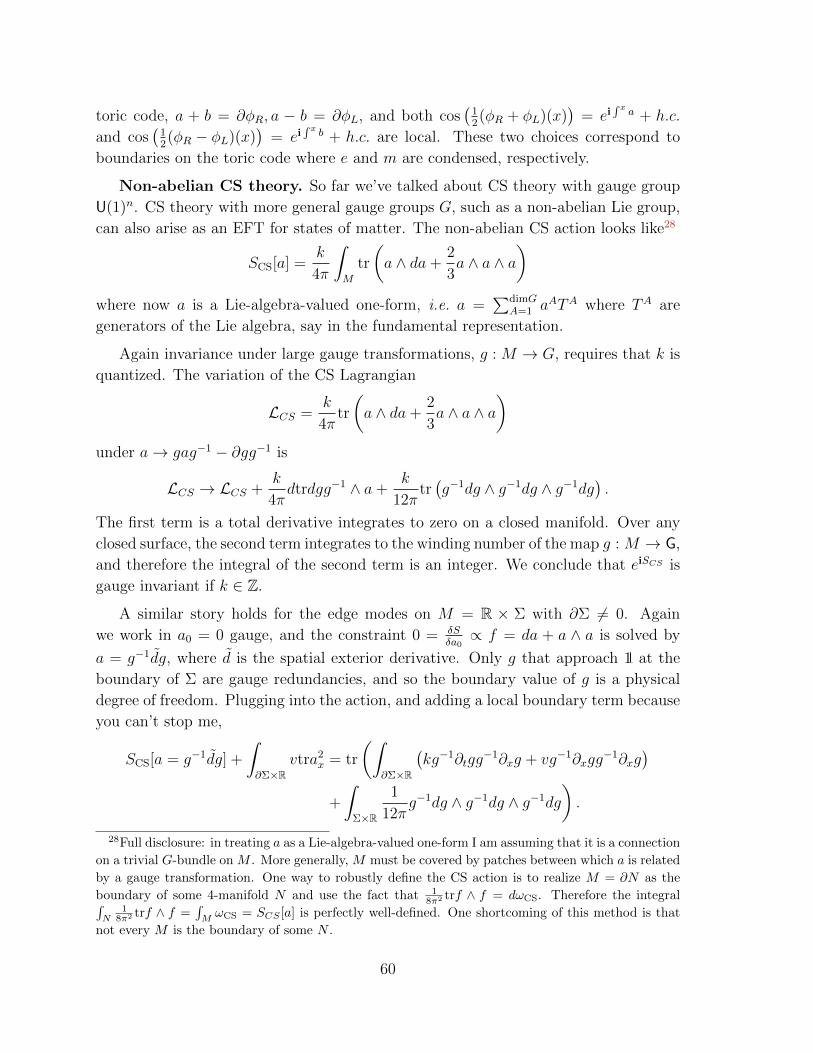
toric code, a + b = ∂φR, a − b = ∂φL, and both cos(
12(φR + φL)(x)
)= ei
∫ x a + h.c.
and cos(
12(φR − φL)(x)
)= ei
∫ x b + h.c. are local. These two choices correspond to
boundaries on the toric code where e and m are condensed, respectively.
Non-abelian CS theory. So far we’ve talked about CS theory with gauge group
U(1)n. CS theory with more general gauge groups G, such as a non-abelian Lie group,
can also arise as an EFT for states of matter. The non-abelian CS action looks like28
SCS[a] =k
4π
∫M
tr
(a ∧ da+
2
3a ∧ a ∧ a
)where now a is a Lie-algebra-valued one-form, i.e. a =
∑dimGA=1 aATA where TA are
generators of the Lie algebra, say in the fundamental representation.
Again invariance under large gauge transformations, g : M → G, requires that k is
quantized. The variation of the CS Lagrangian
LCS =k
4πtr
(a ∧ da+
2
3a ∧ a ∧ a
)under a→ gag−1 − ∂gg−1 is
LCS → LCS +k
4πdtrdgg−1 ∧ a+
k
12πtr(g−1dg ∧ g−1dg ∧ g−1dg
).
The first term is a total derivative integrates to zero on a closed manifold. Over any
closed surface, the second term integrates to the winding number of the map g : M → G,
and therefore the integral of the second term is an integer. We conclude that eiSCS is
gauge invariant if k ∈ Z.
A similar story holds for the edge modes on M = R × Σ with ∂Σ 6= 0. Again
we work in a0 = 0 gauge, and the constraint 0 = δSδa0∝ f = da + a ∧ a is solved by
a = g−1dg, where d is the spatial exterior derivative. Only g that approach 1 at the
boundary of Σ are gauge redundancies, and so the boundary value of g is a physical
degree of freedom. Plugging into the action, and adding a local boundary term because
you can’t stop me,
SCS[a = g−1dg] +
∫∂Σ×R
vtra2x = tr
(∫∂Σ×R
(kg−1∂tgg
−1∂xg + vg−1∂xgg−1∂xg
)+
∫Σ×R
1
12πg−1dg ∧ g−1dg ∧ g−1dg
).
28Full disclosure: in treating a as a Lie-algebra-valued one-form I am assuming that it is a connection
on a trivial G-bundle on M . More generally, M must be covered by patches between which a is related
by a gauge transformation. One way to robustly define the CS action is to realize M = ∂N as the
boundary of some 4-manifold N and use the fact that 18π2 trf ∧ f = dωCS. Therefore the integral∫
N1
8π2 trf ∧ f =∫MωCS = SCS [a] is perfectly well-defined. One shortcoming of this method is that
not every M is the boundary of some N .
60

The first two terms are just like in the abelian case. The third term is still written as a
3d integral, but it only depends on the boundary value of g. It is called a WZW term.
The resulting 1 + 1d field theory is a conformal field theory (CFT) called a chiral Gk
WZW model. The central charge for G = SU(N) at level k is
c =k dimG
k +N.
For non-abelian G, Gk CS theory (at least for k > 1) realizes non-abelian topological
order. For example, SU(2)2 seems to be a description of the (non-abelian) Moore-Read
state (see e.g. p. 45 of this useful review). In case you missed it, last quarter’s class
concludes with a discussion of some bulk observables in non-abelian CS theory.
61

2.3 Representative wavefunctions
You’ll notice that I haven’t said very much about microscopic energetic questions.
Quantum Hall states have been realized by now in many very different materials (in
semiconductor heterojunctions, in other sandwiches made from semiconductors and
insulators and metals, in graphene), and these energetic questions are pretty different
in each case. Part of the reason to avoid that discussion is that it is different in each of
these platforms. Quantum Hall states can even be realized in lattice models without
any external magnetic field, namely Chern insulators. This just means that the hopping
matrix elements are such that the bands have nonzero Chern number. A filled band
with Chern number one has the same effect on the EM response as a filled Landau
level. (I know Dan Arovas talked about Chern numbers last quarter. Should I say
more about this?)
But there is a valuable perspective more microscopic than CS theory, but still more
universal than lattice details, namely representative wavefunctions. By this I mean a
groundstate wavefunction somewhere in the same phase. There is mounting evidence
that the groundstate wavefunction of a gapped phase contains all the universal data of
the phase. This is particularly valuable in the case of quantum Hall states where there
is a topological obstruction to exactly solvable models with exactly zero correlation
length (like the toric code).
How to write down a wavefunction in the right phase? One way is to make an
educated guess, which is what Laughlin did. For times when we are feeling less inspired,
here is a reliable method.
Parton construction. [I recommend Sung-Sik Lee’s TASI 2010 lectures] Here
is a strategy for writing down wavefunctions that represent a phase with topological
order. We have already applied this strategy in the case of nematics. It also produces
a candidate effective field theory, and has many other virtues. It is widely regarded
with suspicion.
A practical point of view on what I’m going to describe here is a way to guess
variational wavefunctions for fractionalized groundstates. A more ambitious interpre-
tation is to think of the parton construction as a low-energy duality between a model of
interacting electrons (or spins or bosons or ...) and a gauge theory of (candidate) ‘partons’
or ‘slave particles’. Like any low-energy duality, it is a guess for useful low-energy de-
grees of freedom. The goal is to describe states in roughly the same Hilbert space29 as
29I don’t mean exactly the same Hilbert space. The construction takes advantage of our ability to
add in ancillary, decoupled, inert bits in changing our representative of a phase. Sometimes condensed
matter physicists use the phrase “the same Hilbert space” to mean up to this equivalence, and it is
in this sense that we mean it here.
62

the original model, in terms of other (hopefully better!) variables. The appearance of
gauge fields (perhaps only discrete ones) is an inevitable side effect when there is frac-
tionalization of quantum numbers (spin-charge separation, fractional charge ...) in D > 1+1.
I will describe the construction in two steps. For definiteness, let’s focus on the
following example. Suppose c to be the annihilation operator for a (spinless) electron
Suppose we are interested in the (difficult) model with
H =∑〈ij〉
(tijc†icj + h.c.
)+∑〈ij〉
V ninj (2.18)
Comments:
1. We’re going to talk about spinless electrons. This is reasonable in a big magnetic
field, which implies a big Zeeman splitting, so that the wrong-pointing spin states
are high energy states we can ignore.
2. We can suppose that the hopping terms tij include some lattice version of the
magnetic field, so tij = teiAij . If you like, you could think of my lattice model
here as just a discretization of electrons in the continuum in a magnetic field.
3. This kind of ‘Hubbard-V interaction’ is the shortest range interaction we can have
for spinless fermions (since the density ni = c†ici is zero or one and so satisfies
n2i = ni).
4. To fully specify the system (2.18), we need to specify the filling – how many
electrons are there per site. If the electrons fully fill some bands and V = 0,
the system is an insulator; since there’s a gap we expect this fact to persist even
for nonzero V . If the filled bands have nonzero Chern number, this is a Chern
insulator, and there is a quantized Hall response. It is just a lattice version of
the IQHE.
5. If we partially fill some Chern bands, without V the system would be a metal.
Interactions have a chance to change that. Indeed such a model can produce
fractional quantum Hall groundstates (on the lattice, such a thing is called a
fractional Chern insulator).
Parton construction: step 1 of 2 (Kinematics)
Relabel states of the many-body H with new, auxiliary variables.
For example, a parton ansatz appropriate to the ν = 13
Laughlin FQH state is
e.g . c = f1f2f3 =1
3!εαβγfαfβfγ
63

fs are complex fermion annihilation operators (they must be fermionic in order that
three of them make up a grassmann operator).
Not all states made by fs are in H. There is a redundancy: if we change
f1 → eiϕ(x)f1, f2 → e−iϕ(x)f2, f3 → f3, or f1 → f1, f2 → eiϕ(x)f2, f3 → e−iϕ(x)f3 ,
(2.19)
then the physical variable c is unchanged. In fact, there is an SU(3) redundancy
fα → Uβαfβ, c→ detUc (of which (2.19) is the Cartan (maximal abelian) subgroup).
We are making the ansatz that c is a baryon.
In any state in H, the number of actual electrons is equal to the number of partons
of each color, since c† creates one of each. The Lagrange multipliers imposing
f †1f1 = f †2f2 = c†c = number of e−; f †2f2 = f †3f3 (2.20)
are the time components a0 of a gauge field.
To write an action for the fs which is covariant under this redundancy, introduce
the spatial components of the gauge field, ai. Perhaps you don’t like this idea since it
seems like we added degrees of freedom. Alternatively, we can think of it as arising from
e− bilinears, in decoupling the c†xcxc†x+icx+i interaction by the Hubbard-Stratonovich
trick. What I mean by this is:
eiV∫dtni(t)nj(t) = eiV
∫dtc†i (t)ci(t)c
†j(t)cj(t)
(2.20)= ei
∫dtV
9
∑α f†iα(t)fiα(t)
∑β f†jβ(t)fjβ(t)
=
∫[Dηαβij ]e
i∫dt∑αβ,〈ij〉
∫dt
(9|ηαβij|2
V+f†iα(t)fjα(t)ηαβij +h.c.
)(2.21)
where η is a new complex (auxiliary) bosonic field on each link. Now let ηij = |ηij|eiaij(for each αβ) and ignore the (massive) fluctuations of the magnitude |ηij| = tij. Voila
the gauge field, and the parton kinetic term.
[End of Lecture 10]
How does the practical viewpoint of constructing possible wavefunctions arise?
Guess weakly interacting partons: Hpartons = −∑
ij tijf†i eiaijfj + h.c. Then fill bands
of f and project onto the gauge invariant subspace.
But what about the fluctuations of a (i.e. we still have to do the a integral)?
Microscopically, a has no kinetic term; in that sense the partons are surely strongly
coupled and confined at short distances (of course they are – the system is made of
electrons if you look closely enough). a only gets a kinetic term from the parton
fluctuations, by processes like this: . The hope is that with enough
64
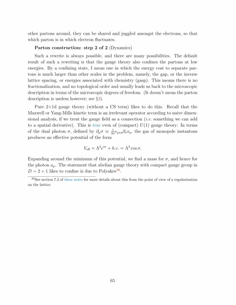
other partons around, they can be shared and juggled amongst the electrons, so that
which parton is in which electron fluctuates.
Parton construction: step 2 of 2 (Dynamics)
Such a rewrite is always possible, and there are many possibilities. The default
result of such a rewriting is that the gauge theory also confines the partons at low
energies. By a confining state, I mean one in which the energy cost to separate par-
tons is much larger than other scales in the problem, namely, the gap, or the inverse
lattice spacing, or energies associated with chemistry (gasp). This means there is no
fractionalization, and no topological order and usually leads us back to the microscopic
description in terms of the microscopic degrees of freedom. (It doesn’t mean the parton
description is useless however; see §3).
Pure 2+1d gauge theory (without a CS term) likes to do this. Recall that the
Maxwell or Yang-Mills kinetic term is an irrelevant operator according to naive dimen-
sional analysis, if we treat the gauge field as a connection (i.e. something we can add
to a spatial derivative). This is true even of (compact) U(1) gauge theory: In terms
of the dual photon σ, defined by ∂µσ ≡ 12πεµνρ∂νaρ, the gas of monopole instantons
produces an effective potential of the form
Veff = Λ3eiσ + h.c. = Λ3 cosσ.
Expanding around the minimum of this potential, we find a mass for σ, and hence for
the photon aµ. The statement that abelian gauge theory with compact gauge group in
D = 2 + 1 likes to confine is due to Polyakov30.
30See section 7.2 of these notes for more details about this from the point of view of a regularization
on the lattice.
65

Let me emphasize again that it’s deconfined
states of parton gauge theories that are most in-
teresting here. So we are looking for gauge theo-
ries which behave oppositely to QCD, really like
anti-QCD, where the partons are deconfined be-
low the confinement scale Λanti-QCD, as in the fig-
ure at right. Interesting states we can make this
way correspond to interesting phases of gauge
theory, a worthy subject.
Our discussion in this section has followed
this diagram starting from the highest energies
(chemistry!) and guessing the lower-energy de-
grees of freedom that result from the interactions
of the constituents. (This dialectic between high-
energy physics and condensed matter physics,
of GUT and anti-GUT, is described vividly by
Volovik.)
Like gaplessness, deconfinement requires an explanation. Known exceptions which
allow for this:
• enough dimensions that the Maxwell term becomes marginal or relevant and we
can have a Coulomb phase.
• partial Higgsing to Zn. Condensing electric charge makes monopoles heavy.
• lots of charged degrees of freedom at low energy. One way to describe their
effects is that they produce zeromodes on the monopole configuration, and the
monopoles only contribute to higher-dimension operators involving insertions of
the light fields. (Interesting constraints on how many modes is enough, from
strong-subadditivity of the entanglement entropy, were derived here. Partons
which are gapless at points in k-space are called algebraic (something) liquids;
the ‘something’ is whatever visible quantum numbers they carry, e.g. spin; if they
happened in this model it would be charge. If the partons form a Fermi surface,
that is certainly enough (Sung-Sik Lee reviews his proof of this in the notes linked
above). This is a kind of spin liquid which may have been observed in various
materials in the past decade or so.
• in D = 2 + 1: the Chern-Simons term a∧ da is marginal, and can gap out gauge
dynamics, as we saw in §2.2, producing a stable, deconfined, topological phase.
If I’ve forgotten some please tell me.
66
Parton construction of Laughlin state. Let’s pursue the Laughlin example a
bit further, but let’s retreat to the continuum. So consider a pile of electrons in 2+1
dimensions, on a space of area A with periodic boundary conditions, in large uniform
B. And let’s put only enough electrons to fill a third of the lowest Landau level. That
is, the number of electrons per lowest Landau level state is
1
3= νe ≡
Ne
NΦ(e)=
Ne
eBA/(hc).
The fact that this band is partially filled means that if the electrons are free, the system
is gapless. But this degeneracy is fragile. Any interaction between the electrons will
split the degeneracy somehow.
If, on the other hand, the electron fractionalizes as c = f1f2f3, then fα carries
charge 1/331. Consider then each fα in the same external field B, and suppose the
partons are free (as a first approximation). Their filling fraction is:
νf =Nf
NΦ(e/3)=
Ne
NΦ(e/3)= 3νe = 1 .
The wonderful thing about this guess is that the partons can now form a gapped
state: that is, we can pretend they are free and fill their bands, so that they make a band
insulator. However, because they are filling a Landau level, this band insulator is an
integer quantum Hall (IQH) state. Then, integrating out the gapped partons produces
a (nonsingular but nontrivial) contribution to the effective action for the gauge field:
the IQH nature of the bands means that there is a Hall response for any gauge fields to
which they are coupled, just as we’ve discussed above. This is encapsulated precisely
by the CS term! 32
31Actually, it is completely arbitrary how we divide up the electron charge amongst the partons;
different choices differ by relabelings of the gauge group which cannot affect the physics.32 We showed that QHE means a CS term earlier. The massive Dirac fermion in 2+1 dimensions also
has a Hall response. The mass term mψψ breaks parity in D = 2 + 1. This slightly-more-microscopic
calculation can be done in just the same manner as the path integral calculation of the chiral anomaly,
and the εµνρ arises for the same reason:
log
∫DψDψ† e
−∫d3xψ
(i /D−m
)ψ
= log det (i /D −m) = Tr log (i /D −m)
≡ Tr log (1− i /D/m) e−2/M2
+ cst 2 ≡ (i /D)2
= −(∂ + a)2 − 1
2Σµνf
µν
= −Tr
∞∑n=1
1
n
(i /D
m
)ne−2/M2
.
where Σµν ≡ 12 [γµ, γν ] is the rotation generator. Now expand the regulator exponential as well and
67

Here is the simplest route to the low-energy theory33. We saw above that a useful
description of the IQHE is in terms of a dynamical U(1) gauge field in terms of which
the current describing the dofs forming the IQH state takes the form j = 12πε∂a, and
the Lagrangian has a term ada4π
. So let’s introduce such a gauge field for each of the
three species of parton:
j(α)µ =1
2πεµνρ∂νb
(α)ρ .
We also have gauge fields associated with the parton gauge redundancy (2.19)34, that
I’ll call a1 and a2. The full effective action is then
4πL =∑α
bαdbα + 2A∑α
qαdbα + 2a1(db1 − db2) + 2a2(db2 − db3) (2.22)
where qα are the electric charges of the partons, which satisfy∑
α qα = 1. a1,2 are just
Lagrange multipliers setting b1 = b2 and b2 = b3. Setting a = b1 = b2 = b3, then, the
action becomes
4πL = 3ada+ 2Ada∑α
qα = 3ada+ 2Ada
which is the effective action we advertised above.
Hence we arrive at a CS theory, like (2.6), for some particular choice of K, de-
termined by the QH response of the partons, i.e. by their charges-squared times the
Chern numbers of their bands.
The Hall conductivity is just sums of the contributions of the partons:
σxy =(e/3)2
h× 3 =
1
3e2/h.
The parton groundstate is |Φmf〉 = P |free parton state〉, where P is the projection
onto the gauge invariant subspace, and the free parton state is obtained just by filling
the lowest Landau levels of the partons. The electron wavefunction is
Ψ(r) = 〈0|∏i
c(ri) |Φmf〉 =
N∏ij
zije−∑Ni |zi|2/(4`2B(e/3))
︸ ︷︷ ︸ν = 1 slater det of charge 1/3 fermions
3
=∏ij
z3ije−∑Ni |zi|2/(4`2B)
the in D = 3, the term that survives the trace over Dirac matrices is
Triaργ
ρ
m
1
M2
((∂ + a)
2+
1
2Σµνf
µν
)= sign(m) trγρΣµν︸ ︷︷ ︸
=ερµν
∫d3x
1
2iaρfµν
33One place in the literature where it appears is see section IV of this paper.34You can ask: what happened to the rest of the SU(3)? One possible answer is that it is sponta-
neously broken down to this U(1)2 subgroup in the state we are describing.
68

where zij ≡ zi − zj. This is the Laughlin wavefunction. (Note that `2B(e) = ~
eB, so
`2B(e/3) = 3`2
B.)
Another route to the low-energy theory is as follows. Just couple the partons to an
SU(3) gauge field a and
integrate out the gapped partons:
∫[Df ] ei
∫L(f,a) = eikCS(a)+···
The resulting low-energy effective field theory of a is SU(3)1 CS theory (with gapped
fermionic quasiparticles). It’s a non-trivial fact that SU(3)1 CS theory with gapped
fermionic quasiparticles is dual to the U(1)3 CS theory that we found earlier – they
have the same groundstate degeneracy and anyon types and bulk response theory. I
hope to explain more about this duality after we speak about invertible phases, since
the derivation essentially involves subtracting an invertible phase from the BHS.
The Laughlin quasiparticle is the parton f with a Wilson line to make it gauge
invariant.
D = 2 + 1 is kind of cheating from the point of view of emergent gauge fields. This
is because the Chern-Simons term is a self-coupling of gauge fields which gives the
photon a mass without the addition of degrees of freedom. We have seen above (in the
toric code example) that this does not necessarily require breaking parity symmetry.
For this reason partons work extremely well to describe QH physics, but they are
also useful for other kinds of quantum matter with strong correlations. For more about
parton gauge theory I heartily recommend Sung-Sik Lee’s TASI 2010 lectures. In his
lectures 2 and 3, he applies this method to bosons and to spins and provides a great
deal of insight.
For a long time I thought that gauge fields were only interesting for condensed
matter physics when deconfinement could be somehow achieved, i.e., when there is
topological order. We’ll see examples in §3 where even confined emergent gauge fields
can do something interesting!
Attempted parable.
The parton construction is a method for ‘solving’ non-holonomic constraints, like
inequalities. In what sense were we solving such a constraint above? Suppose that the
nearest-neighbor repulsion V is the biggest scale in the problem. Then we want the
number of electrons on each pair of neighboring sites to be ≤ 1.
Here is a much simpler example: I can solve the condition y > 0 by writing y = x2.
So we can do a 0-dimensional path integral (integral) over y > 0 in terms of an
69

unconstrained variable x by writing∫ ∞0
dy e−S(y) =1
2
∫ ∞−∞
dx elog |2x|−S(x2).
In this model, the operation x 7→ −x is a gauge redundancy. In this case, it is a finite
dimensional gauge group and we account for it by the factor of 12
out front.
The extra log |2x| term in the action from the Jacobian is like a contribution from
the gauge fluctuations. If I were clever enough I would illustrate deconfinement here,
but I guess that isn’t going to happen in zero dimensions.
The parton construction makes possible
• new mean field ansatze,
• candidate many-body groundstate wavefunctions,
• good guesses for low-energy effective theory,
• accounting of topological ground-state degeneracy and edge states,
• an understanding of transitions to nearby states. (I’ll give an example below.)
It has the following difficulties:
• making contact with microscopic description,
• its use sometimes requires deciding the IR fate of strongly coupled gauge theories.
2.4 Composite fermions and hierarchy states
The following line of thought, which allows us to understand other abelian FQH that
actually occur (at fractions besides ν = 1m
) can be regarded as an important special
case of the parton construction.
Consider what happens as we move away from the center of the plateau where the
filling fraction is exactly 1m
, say by varying the external magnetic field as in the famous
plot. The lowest-energy way to add charge is to create some charge-e/m quasiparticles,
so when we change the filling by a finite amount, we produce some nonzero density of
these objects, still in a large magnetic field. What do they do? They interact with
each other somehow. If they are localized by disorder (i.e. form an Anderson insulator)
or form a Wigner crystal, they Hall conductivity stays at the plateau value. Indeed
at the lowest densities, charged particles with Coulomb interactions do form a Wigner
crystal. But at higher densities, what’s to stop them from forming their own FQH
state?
There are several nice ways to describe this. One is called composite fermions,
70
where the idea is to think of the factors in the Laughlin wavefunction zmij as zijzm−1ij ,
one IQH wavefunction, and one boson ν = 1m−1
(bosonic) Laughlin wavefunction – of
the same variables. Fermi statistics of the electron require Ψ ∝ zij, but the extra m−1
powers are something else. Regard the particle whose wavefunction this is as a fermion
(the one in the IQH state) with m − 1 units of some kind of flux attached (we’ll see
precisely what flux in a moment). Such a particle experiences a reduced magnetic field:
B? = B − (m− 1)ρΦ0. (2.23)
Since the number of such ‘composite fermions’ is the same as the number of electrons,
we have (if B? > 0)
ρ =νB
Φ0
=ν?B?
Φ0
(2.24)
and hence the actual filling ν is related to the filling of composite fermions ν? by
ν =ν?
(m− 1)ν? + 1. (2.25)
If we let the composite fermions fill ν? ∈ Z Landau levels (or fill bands with total Chern
number ν?), we get a gapped state with Hall conductivity given by (2.25). For m = 3,
and ν? = 1, 2, 3 · · · this is
ν =ν?
2ν? + 1=
1
3,2
5,3
7,4
9· · · . (2.26)
You can see these plateaux in the famous plot. This picture suggests a very successful
trial wavefunction for these fillings35, namely:
Ψν(z) = PLLL∏i<j
z2ijΨν?(z, z). (2.27)
Here PLLL is the projector to the lowest Landau level: If we are filling multiple Landau
levels, Ψν?>1 is no longer holomorphic; to make wavefunctions for electrons at ν < 1,
which we expect to be made just from LLL orbitals, we project this thing into the LLL
by the replacement zi 7→ 2`2B∂zi .
Note that there are also such ‘hierarchy states’ with fillings larger than 1m
, which
means B? < 0. In that case (2.24) is replaced by
ρ =νB
Φ0
= −ν?B?
Φ0
(2.28)
so
ν =ν?
2ν? − 1= 1,
2
3,3
5,4
7,5
9· · · . (2.29)
35Define Ψ ≡ Ψe−∑i
|zi|2
4`2B so we don’t have to write the annoying gaussian factor.
71

If we plot the fillings we achieve by this con-
struction (2.26) and (2.29) as a function of
ν?, we get the following plot. This will be
useful later. (Notice that if instead we took
m − 1 to be some other even number as
our starting point, the asymptote would be
ν = 1m−1
instead.)
[End of Lecture 11]
Now here is an explanation of the above numerology in terms of partons. We make
the parton ansatz
c = fb. (2.30)
c is the electron destruction operator, and f and b are fermionic and bosonic partons
respectively. This fractionalization leads to a U(1) gauge field which let’s call a1, under
which f and b have charges 1 and −1. What are the charges of f and b under the
external A? I claim that it does not matter, as long as they add up to one. Now (here
we make a choice), let’s put b into a ν = 1/2 Laughlin state. One way to do that is
to write b = d1d2 in terms of two more fermionic partons, introducing a second gauge
field a2 under which d1,2 have opposite charge (note that it again doesn’t matter how
we distribute the a1 charge between d1 and d2), and let each of d1 and d2 fill a Chern
band. The full table of charges is
A a1 a2
d1 q1 0 1
d2 q2 1 −1
f qf −1 0
Now let’s integrate out d1 and d2. In general, integrating out a field di with charges qαiunder gauge field aα filling chern bands with total chern number ci leads to an effective
Lagrangian
Li =ci4π
∑αβ
(qαi aα) d(qβi aβ
). (2.31)
A useful mnemonic is the following diagram:
α βi
qαi qβi
72

For convenience of writing I’ll call a0 ≡ A, so the couplings to the external gauge field
are included in (2.31). We ignore any other interactions between the partons, so the
contributions of multiple fields just add. So integrating out d1,2 leaves us with
Leff =c1
4π(a2 + q1A) d (a2 + q1A) +
c2
4π(a1 − a2 + q2A) d (a1 − a2 + q2A) + L(f, a)
(2.32)
We can think of these CS terms as attaching flux to the remaining parton f , which is
the composite fermion.
Now we can decide what to do with f ; depending on what we do, we’ll find different
states, with different Hall response. If we let f fill Chern bands with total Chern number
ν?, we can integrate out f , too, in the same way, and get Leff =∑
i Li with Li as in
(2.31). If we set ν? = 1 we reproduce exactly our earlier construction of the Laughlin
state. To find the general Hall response, we can just solve the equations of motion for
a1,2; these are linear equations that determine a1,2 in terms of A. Plugging back into
(2.32) then gives an action of the form L = ν4πAdA with, setting c1 = c2 = c36,
ν =cν?
c+ 2ν?. (2.33)
If I set c = 1, this is exactly (2.26). And the parton trial wavefunction is just (2.27).
Hierarchy and K-matrices. There is another way to construct the hierarchy, by
combining the logic with which we began §2.2 with the picture with which we began our
discussion of the hierarchy states. So we’ve argued that the EFT in terms of CS gauge
fields is an inevitable consequence of U(1) symmetry, a gap, and broken time-reversal
symmetry. That’s the same situation we’re in when we add a density of quasiparticles
to move away from the center of the plateau (assuming we make a gapped state). So
the same logic suggests that we write also the quasiparticle current
jµqp =1
2πεµνρ∂ν aρ (2.34)
in terms of a (new) CS gauge field! You can’t stop me. The minimal-coupling term
aµjµqp becomes a mixed CS term. The full action (epsilon tensors are implicit) is
4πL = kada+ 2Ada+ 2ada+ kada+ · · · ,
where I’ve added a CS term to describe the dynamics of the quasiparticles, by the
same logic as before. This is of the form (2.6) with a 2 × 2 K-matrix, K =
(k 1
1 k
)36In this calculation, it is an extremely useful check to leave the electric charges of the partons
arbitrary, and make sure that the answers only depend on the sum of their charges, which is fixed by
the charge of the electron.
73

with charge vector t = (1, 0). If we integrate out a and a in this action, we’ll find Hall
conductivity
ν =1
k − 1k
.
If k = 2, we reproduce our previous hierarachy states. These FQH states of compos-
ite fermions are observed here here. This CS description determines the groundstate
degeneracy (to be | detK|g on a genus-g surface) and the charges and statistics of the
quasiparticle excitations above this state: minimally couple particles to a and a. The
quasiparticle charges that one computes this way are observed experimentally, e.g. at
ν = 25.37
Now, why should we stop here? Moving away from the middle of the plateau of one
of these states, there is a density of those quasiparticles whose charges I just mentioned.
Why can’t they, too, form a QH state? Then we would write their current in terms of
yet a third CS gauge field, and we would arrive at a description with a 3×3 K-matrix,
and a Hall conductivity that was a continued fraction with a third level. You can also
see these states in clean samples.
This construction gives K-matrices with integers on the diagonal and ones on the
next-to-diagonal. The K-matrix K =
(m1 n
n m2
)and charge vector t = (1, 1) also de-
scribes states that exist (named after Halperin), and whose filling fraction, quasiparticle
data and GSD you can now compute.
We can relate theories with different K-matrices by a relabelling of fields, aI →W IJa
J . But in order to preserve the flux quantization, the matrix W must have
| detW | = 1, that is W ∈ GL(n,Z). Thie resulting equivalence relation acts by
KIJ → W IKK
KLW JL , tI → W I
J tJ . (2.35)
Quantum Hall Metal. Now comes some real magic: look again at the limit as
ν? → ∞ of the plot above. What happens when ν = 12
(or more generally ν = 1m−1
)
in the composite fermion construction? Look at (2.23): when ν = 1m−1
, the composite
fermion sees no magnetic field at all! This is despite the fact that half-filling happens
(for realistic electron densities in a 2DEG) at enormous magnetic fields like 25 Tesla.
This suggests that in our parton ansatz (2.30) the composite fermion f can just fill a
Fermi sea, and would move in straight lines in response to an external electric field.
This would be a gapless, metallic state. And indeed that is what is seen near ν = 12!
37A nice resource for the literature on experimental studies of FQHE up to 2004 is the slides of
Willett here.
74

A trial wavefunction for this amazing state is then just
Ψ(z) = PLLL∏i<j
z2ij det
ijeiki·rj (2.36)
where the ki label the N lowest energy modes. I think this wavefunction was first
written down by Read and Rezayi, but Halperin, Lee and Read explained a lot of the
physics, so I call it the HLR state. A similar story occurs (in experiments as well) at
other fillings of the form ν = 1m−1
for m an odd number.
But there’s more: let’s start at the HLR state at ν = 12
and vary the magnetic field
(at fixed electron density) away from the special value where the composite fermions see
no field B = Bν= 12+δB. What happens when we subject a Fermi surface to a magnetic
field? We get quantum oscillations: various quantities, including the conductivity, are
periodic with period 1/δB. But this periodic structure is exactly where the hierarchy
plateaux appear! (That is: if 1δB
= ± ν?
ρΦ0for some integer ν?, the actual filling fraction
is ν = ν?
2ν?±1.) This means we can regard all of the hierarchy states, including the
original Laughlin states, as extreme manifestations of quantum oscillations.
Notice that the composite fermions at the Fermi surface still interact with a Chern-
Simons gauge field. This is a non-Fermi liquid: a metallic system that is not described
by ordinary Fermi liquid theory.
Incompressible states at even denominators. Finally, one thing that fermions
at a Fermi surface like to do is pair up and superconduct. What happens if the
composite fermions in the HLR state form a superconductor? Well, by Fermi statistics,
it has to be a p-wave superconductor because the composite fermions are spinless (we’re
assuming the electrons are completely spin-polarized). If they form a p+ ip (nodeless)
superconductor, the projection of the BCS wavefunction is the Moore-Read state, which
is a non-abelian topological order. (Perhaps more on this wavefunction later. This is
not how it is was first discovered.) Whether or not the composite fermions pair up
depends on the consequences of the CS interactions, and on microscopic details. (For
an analysis of this drama, see here.) In the half-filled lowest Landau level, we see a
metallic state, but in the half-filled third Landau level (i.e. at ν = 52), there is indeed
an incompressible state, which could be the Moore-Read state. (At ν = 32, 7
2, one finds
instead states that break translation symmetry – stripes.)
Recently there has been some further development in our understanding of what
happens near ν = 12. The state (2.36) makes a distinction between a half-full and a
half-empty Landau level – it is not symmetric under the interchange of particles and
holes. But experiments show that the physics is particle-hole invariant. Sonuggested
a way to write down a particle-hole symmetric state by starting with Dirac composite
fermions, rather than the non-relativistic ones that I’ve been talking about. This line
75

of inquiry has also had some important consequences for our understanding of the
gapped and likely non-abelian state at ν = 52. Recent measurements (of thermal Hall
conductivity (which counts the number of edge modes, including neutral ones) and of
interfaces with other states) favor a particle-hole symmetric version of the Moore-Read
state (called the PH-Pfaffian).
Transitions to neighboring phases. What happens if the Chern numbers of the
bands occupied by the partons d1,2 are not both 1 (let’s call it (c1, c2) = (1, 1))?
It is not hard to describe a transition where Chern numbers
change: just vary the bandstructure until the bands touch
at a Dirac point. Moving past that point, the two touch-
ing bands exchange Chern numbers. (I like to think of it
like a crossover event during meiosis. The pictures are very
similar.) If one is filled and one is empty, this will change
the resulting contribution to the Hall response. For example,
imagine that in the figures at right the blue band is filled.
And we see that a theory of the transition is a Dirac fermion
coupled to Chern-Simons gauge fields.
[End of Lecture 12]
Consider just the theory of a boson b, with the ansatz b = d1d2, where d1 and d2
fill Chern bands with Chern numbers (c1, c2). The effective Lagrangian for the gauge
field a1 gluing them together is
L =c1
4π(a1 + q1A) d (a1 + q1A) +
c2
4π(−a1 + q2A) d (−a1 + q2A) . (2.37)
Integrating out a1 gives Hall response
νb =c1c2
c1 + c2
. (2.38)
Several cases are interesting. If (c1, c2) = (1, 0), the calculation above gives ν = 0, no
Hall response. But the state of the boson b = d1d2 is still an insulator, there is still an
energy gap. This is a (weird!) description of a featureless Mott insulator.
Another very interesting case is when (c1, c2) = (1,−1), in which case (2.38) blows
up. This is a signal that the theory is actually gapless. In fact it is a dual description of
the superfluid phase of the boson. To see this, go back to (2.37). When c1 = −c2 = 1,
76

it reduces to
L =1
2πadA+ f 2 (2.39)
which says that there is no CS term for a, and I’ve added back the Maxwell term,
since it’s now the leading term governing the dynamics of a. Earlier I said that pure
compact U(1) gauge theory in D = 2 + 1 confines because of monopole instantons.
But the first term in (2.39) says that magnetic flux of a carries charge under the U(1)
global symmetry. This means the operator eiσ is not U(1) symmetric (σ shifts) and
can’t be added to the action. This describes a gapless theory, where the photon is the
goldstone boson, ∂a = ε∂σ, for spontaneously breaking the U(1) symmetry.38
In the presence of some lattice symmetry (like parity, k →−k) that forces two band-touching points at the same point
in the phase diagram, it can force the Chern number of the
filled band to change from c = −1 to c = 1. If this happens
to d1 (fixing c2 = 1) we have a direct transition from the
Laughlin ν = 12
state to a superfluid. Notice that the critical
theory involves two species of Dirac fermions.
We can thereby produce
a boson phase diagram
that includes these three
phases.
(The state with (c1, c2) = (−2, 1) is also interesting – it is a
boson IQH state with ν = 2.)
Now we can use this to make a theory of electronic transitions out of the HLR
phase, for example to a Mott insulator. In our description of the HLR phase, the Hall
response comes entirely from that of b. When b goes from the ν = 12
state to the Mott
insulator, the full electron state goes from HLR to a (fermionic) Mott insulator. (And
indeed, the general formula, if f also fills Chern bands with Chern number ν?, is
ν =c1c2ν
?
(c1 + c2)ν? + c1c2
. (2.40)
Again if (c1, c2) = (1, 0), we find no Hall response.)
38Another way to think about (2.39) is to integrate out a and see what effective action we get for A.
The equation of motion says roughly ∂2a ∼ ∂A, and plugging back in we get Leff[A] ∼ A∂(
1∂2
)∂A ∼
A2, a Meissner mass for A, as we should have in a superfluid.
77

With the fractionalization c = bf , if b instead forms a super-
fluid state, it completely higgses the U(1) gauge field gluing
together b and f . The result is that we can forget about both
b and the gauge field, and we get an ordinary Fermi liquid. So
in this way we can describe a phase diagram containing the
HLR state, Mott insulator and ordinary metal. You could
imagine moving around in such a phase diagram by applying
a periodic potential to a 2DEG, at fixed electron density and
magnetic field.
78

3 Symmetry-protected topological phases
We begin with a low-tech example-based response-theory point of view on symmetry-
protected topological (SPT) states. Sources for this discussion include Senthil’s review.
Useful and brief is the second part of this review. See also this Journal Club for
Condensed Matter Physics commentary by Matthew Fisher.
We are interested in possible ways to distinguish phases of quantum matter (without
having to check every possible adiabatic path between them in the infinite-dimensional
space of Hamiltonians). Here is a simple yet still-interesting question (which has been
very fruitful in the past decade or so): how do we distinguish phases of matter that
preserve their symmetry group G but don’t have topological order?
One possible answer: put them on a space with boundary, i.e. an interface
with vacuum or with each other. Quantized (hence topology) properties
of the surface states can be characteristic of distinct phases.
The rough (and not entirely correct) idea is: just like varying the Hamil-
tonian in time to another phase requires closing the gap H = H1 +g(t)H2,
so does varying the Hamiltonian in space H = H1 + g(x)H2. (We’ve al-
ready seen an exception to this in the interface between the toric code
and vacuum.)
Notice that the possibility of characterizing a state in this way requires that the
D − 1-dimensional edge theories involved must not be realizable intrinsically in D − 1
dimensions, consistent with the symmetries involved. If they could be so realized,
preserving G, we could paint them on the surface of any bulk state, and they therefore
could not be characteristic of the bulk state. Therefore there is a correspondence
between SPTs in D dimensions and obstructions to symmetry-preserving regulators of
quantum field theory (QFT) in D − 1 dimensions.
Definition: a gapped groundstate of some local Hamiltonian H preserving G without
topological order, and which is distinct from any trivial product state in the space of G-
symmetric Hamiltonians, is called a SPT (symmetry-protected topological) state with
respect to G. (There are some subtleties with this definition to which we’ll return.)
Inevitably I will also use the term ‘SPT’ for the phase of matter of which such a
groundstate is a representative.
79

The deformation classes of SPT states form a
group. The group law is stacking. Stacking A and
B means we make the system whose Hilbert space
is the tensor product of those of A and B, and
whose Hamiltonian is the sum. (Then we are al-
lowed to deform the Hamiltonian, preserving the
gap, as usual.) The inverse of a state A, which
we can call −A, is (usually) the mirror image. A
cartoon of why this is the case is given at right.
' ∅
To be clearer, the definition of the inverse state of A is a state with the property
that there exists a finite-depth unitary circuit U such that
U |ψA〉 ⊗ |ψ−A〉 = product state. (3.1)
Please don’t take the cartoon too seriously; its main point is to show that the edge
modes can be cancelled. In fact, if we consider a state with gapless edge modes on
a space with boundary, the operation (3.1) cannot be done with a finite-depth circuit
(by the Lieb-Robinson bound) – it’s only on a closed spatial manifold that we demand
(3.1). Note that with topological order, even if we can gap out the edge states, there is
still stuff going on (e.g. anyons) in the bulk, and no such ψ−A or U exist: states with
topological order do not form a group under stacking.
Naturally, a state that has an inverse is called invertible. It would have been wise of
me to define SPTs to be invertible states, and I will do so below. In any case, one can
ask whether the absence of topological order, for example the vanishing of the topo-
logical entanglement entropy (TEE) is sufficient to imply the existence of an inverse
state. A sketch of why this might be the case is the following: a nonzero TEE is an
obstruction to the reconstruction of the global groundstate from the density matrices
on subsystems. If all TEEs vanish, in a system with no edge states (such as A plus
its mirror image with gapped boundary conditions), we can therefore assemble the
full groundstate wavefunction by the following procedure, starting from the state on
an array of balls (each large compared to the correlation length), which we’ll call the
0-skeleton.0-cell 1-cell
2-cell
Then we can connect these balls by tubes (also topologically
balls) acting like 1-cells in a cell complex; then we can glue
in 2-cells, and so on. The resulting process defines a finite-
depth unitary circuit, and the idea is that TEE and edge
modes are the only obstructions to doing this. (More details
can be found in §3.1 here. A related construction is described
here, in section 1.2.).
How to characterize these states more precisely? Many possibilities have been
80
explored so far. To get started:
1. If G ⊃ U(1), we can study the response to an external electromagnetic (EM)
field. Just like the integer quantum Hall effect, this will involve some quantized
coefficients.
Without a U(1) (or other continuous symmetry), we need something else. (And two
states with the same quantized EM response may be distinct for some other reason.)
2. What happens if you gauge G? In general this produces a new state, with TO
(or gapless). That state can be used as a label on the SPT. (This works both
ways: labelling TO or gapless states is the hard part.) I’m not going to say more
about this here.
3. Weird, seemingly-forbidden stuff at the surface. For example, the surface could
have half-integer Hall response, but no topological order. Or the surface can
have patterns of fractionalization that violate associativity constraints. The gen-
eral name for these phenomena, which mean that the effective action of the edge
theory is not gauge invariant, is anomalies. And the phenomenon where the pres-
ence of the bulk theory allows for would-be-impossible things on the boundary,
is called anomaly inflow.
[End of Lecture 13]
This concept of anomaly has many manifestations. A useful basic definition of
an anomaly is any obstruction to gauging a symmetry, that is, to treating the back-
ground fields as dynamical variables. The name comes from high energy physics. The
perspective there is that there can be symmetries of the classical action that are not
symmetries of the path integral (i.e. of the path integral measure). We’ll have an
occasion to review some examples of this in a bit.
Since anomaly is defined to mean some failure of gauge invariance of the effective
action, you can already see that it has a close connection to the LSMOH ideas.
The definition above gives a group of SPTs for each choice of symmetry group
G and dimension d. This group is abelian. What can it be? Essentially using the
Landau what-else-can-it-be method for suitably-general choices of background fields,
this group has been determined. It is the Anderson dual of the G-equivariant bordism
group in d + 1 dimensions. Later I will try to make some of these words meaningful.
For now, I want to convey the nature of this classification: what’s been classified is the
effective actions of the background fields. The classification we have does not produce
representative wavefunctions.
81

Perhaps I should emphasize here that there is an important divide between SPTs
that are made from only microscopic bosons, where the Hilbert space is a tensor prod-
uct, and SPTs with microscopic, gauge-invariant fermions, where distant local opera-
tors are allowed to anticommute. With even free fermions, there are many examples of
SPTs (called topological insulators) realized by topological bandstructure. In contrast,
SPT states of bosons (especially in D = 3 + 1) are particularly interesting partly be-
cause they require interactions. (Non-interacting bosons just form a boring superfluid.)
Note that ‘states of bosons’ also means states of spins by a simple mapping of states.
Why study SPTs? For me, the point of studying SPT states is several-fold.
The general question being asked here is basically: how can symmetries be realized on
many-body systems? Clearly this is an interesting question of broad applicability.
One motivation is that by understanding all the ways in which symmetries can be
realized in quantum systems, we can learn how to gauge them, and thereby make new
states with topological order. Are all topologically-ordered states obtained this way?
Maybe not. (e.g. how to think about fibonacci anyons in this language? Actually the
parton construction produces a gauge theory that can be regarded as gauging an SPT.)
A second reason is that each SPT state in D dimensions represents an obstruction to
regularizing a QFT in D− 1 dimensions with certain properties. Such a QFT does not
come from a local, symmetric lattice model. A famous example of such an obstruction
is the Nielsen-Ninomiya fermion-doubling theorem. Some new anomalies have been
found this way. This perspective has also added some new vigor to the quest to define
the Standard Model (a chiral gauge theory) on the lattice.
One outcome of this direction is that the surface of an SPT facilitates the emergence
of supersymmetry from a lattice model. Supersymmetry is a great idea still looking
for its place in nature. The basic idea is that the supersymmetric fixed point has two
relevant deformations, but one of them is forbidden by a funny (SPT-edge) realization
of time-reversal symmetry.
Finally, a zeroth-order reason to study SPTs is that they exist. If we are going to
understand all phases of matter, we need to understand them.
3.1 EM response of SPT states protected by G ⊃ U(1)
3.1.1 D = 2 + 1, G = U(1)
This is what we did in §2.1. Our conclusion was σxy = limω→0〈jxjy〉|k=0
iω= ν e
2
h= ν
2π,
and ν is quantized if there is no fractionalization (and ν is even in a model of bosons
without fractionalization).
82

On the other hand, even without TO, the integer ν provides a label on a phase of
matter, since it cannot vary continuously.
3.1.2 K-matrix construction of SPT states in D=2+1
Let’s talk about effective-field-theory realizations of such states.
(This discussion is from here.) Recall our description of abelian FQH states, with
effective action
S[aI ] =∑IJ
KIJ
4π
∫aI ∧ daJ .
The actual particle (electron or boson) current, representing the global U(1) symme-
try, is Jµ = 12πεµνρ∂νa
IρtI . That is: coupling to the external gauge field is ∆L =
AtIε∂aI/(2π). We showed that this produces a Hall response
σxy =1
2πt−1K−1t.
The number of groundstates on a genus-g surface is | detK|g. If we choose K with
| detK| = 1, this suggests that there is no topological order. We can check that this
is the case by examining the spectrum of quasiparticles. Quasiparticles are labelled by
an integer vector lI specifying their coupling to aI .
self (exchange) statistics: θ = πlTK−1l .
mutual statistics: θ12 = 2πlT1 K−1l2.
external U(1) charge of quasiparticle l: Q = tTK−1l.
To make an SPT state, we must ensure that all these quantum numbers are multi-
ples (not fractions!) of those of the microscopic constituents.
To describe a boson IQH state, consider K = σx. Think of the two states as like
two ’layers’ or species of bosons, so we can take statistics vectors l1 = (1, 0), l2 = (0, 1).
These are self bosons and mutual bosons. If we take the charge vector to be t = (1, 1)
(both species carry the charge) then this state has ν = 2.
For ν = 2 boson IQH: K = σx, t = (1, 1). Let’s put the system on the lower-half
plane and look at the edge theory. Writing it in terms of the eigenvectors φ± of K, we
have
SCS[aI = dφI ] =1
4π
∫dtdx
(∂tφ
+∂xφ+ − ∂tφ−∂xφ− + v
(∂xφ
±)2)
This shows that φ± ≡ 1√2
(φ1 ± φ2) are left- and right-moving respectively.
83
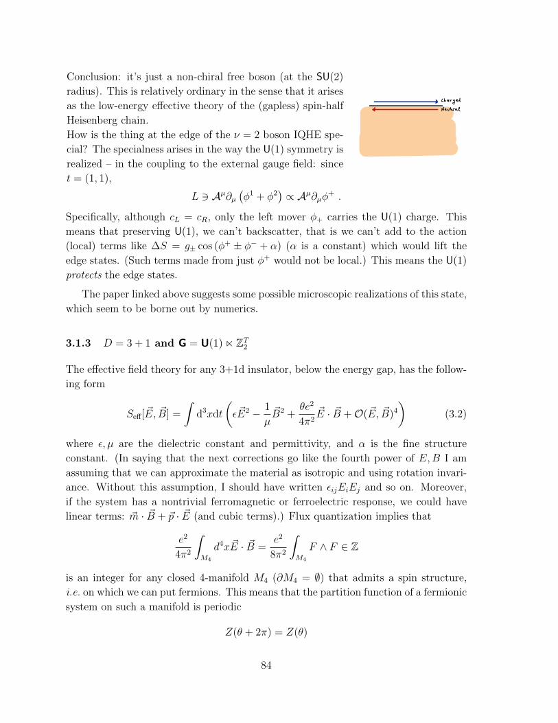
Conclusion: it’s just a non-chiral free boson (at the SU(2)
radius). This is relatively ordinary in the sense that it arises
as the low-energy effective theory of the (gapless) spin-half
Heisenberg chain.
How is the thing at the edge of the ν = 2 boson IQHE spe-
cial? The specialness arises in the way the U(1) symmetry is
realized – in the coupling to the external gauge field: since
t = (1, 1),
L 3 Aµ∂µ(φ1 + φ2
)∝ Aµ∂µφ+ .
Specifically, although cL = cR, only the left mover φ+ carries the U(1) charge. This
means that preserving U(1), we can’t backscatter, that is we can’t add to the action
(local) terms like ∆S = g± cos (φ+ ± φ− + α) (α is a constant) which would lift the
edge states. (Such terms made from just φ+ would not be local.) This means the U(1)
protects the edge states.
The paper linked above suggests some possible microscopic realizations of this state,
which seem to be borne out by numerics.
3.1.3 D = 3 + 1 and G = U(1) n ZT2
The effective field theory for any 3+1d insulator, below the energy gap, has the follow-
ing form
Seff[ ~E, ~B] =
∫d3xdt
(ε ~E2 − 1
µ~B2 +
θe2
4π2~E · ~B +O( ~E, ~B)4
)(3.2)
where ε, µ are the dielectric constant and permittivity, and α is the fine structure
constant. (In saying that the next corrections go like the fourth power of E,B I am
assuming that we can approximate the material as isotropic and using rotation invari-
ance. Without this assumption, I should have written εijEiEj and so on. Moreover,
if the system has a nontrivial ferromagnetic or ferroelectric response, we could have
linear terms: ~m · ~B + ~p · ~E (and cubic terms).) Flux quantization implies that
e2
4π2
∫M4
d4x~E · ~B =e2
8π2
∫M4
F ∧ F ∈ Z
is an integer for any closed 4-manifold M4 (∂M4 = ∅) that admits a spin structure,
i.e. on which we can put fermions. This means that the partition function of a fermionic
system on such a manifold is periodic
Z(θ + 2π) = Z(θ)
84

and hence the spectrum on a closed 3-manifold (M4 = S1 ×X3 is spin) is periodic in
θ. (As we will discuss, shifting θ by 2π is not so innocuous on a space with boundary
or for the wavefunction.)
Time reversal acts by
T : ( ~E, ~B)→ ( ~E,− ~B)
which means θ → −θ, which preserves the spectrum only for θ ∈ πZ. So fermionic time-
reversal-invariant insulators are labelled by a quantized ‘magneto-electric response’
θ/π = 1.
Now consider what happens on a space with boundary, like
for any actual chunk of material. The interface with vacuum
is a domain wall in θ, between a region where θ = π (TI) and
a region where θ = 0 (vacuum).
Letting θ depend on space, the electromagnetic current derived from (3.2) is
jµEM = − e2
8π2εµαγδ∂αθ∂γAδ + · · · (3.3)
where the · · · indicate contributions to the current coming from degrees of freedom
at the surface which are not included in (3.2). If we may ignore the · · · (for example
because the edge is gapped), and approximate ∂zθ = ∆θδ(z), then we find a surface
Hall conductivity (restoring units 2π = h)
σxy =e2
h
∆θ
2π=e2
h
(1
2+ n
)(3.4)
where ∆θ, the change in θ between the two sides of the interface, is a half-integer
multiple of 2π.
In terms of the edge theory, the periodicity in θ ' θ + 2π for the fermion TI can
be understood from the ability to deposit an (intrinsically 2+1 dimensional) integer
quantum Hall system on the surface. This changes the integer n in the surface Hall
response (3.4).
85

Parallel with polarization. There is a nice parallel between this connection
between the bulk ambiguity in θ and the possibility of depositing IQHE layers on the
surface and the theory of electric polarization. The polarization P of a (say 1d) crystal
is a periodic variable, because shifting every electron by a lattice spacing takes the
crystal back to itself in bulk. In the presence of a surface, this shift removes charge
from one surface and deposits it on the other surface. Indeed, a good understanding
of polarization is in terms of the Berry connection39. Very roughly, this is because
polarization is the density of electric dipoles e 〈~r〉 ∼ e∫k
⟨i~∇k
⟩= e
∫k~A(k).
[End of Lecture 14]
And indeed, there is a D = 1 + 1 analog of the story above: Consider an insulator
in D = 1 + 1 with U(1) symmetry and a Z2 charge-conjugation symmetry, under which
jµ → −jµ. The effective action for the background gauge field can have a term of the
form
Sθ[A] =
∫X2
θ
2πF. (3.5)
You can see that P = θ2π
, since the coupling of an electric dipole is ~d · ~E, and P should
be the dipole density.
39More precisely, the polarization can be obtained as an integral over time of the current that
produces it: d~Pdt = ~j. Now imagine varying some parameter λ in H to produce adiabatically such a
polarization. First order perturbation theory says the change in the state of the nth band is
|δψnk〉 = −i~λ∑m6=n
〈ψmk|∂λψnk〉Enk − Emk
|ψmk〉 .
The contribution to the resulting current is
~jn =d~Pndt
=
⟨e~p
m
⟩n
=i~emλ∑m6=n
∮BZ
ddk〈ψnk| ~p|ψmk〉〈ψmk|∂λψmk〉
Enk − Emk+ h.c.
Now use Bloch’s theorem to write ψnk(r) = eik·runk(r), with unk(r) periodic, which satisfy Hk |unk〉 =
Enk |unk〉 with Hk = (p+~k)2
2m + V . Therefore ~p = m~~∇kHk −~k. Expanding the eigenvalue equation to
first order in δk to eliminate ∂kH leads to some juicy cancellations and gives
d~P
dλ= ie
∑n,occupied
∮BZ
ddk⟨~∇kunk|∂λunk
⟩+ h.c.
The polarization is therefore
~P =
∫ 1
0
dλd~P
dλ= eIm
−i ∑n,occupied
∮BZ
ddk ~Ann(~k)
where ~Amn(k) ≡ i 〈umk| ~∇k |unk〉 is the Berry connection.
86

Because of flux quantization, Z(θ) = Z(θ + 2π) on a closed manifold. Microscopi-
cally, θ =∮
dk∑
n,occupiedAnn is just the Berry connection. It is periodic because under
a rephasing of the wavefunction unk(r) → g(k)unk(r), A → A + g−1∂kg changes by
a gauge transformation. The choice g(k) = eimak for m ∈ Z (where a is the lattice
spacing) shifts θ by 2π.
Under the charge conjugation symmetry, F → −F . The allowed values of θ, then,
are θ = 0, π. In the presence of a domain wall connecting the two phases, the EM
current has a contribution jµ = εµν ∂νθ2π
, which says that there is a half-unit of charge
localized at the wall.
Note, by IBP, the similarity between the polarization term (3.5) and Sν [θ, A] =∫ν2πdθ ∧ A in our theory of elasticity! In fact, the most current, many-body under-
standing of electric polarization in general dimension d is in terms of a term just like
our d-dimensional term
Sν [θI , A] =
ν
(2π)dd!
∫A ∧ dθI1 ∧ · · · ∧ dθIdεI1···Id . (3.6)
The role of the polarization vector is played by ~P =~θ
2π40. More generally, the point
in life of the term (3.6) is to encode the response to flux-threading. It is sometimes
said that (3.6) is like an unquantized anomaly, since P itself need not be an integer.
But, as we saw earlier, the coefficient ν is an integer if the action needs to be invariant
under large gauge transformations (i.e. if there’s no groundstate degeneracy).
While I’m talking again about Sν I have to mention something else that it encodes,
called the Thouless quantized charge pump. It is closely related to the presence of the
fractional surface charge. Consider the case of D = 1+1. Suppose we can adiabatically
vary the coupling parameter θ n times through its period, θ → θ + 2πn, during some
time interval T . What amount of charge Q passes a given point in the bulk? The
current is jµ = ν2πεµν∂νθ, so
∆Q =
∫ T
0
dtjx(t) =
∫ T
0
dt∂tθν
2π=
ν
2π
∮dθ = νn. (3.7)
So, under the by-now-familiar assumptions that quantize ν, the charge transported in
an adiabatic loop is quantized. (Note that when the parameter θ2π
is interpreted as
the polarization, this conclusion becomes a bit tautological.) We’ve already seen an
40Note that in the reference above, the term is described in terms of Z gauge fields. These are
somewhat-mysterious objects whose properties are identical to those of dθI (they encode the size and
shape and defects of the lattice, in that e.g.∮Cidθi = Li, and d2θi
2π is the density of dislocations with
Burgers’ vector i). The intended advantage of the formulation in terms of the more-mysterious Zgauge fields is that they carry less information than a configuration of θI , which also carries geometric
data. In practice however I think it’s always necessary to pick an analog of the θI anyway.
87

example of this in Laughlin’s argument around (2.4) – consider the limit where the
annulus is a thin tube, so it looks like a 1d wire. Generalizations to higher dimensions,
closely related to (3.6) are discussed here.
Polarization from monopole quantum numbers. Plugging in θI → θI +2πP I
to (3.6) gives
Spol =d∑i=1
(−1)i+1P i
∫x1 ∧ · · · xi−1 ∧ dA ∧ xi+1 ∧ · · · ∧ xd (3.8)
where xi ≡ dθi
2πare the Zd gauge fields associated to lattice translations. Let’s ask how
this action responds to the insertion of 2π flux.
1. In D = 1 + 1, insertion of 2π flux is an event in spacetime described by F =
2πδ2(x⊥), and this produces a phase Spol = 2πP .
2. In D = 2 + 1, 2π flux is a particle, with a worldline on which F = 2πδ2(x⊥) has
support. The term evaluates to
Spol =
∫worldline
dt2π (P x∂tθy − P y∂tθ
x) . (3.9)
What does this do? Consider the canonical momentum for θi:
Πi ≡ δS
δθi(x)= · · ·+ 2πεijP j (3.10)
where the · · · are contributions from other terms. The generator of lattice trans-
lations in the i direction is
T i ≡ eiΠi
= T i0 e2πiεijP j .
This says that 2π flux carries lattice momentum
~k = 2π(−P y, P x).
We can therefore infer the polarization by measuring the momentum (phase ac-
quired by unit translation) of the state in the presence of 2π flux.41
41Some more telegraphic comments connecting this point to other ideas: The fact that flux can
carry lattice momentum was realized long ago by Haldane and by Read and Sachdev, and plays
an important role in the Neel-to-VBS transition on the square lattice (the skyrmion of the AFM is
realized in the NCCP1 description as 2π flux, and the fact that it carries lattice momentum is why
its condensation produces a state that breaks translation symmetry, the VBS phase). More generally,
this idea was used by Song-He-Vishwanath-Wang (the same authors in an earlier paper) to provide
an understanding of the lattice-symmetry-breaking phases of a system containing an algebraic spin
liquid. Those phases are described by the condensation of monopoles; the monopole quantum numbers
therefore determine the lattice symmetries that are broken.
88

3. In D = 2+1, the insertion of 2π flux is still codimension two, so it happens along
the worldsheet of a string. The endpoint of such a string is a magnetic monopole.
The polarization term evaluates to
Spol =
∫worldsheet
dtdx2πεijkP i∂tθj∂xθ
k. (3.11)
This changes the canonical momentum of θj by
Πj = · · ·+ 2πεijkP i∂xθk.
The consequence is that acting on the 2π-flux string, the translation operators
satisfy
T xT y = T yT xe2πiP z .
This is the magnetic translation algebra for a particle with charge q in a magnetic
field B, with 2πP z = qB.
This phenomenon is closely related to the magneto-electric response in (3.2), as
follows. As I mentioned, one way to think about the θ angle is
θ ∝ ∂P
∂B=∂M
∂E.
Upon turning on a magnetic field, we should have
∆~P =θ
4π2~B. (3.12)
But as we’ll see below, in the presence of nonzero θ, a magnetic monopole carries
electric charge q = θ2π
. This means that when we turn on Bz, the monopole
behaves like an electric charge in a magnetic field, and so the magnetic translation
algebra should obtain, with an extra contribution
2π∆P z = qBz =θ
2πBz,
which is (3.12).
In D = 2+1 we had a very general argument that fractional Hall response required
fractionalization. There is an analogous theorem about the magneto-electric response
in T -invariant systems: in the absence of fractionalization, θπ
must be an integer for a
gapped T -invariant system.
89

Here’s the argument: Put the system on T 3, and apply a tiny magnetic field ~B =
Bz, uniform in x, y, so that∫dxdyeBz = 2π, the minimal flux. I say that this is
tiny to emphasize that this time-reversal-breaking cannot close the gap or otherwise
destroy our effective description. Now adiabatically thread 2π flux through the z-
circle, so∮CzA = 2πt
e, t ∈ [0, 1], and ~E = z 2π
eLz. From our effective action (3.2), the
ground-state-to-groundstate amplitude for this process is
Z = CeiSθ[ ~E, ~B] = Ceiθ
where C is some real constant (since the other terms in the action are time-reversal
invariant).
But our system is assumed to be T -invariant (before we applied ~B). This means
that the response to the time-reversed background field configuration must be the same.
The time-reversed configuration still has∮A = 2π
e, but the magnetic flux is reversed,∫
B = −2πe
. We conclude that
ZT = Ce−iθ!
= Z = Ceiθ
and therefore θ must be 0 or π. If there were topological order, the flux-threading
process could take one degenerate groundstate to another, and we find a quantization
condition on θ related to the number of torus groundstates, as in the FQHE.
Bosons. Similarly, we argued above that a non-fractionalized system of bosons
in 2+1d must have a Hall response which is an even integer. And we just said that
shifting θ by 2π corresponds to gluing to the surface a layer of IQHE with unit Hall
response. Therefore a (3+1)d boson TI has a θ parameter with period 4π, and the
T -invariant value θ = 2π is nontrivial. The fact that a surface layer of IQHE would
require fractionalization in a bosonic system mirrors (in a pretty remarkable way, I
think) the mathematical fact that such a system can be put on a manifold that isn’t
spin, where∫X
F∧F8π2 can be a half-integer, so Z is only periodic in θ with period 4π,
Z(θ) = Z(θ + 4π). For a bosonic system, even θ = π is fractional.
Gapped TI boundary. There is one subtlety in the above argument for the half-
quantized surface Hall conductivity (3.4): it implicitly assumes that the EFT (3.2) is
still valid even in the presence of the boundary, i.e. that there are no gapless boundary
dofs.
To be able to gap out the edge states it is sufficient to break T symmetry at the
surface, for example by applying a magnetic field. Here is a dramatic manifestation of
the nontriviality of the bulk theory in this case.
90

There are two different ways of breaking T , corresponding
to the two directions in which the magnetic field can point.
The 1+1d domain wall between these on the surface sepa-
rates two regions whose Hall conductivity differs by e2
h. This
is just like the interface between IQHE and vacuum. Gauge
invariance then requires that this wall must support a chiral
edge mode.
With interactions or disorder other edge states are possible within the same bulk
phase, including gapped edge preserving T . Such an edge must have topological order,
and in fact anomalous topological order. These were found in a big flurry in June 2013.
In fact, the edge is a time-reversal-invariant version of the Moore-Read Pfaffian state.
I’ll say more about such states later.
No matter what, the edge must somehow be interesting. I hope this sounds familiar
to you from our discussion of LSMOH theorems. Something that may be confusing:
when we discussed LSMOH theorems, we weren’t thinking of a system living on the
edge of a larger system. Why is it OK for those systems to live in a well-defined
symmetric way without a bulk? The answer is that the symmetries involved there
were spacetime symmetries (in particular, translations), which do not act in an on-site
way: a translation, by definition, takes one site to another site. Such a symmetry can
be anomalous, even in a well-defined lattice model.
In the next bit, we’ll briefly discuss a physical realization of the non-trivial case
θ = π using non-interacting fermions. Later we’ll get to the nontrivial case θ = 2π for
bosons.
3.1.4 Free fermion topological insulators in D = 3 + 1
[At this point, perhaps it would have been wise for me to follow these beautiful lec-
tures by Witten. I particularly recommend them if you are not comfortable with the
relativistic notation I am using.]
Free fermion TIs exist and are a realization of this physics with
θ = π. The simplest short-distance completion of this model is a
single massive Dirac fermion:
S[A,ψ] =
∫d3xdt Ψ
(iγµDµ +m+ imγ5
)Ψ. M
Elattice model
S[A, ]ψ
S[A]
1/a
Here the Lorentz symmetry is just to make things pretty. γ5 = iγ0γ1γ2γ3 is the chirality
operator. The i in front of m is required for reality of the action. It is convenient to
91

denote M ≡ m+ im. We can take time-reversal symmetry to act by42
T : i 7→ −i, ψ(t, ~x) 7→ γ1γ3ψ(−t, ~x), =⇒ M 7→M? (3.13)
so time reversal symmetry demands real M , but this allows
for M > 0 or M < 0. As I will explain in the next sub-
section, these represent two inequivalent SPT phases. (If we
break time-reversal symmetry, of course we can adiabatically
connect them just by rotating the phase of the mass.)
[End of Lecture 15]
A further short-distance completion of this massive Dirac fermion (as shown in the
figure above) can come from discretizing the above action on a lattice. More generally,
filling an odd integer number of bands with a nontrivial Chern-Simons invariant of the
Berry curvature produces θ = π. (The example given in that paper of such a lattice
model is just a direct discretization of the action for a massive Dirac field given above.)
That is,
θ = − 1
4π
∫BZ
d3k εijktr
(Ai∂jAk − i
2
3AiAjAk
)(3.14)
where Ai(k) is the Berry connection. (The unfamiliar i in the second term is there
because the three dimensions are Euclidean.) This paper gives a nice derivation of this
formula by interpreting θ as the response of the electric polarization of the medium to
a magnetic field: θ = 12π
∂P∂B
. (Recall that the polarization itself can be expressed in
terms of the Berry connection.) This is a beautiful formula, but it has the following
two disadvantages: First, writing this formula relies on translation symmetry, so that
the BZ is well-defined. But the TI is a phase of matter protected by U(1) n T – it is
robust to the breaking of translation symmetry. Second, is a single-particle formula –
it assumes non-interacting fermions. In fact, however, there is a way to interpret (3.14)
that makes it robust to disorder and at the same time becomes a many-body formula:
put the system on T 3 and reinterpret ki=x,y,z as a flux thread through the i direction,
as in the work by Niu, Thouless, Wu.
Let me say a few more words about the important step taken by Niu, Thouless and
Wu43. Put the system on T d with xi ≡ xi + Li and impose boundary conditions
eiΠiαLi iΨ(x)
!= eiΘ
i
Ψ(x) (3.15)
42Note that it looks like ψ transforms linearly, rather than antilinearly. But really it’s just that
i→ −i, Reψ → Reψ and Imψ → −Imψ.43Those authors had in mind the quantum Hall response in D = 2 + 1 (and its formula in terms of
the Chern number of the Berry connection), but the same logic applies here, and to the polarization
in D = 1 + 1.
92

where Ψ(x) here is the full many-particle wavefunction, and Πiα ≡ −i ∂
∂xiα+Ai(x
α) is the
canonical momentum of the αth particle. There’s no sum over i or α in the exponent,
so the monster acting on the wavefunction on the LHS is the (magnetic) translation
operator that translates the αth particle all the way around the ith direction. On the
one hand, this boundary condition can be removed by the unitary transformation
Φ(x) ≡ e−i∑i
Θi
Li
∑Nα=1 x
iαΨ(x) . (3.16)
Acting on Φ, −i∂xi gets replaced by −i∂xi + Θi. This means that Θi appears wherever
ki would appear. As long as H =∑
iΠ2i
2m+V (x), the perturbative calculation proceeds
as before and gives the integrand of (3.14). On the other hand, (Niu et al argue that)
in an insulating phase in the thermodynamic limit the response to background fields
is independent of the boundary conditions, Θ (in fact such insensitivity to boundary
conditions is Thouless’ definition of an insulator). Therefore, we can average the result
over Θ, and we obtain (3.14).
The Qi et al paper linked above describes various other physical consequences of
nontrivial magneto-electric response, about which I’ll say more below. One example
is an extra contribution to the rotation of the polarization of light reflected off the
surface; such effects can be understood entirely using the effective action (3.2) (with
position-dependent ε, µ, θ).
3.2 Anomaly inflow and fermion zeromodes on topological de-
fects
[Harvey] An elaboration of the example above is the context where the notion of
anomaly inflow was first discovered. Consider coupling the bulk fermion to a com-
plex scalar field, in addition to the gauge field. Essentially we are just making the
mass M into another background field Φ.
So consider the following action in D = 3 + 1:
S[A,Φ, ψ] =
∫d4x
(ψiγµDµψ − ψ
(Φ1 + iγ5Φ2
)ψ− 1
4e2FµνF
µν + ∂µΦ?∂µΦ− U(|Φ|2)
).
(3.17)
I’ve written the action as if A and Φ were dynamical variables, including their kinetic
terms, but actually we will regard them as fixed background fields throughout this
discussion, so I put them in a ghostly color. For some application of these ideas, they
are indeed dynamical. We’re going to regard Φ as a proxy for the bandstructure of a TI.
We’re going to be interested in configurations of Φ which are nonzero most everywhere,
so we’ll assume U(x) has a minimum at |Φ| = M > 0.
93

The action (3.17) is invariant under the transformation
Φ→ eiαΦ, ψ → e−iγ5α/2ψ, (3.18)
which I’ll call U(1)A, with associated Noether current jµA. This chiral symmetry is
anomalous in the sense that, although S is invariant, the measure of the fermion
path integral is not. As a result, the variation of the effective action under a chiral
transformation (3.18) is not zero, but (in flat space)
δαS =
∫αF ∧ F
8π2=
∫α∂µj
µA. (3.19)
This is the chiral anomaly. For a derivation, see here, pages 14-15.
If Φ were dynamical, the U(1)A, in addition to being violated by the chiral anomaly,
would be spontaneously broken, and there would be a goldstone mode θ, where Φ =
Meiθ, called an axion. Its coupling to the fermions ψMeiθγ5ψ can be removed by a
redefinition of ψ by a chiral rotation (3.18). The anomaly then implies that the axion
reappears in a term of the form (3.19) with α = θ. We can then write a simpler effective
action for just the massless fields (called ‘axion electrodynamics’):
Seff[A, θ] =
∫d4x
(θ
16π2FµνF
µν− 1
4e2FµνF
µν +M2
2∂µθ∂
µθ
). (3.20)
Here F µν ≡ 12εµνρσFρσ
44.
Now let’s return to the description of a T -invariant TI, where Φ = ±M is real, and
only the fermion is dynamical. We conclude that M > 0 and M < 0 produce effective
actions whose value of θ differ by π, as promised. That is, the phase with M < 0 has
θ = π and hence represents a non-trivial topological insulator phase, distinct from the
vacuum. (It is not really so meaningful which is which. Such a phenomenon is called a
relative invariant. Within a chunk of the phase, we can’t tell which is which, but when
putting them next to each other, we can tell the difference.)
Now that we’ve derived the effective action (3.2) from a more microscopic theory,
let’s think harder about its consequences. The equations of motion for the EM field
are ∂µFµν = Jν with (repeating (3.3))
Jν =e2
4π2∂µ(θFµν
). (3.21)
44Let me state my beliefs about the factors of two:∫d4x
1
2
εmnpqFmnFpq8π
=
∫d4x
FmnFmn
8π=
∫F ∧ F
4π=
∫d4x
1
2π~E · ~B
are all integers times 2π.
94

Consider a situation where the axion field θ varies in spacetime. To make it more
visceral, let’s write the equations in terms of E and B:
ρ ∼ θ~∇ · ~B + ~B · ~∇θ ~j ∼ θ ~B + ~∇θ × ~E. (3.22)
The first term in the first equation is there even if θ is constant, and says that a
magnetic monopole carries electric charge θ/π; this is called the Witten effect. The
second term in the ~j equation is responsible for the surface Hall effect. The second
term in ρ is also interesting: it says that breaking T at the surface with a magnetic
field results in a deposition of charge. More on the interplay between this and the
Witten effect below.
A very interesting way to make θ vary (while preserving T ) is to have an interface
between a TI and vacuum. An interface between the TI and vacuum is a domain wall
in Φ between +M and −M . Let’s consider what the theta-term does in the presence
of such a wall:
Sθ =1
8π2
∫θF ∧ F IBP
=
∫dθ
π∧ A ∧ F
8π. (3.23)
Now think about the limit where the domain wall is very narrow, so θ is ±M almost
everywhere. Then we can write dθ = ∆θδ(y)dy, and we have
Sθ =∆θ
π
1
2
∫y=0
A ∧ F8π
. (3.24)
Now what is ∆θ? Actually, the axion is ill-defined if Φ goes
through zero. To regularize this, let’s add a tiny imaginary
part to Φ. We are explicitly breaking T by a small amount at
the surface. The profile of θ looks like the figures at right for
ImΦ positive and negative, respectively. We conclude that
∆θ = ±π. There is a 2π ambiguity in ∆θ.
Using this result in the expression (3.24) for the theta term, we see that
Sθ = ±1
2
∫y=0
A ∧ F4π
. (3.25)
the domain wall has a half-integer quantum Hall response! As we’ve discussed before,
this is not gauge invariant. Such an effective action, for a (2 + 1)-dimensional system,
requires either gapless modes or topological order. This is an LSMOH theorem for the
edge of the TI – it can’t be boring.
There are two immediate questions we can answer:
1) The full (3+1)-dimensional effective action must be gauge invariant! How does that
work?
95
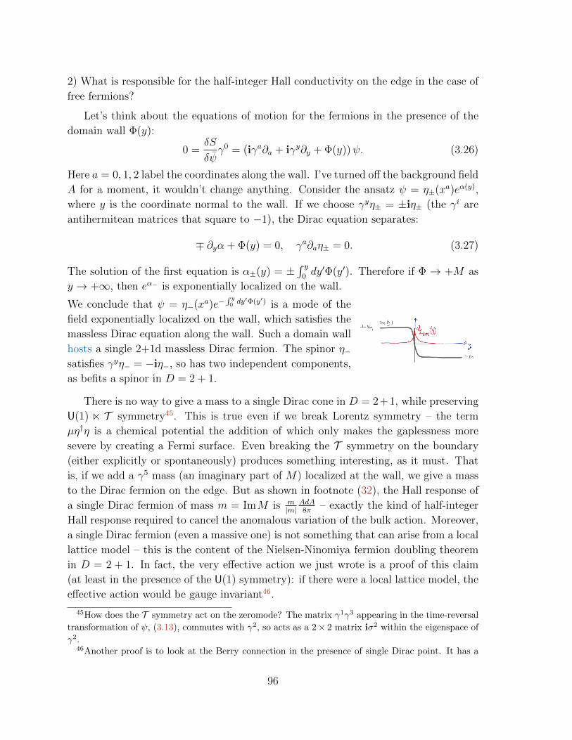
2) What is responsible for the half-integer Hall conductivity on the edge in the case of
free fermions?
Let’s think about the equations of motion for the fermions in the presence of the
domain wall Φ(y):
0 =δS
δψγ0 = (iγa∂a + iγy∂y + Φ(y))ψ. (3.26)
Here a = 0, 1, 2 label the coordinates along the wall. I’ve turned off the background field
A for a moment, it wouldn’t change anything. Consider the ansatz ψ = η±(xa)eα(y),
where y is the coordinate normal to the wall. If we choose γyη± = ±iη± (the γi are
antihermitean matrices that square to −1), the Dirac equation separates:
∓ ∂yα + Φ(y) = 0, γa∂aη± = 0. (3.27)
The solution of the first equation is α±(y) = ±∫ y
0dy′Φ(y′). Therefore if Φ → +M as
y → +∞, then eα− is exponentially localized on the wall.
We conclude that ψ = η−(xa)e−∫ y0 dy′Φ(y′) is a mode of the
field exponentially localized on the wall, which satisfies the
massless Dirac equation along the wall. Such a domain wall
hosts a single 2+1d massless Dirac fermion. The spinor η−satisfies γyη− = −iη−, so has two independent components,
as befits a spinor in D = 2 + 1.
There is no way to give a mass to a single Dirac cone in D = 2+1, while preserving
U(1) n T symmetry45. This is true even if we break Lorentz symmetry – the term
µη†η is a chemical potential the addition of which only makes the gaplessness more
severe by creating a Fermi surface. Even breaking the T symmetry on the boundary
(either explicitly or spontaneously) produces something interesting, as it must. That
is, if we add a γ5 mass (an imaginary part of M) localized at the wall, we give a mass
to the Dirac fermion on the edge. But as shown in footnote (32), the Hall response of
a single Dirac fermion of mass m = ImM is m|m|
AdA8π
– exactly the kind of half-integer
Hall response required to cancel the anomalous variation of the bulk action. Moreover,
a single Dirac fermion (even a massive one) is not something that can arise from a local
lattice model – this is the content of the Nielsen-Ninomiya fermion doubling theorem
in D = 2 + 1. In fact, the very effective action we just wrote is a proof of this claim
(at least in the presence of the U(1) symmetry): if there were a local lattice model, the
effective action would be gauge invariant46.
45How does the T symmetry act on the zeromode? The matrix γ1γ3 appearing in the time-reversal
transformation of ψ, (3.13), commutes with γ2, so acts as a 2× 2 matrix iσ2 within the eigenspace of
γ2.46Another proof is to look at the Berry connection in the presence of single Dirac point. It has a
96

The TI is protected by U(1)nT , so there is another way to gap out the single Dirac
cone, namely by adding the superconducting term
∆ηaεabηb + h.c. (3.28)
(a, b =↑, ↓ are the remaining spin indices) that breaks the U(1) symmetry. This is what
happens if we stick a superconductor on top of the TI surface. This state, naturally, has
some very interesting properties, too. One way to see them is to consider what happens
in the presence of a superconducting vortex. The answer is: Majorana zeromodes, as
we’ll see below.
You can see that the sum of the contribution from Sθ and from the Hall response
of the edge theory is gauge invariant. The ambiguity in Sθ is up to the stacking of an
integer quantum Hall state on the domain wall. This is a well-defined non-anomalous
D = 2 + 1 system that we can just paint on there.
This phenomenon of cancellation of anomalies between bulk and boundary is called
anomaly inflow. Let’s discuss some other examples of this phenomenon.
Anomaly inflow in D = 2 + 1. Let me explain the edge states of the IQHE in
the same language. Consider a Dirac fermion in D = 2 + 1 whose mass we regard as a
background (real) scalar field:
S =
∫d2+1x
(ψi /DAψ − φψψ
)+
∫AdA
8π(3.29)
In D = 2 + 1 the Dirac representation is irreducible and there is no chirality operator
γ5, so the mass (and hence φ) is real. (One subtlety here is visible in the last term:
as we’ve seen a single Dirac fermion in D = 2 + 1 is not something that we can make
with a lattice model in D = 2 + 1. So you could say that there is a second very heavy
Dirac fermion, which is responsible for the half-integer Hall response term at the end
of (3.29).)
Now consider a background configuration of φ(y) describing
a static domain wall. Again think about the limit where the
domain wall is very thin, so that everywhere with y < 0 has
constant mass −m, and everywhere with y > 0 has constant
mass +m. The Hall response is then described by
Seff[A] '∫
(1 + sign(y))1
8πAdA =
∫y>0
AdA
4π. (3.30)
We conclude that the left side is vacuum, and the right side
is an IQH state.
singularity with nontrivial Berry flux coming out of it. But in a lattice model, the Brillouin zone is
compact (a d-torus) and this flux has nowhere to go.
97

What is the gauge variation of the action (3.30), under A→ A+ dλ?
δλSeff =
∫y>0
1
4πdλ ∧ dA stokes
= −∫y=0
λεabF
ab
4π. (3.31)
This failure of gauge invariance is analogous to that of (3.25).
Again consider the Dirac equation in the presence of the domain wall:
0 =δS
δψγ0 = (iγa∂a + iγy∂y − φ(y))ψ
where now a = 0, 1. Making a similar ansatz ψ = η±(xa)eα(y), with γ01η = ±η, with
γ01 = γ0γ1, we again separate the Dirac equation. We find a chiral fermion mode
iγa∂aη = 0, γ01η = η. (3.32)
Note that γ01 is the 2d chirality operator, the analog of γ5 along the string worldsheet.
If we couple this system to the background gauge field A, a charged chiral fermion
mode produces a 2d version of the chiral anomaly:
δλS2d[A] =
∫y=0
λ∂µjµ =
∫y=0
λεabF
ab
4π(3.33)
(this is half the value you’ll see quoted for the chiral anomaly of a 2d Dirac fermion;
that’s because we have only the right-mover). This variation cancels the bulk contri-
bution (3.31). In this case, there is no option of gapping out the edge mode.
Anomaly inflow in codimension two. Let’s return to the D = 3 + 1 axion
electrodynamics (3.20) related to the 3+1d TI. Now recall that π1(V = S1) = Z for
this system, so there are topologically-protected vortex string defects. Since Φ, when
real, is a proxy for the TI bandstructure, maybe you won’t be too surprised that
something like the physics below occurs on dislocation lines in a TI47.
In cylindrical coordinates, where ρ is the distance from the
string, such a vortex string has a profile like Φ = f(ρ)eiϕ,
where f(ρ→ 0)→ 0, f(ρ→∞)→M . What we have to say
is insensitive to the detailed form of f , which looks roughly
like the figure at right.
47Actually, what happens on a dislocation line is a helical mode: a pair of complex fermion modes
with opposite chirality. Since, as we saw above, a dislocation line can be regarded as a dipolar
boundstate of disclination lines, this strongly suggests that a disclination line in a TI should carry a
chiral mode like we are seeing here. I’m not sure if this has been studied.
98

Now apply an electric field along the string, ~E = Ez. According to (3.22), this
produces a current flowing radially in to the string,
~J = − e
4π2Eρ
ρ. (3.34)
The divergence of this current satisfies ~∇ · ~J = 0 for ρ 6= 0, but∫R
~∇ · ~J stokes=
∮∂R
d~n · ~J =
∫ 2π
0
dϕρJρ = −eE2π.
But charge conservation then requires that the charge has to go somewhere – the string
acquires charge, and the charge per unit length accumulating on the string (per unit
time) is:dQ
dt= −
∫R
~∇ · ~J =eE
2π. (3.35)
We conclude
∂µJµ = δ2(x⊥)1
4πεabFab (3.36)
where x⊥ are the two directions transverse to the vortex.
(Cliff-hanger!) [End of Lecture 16]
I claim that the resolution is that the string has a normalizable charged chiral
fermion zeromode. That is, the Dirac field has a mode which instead of being a plane
wave like in empty space is exponentially localized on the vortex, and satisfies the 2d
chiral Dirac equation. But now think about the world from the point of view of the
worldsheet of the string. It is a QFT in D = 1 + 1 with a chiral fermion, like the edge
of an integer QH state, and this chiral fermion carries charge under the gauge field A.
But then the chiral anomaly in D = 1 + 1 implies that the 2d chiral current is violated
by a definite amount in a background EM field:
∂aja =1
4πεabFab (3.37)
where a = 0, 1 labels coordinates along the string, and j is the current restricted to the
string worldsheet at x⊥ = 0. This violation of charge conservation exactly accounts
for the violation of charge conservation by (3.36). (Notice how tightly constrained
everything was! Even I could get the factors of two right eventually.)
So this is an example where the anomaly of an ‘edge theory’ is cancelled by a bulk
theory with two more dimensions.
Let me outline the discovery of the zeromode in this case. The Dirac equation in
the vortex background, assuming azimuthal symmetry, isiγa∂a + iγ2
cosϕ+ iγ23 sinϕ︸ ︷︷ ︸=eiγ23ϕ
∂ρ
ψ∓ = f(ρ)e±iϕψ±. (3.38)
99

Here we’ve decomposed γ5 = γ01γ23, with γ01 ≡ −γ0γ1, γ23 = iγ2γ3 are respectively the
chirality operators along and transverse to the string, and we’ve written the equation
in a chiral basis where γ5ψ± = ±ψ±. The weird second term just comes from the
derivative terms normal to the string. Note that we’ve ignored the possibility of a
gauge field profile as a result of the vortex. Such a profile can lower the energy of the
vortex. But the zeromode will exist either way – we can absorb the gauge field bits into
a field redefinition of ψ, so let’s just ignore it. In fact, the existence of this zeromode
is guaranteed by an index theorem (this version is due to Callias), relating the number
of zeromodes of the Dirac operator to integrals of curvatures.
This equation (3.38) is solved by
ψ+ = −iγ2ψ−, ψ− = η(xa)e−∫ ρ0 f(ρ′)dρ′ (3.39)
if
iγa∂aη = 0, γ01η = −η. (3.40)
This last condition (3.40) is exactly the 2d Dirac equation for a chiral fermion. Restor-
ing the coupling to A, because ψ is charged under A, so is η coupled to A(x⊥ = 0).
Using the form of the 2d chiral anomaly (3.33), we conclude that
δλ (Sbulk + Sstring) =
∫Σ
λ∂µJµ +
∫Σ
λεαβF
αβ
4π= 0, (3.41)
where Σ is the 2d worldsheet of the string.
100
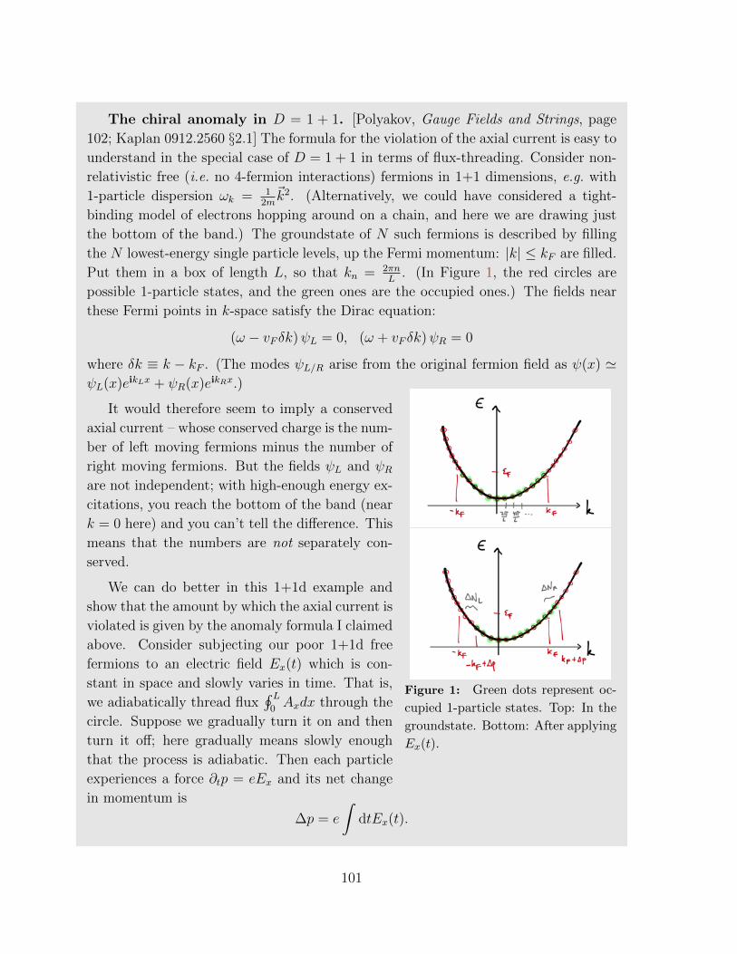
The chiral anomaly in D = 1 + 1. [Polyakov, Gauge Fields and Strings, page
102; Kaplan 0912.2560 §2.1] The formula for the violation of the axial current is easy to
understand in the special case of D = 1 + 1 in terms of flux-threading. Consider non-
relativistic free (i.e. no 4-fermion interactions) fermions in 1+1 dimensions, e.g. with
1-particle dispersion ωk = 12m~k2. (Alternatively, we could have considered a tight-
binding model of electrons hopping around on a chain, and here we are drawing just
the bottom of the band.) The groundstate of N such fermions is described by filling
the N lowest-energy single particle levels, up the Fermi momentum: |k| ≤ kF are filled.
Put them in a box of length L, so that kn = 2πnL
. (In Figure 1, the red circles are
possible 1-particle states, and the green ones are the occupied ones.) The fields near
these Fermi points in k-space satisfy the Dirac equation:
(ω − vF δk)ψL = 0, (ω + vF δk)ψR = 0
where δk ≡ k − kF . (The modes ψL/R arise from the original fermion field as ψ(x) 'ψL(x)eikLx + ψR(x)eikRx.)
Figure 1: Green dots represent oc-
cupied 1-particle states. Top: In the
groundstate. Bottom: After applying
Ex(t).
It would therefore seem to imply a conserved
axial current – whose conserved charge is the num-
ber of left moving fermions minus the number of
right moving fermions. But the fields ψL and ψRare not independent; with high-enough energy ex-
citations, you reach the bottom of the band (near
k = 0 here) and you can’t tell the difference. This
means that the numbers are not separately con-
served.
We can do better in this 1+1d example and
show that the amount by which the axial current is
violated is given by the anomaly formula I claimed
above. Consider subjecting our poor 1+1d free
fermions to an electric field Ex(t) which is con-
stant in space and slowly varies in time. That is,
we adiabatically thread flux∮ L
0Axdx through the
circle. Suppose we gradually turn it on and then
turn it off; here gradually means slowly enough
that the process is adiabatic. Then each particle
experiences a force ∂tp = eEx and its net change
in momentum is
∆p = e
∫dtEx(t).
101

This means that the electric field puts the fermions in a state where the Fermi surface
k = kF has shifted to the right by ∆p, as in the figure. Notice that the total number
of fermions is of course the same – charge is conserved.
Now consider the point of view of the low-energy theory at the Fermi points. This
theory has the action
S[ψ] =
∫dxdtψ (iγµ∂µ)ψ ,
where γµ are 2 × 2 and the upper/lower component of ψ creates fermions near the
left/right Fermi point. In the process above, we have added NR right-moving particles
and taken away NL left-moving particles, that is added NL left-moving holes (aka anti-
particles). The axial charge of the state has changed by
∆QA = ∆(NL−NR) = 2∆p
2π/L=L
π∆p =
L
πe
∫dtEx(t) =
e
π
∫dtdxEx =
e
2π
∫εµνF
µν
On the other hand, the LHS is ∆QA =∫∂µJAµ . We can infer a local version of this
equation by letting E vary slowly in space as well, and we conclude that
∂µJµA =
e
2πεµνF
µν .
If we had only the right-moving fermion (impossible in a D = 1 + 1 lattice model),
the anomaly would be half as big.
WZ descent. Let’s formalize a little bit the cancellation of the anomaly in terms
of what is called the Wess-Zumino descent procedure that relates anomalies in various
dimensions. The cancellation follows from the relations
ID+2 = dI(0)D+1, δID+1 = dI
(1)D .
Here Ik is a k-form. δ indicates gauge variation, and d is exterior derivative. In the
above, we have D = 2,
I4 =F ∧ F
8π2, I
(0)3 =
A ∧ F8π2
, I(1)2 =
λ
2π
F
4π.
The axion electrodynamics action (3.20) contains the interesting term
Sθ =
∫M4
θI4IBP= −
∫M4
dθ ∧ I(0)3
if ∂M4 = 0. Then its gauge variation is
δ
(−∫M4
dθ ∧ I(0)3
)= −
∫M4
dθ ∧ δI(0)3 = −
∫M4
dθ ∧ dI(1)2 =
∫M4
d2θ ∧ I(1)2 .
102

Now the axion winds around the string, so∮around string
dθ = ∆θ = 2π =
∫disc around string
d2θ
so we can approximate d2θ = 2πδ2(Σ), where Σ is the string worldsheet. Therefore
δλSθ = 2π
∫Σ
I(1)2
which is the formula for the 2d anomaly.
The reason to go through this trouble of formalizing is twofold: first, the same story
relates local anomalies in any even dimensions D and D+ 2. Second, it’s now easy for
me to say what happens if we redo this in a fixed curved spacetime background: we
just add some terms to the Is that depend on the curvature:
I4 =F ∧ F
8π2− trR ∧R
48 · (2π)2.
I(0)3 and I2 then get extra terms involving the gravitational CS term and R respectively.
In fact in every even dimension, these objects are all pieces of the same thing:
I = A(TM) ∧ treF2π .
This is a formal sum of differential forms of different (even) degree; the chiral anomaly
in D dimensions, ID, is the D-form piece of it. A(TM) is called the A-roof genus and
is a polynomial in the curvature form. The quantity I is the integrand of the RHS of
the Atiyah-Singer index theorem counting zeromodes of the Dirac operator. As we’ll
see below, this is not an accident.
Zeromodes on vortices. Essentially the same calculation shows that a vortex of
a p + ip superconductor carries a majorana zeromode. This is the basic mechanism
by which the Moore-Read state (or any other realization) exhibits Ising topological
order. But let’s consider a vortex in the Fu-Kane superconductor on the surface of
a TI, preserving ZT2 but breaking the U(1) symmetry. The action for the edge Dirac
mode is
S[η,∆] =
∫d2+1x (ηiγµDµη + ∆ηaiεabηb + ∆?η?aiεabη
?b ) . (3.42)
a, b are (2+1)d spinor indices. You can check that this action is real. Here we regard the
superconducting pairing function ∆ in the same way we regarded the background field
Φ earlier. We allow it to depend on space, for example in a vortex configuration,
∆ = eiϕf(ρ). Just to be clear: this is a continuum description of a vortex in a
superconductor stuck to the surface of a TI.
103

So the Dirac equation is
0 =δS
δηγ0 = iγµDµη −∆?σ2η? (3.43)
Let’s choose the gamma matrices to be γ1 = σ2 = iε, γ2 = σ3, γ0 = iσ1 (mostly
plus convention); this choice can’t matter. If we look for solutions independent of the
azimuthal coordinate ϕ, we haveiγ0∂t + iγ1(cosϕ+ iγ12 sinϕ
)︸ ︷︷ ︸=eiγ12ϕ
∂ρ
η = ∆?γ1η? (3.44)
where γ12 = iγ1γ2 is the chirality operator in the two space directions. Now let’s look
for a solution independent of t (a zeromode). Choosing γ12η± = ±η±, we have
e±iϕi∂ρη± = f(ρ)e−iϕη?± . (3.45)
To match the ϕ-dependence, there can only be a solution for η−.
A crucial point: (3.45) is not a linear equation in η over the complex numbers. It
determines the phase of η. Make the ansatz η− = eiαη0 for some real chiral spinor η0.
Then we have
ei(π2
+2α)∂ρη0 = f(ρ)η0.
To have a normalizable real solution
η0(ρ) = e−∫ ρ0 dρ
′f(ρ′),
this equation must take the form ∂ρη0 = −f(ρ)η0, which means
π
2+ 2α
!= π
meaning that α = π4.
The particular answer for the phase is not important and would change if we
changed representation of gamma matrices, but the point is that the phase is fixed:
we have found a majorana zeromode. This is a fermion zeromode satisfying a reality
condition. The mode expansion of the quantum field η(xµ) is then something like
η(xµ) = eiαη0(ρ)γ +∑k
(aku
+k (x) + b†ku
−k (x)
)(3.46)
where the second term is the usual thing with operators that create and annihilate
particles and antiparticles in states that look like plane waves far from the vortex,
104

u±k (x) ∼ e±ikµxµ
for large |x|. Canonical commutation relations then tell us that the
mode operator γ anticommutes with the other modes and squares to 1.
What’s the big deal? Suppose we put N well-separated vortices. Then each vor-
tex A = 1..N will have its own real zeromode (that they are exponentially localized
guarantees that they are exponentially close to being zeromodes48), ηA0 , and associated
majorana zeromode operator γA. They anticommute with all the other mode operators
(and hence the Hamiltonian) and amongst themselves satisfy the (Clifford) algebra
γA, γB = δAB. (3.47)
What are the representations of this algebra? For N zeromodes there are 2bN2c states
(where bxc denotes the floor of x, the largest integer smaller than x). This grows like√2N
at large N . It is as if there are√
2 states per vortex. The Hilbert space therefore
cannot be stored locally on the vortices. The operations of adiabatically moving the
(identical) vortices around each other and exchanging them act on the Hilbert space
by interesting unitary operators – it gives a representation of the (infinite) braid group
on N elements that is not just a representation of the (finite) permutation group, SN .
In the Fu-Kane superconductor (and in a p + ip superconductor), the objects car-
rying the majorana zeromodes are extrinsic defects rather than dynamical particle
excitations of the system. This system does not have non-abelian topological order.
The situation is different in the Moore-Read state, and in another surface termination
of the TI that we’ll construct momentarily.
More about the Witten effect. Consider a ball of TI.
When we bring a magnetic monopole from the vacuum out-
side into the TI, it acquires electric charge e/2. (The charge
is ambiguous modulo e, because an electron or hole can stick
to it.) Charge conservation then requires that a compensat-
ing charge −e/2 is stuck to the boundary of the TI somehow.
Each of the many possible boundary conditions accomplishes
this in its own way, and it’s worth examining these mecha-
nisms.
The simplest is the Fu-Kane superconductor, ∆L = ησ2η + h.c.: a superconductor
breaks the U(1) symmetry and can absorb arbitrary amounts of charge. End of story.
48Assuming an extra discrete symmetry, the Callias index theorem guarantees that they are exact
zeromodes. See Appendix B of this paper.
105

Next simplest is a time-reversal-breaking surface, ∆L = mηη. We saw already how
moving a monopole through the surface is consistent with global charge conservation
because of the two terms in the contribution to the electric charge density ρ from the
theta term, (3.22) – the surface carries charge e/2 in the presence of 2π flux. Actually
we knew this from the Laughlin flux-threading argument: threading localized 2π flux
through a system with Hall conductivity σxy = ν e2
hproduces a quasparticle with charge
eν, which here is ±12
depending on the way in which we break time reversal. This
charge then gets transported around the surface by the Hall effect due to the moving
monopole.
What happens when there is a gapless edge? Think about the case where the
boundary of the TI is a nice round S2. In that case, the Dirac field η on the surface
is living on an S2 with a single magnetic monopole inside. This is a classic problem.
The answer is that η has zeromodes. These are eigenvectors of the Dirac operator
on S2 with one unit of flux∮S2 F = 2π, with eigenvalue zero. Their number is the
subject of the Atiyah-Singer index theorem, which says that the number of right-
handed zeromodes minus the number of left-handed zeromodes of the Dirac operator
on an even-dimensional manifold X is
n+ − n− =
∫X
A(TX) ∧ treF2π
X=S2
=
∫S2
F
2π= 1. (3.48)
This quantity is topological because nonzero eigenvalues of D ≡ iγµDµ come in pairs
related by the action of the chirality operator. That is, nonzero-energy eigenstates of
H ≡ D,D† are all doubly-degenerate, with one state of each chirality. This means
small deformations of D can only change the number of zeromodes by the addition
or subtraction of one of each chirality. The statement (3.48) is some pretty heavy
machinery, but for physics purposes it essentially follows from the QFT derivation of
the chiral anomaly.
What is the consequence of the single zeromode η0 of η guaranteed by the index?
Unlike in the Fu-Kane discussion, this Dirac equation is linear, so this is a complex
zeromode, which carries U(1) charge 1. It leads to a complex fermion zeromode operator
c† of charge 1 (η(x) = η0c+nonzeromodes), satisfying c, c† = 1 (and commuting with
all the other nonzeromode operators, and the Hamiltonian). This means that there are
two degenerate states |−〉 annihilated by c and |+〉 = c† |−〉 annihilated by c†. These
two states have electric charges q± that differ by 1 (or e): q+ − q− = 1, and they are
related by charge conjugation symmetry, so q− = −q+. We conclude that these two
states have charge ± e2. After the monopole enters the TI, the charge is spread out all
over the surface according to the wavefunction η0 of this zeromode.
Finally, there is another possibility for a surface state of the TI: there can be
a gapped, symmetric surface. Think about what happens when a monopole enters
106

a TI with such a surface. In such a gapped state, charge cannot propagate freely.
The charge e/2 that gets stuck on the surface when the monopole enters must be
carried by a gapped quasiparticle with charge −e/2. We conclude that the gapped
symmetric surface must be fractionalized, i.e. must have topological order, since it
hosts a quasiparticle of fractional charge. Next we turn to a simple way to describe
such a state. 49
Symmetric gapped surface of D = 3 + 1 TI. Here is a way to motivate the
D = 2 + 1 topological order that carries the same anomaly as a single Dirac cone,
or as the Fu-Kane superconductor, or as the state with 12-integer Hall response. Such
states were first constructed in these four papers, and later understood better using
D = 2 + 1 dualities in these papers. There is also a close relation with Son’s particle-
hole-symmetric description of the half-filled Landau level. The construction I’ll describe
comes from here.
Begin with the single Dirac cone
S[η] =
∫d2+1xηiγµDµη. (3.49)
Let’s regard this as the Higgs phase of some new U(1) gauge theory. Essentially, we
are making a parton construction, with ansatz
η = χwn . (3.50)
The charge assignments are:χ φ w
A 1 2 0
a n 2n −1
(3.51)
Here χ is a Dirac fermion with a kinetic term just like (3.49), and φ and w are complex
scalar fields, with appropriate kinetic terms. n is a number that we’ll fix below.
First, to see why we should care about this theory, observe that if we condense w
(but not φ), we Higgs the new U(1), and we can forget about it, and we are back to
49There is another, unphysical, possibility for the surface that sometimes occurs in solvable lattice
models, called symmetry extension. That is, the protecting symmetry group G could be a subgroup
of a larger symmetry H ⊃ G in the presence of an edge, with the property that the anomaly for G
is not an anomaly for H. Certainly it’s possible for the edge theory to have some enlarged emergent
symmetry. But this is unphysical because it requires H to be an exact symmetry of the theory with a
boundary, since G ⊂ H. In contrast, emergent symmetries are always broken by irrelevant operators.
I recommend this talk by Witten for a clear discussion of an example where this happens.
Such a solvable model can be used to construct a gapped symmetric boundary state, by gauging
H/G. In that case, the would-be extra symmetry is just a redundancy of description – certainly H/G
gauge theory is allowed to emerge.
107

the theory of η, (3.49), since if w is condensed then (3.50) says η = χ 〈wn〉 = χ. This
already proves that the two theories have the same anomalies, whatever other phases
they realize.
[End of Lecture 17]
The role of φ is more interesting. We should think of φ as arising by decoupling a
four-fermion interaction of χ in the s-wave BCS channel. This just means that with
the given charge assignments, we can (and should) add a term that looks a lot like the
Fu-Kane term, an s-wave pairing term for χ:
Lφ = φχaiεabχb + h.c. (3.52)
where the dynamical field φ plays the role of the superconducting pair field ∆. But
now think about what happens in a phase where we condense φ (but not w): since φ
is charged under both a and A, condensing φ higgses a combination of them down to
a diagonal subgroup, which we can regard as the new global U(1) symmetry to which
A is coupled. (The mass term is (2A + 2na)2; varying a will just set a = −2A/2n,
and there is no mass term for A.) The global U(1) that survives is the subgroup under
which φ is neutral, with generator q = qA− qa/n. The effective table of charges in this
phase is then:χ φ w
A 0 0 −1/n(3.53)
Moreover, since φ carries charge 2n > 1 under U(1)a, a discrete (Z2n) subgroup of U(1)asurvives. This is a gapped state with topological order that preserves the protecting
symmetry G = U(1) n ZT2 , so it must be interesting somehow.
Ignoring the fermions, this would just be Z2n gauge theory, an abelian topological
order. But now let’s think about the vortices of φ. These are actual dynamical quasi-
particles in the system. A vortex of φ has fractional flux∫
f2π
= 12n
– it is an m-particle
or ‘vison’ of the Z2n topological order. Ignoring the fermions, the quasiparticles would
be labelled by e and m quantum numbers (k, v) and would satisfy the abelian braiding
statistics WkvWk′v′ = Wk′v′Wkve2πi(kv′−k′v)
2n .
But the Dirac equation for χ is just the same as in our discussion of the Fu-Kane
superconductor. We conclude that the vortex carries a majorana zeromode. There is
a crucial physical difference, however: in the Fu-Kane case, the vortex was an external
defect of a fixed background field ∆. In contrast, φ is a dynamical variable on the
surface of the TI – its vortices are quasiparticles. (And they have finite energy, since
the U(1) acting on the phase of φ is gauged.)
You could ask about charge v > 1 vortices, which seem to have v majorana zero-
modes γi. But in the absence of extra discrete symmetries, nothing forbids quadratic
108

terms iγiγj in the Hamiltonian which lift these zeromodes. So odd v vortices have a
single majorana zeromode, and even v vortices have none.
So far we have not determined n. Let us think about the monopole operators of
this U(1) gauge theory. A monopole operator is a kind of disorder operator, defined
by a boundary condition in the path integral over a. The monopole operator eiσ(x)
is defined by cutting out a small ball around the spacetime point x, and demanding
that on the boundary S2x of this ball, we have
∮S2xf = 2π, as if there were a magnetic
monopole inside: ⟨eiσ(x) · · ·
⟩≡ Z−1
∫∮S2xf=2π
[Da]eiS · · · . (3.54)
The quantum numbers of such an operator can be determined by regarding the radial
direction away from the point x as time, so that the S2 surrounding x is an equal-time
slice. The quantum numbers of the operator are just those of the resulting groundstate
on S2 with flux50.
The Dirac field χ has charge n, and so the same index theorem we used above
predicts that it has n complex chiral zeromodes on S2 with one unit of flux, whose
associated operators we’ll call χi=1..n. Being a mode of a spin-half field, each χi has
half-integer spin. They satisfy
χi, χ†j = δij, χi, χj = 0 = χ†i , χ†j.
This algebra is represented by starting with a lowest-weight state |⇓〉 annihilated by
all the χis, and acting with χ†is until we get to a highest-weight state |⇑〉, annihilated
by all the χ†is. Let’s determine the U(1)A × U(1)a charges and spins of these states:
each χ†i adds charge ∆q = (−1,−n), and a half unit of spin. The spectrum of charges
must be symmetric about zero, so we must have
q⇑ = −q⇓ = q⇓ + n∆q
from which we conclude that the charge of |⇓〉 is q⇓ =(n2,−n2
2
). The states in the
middle
χ†i1 · · ·χ†in/2|⇓〉 (3.55)
have charge(n2,−n2
2
)+ n
2(−1,−n) = 0.
Now we can constrain n on physical grounds. First, if n is odd, the spectrum
cannot be symmetric under charge conjugation. For example, if n = 1, the states
50More precisely, this statement uses the state-operator correspondence of conformal field theory.
Conformal symmetry is valid at high energies in the system we are studying, and so we can use it to
determine the microscopic quantum numbers of the monopole operators here.
109

|⇓〉 and |⇑〉 = χ†1 |⇓〉 have spins differing by a half-integer, and therefore cannot be
related by a discrete symmetry. So we assume n = 2s is even. This means that there
are gauge-invariant local monopole operators associated with the states (3.55). These
states have integer or half-integer spin according to whether s is even or odd51, i.e. the
associated gauge-invariant monopole operator eiσ(x) has spin s/2 mod Z, and is neutral
under U(1)A. But in a condensed matter system with all the degrees of freedom made
from electrons, all half-integer-spin particles (fermions) carry odd charge under U(1)A.
There is no way even the magic of emergence can change this property, it’s a property
of the Hilbert space. This ‘spin-charge relation’ is only satisfied by this gauge theory
if s is even. We conclude that the minimal possible value of n is n = 2s = 4.
Being more explicit about the potential terms, we
can write
Lr = uw|w|4 + rw|w|2 + uφ|φ|4 + rφ|φ|2 (3.56)
and we can think about varying the signs of rw, rφto condense or not each of w, φ. The phase diagram
looks schematically like the figure at right. The walls
are surface phase transitions, leaving the bulk SPT
intact.
The upper right corner, where neither φ nor w is condensed is less easy to un-
derstand. Presumably the U(1) gauge theory confines by the Polyakov mechanism,
because it has only a single Dirac fermion charged under it (I think the current consen-
sus is that the critical number of flavors above which U(1) gauge theory in D = 2+1 is
deconfined is Nf = 2). Does the fact that χ has charge 4 make a difference? Maybe. So
we should look for gauge-invariant objects. The gauge invariant fermionic boundstate
χwn is then the right degree of freedom to consider. (Are there others? There are also
monopole operators, the bosonic ones of which should be added to the action52.) But
this is just η, and it can’t get a mass unless we break T or U(1). So maybe this is just
the same phase as the upper left.
Exercises:
1. Apply the same technique to identify topologically-ordered symmetric gapped
edge states for the case where the bulk is protected by G = U(1)×Z2 nZ2 where
51Here I appeal to the fact that |⇓〉 is a unique state annihilated by all the χi, which therefore must
have spin 0.52Note that these operators should also be added to the action in the phases with 〈φ〉 6= 0. But there
they don’t do much besides explicitly break the flux conservation symmetry which is not a microscopic
symmetry.
110

the extra Z2 is a chiral particle-hole symmetry as in this paper. The consequence
of this extra symmetry is that an arbitrary integer number k of Dirac cones on
the surface is protected – the classification is Z rather than Z2.
2. Apply the same technique to understand the edge states of a D = 3+1 topological
superconductor, like 3 He-B.
3.3 Coupled-layer construction
The simplifying assumptions defining SPT states allow them to be built from lower-
dimensional parts, actually in several different ways. (So it is a good idea to understand
low-dimensional examples well.)
The idea of this subsection comes under many names. It is sometimes called the
coupled-layer construction, or network construction, of SPTs.
The idea is to start with just the edge theory E and its inverse E in D−1
dimensions. This is what we would have if we had a very thin slab of the
SPT. Call this a layer. Since E by definition has the opposite anomaly
to E, a layer has no anomaly, and can be realized symmetrically in D− 1
dimensions.
Now take a bunch of layers and make a one-dimensional chain of them. This makes
a trivial state in D dimensions. But in this chain, each E is next to the E from the
next layer, and there is a natural coupling between them. If we make this coupling
larger than the one within the layer, we can drive a transition to a new D dimensional
state that manifestly has E at one end and E at the other, which is the SPT.
Here are many examples.
• AKLT/Haldane chain. An example of an edge for a D = 1 + 1 SPT for
G = SO(3) is a single spin-12. A pair of spin-1
2s is a linear representation of
SO(3), not a projective representation, since the two signs in the 2π rotation
cancel out. Call this a layer and label the two spin operators ~S and ~S. It can be
destroyed by the symmetric hamiltonian
H0 =∑i
~Si · ~Si (3.57)
within the layer. We can depict the groundstate of H0 as at right, where each
small circle represents a spin one-half, and the blobs represent singlets. (This
system is in the same phase as the spin-1 Heisenberg model; the difference is just
the singlet in 2⊗ 2 = 1⊕ 3, which plays no role.)
111

Now there are naturally two distinct ways of gapping out the bulk. One is with
H0, and the other is with the pairing
Hg = gN−1∑i=1
~Si · ~Si+1 (3.58)
between the right spin of one layer and the left spin of the next. When g 1 we
are in a gapped phase distinguished from the trivial one by the fact that the left
spin-12
of first layer and the right spin-12
of the last are unpaired, as depicted in
(3.58) for the extreme limit, where the wavefunction takes the form
|AKLT〉 = ⊗i∣∣∣↑i ↓i+1 −↓i ↑i+1
⟩/√
2. (3.59)
The edges of the chain thus lie in projective representations of the symmetry group
SO(3). This is the general property of the edge states of SPTs in D = 1 + 1. One
is led to believe, then, that they are classified by the group cohomology group
H2(G,U(1)) that classifies projective representations of G.
Notice that there must be a phase transition at some point in between as we
increase g. It happens when g = 1, so that we get a homogeneous spin-half
Heisenberg chain. This model is described at low energies by the SU(2)1 WZW
model CFT with cL = cR = 1. The model is also exactly solvable by Bethe
ansatz.
A very similar story obtains with the same degrees of freedom if instead of SO(3),
we choose the protecting symmetry to be G = ZT2 , time-reversal symmetry.
Recall Kramers’ theorem: on a spin-half, T 2 = −1. Such a pair of states is called
a Kramers’ doublet, whose degeneracy can’t be split while preserving T 53. On
a pair of spin-halfs, in contrast, T 2 = 1. So if we make a 1d array of an even
number Kramers’ doublets, we again have two choices for how to pair them (for
example by the Heisenberg interaction), and the interesting one leaves behind a
single Kramers’ doublet at each end. Notice that this is a Z2 classification, since
a pair of such doublets can be destroyed by the symmetric hamiltonian (3.58) (or
just XX + ZZ).
• Kitaev chain. Consider a single complex fermion mode c in 0 + 1 dimensions,
with c, c† = 1. Regard this as two majorana modes c = γ+iγ√2
, with γ, γ =
53Here is the proof that |ψ〉 and T |ψ〉 are orthogonal when T 2 = 1:
〈ψ| T |ψ〉 antiunitary= (〈T ψ|ψ〉)? antiunitary
= T 〈T ψ|ψ〉 =⟨T 2ψ|T ψ
⟩ T 2=−1= −〈ψ|T ψ〉 = 0.
I learned this argument from Yi Li.
112

0, γ2 = 1, γ2 = 1, and think of γ and γ as generating the edge states E and E
respectively.
To specify what I’m talking about, I should say what is the protecting symmetry
I have in mind. Let’s consider two cases: G = ZT2 and no symmetry. ZT2 acts by
c→ c, i→ −i, so γ → γ, γ → −γ. In either case, we can add
H0 =∑i
c†ici = iγiγi (3.60)
in each layer, which has a unique groundstate (ci |0〉 = 0). We can depict the
groundstate of H0 as at right, where now each small circle represents a majorana
mode, and the blobs represent complex fermion modes whose number operator
appears in H0.
The chain of layers is then just a 1d chain of spinless fermions. With either choice
of symmetry, we can add both fermion hopping terms, as well as p-wave pairing
terms cici+1. Let’s consider the coupling
Hg = gN−1∑i=1
iγiγi+1. (3.61)
For g < 1, the gap stays open and we remain in the trivial phase. When g = 1,
the gap closes, and we have a translation-invariant majorana chain with half the
unit cell. A massless D = 1 + 1 (non-chiral) majorana fermion propagates along
the chain. (For a derivation of this statement see p. 54 here.) This is locally the
same as the critical Ising model, a CFT with c = 12. For g > 1, locally it looks
the same as the trivial phase, in that each majorana in the bulk is paired with
a neighbor. But now it is the neighbor from the next layer. This leaves out one
majorana from the first layer and one from the last as unkillable edge modes.
The extreme limit g 1 is depicted in (3.61). This is the Kitaev chain (reviewed
here). Since the two unpaired majorana modes are separated by a distance of
order system size, the product a protected qubit with degeneracy exponentially
small in the system size.
In H0 + Hg, we’ve chosen some special couplings, but the gapped phase we’ve
discovered occupies an open set in the space of all couplings of a p-wave super-
conductor of spinless electrons in 1d.
The difference between the two symmetry choices arises when we consider stack-
ing multiple copies of the Kitaev chain. If we have no symmetry, then when we
stack a pair of these chains, nothing prevents us from pairing up the two end
majoranas at each end. There is a Z2 classification in this case.
113

With the ZT2 symmetry acting as above, the coupling iγ(1)1 γ
(2)1 (where the index
in parentheses labels which chain the mode comes from) or iγ(1)N γ
(2)N is forbidden.
This suggests that an arbitrary number of chains produces an arbitrary number
of majorana modes which can’t be destroyed by adding mass terms, leading to a
Z classification.
This is true for free fermions. However, Kitaev and Fidkowski showed that al-
lowing interactions reduces this to a Z8 classification. They explicitly identify a
4-fermion term W that can lift the degeneracy of 8 majorana modes in a ZT2 -
invariant way, i.e. it has a unique groundstate.Adding this term in the bulk provides a route to go around the phase
transition of the free fermion theory that would separate k chains and
k + 8n chains. Their construction involves some lovely group theory,
featuring the triality symmetry of SO(8).
[End of Lecture 18]
• Integer quantum Hall states. Now an example where layers of D = 1 + 1
systems produce a gapped state in D = 2 + 1. To make the fermion IQHE, a
layer is just a single non-chiral boson mode φ, where the right-mover is E and
the left-mover is E. These can be gapped out by the backscattering interaction∑i t0 cosφi =
∑i t0 cos (φiL + φiR). But if we add∑
i
te cos(φiR + φi+1
L
)we can gap out all the modes in the bulk in a different way, leaving behind a
leftmover at one end and a rightmover at the other.
Alternatively, here is a model of a transition in a system of (spin-polarized)
electrons across which the Hall conductance changes by e2
h, just in terms of free
fermions.
S =
∫dxdτ
2N∑j=1
Lj
Lj = c†j (∂τ − isj∂x) cj︸ ︷︷ ︸IQHE edge
− tj(c†j+1cj + c†jcj+1
)︸ ︷︷ ︸
interlayer hopping
tj =
te, j even
to, j odd, sj = −(−1)j .
For each j we have one chiral mode, that is, a D = 1 + 1 complex chiral fermion.
The tj term is some back-scattering by which these layers hybridize and eat each
114

other.
For te < t0, all layers are paired and there’s nothing left; σxy = 0.
For te > t0, there are leftover chiral modes at the edges, σxy = e2
h. The transition
occurs at te = to, where we restore some extra translation symmetry. Taking a
continuum limit N →∞, Na fixed we find a 2+1d Dirac fermion.
A similar example for the case of
the boson IQHE is shown in the
picture at right.
In general, the way the edge ex-
citations emerge in each of these
examples is just like in the clas-
sic picture of edge charge from po-
larization of an insulator; the role
of the polarization angle is played
by arctan(teto
), where te/o are the
couplings between the layers on the
even and odd links respectively.
• D = 3 + 1 TI, with G = U(1) n ZT2 . [From here]
Here each layer EE is two Dirac cones in D = 2 + 1. For
example, we could take the layer hamiltonian to be
H0 =∑i
∮d2kc†i (k)h0(k)ci(k), h0(k) = τx (kxσy − kyσx)
where τ acts on a ‘valley degeneracy’ labelling the two cones,
which both lie at (kx, ky) = (π, π) in this approximate de-
scription. We could add a T -invariant mass that pairs them
up, but let’s not. Note that my bandstructure is not periodic
in k, but what I’ve written is just an approximation near the
Dirac points; the important thing is that it could be made
periodic, consistently with the doubling theorem.
Now couple the layers by
Hg =N−1∑i=1
(∮d2kc†i (k)h+ci+1(k) + h.c.
), h+ ≡ τz + iτy .
The (3 + 1)d bandstructure described by H0 +Hg is a discretization of a massive
D = 3 + 1d Dirac fermion. The resulting single-particle edge hamiltonians are
hedge = ±~k×~σ, and can no longer be paired up with each other because they are
115

separated by a distance of order system size.
• G = ZT2 boson SPT in D = 3 = 1. [From here] The edge state we wish to
construct is the all-fermion toric code. This is a Z2 topological order where all
the nontrivial anyon types, e,m, ε, are fermions. This arises as U(1)4 CS theory
with K matrix equal to the Cartan matrix of SO(8). But that theory is chiral (it
has four chiral boson edge modes, c− = 4) and clearly breaks T symmetry.
But two copies of this TO is related to two copies of the ordinary toric code, by a
relabelling. Each one has six fermionic anyons and 10 bosonic anyons (including
the trivial anyon), with the same braiding data. That is certainly realizable in a
T -invariant way.
So a layer in this construction will be two copies of the ordinary toric code.
We’ll stack some number N/2 of such layers. For convenience let me label the
individual toric codes i = 1..N . Now add a bulk hamiltonian that couples the
layers and has the consequence that the objects
Bi ≡ εimi+1εi+2
condense. Bi is a boson (since it’s made of two fermions and a boson with trivial
mutual statistics), so it makes sense to condense it. Moreover, different Bi have
trivial mutual statistics, so we can condense them at the same time. (We could
just add ∆H = −∑N−2
i=1 Bi.)
In the diagram at right, for N = 6, the objects circled in red
are Bs. You can ignore the daggers on ε = ε†. Condensing
B destroys all the topological order in the bulk, since each
bulk anyon has nontrivial braiding with something in the
condensate. The nontrivial anyons that survive (circled in
yellow) are ε1 and m1ε2 at one end (and their boundstate),
and εN−1mN and εN (and their boundstate) at the other.
But these particles are all fermions!
A very similar construction produces a different SPT with the same symmetry,
where all the quasiparticles are Kramers’ doublets.
3.4 Wavefunctions for SPTs
Decorated defects. If we are interested in making paramagnetic states, one way to do
it is to begin with the ordered state, and then destroy the order by condensing defects,
116

like the ones we studied in §1. This point of view in terms of defects in the would-be-
bose-condensate turns out to be very fruitful. The completely trivial Mott insulator
of the bosons with U(1) symmetry is described in this language as a condensate of
featureless vortices (in 2+1d; in 3+1d they are vortex loops). (With Z2 symmetry, we
would talk about domain walls instead.) More interesting states are obtained instead
if the defects in the order carry some kind of decoration. A scheme for understanding
SPT states then follows by characterizing possible decorations of the defects. I will not
pursue it explicitly here.
BF theory for 3+1d boson SPTs. Consider the following D = 3 + 1 analog of
CS theory
S[B, a] =∑I
1
2πBI ∧ daI + ϑ
∑IJ
KIJ
4π2daI ∧ daJ
Note that the theta angle ϑ here is not the same as the θ in the magnetoelectric resonse,
but time-reversal symmetry requires ϑ = 0 or π.
This is called BF theory because the lagrangian is B times f . It is topological,
like CS theory, in that we didn’t need to introduce the metric to integrate the action
covariantly. In D = 3 + 1 we need the form degrees to add up 2 + 1 + 1 = 4. We can
add analogs of Maxwell terms (for both B and a), but just like in D = 2 + 1 they are
irrelevant, i.e. they merely introduce new UV physics, they don’t change the IR.
(The coefficient of the B∧f term is chosen so that there is no bulk topological order.
If we multiply it by k we get a description of Zk gauge theory. Note that the more
general seeming thing with a more general matrix coupling f and B can be removed
by an integer-valued field redefinition that changes nothing.)
Briefly, who are these variables? Focus on the case K = σx. In D = 2 + 1: the
flux of the CS gauge field was some charge density. Here, each BI implements a 3+1d
version of charge-vortex duality, where for each boson current
jI=1,2µ =
1
2πεµ···∂·B
I··
which has ∂·jI· = 0 as long as B is single-valued. The point of a is to say that B is
flat, so that there are no local bulk degrees of freedom.
One virtue of this effective action is that it reproduces the EM response we expect
of a topological insulator. If we couple to an external U(1) gauge field A by
∆L = Aµ (jµ1 + jµ2 )
then
log
∫[DaDB]eiS[a,B,A] =
∫2ϑ
8π2dA ∧ dA+ · · ·
117
that is, the magneto-electric response is θEM = 2ϑ. So ϑ = π will be a nontrivial boson
TI. You can also see from the equations of motion that the magnetic field lines of aIµare the vortex lines of the microscopic bosons bI .
Ways of slicing the path integral. Now let’s think about the path integral for a
QFT with a theta term. Examples include the BF theory above, and many non-linear
sigma models which arise by coherent-state quantization of spin systems. In general
what I mean by a theta term is a term in the action which is a total derivative, and
where the object multiplied by theta evaluates to an integer on closed manifolds. The
following point of view has been vigorously emphasized by Cenke Xu.
When spacetime is closed Z(θ + 2π) = Z(θ). On a closed spacetime manifold MD
Zθ(MD) ≡∫
[Dstuff]e−S =∑n∈Z
eiθnZn
and Zθ(MD) = Zθ+2π(MD). In particular, we can take MD = S1 × ND−1 to compute
the partition function on any spatial manifold ND−1. This means the bulk spectrum is
periodic in θ with period 2π.
With boundaries, it not so in general. A boundary in space produces edge states.
We’ve already said a lot about these.
A boundary in time in the path integral means we are computing wavefunctions.
For quantum mechanics of a single variable q(t), this is manifested in the Feynman-Kac
formula
ψ(q) =
∫q(t0)=q
∏t∈(−∞,t0)
dq(t) e−Seuclidean[q] .
For a field theory, ‘position-space wavefunction’ means a wavefunctional Ψ[φ(x)], in
|Ψ〉 =
∫[Dφ(x)]Ψ[φ(x)] |φ(x)〉
where x labels spatial positions, and |φ(x)〉 are coherent states for the field operator
φ(x). Which wavefunction? If the path integral is over a large euclidean time T before
reaching the boundary, this is a groundstate wavefunction, since the euclidean time
propagator e−TH is a (un-normalized) projector onto lowest-energy states.
Semi-philosophical digression: An important guiding concept in the study of in-
teresting gapped states is that it is the same stuff living at a spatial boundary (edge
modes) as at a temporal boundary (the wavefunction). This perspective first arose
(I think) in the context of quantum Hall states where one can write groundstate and
several-quasiparticle wavefunctions as correlation functions of certain operators in a
118

1+1d conformal field theory (CFT), which is the same CFT that arises at a spatial
edge. Why should this be true? It’s because the bulk can be described by a path
integral for a Chern-Simons gauge theory, which has a certain CFT (chiral bosons for
abelian CS theory, more generally a WZW model) living at its boundaries, wherever
they are. For a spatial boundary, it produces a copy of that CFT at the boundary
(roughly the group-valued CFT field g is related to the CS gauge field by a = g−1dg).
For a temporal boundary, the path integral expression for the wavefunctional (with
some Wilson line insertions at the positions of the electrons) takes the form
Ψ[g(x)] =
∫a(t0,x)=g−1dg
eiS[a]W [C] =
⟨∏α
Vα(xα)
⟩WZW
. (3.62)
A too-brief explanation of this rich formula: the wilson line insertion is W [C] =
trRPei∮C a where R is a representation of the gauge group G and P is path order-
ing. In (3.62), xα are the locations where the curve C intersects the fixed-t = t0surface, and Vα are some operators in the CFT the appropriate representations R of
G.
For 3+1d boson SPT states, the analogous bulk EFT is, instead of CS gauge theory,
some weird BF theory or strongly-coupled sigma model. At a spatial edge, we have
some vortex excitations in D = 2 + 1. Correspondingly, the bulk wavefunctions will
turn out to have a nice representation in a basis of states labelled by vortex loop
configurations in D = 3 + 1.
Side remark: the canonical application of this story is to the Haldane chain – a
chain where each site carries a representation of SO(3). At low energies, such chains are
described by an NLSM with a theta term. θ = 0 is trivial and gapped. θ = 2π is gapped
and trivial in the bulk but the edge states are spin 12s – a projective representation of
SO(3).
Let’s apply this picture to BF theory.
119

In contrast to the case of a closed manifold, if we compute the path integral on a
ball, with a boundary say at τ = 0, then θ does matter, not just mod 2π.
Choose aτ = 0 gauge. Since a and B are conjugate variables, the analog of position
space here is |~a(x)〉. For the same reason, we can only specify BCs on one or the other:∫~a(x,τ=0)=~a(x)
[D~a(x, τ)DB(x, τ)]e−S[~a(x,τ),B] =⟨~a(x)
∣∣∣gs⟩
(3.63)
Notice that in expressions for functionals like S[a(x, τ)] I am writing the arguments
of the function a to emphasize whether it is a function at fixed euclidean time or not.
The fact that the theta term is a total derivative
f I ∧ fJ = d(aI ∧ fJ
)≡ 8π2dw(a)
means that the euclidean action here is
S[~a(x, τ)] =
∫MD
1
4πB ∧ f + iϑ
∫∂MD
w(~a(x)).
The θ term only depends on the boundary values, and comes out of the integral in
(3.63).
The integral over BI is ∫[DB]ei
14π
∫BI∧aI = δ[f I ].
The delta functional on the RHS here sets to zero the flux of the gauge field for points
in the interior of the cylinder. After doing the integral over B, there is nothing left in
the integral and we can factorize the expression (3.63) to determine:
Ψ[~aI(x)] = exp iϑ
8π2
∫space
aI· ∂·aJ· ε···KIJ
︸ ︷︷ ︸K=σx
= iϑ(linking # of 2π magnetic flux lines)
(3.64)
What does this mean? Label configurations of a by the flux loops (i.e. the field
lines of the vector field). This wavefunction is (−1)linking number of the 1-loops and the 2-loops.
If we break the U(1)× U(1) symmetry, the flux lines of 1 and 2 will collimate (by
the Meissner effect).
Claim: in the presence of an edge, these flux lines can end. The ends of these flux
lines are fermions. (Warning: doing this right requires a framing of the flux lines –
i.e. they shouldn’t collide.) Conclusion: on the surface of this SPT state of bosons
there are fermionic vortices.
120

Figure 2: The end of the ribbon is a fermion: In the first step, we rotate the red string around
the blue one. The squiggles mean that the states associated with these configurations have the same
amplitude in the groundstate, according to (3.64).
Note that the BF theory describes a very strongly confined abelian gauge theory in
the following sense: the flux gets set to zero by the B term. (With a string source for
B the flux gets localized to the source.)
Comment on Kodama state of gravity. This wavefunction (3.64) actually
solves the Schrodinger equation for quantum Maxwell theory at finite coupling. There
is even a non-Abelian version of it for which this is also true. There is even an analog
for gravity called the ‘Kodama state’ ! What’s the catch? It’s not normalizable as a
wavefunction for photon fields; attempting to quantize the model about this ground-
state gives negative energy for one of the two circular polarization states. But as a
wavefunction for the confining phase of the gauge theory it’s fine.
Note that this paper does an analogous thing for very strongly coupled sigma models
with theta terms; they just set the kinetic term to zero (!) and find wavefunctions
closely analogous to (3.64). They would have the same problem as Witten points out
if they thought of their wavefunctions as wavefunctions for gapless magnons. But for
the disordered phase of the sigma model (gapped and analogous to confinement) it is
just fine. Some of these are the same wavefunctions we’ll arrive at in the following
discussion.
121

Group cohomology SPTs. Here is a nice construction of a large class of bosonic
SPTs.
To begin, suppose that spacetime is chopped up into a simplicial complex. This
means that it is divided up into volumes, each of which is a D-simplex, and each of the
faces is a D − 1-simplex and so on. We will construct a path integral. The degrees of
freedom are elements of G living on the 0-simplices (vertices). It will have the following
properties:
1. It is G-symmetric.
2. The amplitude for any configuration e−S(g) = 1 on a closed spacetime manifold.
3. The amplitude e−S(g) is subdivision invariant. That is, it represents a fixed-
point of the renormalization group.
The essential ingredient is a group cocycle, which is first of all a map:
νD : GD+1 → U(1)
– given D+1 elements of G, it determines a phase. Notice that a D-simplex is specified
by D+ 1 vertices. The amplitude is a product of a bunch of these phases, one for each
D-simplex:
Z =1
|G|nv∑g
∏simplices, [i0···iD]
νsi0···iDD (gi0 · · · giD). (3.65)
Here si0···iD = ±1 depending on the orientation of the simplex. To de-
fine the amplitude, actually we need to specify a branching structure of
the simplicial complex: each edge gets an orientation, and no loops are
allowed. This means that the vertices in a simplex can be ordered by
the number of incoming arrows, and they are all different. A simplex
has si1···iD = +1 if this order matches the orientation in spacetime.
For example: in the figure, the simplex [012] has s012 = +1 since 012
are traversed anticlockwise, but [123] has orientation s123 = −1 since
123 are traversed anticlockwise.
The properties claimed above follow from the two further conditions that are part
of the definition of a group cocycle. First, ν is G-invariant:
νs(g)D (g0, g1 · · · gD) = νD(gg0, gg1 · · · ggD) (3.66)
where s(g) = ±1 according to whether g is unitary or antiunitary (an antiunitary
transformation reverses the orientations of the spacetime simplices). And secondly, ν
122

is a cocycle, (δν) = 1, or more explicitly
D+1∏i=0
ν(−1)i
D (g0 · · · gi−1, gi+1 · · · gD+1) = 1. (3.67)
Notice that the replacement νD → νD (δµ) for some (D−1)-cochain µ would work just
as well. But the factors of µ cancel out in the product (3.65) (on a closed manifold).
The data defining Z is therefore an element of the group cohomology group [ν] ∈HD(G,U(1)) ≡ closed D-cocycles modulo exact D-cocycles.
For example, the cocycle condition (3.67) in D = 2 is exactly the statement that
the summand of the partition function of the model on a tetrahedron is equal to one:
1(3.67)=
ν(123)ν(013)
ν(023)ν(012)↔ 1 = Z
. (3.68)
(Here I am using he numbers 0 · · · 3 to stand for the group elements g0 · · · g3.) We
can make more general closed 2-manifolds by gluing tetrahedra along their faces (the
connect sum operation). A similar statement to (3.68) holds in higher dimensions.
There are several ways to see that nontrivial ν produces a nontrivial phase of matter,
protected by G. The first is to couple this system to background G-gauge fields on
the links of the complex. This just means G-valued variables on the links. If we make
these variables dynamical, this is exactly the partition function of the Dijkgraaf-Witten
discrete G-gauge theory twisted by the group cocycle ν. The cocycle condition (3.68)
(more generally (3.67)) is the condition that the bulk DW partition function is gauge
invariant on a closed manifold. For example, in D = 2 + 1 this procedure produces
two different Z2 gauge theories; one is the toric code (associated with K-matrix K =
2σx), whose fixed-point groundstate wavefunction is a uniform superposition of closed
loops. The other, associated with the nontrivial cocycle in H3(Z2,U(1)), is the double
semion model (associated with K-matrix K =
(2 2
2 0
)). Its fixed-point groundstate
wavefunction is a sum over closed loops weighted by (−1)number of loops. So if you believe
that these theories are different for different ν, then the SPTs must be different.
A second, perhaps more direct way is to look at the groundstate wavefunction
that’s defined by this path integral. That is, consider the path integral on the lower-
half plane with boundary conditions on the real line which produces the groundstate
wavefunction. Equivalently, we can replace the half-plane with the ball. But since the
model is subdivision invariant, we can coarse-grain until there is only a single interior
vertex in the ball. (This can be called a minimal diagram.)
123

Denoting by h the boundary group elements, and labelling the interior
vertex ?, the resulting wavefunction is
Ψν(h) =1
|G|∑g?
∏simplices,i1···iD−1?
νsi1···iD−1?
D (hi1 · · ·hiD−1, g?) .
(3.69)
But by property (3.66), the summand is actually independent of g?.
So we can instead write
Ψν(h) =∏
simplices,i1···iD−1?
νsi1···iD−1?
D (hi1 · · ·hiD−1, g?) (3.70)
with no sum.
Now, what is the Hilbert space where this wavefunction lives? To each vertex (0-
simplex), associate a Hilbert space which is a regular representation of G, that is, the
Hilbert space of site i is Hi = span|g〉i , g ∈ G, and these states are orthonormal.
Define |1〉i ≡∑
g∈G |g〉i (I don’t normalize it just to avoid clutter later). Then the
Hamiltonian
H0 ≡ −∑i
|1〉〈1|i
has a unique groundstate |1〉 ≡ ⊗i |1〉i, a trivial product state. Its wavefunction in the
group-element basis is Ψ (g) ≡ 〈g|1〉 = 1.
From this trivial state, we can make the state (3.70) using the following local,
finite-depth but not G-symmetric unitary:
Ug? ≡∑h
∏simplices,i1···iD−1?
νsi1 ···iD−1?
D (hi1 · · ·hiD−1g?)|h〉〈h|.
So H ≡ Ug?H0U†g? has groundstate Ug? |1〉 = |Ψν〉 with wavefunction (3.70). (If we
sum over g? to make U manifestly symmetric we get something that’s not unitary.)
This H is local (because U is a local circuit and H0 is local) and is G-symmetric (this
takes some work to show). Certainly one thing you can see is that U is not a product
of symmetric gates – the individual factors of ν(h · · ·h, g?) are not at all G invariant.
It’s only the product that could be symmetric. So this is not an approximation to time
evolution through G-symmetric local hamiltonains, and |Ψν〉 represents a nontrivial
G-SPT phase.
Haldane chain example. Thinking about the Haldane chain as a ZT2 SPT, we
can write it in this language as follows. Name the group elements ZT2 = e, t, with
t2 = e. The not-one elements of the nontrivial cocycle are:
ν2(e, t, e) = ν2(t, e, t) = −1
124

This wavefunction doesn’t look quite like the AKLT wavefunction (3.59). But it is
related to it by local rearrangements, as follows.
First copy (in the g basis) each site into two sites gi = hri = hli+1, so that the
wavefunction is Ψν(hri = hli+1 = gi) =∏
i ν2(gi, gi+1, g?). So far this was adding in
ancillary bits and acting with a local unitary. Now regard hri and hli as making up a
single site, as the labelling suggests. And do a local basis transformation by the unitary
⊗iui with
ui ≡ ν2(hli, hri , g
?)|hli, hri 〉〈hli, hri | = ν2(gi−1, gi, g?)|hli, hri 〉〈hli, hri |.
This gets rid of the ν2 in the wavefunction and makes it exactly the state (3.59).
The same would have been true if ν2 were equal to one. The nontrivial bit in the
new basis is how the symmetry acts. In the original basis, it acted by i→ −i combined
with e↔ t, i.e.
Wg (a |h〉) = a? |gh〉 .
In the new basis you can check (using both defining properties of ν) that it acts by
W = ⊗Wi with
Wi(g)∣∣hlihri⟩ = ν2(hri , gg
?, g?)ν?2(hli, gg?, g?)
∣∣hlihri⟩ .It factorizes in its action on the two parts of the site! This means that at the ends of
the chain we’ll be left with just one factor – a projective representation with exactly
the phase ν2.
An example in D = 2 + 1 with G = Z2 (unitary) is developed in detail in this
paper. Gauging the Z2 symmetry results in the double-semion theory. Its edge theory
is the same one we found for the boson IQHE: only the left-mover is charged, so the
Z2 symmetry acts by T -duality on the edge mode.
[End of Lecture 19]
3.5 Spin structures and fermions
In unitary, continuum, relativistic theories, fermions are always created by spinor fields.
This is the spin-statistics theorem. I have two points to address on this subject. First,
in the preceding discussions, we’ve often found it useful to consider putting our systems
in spaces or spacetimes that are not just flat space. The ability to put spinor fields on
a particular manifold M is not automatic – the manifold must have a spin structure.
Essentially, this is a consistent set of choices of sign for each loop in M , in recognition of
the fact that a 2π rotation should produce a minus sign on a fermion. Some manifolds
admit many different spin structures, and some do not admit any spin structure at all.
125

Second, in condensed matter physics, we often give up the adjectives ‘continuum’
and ‘relativistic’. Does a theorem relating spin and statistics still hold? The answer is
yes, if it is satisfied microscopically.
[The subject of spin structures is often treated in a very abstract way. Here is
a paper that can help make it concrete. Another useful reference is the lectures by
Preskill on vortices. Also these lectures.]
To put a spin structure on a manifold M , we need a notion of parallel transport of
not just vectors (local sections of the tangent bundle, which has structure group SO(D)
for an oriented manifold), but spinors. The structure group for the bundle of which
spinors are local sections is G = Spin(D), the double cover of SO(D). It’s a double
cover because a 2π rotation of a spinor acts by −1.
The simplest example to keep in mind isM = TD, where we must choose a boundary
condition for fermions around each 1-cycle of the torus, periodic or antiperiodic. These
two choices are associated with the names Ramond and Neveu-Schwarz respectively.
So there are 2D possible choices of spin structure on TD. Think about S1 for a moment.
It is the periodic (Ramond) boundary condition that’s the nontrivial one, since it can’t
be extended to a disc whose boundary is the circle.
More generally, there can be an obstruction to the existence
of such a double cover of the tangent bundle, if M contains
non-contractible spheres. Given such a sphere, consider a
family of closed loops γ(t, s) (with the same base point p),
starting and ending at the trivial loop (γ(t, 0) = γ(t, 1) = p
for all t). Parallel transporting vectors along each loop γ(·, s)produces an element of SO(D) for each s. Therefore γ(t, s)
produces a closed loop Γ in SO(D).
Now let’s think about the loop Γ, which begins and ends at
the identity, and therefore defines an element of π1(SO(D)).
Γ may not be contractible, since π1(SO(D)) = Z2 (the double
cover Spin(D) is the universal cover). If Γ is not contractible,
its lift to Spin(D) will be an open path, starting at 1 and
ending at −1.
But that would mean that a spinor would have to change sign under an infinitesimal
loop. There could then be no smooth spinor field on M .
Notice that [Γ] ∈ π1(SO(D)) = Z2 is a property of M . It classifies (up to homotopy)
the SO(D) bundle on S2 obtained by the restriction of the tangent bundle to S2. If
126

[Γ] 6= 1, this bundle describes a Z2 monopole. Note the similarity with the argument for
Dirac quantization by considering the holonomy of the electron wavefunction around
the equator.
An example of a manifold that admits no spin structure is CP2 = SU(3)/U(2) =
G/H. Using this description as a coset, you can identify a non-contractible loop in
SO(4).
This similarity with the monopole suggests a cure for the problem in the case where
the spinor field is coupled to a gauge field. We can cancel the offending sign by a choice
of wrong quantization for the flux of that gauge field. A spinc structure is obtained by
putting a monopole of charge g inside each sphere for which there is a problem, giving
the spinors charge e with the wrong Dirac quantization condition 2eg = n+ 12, n ∈ Z.
(Notice that by the spin-charge relation, systems made from electrons can be put on
an arbitrary spacetime by introducing such a spinc structure.)
Stiefel-Whitney classes.. Here’s a more systematic and general way of thinking
about the possible obstruction to a spin structure we just encountered. Consider a good
cover of our manifold M . This means a collection of open sets Uαα, each of which is
topologically a ball, whose intersections are also balls. We’ll denote double-overlaps by
Uαβ ≡ Uα ∩ Uβ, and triple overlaps as Uαβγ and so on. The transition functions of the
tangent bundle TM of a D-dimensional manifold M are maps on the double-overlaps
gαβ : Uαβ → O(D). (3.71)
If the manifold were oriented, these maps would live in SO(D), the component con-
nected to the identity. In general then, to each Uαβ we can associate a sign
(w1)αβ : Uαβ → Z2 = O(D)/SO(D) (3.72)
that says in which component of O(D) the map lives on that patch. (The map is just
(w1)αβ = det gαβ.) I claim that (δw1)αβγ ≡ (w1)αβ(w1)βγ(w1)γα = 1 on triple overlaps,
i.e. w1 is a Cech cocycle, and therefore defines a cohomology class [w1] ∈ H1(M,Z2). If
this class is the trivial class, then (w1)αβ = (δs)αβ = sαsβ is exact. Then sα : Uα → Z2
specifies an orientation of M . w1(TM) = [w1], called the first Stiefel-Whitney class of
M , therefore represents an obstruction to orienting the manifold.
127
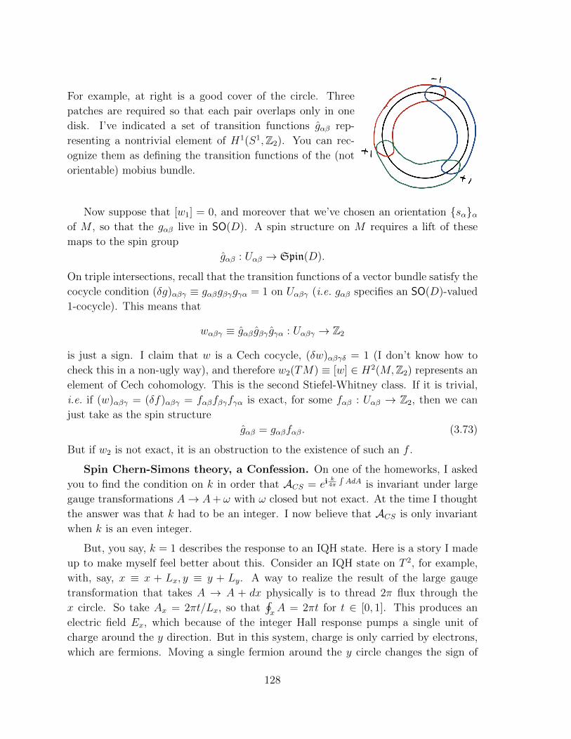
For example, at right is a good cover of the circle. Three
patches are required so that each pair overlaps only in one
disk. I’ve indicated a set of transition functions gαβ rep-
resenting a nontrivial element of H1(S1,Z2). You can rec-
ognize them as defining the transition functions of the (not
orientable) mobius bundle.
Now suppose that [w1] = 0, and moreover that we’ve chosen an orientation sααof M , so that the gαβ live in SO(D). A spin structure on M requires a lift of these
maps to the spin group
gαβ : Uαβ → Spin(D).
On triple intersections, recall that the transition functions of a vector bundle satisfy the
cocycle condition (δg)αβγ ≡ gαβgβγgγα = 1 on Uαβγ (i.e. gαβ specifies an SO(D)-valued
1-cocycle). This means that
wαβγ ≡ gαβ gβγ gγα : Uαβγ → Z2
is just a sign. I claim that w is a Cech cocycle, (δw)αβγδ = 1 (I don’t know how to
check this in a non-ugly way), and therefore w2(TM) ≡ [w] ∈ H2(M,Z2) represents an
element of Cech cohomology. This is the second Stiefel-Whitney class. If it is trivial,
i.e. if (w)αβγ = (δf)αβγ = fαβfβγfγα is exact, for some fαβ : Uαβ → Z2, then we can
just take as the spin structure
gαβ = gαβfαβ. (3.73)
But if w2 is not exact, it is an obstruction to the existence of such an f .
Spin Chern-Simons theory, a Confession. On one of the homeworks, I asked
you to find the condition on k in order that ACS = eik4π
∫AdA is invariant under large
gauge transformations A→ A+ ω with ω closed but not exact. At the time I thought
the answer was that k had to be an integer. I now believe that ACS is only invariant
when k is an even integer.
But, you say, k = 1 describes the response to an IQH state. Here is a story I made
up to make myself feel better about this. Consider an IQH state on T 2, for example,
with, say, x ≡ x + Lx, y ≡ y + Ly. A way to realize the result of the large gauge
transformation that takes A → A + dx physically is to thread 2π flux through the
x circle. So take Ax = 2πt/Lx, so that∮xA = 2πt for t ∈ [0, 1]. This produces an
electric field Ex, which because of the integer Hall response pumps a single unit of
charge around the y direction. But in this system, charge is only carried by electrons,
which are fermions. Moving a single fermion around the y circle changes the sign of
128

the wavefunction, or not, depending on the choice of spin structure. The default spin
structure, the easier one to describe, is the one with antiperiodic boundary conditions
on the fermions. So we can attribute the sign acquired by the amplitude during the
large gauge transformation to this sign from the choice of spin structure.
3.6 Characteristic classes and classifying spaces
Stiefel-Whitney classes of TM are examples of a more general notion of characteristic
classes of a bundle. There are many ways to think about characteristic classes. Here is
one: The topology of a G-bundle on M can be specified by a map γ : M → BG. This
is the point in life of the classifying space BG. Such a space exists for each G. But
then each cohomology class of BG produces a cohomology class on M via the pullback:
γ? : Hn(BG,A)→ Hn(M,A) (3.74)
(for any abelian group A). The images of this map are characteristic classes.
Classifying space and universal bundle. One way to think about this is that
there is a universal G-bundle with total space EG
G EG
BG
ξ
(3.75)
with the property that any bundle on X is the pullback of ξ via the map γ : X → BG.
(The fiber over the point x ∈ X is ξ−1(γ(x)).) BG is determined (up to homotopy) by
demanding that EG is contractible and admits a free G action. Essentially, it’s always
some kind of infinite-dimensional sphere. For example, for G = U(1), it’s the limit of
the Hopf fibration as the dimension goes to ∞.
U(1) S2∞+1
CP∞ = BU(1)
Z2 S∞
RP∞ = BZ2
SU(2) S4∞+1
HP∞ = BSU(2)
Note that for bundles on X of dimension < k we actually only really care that πq<k(EG)
vanishes, and so in practice we can just think about high-dimensional spheres and
they’ll do just as well.
By the way, here’s a nice use of the classifying space to define the Dijgraaf-Witten
path integral for a discrete G gauge theory with a cocycle ν ∈ HD(G,U(1)). The group
129

cohomology we defined above is in fact related to the ordinary cohomology of BG 54.
For discrete G the relation is just
HD(BG,U(1)) = HD(G,U(1)) (3.76)
(these very similar-looking objects have very different definitions!). So if spacetime M
is divided up into a simplicial complex (with a branching structure), we specify a gauge
field configuration by a map γ : T → BG for each simplex T , and the cocycle ν ∈HD(BG,U(1)) associates a phase ν(γ(T )). The amplitude (summand of the partition
function of the DW theory is then just
W [γ] =∏T
νs(T )(γ(T )) (3.77)
where s(T ) is the same sign choice as above55. Note that W [γ] is (a discrete representa-
tive of) the characteristic class defined by the pullback of the class ν ∈ HD(BG,U(1))
via the map γ. In fact, the relation between (3.77) and the group cohomology SPT
construction above is the best way to understand the equation (3.76).
A second perspective, more obviously related to what we said in the discussion of
spin structures, is from obstruction theory: try to construct a nowhere-zero section of
the bundle V in question. Approximate M by a cell complex. First find a solution on
the 0-cells. Then try to extend this solution from the p-cells to the p+ 1-cells: suppose
given a vector field on Sp = ∂Bp+1, that is, a map Sp → Rm (where m is the rank of the
bundle, and I’m supposing that it’s a bundle over R for example), can it be extended
to the interior of the ball? The bundle itself can trivially be extended to Bp=1, since
π•(B) = 0. But demanding that the vector field is nowhere zero means that this map
is homotopic to a map Sp → Sm−1. For p + 1 < m, this is fine, but for p + 1 = m,
there is a winding number, the degree of the map, which if it’s nontrivial obstructs
the extension to the interior. So we have an integer for each m-cell, an element of
Hm(M,Z). This thing mod two is wm(V ), the Euler class of the bundle V . Or: This
54In general, the relation is HD(G,U(1)) = HD+1(BG,Z); for discrete G, this is the same as
HD(BG,U(1)) by the long exact sequence associated to Z → R → U(1), using the fact that for
discrete G, H•(BG,R) = 0.55Actually there is one more step: we must show that the partition function actually only depends on
a configuration of link variables gσ specifying a flat connection. The key idea is that a configuration
of the link variables specifies a map γ : M → BG because of the homotopy equivalence of ΩBG
and G. (This is consistent with π1(BG) = π1(EG/G) = G = π0(G) and with BG = K(G, 1) and
G = K(G, 0).) Define γ to take all 0-cells to the base point of BG. A link-variable configuration
gσσ∈M1associates an element of G to each edge, and hence a homotopy class of closed paths in BG
(starting and ending at the base point). Then the flatness of the connection allows us to extend this
map to all the higher-dimensional cells.
130

failure to construct a nowhere-zero section means that any actual section has zeros.
This locus of zeros gives the Poincare dual of wm(V ).
If we instead try to construct q linearly-independent nowhere-zero sections, we can
orthogonolize the sections and produce a map Sp → Sm−q, which gives an element of
Hm−q(M,Z2), which is the wm−q(V ). The Poincare dual to this is the locus of points
where the sections fail to be linearly independent.
I haven’t shown that this definition is the same as the definition in terms of Cech
cohomology above.
Actually there are some very simple examples of characteristic classes. Let’s think
about the case of a complex vector bundle V over X. Then choose a connection A on
V . Let’s call G ⊂ U(N) the structure group of V . Now make a G-invariant polynomial
in F = dA+ A ∧ A, where G acts by F → g−1Fg. For example,
c(G) ≡ det
(1 +
iF
2π
)= 1 + c1(F ) + c2(F ) + · · ·
is the sum of symmetric polynomials in the eigenvalues of F called the total Chern
class of F . cj(F ) is the degree-j part of c(F ) and is a 2j-form. Some properties of
these objects that I will not prove:
1. dc(F ) = 0, so these forms all cohomology classes on the base manifold X.
2. Their integrals∮Sc(F ) over closed cycles S ⊂ X depend only on the transition
functions of the bundle V and not on the choice of connection. This is because
given two connections A0,1 one can take a convex combination of them (At =
A0 + t(A0 − A1), Ft = dAt + A2t ) and show that the difference of their Chern
classes is exact:
cm(F1) = cm(F0) = md
∫ 1
0
dttr(A0 − A1) ∧ Fm−1t .
For an elementary proof of this statement, see Harvey’s anomaly lectures.
3. The total Chern class behaves nicely under the direct sum operation on bundles:
c(V ⊕ V ′) = c(V ) ∧ c(V ′). (3.78)
So for example, c2(V ⊕ V ′) = c2(V ) + c2(V ′) + c1(V ) ∧ c1(V ′). Notice that this
relation (3.78) implies that the Chern classes are stable under the addition of
trivial bundles c (V ⊕ trivial ) = c(V ).
131

For real bundles, F is a real antisymmetric matrix, and it is better to define instead
p(F ) = det
(1− F
2π
)= 1 + p1 + p2 + · · ·
where the degree-2j bit pj is a 4j form. p is for Pontryagin.
132

3.7 Classification of SPTs, part one
[I found this document very helpful.] Stacking is something we can do with anything.
Given two physical systems A and B, we can make A+B just by putting A and B on
top of each other. If A and B are specified by G-preserving, gapped groundstates of
G-symmetric Hamiltonians with an energy gap, then A+B is, too.
To be a little more precise, let’s sayMdG is the space of deformation classes of triples
(H, ρ,H), where H is a Hilbert space made as a tensor product (or, for fermions, a
graded tensor product) on a d-dimensional lattice, ρ is a representation of G on the
Hilbert space H, and H is a local hamiltonian on H. By deformation classes, we can
mean adding ancillas and adiabatic variation without closing the gap.
So stacking means HA+B = HA ⊕ HB, ρA+B = ρA ⊕ ρB, and HA+B = HA + HB,
and then we are allowed to deform while preserving the gap. Stacking with the trivial
phase does nothing. So stacking givesMdG the structure of a ‘monoid’ – a group except
for inverses.
A better definition of SPTs with G symmetry in d dimensions is
SPTdG ≡ invertible elements of Md
G . (3.79)
Thus SPTdG is a group, essentially by definition. Moreover, it is not too hard to see that
MdG is associative and commutative. Basically it’s just because H1 ⊕H2 = H2 ⊕H1.
Therefore SPTdG is an abelian group. Discrete abelian groups are pretty simple. How
can we resist asking: for a given G, d (and specification of the microscopic constituents,
i.e. is it made of bosons or fermions) which one is it?
But first, some important comments about this definition. This definition is differ-
ent from (a definition of SPTs that was made in the earlier literature)
SREdG ≡G-symmetric non-SSB systems
that can be deformed to the trivial state while preserving the gap,
but not through G-symmetric Hamiltonians.
SRE stands for ‘short-range-entangled’, and my notation here is not standard. SREdG
is a subgroup of SPTdG (and in fact a direct summand).
Why is definition (3.79) is better? The condition of invertibility is weaker than
deformability to the trivial phase in the absence of symmetry, but it still implies the
absence of anyons (since obviously you can’t get rid of anyons by adding more anyons).
It should therefore also imply a unique groundstate on any closed manifold. These
properties are easier to check than deformability to the trivial phase.
133

Nontrivial invertible states with no symmetry. Unlike SREdG, our definition
of SPTdG is nontrivial even when G = e is the group with one element. Such systems
are protected instead by a gravitational anomaly. For fermions, examples of such states
are the following:
• In D = 2 + 1, a p + ip superconductor, two copies of which are an IQH system
after the U(1) symmetry is broken. In this case, the central charge of the edge
modes indicates the gravitational anomaly.
• In D = 1 + 1, the Kitaev chain. Oh there is a lot to say about this.
• In D = 0 + 1, an odd number of majorana modes. You can see that there is a Z2
classification of such states, since, given two majorana modes, the perturbation
H = iγ1γ2 lifts both of them.
For bosons, the first example is the E8 state in D = 2 + 1. Our description of this
state is abelian CS theory with K-matrix equal to the Cartan matrix of the Lie algebra
E8. What’s special about E8? The E8 lattice has the remarkable property that it is
even and self-dual. Lattices with both of these properties only occur in dimensions
that are multiples of 8. (These are the same reasons that E8 plays an important role
in string theory.) These properties imply in particular that | detK| = 1, so there is a
unique groundstate on any Riemann surface, and that all the quasiparticles are bosons.
So there is no topological order.
Functorial properties. Think of SPTdG as a machine that eats a group G and
spits out a discrete abelian group. In trying to figure out what this machine does,
the following observation is valuable: In fact SPTd• is a (contravariant) functor, from
groups to groups. That means that it maps the structure of the victim to the structure
of the output: given a group homomorphism ϕ : H → G, there is automatically a
group homomorphism ϕ? : SPTdG → SPTd
H . (The fact that the arrows get reversed is
the reason for the adjective ‘contravariant’.)
Despite the intimidating words, this is simple. First consider the case where the
homomorphism is just inclusion of a subgroup: Hi−→ G. Then [A] ∈ SPTd
G is also
[A] ∈ SPTdH , since anything G-symmetric is also H ⊂ G-symmetric. (Note that
a nontrivial G-SPT could be trivial as an H-SPT.) More generally, given a group
homomorphism ϕ : H → G and a G-SPT, (H, ρ,H), we can make an H-SPT by
ϕ?(H, ρ,H) = [(H, ρ ϕ,H)]. (3.80)
Notice that
ρ ϕ : Hϕ−→ G
ρ−→ U(H) (3.81)
(where U(H) means unitaries on H) is a rep of H.
134

3.8 Global anomaly inflow
[We’ll follow Witten for a bit. I found this paper by Garcıa Extebarria and Montero
very useful.]
How to discover that anomalies are encoded in an extra-dimensional
theory. Let me return once more to the gapless edge theory of a (3 + 1)D TI with
G = U(1) n ZT2 . A mass term for the Dirac fermion breaks time-reversal symmetry.
With two such modes,∫
iη1η2 would be T -invariant, so there is a Z2 classification of
anomalous theories. One way to think about this is that if we can add a symmetric
mass term, we can use Pauli-Villars regularization to define the path integral in a
manifestly symmetric way so there can be no anomaly.
Let’s think about trying to define the path integral for η on some oriented spacetime
X:
ZX = det (D) , D ≡ iγµDµ.
This dirac operator D = D† is hermitian and so has real eigenvalues, so ZX =∏
i λi ∈R. This is a consequence of T -invariance: in general, for an oriented manifold X,
Z?(X) = Z(X), where X has the reversed orientation. With two Dirac fermions, the
partition function would be Z2X =
∏i λ
2i > 0 would be positive, but with one copy the
sign of ZX is not fixed:
signZX = (−1)#of negative eigenvalues of D mod two.
In the continuum, the object in the exponent is infinity. Note that if we are willing to
break T and add a mass, then there is no problem defining the sign of ZX .
You might not think to care about the sign of ZX , and think that we can just
declare it to be positive. But here’s why it’s non-trivial: just declaring it to be positive
is not a gauge-invariant choice. ZX here is really a functional of the background fields
(g, A), where A is the background U(1) gauge field and g is the metric on X. Suppose
we declare Z(g0, A0) > 0 for some reference background. Then we define the sign
of Z(g, A) for general (g, A) by finding a path from (g0, A0) to (g, A) in the space of
background fields. Z changes sign whenever an eigenvalue λ crosses 0 along this path.
But: let φ be some gauge transformation (or coordinate change, i.e. diffeomor-
phism), under which (g0, A0)→ (gφ0 , Aφ0). Then
As = (1− s)A0 + sAφ0 , gs = (1− s)g0 + sgφ0
is an allowed background for s ∈ [0, 1] (note that gs > 0 if g0,1 > 0). Now we can ask:
as we vary s, how many eigenvalues cross 0?
135

Gauge invariance of our definition requires an even number.
The fact that φ is a gauge transformation means that the
spectrum of D is the same at s = 0, 1. But the fact that the
spectrum goes off to infinity means that a given eigenvalue
need not return to itself – there can be spectral flow.
There is an index formula for the net number ∆ of eigenvalues crossing λ = 0, so
Z(g0, A0) = (−1)∆Z(gφ0 , Aφ0).
The formula is ∆ = I where I is the index of a (3 + 1)D Dirac operator D on the
following 4-manifold, Yφ. Yφ is called the mapping torus:
Y = I ×X/(0, x) ∼ φ(0, x)
where φ here is the action of φ on the metric. The same identification on As determines
a U(1) connection (and bundle) on Yφ. (If φ acts only as a gauge transformation and
not a diffeomorphism, then the space Yφ is just S1 ×X.)
The conclusion here is that ZX(g, A) is not a function on the space of background
fields, but rather a section of some bundle with structure group Z2. The nontriviality
of this bundle is what makes the theory anomalous. (In this example, it says either we
have to give up T or we have to give up gauge invariance.)
So we have an association between our anomaly (manifesting itself as a difficulty
in defining the sign of the path integral on X) in D− 1 dimensions, and a field theory
in D dimensions. One way to think about the association is that if we coupled the
two of them together, there would be no anomaly – this is anomaly inflow. So to
understand ZX , we can find a manifold Y with ∂Y = X and extend the gauge bundle
on X to Y and put the ‘anomaly theory’ on Y . In this case the ‘anomaly theory’ is a
(3 + 1)D massive Dirac fermion with M < 0. Think about the bulk path integral on a
background configuration with Dirac index I: this means, generically that there are I
left-handed zeromodes ψi+ (and their conjugates ψi−. The path integral is then of the
form
Zbulk =
∫[DΨ]e
∫Ψ(iD−M)Ψ+··· ∝
∫dψ1
+ · · · dψI+dψ
1− · · · dψI
−eMψ−ψ+ = MI.
In the TI phase, M < 0, so the sign of this path integral is indeed (−1)I.
Now let’s generalize. We want to identify possible anomalies of a system in D −1 spacetime dimensions: failures of the effective action (as a functional of general
background fields, on general manifolds) to be gauge invariant. Such a system is
136

then a candidate for a characteristic surface state of an SPT in D dimensions. The
construction here will incorporate the D dimensional theory quite organically.
To begin, suppose we wish to understand the partition function ZX of our putative
anomalous theory on X, a D−1 manifold. ZX is a section of a nontrivial bundle on the
space of background fields. The first step is to find a D-manifold Y with ∂Y = X56.
Any structure that we care about, such as a background
gauge field or a spin structure on X we must also extend
to Y . The key idea is that there is a quantity associated
with Y that’s a section of the same bundle – it’s the par-
tition function of the associated ‘anomaly theory’, i.e. the
bulk SPT.
In the case where the anomalous edge theory in question is just free fermions, the
‘anomaly theory’ is a massive fermion in one extra dimension. The dynamics of the
massive fermion are not important at all here, and sometimes the ‘theory’ is described
as just an association of a phase to each D-manifold, called the η-invariant:
e2πiηY ≡ partition function of SPT on Y
(with boundary conditions compatible with X).
To get started at appreciating this idea, note that it incorporates all the perturbative
(or ‘local’) anomalies of fermions by taking Y = ∂Z, Z = X ×D (D is a disk). Then
the APS index theorem for manifolds with boundary says that the index of the Dirac
operator on Z is
Z 3 Ind (iDZ) = ηY +
∫Z
A(R) ∧ treF2π
which says
e2πiηY = exp
(2πi
∫Z
(A(R) ∧ tre
F2π
)D+2
)= e2πi
∫Z ID+1 (3.82)
whose variation, by the WZ descent procedure, reproduces the chiral anomaly in D−1
dimensions.
Any anomaly in a gauge transformation not continuously connected to the identity
is called a global anomaly. Such a gauge transformation is a map from spacetime X
to G. Homotopy classes of such maps are denoted [X,G]. For example, the one-point
compactification of Rd is X = Sd, and [Sd, G] ∼ πd(G) (under some assumptions about
G). For example, in a system in d = 3 + 1, with G = SU(2), we have π4(SU(2)) = Z2
and there is an interesting possibility of an SU(2) anomaly.
56In fact, not all X admit such a Y . What to do in that case I hope to explain below. If I fail, see
section 6 of the Garcıa-Etxebarria and Montero paper.
137

The η invariant has some nice properties that we want for any SPT: If we can
decompose M = Y1 ∪ Y2 as the result of gluing two open manifolds along cancelling
boundaries (∂Y1 = −∂Y2), then
e2πiηY1∪Y2 = e2πiηY1e2πiηY2 . (3.83)
So for example the change of phase from Z[A0] to Z[Aφ0 ] is
Z[Aφ0 ] = e2πiηX×IZ[A0].
This means that this idea incorporates the mapping-torus global anomaly we discussed
above.
More general anomalies. Now if the partition function of the anomaly theory on
a mapping torus is not equal to one, it clearly represents a failure of gauge invariance
of the theory on X. But what about the partition function of the anomaly theory on
other manifolds?Take any closed D-manifold Y and chop it into two parts:
Y = Y1 ∪ Y2 with ∂Y1 = X = −∂Y2. Then Y1 and Y2 each
represent a possible extension of X that could be use to de-
fine the partition function of the edge theory on X. But if
ei2πη(Y1∪Y2) 6= 1, it means that the answer for the partition
function on X depends on the extension to Y ! So this is
also an anomaly. (Sometimes this case is called a Dai-Freed
anomaly.)
For the case of free fermions, if the local anomalies vanish (this means the anomaly
polynomial I = 0), then ηY is topological, and moreover is a bordism invariant. To see
this, suppose Y1 is bordant to Y2. This means that there exists Z with ∂Z = Y1 q Y2
(that symbol q means disjoint union). Now use (3.83) to write
e2πiηY1qY2 =e2πiηY
e2πiηY2
(3.82)= e2πi
∫Z ID+2 = 1 (3.84)
by the assumption of no local anomalies. In the first step of (3.84) we used the fact
that e2πiηY = e−2πiηY .
138
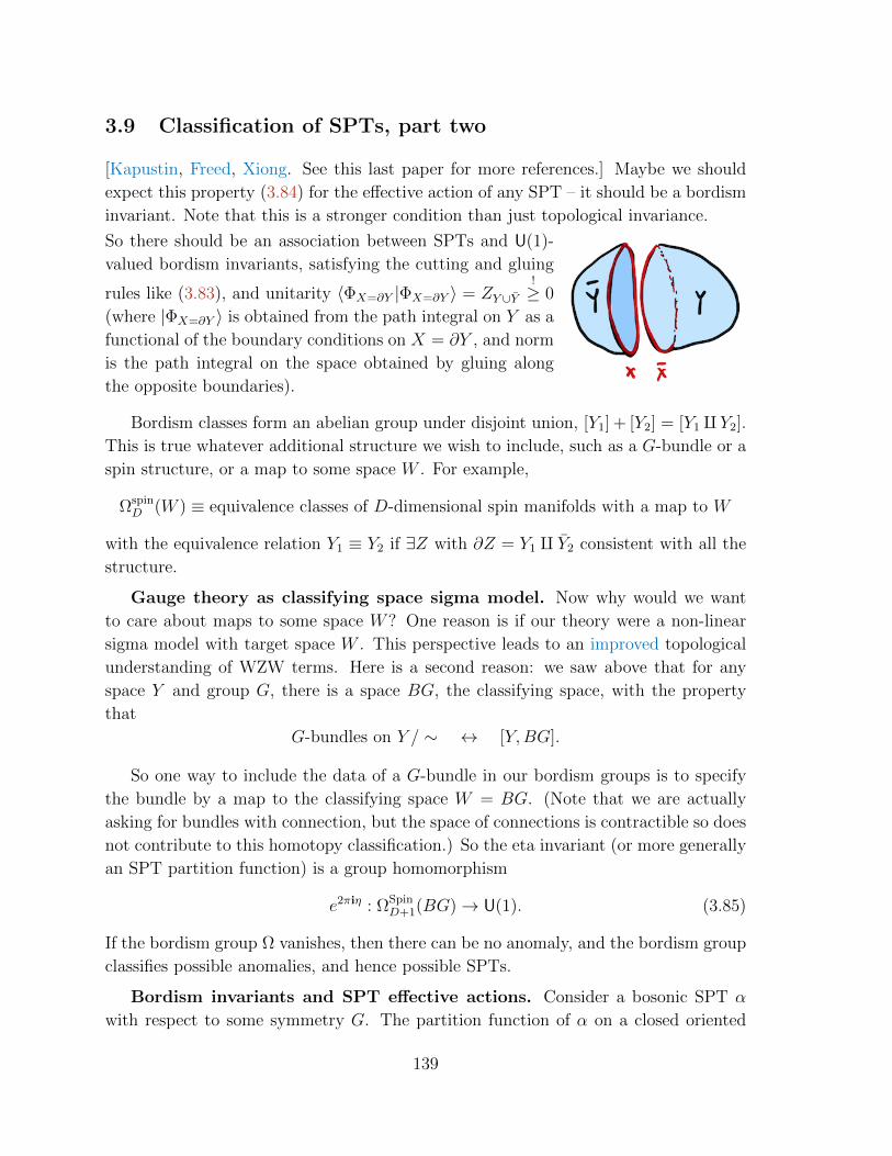
3.9 Classification of SPTs, part two
[Kapustin, Freed, Xiong. See this last paper for more references.] Maybe we should
expect this property (3.84) for the effective action of any SPT – it should be a bordism
invariant. Note that this is a stronger condition than just topological invariance.
So there should be an association between SPTs and U(1)-
valued bordism invariants, satisfying the cutting and gluing
rules like (3.83), and unitarity 〈ΦX=∂Y |ΦX=∂Y 〉 = ZY ∪Y!
≥ 0
(where |ΦX=∂Y 〉 is obtained from the path integral on Y as a
functional of the boundary conditions on X = ∂Y , and norm
is the path integral on the space obtained by gluing along
the opposite boundaries).
Bordism classes form an abelian group under disjoint union, [Y1] + [Y2] = [Y1 q Y2].
This is true whatever additional structure we wish to include, such as a G-bundle or a
spin structure, or a map to some space W . For example,
ΩspinD (W ) ≡ equivalence classes of D-dimensional spin manifolds with a map to W
with the equivalence relation Y1 ≡ Y2 if ∃Z with ∂Z = Y1 q Y2 consistent with all the
structure.
Gauge theory as classifying space sigma model. Now why would we want
to care about maps to some space W? One reason is if our theory were a non-linear
sigma model with target space W . This perspective leads to an improved topological
understanding of WZW terms. Here is a second reason: we saw above that for any
space Y and group G, there is a space BG, the classifying space, with the property
that
G-bundles on Y / ∼ ↔ [Y,BG].
So one way to include the data of a G-bundle in our bordism groups is to specify
the bundle by a map to the classifying space W = BG. (Note that we are actually
asking for bundles with connection, but the space of connections is contractible so does
not contribute to this homotopy classification.) So the eta invariant (or more generally
an SPT partition function) is a group homomorphism
e2πiη : ΩSpinD+1(BG)→ U(1). (3.85)
If the bordism group Ω vanishes, then there can be no anomaly, and the bordism group
classifies possible anomalies, and hence possible SPTs.
Bordism invariants and SPT effective actions. Consider a bosonic SPT α
with respect to some symmetry G. The partition function of α on a closed oriented
139

manifold Y with background fields for G is e2πiSαY [A]. Some properties of this functional
follow from our assumptions:
• Since the phase α is gapped, SαY is a local functional of the background gauge
field A and the metric, and it’s gauge invariant. Terms whose coefficient we can
vary continuously while preserving these properties (like a Maxwell term) don’t
label the phase.
• Since α has a unique groundstate on any closed spatial slice, the amplitude
e2πiSαY [A] must be a phase57.
• SαY
[A] = −SαY [A] by the CPT theorem.
• SY1qY2 = SαY1+ SαY2
.
• SαY [A] = SαY
[A] where α is the inverse SPT phase.
What terms can appear in SαY [A] =∫Y
∑i Lαi ? If the variation of a term in S with
respect to gµν vanishes, then that term is said to be topological. There can certainly be
non-topological terms, like a Maxwell term. A less innocuous non-topological term is
a gravitational Chern-Simons term. Such terms occur in D = 4n− 1; in D = 3, such a
term produces a thermal Hall response κxy. In the SPT group law, any two SPTs with
the same κxy differ by an SPT with κxy = 0. So let’s first classify SPTs with κxy = 0.
So let’s focus on the topological terms in SαY [A]. How can the effective action depend
on the topology of Y and the G-bundle on it?
• No symmetry. First, suppose the protecting symmetry is nothing, G = e.The fact that there is no time-reversal symmetry means that Y must be oriented.
Sα then depends on the topology of Y through local integrals. This must be a
sum of integrals of products of characteristic classes of TY . These are Pontryagin
classes (in degrees that are multiples of 4) and Stiefel-Whitney classes (in all
degrees, but just mod two). Such sums of integrals of their products are called
Pontryagin and Stiefel-Whitney numbers of Y . These numbers depend only on
the bordism class of Y . In fact, Thom proved that they also determine the
bordism class of Y .
57To see this, slice an arbitrary D-dimensional Y along some closed D − 1 manifold Σ into Y =
Y1 ∪Σ Y2, so we can write ZY = 〈Y1|Y2〉, in terms of some normalized states |Y1,2〉. Since dimHΣ = 1,
we have, using the magic of 1d linear algebra,
|ZY |2 = 〈Y1|Y2〉 〈Y2|Y1〉 = 〈Y1|Y1〉 〈Y2|Y2〉 = 1.
140

So in this case the effective action is a group homomorphism
e2πiSαY : ΩD,SO(pt)→ U(1).
The SO subscript indicates that the structure group of Y is SO(D). The fact that
SY is additive under disjoint union implies that it is a group homomorphism. The
group of homomorphisms from ΩD to U(1) can be called the cobordism group
ΩDSO(pt,U(1)) ≡ Hom(ΩD,SO(pt)→ U(1)). (3.86)
But the abelian group ΩD,SO(pt) can include a free part. The associated terms
are like theta terms with continuously-variable coefficient that don’t label the
phase. So we expect bosonic SPT phases with no symmetry to correspond to
bSPTDG=e = ΩD
SO(pt,U(1))/ΩDSO(pt,R).
These are the SPTs missing from the SRE subgroup.
• Time-reversal symmetric phases. If G = ZT2 , then Y can be unoriented.
This also means that α = α, and 2SαY [A] = 0 mod 1, that is, SαY [A] = 0, 12
mod 1,
so all phases are order two. The bordism invariants are just the Stiefel-Whitney
classes, also all mod two, so there is no free part. So we expect
bSPTDG=ZT2
= ΩDO (pt,U(1)).
• General unitary G. The background gauge field specifies a map γ : Y → BG,
and so we can demand that our cobordisms include an extension of this map:
bSPTDG = ΩD
SO(BG,U(1))/ΩDSO(BG,R).
• General symmetry. If the symmetry includes time-reversing elements, we can
specify them by a homomorphism ρ : G → Z2, with ker ρ is the unitary part of
the group. ρ induces a map BG→ BZ2, and hence a pullback Z of the universal
Z2-bundle to BG. A background gauge field configuration γ for G must have the
property that the pullback γ?(Z) is the orientation bundle of Y .
Let’s think about the case G = ZT2 in more detail. The formal sum of unoriented
bordism groups over dimension is a nice graded algebra of polynomials Ω•O(pt) =
Z2[xj] with generators xj of degree j = 2, 4, 5, 6, 8... (that is, not 2i − 1). This is a
result of Thom that I will not prove. This means that the groups are:
D 1 2 3 4 5
ΩD,O(pt) 0 Z2 0 Z2 × Z2 Z2
We can associate them with particular combinations of Stiefel-Whitney classes. We’ve
seen the associated phases already in this class.
141

• The result in D = 1 + 1 comes from the invariant∫Yw2
1 =∫Yw2 = the euler
character of Y mod two. This means that ZY = e2πi( 12
∫Y w2(Y )) = eiπχ(Y ) = ±1
according to whether or not Y is orientable. This is the Haldane chain.
• In D = 2 + 1 the SW classes satisfy the relations w1w2 = w3 = w31 = 0 for
all closed 3-manifolds. This is consistent with the statement that every such
3-manifold is null-bordant – the boundary of some 4-manifold.
• In D = 3 + 1, the relations w3w1 = w2w21 = 0 and w4 + w2
2 + w41 = 0 leave two
independent invariants that we can take to be 12w4
1 and w22. This means three
nontrivial bosonic SPTs for time-reversal symmetry (two nontrivial generating
phases and their stacking). These are just the phases we saw from the coupled-
layer construction. The one corresponding to w22 is the one we discussed more
explicitly, whose surface is the all-fermion toric code (this phase is called efmf
by Wang and Senthil). This makes sense because if there are neutral fermions, we
can only put the system on a spin manifold, which has w2 = 0: hence the anomaly
disappears in the presence of neutral fermions. The other one, corresponding to12w4
1, is the one visible in group cohomology, and has a surface which is the toric
code where e and m are both Kramers’ doublets (called eTmT by Wang and
Senthil).
• Finally inD = 4+1, the nontrivial invariant is 12
∫w2w3, whereasH4(BZ2,U(1)) =
0. This phase survives the breaking of time-reversal symmetry. It has a surface
given by all-fermion electrodynamics, and an effective description in terms of
2-form CS gauge theory with action S[B,C] =∫YB∧dC
2π.
Generalized cohomology and loop spectrum. These bordism groups are an
example of a generalized cohomology theory. There is a set of seven axioms due to
Eilenberg and Steenrod defining what is a cohomology theory. It is a contravariant
functor from topological spaces to abelian groups, just like SPTGD. The usual de Rham
and Cech theories satisfy all of these axioms. A generalized cohomology theory fails
to satisfy the last axiom, which demands that H•(point) is trivial. This is where the
non-SRE states come in.
[End of Lecture 20]
A spectrum (or loop spectrum or Ω-spectrum) is a machine for producing a general-
ized cohomology theory. It is a family of topological spaces Kd, labelled by d ∈ Z with
property that Kd ' ΩKd+1, where ΩX means the loop space of X, and the relation is
homotopy equivalence. Given such a spectrum K•, the generalized cohomology groups
associated with K• are defined to be
Hd(X,K) ≡ [X,Kd]
142
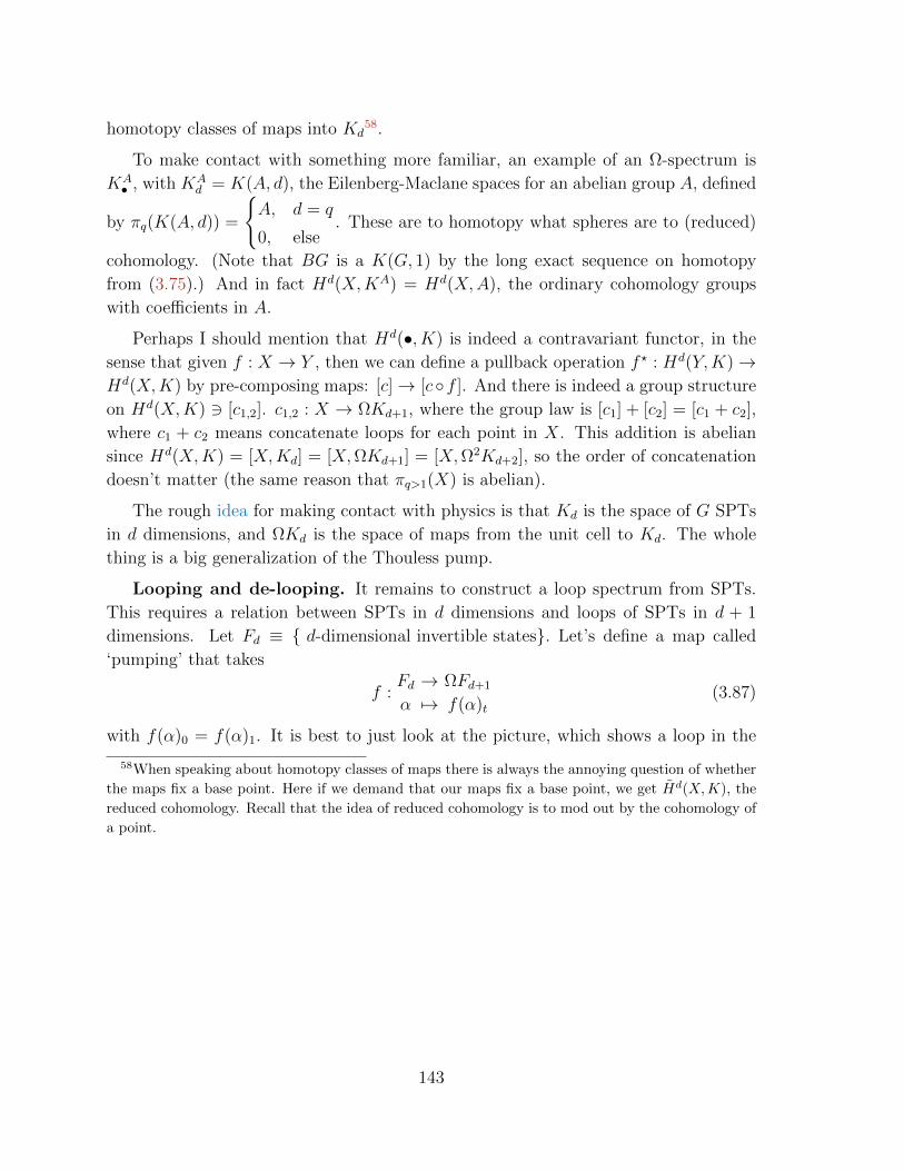
homotopy classes of maps into Kd58.
To make contact with something more familiar, an example of an Ω-spectrum is
KA• , with KA
d = K(A, d), the Eilenberg-Maclane spaces for an abelian group A, defined
by πq(K(A, d)) =
A, d = q
0, else. These are to homotopy what spheres are to (reduced)
cohomology. (Note that BG is a K(G, 1) by the long exact sequence on homotopy
from (3.75).) And in fact Hd(X,KA) = Hd(X,A), the ordinary cohomology groups
with coefficients in A.
Perhaps I should mention that Hd(•, K) is indeed a contravariant functor, in the
sense that given f : X → Y , then we can define a pullback operation f ? : Hd(Y,K)→Hd(X,K) by pre-composing maps: [c]→ [cf ]. And there is indeed a group structure
on Hd(X,K) 3 [c1,2]. c1,2 : X → ΩKd+1, where the group law is [c1] + [c2] = [c1 + c2],
where c1 + c2 means concatenate loops for each point in X. This addition is abelian
since Hd(X,K) = [X,Kd] = [X,ΩKd+1] = [X,Ω2Kd+2], so the order of concatenation
doesn’t matter (the same reason that πq>1(X) is abelian).
The rough idea for making contact with physics is that Kd is the space of G SPTs
in d dimensions, and ΩKd is the space of maps from the unit cell to Kd. The whole
thing is a big generalization of the Thouless pump.
Looping and de-looping. It remains to construct a loop spectrum from SPTs.
This requires a relation between SPTs in d dimensions and loops of SPTs in d + 1
dimensions. Let Fd ≡ d-dimensional invertible states. Let’s define a map called
‘pumping’ that takes
f :Fd → ΩFd+1
α 7→ f(α)t(3.87)
with f(α)0 = f(α)1. It is best to just look at the picture, which shows a loop in the
58When speaking about homotopy classes of maps there is always the annoying question of whether
the maps fix a base point. Here if we demand that our maps fix a base point, we get Hd(X,K), the
reduced cohomology. Recall that the idea of reduced cohomology is to mod out by the cohomology of
a point.
143

space of invertible states in d+ 1 dimensions:
Here y is the extra dimension.
And we can define a map going the other way
g :ΩFd+1 → Fdβ(t) 7→ g(β)
(3.88)
by cutting the system open at some particular point in x. g(b) is the d-dimensional
SPT that is pumped past the cut to the right.
Claims: f and g are homotopy inverses. g f = 1 by construction, and f g ' 1.
Concatenation of loops β1(t), β2(t) in ΩFd+1 maps to stacking of d-dimensional
SPTs, g(β1,2).
So the current understanding is that
SPTdG = Hd(BG,K) (3.89)
for some Ω-spectrum K. As we discussed above, the group cohomology H•(G,U(1)) is
related to the ordinary cohomology of BG. So just as the homotopy groups are different
from the cohomology groups of a space, this improved classification will both add and
remove SPTs relative to the states that were explicitly constructed in 3.4.
If we take K to be the Thom spectrum (which I’m not going to say what it is), we
get the cobordism classification motivated above. A nice thing about this perspective
is that as our understanding of the space of invertible states Fd grows, we can improve
our classification.
144