physics 1210 lab manual 1210 laboratory manual ... the water’s speed at 25.0 m/s. at point b, ......

PHYSICS 1210

LAB MANUAL

ACKNOWLEDGMENTS

Most of the experiments in the Physics 1210 Lab Manual were adapted from the Physics 111 Lab Manual, which was the work of Dr. Michael Ziegler, Prof. Klaus Honscheid, Prof. R. Sooryakumar, Dr. Kathy Harper, and Michael Smyser. Experiment 2 originally was adapted for Physics 111 from an experiment designed by Prof. Douglas Schumacher for Physics 131. Prof. Thomas Humanic submitted recommendations for upgrading the Physics 111 labs for Physics 1200 in June 2011. Experiments 9, 10, and 11 were adapted from the Physics 113 Lab Manual, which was the work of Prof. Greg Lafyatis, Prof. Jay Gupta, Dr. Michael Ziegler, and Ai Binh Ho. Experiment 5 was developed by Prof. Tom Humanic during the winter and spring of 2012. The laboratory equipment setups for all labs in this manual were reviewed during spring and summer 2012 by Harold Whitt and staff, and by Daniel Erickson. Revised in spring-summer 2013 by Dr. Michael Ziegler based on input from Dr. Raju Nandyala, Harold Whitt, and Dr. Jesse Martin. Revised in spring-summer 2014 by Dr. Michael Ziegler based on lab instructor input.

Copyright© by the Department of Physics, The Ohio State University, 2014.

Physics 1210 Laboratory Manual

Table of Contents Experiment 9: Fluids Lab Challenge: Determination of Mass Density Experiment 10: Simple Harmonic Motion Lab Challenge: Find the unknown mass. Experiment 11: Introduction to Waves and Addition of Waves Lab Challenge: none Appendix B: Introduction to LoggerPro Appendix C: Equipment for Laboratory Experiments

Physics 1200 IX-1

Name ________________________________

Partner(s): ________________________________

Experiment 9: Fluids Objectives Study Pressure, Buoyancy force, Fluids in motion Equipment Computer with LoggerPro, Force Probe, and Venturi Tube Preparation You will be pressed for time during the lab. Since successful completion of all lab

activities counts towards your final lab grade it will be important to be well prepared by doing Pre-Lab assignments and reading the entire lab before attending the lab.

Pre-Lab Read the Pre-Lab introduction and answer the accompanying questions and

problems before this Lab.

Points earned today Pre-Lab ____ Lab ____ Challenge ____ Total ____ Instructor Initials ____ Date ____

IX - 2 Physics 1200

Pre-Lab for LAB#9

Intro A fluid may be a liquid or a gas. In this lab we look at the behavior of static (non-moving) fluids and dynamic (moving) fluids.

Static Behavior of Fluids According to Pascal’s principle, if an external pressure Po, such as air pressure, acts

on a fluid, that pressure is transmitted throughout the fluid without change. In addition, for a fluid in a gravity field, the pressure in the fluid is greater at greater depths because the pressure in the fluid must support the weight of the fluid above it. Another characteristic of a static fluid in a gravity field is that the pressure is the same at the same level. Because of these three effects, the absolute (total) pressure of a fluid in a container at a depth h is

P = Po + ρgh where ρ is the density of the fluid. Because the pressure exerted by a fluid increases with depth, a fluid exerts a

buoyant force, FB, in an object immersed in the fluid that is equal to the weight of the volume of the displaced fluid:

FB = ρgV This behavior is referred to as Archimedes’ principle. Dynamic Behavior of Fluids If a fluid flows smoothly through a pipe, the particles of the fluid move in paths,

called streamlines, which do not mix. This flow is called streamline or laminar flow. If the fluid is incompressible (meaning its density does not change), the volume rate of flow, Av, which is the product of the cross-sectional area of the pipe, A, and the speed of the fluid, v, through that area, is constant. Thus, comparing any two points along a pipe, we have

A1v1 = A2v2 This relation is referred to as the equation of continuity. If the flow of a fluid

through a pipe is effectively frictionless, conservation of energy requires that as the speed of the fluid increases, the pressure decreases, and vice versa. The static and dynamic behaviors combine so that the sum

P +12ρv2 + ρgh

remains constant. Thus, comparing any two points along a pipe, the pressure, speed, and height of the fluid are related by the equation

P1 +12ρv21 + ρgh1 = P2 +

12ρv22 + ρgh2

This relation is referred to as Bernoulli’s equation.

Physics 1200 IX-3

Pre-Lab for LAB#9 Problem 1 A metal cylinder measures 3.0 cm in diameter, is 12.0 cm high, and has a mass of

750 g. The cylinder hangs from a string attached to a scale that measures weight in Newtons (N). The cylinder is lowered into a cylindrical beaker of water until it is submerged completely. The diameter of the beaker is 10.0 cm.

(a) By how much does the height of the water in the beaker rise when the

cylinder is submerged? (b) What weight does the scale read after the cylinder is submerged? Problem 2 Water flows through a horizontal cylindrical pipe from a smaller-diameter

region to a larger-diameter region. At point A, where the pipe’s diameter is 3.5 cm, the water’s speed at 25.0 m/s. At point B, the pipe’s diameter is 7.0 cm.

(a) What is the water’s speed at point B? (b) What is the pressure difference between points A and B? Which point has the

greater pressure?

IX - 4 Physics 1200

Pre-Lab for LAB#9

Problem 3 One end of a U-tube that contains water is open to the atmosphere but the other end is closed. When some air is trapped in the closed end, the difference in the height of the water, h, shown in the figure, is 14.0 cm. Assume the outside air pressure is 0.9600 atm.

(a) What is the gauge pressure of the trapped air? (b) What is the absolute pressure of the trapped air?

h

Physics 1200 IX-5

Laboratory List of Today’s Activities Check Pre-Lab Introduction Introduction to the equipment. What is expected of students. Lab Activity Buoyancy Lab Activity Lab Challenge: Determination of Mass Density Lab Activity Discuss the physics of the Venturi tube Lab Activity Calculating the speed of air with a Venturi tube Activity 1 Buoyancy Investigate how the buoyant force exerted by water on a mass depends on the

volume of the mass submerged. You will submerge a cylinder in water. Because the mass is a cylinder, the volume it is submerged is proportional to the depth it is submerged.

Before doing the measurement described below, sketch what you think the shape

of the graph will look like. Then do the experiment and graph the experimental data.

1) Measure the height of the 200-g cylinder that you will submerge in water.

Start with about 400 ml of water in a 600 ml beaker. 2) Hang the dry 200-g mass cylinder from a force probe. If you zero the force

probe with the cylinder not submerged in water, the force probe will read the buoyant force acting on the cylinder as it is lowered into the water.

3) Slowly raise the beaker so that the 200-g cylinder becomes totally submerged. Check for any air bubbles - you don’t want these.

4) Now, lower the beaker so that the cylinder rises out of the water. As you lower the beaker, measure the buoyant force at about 1cm intervals as a function of the depth that the cylinder is submerged – note that the water level changes as the mass becomes less submerged.

5) Graph the buoyant force (y-axis) as a function of the depth that the cylinder is submerged (x-axis).

IX - 6 Physics 1200

Physics 1200 IX-7

Activity 2 Lab Challenge: Archimedes’ Principle and the Determination of Mass Density ρ.

Your lab challenge today is to find the mass density of an unknown material. Mass density is the ratio of the mass of an object to its volume and it is a

characteristic property of the material of that object. If the mass and volume are known the density can be easily obtained. Volumes of regularly shaped objects like a cube, sphere, cylinder, etc. can be calculated using geometric principles. However, determining the volume of an irregularly shaped object is difficult. As a result it is often easier to determine the mass density of an object by the use of Archimedes’ principle, which states: the buoyant force on an object immersed in a fluid is equal to the weight of the fluid displaced by that object.

1) Your group is given a piece of material and asked to determine its mass

density. By definition mass density = mass/volume. a) Measure the weight of the object in air using a force probe and determine the

mass of the object. W(in air) = _____________ mobject = ______________ b) Measure the weight of the object in water by carefully immersing it in a beaker

of water. Has the weight of the object increased or decreased in comparison with its weight in the air? Give your reason for the observed weight difference in air and water.

c) Now you know that the reduction of the weight in the water is due to the

buoyant force acting upwards on the object and is equal to the difference of the weights in air and water.

Buoyant force, FB = W(in air) – W(in water) …….. (1)

IX - 8 Physics 1200

d) According to the Archimedes’ principle the buoyant force, FB, on the object is equal to the weight of the water displaced by the object.

FB = weight of the displaced water = mwater g = ρwater Vwater g …… (2) ρwater = 1000 kg/m3

e) Using equations (1) and (2) determine the Vwater. The volume of the water

displaced by the object is same as the volume of the object, Vobject. Now you know the mass of the object [calculated in step (a)] and volume of the object. Go ahead and calculate the density of the unknown object.

f) Obtain the volume of the object by measuring the raised volume of the water

in the beaker when the object is completely immersed. Determine the density by this method, compare the results of the two methods, and discuss advantages (or disadvantages) of the two approaches.

Error Analysis: Ask your TA for the standard value of the mass density of the

object you used. Calculate the percentage difference of your measured value (choose one of the two you obtained above) with the standard one.

ρstandard = __________________ Percentage error = 100*(ρmeasured - ρstandard)/ ρstandard

Physics 1200 IX-9

Activity 3 Discuss the physics of the Venturi tube. Shown here is a schematic diagram of a Venturi tube with three pipes and a

water-filled manometer attached to Pipes 1 and 2.

Inner diameter of Pipe 1 = 2.63cm; Inner diameter of Pipe 2 = 1.55cm.

ρ(air) = 1.20 kg/m3; ρ(water) = 1000 kg/m3. 1) Discuss how the water height difference h in the manometer is related to the

pressure difference in the flowing air in Pipes 1 and 2. What is the relationship?

2) How is the speed of the air flowing through Pipe 1 related to the speed of the

air in Pipe 2? Hint: consider the equation of continuity. 3) What is the relationship between the speeds of the air in Pipes 1 and 2 and

the height difference h? Hint: Consider Bernoulli’s equation.

IX - 10 Physics 1200

Activity 4 Calculating the speed of air with a Venturi tube. Your TA will assign a specific value of height h to your group.

h = ______________

Your group’s task is to calculate the speed of air passing through Pipe 1 for your given h.

1) Make sure your Venturi tube is on a level surface and identify the two water levels in the U-shaped manometer.

2) Slowly open the valve to let the air in through Pipe 1 and observe the water levels in the manometer. Continue to open the valve until the water level reaches the height difference assigned to your group. If the height difference h is achieved, close the valve completely. If not inform your TA.

3) Calculate the speed of air in Pipe 1, vcal, using the assigned height difference h. Show you calculation below.

Result of calculation: vcal =

Physics 1200 IX-11

Air exiting out through Pipe 3 will have the same speed as calculated for Pipe 1 if

Pipes 1 and 3 are identical. (Note: A muffler is inserted in Pipe 3 to reduce noise level in the lab, and as a result the speed measured using an air speed meter at the outlet of Pipe 3 has been found to be ~17% greater than the calculated value)

4) Multiply your calculated speed by 1.17, and let your TA know your result. vtheory =

5) Your TA will measure the speed vexp at the outlet and you record that value here.

vexp = 6) Determine the percentage error in your calculated value of the speed: Error = 100*(vtheory- vexp)/vexp = _______ %

IX - 12 Physics 1200

Activity 4 Alternate Compare the speeds of air in a Venturi tube for different pressure differences. Observe that the water height difference h changes as the speed of the air flowing

through the tube changes. 1) Discuss how the ratio of different height differences should be related to the

ratio of difference speeds of the air. What do you predict the relationship to be?

2) Test your prediction for three different height differences. Show your results

here.

Please clean up your worktable for the next class.

End of Lab 9

Physics 1200 X-1

Name ________________________________

Partner(s): ________________________________

Experiment 10: Simple Harmonic Motion Objectives Study the simple harmonic motion (SHM) of a mass on a spring. Equipment spring, ruler, weight hanger, hook, masses, timer, motion detector Preparation You will be pressed for time during the lab. Since successful completion of all lab





X - 2 Physics 1200

Pre-Lab for LAB#10

Intro An object attached to the end of a spring may be placed in a position of

equilibrium, meaning the net force acting on the object is zero. When the object is displaced in a direction parallel to the direction that the spring may be stretched or compressed, the object experiences a force that pulls (or pushes) back toward the equilibrium position. If the object is displaced a distance x from its equilibrium position, the spring pulls with a restoring force

F = −kx where the negative sign indicates the force F is opposite to the displacement x.

The constant k is the spring constant, or "stiffness" of the spring. The SI units for k are N/m.

Because the spring pulls (pushes) back when it is stretched (compressed), a force

F = kx is required in order to stretch (compress) a spring by a distance x. Suppose an object is attached to a spring and initially placed at its equilibrium

position. If the object is then displaced from its equilibrium position and released, the resulting motion is called simple harmonic motion (SHM), which is periodic. Such motion occurs in any system in which there is a restoring force which increases linearly with distance from equilibrium: the farther the object is from its center, the harder the restoring force pulls back on it. In lab, you will study the SHM of a mass hanging on a spring.

When a mass m is displaced to position x = A from its equilibrium position (x = 0)

and released, the mass oscillates repeatedly between positions x = A to x = -A. The time interval required for one round trip, in which the mass goes from x = A to x = -A and back to x = A, is called the period, T, and the oscillation is said to have an amplitude, A. In general, the period T of any object engaged in SHM is determined by the stiffness of the spring (k) and the inertia of the object (m); the period T is given by

T = 2π mk

Note that the equation does not contain the amplitude (A) of the oscillation.

Physics 1200 X-3

Pre-Lab for LAB#10

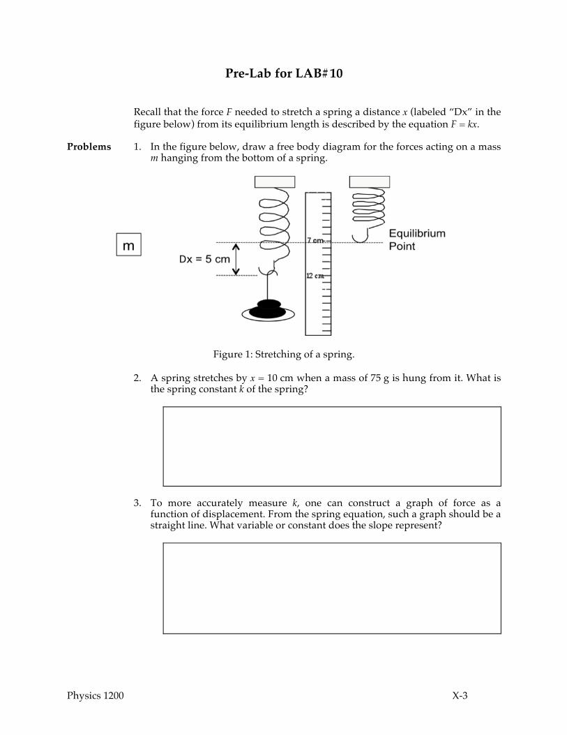
Recall that the force F needed to stretch a spring a distance x (labeled “Dx” in the

figure below) from its equilibrium length is described by the equation F = kx. Problems 1. In the figure below, draw a free body diagram for the forces acting on a mass

m hanging from the bottom of a spring.

Figure 1: Stretching of a spring. 2. A spring stretches by x = 10 cm when a mass of 75 g is hung from it. What is

the spring constant k of the spring?

3. To more accurately measure k, one can construct a graph of force as a

function of displacement. From the spring equation, such a graph should be a straight line. What variable or constant does the slope represent?

X - 4 Physics 1200

Pre-Lab for LAB#10

Problems 4. Below is a graph of displacement vs. time for an object that experienced

SHM. What is the amplitude of the oscillation of the motion? amplitude = ______ cm 5. Predict the ratio of the periods, T1 T2 , of two masses M1 and M2 = 4 M1 that

oscillate in SHM on springs that have the same spring constant k. Show the reasoning behind your prediction.

Physics 1200 X-5

Laboratory List of Today’s Activities Check Pre-Lab Introduction Introduction to the equipment. What is expected of students. Lab Activity Group Work and Concept Questions Lab Activity Measure the spring constant k Lab Activity Period versus amplitude for a spring Lab Activity Lab Challenge: Find the unknown mass. Activity 1 Group Work and Concept Questions Observe sinusoidal oscillations using the motion detector Use the motion detector to record the simple harmonic motion of a mass on a

spring. Observe the position, velocity, and acceleration graphs and discuss with your lab partners; then, answer the concept questions below.

Questions 1. A block on frictionless surface is connected to a wall by a spring. The

block oscillates between extremal points A and E. Identify the point(s) where each of the following is true: a. maximum speed: b. zero speed: c. maximum acceleration: d. zero acceleration:

2. Circle the direction of the force exerted by the spring on the block for the following situations:

X - 6 Physics 1200

Activity 2 Measure the spring constant k Record the equilibrium length of the spring with no additional mass attached.

Then measure the distance the spring is stretched when hanging a series of masses up to 170 g. Choose a reference point somewhere near the bottom of the spring or masses from which to record the differences. The displacement is the scale reading minus the reading for zero added mass.

IMPORTANT: The springs you are working with are quite delicate. Do not hang masses

greater than 200 grams from the springs, or they may be permanently stretched out of shape.

Table 1

Hanging Mass m

(kg)

Scale Reading x

(m)

Displacement Δx (m)

Stretching Force F = mg

(N)

0.000 0.000 0.000

0.050

0.080

0.110

0.140

0.170

Now open the LoggerPro template ‘Spring plot.cmbl’ on the desktop. Enter the

mass and displacement data into the worksheet. Do not include the point with zero hanging mass. LoggerPro will automatically generate a plot of stretching force F on the vertical axis versus displacement, Δx on the horizontal axis. LoggerPro can calculate the best linear fit to your data (click on the appropriate button near the top of the window). The slope of this line is the spring constant k.

k = ( ) include units!

Physics 1200 X-7

Activity 3 Period versus amplitude for a spring A mass m hanging on a spring with spring constant k oscillates with a period:

The mass m in this equation is the total mass, which includes the hanging mass, as well as the hook (30 g) and the spring itself (~1 g).

Note that the equation does not contain the amplitude (A) of the oscillation. Test

this relation by measuring the period of oscillation for a hanging mass of 120 g for several different amplitudes. To start the mass oscillating, pull the spring down by a few cm, then release. Use a stopwatch to record the time it takes the spring to complete 25 cycles of oscillation.

Table 2

Amplitude A

(cm)

Total time for 25 cycles 25T (s)

Period T (s)

Does the period depend on the amplitude? Compare the period measured above with the period calculated using the value

of the spring constant you determined above. Tmeasured = _______________ Tcalc = _______________ % difference = __________ f = 1/T = _______________ ( ) include units! Calculate the angular frequency of this motion: ω = 2π f = 2π/T = ________________ ( ) include units!

X - 8 Physics 1200

Activity 4 Lab Challenge: Find the unknown mass. Use the equation for the period of oscillation to find the mass of an object. unknown massspring = Use the scales in the lab room to measure the unknown mass. unknown massscale = Analysis How well did you do? Calculate the percent error to compare the two values of

the unknown mass: Error = (unknown massspring - unknown mass scale)/ unknown mass scale] x 100 = ____________ %


End of Lab 10

When you are finished, close Logger Pro. Do not save any changes.

Physics 1200 XI-1

Name ________________________________

Partner(s): ________________________________

Experiment 11: Introduction to Waves and Addition of Waves

Objectives Measure the period and frequency of sound waves Understand the addition of waves using the superposition principle, through

manifestations of two source interference, standing waves, and spectral analysis. Equipment Computer with LoggerPro and Labview, speakers, microphone, tubes, meter

stick Preparation You will be pressed for time during the lab. Since successful completion of all lab





XI - 2 Physics 1200

Pre-Lab for LAB#11

Intro A wave is a propagation of oscillations through a medium. At any point in the

medium through which a wave passes, the particles of the medium vibrate with simple harmonic motion (SHM) that has the same period, T, and frequency, f, as the wave. In a wave, the pattern of the displacement of particles of the medium from equilibrium repeats over regular intervals; such an interval is called a wavelength, λ. It is a characteristic of any wave that its frequency and wavelength are related to its speed, v, by

fλ = v Waves add when their paths cross. Under most conditions, the addition of

waves follows the principle of linear superposition, which states that the sum of two or more waves at a particular point in space and at a particular time is equal to the sum of the individual wave displacements. This principle is general to all types of waves; in this lab, you will study several aspects related to the addition of sound waves.

For example, standing waves result from the addition of two waves of the same

frequency and amplitude traveling in opposite directions. This situation often arises when waves reflect from boundaries, such as the closed or open ends of a tube. You can visit this website for an applet that will help you visualize this process:

http://www.walter-fendt.de/ph14e/stwaverefl.htm Problem Below is a record, displacement vs. time, of the oscillations of the particles of air

at a certain point that shows the SHM that resulted from a wave passing through that point. The period (T) is the time it takes a particle to complete one full oscillation. Calculate the period for the motion. For better precision and accuracy, try measuring the time it takes for more than one period of the oscillation, and then dividing by the number of oscillations to calculate the period.

Period = ________ s

Physics 1200 XI-3

Pre-Lab for LAB#11

Waves in air may be represented by oscillations of air molecules or of air

pressure. When representing standing waves in air, displacement nodes correspond to pressure antinodes (places of greatest pressure variation), and displacement antinodes correspond to pressure nodes (places of least pressure variation).

Problem Consider a pipe that is closed at one end. Sketch the standing wave pattern in

each of the following situations; showing the regions of high and low air pressure variations (pressure antinodes and pressure nodes). Then formulate equations that relate the wavelength λ and frequency f to the length L of the pipe.

a) Tube with one open end (“closed tube”): fundamental.

λ1 = f1 = b) Tube with one open end (“closed tube”): first overtone (3rd harmonic).

λ3 = f3 = c) Find the ratio of the first overtone and fundamental frequencies: f3/f1 = d) Tube with both ends open (“open tube”): fundamental.

λ1 = f1 =

e) Tube with both ends open (“open tube”): first overtone (2nd harmonic).

λ2 = f2 =

f) Find the ratio between fundamental and first overtone frequencies: f2/f1 =

XI - 4 Physics 1200

Laboratory

List of Today’s Activities Check Pre-Lab Introduction Brief review of key concepts and Pre-Lab questions Problem Solving Concept Questions Measuring frequencies of Sound: Lab Activity The frequency of sound – measuring the musical scale Standing Waves: Problem Solving Group Work Problem Lab Activity Measuring standing wave resonances in a tube Spectral analysis (aka Fourier analysis): Lab Activities Measuring the Fast Fourier Transform (FFT) of a single tone Beats - Adding waves with different frequency Comparison of piano and flute tones – musical ‘timbre’

FFT of a snap FFT of tube resonances

Lab Challenge none

Physics 1200 XI-5

Activity 1 Concept Questions

1. The schematics above illustrate the positions of molecules during the motion of two different sound waves through air at room temperature. Which wave:

- Has a higher frequency? A B Equal - Has a longer wavelength? A B Equal - Has a higher velocity? A B Equal

Using the scale given, estimate the wavelength in A. 2. The motion of one molecule at a moment in time is indicated by the arrow in A. The wave in A is moving: Right Left Can’t tell 3. Sketch below the horizontal position of this molecule as a function of time, averaged

over many wave cycles. You may want to consult this link: http://www.kettering.edu/~drussell/Demos/waves/wavemotion.html

XI - 6 Physics 1200

Activity 2 Measuring Sound Frequency The common Tempered Scale divides our audible range into a series of octaves,

each of which is divided into 12 intervals; because of this, each successive note is 212 times the previous note. On a piano, these are the 7 white keys and 5 black

keys. Your instructor will play a series of notes on an electronic keyboard. Open the LoggerPro template ‘microphone.cmbl’, which will allow you to monitor your microphone’s response as each note is played. Start the program by clicking on the green ‘Collect’ button at the top of the window. Your microphone is operating correctly if you see background noise on the screen. You and your partner(s) will each measure the period of a note, and then average your results. By measuring the period of the microphone signal, you can calculate the frequency, f, of each note (i.e. the note’s “pitch”).

Period = T frequency = 1/T Your instructor will play the notes of the scale using the setting Flute: 13. Each group will measure a different note, so that the class as a whole will be able

to fill in the following table.

Note Period (s) Frequency (Hz) Accepted freq (Hz)

C4 (4th octave) 261.63

C# 277.18

D4 293.66

D# 311.13

E4 329.63

F4 349.23

F# 369.99

G4 392.00

G# 415.30

A4 440.00 (exactly)

A# 466.16

B4 493.88

C5 (5th octave) 523.25

Physics 1200 XI-7

Activity 3 Group Work Problem – Schumann resonances (Earth’s standing waves)

Radio waves can reflect off a layer of the atmosphere called the ionosphere, where a large portion of the atoms and molecules has been ionized by solar UV. Radio waves can also reflect off the Earth’s surface. In effect, radio waves bounce back and forth off the surface and ionosphere, just as visible light can bounce between two metal mirrors. Lightning and other natural phenomena generate radio waves with a range of frequencies. Those frequencies that are just right will travel around the earth, meet themselves in phase, and form standing waves. The set of frequencies that will do this are known as Schumann resonances, in honor of Winfried Otto Schumann (1888-1974, Germany), who predicted their existence in 1952.

In this exercise you will estimate the first 5 Schumann resonances using what you know about standing waves. The picture below illustrates the standing wave pattern for one of the resonances. Keep in mind that the atmosphere is really just a thin skin surrounding the Earth, so that the waves really circle the Earth at close to the Earth’s radius, which is re ~ 6378 km.

1) How many wavelengths fit around the loop

in this picture?

2) What is the wavelength?

λ = ( ) units?

3) Write a general equation for the standing waves:

nλ = Using this equation, fill in the following table. Compare your calculated

frequencies (fcalc) with the observations (fobs) at: http://www.glcoherence.org/monitoring-system/earth-rhythms.html

resonance wavelength (km)

fcalc (Hz) fobs (Hz)

1

2

3

4

5

XI - 8 Physics 1200

Activity 4 Standing waves in a tube In this Activity you will use a microphone to directly measure the standing wave resonances in an open ended tube and compare this to calculated values. Set the microphone near the speaker, and open the LoggerPro template ‘microphone.cmbl’. This program allows you to directly monitor a microphone’s output as a function of time. First, run the program by clicking on the green ‘Collect’ button. You should see the microphone’s output on the screen as it picks up background noise from the room. Now open the Labview program ‘output sound.vi’, which will allow you to generate a single tone from the laptop’s speakers. To run the program, hit Ctrl-R, or the right arrow button at the top of the window. To stop, hit Ctrl-. or one of the stop buttons at the top of the window. You can adjust the sound frequency by clicking on the slider control, or by using the digital indicator. Verify that the microphone output is a clear sinusoidal signal. Place your speaker at one end of the plastic tube, and the microphone at the other end. Adjust the volume to be as low as possible, while still producing a clear signal on the computer. This will minimize interference with neighboring groups (and prevent headaches). You can adjust the horizontal and vertical axes as needed.

Vary the frequency between 0-1000 Hz as you monitor the microphone’s output on the computer. You can precisely adjust the frequency by using the digital indicator on the tone generator program. At one or more ‘resonant’ frequencies within this range, standing waves are formed, and the microphone output should be particularly large. The process is similar to blowing gently over a soda bottle, where for certain conditions, a pronounced sound is heard. If you don’t notice any values where the microphone output is larger, try varying the frequency over this range more slowly. The lowest frequency resonance you can pick out is likely to be the tube’s fundamental frequency. Estimate how precisely you can locate the fundamental frequency, by having your partner(s) repeat the process. Fundamental frequency = _____________ Error estimate = ± _______ When you have precisely identified the fundamental frequency, record this value in Table 1 and repeat this process for the next 3-4 resonances. The higher resonances may be more difficult to identify. To accurately predict the resonance frequencies for comparison, it is necessary to make an end correction, which compensates for the fact that the vibrating air column extends slightly beyond the two ends of the tube. As a result, the tube has an effective length, Leff , given by: Leff = L + 2 × 0.3× d , where L is the measured length of the tube, and d is the diameter. Record these values in Table 1, and calculate Leff.

Physics 1200 XI-9

Now calculate the standing wave frequencies for your tube (fn calc in Table 1). Use the equations you derived in the PreLab, and take Leff as the length of the tube. Use 434 m/s as the speed of sound. Enter these values in Table 1.

TABLE 1

Resonance # fn (Hz) Ratio: fn / f1 fn calc (Hz) Percent error = |fn- fn calc |/ fn calc

n=1 f1/f1 = 1

2 f2/f1 =

3 f3/f1 =

4 f4/f1 =

5 f5/f1 =

Compute the ratio of measured resonance frequency, fn , to the measured fundamental frequency, f1. Does the ratio fn/f1 follow the pattern you expect from the PreLab? Why or why not?

Were your measured frequencies close to your calculated values? Why or why not?

Have your instructor check your work before you proceed.

L = d = Leff =

XI - 10 Physics 1200

Activity 5 Spectral Analysis The human brain/ear system is a remarkable instrument. Sounds with intensity spanning 12 orders of magnitude can be detected, allowing us to hear soft whispers one minute, and jet engines the next. The brain/ear system also performs spectral analysis of sounds in real-time. This ability allows us to pick out individual instruments in a symphony, and eavesdrop on a conversation in a crowded room. This Activity will introduce you to some concepts related to spectral analysis. The Fast Fourier Transform (FFT): The FFT of a signal produces a spectrum, which is a plot of amplitude versus frequency. Any time-domain signal f (t) can be represented as the sum of sine waves with different frequency (cosines are simply shifted sine waves):

The more complicated the signal, the more sine waves are needed. It is often convenient to view the frequency spectrum of complicated signals, which essentially is a plot of the coefficients an, bn as a function of frequency. The process of calculating these coefficients from f (t) is known as a Fourier transform. The “fast Fourier transform” is a convenient algorithm for performing this calculation using your computer. You will use Logger Pro to calculate the FFT frequency spectrum of familiar sound waves. FFT of a single tone: A pure sine wave tone has the simplest FFT, because only one sine wave in the Fourier series is required. Load the LoggerPro template “FFT.cmbl”. You will see two graphs: one is the time domain signal picked up by your microphone, the second is the calculated FFT frequency spectrum. Position your microphone near the speaker (the tube is not needed for this part), and set your computer to output a tone with frequency between 100-1000 Hz. Run the LoggerPro program by clicking on the Collect button. Sketch what you see in the two panels: Time domain Frequency domain

Check that the FFT signal corresponds to the frequency output: Output frequency = _________ ( ) FFT peak = ______________ ( )

Physics 1200 XI-11

Activity: Beats (adding waves with different frequency) Activate the second output in the Labview program ‘output sound.vi’. You can now output two sine waves at the same time. Set one of the frequencies and adjust the other to match. As the two frequencies begin to match, you will hear a slow modulation in amplitude. This is called a beat phenomenon. Measure the spectrum using the LoggerPro FFT program, and sketch the time and frequency domain signals you observe. For clarity, the two frequencies should differ by more than 4 Hz. Be sure to adjust the axes in the graphs to clearly observe the beats in both domains. Time domain Frequency domain

Measure the beat period in the time domain signal: T beat= __________ ( ) Record the frequencies: f1 = __________ ( ) , f2 __________ ( )

Now compute the expected beat period: Tcalc =1

f2 − f1= ___________ ( )

Do the numbers match? Beat phenomena provide a useful way to measure the frequency of unknown signals. With the Labview program running, have a partner set one of the output frequencies to an unknown value, and toggle the switch to hide the slider. You can now indirectly measure this frequency by tuning the frequency of the first output until you hear very slow beats. How close did you get? Matching frequency = __________ ( ) ‘Unknown’ frequency = _________ ( ) Switch roles with your partners until everyone has had a chance. This is an example of “heterodyne” detection, which is widely used to detect high frequency signals in electronics. Musical ‘timbre’ (comparing a piano and a flute): How do we tell the difference between a piano and a flute? Musical notes played on real instruments are not pure sine wave tones like you’ve been using today: they also contain additional harmonics. You will find two mp3 files on your desktop that contain examples of the same note played on a piano and on a flute. To compare the spectrum of each instrument using the LoggerPro FFT program, you first need to activate the trigger function by clicking on the “Data Collection” button just to the left of the green Collect button. On the Collection tab, set the length to 0.06 s, and on the Triggering tab, enable triggering on a sensor value that is ~ 0.03 au larger than the background noise level


picked up by the microphone (this number appears in the bottom left corner of the window). After setting these values, exit the dialogue box. Now when you click the green Collect button, the program will wait for a trigger.

Play an mp3 file to trigger the data collection, and sketch the FFT spectra from 100-2kHz: Piano

Flute

What is different between the two sets of spectra? Which note is being played? (you may want to refer to Lab 11) Note = __________

Physics 1200 XI-13

FFT of a complicated signal: Now trigger data collection with a sharp impulse of sound, such as that produced when you snap your fingers or clap your hands. Many more sine wave components are present in such a complicated signal. As a result, the FFT shows a spectrum that extends over the whole range of human hearing (and beyond!). Sketch what you see in the two panels from 100-20kHz: Time domain Frequency domain

Activity: FFT of tube resonances Now that you have successfully measured the standing wave resonances of a tube the hard way, you can use the FFT to do the same measurement much more quickly. As you’ve seen, a continuum of sine waves is generated when you snap your fingers. Frequencies within this continuum that correspond to standing wave resonances will be preferentially transmitted through the tube. Position your microphone at one end of your tube. Trigger data collection by snapping your fingers (or clapping your hands) at the other end of the tube. The FFT should show a series of peaks at the tube’s resonant frequencies. You may need to repeat this a few times to get clear peaks in the FFT. Record the frequencies fn FFT in Table 2, and compare these values with those you measured (fn) and calculated (fn calc) earlier (Table 1).

Table 2 Resonance # f n FFT (Hz) f n (Hz) fn calc (Hz)

n = 1

2

3

4

5


Do your values agree? If not, speculate on what could cause any discrepancies. This is an example of Fourier Transform spectroscopy, which is widely used in modern infrared spectrometers (FT-IR) and nuclear magnetic resonance (NMR and MRI). These techniques have applications throughout the physical and life sciences.


End of Lab 12 When you are finished, close both LoggerPro and Labview. Do not save any changes Handy links: Fourier synthesis applet: http://www.falstad.com/fourier/ End corrections in wind instruments: http://www.phys.unsw.edu.au/jw/musFAQ.html#end Flute acoustics: http://www.phys.unsw.edu.au/jw/fluteacoustics.html Basics of digital filtering: http://www.falstad.com/dfilter/

Physics 1200 B-1

Appendix B

Introduction to LoggerPro

To start data collection, click the green “Collect” button on the tool bar. There is a delay of a second or two before data collection starts, so don’t try to time clicking the button with your actions. Many parameters in the software are adjustable, like the sample collection time. Adjusting them is done through the menus, but some common commands and parameters are available through the toolbar. For example, click the clock icon to change the sample rate or time. Often you will be told to load/open a file. Such files will set all the relevant parameters for the experiment. Graph parameters can be changed by clicking on the graph to select it and using the menus, or by right-clicking on the graph. Common graph commands include zoom and autoscale. Note that LoggerPro typically measures position-like variables and calculates derivatives like velocity and acceleration. If LoggerPro crashes restart the program and re-open the last initialization file used. Any changes you may have made to LoggerPro’s configuration by hand will have been lost and will have to be re-performed if desired. If you can’t see your data (the graphs appear blank) or the data is a flat line at zero you probably need to adjust the graph scaling. Start with “Autoscale from 0”, then zoom-in or adjust the axes. If the data look good at first but suddenly become choppy or weird while using the position detector the object you are measuring has probably moved outside the detector’s measurement cone. If this is a cart & track experiment, try adjusting the hinge of the detector. The sensor might be tilted too far back. If the “collect” button is gray and can’t be clicked then there may be a problem with the sensor hardware. Make sure the cable to the sensor is snapped in place

Sensor setup w

indow

Data Brow

ser

Autoscale

Set data collection param

eters

Start/Stop collection

Define zero

Open file

B - 2 Physics 1200

and likewise with the cables going to the interface box. (The cable from the sensor goes to the interface box; just follow it.) If the button is still gray, the problem might be the software. Quit out of LoggerPro and restart it. If all else fails, ask your lab instructor for help.

Physics 1200 C‐1

Appendix C

Equipment for Laboratory Experiments Experiment 9: Fluids Force Probe Venturi Tube Experiment 10: Simple Harmonic Motion Spring Ruler Weight hanger Hook Masses Timer Motion detector Experiment 11: Introduction to Waves and Addition of Waves Computer with LoggerPro and Labview Speakers Microphone Resonance Tubes Meter stick

physics 1210 lab manual 1210 laboratory manual ... the water’s speed at 25.0 m/s. at point b, ......

Documents