WP 16/22

Physician Group Practices and Technology

Diffusion: Evidence

from New Antidiabetic Drugs

Kathleen Nosal

August 2016

http://www.york.ac.uk/economics/postgrad/herc/hedg/wps/

Physician Group Practices and Technology Diffusion: Evidence

from New Antidiabetic Drugs

Kathleen NosalThe University of Mannheim

May 24, 2016

Abstract

One way that physicians learn about new treatments and technologies is through interactions withother physicians. Such interactions are shaped, in part, by the structure of group medical practices:physicians who work in the same practice have more opportunities to exchange ideas. To quantify theimportance of physician practices in technology adoption, I analyze physicians’ adoption of three newanti-diabetic drugs introduced between 2009 and 2011 using data on the universe of Medicare Part Dprescriptions. I construct the network of colleague relationships through practice memberships, andtest whether physicians are more likely to adopt the new drugs if they have colleagues who do so. Todistinguish the causal effect of interest from other sources of correlated decisions within practices,I use instrumental variables and also a panel data approach with physician and drug fixed effects.The instruments exploit the network structure, using characteristics of second degree connections(colleagues of colleagues) as a source of exogenous variation. The results indicate that having acolleague who prescribes the drug is associated with a 21 percentage point increase in a physician’sprobability of adopting the drug, compared to a 2 to 5 percent baseline adoption probability.

1 Introduction

Each year the U.S. Food and Drug Administration (FDA) approves several dozen new prescription

drugs to go on the market. For example, in 2015 the number of new drug approvals was forty-five.1

In order to obtain FDA approval, the applicant must demonstrate that the drug has clinical benefits

that exceed the risks for some category of patients. However, there is an additional barrier, beyond this

approval process, before patients can benefit from a drug: physicians must begin prescribing it. Learning

about new drugs is a non-trivial information investment for physicians. A large literature describes how

physicians learn about the safety, efficacy, and patient match value of drugs through within-patient

experience (Crawford and Shum, 2005), across-patient experience (Berndt, Pindyck and Azouley, 2003),

detailing by pharmaceutical representatives (Ching and Ishihara, 2010) and academic and media articles

(Chintagunta, Jiang and Jin, 2009.)

This paper is concerned with a particular aspect of physician learning about new drugs: peer effects

among colleagues in physician group practices. I quantify the effect of colleagues’ adoption decisions on a

physician’s probability of adopting a new drug. The idea is that physicians who work in the same group

practice have many opportunities to interact, leading to information spillovers about new drugs. These

1The FDA provides information about newly approved drugs online athttp://www.fda.gov/Drugs/DevelopmentApprovalProcess/DrugInnovation/default.htm

1

spillovers can make it less costly for additional physicians in a practice to adopt a drug once someone

has already done so.

The focus of this paper is on physician adoption of three new antidiabetic drugs that came onto

the market between 2009 and 2011: Onglyza, Victoza, and Tradjenta.2 I combine physician-drug-level

prescribing data from Medicare Part D3 with another Medicare data set which has information about

group practice membership. In several econometric specifications, I then test for an effect of group

practice colleagues’ prescribing decisions on whether a given physician begins prescribing the drug.

There are well-known econometric challenges involved in measuring peer effects, as described by

Manski (1993) and Moffit (2001). The reflection problem refers to the difficulty in distinguishing between

the effect of the peer group on the individual, and the effect of the individual on the peer group.

Additional endogeneity problems arise when peer groups are formed endogenously, raising the possibility

that sorting on observed and unobserved characteristics leads to spuriously correlated outcomes.

To address these endogeneity problems, I follow the approach of Bramoulle, Djebbari and Fortrin

(2009) and Di Giorgi, Pellizzari and Redaelli (2010). Both sets of authors point out that the reflection

problem can be solved when peer groups are partially, but not completely, overlapping. In my setting,

many physicians work at multiple practices. The physicians that a given physician works with in the same

practice (possibly across multiple practices) are the physician’s direct peer group, which I refer to as first-

degree colleagues. Physicians also have indirect peers, or second-degree colleagues. These are first-degree

colleagues of first-degree colleagues, who are not directly connected to the focal physician. Bramoulle

et al. and Di Giorgi et al. point out that these indirect connections help with identification. First,

partially overlapping peer groups imply that there is variation in peer groups even across individuals

who are peers. Second, a natural instrument emerges: characteristics of second-degree colleagues. These

characteristics satisfy the exclusion restriction because they are not part of the focal individual’s direct

environment, as characteristics of first-degree connections would be, but are relevant because they can

affect the focal individual through the common peers.

In addition to using the second-degree colleague instruments, I also control for physicians’ own char-

acteristics, and characteristics of their first-degree colleagues. The control variables include measures

of the physician’s previous prescribing history with drugs in the same therapeutic class and with drugs

marketed by the same pharmaceutical firm, with the intention of proxying for the physician’s patient mix

and exposure to drug-specific promotional activity. I also estimate a panel data model, pooling the data

2Onglyza, Victoza, and Tradjenta are all drugs that improve the glycemic control of adult patients with Type 2 diabetes.Onglyza has the generic name saxagliptin and is taken orally. It was introduced in July 2009. Victoza has the generic nameliraglutide and is an injectable. It was introduced in January 2010. Tradjenta has the generic name linagliptin and is takenorally. It was introduced in May 2011. All three were under patent protection for the duration of the sample period. Aboxed warning was issued for Victoza in March of 2015 because of its role in causing thyroid tumors. Because this is threeyears past the end of the sample period, I assume that the boxed warning has no effect on observed adoption decisions.

3Medicare Part D is the arm of Medicare which provides prescription drug coverage to the elderly. For the purposesof this data set, Medicare Part D refers to both standalone Medicare Part D plans, and drug coverage obtained throughMedicare Part C managed care plans.

2

across the three drugs and allowing for drug and physician fixed effects. This specification, combined

with the second-degree colleague instruments, is meant to control for endogeneity caused by correlated

unobserved characteristics as well as the endogeneity related to the reflection problem.

Physician group practices legally can take different forms, but generally refer to two or more physicians

working in a common office and often sharing administrative or other resources. Over time, group

practices have become more prevalent in comparison to solo practices, and the average size of group

practices has been growing (Welch et al., 2013). Recent literature has stressed the importance of physician

group practices for understanding market power and competition in the market for physician services

(Dunn and Shapiro, 2014; Baker et al. 2014; Town, Feldman and Kralewski, 2011). Less attention has

been paid to how this aspect of market structure affects interaction between physicians, and the resulting

consequences for patient care.

This paper fits broadly into the large literatures on peer effects (e.g., peer effects in education, surveyed

by Epple and Romano, 2011) and technology diffusion in social networks (e.g., Conley and Udry, 2010).

More specifically, there is already a small literature on peer effects in physician prescribing. Indeed, one

of the seminal papers in sociology on social network analysis studies the diffusion of an antibiotic among

physicians in four cities (Coleman, Katz and Menzel, 1957). More recently, Nair, Manchada and Bhatia

(2010) study the role of “opinion leaders”, or research-active specialist physicians, in influencing their

peers to adopt new drugs in an unspecified therapeutic class. My paper differs from this prior work in

at least three ways. First, the way that I define peer groups is fundamentally different. Both Coleman

et al. and Nair et al. use self-reported connections from survey data to establish connections between

physicians, while I use membership in group practices. In addition to avoiding the shortcomings of survey

data, I address a different question, about the interplay between market structure and information flow.

Second, I use a different identification strategy than Nair et al. that is more robust to multiple sources of

endogeneity.4 Nair et al. use a panel data approach to control for physician fixed effects, but I go a step

further and use instruments based on characteristics of excluded second degree colleagues. My approach

is designed to tease out the causal relationship even in the presence of simultaneity of decision making

and correlated effects at the peer group level. Third, I use a much more comprehensive data set, making

external validity more plausible. My data covers nearly all physicians with patients enrolled in Medicare

Part D, which amounts to over 600,000 physicians. Nair et. all and Coleman et al. use small samples

of physicians that participated in surveys– 1500 and 125 physicians respectively. These samples simply

aren’t as nationally representative as mine. Two other papers are closely related in some dimension.

Saxell (2014) also addresses learning spillovers between physicians, but is interested in the effect within

a given patient. In her paper, physicians can learn about the match quality between a patient and

4Of course, Coleman at al., as sociologists working in the 1950s, were not very concerned with endogeneity at all andwould not have had modern econometric tools to control for it even if they were. This is all the more excusable becausetheir paper was so far ahead of its time in other respects. Therefore, I focus on the contrast with Nair et al. here and leaveColeman et al. alone!

3

drug from previous prescriptions from a different physician. Karaca-Mandic, Town, and Wilcock (2016)

study the impact of hospital and physician market structure on the diffusion of cardiac stents. They are

primarily interested in the effect of measures of competition on technology adoption, so the mechanism

is quite different from the one in the current paper. In a 2005 survey paper, Manchada et al. point to

the many open questions about the role of peer effects in prescribing behavior. This paper contributes

to answering some of those questions.

2 Model

In this section, I describe the model. In the first subsection, I establish how colleague relationships

are defined in terms of network connections through group practice memberships. In the subsequent

subsections I describe the econometric specifications to be estimated, beginning with a simple linear

probability model, and building up to instrumental variables and panel data specifications which address

the endogeneity and reflection problems.

2.1 Colleague Definitions

A major building block of the model is “colleague” relationships through practice memberships. First-

degree colleagues work together in the same practice. Second-degree colleagues have a colleague in

common, but do not themselves work together. To formalize this idea, let i index physicians, and let p

index practices. Let cip equal 1 whenever physician i is a member of practice p and equal 0 otherwise.

Physician i’s set of first degree colleagues is defined as follows:

G1i ≡ {i′ : ∃p : cip = ci′p = 1} (1)

The definition simply states that for i′ to belong to the set of i’s colleagues, there should exist a practice

where both are members. Recall that physicians can belong to multiple practices, so that cip = 1 and

cip′ = 1 are not mutually exclusive. Therefore, it can be the case that i′ ∈ G1i and i ∈ G1

i′ but G1i 6= G1

i′ .

These non-fully-overlapping sets of first degree colleagues is what allows for the existence of second degree

colleagues. If physicians i and i′ are colleagues, there can still be a member of G1i′ who is not a member

of Gi. Such a physician would be a second degree colleague of i. The set of i’s second degree colleagues

is defined as:

G2i ≡ {i′′ : ∃i′ : i′ ∈ G1

i , i′ ∈ G1

i′′ , i′′ /∈ G1

i } (2)

4

2.2 Basic Model

Let d index the three drugs, and let td denote the second full year that the drug is on the market.5 The

first specification is a cross-sectional model of adoption of drug d at time td, run separately for each drug.

Let yid be an indicator that is 1 if physician i has adopted drug d in period td. Exogenous physician

characteristics xid are partitioned into two sets: characteristics x̃i which vary only by physician, and

characteristics x̃id which vary by both physician and drug. The estimation equation is:

yid = α+ β maxi′∈G1

i

{yi′d}+ γxid + δE(xi′d|i′ ∈ G1i ) + uid (3)

The parameter β is the peer effect of interest, measuring the effect of having at least one colleague

who adopts the drug on the physician’s own adoption choice.6 The parameter vector γ captures the

effect of the physicians’ own characteristics, including those that are drug-specific, and δ controls for

mean characteristics of colleagues. In the peer effects literature, β is referred to as an endogenous peer

effect, while δ is a vector of exogenous peer effects.

Simply estimating equation (3) by OLS will not yield consistent estimates of the parameters, due to

endogeneity. In particular, maxi′∈G1

i

{yi′d} is likely to be correlated with uid both because of non-random

sorting into practices with respect to uid, and the potential for reverse causality between yid and each

yi′d in G1i . These limitations motivate the instrumental variables and panel data specifications described

below.

2.3 Instrumental Variables

Instruments are needed which are correlated with the endogenous colleague outcome maxi′∈G1

i

{yi′d} but not

with the error term uid. A natural candidate is mean characteristics of second degree colleagues:

zid = E[xi′d|i′ ∈ G2i ] (4)

Any subvector of zid can be used as instruments. The endogoneity problem that is being addressed is

that each yi′d is potentially an outcome of physician i’s adoption decision instead of a cause of it, because

in an environment with spillovers all the adoption decisions are interrelated. Physician and physician-

drug characteristics xid do not suffer from this problem because they are predetermined with respect to

the adoption decisions. However, the physician’s own characteristics, and the average characteristics of

the physician’s first-degree colleagues already appear in the main equation, because they may directly

5For example, Onglyza was introduced in 2009, so tonglyza = 2011.6In the peer effects literature, it is more conventional to use the average decision across colleagues rather than the

indicator used here. I use this version of the variable because it makes the results easier to interpret in this context. Withthe median physician having zero colleagues who adopt, it is not clear how to turn the coefficient on average adoption intoa meaningful marginal effect.

5

affect the physician’s adoption decision. The average characteristics of second-degree colleagues, on the

other hand, are excluded from the main equation. These average characteristics do not directly affect

physician i, as they are not part of the common practice environment like the characteristics of the

first-degree connections. The effect of these characteristics should come through the mutual first degree

colleagues, which is how the relevance condition for the instruments is satisfied.

Using instruments of this type is the solution to the reflection problem suggested by Bramoulle,

Djebbari and Fortrin (2009) and De Giorgi, Pellizzari and Redaelli (2010). Their papers provide a

formal derivation of how non-overlapping peer groups lead to a set of exclusion restrictions that justify

using the second degree peers characteristics as instruments.

Unfortunately, the IV approach doesn’t fully solve the endogeneity problem in this case. Since

practices are formed endogenously, physicians’ observed and unobserved characteristics may be correlated

(positively or negatively) with those of colleagues within the same practice. As a result, the composition

of a physician’s second degree colleagues is not exogenous with respect to the physician’s unobserved

characteristics. To address this concern, I estimate a panel data model.

2.4 Panel Data Model

The panel data model pools data across the three drugs, and uses within-physician, across-drug vari-

ation in colleague adoption rates to identify the effect of interest. The data pooling is done such that

observations for each drug are taken from the second full year in which that drug was on the market, as

in the previous model.

The panel data specification includes drug and physician fixed effects. The drug fixed effects are

meant to capture the differential popularity of the drugs that affects all physicians equally. For example,

the three drugs could differ in the proportion of the population with diabetes for which they are suitable,

or could have differing levels of advertising. The physician fixed effect is meant to capture the part of

physician heterogeneity which affects the physician’s adoption probability for any of the three drugs.

For example, some physicians could simply be better informed about new drugs in general, or some

physicians could have more patients with diabetes or a stronger tendency to choose drugs as a course of

treatment.

The subset of the physician characteristics that vary at the physician-drug level, x̃id, are included

as controls, along with the mean across first degree colleagues of these variables. In practice, these are

variables which measure the physician’s past experience with other drugs from the same pharmaceutical

firm as drug d (details are in the data section.) The other control variables from the previous specification

are supplanted by the physician fixed effects.

6

The estimating equation is:

yid = β maxi′∈G1

i

{yi′d}+ γx̃id + δE(x̃i′d|i′ ∈ G1i ) + λi + κd + uid (5)

2.5 Panel Data with Instrumental Variables

To address both endogeneity concerns at the same time, the instrumental variable and panel data ap-

proach can be combined. In fact, this two-pronged approach has been used in other applications with

partially overlapping peer groups that are endogenously formed (Di Giorgi, Frederiksen and Pistaferri,

2013 and Claussen, Engelstaetter and Ward, 2014).

Using instruments in the panel data setting comes with an additional requirement. The instruments

must vary at the physician-drug level in order to be linearly independent from the fixed effects. As

before, characteristics of second degree colleagues are used to form the instruments, but in this case only

those that also vary by drug:

z̃id = E[x̃i′d|i′ ∈ G2i ] (6)

A subvector of z̃id is used to instrument for maxi′∈G1

i

{yi′d} in equation (5).

3 Data

Two data sources are joined to construct the data set used in estimation: one containing physician-level

prescribing information, and another containing physician characteristics and practice membership.

3.1 Data Sources

The prescribing data is from Propublica’s Medicare Part D Prescribing Data sets from 2010-2013. Prop-

ublica obtained the data from Centers for Medicare and Medicaid Services (CMS) through a Freedom

of Information Act request.7 CMS constructed the data from the universe of Medicare Part D prescrip-

tion drug claims. These claims represent prescriptions filled by the approximately 30 million enrollees in

standalone Medicare Part D prescription drug plans or Medicare Advantage plans with prescription drug

coverage. The data is aggregated at the level of physician and drug. Whenever a physician wrote 11 or

more prescriptions that were filled for a drug in the given year, there is an observation for that drug and

physician. The name of the drug, number of claims (including refills) and administrative identifiers for

the physician are given. Claim counts of 10 or fewer are suppressed, so absence of a physician-drug pair

in the data can either mean that the physician did not prescribe the drug at all that year, or that the

provider prescribed the drug 10 or fewer times. Each year’s data contains over 20 million physician-drug

7Propublica is an investigative journalism non-profit. The data sets are available for download athttps://projects.propublica.org/data-store/, except for the 2013 data which is available directly from the CMS.

7

observations.

The physician practice and characteristics data is from the Medicare Physician Compare database

obtained from CMS in 2013.8 The data covers every physician who had Medicare Part B claims in a given

time period. The data lists the group or solo practices that the claims were processed through. Some

practices have multiple locations, which are distinguished in the data by the practice street address. A

physician may have claims through one or more practices, and one or more locations within a practice.

There is an observation for each physician-practice-location combination, associating each physician with

every practice location where she had claims. This feature of the data is what allows me to construct

the network of colleague relationships, based on linking physicians who have claims at the same practice

and location. The data also includes physician characteristics, such as the physician’s specialties, gender,

and medical school graduation date.

The Physician Compare data provides a snapshot of practice membership in 2013, while prescribing

is observed in each year from 2010 to 2013. It would be ideal to observe the Physician Compare data in

each of these years, but CMS does not make this earlier data available. Over time, physicians presumably

move, switch practices, open new practices, and retire. As long as these changes are gradual, the 2013

data should provide a reasonable approximation to the configuration of practice memberships in 2010-

2012. However, the timing mismatch likely introduces some extra noise.

3.2 Network Data

The network of colleague relationships is constructed using the Physician Compare data, based on prac-

tice membership to determine who works together. I use both the practice identifiers and the address

information in the data to assign physicians to practices. The data identifies practices with a name and

unique practice number, but these identifiers are based on practices as an administrative entity rather

than a group of physicians working together at a particular location. Many practices are associated with

multiple addresses, and some even have addresses in multiple cities or states. While these locations are

administratively linked in the claims data, physicians at different locations of the same practice do not

work together in the sense that is of interest for this paper, even if technically they are employed by

the same firm. Therefore, the relevant unit of observation is a practice-location, a unique combination of

practice identifier and address.9

Once practice memberships are established, then constructing the colleague network is simple. Any

two physicians who belong to the same practice-location are linked. Some physicians work at multiple

practice-locations (either within the same practice or across practices), and thus have colleagues from

8The Center for Medicare and Medicaid Services posts the most recent version of the Medicare Physician CompareDatabase for download at https://data.medicare.gov/data/physician-compare.

9In order to avoid erroneously identifying distinct practice locations based on minor spelling variations of addresses, Iuse fuzzy matching techniques, so that addresses that differ by only a few characters are considered to represent the samelocation.

8

multiple practice-locations, who may be distinct or may have some overlap. Multiple practice membership

is what allows for the existence of second-degree colleagues. A second-degree colleague is a colleague of

a colleague, who is not also a colleague. For example, if physician 1 and physician 2 work together at

practice A, and physician 2 and physician 3 work together at practice B, then physician 1 and physician

3 are second-degree colleagues. Second-degree relationships are important for the construction of the

instruments.

About 18% of physicians in the data work only at solo practices and therefore have no colleagues.

These physicians are excluded from the analysis, because it makes no sense to measure the impact

of colleague’s prescribing behavior for someone who has no colleagues. Two types of outliers are also

removed from the data: physicians with unusually many practice memberships, and practices with

unusually many physicians. I remove physicians with more than 15 practice memberships, which is

about 0.2% of the physicians in the data. Such observations are likely a result of some kind of mistake in

the data, but even if a physician truly does work at 15 different practices, it is unlikely that she spends

enough time at each practice to influence colleagues at all of them. For practices, I set the cutoff at 150

physicians. Approximately 1% of practices have more than 150 members and are thus removed from the

data. When a practice is removed from the data, this means that no physicians are linked as colleagues

through that practice, but the associated physicians remain on the data and can be linked through other

practices. Some of the entities identified as practices in the data are actually hospitals, rather than

medical practices as such. Eliminating very large practices reduces the number of these hospitals that

remain in the data (though, perhaps some legitimate large practices are lost as well.) Table (1) shows

summary statistics about practice and colleague connections based on the data with the modifications

described above. The middle 50% of physicians work at 1 to 2 practice-locations and have between 6

and 60 colleagues. The middle 50% of practice-locations have 2 to 8 physicians.

Of physicians who survive the sample restrictions above, 78% have at least one second degree col-

league. Second degree colleagues are crucial to the identification strategy, and are used to construct

the instruments. Since the instruments are undefined for physicians without second degree colleagues,

such physicians are omitted in the main analyses reported in this paper. Of course, this could introduce

selection bias if, for example, the physicians without second degree colleagues work at fundamentally

different sorts of practices than those with. To explore the implications of this selection bias, I have also

run some estimations where I leave the physicians without second degree colleagues in, and set their

instrument values to zero. In general this affected magnitude of coefficients, but usually not signs or

significance.

9

3.3 Data Join

The prescribing data is linked to the Physician Compare data based National Provider Identifiers (NPIs).

The NPI is a 10-digit number assigned to each physician by CMS as a uniform identifier used across

multiple data systems. Unfortunately, while every observation in the Physician Compare data has an

NPI, the prescribing data suffers from some missing NPIs in cases where a different administrative

identifier is used instead. Since observations without an NPI cannot be associated with a particular

physician in the Physician Compare data, these observations are dropped from the data. This affects

only about one percent of physician-drug observations.

There is also the question of whether the physicians from the two data sources should perfectly

coincide, given that the data come from two different programs within Medicare. The Physician Compare

data is derived from billing data from Medicare Part B, the single-payer outpatient health insurance

component of Medicare. The prescribing data is from Medicare Part D, which encompasses standalone

prescription drug plans which Part B enrollees are eligible for, as well as drug coverage for Part C

enrollees as part of managed care plans chosen instead of Part B coverage. Physicians treating patients in

standalone Part D plans would definitely be in the Medicare Compare data, but if a physician exclusively

treats Part C patients, he might appear in the prescribing data but not in the Physician Compare data.

Fortunately, the number of unmatched observations is small.

3.4 Dependent Variable and Main Explanatory Variable

The dependent variable is an indicator for whether the physician has adopted the new drug. The

indicator is set to one whenever the physician-drug combination exists in the prescribing data. Of

course, the accuracy of this adoption indicator is subject to the data limitation that a drug-physician

combination is only observed if more than 10 claims were recorded. This limitation effectively creates

a threshold: the physician is only considered to have adopted the drug if she prescribes it at least 11

times.

In the main specifications, the explanatory variable is an indicator for whether the physician has

at least one first-degree colleague who adopts the drug. This is formed by taking the maximum of

the adoption indicators across the physician’s set of first-degree colleagues. For robustness checks (not

reported here), I form additional measures of colleagues’ adoption decisions. These additional variables

are the adoption rate (the mean of the adoption indicator across colleagues) and the adoption count (the

sum of the adoption indicator across colleagues.)

10

3.5 Control Variables

The physician level control variables are years in practice, a male-gender indicator, specialty indicators,

number of colleagues, number of practice-locations, and variables describing the portfolio of drugs in

the physician’s prescribing history. The gender indicator and years in practice variable(inferred from

the medical school graduation date) come directly from the Physician Compare data. Each physician’s

number of colleagues and number of practice-locations is computed from the network data. The spe-

cialty indicators and the variables describing prescription portfolios require more steps to construct, as

described below.

Indicators are built for specialties that are particularly relevant for anti-diabetic prescriptions. En-

docrinology is the specialty most closely associated with Type 2 diabetes, since diabetes is a disorder

of the endocrine system. Primary care physicians, cardiologists, and nephrologists also commonly treat

Type 2 diabetes. I make separate indicators for primary care and endocrinology, and lump nephrology

and cardiology into a composite specialty.

Between one and five specialties are given for each physician in the Physician Compare data. I

use the first two specialties listed for classification. If either specialty is endocrinology, nephrology, or

cardiology, the appropriate indicator is set to one. Primary care is never directly listed as a specialty. To

identify primary care physicians, I check for the following specialties: family practice, general practice,

internal medicine, geriatric medicine, osteopathic medicine, pediatrics and preventative medicine. The

primary care indicator is set to one if the first two specialty slots contain only specialties from this list.

In particular, if the physician has one of these specialties plus a different specialty (for example, internal

medicine and cardiology) the indicator is set to zero because this physician is probably not a generalist.

Some specialties correspond to providers who are not medical doctors (for example, nurse practitioners

and physicians’ assistants.) These observations are removed from the data.

The prescribing data covers not just the three drugs of interest, but all drugs prescribed by the

physicians during the three year period (subject to the 11 or more claims rule.) I use this very detailed

prescribing data to construct variables which proxy for the physician’s patient mix, the physician’s

experience with the pharamaceutical firms marketing the three new drugs, and the physician’s general

prescribing pattern. In constructing these variables, I use the earliest data available, the 2010 prescribing

data. By design, this is prior to the three years I use to study the adoption decisions, 2011 to 2013. The

idea is to control for the physicians baseline prescribing behavior, when it is mostly unaffected by the

new drugs.10

A physician’s patient mix is an important determinant of drugs prescribed. A physician with many

patients with type 2 diabetes has more to gain from adopting the new drugs than one with few. Patient

10The baseline prescribing behavior is not perfectly captured, because two of the drugs were already on the market in2010. However, they were very new and had very low market share at the time, so they probably did not have much of aneffect on other drugs yet. It would be ideal to have data from 2008 or earlier when none of the drugs had been introduced.

11

mix cannot be controlled for directly because there is nothing about patients in the data. However, the

prescribing data is indirectly informative about patient mix. Observing a physician prescribing anti-

diabetics is indicative that the physician has patients who are diabetic. To determine which observations

in the prescribing data correspond to other anti-diabetic drugs, I match the drug names to a list of brand

and generic drugs in the anti-diabetic therapeutic classes.11 I then construct variables describing the

physician’s antidiabetic prescribing history over the three years of the data: the share of total claims

that are antidiabetic claims, and a count of distinct antidiabetics prescribed.

Another important but unobserved factor in the physician’s adoption decision is the physician’s in-

teraction with pharmaceutical firms marketing the drugs. Promotion of on-patent drugs to physicians by

pharmaceutical representatives is common. Dave (2013) surveys the literature on this type of promotion

and concludes that it can have a substantial impact on brand-level market shares. The three new drugs

are each marketed12 by a different firm: Onglyza by AstraZeneca, Victoza by Novo Nordisk and Trad-

jenta jointly by Boehringer Ingelheim and Eli Lilly. Each of these firms markets not just the single drug

but a rather portfolio of drugs, creating potential correlations between promotion of the drug of interest

and other drugs from the same firm. Therefore, a physician’s history of prescribing drugs from that firm

is a proxy for exposure to promotion of the drug of interest. I obtained lists of the drugs each firm is

marketing from the firms’ respective websites, and link these by drug brand name to the prescribing

data. I then construct physician-firm-level variables across the three years of data: the share of total

claims that come from the firm’s drugs, and a count of distinct drugs from the firm prescribed. Because

each of the three new drugs is associated with a different firm, these variables vary at the physician-drug

level.

Finally, physicians may differ in their general propensity to prescribe drugs as opposed to using other

therapeutic approaches, and in the breadth of drugs they prescribed. This heterogeneity can also be

partially controlled for using information from the prescribing data. I construct two variables related to

these general prescribing patterns across the three years of data: the total number of claims attributed to

the physician across all drugs, and a count of the number of distinct drugs that the physician prescribes.

Mean characteristics of the physician’s colleagues are also included as control variables. For each

of the physician characteristic variables described above, I compute the corresponding mean across all

physicians in the focal physician’s set of first-degree colleagues. These means vary at the physician level,

even for physicians in the same practice, both because physicians with multiple practice memberships

can have partially overlapping sets of colleagues, and because the physician’s own characteristics are

always excluded from the mean.

11The state of Massuchussets provides an extensive listing of drugs by therapeutic class on the MassHealth Drug Listwebsite at http://masshealthdruglist.ehs.state.ma.us. The two relevant classes are Antidiabetics (Oral) and Antidiabetics(Injectible).

12The firm that markets a drug is sometimes distinct from the firm responsible for the original innovation or from thefirm manufacturing the drug. For the purposes of considering promotion of the drug, the marketing firm is clearly the mostrelevant.

12

3.6 Instruments

Variables based on the exogeneous characteristics of second-degree colleagues are used to instrument for

the adoption decisions of first-degree colleagues. For each of the physician and physician-drug charac-

teristics, I compute the mean across each physician’s set of second-degree colleague. A subset of these

means are used as instruments, depending on the specification. For the panel data specifications, the

instruments must vary at the physician-drug level in order to be linearly independent from the physi-

cian and drug fixed effects. The only variables that fulfill this requirement are those describing the

physician’s firm-level prescribing experience. The choice of instruments for the panel specifications are

therefore limited to those constructed from these variables.

3.7 Potential Prescribers and Final Data Sample

In order to focus on the physicians whose adoption decisions are the most relevant, I restrict the final

data set to include observations from a set of physicians that I call “potential prescribers.” To be a

potential prescriber, a physician must belong to one of the specialties that is relevant for Type 2 diabetes

(endocrinology, primary care, cardiology or nephrology) and must appear in the data prescribing some

drug in the relevant year.13 This restriction only determines which physicians appear as an observation,

and not which physicians enter into the calculations for first and second degree colleague adoption and

characteristics. Any physician who is connected to one of the potential prescriber physicians is involved in

the colleague variables. This distinction is important in order to preserve the variation in the composition

of the focal physician’s colleagues.

Table (2) describes the variables related to drug adoption in the final sample. Of potential prescribers,

4.9% adopt Onglyza, 2.9% adopt Victoza, and 4.5 % adopt Tradjenta in the respective second year on the

market for each drug. Table (3) describes the mean of the physician and physician-drug characteristics

for potential prescribers and their first and second degree colleagues. The differences across these groups

result from the selection criteria for potential prescribers, and the characteristics that make a physician

more likely to appear as a first- or second- degree colleague. For example, the potential prescribers have

a higher percentage of primary care physicians by design, and the second degree colleagues have a higher

number of connections on average.

4 Results

Results for the three individual drug specifications are in tables (4), (5) and (6). In the OLS specifications

with and without controls for first degree colleague characteristics, the effect of having a colleague

adopting the drug ranges from around 2 to 4 percentage points, and is statistically significant at the

13This restriction also creates a slightly unbalanced panel across the years, since it is possible to appear as a prescriberin one year but not others.

13

1% level. These effects have about the same magnitude as the baseline adoption probabilities, so it

represents a doubling. The effects are larger in the IV specifications, but there is heterogeneity across

the three drugs. The effect is the largest for Tradjenta, with a 15.76 percentage point increase in the

probability of adopting a drug if a colleague adopts it. For Onglyza, on the other hand, the effect size is

only 3.98 percentage points, and it is only marginally statistically significant.

Results from the panel data specifications are in table (5). Without fixed effects, the effect of having

a colleague adopt the drug is about a 2.5 percentage point increase in the adoption probability. With

instruments, the effect becomes dramatically larger, at 21 percentage points. In both specifications, the

effect is significant at the 1% level. Since the panel data approach with fixed effects is the preferred

specification, which accounts for both major sources of endogeneity, this final estimate is the preferred

one. It seems that there is a very large causal effect on physicians’ drug adoption decisions of colleagues’

decisions, and this only become fully apparent when properly controlling for endogeneity.

Since the coefficient magnitudes become much larger in the IV specifications, the direction of the

endogeneity bias seems to be downward. The direction of bias is surprising. The usual homophily

story would be that the peer effect is biased upward, because similar individuals tend to be in the same

groups. These results suggest that the opposite is going on, that physicians with very different prescribing

patterns tend to be in the same practice, and the non-causal correlation in prescribing patterns within a

practice is actually negative, partially masking the causal effect. This finding potentially has implications

for understanding the sorting process into practices which warrant further investigation.

The next step is to do additional robustness checks and also to explore the channels through which

the effect operates. One exercise would be to break down potential prescribers and their colleagues by

specialty, and test whether the effect of, for example, the decisions of endocrinologists on primary care

physicians is different than that of primary care physicians on endocrinologists.

5 Conclusion

The results of this paper confirm that within group practices, physicians influence colleagues’ prescribing

behavior. I find a positive, significant peer effect in adoption decisions for new antidiabetics. The effect

survives several methods of controlling for endogeneity, suggesting that it is indeed a causal relationship.

An implication of the results is that the structure of group practices is important for how drugs

(and possibly other medical technologies) diffuse. A particular feature of the market structure that I

exploit in the estimation is that many physicians work for multiple practices. This feature is likely also

important for the diffusion process itself, as it allows for innovations to jump across practices. These

insights add a new consideration to the costs and benefits of physician practice market structure. From

the perspective of competition policy, trends towards larger practices and more interconnected practices

14

are welfare reducing because of the effects on market concentration. However, if these same features

allow new technologies to spread more rapidly, some of the welfare loss could be mitigated.

Of course, caution should be taken in conclusions about welfare effects of drug diffusion, since it is

difficult to evaluate without information about patient outcomes. Drug-patient match quality can be

idiosyncratic, and it is certainly not the case that the best outcome is that physicians prescribe the

newest drug in a therapeutic class to all patients, as some patients may be better off with an older drug

that is a better match. On the other hand, if physicians are using older generations of drugs because of

lag times in learning about new drugs and their applications, this is a problem that is solved by a faster

diffusion process. If physicians prescribe judiciously, patients should be made better off by physicians

having a wider portfolio of drugs to choose from, and a smoother, faster learning process puts drugs in

that portfolio sooner. This paper quantifies an important mechanism for how that learning takes place.

15

Table 1: Distribution across Physicians of Number of Practice-Locations and Colleagues, and acrossPractice-Locations of Number of Physicians

Variable N 1% 10% 25% 50% 75% 90% 99%Physician’s Number of Practice-Locations 299,582 1 1 1 1 2 3 7Physician’s Number of Colleagues 299,582 1 2 6 20 60 106 168Practice-Location’s Number of Physicians 48,495 2 2 2 4 8 20 86

These distributions are based on data where solo practices, practice-locations with more than 150 physi-cians, and physicians with more than 15 practices have been removed.

Table 2: Mean of Drug Adoption Variables

Onglyza Victoza TradjentaAdoption Indicator Potential Prescriber 0.0494 0.0287 0.0451Adoption rate, 1st degree colleagues 0.0339 0.0193 0.0313Indicator, some 1st degree colleague adopts 0.4703 0.3821 0.4508Number of Adopting 1st degree colleagues 1.3529 0.8191 1.1771

For each drug, adoption is measured in the second full year the drug is on the market. All means arecalculated across potential prescribers. Variables for first degree colleagues are first calculated for thefirst degree colleagues of each potential prescriber before taking the mean across potential prescribers.

16

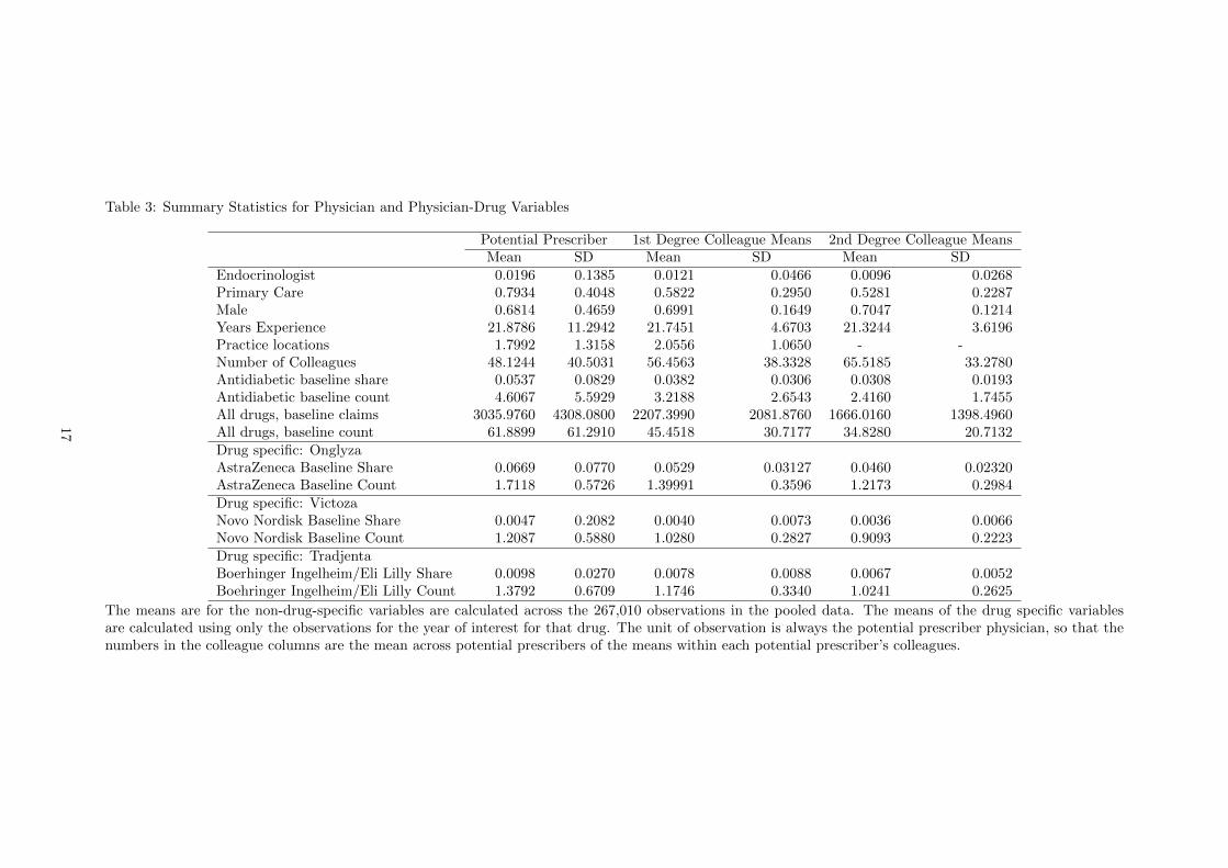
Table 3: Summary Statistics for Physician and Physician-Drug Variables

Potential Prescriber 1st Degree Colleague Means 2nd Degree Colleague MeansMean SD Mean SD Mean SD

Endocrinologist 0.0196 0.1385 0.0121 0.0466 0.0096 0.0268Primary Care 0.7934 0.4048 0.5822 0.2950 0.5281 0.2287Male 0.6814 0.4659 0.6991 0.1649 0.7047 0.1214Years Experience 21.8786 11.2942 21.7451 4.6703 21.3244 3.6196Practice locations 1.7992 1.3158 2.0556 1.0650 - -Number of Colleagues 48.1244 40.5031 56.4563 38.3328 65.5185 33.2780Antidiabetic baseline share 0.0537 0.0829 0.0382 0.0306 0.0308 0.0193Antidiabetic baseline count 4.6067 5.5929 3.2188 2.6543 2.4160 1.7455All drugs, baseline claims 3035.9760 4308.0800 2207.3990 2081.8760 1666.0160 1398.4960All drugs, baseline count 61.8899 61.2910 45.4518 30.7177 34.8280 20.7132Drug specific: OnglyzaAstraZeneca Baseline Share 0.0669 0.0770 0.0529 0.03127 0.0460 0.02320AstraZeneca Baseline Count 1.7118 0.5726 1.39991 0.3596 1.2173 0.2984Drug specific: VictozaNovo Nordisk Baseline Share 0.0047 0.2082 0.0040 0.0073 0.0036 0.0066Novo Nordisk Baseline Count 1.2087 0.5880 1.0280 0.2827 0.9093 0.2223Drug specific: TradjentaBoerhinger Ingelheim/Eli Lilly Share 0.0098 0.0270 0.0078 0.0088 0.0067 0.0052Boehringer Ingelheim/Eli Lilly Count 1.3792 0.6709 1.1746 0.3340 1.0241 0.2625

The means are for the non-drug-specific variables are calculated across the 267,010 observations in the pooled data. The means of the drug specific variablesare calculated using only the observations for the year of interest for that drug. The unit of observation is always the potential prescriber physician, so that thenumbers in the colleague columns are the mean across potential prescribers of the means within each potential prescriber’s colleagues.

17

Table 4: Adoption of Onglyza

OLS (1) OLS (2) IVEstimate SE Estimate SE Estimate SE

Constant term 0.0041 0.0037 -0.0050 0.0074 -0.0035 0.0084Indicator for Colleague Adoption 0.0325*** 0.0015 0.0313*** 0.0016 0.0398* 0.0230Endocrinologist 0.0966*** 0.0069 0.0991*** 0.0071 0.0985*** 0.0073Primary Care -0.0051** 0.0022 0.0031 0.0026 0.0026 0.0029Male 0.0107*** 0.0016 0.0098*** 0.0016 0.0097*** 0.0016Years Experience -0.0001** 0.0001 -0.0001** 0.0001 -0.0001* 0.0001Practice locations 0.0001 0.0005 0.0001 0.0007 0.00002 0.0008

Own characteristics Number of Colleagues -0.0002*** 0.00002 -0.0002*** 0.0000 -0.0002* 0.0001Same firm baseline share 0.0838*** 0.0107 0.0734*** 0.0109 0.0725*** 0.0111Same firm baseline count -0.0174*** 0.0017 -0.0165*** 0.0017 -0.0164*** 0.0018Antidiabetic baseline share -0.0467*** 0.0119 -0.0392*** 0.0119 -0.0391*** 0.0119Antidiabetic baseline count 0.0119*** 0.0003 0.0118*** 0.0003 0.0117*** 0.0004All drugs, baseline claims 1.90e-06*** 4.10e-07 2.05e-06*** 4.25e-07 2.08e-06*** 4.34e-07All drugs, baseline count 0.00003 0.00004 0.00001 0.00004 9.77e-06 0.00005Endocrinologist 0.0500** 0.0212 0.0441* 0.0266Primary Care -0.0086** 0.0038 -0.0082** 0.0039Male 0.0176*** 0.0050 0.0162** 0.0063Years Experience -0.0001 0.0002 -0.0001 0.0002Practice Locations -0.0004 0.0009 -0.0002 0.0011Number of colleagues 0.00002 0.00003 0.00008 0.00002

1st-degree colleague ave Same firm baseline share 0.1426*** 0.0320 0.1448*** 0.0325Same firm baseline count -0.0046 0.0041 -0.0045 0.0041Antidiabetic baseline share -0.1912*** 0.0420 -0.1844*** 0.0459Antidiabetic baseline count 0.0041*** 0.0010 0.0037** 0.0015All drugs, baseline claims -1.61e-06 9.92e-07 -1.36e-06 1.19e-06All drugs, baseline count -0.0001 0.0001 -0.0002 0.0001Number of Observations 87,048 87,048 86,900Adjusted R-squared 0.1271 0.1281 -First-stage F-statistic - - 71.92

The outcome variable is the adoption indicator for Onglyza. For the instrumental variables specification, the instruments are the mean over second degreecolleagues of: endocrinology indicator, primary care indicator, male indicator, same firm share, same firm distinct drug count, and number of colleagues. *indicates significance at the 10% level, ** indicates significance at the 5% level and *** indicates significance at the 1% level.

18

Table 5: Adoption of Victoza

OLS (1) OLS (2) IVEstimate SE Estimate SE Estimate SE

Constant term 0.0134*** 0.0024 0.0061 0.0054 0.0092 0.0057Indicator for Colleague Adoption 0.0215*** 0.0012 0.0198*** 0.0012 0.0888*** 0.0333Endocrinologist 0.2627*** 0.0052 0.2590*** 0.0054 0.2519*** 0.0065Primary Care -0.0092*** 0.0015 -0.0040** 0.0018 -0.0096*** 0.0033Male 0.0053*** 0.0012 0.0047*** 0.0012 0.0044*** 0.0012Years Experience -0.0003*** 0.0001 -0.0003*** 0.0001 -0.0003*** 0.0001Practice locations -0.0001 0.0004 0.0004 0.0005 0.0001 0.0006

Own characteristics Number of Colleagues -0.0001*** 0.00001 -0.0001*** 0.0000 -0.0004*** 0.0002Same firm baseline share 0.2388*** 0.0316 0.2306*** 0.0317 0.2343*** 0.0323Same firm baseline count -0.0097*** 0.0014 -0.0097*** 0.0014 -0.0086*** 0.0015Antidiabetic baseline share 0.0366*** 0.0092 0.0397*** 0.0093 0.0376*** 0.0095Antidiabetic baseline count 0.0082*** 0.0003 0.0083*** 0.0003 0.0083*** 0.0003All drugs, baseline claims 1.56e-06*** 3.02e-07 1.73e-06*** 3.14e-07 2.11e-06*** 3.67e-07All drugs, baseline count -0.0002*** 0.00003 -0.0003*** 0.00003 -0.0003*** 0.00004Endocrinologist 0.0893*** 0.0163 -0.0050 0.0484Primary Care -0.0057** 0.0028 0.0039 0.0055Male 0.0120*** 0.0038 0.0086** 0.0042Years Experience -0.0001 0.0001 -0.0001 0.0001Practice Locations -0.0013* 0.0007 0.0009 0.0012Number of colleagues 0.00003 0.00003 -0.0001* 0.00003

1st-degree colleague ave Same firm baseline share 0.1337 0.0873 -0.0345 0.1202Same firm baseline count 0.0061 0.0038 0.0081** 0.0040Antidiabetic baseline share -0.0910*** 0.0308 -0.0462 0.0380Antidiabetic baseline count -0.0007 0.0007 -0.0031** 0.0014All drugs, baseline claims -1.12e-06 -1.12e-06 1.63e-06 1.52e-06All drugs, baseline count 0.0001 0.0001 -0.0002 0.0002Number of Observations 89,309 89,203 89,203Adjusted R-squared 0.1399 0.1410 -First-stage F-statistic - - 21.64

The outcome variable is the adoption indicator for Victoza. For the instrumental variables specification, the instruments are the mean over second degreecolleagues of: endocrinology indicator, primary care indicator, male indicator, same firm share, same firm distinct drug count, and number of colleagues. *indicates significance at the 10% level, ** indicates significance at the 5% level and *** indicates significance at the 1% level.

19

Table 6: Adoption of Tradjenta

OLS (1) OLS (2) IVEstimate SE Estimate SE Estimate SE

Constant term 0.0207*** 0.0030 0.0122* 0.0066 0.0312*** 0.0080Indicator for Colleague Adoption 0.0376*** 0.0014 0.0343*** 0.0015 0.1576*** 0.0276Endocrinologist 0.2065*** 0.0064 0.2031*** 0.0066 0.1950*** 0.0070Primary Care -0.0040** 0.0019 0.0012 0.0023 -0.0069** 0.0030Male 0.0054*** 0.0015 0.0052*** 0.0015 0.0042*** 0.0016Years Experience -0.0005*** 0.0001 -0.0005*** 0.0001 -0.0005*** 0.0001Practice locations -0.0004 0.0005 -0.0015** 0.0007 -0.0040*** 0.0009

Own characteristics Number of Colleagues -0.0003*** 0.00002 -0.0002*** 0.00003 -0.0007*** 0.0001Same firm baseline share 0.0243 0.0262 0.0253 0.0263 0.0268 0.0272Same firm baseline count -0.0096*** 0.0016 -0.0095*** 0.0016 -0.0075*** 0.0017Antidiabetic baseline share 0.0039 0.0112 0.0060 0.0113 0.0010 0.0117Antidiabetic baseline count 0.0100*** 0.0003 0.0096*** 0.0003 0.0093*** 0.0004All drugs, baseline claims 4.70e-06*** 3.96e-07 4.81e-06*** 4.09e-07 5.34e-06*** 4.40e-07All drugs, baseline count -0.0003*** 0.00004 -0.0003*** 0.00004 -0.0004*** 0.00004Endocrinologist 0.0761*** 0.0200 -0.0458 0.0342Primary Care -0.0127*** 0.0035 -0.0098*** 0.0037Male 0.0104** 0.0047 -0.0118* 0.0070Years Experience 0.0006*** 0.0002 0.0005** 0.0002Practice Locations 0.0012 0.0008 0.0040*** 0.0011Number of colleagues -0.0002*** 0.0000 -0.0002*** 0.00003

1st-degree colleague ave Same firm baseline share 0.0007 0.0827 -0.0184 0.0858Same firm baseline count -0.0056 0.0044 -0.0013 0.0046Antidiabetic baseline share -0.1265*** 0.0387 -0.1004** 0.0405Antidiabetic baseline count 0.0056*** 0.0009 -0.0011 0.0018All drugs, baseline claims -1.29e-06 9.51e-07 1.45e-06 1.16e-06All drugs, baseline count -0.0002* 0.0001 -0.0004*** 0.0001Number of Observations 90,653 90,564 90,564Adjusted R-squared 0.1150 0.1166 -First-stage F-statistic - - 47.80

The outcome variable is the adoption indicator for Tradjenta. For the instrumental variables specification, the instruments are the mean over second degreecolleagues of: endocrinology indicator, primary care indicator, male indicator, same firm share, same firm distinct drug count, and number of colleagues. *indicates significance at the 10% level, ** indicates significance at the 5% level and *** indicates significance at the 1% level.

20

Table 7: Drug Adoption in Panel Data Model

FE FE/IVEstimate SE Estimate SE

Constant term -0.0036 0.0037 -0.0510*** 0.0071Indicator for Colleague Adoption 0.0257*** 0.0012 0.2134*** 0.0231

Own Characteristics Same firm baseline share 0.0612*** 0.0100 0.0636*** 0.0107Same firm baseline count -0.0059*** 0.0014 -0.0083*** 0.0015

1st-degree colleague ave Same firm baseline share -0.0476* 0.0245 -0.0656** 0.0263Same firm baseline count 0.0345*** 0.0036 0.0091* 0.0049

Fixed Effects Physician Fixed Effects Yes YesDrug Fixed Effects Yes YesNumber of Observations 267,010Number of Groups (physicians) 94,554

The outcome variable is the drug adoption indicator. For the instrumental variables specification, theinstruments are the mean over second degree colleagues of the same firm share and same firm distinctdrug count. * indicates significance at the 10% level, ** indicates significance at the 5% level and ***indicates significance at the 1% level.

21

References

[1] Baker, L. C., Bundorf, M. K., Royalty, A. B., and Levin, Z. (2014). “Physician practice competition

and prices paid by private insurers for office visits.” JAMA, 312(16), 1653-1662.

[2] Berndt, E. R., Pindyck, R. S., and Azoulay, P. (2003). “Consumption Externalities and Diffusion in

Pharmaceutical Markets: Antiulcer Drugs.” Journal of Industrial Economics, 51(2), 243-270.

[3] Bramoulle, Y., Djebbari, H., and Fortin, B. (2009). “Identification of peer effects through social

networks.” Journal of Econometrics, 150(1), 41-55.

[4] Ching, A., and Ishihara, M. (2010). “The effects of detailing on prescribing decisions under quality

uncertainty.” Quantitative Marketing and Economics, 8(2), 123-165.

[5] Chintagunta, P. K., Jiang, R., and Jin, G. Z. (2009). “Information, learning, and drug diffusion:

The case of Cox-2 inhibitors.” Quantitative Marketing and Economics, 7(4), 399-443.

[6] Claussen, J., Engelstaetter, B., and Ward, M. R. (2014). “Susceptibility and influence in social media

word-of-mouth.” ZEW-Centre for European Economic Research Discussion Paper, (14-129).

[7] Coleman, J., Katz, E., and Menzel, H. (1957). “The Diffusion of an Innovation among Physicians.”

Sociometry, 20(4), 253-270.

[8] Conley, T. G., Udry, C. R. (2010). “Learning about a new Technology: Pineapple in Ghana.” The

American Economic Review, 35-69.

[9] Crawford, G. S., and Shum, M. (2005). “Uncertainty and learning in pharmaceutical demand.”

Econometrica, 73(4), 1137-1173.

[10] Dave, Dhaval M. (2013) “Effects of Pharmaceutical Promotion: A Review and Assessment.” NBER

Working Paper w18830.

[11] De Giorgi, G., Frederiksen, A., and Pistaferri, L. (2013). “Consumption network effects.” Working

Paper.

[12] De Giorgi, G., Pellizzari, M., and Redaelli, S. (2010). “Identification of social interactions through

partially overlapping peer groups.” American Economic Journal: Applied Economics, 241-275.

[13] Dunn, A., and Shapiro, A. H. (2014). “Do physicians possess market power?.” Journal of Law and

Economics, 57(1), 159-193.

[14] Epple, D., and Romano, R. (2011). “Peer effects in education: A survey of the theory and evidence.”

Handbook of Social Economics, 1(11), 1053-1163.

[15] Karaca-Mandic, P., Town, R. J., and Wilcock, A. (2016). “The Effect of Physician and Hospital

Market Structure on Medical Technology Diffusion.” Health Services Research, in press.

22

[16] Manchanda, P., Wittink, D.R., Ching, A., Cleanthous, P., Ding, M., Dong, X.J., Leeflang, P.S.,

Misra, S., Mizik, N., Narayanan, S. and Steenburgh, T. (2005). “Understanding Firm, Physician

and Consumer Choice Behavior in the Pharmaceutical Industry.” Marketing Letters, 16(3-4),

293-308.

[17] Manski, C. F. (1993). “Identification of endogenous social effects: The reflection problem.” The

Review of Economic Studies, 60(3), 531-542.

[18] Moffitt, R. A. (2001). “Policy interventions, low-level equilibria, and social interactions.” Social

Dynamics, 4(45-82), 6-17.

[19] Nair, H. S., Manchanda, P., and Bhatia, T. (2010). “Asymmetric social interactions in physician

prescription behavior: The role of opinion leaders.” Journal of Marketing Research, 47(5), 883-

895.

[20] Saxell, T. (2014). “Private experience and observational learning in pharmaceutical demand.” Work-

ing paper.

[21] Town, R., Feldman, R., and Kralewski, J. (2011). “Market power and contract form: Evidence from

physician group practices.” International Journal of Health Care Finance and Economics, 11(2),

115-132.

[22] Welch, W. P., Cuellar, A. E., Stearns, S. C., and Bindman, A. B. (2013). “Proportion of physicians

in large group practices continued to grow in 2009-11.” Health Affairs, 32(9), 1659-1666.

23