physical wave propagation modeling for real-time synthesis of natural sounds
TRANSCRIPT

PHYSICAL WAVE PROPAGATION MODELING
FOR REAL-TIME SYNTHESIS OFNATURAL
SOUNDS
GEORGESSL
A D ISSERTATION
PRESENTED TO THEFACULTY
OF PRINCETON UNIVERSITY
IN CANDIDACY FOR THE DEGREE
OF DOCTOR OFPHILOSOPHY
RECOMMENDED FORACCEPTANCE
BY THE DEPARTMENT OF
COMPUTERSCIENCE
NOVEMBER 2002

c© Copyright by Georg Essl, 2002. All rights reserved.

iii
Abstract
This thesis proposes banded waveguide synthesis as an approach to real-time sound
synthesis based on the underlying physics. So far three main approaches have been
widely used: digital waveguide synthesis, modal synthesis and finite element methods.
Digital waveguide synthesis is efficient and realistic and captures the complete dynamics
of the underlying physics but is restricted to instruments that are well-described by the
one-dimensional string equation. Modal synthesis is efficient and realistic yet abandons
complete dynamical description and hence cannot used for certain types of performance
interactions like bowing. Finite element methods are realistic and capture the behavior of
the constituent physical equations but on current commodity hardware does not perform
in real-time.
Banded waveguides offer efficient simulations for cases for which modal synthesis
is appropriate but traditional digital waveguide synthesis is not applicable. The key
realization is that the dynamic behavior of traveling waves, which is being used in waveg-
uide synthesis, can be applied to individual modes and that the efficient computational
structure can be utilized to achieve an approximate dynamical description in the neigh-
borhood of modes. Secondly this realization is connected to related work on the theory
of asymptotics and periodic orbits and hence shown to apply to higher dimensions also.
This theoretical approach is studied in applications to bowed bar percussion instru-
ments, complex stroke patterns on Indian Tabla drums as well as rubbed wine glasses
and Tibetan singing bowls. None of these instruments and performance types has been
synthesized efficiently before. The simulations are compared to experiments.
iv
Acknowledgments
Since this was written and needs must be —
My whole heart rises up to bless
Your name in pride and thankfulness! – Robert Browning1
There is much to be thankful for and I will definitely not do everyone and everything
justice that helped me work on and complete this thesis.
Piles of gratitude are due to my advisor Prof. Perry R. Cook. I had not anticipated
how good a match Perry would be for me. Not only is he at the very frontier of physical
modeling of sound, but also did he provide the interactions, freedoms, supports and
atmosphere I needed, academically and beyond. He handled my doubts and uncertainties
with grace that is rare to be found.
Also Prof. Ken Steiglitz was a great man to be around (and he is a giant for his
size). I had uncountable enjoyable conversations, whether it was scientific or humoristic,
political or casual. A source of ideas, experience and knowledge and a role-model for
open-mindedness, curiosity and versatility. Profs. Tom Funkhouser — who also dug
through all these pages as a reader — and Adam Finkelstein sat through many a talks
of mine gave me advice on publishing or on questions concerning graphics. Also Prof.
Paul Lansky for the kindness of being on my committee and hence agreeing to put up
with tons of “engineer’s speak”. All of them were great sources of feedback during the
formation process of this thesis.
Lots of thanks to George Tzanetakis, as collaborator, lab fellow, dog owner and more.
I greatly enjoyed the collaboration with Prof. James. F. O’Brien and a visit at
Berkeley. Professors J. P. Singh, Kai Li, Jonathan Cohen, Joan Girgus and John Hop-
1“The Last Ride Together,” lines 5-7, (1855) in Arthur Quiller-Couch, ed. “The Oxford Book of EnglishVerse” (1919) available online atwww.bartleby.com/101/727.html also [147, p. 150, q. 19].

v
field were a great resource during me exploration for the right direction of research at
Princeton. Needless to say I had countless great exchanges, help, support and fun with
many people in the department including Melissa, Ginny, Trish, Mitra, Tina, also Profs.
Bernhard “Santana” Chazelle (thanks for the jam sessions), Szymon Rusinkiewicz, Ben
Shedd, Brian Kernighan, Mona Singh, Andrew “Expresso” Appel (thanks for keeping
the caffeine coming!), David August, Randy Wang and Doug Clark. Many thanks to
Department Chair David Dobkins for lots of guidance.
Best thanks also to Gary Scarvone for insightful feedback on banded waveguide
implementations in STK, in particular with regards to bandwidth questions. To Professor
Julius Smith for the kind permission to use the Friedlander-Keller diagram (see Figure
2.8) from him book-in-progress. Ed Gaida for the kind permission to use his beauti-
ful photograph of Franklin’s glass harmonica (see Figure 4.23), James F. O’Brien for
rendered bowl mode shapes (see Figure 4.26) and Ajay Kapur for his tabla picture (see
Figure 4.18).
Davide Rocchesso, Ingolf Bork, Antoine Chaigne, Bob Schumacher, Chris Chafe,
Anindya Ghoshal and Rolf Runborg kindly provided reprints, advice and feedback of
various sorts.
Also thanks to Jim Johnston and Schuyler Quakenbush of AT&T Research.
Tons of thanks to Lujo Bauer, the first friend I made in Princeton and the best I had
throughout the years.
Also best thanks to all my office mates, Ben Dressner, Wagner Correa, late Cheng
Liao, Eun-Young Lee, Dongming Jiang, Yilei Shao, Bo Brinkman, Chris Richards, Sumeet
Sobti, Tony Wirth, Fengzhou Zheng and John Hainsworth for providing both a friendly
environment and necessary diversions. And all the people I enjoyed outside my office,
including but by no means limited to Iannis “Rager” Tourlakis, Amal Ahmed, Jie Chen,

vi
Mattias Jacob, Allison Klein, Ketan Dalal, Neophytos Michael, Patrick Min, Emil Praun,
Ricki Smith, Yefim Shuf, John Forsyth, Kedar Swadi, Gary Wang, Dan Wang, Brent
Waters, Matt Webb, Jiannan Chen, Wenjia Fang, Dirk Balfanz, Rudro Samanta, Tammo
Spalink, Lena Petrovic, Limin Wang, Limin Jia, Jessica Wang, Lisa Worthington and
Kevin Wayne.
Undergrads I worked with Ajay Kapur, Neal Shah, Anoop Gupta, Gakushi Nakamura,
Fei-Fei Li, Cory Elder and Hagos Mehreteab.
And to all the friends in all the other colleagues in the departments and all the in-
teresting people I got to meet. Kai Chen for his friendship and hour-long discussions
of ethics. Sharon Bingham, Troy Smith, Matt Hindman, Andy Burlingame, Jo Hertel,
Steven Miller, Kyoko Sato, Johannes Chudoba, Debbie Abrams, Yesim Tozan, Mikalis
Dafermos, Matt Devos, Adrian Banner, Konstantinos Drakakis, Tessy Papavasiliou, Yan-
nis Papadoyannakis, Lyndon Dominique, Ilana Moreno-Shields, Emily Doolittle, Mary
Wright, Azul Wright, Colby Leider, Tae-Hong Park, Laurie Hollander, Dan Trueman,
Monica Mugan, Jennifer Burkowski, Kim Weaver, Jeff, Vera Koffman, Tim Hall, Tre
Green, Herdes Teich, Mike Buchanan, Sarah Thomas, Cliona Golden, Steve Tibbets,
Traci, Ade, Sinda, Natasha, Joe, the FireHazards, especially Chinook, Anina, Chuck,
Greg, Maria, Liz, Betsy, Christina, Katherine, and Sarah Rod plus all the newbies Laure,
“Ardvark”, Tudor, Chinny, Sarahs (both), Holly, Janine and Paris. Family and friends
back home (Peter, Andy) or scattered around the globe (Jorg, Robert) are last but never
least. Love you guys, thanks for all.
Of course I’m grateful for financial support throughout the years. My first two years
of work has been supported by a post-graduate stipend of the Austrian Federal Ministry
of Science and Education. In later years I enjoyed industrial support through Intel, Arial

vii
and Microsoft and academic support through NSF Grant Number 9984087 and the State
of New Jersey Commission on Science and Technology Grant Number 01-2042-007-22.

viii
Dedicated to my parents.
To my mom who gave me the love of music,
and my dad who gave me the love of science.

Contents
Abstract . . . . . . . . . . . . . . . . . . . . . . . . . . . . . . . . . . . . . . iii
1 Introduction 1
1.1 The Thesis Stated . . . . . . . . . . . . . . . . . . . . . . . . . . . . . . 1
1.2 Contributions of this Thesis . . . . . . . . . . . . . . . . . . . . . . . . . 2
1.2.1 Publications and their Place in this Thesis . . . . . . . . . . . . . 3
1.3 Thesis Outline . . . . . . . . . . . . . . . . . . . . . . . . . . . . . . . . 4
2 Background, Previous Art and Related Literature 5
2.1 Sound Synthesis Methods . . . . . . . . . . . . . . . . . . . . . . . . . . 8
2.1.1 Waveguide Synthesis . . . . . . . . . . . . . . . . . . . . . . . . 10
2.1.2 Finite Element Methods . . . . . . . . . . . . . . . . . . . . . . 14
2.1.3 Modal Synthesis . . . . . . . . . . . . . . . . . . . . . . . . . . 17
2.2 Excitations . . . . . . . . . . . . . . . . . . . . . . . . . . . . . . . . . 19
2.2.1 Linear or Impulsive Excitation . . . . . . . . . . . . . . . . . . . 19
2.2.2 Nonlinear or Friction Excitation: Stick-Slip . . . . . . . . . . . . 20
3 Theory of Propagation Modeling 23
3.1 Overview and Motivation of Propagation Modeling for Sound Synthesis . 24
3.1.1 Local Displacement to Moving Disturbance . . . . . . . . . . . . 24
ix

CONTENTS x
3.1.2 Propagation of Sound in Air . . . . . . . . . . . . . . . . . . . . 25
3.1.3 Guided Waves . . . . . . . . . . . . . . . . . . . . . . . . . . . 26
3.1.4 Limits and Alternatives to Propagation Modeling so Far . . . . . 26
3.2 A Sketch: Generalizing the Propagation Idea . . . . . . . . . . . . . . . 27
3.3 Description of Abstract Banded Waveguides . . . . . . . . . . . . . . . . 31
3.3.1 Notation . . . . . . . . . . . . . . . . . . . . . . . . . . . . . . 33
3.4 Banded Digital Waveguides as Filters . . . . . . . . . . . . . . . . . . . 34
3.4.1 Domain Decomposition Filtering . . . . . . . . . . . . . . . . . 34
3.4.2 Constant-Speed Wave Propagation Filter: Delay line . . . . . . . 35
3.4.3 The Perturbation Filter . . . . . . . . . . . . . . . . . . . . . . . 36
3.4.4 Domain Reconstruction Filtering . . . . . . . . . . . . . . . . . . 36
3.5 Banded Digital Waveguides as Phase-Corrected Modal Synthesis . . . . . 37
3.6 Banded Digital Waveguides as Generalized Digital Waveguides . . . . . . 38
3.7 Banded Digital Waveguides as Multi-scale Numerical Method . . . . . . 39
3.8 Banded Digital Waveguides as Discrete Asymptotics Simulation . . . . . 41
3.8.1 Previous Work: Traveling Wave Solutions . . . . . . . . . . . . . 41
3.8.2 Previous Work: Numerical Traveling Waves . . . . . . . . . . . . 43
3.8.3 Discrete Asymptotic Simulation . . . . . . . . . . . . . . . . . . 45
3.9 Banded Digital Waveguides in Higher Dimensions . . . . . . . . . . . . 47
3.9.1 Previous Work: Single-band Multi-path or Multi-dimensional Mod-
els . . . . . . . . . . . . . . . . . . . . . . . . . . . . . . . . . . 48
3.9.2 Topology of Resonant Paths . . . . . . . . . . . . . . . . . . . . 49
3.10 Theory to Application: Use of Banded Waveguides . . . . . . . . . . . . 54
3.10.1 Physical Simulation . . . . . . . . . . . . . . . . . . . . . . . . 54
3.10.2 Application as Non-physical Entities . . . . . . . . . . . . . . . . 56

CONTENTS xi
3.11 Performance and Critical Sampling . . . . . . . . . . . . . . . . . . . . . 56
3.12 Interaction Models . . . . . . . . . . . . . . . . . . . . . . . . . . . . . 57
3.13 Conclusions . . . . . . . . . . . . . . . . . . . . . . . . . . . . . . . . . 58
4 Applications of the Banded Digital Waveguides 59
4.1 1-D Case: Rigid Bars . . . . . . . . . . . . . . . . . . . . . . . . . . . . 60
4.1.1 Simulations . . . . . . . . . . . . . . . . . . . . . . . . . . . . . 61
4.1.2 Experimental Measurements . . . . . . . . . . . . . . . . . . . . 69
4.2 2-D Case: Indian Tabla Drums . . . . . . . . . . . . . . . . . . . . . . . 87
4.2.1 Periodic Orbit on Circular Domain . . . . . . . . . . . . . . . . . 91
4.3 3-D Case I: Wine Glasses and Glass Harmonicas . . . . . . . . . . . . . 94
4.4 3-D Case II: Tibetan Singing Bowl . . . . . . . . . . . . . . . . . . . . . 97
4.4.1 Beating Banded Waveguides . . . . . . . . . . . . . . . . . . . . 99
5 Comparison with Alternative Methods 103
5.1 Modal Synthesis . . . . . . . . . . . . . . . . . . . . . . . . . . . . . . . 103
5.2 Waveguide Synthesis . . . . . . . . . . . . . . . . . . . . . . . . . . . . 104
5.3 All-pass Chains and Frequency Warping . . . . . . . . . . . . . . . . . . 105
5.4 Modal Decomposition & Green’s Function . . . . . . . . . . . . . . . . . 108
5.5 Finite Element Methods . . . . . . . . . . . . . . . . . . . . . . . . . . . 108
6 Geometric Simulation Using Finite Elements 111
6.1 Sound Modeling . . . . . . . . . . . . . . . . . . . . . . . . . . . . . . . 112
6.1.1 Motions of Solid Objects . . . . . . . . . . . . . . . . . . . . . . 112
6.1.2 Surface Vibrations . . . . . . . . . . . . . . . . . . . . . . . . . 114
6.1.3 Wave Radiation and Propagation . . . . . . . . . . . . . . . . . . 115

CONTENTS xii
6.2 Results . . . . . . . . . . . . . . . . . . . . . . . . . . . . . . . . . . . . 116
7 Conclusions, Future Directions and Applications 122
7.1 Conclusions . . . . . . . . . . . . . . . . . . . . . . . . . . . . . . . . . 123
7.2 Separation of Wavetrains and Geometry . . . . . . . . . . . . . . . . . . 123
7.3 The Link Between Lumped Modal Synthesis and Digital Waveguide Syn-
thesis . . . . . . . . . . . . . . . . . . . . . . . . . . . . . . . . . . . . 125
7.4 The Link Between Geometry and Modes . . . . . . . . . . . . . . . . . . 126
7.4.1 Geometry, Modes and Efficiency . . . . . . . . . . . . . . . . . . 126
7.5 Summary . . . . . . . . . . . . . . . . . . . . . . . . . . . . . . . . . . 127
7.6 Future Work . . . . . . . . . . . . . . . . . . . . . . . . . . . . . . . . . 128
7.6.1 Perceptual Measures for Synthesis Methods . . . . . . . . . . . . 128
7.6.2 Waveguide Preconditioning for Matrix Methods . . . . . . . . . . 129
7.6.3 Multirate Banded Waveguides, Perturbations and Extensions in
the Banded Case . . . . . . . . . . . . . . . . . . . . . . . . . . 130
A Glossary for Asymptotics Terms 131
B Implementation 135
Index of Authors 139
Bibliography 145

List of Figures
1.1 The object of the thesis. . . . . . . . . . . . . . . . . . . . . . . . . . . . 2
2.1 Reflection of a traveling wave on a boundary. . . . . . . . . . . . . . . . 11
2.2 Waveguide synthesis of ideal lossless string . . . . . . . . . . . . . . . . 12
2.3 The Karplus-Strong algorithm as waveguide synthesis. . . . . . . . . . . 13
2.4 A finite difference simulation of a tuned bar (using the method of Chaigne
and Doutaut [35]) . . . . . . . . . . . . . . . . . . . . . . . . . . . . . . 15
2.5 Tetrahedral mesh for anF]3 vibraphone bar. In (a), only the external
faces of the tetrahedra are drawn; in (b) the internal structure is shown.
Mesh resolution is approximately1cm. . . . . . . . . . . . . . . . . . . . 15
2.6 Computational molecules of (a) second order and (b) fourth order dis-
cretizations leading to banded entry in the model matrix of a finite ele-
ment solver. . . . . . . . . . . . . . . . . . . . . . . . . . . . . . . . . . 16
2.7 A mass-spring damper system and connected digital filter simulation . . . 17
2.8 Friedlander-Keller friction diagram (from [188]). . . . . . . . . . . . . . 21
3.1 Input, propagation system, output. . . . . . . . . . . . . . . . . . . . . . 25
3.2 A single banded wave-path.BP is a band-pass filter. . . . . . . . . . . . . 29
3.3 A simple banded waveguide system. . . . . . . . . . . . . . . . . . . . . 30
xiii

LIST OF FIGURES xiv
3.4 A banded waveguide system including explicit modeling of the reflection. 31
3.5 Abstract depiction of the cyclic property of domains and their decompo-
sitions . . . . . . . . . . . . . . . . . . . . . . . . . . . . . . . . . . . . 33
3.6 (a) Constant time representation and (b) constant space representation of
a banded wave-path. . . . . . . . . . . . . . . . . . . . . . . . . . . . . 40
3.7 A digital waveguide filter. . . . . . . . . . . . . . . . . . . . . . . . . . . 44
3.8 Reflection of a ray at the boundary . . . . . . . . . . . . . . . . . . . . . 50
3.9 Resonant torus of EBK quantization of two-dimensional closed paths. . . 51
3.10 Relationship of geometry and dynamics to modes. . . . . . . . . . . . . . 54
4.1 Discretization of the phase delay in a banded waveguide simulation. . . . 63
4.2 One banded waveguide (top) and its spectrum. . . . . . . . . . . . . . . . 64
4.3 Friction characteristic used in the banded waveguide simulation. For a
relative velocity around zero, the bow exerts a nearly constant strong
static friction on the bow whereas when exceeding the relative break-
away velocity, the characteristics drops quickly to low dynamic friction. . 67
4.4 Amplitude as a function of input force and velocity in a bowed bar simu-
lation using the banded waveguide method. . . . . . . . . . . . . . . . . 69
4.5 Onset time as a function of input force in a bowed bar simulation using
the banded waveguide method. . . . . . . . . . . . . . . . . . . . . . . . 70
4.6 Sketch of shape and dimensions of a bar. . . . . . . . . . . . . . . . . . . 72
4.7 Experimental setup for hand bowing measurements of bars. . . . . . . . . 74
4.8 Time-domain amplitude envelope of hand strokes with increasing veloc-
ity and force held approximately constant. . . . . . . . . . . . . . . . . . 76
LIST OF FIGURES xv
4.9 Time-domain amplitude envelope of hand strokes with increasing force
and velocity held approximately constant. . . . . . . . . . . . . . . . . . 77
4.10 Experimental setup for bowing machine measurements of bars. . . . . . . 78
4.11 Bowing machine measurement series 1: Measured input parameters: Force
and velocity. . . . . . . . . . . . . . . . . . . . . . . . . . . . . . . . . . 79
4.12 Bowing machine measurement series 2: Measured input parameters: Force
and velocity. . . . . . . . . . . . . . . . . . . . . . . . . . . . . . . . . . 80
4.13 Bowing machine measurement series 1: Recorded radiation energy as a
function of bowing velocity. . . . . . . . . . . . . . . . . . . . . . . . . 82
4.14 Bowing machine measurement series 2: Recorded radiation energy as a
function of bowing force. . . . . . . . . . . . . . . . . . . . . . . . . . . 83
4.15 Bowing machine measurement series 1: Spectral centroid as a function
of bowing force. Only measurement point with a clear steady-state oscil-
lation are shown. . . . . . . . . . . . . . . . . . . . . . . . . . . . . . . 84
4.16 Bowing machine measurement series 2: Onset time as a function of
bowing force. . . . . . . . . . . . . . . . . . . . . . . . . . . . . . . . . 85
4.17 Bowing machine measurement series 2: Onset time as a function of
bowing velocity. . . . . . . . . . . . . . . . . . . . . . . . . . . . . . . . 86
4.18 Indian Tabla drums played by Ajay Kapur. . . . . . . . . . . . . . . . . . 87
4.19 The nine nodal patterns of the Tabla tuned to harmonic modes (after
Rossing [173]). . . . . . . . . . . . . . . . . . . . . . . . . . . . . . . . 89
4.20 Spectrogram showing the upward bending of a modulatedGastroke. The
fundamental bends from 136 to 162 Hz (measured) and 134 to 171 Hz
(simulated). . . . . . . . . . . . . . . . . . . . . . . . . . . . . . . . . . 90

LIST OF FIGURES xvi
4.21 Radial and angular variables on a circular domain and their connected
turning properties. . . . . . . . . . . . . . . . . . . . . . . . . . . . . . . 91
4.22 Keller-Rubinow path construction on the circular domain (compare [104,
Fig. 3 and 5]). (a) Closed path touching the interior caustic. (b) Radius
of the caustic circle. (c) Path containing rays traveling from caustic to
boundary and back. . . . . . . . . . . . . . . . . . . . . . . . . . . . . . 93
4.23 Benjamin Franklin’s glass harmonica, which he called “armonica”, as
seen in the Franklin Institute Science Museum in Philadelphia. . . . . . . 95
4.24 The wavetrain closure on the rim of a wine glass and corresponding
flexural waves as seen from the top (after Rossing [173]). . . . . . . . . . 96
4.25 Mesh of simulated bowl. . . . . . . . . . . . . . . . . . . . . . . . . . . 98
4.26 Simulated mode shapes of the bowl. . . . . . . . . . . . . . . . . . . . . 98
4.27 Path of circular mode on bowl (used with permission from (Cook 2002).) 99
4.28 Spectra of different excitations (used with permission from (Cook 2002).) 100
4.29 Beating upper partials in spectrogram of a recorded Tibetan bowl. . . . . 101
4.30 Left: Evolution of an isolated simulation of a beating mode pair. Right:
Initial transient and the first beating period. . . . . . . . . . . . . . . . . 102
5.1 All-pass-chain or warped frequency waveguide. . . . . . . . . . . . . . . 105
5.2 All-pass filter design for a given delay characteristic (following Lang [116]).106
5.3 Labeling of delay-line cells for matrix notation. . . . . . . . . . . . . . . 109
6.1 The top image shows a multi-exposure image from an animation of a
metal bowl falling onto a hard surface. The lower image shows a spec-
trogram of the resulting audio for the first five impacts. . . . . . . . . . . 117
LIST OF FIGURES xvii
6.2 The top image plots a comparison between the spectra of a real vibra-
phone bar (Measured), and simulated results for a low-resolution (Sim-
ulated 1) and high-resolution mesh (Simulated 2). The vertical lines
located at 1, 4, and 10 show the tuning ratios reported in [70]. . . . . . . . 119
6.3 These figures show a round weight being dropped onto two different
surfaces. The surface shown in (a) is rigid while the one shown in (b)
is more compliant. . . . . . . . . . . . . . . . . . . . . . . . . . . . . . 120
6.4 A slightly bowed sheet being bent back and forth. . . . . . . . . . . . . . 120
7.1 Left: Closed paths with one reflection at each side. Right: Closed paths
with two reflection at the top and bottom and one at the sides. . . . . . . . 124
7.2 Comparison of modal synthesis, waveguides, banded waveguides and
finite element methods. . . . . . . . . . . . . . . . . . . . . . . . . . . . 128
B.1 STK graphical user interface for bars and bowls using banded waveguides. 138

Chapter 1
Introduction
There are two things which I am confident I can do very well: One is an
introduction to any literary work, stating what it is to contain, and how it should
be executed in the most perfect manner; [..]1 – Samuel Johnson2
Let me introduce to you three of my friends: the red herring called insight, the
blue trout called hindsight, and the translucent amoeba called blindsight.
1.1 The Thesis Stated
The core of the thesis is to propose the usefulness of a certain algorithm, a certain filter
structure or a certain numerical method for the real-time synthesis of sounds on the
computer. This method is depicted using a block-diagram style typical for digital filters
in Figure 1.1
1Quote continued in the concluding chapter.2James Boswell, “Life of Samuel Johnson,” (1755) available athttp://newark.rutgers.edu/
˜jlynch/Texts/BLJ/blj55.html or according to [147, p. 371, q. 17] in vol. 1, p. 292 (1755)
1

CHAPTER 1. INTRODUCTION 2
Figure 1.1: The object of the thesis.
Throughout this thesis, I will discuss properties of this structure, various forms of
conceptual interpretation and connection to physically systems as well as the relation of
this structure to prior work and knowledge. I will argue that this structure is a gener-
alization of prior methods and by this generalization allows for an extended domain of
application. I will also argue that this structure is useful for thinking about notions of
efficiency and stability for numerical simulation. Finally I’ll compare the usefulness of
the method in application and with respect to alternative methods.
The statement of my thesis is that the method, which I like to call “banded digital
waveguides,” is a significant advance in the field of physical sound simulation, by offering
a number of theoretical and practical contributions.
1.2 Contributions of this Thesis
In thesis, I propose a physical modeling method for musical instruments and other sound-
ing objects. The method itself is a generalization of previous methods and broadens their
CHAPTER 1. INTRODUCTION 3
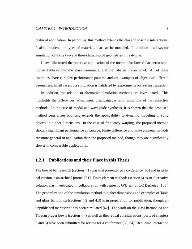
realm of application. In particular, this method extends the class of possible interactions.
It also broadens the types of materials that can be modeled. In addition it allows for
simulation of some two and three-dimensional geometries in real-time.
I have illustrated the practical application of the method for bowed bar percussion,
Indian Tabla drums, the glass harmonica, and the Tibetan prayer bowl. All of these
examples share complex performance patterns and are examples of objects of different
geometries. In all cases, the simulation is validated by experiments on real instruments.
In addition, the relation to alternative simulation methods are investigated. This
highlights the differences, advantages, disadvantages, and limitations of the respective
methods. In the case of modal and waveguide synthesis, it is shown that the proposed
method generalizes both and extends the applicability to dynamic modeling of solid
objects in higher dimensions. In the case of frequency warping, the proposed method
shows a significant performance advantage. Finite difference and finite element methods
are more general in application than the proposed method, though they are significantly
slower in comparable applications.
1.2.1 Publications and their Place in this Thesis
The bowed bar research (section 4.1) was first presented at a conference [60] and in its fi-
nal version in an archival journal [61]. Finite element methods (section 6) as an alternative
solution was investigated in collaboration with James F. O’Brien of UC Berkeley [135].
The generalization of the simulation method to higher dimensions and examples of Tabla
and glass harmonica (sections 4.2 and 4.3) is in preparation for publication, though an
unpublished manuscript has been circulated [62]. The work on the glass harmonica and
Tibetan prayer bowls (section 4.4) as well as theoretical considerations (parts of chapters
3 and 5) have been submitted for review for a conference [63, 64]. Real-time interaction
CHAPTER 1. INTRODUCTION 4
work with Ajay Kapur, Philip Davidson and Perry Cook for the Tabla drums [98] will not
be discussed here beyond the Tabla simulation.
1.3 Thesis Outline
I will first discuss the background, prior art and related literature chapter 2. Then the
theory of propagation modeling using banded waveguides will be discussed in chapter
3. Then, in chapter 4, four examples will be discussed: bar percussion instruments (sec-
tion 4.1), Indian Tabla drums (section 4.2), glass harmonicas (section 4.3), and Tibetan
singing bowls (section 4.4) with relevant experimental work. Then the simulation method
is compared with alternative methods in chapter 5 and the case of finite element methods
is described and discussed in detail in chapter 6. Finally possible future directions and
applications of the method are proposed in chapter 7.

Chapter 2
Background, Previous Art and Related
Literature
Only the more rugged mortals should attempt to keep up with current litera-
ture. – George Ade1
The combined collections total more than six million printed works, five million
manuscripts and two million nonprint items, and increase at the rate of about
10,000 volumes a month. – History of the Princeton University Library
Online2
Six months in the lab can save you a day in the library. – old reference
librarian proverb (according to Sally Jo Cunningham3) or by Albert
Migliori (according to Julian D. Maynard 4)
Information come and stay, sink in and if you don’t — go away.
1As attributed athttp://www.geocities.com/˜spanoudi/topic-I5.html2http://libweb.princeton.edu/about/history.php as retrieved on April 14, 2002.3http://www.cs.waikato.ac.nz/GradConf/talks/sallyjo/4Julian D. Maynard, “Resonant Ultrasound Spectroscopy,” Physics Today 48(1) 26-31, January 1996.
5
CHAPTER 2. BACKGROUND, PREVIOUS ART AND RELATED LITERATURE6
This work is interdisciplinary in nature. The background of this work is not solely
placed in firmly established fields within Computer Science, but rather draws on a wide
range of different disciplines, knowledge and ideas. Traditionally work along these lines
has been connected with an emerging discipline called “Computer Music” [202]. More
specifically within the sound synthesis community, this line of work falls into the category
of “physical modeling” [165, chapter 7].
The work to be presented draws from a wide range of different fields. Yet I first
want to present only the background and prior art as understood in the Computer Music
community and I would like to introduce relevant texts that are not commonly known
in the community as part of the theoretical discussion or, if applicable, in other sections
throughout this thesis. The purpose of this approach is mostly to motivate the relevance
of these works with the development of the ideas, so it can be appreciated by the commu-
nity5.
Wave phenomena are so ubiquitous that a review of knowledge pertaining to this
phenomena can be a daunting and overwhelming task and in the end it seems to me that
claims to completeness would imply proof of insanity. Still, I made an attempt to be as
broad as I possibly could be in finding material and the search for literature was confined
mostly by basic ideas presented in this thesis. Literature deemed worthy of investigation
have some connection to a number of questions:
• Who has studied wave propagation analytically and numerically and how?
• What is known about stick-slip interactions and perceptible noise generated from
it?5This is also connected with problems of presentation of interdisciplinary work, as for example noted
by Margrit Eichler [59, p. 59] of translation, language and reception. I hope of a benefit in reception ifunfamiliar literature is presented along familiar lines of arguments rather than in isolation.

CHAPTER 2. BACKGROUND, PREVIOUS ART AND RELATED LITERATURE7
• What is known about certain sounding objects, like bars, membranes, tuned bars,
tuned membranes, Tabla drums and wine glasses?
• What is known about measurement, parameter estimation of responses of the above
objects?
Also before the background search took on its full depth I knew already that in my
immediate community, people who study physical modeling of musical instruments —
a fairly small community of mostly electrical engineers, acousticians, musicians and
computer scientists — the ideas proposed in this thesis were novel. There was hence
also the question:
• Which of these ideas are known in what form outside my core community?
And finally the literature search is also a foundation of the research presented in this
thesis:
• How can literature answer questions that arise in my way of framing and investi-
gating the problem?
Investigating these last two questions leads to an assimulation of various strands of
research that are apparently (sometimes only partly) unaware of each other. For example,
the mode-ray duality is known in as diverse fields as structural engineering, seismology,
electromagnetism, theoretical physics, and applied and pure mathematics. All these fields
have, however only a partial overlapping in awareness of the connection of their work and
progression of insight in other fields. While traveling wave methods are widely used in
structural engineering [126] there seems to be little awareness of the correspondence of
their approach to asymptotic theory [139] or periodic orbits in chaos theory [48]. Even

CHAPTER 2. BACKGROUND, PREVIOUS ART AND RELATED LITERATURE8
within mathematical physics the interaction between U.S. [103], Western Europe [58],
and Russia [110] is evidently not always present (see for example remarks in [58]).
This contributes to the fact that very similar concepts in literature have very different
nomenclatures and attributions (for example, an asymptotic traveling wave Ansatz can
go by any of the following names or acronyms: LG, WKB, JWKB, EBK, periodic orbits,
traveling wave method, wave method, ray method, ray tracing method, billiard, phase
integral method, asymptotic method.) A brief glossary trying to unravel some of this
confusion can be found in Appendix A6. One contribution of this thesis is a shy attempt
to unearth these connections and find a synthesis that is approachable by the researcher
in physical modeling for sound synthesis.
All these questions will be addressed throughout the thesis. Next I would like to
review the prior art of sound synthesis as a precursor to this work.
2.1 Sound Synthesis Methods
Sound synthesis methods can be classified into various groups. The previously used
methods with direct relation to this work are generally classified asphysical modeling
synthesis[165]7. Though Roads [165] classifies many separate categories of methods
within the field, many are conceptually very closely related. For instance McIntyre,
Schumacher, and Woodhouse synthesis [122], Karplus-Strong synthesis [100, 94, 99,
195] and Waveguide synthesis [185, 187, 188] are very closely related. In the case of
Karplus-Strong and Waveguide synthesis, the difference can be seen as mere physical
interpretation of the structure.
6The confusion that is part of the process of unifying various lines of research is nicely described byDaubechies in the case of the evolution of wavelets [51].
7A related taxonomy can also be found in [198].

CHAPTER 2. BACKGROUND, PREVIOUS ART AND RELATED LITERATURE9
McIntyre, Schumacher, and Woodhouse realized that separation of non-linear ex-
citation and linear resonant instrument response with a persistence on a time-domain
view allows for quite efficient and qualitatively good simulation that captures the rich
behavior of the overall dynamics very well. The work of Karplus and Strong then
highlighted that, in fact, the traveling wave that gives rise to the resonant behavior of
strings under tension and air-filled pipes can be very efficiently modeled using delay-
lines. This efficient implementation of a delay line uses a circular buffer [55, p. 227][194,
p. 258-260], something that had been realized by Schroeder and others while studying
synthetic reverberation and room-acoustic simulation [105, 75, 76, 12, 175, 90, 28].
In the remainder of the thesis I will refer to all of these categories simply aswaveguide
synthesis8.
Another line of physical modeling are methods which are concerned with direct
discrete simulation of the local dynamics responsible for sound generation. These in-
clude methods using finite differencing [174, 33, 20, 113, 35, 146], mass-spring-damper
networks [30, 71, 31], finite element methods [27, 21] and transmission-line methods for
solving differential equations [214, 18] (which includes highly scattering digital waveg-
uide simulations and digital waveguide meshes)9. Again, all these methods are in close
relationship to each other. For instance there is a direct correspondence between finite
differencing and scattering networks [18]. Though not necessarily known in the Com-
puter Music community, the matrices arising in solid mechanics finite element methods
have a direct mass-spring-damper interpretation [222] and finite elements can be seen as
generalization of finite difference methods [222, 5, 201].
8Julius Smith often uses the termwaveguide digital synthesisto indicate that this is a digital synthesismethod, throughout this thesis all methods are digital in the sense that are all numerical discretization ondigital computers.
9This is an important note to make. Digital waveguide meshes are, for the purpose of these thesis, notclassified with waveguide simulations but rather with finite element methods.

CHAPTER 2. BACKGROUND, PREVIOUS ART AND RELATED LITERATURE10
For the purpose of this thesis I will refer to all of these methods as instances offinite
element methods.
The final class of physical synthesis methods models the spectral response of the
physical system. This can be achieved through additive sinusoidal modeling [182, 210],
resonant filter modeling [219, 42], model decomposition modeling [1].
These methods will be referred to asmodal synthesis methodsthroughout this thesis10.
Other methods of sound synthesis, as found in [165, 55, 198], are not reviewed as
they are not relevant to this thesis. They are either not physically informed or stochastic
in nature.
2.1.1 Waveguide Synthesis
There are many references which comprehensively review waveguide modeling at it
current state [188, 45, 187, 99, 8]. Here I will only mention the key ideas and ideas
in previous work that are relevant to this thesis.
The derivation of the basic idea of waveguide synthesis is usually presented starting
with the ideal wave-equation which describes the perfectly elastic string under tension
and oscillations in an air-tube or related wave-guiding structure for small displacements
[132, 194, 188]:
∂2y∂t2 = c2∂2y
∂x2 (2.1)
10Note that modal means different things to different communities. The wordmodalwas chosen overspectralbecause the later usually is used in the Computer Music community in a context that is notphysically motivated, for instance in spectral shaping methods, whereasmodal implies an underlyingphysical system. This means however thatmodal may only correspond to eigenfrequencies and doesnot necessarily imply eigenfunctions. I will make sure when appropriate if the latter is included in thediscussion.
CHAPTER 2. BACKGROUND, PREVIOUS ART AND RELATED LITERATURE11
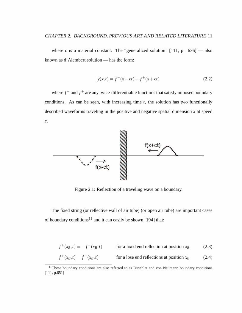
wherec is a material constant. The “generalized solution” [111, p. 636] — also
known as d’Alembert solution — has the form:
y(x, t) = f−(x−ct)+ f +(x+ct) (2.2)
wheref− and f + are any twice-differentiable functions that satisfy imposed boundary
conditions. As can be seen, with increasing timet, the solution has two functionally
described waveforms traveling in the positive and negative spatial dimensionx at speed
c.
Figure 2.1: Reflection of a traveling wave on a boundary.
The fixed string (or reflective wall of air tube) (or open air tube) are important cases
of boundary conditions11 and it can easily be shown [194] that:
f +(xB, t) =− f−(xB, t) for a fixed end reflection at positionxB (2.3)
f +(xB, t) = f−(xB, t) for a lose end reflections at positionxB (2.4)
11These boundary conditions are also referred to as Dirichlet and von Neumann boundary conditions[111, p.651]

CHAPTER 2. BACKGROUND, PREVIOUS ART AND RELATED LITERATURE12
that is, the traveling waveform reflects with a sign-change at fixed ends and without
one at open ends. This can also be interpreted as a virtual wave traveling in from behind
a rigid boundary has to match an incoming wave with a sign-change. This is depicted in
Figure 2.1.
Discretizing time of this solution with boundary conditions imposed on both ends
immediately yields a waveguide simulation for the ideal, lossless case (Figure 2.2).
Figure 2.2: Waveguide synthesis of ideal lossless string
Arbitrary bounded function shapes discretized over time are then represented as sam-
pled data points of that function at distancec∆t where∆t is the chosen discrete time step.
Advancing per time step corresponds to shifting by one memory cell per propagation
direction. Data-points reflect by copying and possibly inverting sign.
Of course in a more physically realistic situation, certain assumptions made when
deriving the wave-equation do not exactly hold. Physical strings dissipate energy and are
not perfectly elastic or perfectly thin. While intuitively all these effects happen at each
local point on the string, if exact local representation at every point is not necessary, all
losses can be accumulated (“lumped”) and modeled at one position in the model. If the

CHAPTER 2. BACKGROUND, PREVIOUS ART AND RELATED LITERATURE13
structure is seen as a filter, one can interpret that the lumped losses, bending stiffness [6,
for a review] as filters.
The classical Karplus-Strong synthesis method (Figure 2.3) can then be seen as a
waveguide synthesis method including losses. Note that the boundary reflections have
been lumped too, which, in the case of two fixed ends, correspond to a double sign
inversion which overall cancels.
Figure 2.3: The Karplus-Strong algorithm as waveguide synthesis.
The delay lines used in this model are of integer length. Hence, at a fixed time
step of1/44100corresponding to CD quality audio [155] with shorten string length, the
frequency resolution suffers. A filter modeling the fractional delay between the integer
and actual length is necessary to accommodate for accurate tuning. This is achieved by
using various filter design methods [114].
A number of modifications to the ideal waveguide have been studied to achieve
more realism. These extensions are usually instrument-specific, for instance the bending
stiffness of piano-strings [6] has little relevance for most plucked string instruments [99]
(for physical as well as perceptual reasons [96]) whereas tension modulation (the change
of tension with displacement) is more important for the latter where the strings are under
less overall tension than piano strings [199].

CHAPTER 2. BACKGROUND, PREVIOUS ART AND RELATED LITERATURE14
2.1.2 Finite Element Methods
Finite element methods are a vast field with general applications. For a very recent and
exhaustive reference see the three-volume work by Zienkiewicz and Taylor [222, 223,
224]. A review specific to finite difference methods can be found in [5].
In the computer music community, finite element style methods are used in two
settings. One is the study of musical acoustics, in the evaluation and theory-forming
of the dynamical behavior of musical instruments. Finite differencing has been used by
to study piano-strings [33, 34], bar percussion instruments [20, 35, 56], and square plates
[36, 115]. Finite element methods have been used to study tuning of bar percussion
instruments [27, 21] and the kettledrum [162]. These studies focus on accuracy and
validity and not on performance parameters relevant for synthesis.
The other setting is simulation. Ruiz studied the finite differencing of the string
equation [174]. Interest in this approach re-emerged, usually in the context of the one-
dimensional wave-equation [112, 113, 146]. Cadoz and co-workers don’t explicitly start
with model differential equations, but rather build ad-hoc networks of masses, springs,
dampers and other coupling mechanisms [30, 71, 31]. Finally, waveguide meshes were
proposed to model higher-dimensional structures [214]
The core to all of these methods is that the object to be simulated is discretized
spatially and the local interactions between discretization points are modeled. In the
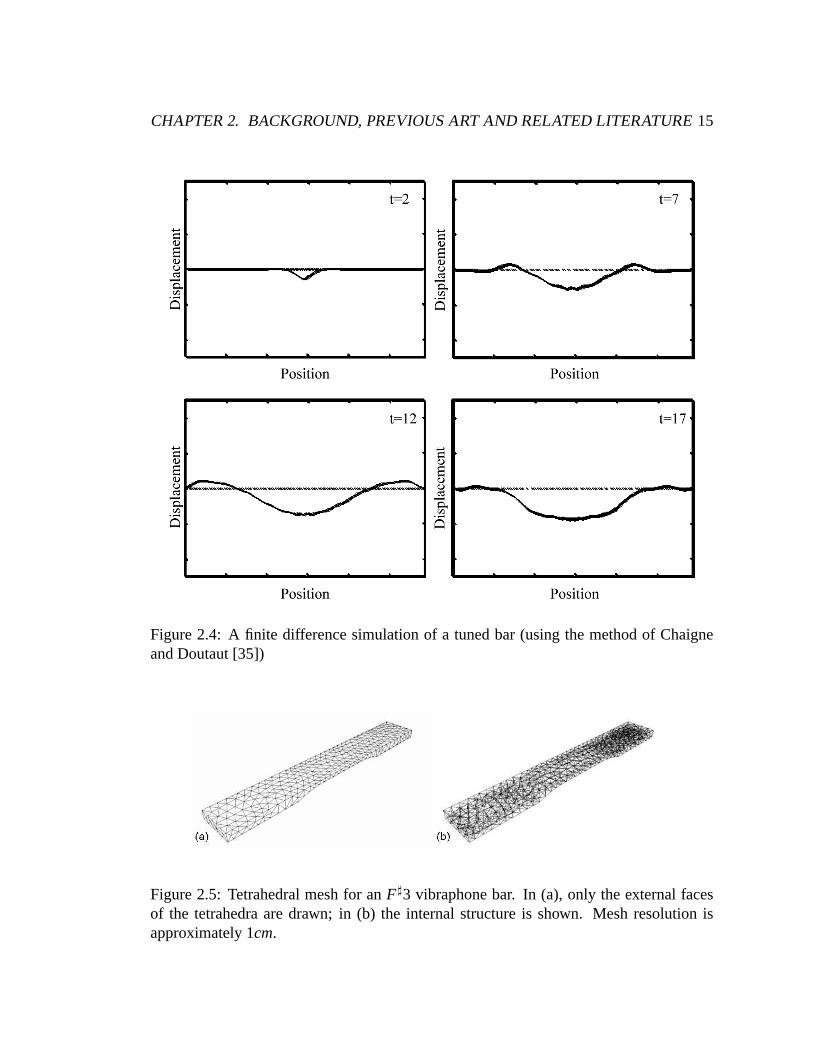
case of finite differencing, the mesh is usually uniform [5]. An example can be seen in
Figure 2.4. Non-uniform meshes are usually simulated by the more general finite element
method [222]. For a typical mesh structure see for example Figure 2.5.
The dynamics of the system that is set up is problem-dependent. However finite
element methods are usually set up as a three-stage process [222, chapter 20], a prepro-
cessing stage which takes mesh connectivity, element specification, constraints, and force
CHAPTER 2. BACKGROUND, PREVIOUS ART AND RELATED LITERATURE15
Figure 2.4: A finite difference simulation of a tuned bar (using the method of Chaigneand Doutaut [35])
Figure 2.5: Tetrahedral mesh for anF]3 vibraphone bar. In (a), only the external facesof the tetrahedra are drawn; in (b) the internal structure is shown. Mesh resolution isapproximately1cm.

CHAPTER 2. BACKGROUND, PREVIOUS ART AND RELATED LITERATURE16
Figure 2.6: Computational molecules of (a) second order and (b) fourth orderdiscretizations leading to banded entry in the model matrix of a finite element solver.
inputs and assembles them into a global matrix formulation. The second step is solution
of the system for each time-step in case of time-dependent problems or until convergence
in relaxation problems. The third stage is postprocessing which consists of extracting the
solution from the global vectors and reinterpreting as element data.
The core computational step is hence the solution of a matrix equation where the size
of the matrix is (at least in the basic case) at least as large as the number of elements. In
special cases, like one-dimensional string and bar equations on a uniform grid [35], the
formulation leads to a banded matrix (in the case of strings the band is 3 and in case of
bars the band is 5 as depicted in Figure 2.6), in which case the solution of the system is
O(NM) with N being the number of spatial mesh points andM being the width of the
band [156, pp. 50-55].
Higher dimensional and more complex domains and meshes generally don’t form
well-structured matrices, which increases the complexity. Multigrid methods [220, 22,
190, 217, 204] address this problem by solving on a coarse scale and adding refinement
steps. Other possibilities are matrix preconditioning techniques [77, pp. 532ff] and
manipulation (sparsing) [177]. In any case, usually the optimal performance is assumed

CHAPTER 2. BACKGROUND, PREVIOUS ART AND RELATED LITERATURE17
Figure 2.7: A mass-spring damper system and connected digital filter simulation
to beO(N) (for diagonal or band-diagonal matrices [156, 37]) orO(N logN) for dense
matrices [37].
2.1.3 Modal Synthesis
Modal sound synthesis refers to modeling the sound of an object as a sum of exponentially
decaying sinusoids. Physically this corresponds to simple damped harmonic oscillators,
like mass-spring-damper systems (see Figure 2.7). These second-order resonant struc-
tures have a simple representation in the form of two-pole filters, which are very efficient
to model, and hence a large number of modes can be modeled with ease.
The digital filter equation corresponding to Figure 2.7 for each time stepn is:
y(n) = a1 ·y(n−1)+a2 ·y(n−2)+g·x(n) (2.5)
The massm, spring constantk and dampingd can be used to derive the digital filter
coefficientsa1, a2 and g. In fact this digital filter is a discrete physical model of the
mass-spring-damper system.

CHAPTER 2. BACKGROUND, PREVIOUS ART AND RELATED LITERATURE18
As can be seen each filter only requires a small and constant number of multiplications
and additions and memory operations and hence the complexity of this method isO(M)
whereM is the number of modes modeled.
Models of this type have been proposed and used on a wide array of objects and
instruments [1, 219, 182, 210, 211, 208, 212].
Modal shapes can be reconstructed by sampling the surface and hence reconstructing
the modal shapes through an amplitude envelope as function of discrete spacek. Then
equation 2.5 becomes:
y(n,k) = a1(k) ·y(n−1)+a2(k) ·y(n−2)+g(k) ·x(n) (2.6)
This approach has recently been used by Pai and co-workers (see for example [208],
and note that their equation (1) is a sum of sinusoid form of equation 2.6, and a derivation
showing the connection can be found in [212]).
There are approaches which analytically derive the modal shapes for the dynamics
using transfer function methods [157, 200]. This method was also proposed to arrive at
the full solution over the whole spatial domain. By doing so, oscillation related to spatial
sampling is reintroduced and the computational complexity becomesO(NM), whereN
is the number of spatial sampling points. Hence the transfer function method is assumed
to belong to the class of finite element methods for the purpose of this discussion.

CHAPTER 2. BACKGROUND, PREVIOUS ART AND RELATED LITERATURE19
2.2 Excitations
The vast majority of sound-producing physical events as used in musical instruments
can be well-separated into excitations and a responding sounding object [165]. In a
performance sense, this relates to control of the instrument (because the excitation drives
the sound production it provides control over the production) and in a physical sense, it
relates to energy input or transfer.
This energy transfer can be classified in two ways. One is that it happens independent
of the state of the driven system (i.e. excitation and production are “decoupled” [165, p.
269]) or they are not. Then the energy transfer depends on the state of the system and
excitation and production are “coupled” (Wawrzynek classifies a similar distinction as
“driven” versus “nondriven” [219].)
While Roads emphasizes the performance aspect of this separation [165, p.269] there
is a good physical reason for this distinction affecting sound production, control and
performance.
The distinction has to do with interactions which classify as linear as opposed to those
that don’t.
2.2.1 Linear or Impulsive Excitation
The definition of a linear excitation is that the variables driving an interaction are not
affected by the state of the system that is being interacted with.
Note, that this explicitly refers to the interaction rather than the system being inter-
acted with. The system could be non-linear, meaning that it does not respond to twice
the input with twice the output, but the interaction remains unaffected. For the following
discussion I will, however, assume that the system is linear and time-invariant too. This

CHAPTER 2. BACKGROUND, PREVIOUS ART AND RELATED LITERATURE20
means that the the interactions can be divided into separate linear contributions12 and that
the system is invariant under a time-delay operation [142, p. 19].
It is easy to show that any discrete linear time invariant system can be completely
described by the system’s impulse response [142, p. 21].
In this light, a linear interaction refers to an interaction where the driving physical
quantity (for example the impact force of a strike) is, to a good approximation, unaffected
by interaction itself and hence directly relates to a digital impulse in the simulation.
In a finite element formulation this corresponds to a force functionF which is inde-
pendent of any state variables of the system.
A wide class of instruments have been modeled with their typical types of interac-
tions. The interactions which are well approximated as linear interactions are plucking,
striking with hard beaters, and certain rough-surface frictions (those where the rough
surface action is well-captured by periodic impulses) [210, 209, 211, 163, 54, 208, 212,
42, 44].
2.2.2 Nonlinear or Friction Excitation: Stick-Slip
For non-linear excitations, the independence of excitation from the state of the system
does not hold. Hence, the force function of a finite element approximation is a function
of the state of the system and weighted impulse input to discrete-time linear time-invariant
systems are dependent on the filter state.
The discussion will be limited to a class of non-linear friction phenomena called
“stick-slip” friction [3]. A particular instance of stick-slip friction is the action of a violin
bow on a bowed object (typically a string). Early work has been performed by Helmholtz
12This condition is usually divided into linearity within one input, called homogeneity or scaling propertyand linearity between multiple different inputs, called additivity or superposition property [142, p. 18].

CHAPTER 2. BACKGROUND, PREVIOUS ART AND RELATED LITERATURE21
[86], Rayleigh [159] and Raman [158], though early mentionings can be traced back
to Galileo Galilei [69, p. 331] and Chladni [40, 218]. Keller and Friedlander [101, 72]
independly developed the theoretical foundation of bowed string action that is still widely
used today in computer models [186, 133]. The friction characteristic used by them is
depicted in Figure 2.8. This basic model was subject to a number of refinements taking
into account the width of the bow [150] and more detailed knowledge of the action of
rosin on the bow [183, 184] and has been used in waveguide synthesis [180].
Cou
rtes
yJu
lius
O.S
mith
Figure 2.8: Friedlander-Keller friction diagram (from [188]).
It has been known since Chladni [40, 218] that other objects (in particular bars and
plates) can be bowed using a rosined bow. In particular this has been recently used to
study the glass harmonica [172]. Nonetheless the specifics of the musical application of
the violin bow to other systems remains largely unexplored. A notable and fascinating

CHAPTER 2. BACKGROUND, PREVIOUS ART AND RELATED LITERATURE22
example is the Chinese Dragon Wash which includes not only the friction-induced sound
production but also water waves [53, 52].
Stick-slip friction as excitation of sound is in other contexts considered undesirable.
Examples are brake noises [3, 87], propeller shaft noises of submarines [69], squeals from
train wheels [84, 82], friction noises of insects [3] and more. This lead to a large corpus
of research on friction-based oscillations [3, 69, 92, 93, 203, 123, 87] is concerned with
the damping (i.e. control) of such sounds [83, 197, 85].

Chapter 3
Theory of Propagation Modeling Using
Banded Digital Waveguides
Anybody else could have told me this in advance, but I was blinded by theory.
– Bertrand Russell1
I hear that you write poetry as well as working in physics. How on earth
can you do two such things at once? In science one tries to tell people, in
such a way as to be understood by everyone, something that no one ever
knew before. But in poetry, it’s the exact opposite. – Paul Dirac to Robert
Oppenheimer2
Junta ist totz (sic) der langen Regeln einfach zu erlernen3 – From the Ger-
man instructions to the board game Junta4
1In “The Autobiography of Bertrand Russell,” vol. 2, chap. 5, p. 288 (1967).2Attributed by Leo Moser in H. Eves, “Mathematical Circles Adieu,” Prindle, Weber and Schmidt, p.
70 (1977).3Junta is easy to learn, despite the long rules.4By ASS/Schmidt, 1986.
23
CHAPTER 3. THEORY OF PROPAGATION MODELING 24
3.1 Overview and Motivation of Propagation Modeling
for Sound Synthesis
In the real world, sound is generated through a wide variety of interactions between
objects. Some interactions can be modeled easily, using simple and efficient methods,
whereas others cannot. In a virtual world it is desirable that all interactions are captured
by real-time simulation methods. In this chapter I study and generalize propagation mod-
els to explore possible intermediate solutions between simple resonant modal methods
and slow but general finite-element methods.
3.1.1 Local Displacement to Moving Disturbance
Traditionally, when thinking of numerical simulation of elastic vibration, we are used
to describing the change of displacement in the form of partial differential equations,
which are derived from the constituent equations of general elasticity. Then these dif-
ferential equations are approximated by discretization, which creates a finite sampling
of the displacements in and on the physical objects. The finite difference operators
describe how one sampling point moves depending on its neighbors. In this approach,
the perspective of oscillation is a stationary one — the focus of observation is on the
displacement of the local data points. There is, however, a different perspective possible:
How do disturbances propagate in a medium? This question suggests keeping the focus
on the position or the behavior of the disturbance itself, rather than focusing on the local
displacements of the medium. This is the approach that is being taken in this thesis and
will be described in the following sections.

CHAPTER 3. THEORY OF PROPAGATION MODELING 25
3.1.2 Propagation of Sound in Air
Wave propagation as a way of thinking is by no means new to sound modeling. Some
acoustical phenomena strongly suggest looking at propagation directly. Imagine you want
to model an echo effect: A person calls into a valley and the call returns at various delays
of time, having traveled down and up the valley and reflected at the side and bottom
rocks. Propagation modeling of this kind is well known and widely used in simulating
room acoustics [74]. As this propagation has a finite speed, air as a medium delays the
arrival of sound . The listener does not really know or need to know the peculiarities or
details of the sound traveling down the valley and returning but only how long it takes and
how the sound changes. It does not matter when exactly a change in temperature affects
the traveling speed, but that the delay was decreased or increased. It does not matter so
much that there was a strong cross-wind in the valley as much as its effect on the heard
sound. To abstract this picture, one can see the calling as input into a propagation system
(the air confined in the valley) and the sound returning to the listener is the output (Figure
3.1).
Figure 3.1: Input, propagation system, output.

CHAPTER 3. THEORY OF PROPAGATION MODELING 26
3.1.3 Guided Waves
Air waves in tubes also propagate at a finite speed and get attenuated over time due
to losses, but because of the constraints of the tube walls, the propagation direction
is confined and or “guided.” So-calledwaveguidemodels of musical instruments use
this knowledge. It turns out that disturbances traveling on elastic strings have the same
property and that string instruments can also be modeled using the same method.
Waveguide models assume that all frequencies travel at the same speed. This is not
true for many media, in particular it is not true for solid objects of almost any material.
However, the waveguide model can be modified and extended to accommodate slight
variations in propagation speeds. Low piano strings, for instance, are thick enough so
that the bending stiffness becomes important and does introduce noticeable effects on
the sound. High frequencies travel slightly faster than low frequencies and the resulting
effect on wave shapes is called dispersion. This effect is relatively weak and can either
be modeled by spreading the reflection function [122] or by adding an all-pass filter
which introduces the appropriate propagation response [187]. If the dispersion becomes
a dominant behavior, as in the transverse oscillation of solid bars, both these approaches
becomes expensive.
3.1.4 Limits and Alternatives to Propagation Modeling so Far
So it might seem like the propagation idea is in trouble when it comes to modeling
vibration of solid objects. This is a large class of real-world objects of interest for
musical and non-musical sound simulation. In this case, we have two approaches that
don’t explicitly use the propagation idea. A very general approach is to discretize the
object in space and simulate the constituent equation that describes the interactions in
CHAPTER 3. THEORY OF PROPAGATION MODELING 27
the object using finite or boundary-element methods [135]. At present, these methods
are computationally expensive and not suitable for real-time application. A second ap-
proach uses just the modal frequencies of objects to simulate their sound. These modal
frequencies are typically derived from measurements [208] but could also be derived
from the general equations used for finite element methods. This method is efficient and
works well for all types of linear interactions. This means that the interaction can be well
described by impulsively adding energy to the system. For many complex interactions,
however, this assumption is not true. Rather the interaction does depend on the physical
state (i.e. force, velocity, displacement) of the object, like multiple bounces of interacting
objects or strongly non-linear interactions like stick-slip friction. The following section
discusses how this limitation can be overcome using propagation modeling.
3.2 A Sketch: Generalizing the Propagation Idea
We have previously proposed for one-dimensional objects that, in fact, the propagation
idea can be preserved and leads to efficient simulation [61]. Here we would like to extend
the idea to sounding objects of two and three dimensions. In later sections, we will
explain the application of this idea to bars, Indian Tabla drums, and glass harmonicas,
each being an example of one, two and three-dimensional structures, respectively.
The key point of our method is to maintain the sound propagation interpretation in
objects and use an understanding how this propagation gives rise to the sound response
of the object.
In essence there are two possible sound responses of an object to interaction:
• Resonant mode:After the wave has traveled through the object and come back,
the wave closes onto itself in its original phase. In the absence of damping, the

CHAPTER 3. THEORY OF PROPAGATION MODELING 28
energy of that frequency will be maintained while traveling on the object because
this situation constitutes “constructive self-interference.” This principle is called
the principle of closed wavetrains [47] or simplywavetrain closure.
• Anti-modal response:The traveling wave does not close onto itself in phase. The
energy will dissipate quickly at that frequency due to destructive self-interference.
Hence, there is an intimate connection between the modal response of an object to
excitation and the propagation of frequencies in the object.
To be valid, propagation modeling has to observe these two points. Sound waves
at resonant frequencies have to close on themselves in phase after traveling through the
objects and returning, or an anti-modal response occurs otherwise.
Generalized propagation modeling takes these constraints literally. The propagation
of frequency bands is modeled in such a fashion that at the wavetrain closure exactly
matches the modal response of the system and that at other frequencies the waves are
damped out quickly. A digital structure which has exactly this property is a frequency-
band-limited delay line, which closes onto itself. As described before, a delay line which
closes onto itself is a basic building block of waveguide models. We have named this
structure the “banded waveguide” [61]. However, this physical analog is valid only for
structures where waves are strictly guided: essentially one-dimensional structures like
solid bars. For higher-dimensional structures it would be more appropriate to refer to
wave-paths than wave-guides. Banded waveguides can be implemented efficiently : delay
lines have constant execution time per time step. The band-limiting can be achieved by
using a simple band-pass filter, as most applications do not require modeling the anti-
modal response precisely5. Finally, fine tuning of the length of the delay is necessary,
5A higher order filter design could be used if precision is desirable.

CHAPTER 3. THEORY OF PROPAGATION MODELING 29
especially for high frequencies. This can be achieved by adding a simple fractional delay
filter [187]. The computation time for these filters is negligible.
Figure 3.2: A single banded wave-path.BP is a band-pass filter.
The relationship between frequency and traveling speed is not unique, because it
depends both on the traveling distance and the traveling time, so knowledge of both is
necessary to maintain the proper relationship between propagation and frequency. The
additional information to remove this ambiguity can either be measured or derived from
constituent equations. When the traveling speed and the traveling length is known, the
traveling time can uniquely be calculated. If this information is not known, we can take
a good guess and use that guess in the simulation. The system spectrum will be modeled
correctly, but the response time may differ. This affects only the transient response of the
system, as the modes come in either too fast or too slow, but once the mode is established,
it physically looks no different. For non-linear interactions this means that an object may
lock to a mode more quickly or not as quickly as expected, but it won’t affect that it locks
to the mode. Hence, the result sounds and behaves qualitatively correct.
The minimal structure of a complete model consists of one “banded wavepath” per
mode of the structure. The sought physical quantity is the sum of the output of all
paths. Simplifications can easily be achieved by ignoring less significant modes, which

CHAPTER 3. THEORY OF PROPAGATION MODELING 30
is analogous to only considering the most prominent eigen-frequencies of a system in
principle component analysis. The total computational complexity depends only on the
number of significant modes of the objects, which for many real-life objects is very small,
as we will see in the examples described in the following sections.
Figure 3.3: A simple banded waveguide system.
More complex structures are possible, if details of propagation are known and deemed
necessary for improved simulation. Figure 3.4 shows two concatenated banded waveg-
uide structures to show the propagation of waves to a reflection point, the reflection
interaction being explicitly modeled and the propagation back to the start. Also note,
that by splitting traveling paths, interaction and observation points can be made different
as can also be seen in the location of the output in Figure 3.4.

CHAPTER 3. THEORY OF PROPAGATION MODELING 31
Figure 3.4: A banded waveguide system including explicit modeling of the reflection.
3.3 Description of Abstract Banded Waveguides
Banded waveguidescan be viewed in various different ways. In this section, I will present
them in their most abstract form, without additional interpretation. In the following
sections, I will then go on discussing them in various interpretations.
In the most abstract sense, banded waveguides are frequency-domain decompositions
of propagation phenomena. The complete behavior is separated into sub-domains and
the overall behavior is assumed to be the sum of contributions of each sub-domain. More
formally, banded waveguides start with the assumption that the closed frequency domain

CHAPTER 3. THEORY OF PROPAGATION MODELING 32
Ω of a propagation phenomenon can be decomposed intoN = 1. . .n sub-domainsΩn
such that:
Ω =N
∑n=1
Ωn (3.1)
The operatorF when acting onΩ has the property of returningΩn for all n and
hence will be called the domain sub-division operator. This operator may or may not be
separable into operationsFn such that:
FnΩ = Ωn ∀n (3.2)
Secondly, it assumes that within each sub-domainΩn the modeled behavior can be
separated into one or more componentsDin with i ∈ I of wave-propagation of constant
speed withinΩn and zero or more componentsH jn with j ∈ J which don’t observe that
property.
Thirdly, each sub-domain component structure (the set of allDin,H
jn, which may or
may not includeFn, for a particularn) or the sum of all substructures (includingF for
separation and the summation for combinationΣ6) is cyclic, in general. That is, the
domainΩ and also the domainsΩn each have their boundaries connected.
The cyclic domains, with or without the equation 3.1, can be seen in Figure 3.5.
6May also be denoted byF−1. TheΣ is preferred as it corresponds to the definition of recombination inequation 3.1

CHAPTER 3. THEORY OF PROPAGATION MODELING 33
Figure 3.5: Abstract depiction of the cyclic property of domains and their decompositions
According to the above definition, the minimum banded waveguide consists of domain-
decompositionF , and a set of constant-speed wave-propagatorsDn, one per sub-domain
Ωn.
3.3.1 Notation
As a notational convention7, Din and H j
n refer to abstract components (one could also
think of them as continuously defined within the domainΩn). An indexω in parenthesis
following the components denotes the frequency response of the component, i.e.H(ω) jn
usually withω∈Ωn8. The z-transform [194, 142] will be denoted caligraphic script letter
followed byz in parenthesis byH (z) jn. In all instances, indices and parenthesis may be
omitted if properties are discussed which are true for all instances of a component, that is
7See also [48, section 10.2] for a related symbolic notation. I chose a different notation to relate moreclosely to filter theory and also because I would like to capture more than just the transition dynamics withthis notation.
8Note that in cases of non-exact decomposition into sub-domains this may be loosened toΩ, that is thefrequency over the whole domain may be considered.
CHAPTER 3. THEORY OF PROPAGATION MODELING 34
H describes properties of allH (z) jn with n = 1. . .N and j = 1. . .J. Also an index may
be dropped if the size of the index set is one. For example, ifN = 1 then we writeH (z) j .
OperatorΣ should usually be read as summation over indexn corresponding to equa-
tion 3.1.
3.4 Banded Digital Waveguides as Filters
The abstract model described in the previous section can readily be turned into a digital
filter model by assuming that the domainsΩ andΩn are discretized and that all operators
are discrete linear operators. In fact, we’ll assume uniform discretization of the domain
or a mapping to a uniform discretization. Hence all structures involved are indeed linear
time-invariant digital filters [142].
From the definition of the properties of the operator in the previous section, a number
of properties of the digital filters can be inferred. This connection will be discussed in the
following sections for all operators.
3.4.1 Domain Decomposition Filtering
Though the filter structure for achieving domain decomposition is quite general, I will,
in this thesis restrict the considerations to single-rate systems. Hence time-domain deci-
mation as in decimation filterbanks and wavelets [204] are not considered. While in the
abstract notion of banded waveguides there is little motivation to this restriction, I will
justify this decision when discussing physical interpretation of the structure (section 3.6)
and computational performance (section 3.11).
While, per se, in the abstract definition, the functional form of the propagating wave
of the decomposition is not prescribed, we will assume that a sum of sinusoids (that is

CHAPTER 3. THEORY OF PROPAGATION MODELING 35
a Fourier basis) is a good basis. Hence any frequency band decomposition observes this
assumption and the definition of section 3.3.
F (z) then could be any type of bandpass filterbank or a discrete Fourier transform,
and F (z)n would correspond to individual bandpass filters or bins in a discrete trans-
form. Which particular structure should be chosen depends on the desired decomposition,
which in turn will depend on the application and interpretation of the structure. This
choice will be discussed in sections 3.5–3.10.2
3.4.2 Constant-Speed Wave Propagation Filter: Delay line
The decomposition chosen in the previous section separates into Fourier subdomains,
so Ωn can be read as a discrete band-limited frequency domain. As by definition, the
propagation operatorsDn propagate waves at constant speed independent of frequency
content, the corresponding filter has to delay all frequencies by the same amount within
the frequency band defined by the respective subdomainΩn. One operator which satisfies
this condition can be written by the z-transform [194, compare p. 69]:
D(z)n = z−d with d ∈ R (3.3)
whered is the delay in samples per time-step. I will limit myself to this operator in the
following discussion. In particular the delay operator can be split into two parts, a delay
part of integer length (we will choose the largest integer less than or equal tod) di and a
non-integer or fractional delay partdf :

CHAPTER 3. THEORY OF PROPAGATION MODELING 36
D(z)n = z−(di+df ) with di ∈ N anddf ∈ [0,1) ∈ R (3.4)
D(z)n = z−di z−df (3.5)
The integer time delay is simply a queue9 of length di . The fractional delay is a
sub-sample delay operator whose practical realization is reviewed in [114].
3.4.3 The Perturbation Filter
By definition in section 3.3, the operatorsHn are not restricted, except that they contain
behavior that cannot be modeled by the propagation operatorsDn with the sub-domain
Ωn. The only real restriction ofHn is that it operates within the sub-domain and hence can
be any filter structure with this condition. Here we will add another restriction, namely,
that ofH (z)n being a linear time-invariant filter. The meaning of this restriction and its
possible loosening will be discussed in the context of the interpretation of the concrete
interpretation ofH (z)n in application. The same is true for the actual form of the filter
which again is highly dependent on the application and interpretation and hence will be
revisited in sections 3.5-3.10.2.
3.4.4 Domain Reconstruction Filtering
Domain reconstruction can either be derived from the abstract combination equation 3.1,
where the reconstruction is simply the sum of the sub-domains, or one could also see the
reconstruction as the inverse to the decomposition operatorF (z), that is a reconstruction
filterbank or an inverse Fourier transform.9More precicely a queue with first-in, first-out property.

CHAPTER 3. THEORY OF PROPAGATION MODELING 37
3.5 Banded Digital Waveguides as Phase-Corrected Modal
Synthesis
As discussed in the background chapter in section 2.1.3, modal synthesis simulates the
decaying modal frequencies of sounding objects using either additive sinusoidal synthe-
sis or resonant filterbanks. The advantage of the latter is that it has a direct physical
interpretation as equivalent mass-spring-damper oscillators and hence force inputs can
be converted conveniently into appropriate digital units.
Modal synthesis is a degenerate form of the banded waveguide structure, lacking
closed loop delaysDn or perturbation filtersHn. Hence, the domainΩ of this structure is
simply a point. The total model equation is:
F ·F−1 (3.6)
In particularF is a resonant filter bank andF−1 is the sum over all the output of the
filter bank.
Compare this structure with the structure of the decomposed domains of an abstract
banded waveguide (Figure 3.5), which can be symbolically written as:
F · [D1 · · ·Dn] ·F−1 (3.7)
where[ ] implies that the operatorsDn are applied to the sub-domains created by operator
F .

CHAPTER 3. THEORY OF PROPAGATION MODELING 38
The operatorsDn are all-pass filters and hence only modify the phase of the signal
within each frequency band and as theF−1 is only a linear combination of the separate
bands, the difference between modal synthesis and banded waveguides of the form of
equation 3.7.
F ·D ·H ·F−1 = D ·H (3.8)
That is, there is only one subdomain which is equal to the original domain (hence both
the decomposition and reconstruction operators are unity) and there is only one chain of
propagation.
3.6 Banded Digital Waveguides as Generalized Digital
Waveguides
Digital waveguides as introduced in section 2.1.1 have the following abstract notation:
D1 ·H1 ·D2 ·H2 · · ·D j ·H j (3.9)
or, if all H j can be commuted it has the abstract “Karplus-Strong” equation:
D ·H (3.10)

CHAPTER 3. THEORY OF PROPAGATION MODELING 39
As can be seen the digital waveguide structure simply is a banded waveguide structure
without domain-decomposition (which is equivalent to saying over one sub-domain,N =
1).
3.7 Banded Digital Waveguides as Multi-scale Numeri-
cal Method
The abstract definition of the banded waveguide structure as introduced in section 3.3
does not directly specify a physical interpretation of the structure. It does contain a notion
of delay which in a physical sense does link to a notion of time. Assuming thatD∗n is
the total accumulated delay operation of the subdomainsΩn then the original definition
leaves undefined the relationship between these delays. The case of equal delay of all
sub-bands has been treated in the previous section and simply corresponds to the standard
digital waveguide structure. In this case, digital waveguide filters also carry a physical
interpretation of space. The d’Alembert solution describes the propagation of waves
along the spatial extension of a string. Correspondingly a unit time delay∆t represents
a unit of spatial length∆s, which can be calculated from the time-delay via the wave-
velocityc (compare to equation 2.1):
∆s= c·∆t (3.11)
In the more interesting case of sub-domain having distinctive delays, if a subset is
interpreted to follow the same spatial trajectory of lengthl then, given a defined temporal
unit ∆t, the speedcn within each sub-domain is:
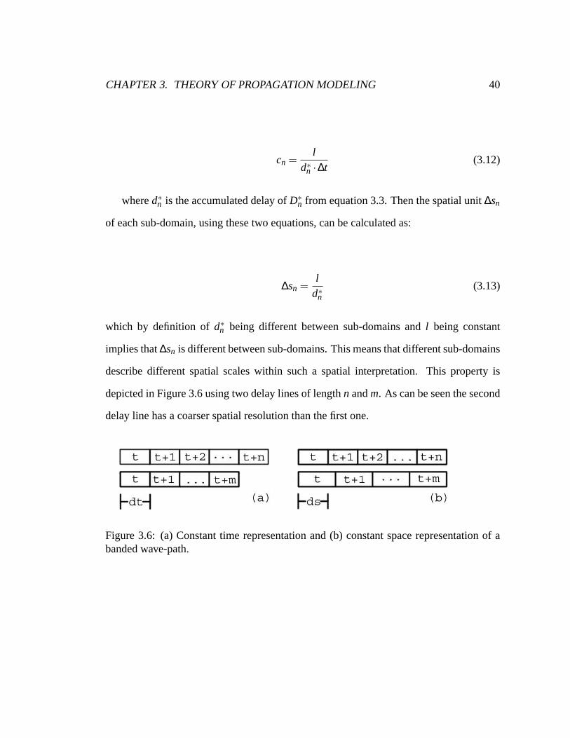
CHAPTER 3. THEORY OF PROPAGATION MODELING 40
cn =l
d∗n ·∆t(3.12)
whered∗n is the accumulated delay ofD∗n from equation 3.3. Then the spatial unit∆sn
of each sub-domain, using these two equations, can be calculated as:
∆sn =l
d∗n(3.13)
which by definition ofd∗n being different between sub-domains andl being constant
implies that∆sn is different between sub-domains. This means that different sub-domains
describe different spatial scales within such a spatial interpretation. This property is
depicted in Figure 3.6 using two delay lines of lengthn andm. As can be seen the second
delay line has a coarser spatial resolution than the first one.
Figure 3.6: (a) Constant time representation and (b) constant space representation of abanded wave-path.

CHAPTER 3. THEORY OF PROPAGATION MODELING 41
3.8 Banded Digital Waveguides as Discrete Asymptotics
Simulation
The principle of wavetrain closure states that a mode will occur when a traveling wave
after following some path closes onto itself and the wave is in phase with itself at the
closing point of the path. Otherwise no mode occurs. In essence, the mode comes about
as constructive interference of a traveling wave with itself.
3.8.1 Previous Work: Traveling Wave Solutions
The idea of constructive and destructive interference of linearly independent traveling
waves is a long known phenomenon, that has explained many observations involving
waves, like diffraction patterns.
The d’Alembert solution of the ideal finite string is maybe the first specific example
of a description of a dynamical system that follows the wavetrain closure principle.
Extension of this type of description to other dynamical systems happened in the
middle of the last century independently in the acoustics community and the mathemat-
ical physics community. Among the acousticians who developed the idea were Mead
[124, 125, 126, 127], Cremer and Heckl [47]. The focus was primarily on bar structures
but attempts were made to extend to square plates.
Another line of research again comes from the eminent scientist Joseph Keller who
is in the community mostly known for his work on theoretical non-linear friction be-
havior of the bowing violins [101] and the friction characteristic is generally known as
Friedlander-Keller diagram [188] (it has been simultaneously and independently studied
by Friedlander [72]).

CHAPTER 3. THEORY OF PROPAGATION MODELING 42
Keller studied asymptotic approximations to dynamical systems, in particular optics
and quantum mechanics. In joint work with Rubinow, he proposed that the method could
also be used to find eigenvalues of dynamic structures [104]. The idea is that the dynamics
of structures can be well approximated by studying the behavior of traveling wave rays.
This is similar to using principles of geometric optics to describe general optical wave
phenomena asymptotically, as Keller did in his geometric theory of diffraction [102].
Keller and Rubinow showed how, using their approach, circular membranes and elliptical
domains can be solved. They also showed how whispering gallery modes and bouncing
ball modes can be derived on more arbitrary two-dimensional domains. Though the
theory of asymptotics has found a lot of interest and applications in many fields [103],
the study of structural dynamics as relevant for many musical instruments has been quite
limited, the exception seems to be work by Chen, Coleman and co-workers who study the
effect of bending stiffness using Keller’s approach [39]. In less direct form, this approach
has seen extensive interest in the mathematics and physics community. Finding a closed
path on a closed domain of some shape can be seen as a billiard ball rolling on a surface
and bouncing off the walls and returning to its starting position. In this setting, billiard
balls are said to be on periodic orbits, and the task is to find them. On the convex domain
this has been extensively studied by Birkhoff and others [109].
Traveling wave methods are studied and used in a vast number of different fields.
Connected theories have been developed in pure and applied mathematics with various
motivations. Among them is approximate and exact solutions of ordinary and partial
differential equations, even when they may not be integrable [139, 215, 68] often mo-
tivated by equations that arise in classical mechanics [205, 108] or quantum mechanics
(the asymptotic approach is usually referred to as “semiclassical mechanics” for the limit
of the asymptotics establishes the correspondence between classical results and quantum

CHAPTER 3. THEORY OF PROPAGATION MODELING 43
mechanical formalism) [103, 25] and has been instrumental in both areas (and others)
in the study of chaos [48]10. Even in simple integrable dynamical systems, a traveling
wave Ansatz usually has points where a unique solution cannot be derived (referred to
as caustics, see also Appendix A). Solutions at and in the neighborhood of these points
are sought via connection formulas [13] and special functions [139, 14], as topological
projection [129, 110]11 and via hyperasymptotic expansions [78, 24, 89] [38, for a de-
tailed review including the connection to rays in two-dimensional elasticity dynamics].
Asymptotic methods find applications in electromagnetics [23] and seismology [50].
3.8.2 Previous Work: Numerical Traveling Waves
Numerical simulation based on discretized traveling waves for the wave-equation was
accidentally discovered by Karplus and Strong and was quickly recognized to be a very
efficient method of simulating the dynamics of strings and air-tubes. This method is
called “digital waveguide filter method” [187]. It is an accurate simulation for ideal
strings and other idealized waveguide systems that are basically one-dimensional. It
can be seen as discrete implementation of the d’Alembert solution of the governing
equation. However, it is probably much more intuitive to consider the d’Alembert so-
lution a proper dynamical description rather than a solution. Deviations from the ideal
are then introduced while maintaining the traveling wave picture. Local damping and
dissipation are described as damping and dissipation of a traveling wave along its path and
at boundary reflections. Stiffness is introduced as a change in propagation characteristic,
and so on. If the perturbations from the ideal case are small, this works quite well:
10The usefulness of asymptotics in studying phenomena has also been the focus of interest withinthe philosophy of science [10] especially as a way of reasoning between different levels of details withquantitatively different behavior. For a short and popular account see [15, 73].
11A very brief but lucid review of the the connection between “Lagrange manifolds” and caustics throughprojection can be found in [58].

CHAPTER 3. THEORY OF PROPAGATION MODELING 44
the digital waveguide filter method is widely successful for many musical instruments.
Digital waveguide filters have a number of additional advantages over finite differencing.
Stability considerations are much more simple and intuitive, as in the case of waveg-
uides, the deciding factor is simply whether the loop gain is below or above unity. The
transportation within the waveguide is “numerically safe” as disturbances are transported
multiplication-free, i.e. they are simply copied and hence even a gain of unity yields a
perfectly sustained oscillator which is difficult to achieve with “algebraic propagation”
involving multiplications and additions, as in the case of finite differencing. The key
benefit though is that, in addition, or rather because of this condition, waveguides can
be implemented with constant numbers of operations (read, write and pointer updates)
independent of the length and hence the spatial sampling, whereas finite differencing
schemes depend on the spatial sampling resolution.
Figure 3.7: A digital waveguide filter.
An interesting note to make is that we are, in fact, using an asymptotic method that is
valid for the short wave-length limit and ceases to be strictly valid for long wavelengths.
One might hence be tempted to conclude, that all this should not work. Surprisingly
though it has repeatedly noted, that even for the long wavelength solutions (that is the low
eigenmodes), the asymptotic method performs well [104, 178]. In specific cases, like the
d’Alembert solution for the wave equation, the “asymptotic” traveling wave Ansatz is in
deed exact.

CHAPTER 3. THEORY OF PROPAGATION MODELING 45
3.8.3 Discrete Asymptotic Simulation
The relationship between banded waveguides and traveling-wave, ray or Wenzel-Kramers-
Brillouin (short WKB) methods12 can be seen using the following line of reasoning.
Starting with the minimal banded waveguide equation 3.7 and letting the number of sub-
domains go towards infinity, one arrives at a function defined inω ∈ R+0 over the initial
domainΩ:
d(ω) = limn→∞
F · [D1 · · ·Dn] ·F−1 (3.14)
(3.15)
d(ω) can then be interpreted as a continuously (though not necessarily smoothly) defined
function of delays over the domain. Writing the delay using an exponential propagator
and interpretingω as frequency one gets:
e−i·d(ω)ω (3.16)
This form corresponds to the Keller-Rubinow-form of the WKB-asymptotics found
in their seminal treatment of oscillatory problems in two dimensions [104, eq. (3)]
describing the sum of all paths:
u =N
∑j=1
ei·kSj[A j +O(1/k)
](3.17)
12For a glossary of terms used in the asymptotics literature also refer to Appendix A of this thesis.

CHAPTER 3. THEORY OF PROPAGATION MODELING 46
If the the loop described by the domainΩ is interpreted as two parts, a forward
propagating half and a backward propagating half, then this becomes:
e+i d(ω)2 ω +e−i d(ω)
2 ω (3.18)
This form corresponds to the oscillatory (that is imaginary part) of the Olver-form
[139, p. 190, eq. (1.02)] of the WKB-asymptotics13:
w∼ A·ex√ f (x)+B·e−x
√ f (x) (3.19)
Hence, in the limit of infinite sub-domains, banded waveguides can be considered
equivalent to WKB-asymptotics, and, in the finite case, it is a finite approximation of
it. It should be noted though that this does not imply that the method is necessarily just
approximative to any dynamics. In the case of the wave equation the d’Alembert solution
of the exact dynamics, the traveling-wave Ansatz are exactly equivalent (derivation of the
d’Alembert solution can be found in many standard textbooks, for example [111, chapters
11.3 and 11.4]).
The correspondence between WKB-asymptotics and banded waveguides is of imme-
diate relevance because the known results of properties of asymptotics, ray and traveling-
wave methods become immediately relevant to the mathematical and physical under-
standing of banded waveguides. This correspondence will become relevant in the follow-
13Which Olver calls LG approximation, see Appendix A.

CHAPTER 3. THEORY OF PROPAGATION MODELING 47
ing section discussing banded waveguides in dimensions higher than the one-dimensional
line-model14
3.9 Banded Digital Waveguides in Higher Dimensions
In previous sections, I have introduced a spatial interpretation (section 3.6), and the
domain composition has been given a spectral interpretation (section 3.4) of the abstract
banded waveguide model of section 3.3. However, the domain separation of operatorF
can also be interpreted geometrically. Then operatorF can be interpreted as:
FmΩ = Ωm (3.20)
with Ωm being geometric sub-domains, which in turn each can be decomposed into
spectral domains:
FnΩm = Ωmn ∀m (3.21)
For the remaining discussion, the geometric sub-domains will be assumed to be
ray or line domains, and hence the discussion that has previously been carried out in
one dimension can be interpreted as applying to the one-dimensional trajectory of that
domain.14Dimension here refers to the number of spatial dimensions of the dynamical system under
consideration or, equivalently, the number of independent spatial dimensions in the constituent differentialequations describing the dynamics. The time and possibly orthogonal deflection dimensions are excluded.

CHAPTER 3. THEORY OF PROPAGATION MODELING 48
3.9.1 Previous Work: Single-band Multi-path or Multi-dimensional
Models
Waveguides have been used in higher dimensions under a ray-casting paradigm. This
work mostly relates to work in room reverberation algorithms as already mentioned in
section 2.1, where delay-lines were introduced. Not all works in the field that use delay-
lines use them beyond a listener-receiver path description [90, p. 38, for example]. The
use of multiple connected feedback delays has been introduced by Stautner and Puckette
[191] and is now generally referred to as feedback delay networks (FDN) [170, and
references therein]. In the early work of Stautner and Puckette, the delay-paths were
associated with channels and only loosely associated with the geometry of the room,
though the association of geometry to room response has been introduced by Allen and
Berkeley [12, see p. 183-185 for a brief review]. The “room of mirrors” idea behind their
“image” or “image-source” method describes how a reflected source is equivalent to a
mirror image acting as a source through the reflected wall. This topological mapping of a
reflected path to an unreflected path corresponds to the construction of a resonant torus as
introduced by Keller and others [104, 25]15 (see section 3.9.2). The connection between
resonant response of a geometric enclosure and its shape has been realized in this context
by Rocchesso and studied in the case of a rectangular box[166, 170] and sphere [167].
An alternate approach to multi-path feedback delay models can be found in the lit-
erature of physical models for string instruments. Until recently, the focus has been on
studying physically separate but coupled structures like coupled piano strings [8, 9, 6] or
sympathetic strings in plucked string instruments [99]. Here two separate paths couple
at some point. These paths are geometrically independent otherwise. A more interesting
15I’m unaware that this connection has previously been pointed out.

CHAPTER 3. THEORY OF PROPAGATION MODELING 49
recent example is the detailed modeling of the action of a bow on a string as presented by
Serafin and Smith [180]. This work showed that strings are not ideally thin but have in
fact finite thickness. Torsion in direction of the bow is introduced though torsional waves
in a linear string traveling independedly from transverse waves. Hence Serafin and Smith
arrive at a two-path waveguide model with one path for each wave type. In fact, a four
waveguide model has been suggested by Smith to implement waves in two orthogonal
planes for transverse oscillation, longitudinal waves and torsional waves [187].
3.9.2 Topology of Resonant Paths
In general, the problem presents itself in the form of a given geometric shape that is
responsible for the sound-generating dynamic (e.g., the shape of the membrane of a
drum) and by ray-casting on that shape, finding closed paths which then correspond to
eigenfrequencies. This is a very general problem that is still under intensive investigation
(for detailed pointers into review literature I refer to Appendix A). Here I will confine
myself to 2-dimensional discussion of square and circular domains. There two are fully
treated domains in Keller and Rubinow’s seminal paper on the subject [104]16. A more
contemporary and generalized treatment of the subject not confined to these particular
domains and dimensions can be found in [25, p. 78 ff.].
For simplicity we will assume just the finding of a closed path and will ignore the
propagation dynamics in this treatments.
Taking a rectangular domain, we assume that the behavior of the boundary of the
domain is complete geometric reflection. Starting of with a family of parallel rays shoot-
ing of at some angle, geometric reflection just means an inversion of the travel direction
normal to the boundary.
16The derivation has been repeated in many places, for instance [103, 39].

CHAPTER 3. THEORY OF PROPAGATION MODELING 50
(a) Reflections of a single ray (b) Type of Reflections for ray family
Figure 3.8: Reflection of a ray at the boundary
This behavior is depicted in Figure 3.8. Figure 3.8 (a) shows the first for reflections of
a ray starting with the configuration in the lower right corner and going around counter-
clockwise. Figure 3.8 (b) shows the same general behavior for a whole family of rays.
This picture should be interpreted as states rather than as actual ray paths, meaning that
there are four possible propagation configurations that change depending on reflections at
the boundary. Any family of rays with an angle different than90 will eventually reflect
and change directions. As a ray propagates through the domain it can reflect many times
until it closes onto itself but it still can only be in one of these configurations. Up-down
reflections are cyclically repeated as well as left-right reflections17. As is widely known
in signal processing, an open infinite domain with regular repeating substructure (e.g.
periodic sampling) can be mapped onto a closed circular domain (e.g. the z-transform of
a periodically sampled signal) [194, chapter 11]. The same holds here, though there is
17This resembles the familiar picture of alternating configurations of image-sources for increasing ordersof reflections in the image-source method. For a related depiction see [12, Figure 4.55, p. 185].

CHAPTER 3. THEORY OF PROPAGATION MODELING 51
repetition in two dimensions, hence the circular folding has to happen along both axis.
The first folding turns the two-dimensional sheet into the surface of a cylinder by gluing
the top and the bottom edge together and the second folding merges the ends of the
cylinder to form a torus (see Figure 3.9).
Figure 3.9: Resonant torus of EBK quantization of two-dimensional closed paths.
More generally any integrable system can be brought into the form of anN-torus
embedded in a2N-space by canonical transformation [25, p. 79 ff].
The torus structure has an intuitive appeal as it highlights that there are two topo-
logically independent dimensions that lead to closed curves. In the 2-torus case the first
follows along the outer rim to close onto itself and the second follows the radius of the
thickness to close onto itself18. A general path will wind around both dimensions (and
hence the related numbers are sometimes called “winding numbers” [48]) to close back
onto the same position on the torus. It also illustrates that the actual starting position
18Hence authors describing two-dimensional domains often use two-number labelings to identify closedpaths. For an example in the square case see [154], for one on circles and circle-segments see [161].

CHAPTER 3. THEORY OF PROPAGATION MODELING 52
does not matter due to the symmetry of the structure which justifies the initial treatment
of families of rays rather than rays with specific positions. Finally, as the surface area
on the torus is the same as the area traveled on the original domain, short and long
closed path configurations can be intuitively observed. For instance if the angle is very
flat with regards to one topological dimension, then the path will have to wind around
this dimension many times before having traveled around the other dimension once.
Finally it can be immediately seen that closure can only occur if and only if the ray has
traveled through an integer number of windings in all topological dimensions (because if
a winding number in a dimension is not integer the winding is incomplete).
This yields the closure condition, which by requiring integer solution, and by attribu-
tion to early contributions to this technique by Einstein, Brillouin and Keller is usually
called EBK quantization.
We are interested in total ray length and its relationship to the frequency of standing
waves, but we have so far ignored the effect of the boundary.
Classical Dirichlet boundary conditions correspond to a sign inversion in the ampli-
tude, which in turn can be written as a phase-contribution ofπ because:
ei·π =−1 (3.22)
The principle of equal phase closure demands that the phase is single-valued after one
round-trip on a closed path. If∆Sdenotes the change in phase, then it can be written as:
∆S−µ· π2−b·π = 2π ·n (3.23)

CHAPTER 3. THEORY OF PROPAGATION MODELING 53
for all n in N+0 , which leads to the common form of the quantization rule:
∆S=(
n+µ4
+b2
)·2π (3.24)
whereµ is called the Maslov index, which counts the number of touched turning points
inside the domain (also called caustics, see Appendix A), andb is the number of Dirichlet
boundaries reached.19 In the case of the rectangular domain, there is no caustics, and
henceµ = 0, and there are multiple of two reflectionsb. The caustic will be revisited in
the case of the circular domain.
Returning to the two-dimensional case described by the torus, this quantization rule
must hold for both dimensions. Rescaling the quantization condition by the path-length
2· ln (the domain is transitioned twice for each winding) and using the relation:
f =cl
(3.25)
and using the triangle inequality to calculate combined path contributions we get:
f =c2·(
m12
l12 +
m22
l22
)(3.26)
wherec is the speed of the traveling wave andl1 andl2 are the dimensions of the rect-
angular domain.m1 andm2 are positive integer quantization numbers. This corresponds
to the classical solution of the square plate [132, p. 205].
19Note that some authors include the contribution ofb in µ.

CHAPTER 3. THEORY OF PROPAGATION MODELING 54
3.10 Theory to Application: Use of Banded Waveguides
With all this theoretical description, the question remains, how practical synthesis meth-
ods can be achieved using it. In other words, how are the components of the theory
described in previous sections practically combined. First, I will talk about practical
aspects of reaching implementations of simulations from actual physical instruments
through the theory so far discussed. Then I will mention that the application does not
necessarily require the physical interpretation of the previous section.
3.10.1 Physical Simulation
Figure 3.10: Relationship of geometry and dynamics to modes.
If the goal is to arrive at the simulation of actual musical instruments or physical
but non-musical sound production mechanisms, then the question remains, how one
arrives at specific implementable structures (section 3.4) from the theoretical approach
to describing the dynamic (sections 3.8 and 3.9).

CHAPTER 3. THEORY OF PROPAGATION MODELING 55
The connection between geometry and dynamics and modes as primary components
of sound production is summarized in Figure 3.10.
In fact, the connection between components in Figure 3.10 can follow two directions.
First, if following the direction of the arrows, this corresponds to a construction of a
simulation from complete dynamical and geometrical description. Then the tasks are:
• Find periodic orbits.
• Identify boundary conditions and turning points and their phase contribution to
periodic orbits.
• Find wave propagation speed characteristics.
However, this is not necessarily the most practical approach. Finding periodic orbits
can be difficult, and the theoretical dynamics of a complex instrument may not be known.
Hence it may be difficult to find the wave propagation speed characteristics. Finally this
construction is not precise.
More realistically, if the physical instrument is available, certain parameters can be
measured. Other parameters may be known only approximately. Thirdly, not a complete
construction may be desirable.
In this context, the relationship between measured modes and theoretically constructed
modes is of interest. As said, the theoretically constructed modes are approximate. The
measured modes are, however, precise within measurement accuracy. The proposal
is, to tune closed wave-paths to the precise frequencies. Then, the deviation between
approximate theoretical, exact theoretical, and actual behavior is bridged by introducing
the theoretical deviation from the measurement in form of a path-length correction to the
theoretical path.

CHAPTER 3. THEORY OF PROPAGATION MODELING 56
3.10.2 Application as Non-physical Entities
The abstract structure, and even the filter interpretation thereof, does not necessarily need
a physical interpretation. In this case, banded waveguides can be seen as a purely ab-
stract synthesis methods with certain properties. The choice of parameters then becomes
aesthetically motivated rather than physically.
Here I only want to mention one example of non-physical application of this structure
that was discovered by accident. If the output of the reconstruction operator is numeri-
cally integrated (accumulated sum), and the appropriate “physical” interpretation of the
result of reconstruction would have been displacement, one arrives at a quantity that is not
properly physically informed. If this integrated displacement is then fed into a standard
bowing interaction model, rich, chaotic sounds can be produced in a stable manner using
this method.
3.11 Performance and Critical Sampling
The performance of banded waveguide synthesis is defined by the behavior of the various
building blocks. In general, the delay operator for integer sample delay can be cheaply
implemented using circular buffers (as mentioned already in section 2.1). In fact, the
performance is independent of the length of the delay and henceO(1). The remaining
parameters defining the computational complexity of the algorithm is the number of sub-
domainsn, the number of separate delay and perturbation blocksi and j.
Hence a driving parameter for the performance is the number of non-delay blocks that
are incorporated in the model.
In fact, the asymptotic WKB ansatz is equivalent to neglecting coupling of in- and
outgoing waves [32]. The interplay between precise differential equations, couplings

CHAPTER 3. THEORY OF PROPAGATION MODELING 57
(also referred to as scatterings) and discrete traveling wave approximations has been ex-
tensively studied by Bilbao [18], though the treatment of scattering in digital waveguides
has long been known [188]. Hence one critical area for performance gain is the process of
deciding when neglecting local scattering in a dynamical system is a good approximation
or not (physically and perceptually).
Finally, the implementation of the domain decomposition, perturbation filters and
fractional delays also affect performance.
In this thesis I do not consider decimation in time for sub-bands. This is justified
by the realization that the critical performance improvement fromO(M) to O(1) (where
M is the spatial sampling) has already been achieved and that the computational load
(i.e. the constant inO(1) of time-stepping a delay line is very small). In the same vein,
inexpensive second-order bandpass filters can be used for domain-decomposition making
this method overallO(N), whereN is the number of modeled subdomains with a small
multiplicative constant only. Whether a trade-off with decimation and interpolation op-
erators versus sub-domain time-stepping yields significant gains remains to be explored
(see section 7.6.3).
3.12 Interaction Models
Physical interactions usually take place on the whole domainΩ. Hence either at in-
teraction points the whole domain has to be reconstructed or the interaction needs to
be translated into contributions to each sub-domain. If the latter is a choice depends
whether or not the interaction implies local scattering. In general, scattering should be
assumed for non-linear interactions and may be absent for linear ones (see section 2.2).
The implications will be discussed by example in chapter 4. Here it should only be

CHAPTER 3. THEORY OF PROPAGATION MODELING 58
mentioned that in case of modeling the contribution separately to the various spectral
sub-domains implies contributions to spatial samplings of different scales (as described
in section 3.7), and hence the contribution has to follow the same scaling.
3.13 Conclusions
We introduced propagation modeling using banded waveguides to the spectrum of meth-
ods to simulate sounds of objects. The guiding question with regards to this and other
methods is: What is the least amount of information we have to consider to get the
desired result? The propagation idea allows for significant reduction of complexity and
dimensionality while allowing for retaining essential features. It allows for complex, non-
linear, yet natural interactions which cannot be modeled by other comparably efficient
models. It does this at the price of making a direct geometric interpretation specific and
potentially difficult.

Chapter 4
Applications of the Banded Digital
Waveguides
Grau, teurer Freund, ist alle Theorie,
Und grun des Lebens goldner Baum1. – Johann Wolfgang von Goethe2
Few things are harder to put up with than the annoyance of a good example.
– Mark Twain 3
Trust me, it sounded good before I improved the model. Now it sounds more
realistic.
In this chapter I will discuss application of the theory of banded waveguides to par-
ticular musical instruments. In general the progression will be an increase in spatial
dimensionality. In addition, experimental data will be presented to evaluate simulations.
1All theory, dear friend, is gray, but the golden tree of actual life springs ever green.2In “Faust” pt. 1 (1808) according to [147, p. 309, q. 5]3“Pudd’nhead Wilson,” chap. 19 (1894) available online athttp://www.cs.cofc.edu/˜manaris/
books/Mark-Twain-The-Tragedy-of-Puddnhead-Wilson.txt and according to [147, p. 706, q. 23]
59

CHAPTER 4. APPLICATIONS OF THE BANDED DIGITAL WAVEGUIDES 60
4.1 1-D Case: Rigid Bars
Bowed bar percussion instruments have found increasing interest and application in musi-
cal composition and performance in recent years. However, the excitation of a sustained
oscillation of a bar by means of a rosined bow for musical purposes has not yet been
studied systematically.
So far research on bar percussion instruments has focused on the issue of tuning by
removing material at various locations along the bar [143, 20, 149, 27], the influence
of the resonators on the vibrating bar and the radiated sound [20, 56], and the effect of
striking excitation using mallets [35]. Material properties have also been studied [29, 88].
Numerical simulations use either finite difference [20, 35, 56]4 or finite element methods
[143, 27, 21]. Summaries and reviews of the research on bar percussion instruments are
available [131, 171, 70]. When the sound of bar percussion instruments is synthesized
for real-time performance using electronic sound generation, the above mentioned finite
difference and element methods lack the necessary efficiency on current hardware to
be appropriate. Hence, current techniques only model the modes of the system, using
modal filters [219, 42] or additive sinusoidal synthesis [182, 210] ignoring the modal
shapes. Hence, the notion of physical shape and interaction is lost, and a direct way
to use these approaches for bow interactions is not possible. In essence, the spatial
dynamics is removed by replacing the actual physical system by an equivalent mass-
spring system which models the same modal response. However, the dynamics (in
particular the propagation of disturbances) of the original system is lost. Hence it cannot,
in general, be expected that non-linear interactions are captured by the simplified mass-
spring model. If the modal shapes are known, the spatial information can be maintained
4Since the writing of this passage for archival journal publication [61] finite differencing throughcorresponding wave digital filters as been proposed by Bilbao [18] and others [2].

CHAPTER 4. APPLICATIONS OF THE BANDED DIGITAL WAVEGUIDES 61
and bowing interactions remain meaningful. This approach has not yet been tried for
bars of musical instruments, but was used to study the stick-slip interaction [183, 184].
To use this method, the modal shapes have to be known a priori. These are difficult to get
analytically because the undercutting of tuned bars make the equations non-linear, and
experimental measurement is much more costly than simple frequency analysis.
This section describes how banded waveguides can be used for simulation for the
purpose of preserving a notion of spatial shape while achieving real-time performance.
An a priori knowledge of modal shapes is not necessary. These results have also been
presented in [60, 61, 62] and will be discussed in section 4.1.1.
The action of the bow has only been studied extensively when exciting strings [46,
91]. Numerical simulations typically use an efficient time-domain approach which fol-
lows from the constant phase delay characteristic of the ideal string equation [122] and
this approach has been refined for synthesis purposes [186, 181]. The string has also been
studied using a finite difference approach [33, 34, 146]. The action of the bow on solids is
known to be able to excite a sustained oscillation and is especially famous in the creation
of Chladni figures [218]. However, a study of the dynamics and kinematics of this
system is lacking as is a study of parameters which are relevant for musical performance.
The violin bow has also been used to study the excitation of glass harmonicas [172].
Experimental work on the action of a bow in rigid bars will be presented in section 4.1.2.
4.1.1 Simulations
Propagation Model Implementation
As noted in section 3.10.1, for the implementation of banded waveguides for a physical
system, three tasks have to be performed. Periodic orbits have to be found. Boundary

CHAPTER 4. APPLICATIONS OF THE BANDED DIGITAL WAVEGUIDES 62
conditions and turning points with their phase contribution have to be identified. Finally
the wave propagation speed characteristics has to be found. Starting with the uniform
bar, the first two tasks are trivial. The latter can, in this case, be derived from the known
constituent equation of the system. Transverse vibration of bars is well described by the
1-D Euler-Bernoulli-model [47], given that the bar is thin compared to its length and the
exact frequencies of very high order partials is not important:
∂2
∂x2
(EI
∂2y∂x2
)+ρA
∂2y∂t2 = f (x, t) (4.1)
EI is the flexural rigidity (E being Young’s modulus andI being the cross-sectional
moment of inertia) andρA is the mass term (ρ being mass density per unit length and
A being the cross-sectional area). In general these quantities are not constants but may
depend onx. f (x, t) is an externally applied transverse force on the bar. In order to
model friction additional terms have to be added (see [35]). If cross section and elasticity
properties are uniform, (4.1) becomes a linear 4th order partial differential equation which
lends itself easily to analytical solution. In particular, when inserting the solution of a
single frequencyy = Y(x)ejωt the wave velocity (that is the propagation characteristic)
can be calculated from (4.1) withf (x, t) = 0 lettinga =√
EI/ρA:
v =√
aω (4.2)
The wave velocity depends on the frequency of the traveling wave and hence arbi-
trary wave shapes disperse as higher frequencies propagate faster than lower ones. An
illustration of the idea of the approximation in the banded waveguide method is depicted
in figure 4.1 using the propagation delay of equation (4.2). The depicted constancy of the
phase delay within a frequency band is only for illustration purposes, as the actual delay

CHAPTER 4. APPLICATIONS OF THE BANDED DIGITAL WAVEGUIDES 63
depends on the band-pass filtersF (z)n and possible perturbation filtersH (z) jn used. It is
depicted because it shows the effect of using the constant delayD(z)n per subdomain.
Figure 4.1: Discretization of the phase delay in a banded waveguide simulation.
This flat quantization over a region in the phase response (see figure 4.1) makes
the phase delay constant in that region which can be cheaply modeled using a standard
waveguide filter. If the loop delay is tuned to a mode of the system, this corresponds to an
exact simulation of the wave train closure and approximation in the neighborhood of that
mode. To avoid large errors in this neighborhood approximation, the higher harmonic
resonances of the waveguide should not be within the modeled frequency band. This
criterion guides the choice of the bandwidth of the bandpass filterF (z)n.
Figure 4.2 shows the structure of a single banded waveguide and the frequency char-
acteristic. The dashed curve is an ideal bandpass filter response which windows the

CHAPTER 4. APPLICATIONS OF THE BANDED DIGITAL WAVEGUIDES 64
0 0.05 0.1 0.15 0.2 0.25 0.3 0.35 0.4 0.45 0.5−10
0
10
20
30
40
50
60
frequency (normalized by Nyquist frequency)
mag
nitu
de r
espo
nse
(dB
)
Figure 4.2: One banded waveguide (top) and its spectrum.
desired frequency band. The dash-dotted curve depicts the filter response of the second
order resonant filter used as a bandpass filter approximation (for implementation details
see Appendix B).
As can be seen, the propagation characteristic is, by construction, modeled exactly at
modal frequencies. This is helpful as it allows precise simulation of modal responses even
if one or more of the implementation tasks cannot be exactly performed. For example,
exact phase effects at the boundaries may be unknown or the actual instrument may
differ from the ideal. This explains the usefulness of the method for undercut bars. If
the undercutting is not too deep, the physics of the bar can be expected to be close to

CHAPTER 4. APPLICATIONS OF THE BANDED DIGITAL WAVEGUIDES 65
the behavior of the uniform bar and this method is appropriate. The wavetrain closures
change with the undercutting and the banded waveguides have to be tuned to the changed
frequencies. However, it is important to observe that for severe undercutting, reflections
at the points of changing impedance have to be expected that are not captured in a
straightforward way in an unmodified banded waveguide. In this case local scatterings
and modifying effects would have to be modeled.
The nature of this correcting property of frequency tuning to the approximate nature
of the starting assumption can be seen in the case of the uniform bar. The general solution
of (4.1) for constant coefficients and in the absence of an external force can be derived to
be [47]:
y = ejωt(Aekx+Be−kx+Cejkx +De− jkx) (4.3)
The first two terms are stationary oscillations (the so-called “near-field” terms) and
the second two terms are left- and right-going propagation terms. The constantsA, B, C
andD depend on the particular boundary conditions.
As only propagation is modeled, the near-field oscillations are not modeled directly.
If the wavetrain-closure frequencies containing the are modeled, then the contribution of
the near-field terms to the frequency is modeled as propagating waves (that is, as phase
contributions) and not as standing waves. Hence, it can be seen that this approach models
the spatial shape only approximately. The near-field contribution, which should spread
over the whole domain is localized into phase points. The propagation delay, modeled
frequency and overall loop dynamics remain, however, exact. The same reasoning holds
for other deviations and one can say that modifications to the uniform propagation are not
exactly localized in this method.

CHAPTER 4. APPLICATIONS OF THE BANDED DIGITAL WAVEGUIDES 66
In implementation the frequencies can either be measured, theoretically tuned or
derived. In case of the uniform bar, using the “free-free” boundary condition, as is typical
for bars in musical instruments, yields the well-known stretched and inharmonic partials
of a uniform bar (1 : 2.756 : 5.404 : 8.933 :. . .) as heard from glockenspiels. Marimba,
xylophone and vibraphone bars are undercut, stretching the partials into harmonic ratios
of either1 : 4 : 10or 1 : 3 : 6[131].
Interaction Model Implementation
In the case of bowing on the narrow side of the bar, disturbances leave only in one
direction and only this propagation has to be modeled.
In the implementation used for simulations used here, Smith’s method of applying the
bow-nonlinearity to a waveguide simulation [186] was used. This simplified approach
simulates the behavior of sticking and sliding friction. During sticking, the friction
coefficient is independent of the input velocity but once the differental velocity exceeds a
certain value, the friction characteristics drops rapidly to a weak sliding friction. Figure
4.3 depicts the actual functional shape used. This model does not contain the hysteresis
effect which arises in a slightly more detailed model [122]. Yet the model used seemed
to capture the measured phenomena and an extension to incorporate the hysteresis rule
has not been found to be necessary. Only the wavetrain closures of the lowest four modes
were modeled by banded waveguides. This is reasonable considering the stretching of
the partials in a bar. Hence, higher modes quickly fall outside the audible range. In
addition, higher frequency modes are severely damped. For higher accuracy additional
modes could easily be added for low computational cost.
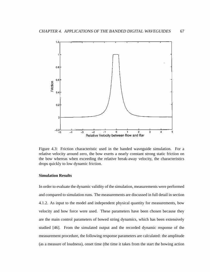
CHAPTER 4. APPLICATIONS OF THE BANDED DIGITAL WAVEGUIDES 67
Figure 4.3: Friction characteristic used in the banded waveguide simulation. For arelative velocity around zero, the bow exerts a nearly constant strong static friction onthe bow whereas when exceeding the relative break-away velocity, the characteristicsdrops quickly to low dynamic friction.
Simulation Results
In order to evaluate the dynamic validity of the simulation, measurements were performed
and compared to simulation runs. The measurements are discussed in full detail in section
4.1.2. As input to the model and independent physical quantity for measurements, bow
velocity and bow force were used. These parameters have been chosen because they
are the main control parameters of bowed string dynamics, which has been extensively
studied [46]. From the simulated output and the recorded dynamic response of the
measurement procedure, the following response parameters are calculated: the amplitude
(as a measure of loudness), onset time (the time it takes from the start the bowing action

CHAPTER 4. APPLICATIONS OF THE BANDED DIGITAL WAVEGUIDES 68
to reach a maximum amplitude self-sustained oscillation), fundamental pitch (lowest
dominant peak in measured spectrum) and spectral centroid (the center of gravity of
the spectrum as measure of spectral content). All these are descriptive of the dynamic
behavior.
Simulations using banded waveguides were performed in 12 steps between normal-
ized input parameters of velocity and force yielding 144 data points. At each point, the
amplitude, onset time, fundamental and spectral centroid were extracted from the data.
The simulations show qualitative similarity with the measured parameters (see sec-
tion 4.1.2). The output amplitude shows a clear positive correlation with velocity and
is largely independent of the force (figure 4.4) which mirrors experimental behavior
(Figures 4.8 and 4.9). A separation of regions of oscillations and non-oscillation can
also be seen in this figure. The onset time decreases with increasing force (Figure 4.5
is at a normalized input velocity of0.75) which is also seen in experiment (see Figure
4.16). However the surface plot reveals a more complicated dependency of the onset time
with force and velocity which goes beyond the measurements made. The fundamental
frequency is independent of both force and velocity in simulation and measurement. The
observed spectrum is harmonic in either case. The simulations show that the spectral
centroid is independent of both force and velocity, as found in the measurements (see
Figure 4.15). The details of the experiments will be discussed in the next section. In
addition to the experimental comparison, the model shows additional behavior that is
observed in qualitative performance and theoretically known for non-linear systems. For
instance it is possible to lock to various modes depending on the input parameters, just as
it is possible to lock to higher modes in performance.

CHAPTER 4. APPLICATIONS OF THE BANDED DIGITAL WAVEGUIDES 69
Figure 4.4: Amplitude as a function of input force and velocity in a bowed bar simulationusing the banded waveguide method.
4.1.2 Experimental Measurements
Now I will discuss experiments that have been performed to study the behavior of bowing
on rigid bars. This is the first time that such experiments have been performed and I
describe here the complete results.
The primary goal of the experiment was the measurement of parameters which are
of importance for musical performance when bowing bar percussion instruments. The
parameters in control of the performer are primarily bowing velocity and bowing force.
Parameters like angle, type of bow, amount of rosin were not considered in detail in
these experiments. The performance parameters of interest were assumed to be loudness,
temporal responsiveness, pitch, timbre and brightness. Other interesting parameters like

CHAPTER 4. APPLICATIONS OF THE BANDED DIGITAL WAVEGUIDES 70
Figure 4.5: Onset time as a function of input force in a bowed bar simulation using thebanded waveguide method.
ease of performance and “feel” of the bowing action were not investigated directly. From
the measured parameters the region of oscillation is derived, but effects like the ease of
locking to higher modes were not considered at all.
Loudness was measured by calculating the energy of the signal. Temporal respon-
siveness was measured as the time it took from starting the bowing action to reaching
a maximum amplitude self-sustained oscillation. This time will be referred to as onset
time. Pitch was measured by finding the fundamental in spectra taken from the measured
signals. Timbre and brightness was measured by calculating the spectral centroid of the
spectra of the measured signals.

CHAPTER 4. APPLICATIONS OF THE BANDED DIGITAL WAVEGUIDES 71
Two distinct measurement setups were used. First, a number of bars of different size,
shape and material were bowed by hand using a double bass bow. These measurements
were performed to get a qualitative result of most of the described quantities.
In order to get more quantitative and reproducible measurements, a bowing machine
was built and one bar was systematically studied for quantitative relationships between
input (bow) velocity and force to output amplitude, energy, fundamental frequency, spec-
tral content and onset time. These results will be described in section 4.1.2.
Measurements by Hand Bowing
Experimental Setup
For hand bowing, two different types of bars were used. One set of bars consisted of bars
taken from real musical instruments. These bars are undercut to tune the upper partials to
be close to harmonic. In this set, a bar representing the xylophone and marimba family
and bars for vibraphones were used. Xylophone and marimba bars are made of wood
(typically rosewood) whereas vibraphone bars are metal (typically aluminum).
The second set of bars consisted of wood and aluminum bars of uniform cross-section.
These have inharmonic partials. The measurement of bars of uniform thickness has two
purposes. For one it serves as comparison to the behavior measured for undercut bars.
Secondly the Euler-Bernoulli equation for constant cross-section and homogeneous ma-
terial is a linear fourth-order partial differential equation which lends itself to analytical
treatment, which is otherwise not easily possible.
A sketch of the typical shape of a bar can be found in figure 4.65. Table 4.1 shows
the dimensions of the measured bars and table 4.2 shows the position and size of the
5Figure 4.6 has been corrected compared to [61]. The positions of the cord holesx1r , x1l , x2r andx2l
were wrongly indicated.

CHAPTER 4. APPLICATIONS OF THE BANDED DIGITAL WAVEGUIDES 72
l w h l1 l2 h1 E ρ(cm) (cm) (cm) (cm) (cm) (cm) (GPa) (km/m3)
Uniform wood 38.1 4.05 1.95 N/A N/A N/A 10 640C#
4 wood 30.7 3.5 1.6 17.3 7.0 0.5 16 740Uniform 17.8 3.8 0.3 N/A N/A N/A 70 2710aluminumF#
4 aluminum 29. 3.9 1.36 11.95 5.3 0.6 70 2710F#
3 aluminum 36.4 5.1 1.36 16.4 9.3 0.5 70 2710
Table 4.1: Dimensions and material constants of measured bars
cord holes. The material constants (Young’s modulus and the mass density) were taken
from a standard reference (see Table 19.1 p. 625) [70] and were not measured for the
experimental bars.
Figure 4.6: Sketch of shape and dimensions of a bar.
The bar to be measured was suspended using two stiff cords under tension between
two vices. The microphone was placed underneath the middle of the bar. The typical
6The thickness of the vibraphone bars was misprinted as1.8 in [61] and has been corrected.

CHAPTER 4. APPLICATIONS OF THE BANDED DIGITAL WAVEGUIDES 73
x1r (cm) x1l (cm) x2r (cm) x2l (cm) d (cm)Uniform wood 3.9 3.9 3.9 3.9 0.7C#
4 wood 5.8 5.8 6. 5.6 0.5Uniform aluminuma 4. 4. 4. 4. N/AF#
4 aluminum 5.7 5.8 5.6 6.2 0.6F#
3 aluminum 7.3 7.4 7.5 6.8 0.6
Table 4.2: Positions and diameter of cord holes in barsaThe aluminum bar had no cord holes. Instead if was held in place by rubber bands on thin plastic rods
which were wrapped with felt at the given positions.
bowing point when bowing xylophone or vibraphone bars in a complete instrument is on
the narrow end, as this is the only side which can be conveniently reached with a bow
by the performer. Hence our measurements concentrate on bowing positions on the end
of the bar. In some bowing strokes, especially when high bowing forces are applied, the
oscillation of the mass spring system of the cords and the bar had to be damped by placing
one hand on one of the cords and pulling down. The typical setup is depicted in figure
4.7. A rosined double bass bow was used for all hand bow measurements.
Measurement results
First, the response of the measured bars to impulsive excitation was measured using both
a force hammer and a hard plastic glockenspiel mallet. Table 4.3 shows the frequencies
of the dominant partials of each test bar along with the theoretical values for uniform bars
as well as the usual tuning frequencies for undercut bars. As can be seen, the uniform
aluminum bar is very close to the values predicted by the Euler-Bernoulli theory. The
uniform wooden bar deviates substantially from the theoretical values, for two likely
reasons. One is that the bar is not perfectly uniform due to the holes drilled3.95cmfrom
both ends with a diameter of0.75 cm. Second, the thickness is comparable to the width

CHAPTER 4. APPLICATIONS OF THE BANDED DIGITAL WAVEGUIDES 74
Figure 4.7: Experimental setup for hand bowing measurements of bars.
of the bar, in which case the application of the Timoshenko theory is more appropriate,
which lowers the frequency of the upper partials [70].
The bowed bar exhibits a harmonic spectrum, though often weaker partials at the
possibly inharmonic eigenfrequencies can be seen. This behavior can also be seen when
bowing at positions other than one of the free ends. Bowing at the side is easily possible
only with sufficient distance to the suspension holes. When bowing in the middle, the
fundamental of the bar can also be excited. For the F#3 vibraphone bar bowing in the
middle will often lock to the second eigenfrequency of the bar, which lies two octaves
above its fundamental eigenfrequency. This tendency to lock to the higher mode can
usually only be overcome with increasing friction by tilting the bow or by other means.

CHAPTER 4. APPLICATIONS OF THE BANDED DIGITAL WAVEGUIDES 75
Wooden Aluminum Usual C#4 F#3 F#
4n Theory (uniform) (uniform) tuning xylo vibra vibraf1 693.9 487. 280.6 187.3 373.62 2.756 2.572 2.756 4. 3.932 3.984 3.9973 5.404 4.644 5.423 10. 9.538 10.668 9.4694 8.933 6.984 8.988 16.688 17.979 15.5665 13.346 9.723 13.448 24.566 23.679 20.8636 18.6408 18.680 31.147 33.642 29.440
Table 4.3: Spectral frequencies of dominant partials of measured bars and theoreticalvalues given asfn : f1. The left side of the table contains the theoretical prediction foruniform bars and the actually measured ratios of the two measured bars. The right sidecontains the usual tuning and the measured ratio for tuned bars. The first row containsthe actual fundamental frequencyf1 of the bars.
Another possible way of excitation is to contact the top surface of the bar. By bowing
with little bowing force a proper regime of oscillation can be excited.
Using hand bowing, a qualitative relationship between bowing velocity and amplitude
as well as between bowing force and amplitude was investigated. It should be noted that
constancy of velocity and force within each measurement as well as across measurements
(when applicable) were not possible as they are highly dependent on the subjective per-
ception and the skill of the performer. As will be seen in the quantitative measurements
using a bowing machine, the lack of constancy of bowing force is likely not a problem as
the amplitude appears to be independent of the bowing force.
Figures 4.8 and 4.9 show the time domain envelopes of bowing strokes with increas-
ing velocity and increasing force. From the length of the bow and the stroke time,
which can be retrieved from the time-domain plot, an average input velocity can be
deduced. Setting this velocity in relationship to the amplitude of the signal shows an
approximately linear increase of amplitude with increasing velocity. Force was held
nearly constant in the velocity measurement. The force measurement shows no clear

CHAPTER 4. APPLICATIONS OF THE BANDED DIGITAL WAVEGUIDES 76
Figure 4.8: Time-domain amplitude envelope of hand strokes with increasing velocityand force held approximately constant.
influence on the amplitude. This finding was later validated by the bowing machine
measurements. The time-domain shapes of the force-amplitude relation also hint at a
decrease of onset time with increasing force. This result was also quantified using bowing
machine measurements, as described in the next section.
Measurements using the Bowing Machine
Experimental Setup
The F#3 aluminum vibraphone bar under investigation (see table 4.1) was suspended in a
rigid bar holder. The holder has two effects. First it removes the cord modes or other
movements which are not of interest while keeping the important degrees of freedom.

CHAPTER 4. APPLICATIONS OF THE BANDED DIGITAL WAVEGUIDES 77
Figure 4.9: Time-domain amplitude envelope of hand strokes with increasing force andvelocity held approximately constant.
Second, it allows very high bowing forces to be applied by the bowing machine. As
shown in Figure 4.10 angled screws were screwed into a wooden base at the positions of
the cord holes of the bar. Rubber tips were placed between the metallic holder and the
bar to minimize the friction noise and keep a flexible interface. The wooden base was
shaped to allow bowing at the narrow side and at the wide side at positions between the
suspension holes. In the bowing machine measurement, the bar was pulled towards the
bowing machine (which will be described in the next section), by means of a cord which
was tied to a hook on one narrow side of the bar holder. When the applied force was
measured, the cord was replaced by a spring scale with a scale range of0 to 2000grams.

CHAPTER 4. APPLICATIONS OF THE BANDED DIGITAL WAVEGUIDES 78
Figure 4.10: Experimental setup for bowing machine measurements of bars.
The microphone position for these measurements was above the middle of the bar as the
bar holder didn’t leave enough space underneath the bar.
Bowing Machine
The bowing machine consisted of a standard variable speed power drill, a cylindrical
drum of hard rubber with a2.6 cm radius and width of3.75 cm around which a band
of horse hair was wound and glued together at the open ends using super-glue to form a
loop. The typical loop width and thickness was comparable to the width of the double
bass bow. The horse hair was then rosined. In order to calibrate bowing speed, a bicycle
speedometer was added to the drill. The magnet was placed on the rotating part and

CHAPTER 4. APPLICATIONS OF THE BANDED DIGITAL WAVEGUIDES 79
the pickup sensor was glued to the non-rotating casing of the drill reaching over the
magnet. In measurement, the bowing drill was held in place by a vice and the bar was
pulled against it. The noise of the drill was damped from the recording by placing sound-
absorbing foam between the drill and the microphone. Also the microphone position was
generally facing away from the drill and towards the primary sound radiation direction
of the bar, enhancing the signal to noise ratio. The microphone position was adjusted to
maximize the signal from the bar while avoiding saturation.
Measurement procedure
Figure 4.11: Bowing machine measurement series 1: Measured input parameters: Forceand velocity.
Two series of measurements were performed using the bowing machine described
in the previous section. Before each series the bowing drum had to be rehaired and

CHAPTER 4. APPLICATIONS OF THE BANDED DIGITAL WAVEGUIDES 80
Figure 4.12: Bowing machine measurement series 2: Measured input parameters: Forceand velocity.
new rosin was applied. Hence it should be noted that direct quantitative comparisons
between these two series are not easily possible. The reason for the need to rehair the
bowing machine stems from the fact that the high force measurements at the end of each
series resulted in breaking of the hair loop and hence rendered the loop useless for more
measurements. There is another reason why the measurements should not be compared
between measurement series. The microphone was moved and recalibrated between the
series and hence the attenuation of output levels between series should be expected to be
different.
The unevenness and change of stiffness of the hair loop at the glue joint yielded an
overlap of impulsive excitations over the total bowing excitation. This effect can be ex-
pected to influence some of the behavior measured. The impulses overlaying the overall
CHAPTER 4. APPLICATIONS OF THE BANDED DIGITAL WAVEGUIDES 81
sound were used as an independent measure of velocity because of the occurrence of
one impulse per revolution. Later this measurement was correlated with the independent
velocity measurement using a speedometer to get an error estimate.
The first series consisted of nine runs starting at a particular bowing speed in gradually
increasing forces between0 and14 Newtons (or0 and2000grams spring scale readings
with a relative force contribution of√
2 due to an angle of45degrees). Forces were taken
at the following spring scale readings if oscillations occurred:125, 250, 500, 1000, 1250,
1500, 1750and2000grams. In this measurement series, the oscillation was not damped
out and restarted at each measurement point, but the force was steadily increased with the
bowing machine continuously in contact. The setting of the drill speed was not adjusted,
which resulted in a decrease of the actual bowing speed due to the reduced drill speed
from the increased force load. All measurement points can be seen in figure 4.11. As
can be seen, the velocity of each run decreases as a function of input force. The velocity
was derived from the recording as described before. The last run (run 9) didn’t result in
oscillation and hence indicates points lying beyond the upper velocity limit.
These measurements were aimed towards finding the regions of oscillation as a func-
tion of velocity and force. In addition relative energy as a function of velocity and force
was calculated from the recorded sounds and the change in spectral content was charac-
terized using the spectral centroid, which is the center of gravity of the spectrum. The
spectral centroid correlates roughly with brightness. Finally, the fundamental frequency
of the recorded sounds was also measured. The results will be discussed in subsequent
sections.
The second series consisted of three runs again starting at a particular bowing speed.
This time the oscillation was damped out after recording for each measurement point and,
using the attached speedometer, the input velocity was adjusted in the attempt to keep

CHAPTER 4. APPLICATIONS OF THE BANDED DIGITAL WAVEGUIDES 82
Figure 4.13: Bowing machine measurement series 1: Recorded radiation energy as afunction of bowing velocity.
the actual bowing speed roughly constant. If a measurement point yielded oscillation
the recording was taken long enough to measure the full oscillation build-up until the
maximum and a significant part of the steady state oscillation. Hence in addition to all
the measures derived from series 1, the onset transient time until maximum oscillation
was reached was measured in this series. The force range was extended for the first two
runs of this series to a maximum force of about20 Newtons (or a spring scale reading of
2000grams at0 degrees angle).
All measurement points of this series can be found in figure 4.12. The velocities
were measured both using the measure of the speedometer and from the recording. A
correlation between the two independently measured velocity values shows the average
error to be2.21 cm/s (or 1.2%) with a standard deviation of2.06 cm/s (or 1.1%). As

CHAPTER 4. APPLICATIONS OF THE BANDED DIGITAL WAVEGUIDES 83
can be seen, the error is very low. This has to do with the high number of revolutions
measured in both cases yielding a good resolution.
Results of bowing machine measurements
Region of oscillation
Figure 4.14: Bowing machine measurement series 2: Recorded radiation energy as afunction of bowing force.
As can be clearly seen from figure 4.11 the minimum bowing force increases as a
function of velocity. A maximum bowing force could only be found for the first two runs
of series 1, which are at velocities below50 cm/s. At higher bowing speeds an upper
force limit could not be found within the measurement range. The minimum speed at
which steady oscillation was found was23.83 cm/s with a force of13.87 N. It should

CHAPTER 4. APPLICATIONS OF THE BANDED DIGITAL WAVEGUIDES 84
Figure 4.15: Bowing machine measurement series 1: Spectral centroid as a function ofbowing force. Only measurement point with a clear steady-state oscillation are shown.
be noted that using the undamped measurement approach of series 1, very low velocities
can be achieved even for high forces (as can be seen from run 3 in figure 4.11. This point
is the highest measured force point in this run). The maximum bowing speed from series
one is found to be above203.72cm/sand below261.14cm/s.
Energy and power, spectral content, fundamental frequency and onset times
Both measurement series show that the energy of the fully developed steady state oscil-
lation increases as a function of velocity and the relationship seems to be approximately
linear (the measurements of the first series can be seen in figures 4.13). Taking this linear
velocity dependency into account, the energy radiation seems to be independent of the
input bowing force (this effect can be seen more clearly in series two, where the force-

CHAPTER 4. APPLICATIONS OF THE BANDED DIGITAL WAVEGUIDES 85
Figure 4.16: Bowing machine measurement series 2: Onset time as a function of bowingforce.
energy relationship as depicted in figure 4.14 correlates closely with the force-velocity
relationship as depicted in figure 4.12).
The spectral centroid of series 1 seems uncorrelated with the input force and velocity.
No clear upward trend was observed with increasing force (see figure 4.15) in contrast to
known behavior of the bowed string. Series 2 verifies this result.
The measurements of the fundamental frequency as a function of velocity and force
result in minor fluctuations without a clear trend. In series 1, the mean frequency was
186.67Hzwith a standard deviation of0.26Hz (33 data points) and in series 2, the mean
frequency was186.73 Hz with a standard deviation of0.27 Hz (25 data points). The
measurements as a function of velocity seem to indicate a trend towards flattening with
increasing velocity, whereas there is no trend observable in dependency of force. In any

CHAPTER 4. APPLICATIONS OF THE BANDED DIGITAL WAVEGUIDES 86
Figure 4.17: Bowing machine measurement series 2: Onset time as a function of bowingvelocity.
case, the effect is very small (less than10cents) even over the full range. High velocities
should be difficult to achieve by hand-bowing and hence within the usual bowing domain,
the dependency of the fundamental on the bowing parameters is negligible.
Onset time as a function of velocity and force was measured in series 2 only. As
was already noted from the time-domain shapes of hand-bowed measurements, there is
a clear decrease of the onset times with increasing bowing force (see figure 4.16). The
onset time appears uncorrelated with the input bowing velocity (see figure 4.17).
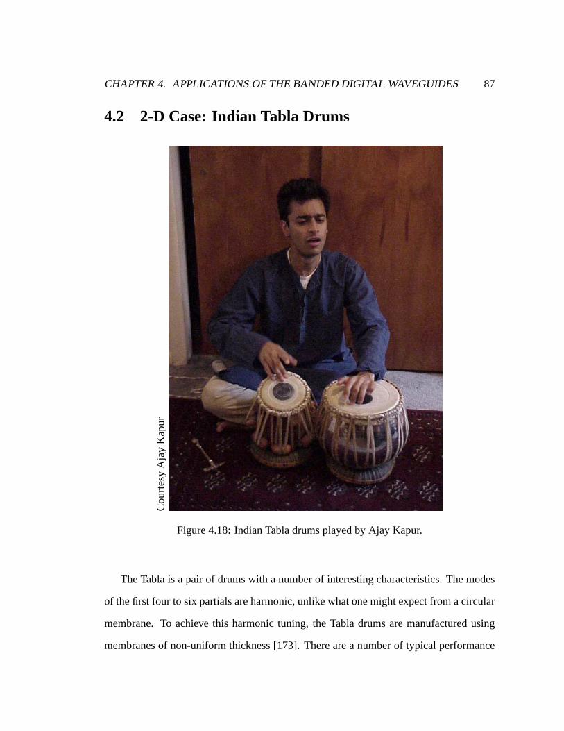
CHAPTER 4. APPLICATIONS OF THE BANDED DIGITAL WAVEGUIDES 87
4.2 2-D Case: Indian Tabla Drums
Cou
rtes
yA
jay
Kap
ur
Figure 4.18: Indian Tabla drums played by Ajay Kapur.
The Tabla is a pair of drums with a number of interesting characteristics. The modes
of the first four to six partials are harmonic, unlike what one might expect from a circular
membrane. To achieve this harmonic tuning, the Tabla drums are manufactured using
membranes of non-uniform thickness [173]. There are a number of typical performance

CHAPTER 4. APPLICATIONS OF THE BANDED DIGITAL WAVEGUIDES 88
strokes to Tablas. One interesting stroke is a modulating form of the “Ga” stroke, which
is performed on the larger, right drum, called “bayan.” The palm of the hand resides
on the drum. After the drum has been excited with a quick impact with the finger-
tips, the player pushes her palm down and towards the center of the drum and hence
achieves a characteristic upward pitch-bending sound [173]. Figure 4.18 shows Ajay
Kapur performing this stroke. The small drum is called dahina.
Using propagation modeling for this example highlights a number of issues. First, a
membrane of a Tabla is essentially a two-dimensional structure, and we no longer have
the simple direct interpretation of a banded waveguide as was possible for the bar. We
do know, however, that the modes correspond to closed wavetrains. To remove the men-
tioned ambiguity, we need additional information beyond the modal frequencies. One
possibility would be to try to derive this information from measured impulse responses.
Alternatively one can try to derive an analytical solution for the propagation of waves.
The drum head of the Tabla is non-uniform so analytical solutions of this sort are hard.
Also, modal frequencies which are usually separate are tuned to be aligned with each
other. This can be seen in Figure 4.19. Distinct modal patterns are tuned to be harmonic.
These modal patterns may indeed contain the information necessary to derive wave-
train closure paths. Circular modes are radially symmetric, hence the wavetrain closure
path has to go from the boundary through the center and back. Diagonal modal lines,
however, don’t follow that simplified one-dimensional interpretation.
In our model we chose to simply ignore the difficulties and approximate the propa-
gation. This could be interpreted as disregarding the multiplicity of eigen-modes or as
disregarding modal shapes with diagonal modal lines. However, it leaves us with a simple
one-dimensional model of the Tabla.

CHAPTER 4. APPLICATIONS OF THE BANDED DIGITAL WAVEGUIDES 89
Figure 4.19: The nine nodal patterns of the Tabla tuned to harmonic modes (after Rossing[173]).
Bayan Dahinan measured simulated measured simulated2 2.00 2.02 2.89 2.873 3.01 3.03 4.95 5.014 4.01 4.05 6.99 6.735 4.69 4.72 8.01 8.006 5.63 5.65 9.02 8.70
Table 4.4: Spectral frequencies of dominant partials of measured and simulated Tablasgiven asfn : f1.
In this case, the pitch-bending technique directly corresponds to shortening the phys-
ical path of waves traveling on the membrane, which can be directly implemented in a
propagation style simulation.
This is not a direct geometric correspondence, but rather a resemblance which is
modeled. Whether or not a precise geometric interpretation exists remains open.

CHAPTER 4. APPLICATIONS OF THE BANDED DIGITAL WAVEGUIDES 90
The results of modal comparison between real drums and propagation simulations can
be found in Table 4.4. The strokes performed are open membrane strokes in the center
on both the bayan and the dahina. This was in turn modeled as impulsive excitation.
Time
Fre
quen
cy
0.1 0.15 0.2 0.25 0.3 0.35 0.4 0.45 0.5 0.55 0.60
200
400
600
800
1000
1200
(a) Recorded
Time
Fre
quen
cy
0 0.1 0.2 0.3 0.4 0.50
200
400
600
800
1000
1200
(b) Simulated
Figure 4.20: Spectrogram showing the upward bending of a modulatedGa stroke. Thefundamental bends from 136 to 162 Hz (measured) and 134 to 171 Hz (simulated).
The results for the more complicated pitch-bending strokes can be seen in Figure 4.20.
The simulation shows good resemblance and sound comparable to the recorded stroke. It
should be noted that the simulation method is robust to the pitch-bending manipulation.
In fact, much more extreme bends than the one depicted here are possible. High pitched
large-scale bends on our propagational model perceptually closely resemble water-drop
sounds, suggesting a much wider range of interesting application for behaviors of this
type.
Hence, despite the forced reduction in dimensionality and loss of geometric interpre-
tation, the simulation achieves good results for complex interactions.

CHAPTER 4. APPLICATIONS OF THE BANDED DIGITAL WAVEGUIDES 91
4.2.1 Periodic Orbit on Circular Domain
In order to recover a more full notion of spatial location, the topology of periodic orbits
on the domain have to be constructed.
The circular domain is an often studied canonical example [104, 25]. It can be seen
that in fact the circular domain is very similar to the rectangular domain discussed in
section 3.9.2. Both examples have two independent spatial dimensions and are integrable
systems7. Hence EBK quantization via a resonant torus applies and a canonical transform
from domain variables to torus dimensions can be found.
Figure 4.21: Radial and angular variables on a circular domain and their connectedturning properties.
The difference between dimensions in the rectangular domain and the circular domain
is the independent variables of radiusr and angular positionφ already are topologically
connected (as illustrated in Figure 4.21). For the case of the radius, this can be seen
7A system is integrable if it admits the maximum number of integrals of motion (for a rigorous definitionsee [25, p. 60]).

CHAPTER 4. APPLICATIONS OF THE BANDED DIGITAL WAVEGUIDES 92
following a diagonal trajectory through the origin of the circle. Towards the center the
radial variable decreases until atr = 0 the radial variable “turns” and then increases until
the boundary is reached. Also the angular variable repeats itself after2π. Whereas the
position of the radial turning point has a defined position on the domain (namely the
center), the reference of the circular repetition is a matter of definition and the point
indicated in Figure 4.21 is just a possibility. Hence looking at the circular domain the
set of paths with inward and outward radial motions and connecting these two sets at the
boundary yields the EBK resonant torus of Figure 3.9.
As mentioned in section 3.9.2 the class of all turning points inside the domain of a
family of rays is called caustics. In this case, these are the radial turning points, which
form a circle inside the domain8 (see Figure 4.22).
In the case of the rectangular domain, the family of rays with equal winding properties
on the torus were defined by the ratiox1 : x2 and now this property is defined by the ratio
r : φ. Hence all rays with the same reflection angle at the boundary belong to a family of
rays with the same resonant properties.
Any ray with a non-zero radial propagation component (see Figure 4.22(a)) hence
alternates between reflecting at the boundary and touching the caustic and hence in the
quantization condition (3.24), the Maslov indexµ, counting caustic turning points, and
the number of boundaries reached,b, are both equal and1 or more.
The special case of a purely angular propagation component neither reaches a bound-
ary nor turns radial components (see Figure 4.22(b)) and hence bothµ andb are zero and
the path length is simply the circumference of that circular path2πa0 (compare [104, eq.
(23)]):
8The general theory of caustic phenomena is a rich and complex field and will not be discussed fullyhere. See [110] for a mathematical treatment of caustic phenomena.
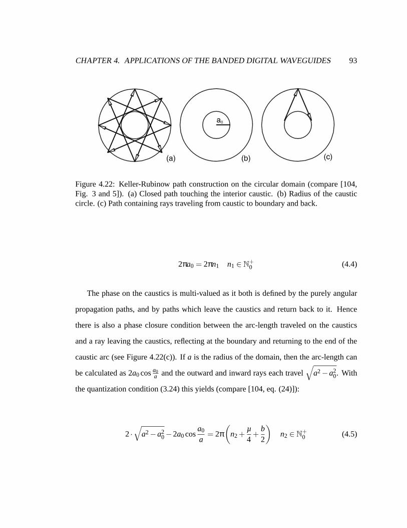
CHAPTER 4. APPLICATIONS OF THE BANDED DIGITAL WAVEGUIDES 93
Figure 4.22: Keller-Rubinow path construction on the circular domain (compare [104,Fig. 3 and 5]). (a) Closed path touching the interior caustic. (b) Radius of the causticcircle. (c) Path containing rays traveling from caustic to boundary and back.
2πa0 = 2πn1 n1 ∈ N+0 (4.4)
The phase on the caustics is multi-valued as it both is defined by the purely angular
propagation paths, and by paths which leave the caustics and return back to it. Hence
there is also a phase closure condition between the arc-length traveled on the caustics
and a ray leaving the caustics, reflecting at the boundary and returning to the end of the
caustic arc (see Figure 4.22(c)). Ifa is the radius of the domain, then the arc-length can
be calculated as2a0cosa0a and the outward and inward rays each travel
√a2−a2
0. With
the quantization condition (3.24) this yields (compare [104, eq. (24)]):
2·√
a2−a20−2a0cos
a0
a= 2π
(n2 +
µ4
+b2
)n2 ∈ N+
0 (4.5)

CHAPTER 4. APPLICATIONS OF THE BANDED DIGITAL WAVEGUIDES 94
Then the multi-valuedness is removed by eliminatinga0 from equations (4.4) and
(4.5):
2·√
a2−n21−2n1cos
n1
a= 2π
(n2 +
µ4
+b2
)n1,n2 ∈ N+
0 (4.6)
This equation corresponds to [25, p. 88, eq. (2.153)]. The quantization numbers
n1 andn2 correspond to the nodal numbers depicted in Figure 4.19 and established the
connection between ray paths and spatial modes.
In order to follow the derivation simplifying assumptions are made and hence the
topological construction is an approximate one.
4.3 3-D Case I: Wine Glasses and Glass Harmonicas
Drinking glasses, in particular wine glasses, can be made to ring in many different ways.
They can be excited by impact, by rubbing the top rim with a wet finger, or by radially
bowing with a violin bow. While impact can easily be simulated using modal models,
rubbing and bowing cannot. Geometrically, a wine glass is a three-dimensional object
and disturbances travel along the object in all dimensions. The object is symmetrical,
however, and the dominant modes are essentially two-dimensional [173]. One is left with
bending modes along the cylindrical axis, which can be excited by rubbing, plucking
or bowing, but most of the energy really goes into flexural modes of the circumference
of the glass. This is a closed path — essentially a bar being bent into a circular shape,
closing onto itself. Hence the path is quasi one-dimensional. The path traced along the
wine glass can be seen in Figure 4.24.

CHAPTER 4. APPLICATIONS OF THE BANDED DIGITAL WAVEGUIDES 95
Cou
rtes
yE
dG
aida
Figure 4.23: Benjamin Franklin’s glass harmonica, which he called “armonica”, as seenin the Franklin Institute Science Museum in Philadelphia.
From the distance to be traveled along the rim, the circumference of a circlel = 2πr,
and the wave velocity from equation (4.2) we can derive the actual frequency and its
connection to traveling length [173], which completely determines the wavetrain closure
to be modeled:
1ω
=lv
=2πr√aω
ω =a∗
r2
(4.7)

CHAPTER 4. APPLICATIONS OF THE BANDED DIGITAL WAVEGUIDES 96
(a) 3-D model view (b) Top view
Figure 4.24: The wavetrain closure on the rim of a wine glass and corresponding flexuralwaves as seen from the top (after Rossing [173]).
Due to the circularity of the path, the banded waveguide system makes no reference
to the actual position on the rim. In practice, however, the point of interaction provides
this reference. If the glass is struck, the point of excitation is defined along the circle. The
same is true for bowing, which usually happens at one point radially to the rim. Rubbing
the rim is a peculiar case because the point of interaction is moving slowly along the
path. In our model, we make no distinction between rubbing and bowing as the rubbing
is a very slow motion compared to the wave traveling on the path, and hence treating the
rubbing interaction as stationary does not significantly alter the non-linear behavior. The
effect of the slowly shifting interaction point is measurable, though not audible as it is
too slow [173].

CHAPTER 4. APPLICATIONS OF THE BANDED DIGITAL WAVEGUIDES 97
Struck Rubbed Bowedn measured sim. measured measured sim.2 2.32 2.31 2.00 2.00 2.003 4.25 4.20 3.00 2.99 3.004 6.63 6.69 4.00 4.005 9.38 8.81 5.00 5.00 5.00
Table 4.5: Spectral frequencies of dominant partials of measured and simulated struck,rubbed and bowed wine glass given asfn : f1.
Results of measurements and simulations are presented in Table 4.5. The struck
excitation was a quick sharp strike with a finger nail against the glass, which was modeled
using a simple impulse. Bowing on the real glass was performed using a rosined violin
bow. The rubbing was performed with a wet finger. With the violin bow it is possible
to excite the second harmonic as the fundamental frequency of the bowing response.
The same result can also easily be achieved using the simulation model. The simulation
model captures both the harmonic spectra as well as a other non-linear effects of the real
interaction. We did not model a rubbed interaction separately as we assume it follows in
principle the same mechanism as bowing [69]9.
4.4 3-D Case II: Tibetan Singing Bowl
The Tibetan singing bowl are geometrically close to spherical segments. A discretized
mesh version of the bowl can be seen in Figure 4.25). In typical performance, the bowl is
rubbed with a wooden stick wrapped in a thin sheet of leather along it’s rim. Depending
on the rubbing velocity and initial state of the bow (i.e. certain modes may be already
9After the completion of the thesis I became aware of work by Serafin and co-workers whoindependently implemented a Tibetan bowl using banded waveguides — the object of study of the nextsection — in the context of demonstrating a novel rubbing board controller. The paper [221] does not givetechnical details, but the sounds presented at the conference were impressive.

CHAPTER 4. APPLICATIONS OF THE BANDED DIGITAL WAVEGUIDES 98
Cou
rtes
yJa
mes
F.O
’Brie
n
Figure 4.25: Mesh of simulated bowl.
ringing), various frequencies can be made to oscillate. Behavior is comparable to rubbing
or bowing a wine glass in terms of dynamic envelope, mode locking, mode duplication
and related phenomenon as a result of the non-linear interaction of the stick-slip-based
rubbing.
Cou
rtes
yJa
mes
F.O
’Brie
n
Figure 4.26: Simulated mode shapes of the bowl.
If struck, the bowl will show a modal response of circular-symmetric form. The first
few modal shapes are depicted in Figure 4.26 with exaggerated amplitudes. These shapes
will oscillate around the circular rest position comparable to circular flexing motion of
the wine glass depicted in Figure 4.24. The circularly repeating pattern is depicted in
Figure 4.27. This picture also shows non-circular modes, which tend not to be excited by
the circular rubbing motion.

CHAPTER 4. APPLICATIONS OF THE BANDED DIGITAL WAVEGUIDES 99
Figure 4.27: Path of circular mode on bowl (used with permission from (Cook 2002).)
The measured spectra of the struck bowl can be seen in Figure 4.28 for various impact
positions. As can be seen, there are a number of higher modes which lie close together
yielding audible beating. The beating can be seen more clearly in Figure 4.29.
4.4.1 Beating Banded Waveguides
While beating modes in physically separate structures have been studied in the case of
coupled piano strings [8, 9, 6] and plucked strings with sympathetic coupling [99], the
modeling of beating within the banded waveguide remains unexplored.
The beating modes combined with the very weak damping poses the main challenge
for modeling the dynamics using banded waveguides (as depicted in Figure 3.3.)
For two neighboring banded wavepaths whose center frequencies get close, the re-
spective frequency-bands start to overlap strongly. This means that energy will con-
tribute to traveling waves in both bands simultaneously. To guarantee stability within
the frequency region the sum gain of both waveguides cannot exceed unity as both are
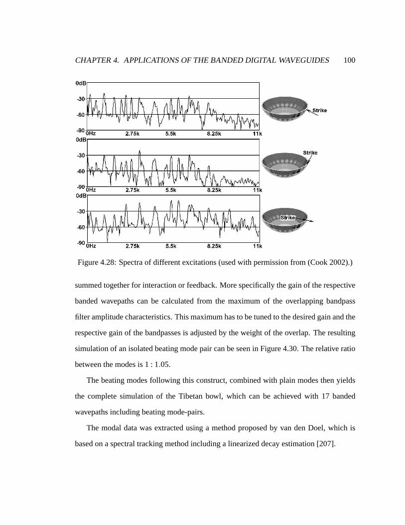
CHAPTER 4. APPLICATIONS OF THE BANDED DIGITAL WAVEGUIDES 100
Figure 4.28: Spectra of different excitations (used with permission from (Cook 2002).)
summed together for interaction or feedback. More specifically the gain of the respective
banded wavepaths can be calculated from the maximum of the overlapping bandpass
filter amplitude characteristics. This maximum has to be tuned to the desired gain and the
respective gain of the bandpasses is adjusted by the weight of the overlap. The resulting
simulation of an isolated beating mode pair can be seen in Figure 4.30. The relative ratio
between the modes is1 : 1.05.
The beating modes following this construct, combined with plain modes then yields
the complete simulation of the Tibetan bowl, which can be achieved with17 banded
wavepaths including beating mode-pairs.
The modal data was extracted using a method proposed by van den Doel, which is
based on a spectral tracking method including a linearized decay estimation [207].

CHAPTER 4. APPLICATIONS OF THE BANDED DIGITAL WAVEGUIDES 101
Time (s)
Fre
quen
cy (
Hz)
0 0.5 1 1.53000
3500
4000
4500
5000
5500
6000
Figure 4.29: Beating upper partials in spectrogram of a recorded Tibetan bowl.
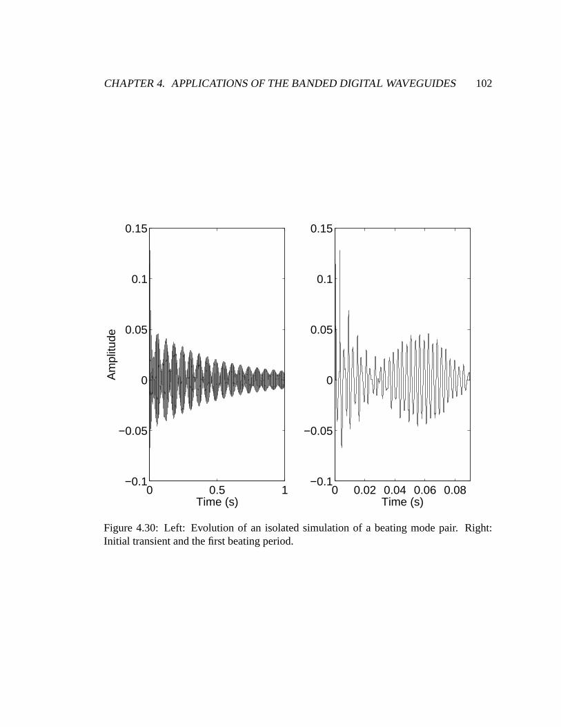
CHAPTER 4. APPLICATIONS OF THE BANDED DIGITAL WAVEGUIDES 102
0 0.5 1−0.1
−0.05
0
0.05
0.1
0.15
Time (s)
Am
plitu
de
0 0.02 0.04 0.06 0.08−0.1
−0.05
0
0.05
0.1
0.15
Time (s)
Figure 4.30: Left: Evolution of an isolated simulation of a beating mode pair. Right:Initial transient and the first beating period.

Chapter 5
Comparison with Alternative Methods
Is it progress if a cannibal uses knife and fork? – Stanislaw J. Lec1
One of the symptoms of an approaching nervous breakdown is the belief that
one’s work is terribly important. – Bertrand Russell2
This book fills a much-needed gap. – Moses Hadas3
5.1 Modal Synthesis
Modal synthesis [208] and propagation modeling are conceptually very close. The main
difference between the two is that the latter maintains the relative phase responses of
the modes and approximates the phase response between modes. In terms of physical
interpretation, modal synthesis is blind to the mechanism that gives rise to the resonance,
whereas propagation synthesis is not. Modal synthesis is inflexible with regards to in-
teraction and observation points, whereas propagation modeling allows for constructions
1In “Unkempt Thoughts,” Funk & Wagnalls, p. 78 (1962)2In “The Conquest of Happiness,” chap 5. according to [147, p. 551, q. 10]3Attributed by J. E H. Shaw, “Some Quotable Quotes for Statistics,” 2001, available athttp://www.
warwick.ac.uk/statsdept/Staff/JEHS/data/jehsquot.pdf
103

CHAPTER 5. COMPARISON WITH ALTERNATIVE METHODS 104
which give a physically meaningful interpretation to interaction points and observation
points, at least in the one-dimensional case. In higher-dimensional cases, the spatial
interpretation is difficult and symmetries have to be exploited. Computationally, both
methods share the same complexity. Banded waveguides model the same number of
modes but with the addition of one inexpensive delay-line per mode.
5.2 Waveguide Synthesis
Waveguide synthesis [187] can be seen as a special case of propagation modeling in
which the group delay of all frequencies is constant and hence band-limiting and sep-
aration of modes become unnecessary. Both methods share an obvious physical inter-
pretation and justification. For both, results of linear transmission line and digital filter
theory can be utilized. Two and three-dimensional waveguide meshes differ from propa-
gation modeling, as waveguide meshes maintain the physical space, whereas propagation
models reduce dimensionality to wavetrain path analogues. It should be noted, however,
that waveguide meshes are not computationally efficient as the commutability is lost.
Propagation modeling maintains efficiency even for higher-dimensional simulations. An-
other way of comparing traditional waveguide models and propagation models is by the
way they handle dispersion. In waveguide models dispersion effects are lumped together
and modeled in one all-pass filter [187] whereas in propagation models the dispersion
is distributed. Propagation models hence more closely model the physical qualities at
local points with regards to dispersion. This difference is relevant as waveguide models
become inefficient with increasing dispersion as the filter order to implement appropriate
lumped all-pass filters becomes high.

CHAPTER 5. COMPARISON WITH ALTERNATIVE METHODS 105
5.3 All-pass Chains and Frequency Warping
An alternative approach to the banded waveguide structure to model non-constant wave-
propagation is to replace the unit delay with all-pass filters that model the non-constant
propagation characteristics. In [60] we called this structure “generalized waveguide”
although in this thesis I referred to banded waveguides as “generalized digital wave-
guides” (see section 3.6). Here I will rather call the first “all-pass waveguides” to note
the distinction.
The all-pass waveguide is the spatial discretization of the propagation equation (see
3.14). As can be seen, the phase velocity depends on the frequency. Starting from the
picture of the usual waveguide, the unit delays are replaced by frequency dependent
delays as symbolically depicted in figure 5.1.R is the appropriate reflection-function
at the boundary.
Figure 5.1: All-pass-chain or warped frequency waveguide.
If losses are modeled separately, the frequency dependent delays are all-pass filters
with an appropriately modeled phase delay response. This has strong connections to and
is strongly motivated by work on modeling the stiffness of strings starting from a mixed
bar/string-equation using all-passes [94, 145, 213, 169].
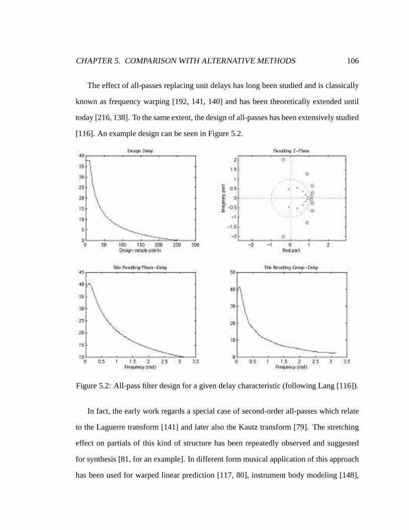
CHAPTER 5. COMPARISON WITH ALTERNATIVE METHODS 106
The effect of all-passes replacing unit delays has long been studied and is classically
known as frequency warping [192, 141, 140] and has been theoretically extended until
today [216, 138]. To the same extent, the design of all-passes has been extensively studied
[116]. An example design can be seen in Figure 5.2.
Figure 5.2: All-pass filter design for a given delay characteristic (following Lang [116]).
In fact, the early work regards a special case of second-order all-passes which relate
to the Laguerre transform [141] and later also the Kautz transform [79]. The stretching
effect on partials of this kind of structure has been repeatedly observed and suggested
for synthesis [81, for an example]. In different form musical application of this approach
has been used for warped linear prediction [117, 80], instrument body modeling [148],

CHAPTER 5. COMPARISON WITH ALTERNATIVE METHODS 107
reduction of dispersion errors in waveguide meshes [176], audio effects [66, 65] and
warping to perceptual scales [189]. Otherwise it’s been studied in modeling room impulse
responses [107], the approximation of delay systems [119, 118] and system identification
[7, 67], filter design [120], and image compression [41]. Cascaded all-passes, possibly
mixed with delays have long been used in reverberation algorithms [49, for example].
In the case of all-pass waveguides, depending on the order of the all-passes used,
good approximation to the propagation characteristics can be achieved, this approach
shows poor performance. The number of all-passes needed depends on the fundamen-
tal frequency of the instrument. It was found that for the same spatial and temporal
sampling, 10th order all-pass chains require more computation than an implicit finite
difference method implementation (after [35]). This performance comparison matches
the counted number of floating-point multiplications and additions as found in the all-
passes and the band-diagonal solver used in the finite difference implementation. While
this model preserves spatial sampling and hence would allow for non-linear spatially
localized interactions, it is neither useful for musical performance nor advisable for
acoustical modeling purposes, because finite differencing also model local coupling terms
at the same complexity.
In fact, it should be noted that an interesting conceptual difference between all-pass
waveguides and banded waveguides is the spatial sampling. All-pass waveguides use
uniform spatial sampling with each all-pass unit corresponding to a spatial unit. As
was discussed in section 3.7 banded waveguide have multi-scale spatial sampling. This
difference provides the crucial performance improvement.

CHAPTER 5. COMPARISON WITH ALTERNATIVE METHODS 108
5.4 Modal Decomposition & Green’s Function
Propagation modeling is a simplification and possibly an approximation to full modal
decomposition or Green’s function modeling. By full modal decomposition modeling,
we mean the modal description of the system which keeps both the modal frequencies
(as modal synthesis does) and modal shapes (corresponding to eigenvectors of the sys-
tem) [134]. In a propagation perspective, eigenvectors can intuitively be interpreted as
capturing the details of the wave-path which gives rise to the closed wavetrain. Propa-
gation modeling keeps only the total roundtrip time and drops the local variations. This
corresponds to a tradeoff between detail and computational speed. Eigenvectors contain
values for all data points in the mesh-discretization, whereas the propagation models only
preserve a highly reduced set of data. Whether or not piecewise propagation modeling
in higher dimensions has an obvious physical interpretation remains an open question.
Full decomposition is obviously more desirable if the oscillation of an object should be
visible and hence the motion of all geometric points has to be modeled. Both methods
require explicit prior knowledge of the means that give rise to the modal response, though
both could be automatically derived before the simulation starts from the general system
describing the objects.
5.5 Finite Element Methods
Finite element methods (see chapter 6 and [135]) solve for the modal response implicitly,
whereas propagation modeling carries the modal response explicitly. Solving for the
modal response is only necessary, however, if it can change during the simulation and the
mechanisms of the modal response change are not known. A good example where the
modal change is very hard to predict is brittle fracture. An example of modal change that

CHAPTER 5. COMPARISON WITH ALTERNATIVE METHODS 109
is explicitly understood is the Tabla pitch-bending described earlier. Also, finite element
methods can be used to solve some distributed non-linear systems, for which any linear
propagation assumption is in general invalid.
The difference between general finite element methods, and methods which use delay-
lines as modeling structures or substructures can be seen by bringing the function of a
delay-line into matrix notation. Assume a numbering of the delay-line cells as depicted
in figure 5.3.
Figure 5.3: Labeling of delay-line cells for matrix notation.
Then at each time step the content of each element gets copied into the neighboring
cell, which leads to a matrix of the form:
Zn =
0 0 0 · · · 0 01 0 0 · · · 0 0
0 1 0 0... 0
...... .. . .. . . . .
...0 · · · 0 1 0 00 · · · 0 0 1 0
(5.1)
This is a matrix with1’s in the first subdiagonal and zeros elsewhere. This matrix type
is calledlower shift matrixin [37]. If the delay-line forms a closed loop then there is an
additional one in the upper-right corner (corresponding to the copy operation of the last

CHAPTER 5. COMPARISON WITH ALTERNATIVE METHODS 110
delay-cell into the first one. The resulting matrix is called is calleddownshift permutation
matrix [77, p. 202]:
Sn =
0 0 0 · · · 0 11 0 0 · · · 0 0
0 1 0 0... 0
...... . .. . .. .. .
...0 · · · 0 1 0 00 · · · 0 0 1 0
(5.2)
Then the speed-enhancing realization of waveguide methods is that vector multipli-
cation unit-subdiagonals4 of a matrix can be computed inO(1) if sub-diagonal elements
are arranged in a queue structure.
yt = Zn ·yt−1 (5.3)
with y = [y1,y2, · · · ,yn−1,yn] according to Figure 5.3.
The key condition for the running timeO(1) to hold is that there be no individual
access to more than a constant number of elements out ofy. For instance, an exhaustive
radiation sum following Huygen’s principle as used in the finite element calculations of
section 6.1.3 would not be possible as it accesses alln elements ofy. In other words
waveguide style methods have high performance only ifa constant number of elements
are observed at every timestep. This is obviously a necessary condition and it should be
noted that it does not restrict what the observation points at every time step are5.
4More generally this is also true of any row-permutation of matricesZn and Sn, for instance an“upshifting” matrix can be constructed by rotatingSn upward two rows.
5Implications for future work are mentioned in section 7.6.2.

Chapter 6
Geometric Simulation Using Finite
Elements
When ideas fail, words come in very handy. – Johann Wolfgang von Goethe1
Sometimes when reading Goethe I have the paralyzing suspicion that he is
trying to be funny. – Guy Davenport2
In this chapter the limitations of the proposed method will be outlined more clearly
by showing simulations using more general finite element techniques. It is based on joint
work with James F. O’Brien and Perry R. Cook [135] that investigated the simultaneous
finite element simulation of motion dynamics and sound generation. In addition, perfor-
1A commonly used loose translation of a passage in “Faust”, pt 1. The original is “Denn eben, woBegriffe fehlen, Da stellt ein Wort zur rechten Zeit sich ein.,” (in “Faust” Benno Schwabe Verlag, Basel,line 1995 (1949)). Note that “Begriff” doesn’t translate easily. The translation of Anna Swanwick is“For there precisely where ideas fail, A word comes opportunely into play,” Faust, part 1, lines 1673-1674, Harvard Classic, Barertleby.comhttp://www.bartleby.com/19/1/4.htm . Bayard Taylor, Boston(1871) translates it as “comprehension” whereas George Madison Priest, Covici-Friede Publishers, NewYork (1932) translates it as “concept”.
2Often cited on the world-wide web, though I failed to find a believable attribution. Hence it should beconsidered hearsay.
111

CHAPTER 6. GEOMETRIC SIMULATION USING FINITE ELEMENTS 112
mance numbers will be presented that illustrate the performance deficit of finite element
methods compared to banded waveguides, as already mentioned earlier (see section 5.5).
The starting point of a finite element simulation is a mesh discretization and a dynamic
discription. The technique does not make use of specialized heuristics, assumptions about
the shape of the objects, or prerecorded sounds. The audio is generated automatically as
the simulation runs and does not require any additional implementation work. This in fact
is a significant difference from banded waveguide methods. As has been seen in previous
chapters, banded waveguides require additional path constructions, which in addition are
not known for arbitrary geometries.
The remaining sections of this chapter provide a detailed description of the finite
element technique that was developed, several examples of the results we have obtained,
and a comparisons to banded waveguide and other methods.
6.1 Sound Modeling
6.1.1 Motions of Solid Objects
The first step in the technique used requires computing the motions of the animated
objects that will be generating sounds.
The method models the motions of solid objects using a nonlinear finite element
method similar to the one developed by O’Brien and Hodgins [136, 137]. This method
makes use of tetrahedral elements with linear basis functions to compute the movement
and deformation of three-dimensional, solid objects. (See figure 2.5.) Green’s nonlinear
finite strain metric is used so that the method can accurately handle large magnitude de-
formations. Both these conditions already show the difference from banded waveguides.
For one, arbitrary meshes are used. Also, the finite element method has been refined to

CHAPTER 6. GEOMETRIC SIMULATION USING FINITE ELEMENTS 113
allow simulation outside the linear realm of small displacement. Banded waveguides as
presented here require this linearity and hence don’t allow for large deformations.
This particular method was selected because it is reasonably fast, reasonably accurate,
easy to implement, and treats objects as solids rather than shells. However, the sound gen-
eration process is largely independent of the method used to generate the object motion.
So long as it fulfills a few basic criteria, another method for simulating deformable objects
could be selected instead. These criteria are
• Temporal Resolution— Vibrations at frequencies as high as about20,000 Hz
generate audible sounds. If the simulation uses an integration time-step larger than
approximately10−5 s, then it will not be able to adequately model high frequency
vibrations.
• Dynamic Deformation Modeling— Most of the sounds that an object generates
as it moves arise from vibrations driven by elastic deformation. These vibrations
will not be present with techniques that do not model deformation (e.g. rigid
body simulators). Similarly, these vibrations will not be present with inertia-less
techniques.
• Surface Representation— Because the surfaces of the objects are where vibra-
tions are transmitted from the objects to the surrounding medium, the simulation
technique must contain some explicit representation of the object surfaces.
The tetrahedral finite element method we are using meets all of these criteria, but
so do many other methods that are commonly used for physically based animation. For
example, a mass and spring system [31] would be suitable, provided the exterior faces of
the system were defined.

CHAPTER 6. GEOMETRIC SIMULATION USING FINITE ELEMENTS 114
6.1.2 Surface Vibrations
After computing the motion of the objects, the next step in the process requires analyzing
the surface’s motions to determine how it will affect the pressure in the surrounding fluid.
Let Ω be the surface of the moving object(s), and letdsbe a differential surface element in
Ω with unit normalnnn and velocityvvv. If we neglect viscous shear forces then the acoustic
pressure,p, of the fluid adjacent tods is given by
p = zvvv· nnn (6.1)
wherez= ρc is the fluid’s specific acoustic impedance. From [106], the density of air at
20C under one atmosphere of pressure isρ = 1.21kg/m3 , and the acoustic wave speed
is c = 343m/s, giving z= 415Pa·s/m.
Representing the pressure field overΩ requires some form of discretization. We
will assume that a triangulated approximation ofΩ exists (denotedΩ− ) and we will
approximate the pressure field as being constant over each of the triangles inΩ−.
Each triangle is defined by three nodes. The position,xxx , and velocity,xxx , of each node
are computed by a physical simulation method as discussed in the previous section. We
will refer to the nodes of a given triangle by indexing the positionxxxn with n∈ 1,2,3. The
surface area of each triangle is given by
a = ‖(xxx[2]−xxx[1])× (xxx[3]−xxx[1])‖/2 (6.2)
and its unit normal by
nnn =(xxx[2]−xxx[1])× (xxx[3]−xxx[1])
2a(6.3)
CHAPTER 6. GEOMETRIC SIMULATION USING FINITE ELEMENTS 115
The average pressure over the triangle is computed by substituting the triangle s
normal and average velocity,vvv , into Equation (6.1) so that
p = zvvvnnn = z
(13
3
∑i=1
xxx[i]
)· nnn (6.4)
The variablep tells us how the pressure over a given triangle fluctuates, but we are
only interested in fluctuations that correspond to frequencies in the audible range.
6.1.3 Wave Radiation and Propagation
Once the pressure distribution is known over the surface of the objects it is computed how
the resulting wave propagates outward towards the listener.
Huygen’s principle states that the behavior of a wavefront may be modeled by treating
every point on the wavefront as the origin of a spherical wave, which is equivalent to
stating that the behavior of a complex wavefront can be separated into the behavior of a
set of simpler ones. Using this principle, we can approximate the result of propagating
a single pressure wave outward fromΩ by summing the results of many simpler waves,
each propagating from one of the triangles inΩ−:
s=paδx−r
‖xxx−rrr‖ cos(θ) (6.5)
wherer is the location of the receiver,xxx is the center of the triangle,θ is the angle
between the triangle s surface normal and the vectorrrr − xxx, andδx−r is a visibility term
that is one if an unobstructed ray can be traced fromxxx to rrr and zero otherwise.
To account for propagation delay we make use of a delay line. All entries in the buffer
are initially set to zero. When we computes for each of the triangles inΩ− at a given
time, we also compute a corresponding time delay

CHAPTER 6. GEOMETRIC SIMULATION USING FINITE ELEMENTS 116
d =‖xxx−rrr‖
c(6.6)
with c being the acoustic wave speed (speed of sound) in the fluid. Thes values are then
added to the entries of the buffer that correspond to the current simulation time plus the
appropriate delay.
As the simulation advances forward in time, values are read from the entry in the
accumulation buffer that corresponds to the current time. This value is treated as an
audio sample that is sent to the output. This radiation method would not be possible for
banded waveguides without pushing the computational complexity of the method up to
calculations per sample point and hence would eliminate the performance advantage.
6.2 Results
Using the described technique for generating audio, several examples were tested. For
all of the examples, two listener locations were used to produce stereo audio. The
locations are centered around the virtual viewpoint and separated by20cm— roughly the
separation of human ears — along a horizontal axis that is perpendicular to the viewing
direction. The sound spectra shown in the following figures follow the convention of
plotting frequency amplitude using decibels, so that the vertical axes are scaled logarith-
mically.
Figure 6.1 shows an image taken from an animation of a bowl falling onto a hard
surface and a spectrogram of the resulting audio. In this example, only the surface of the
bowl is used to generate the audio, and the floor is modeled as rigid constraint. Variations
in the degree to which each of the modes are excited occur because different parts of the
bowl hit the surface on each bounce.
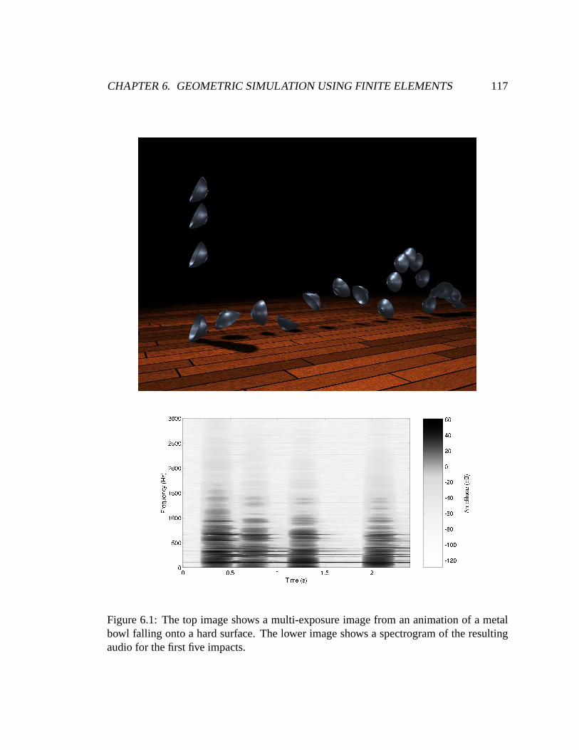
CHAPTER 6. GEOMETRIC SIMULATION USING FINITE ELEMENTS 117
Figure 6.1: The top image shows a multi-exposure image from an animation of a metalbowl falling onto a hard surface. The lower image shows a spectrogram of the resultingaudio for the first five impacts.

CHAPTER 6. GEOMETRIC SIMULATION USING FINITE ELEMENTS 118
The bowl’s shape is arbitrary and there is no known analytical solution for its vibra-
tional modes. The bowl could also be replaced with an arbitrary shape without additional
work. This generality is a clear advantage over banded waveguides.
However this generality entails cost beyond increased computation time. In addition,
the conditions of stability (of error accumulation), convergence (approaching a stable
solution in the limit of infinitesimal elements) and consistency (converges to the correct
differential equation) have to be satisfied, which can be non-trivial or laborious to check
[5]. In case of banded waveguides, the stability condition is checked easily by calcu-
lating the loop gains. The response converges and is consistent in the sense that modal
parameters have been chosen to that end. By the asymptotic and lumped properties the
banded waveguide does not necessarily converge to the detailed dynamics though it does
converge to a continuous wave-propagation solution of the WKB type (as has been shown
in section 3.8.3).
A verification of the finite element method used has been performed and is described
in detail in [135].
Of particular interest is the simulation of a vibraphone bar that has been tuned by
undercutting. A mesh has been constructed (see Figure 2.5) based on the bar also used in
the measurements presented in section 4.1.2.
The undercutting results in a change in transverse impedance between the thin and
thick portions of the bar, which prevents an analytical solution. Two simulations of the
bar have been computed with mesh resolutions of1 cm and2 cm, and compared them
to a recording of a real bar being struck. (The1 cm mesh is shown in Figure 3.) To
facilitate the comparison, the simulated audio was warped linearly in frequency to align
the first partials to that of the real bar at187Hz ( F]3), which is equivalent to adjusting
the simulated bar’s density so that it matches the real bar. The results of this comparison

CHAPTER 6. GEOMETRIC SIMULATION USING FINITE ELEMENTS 119
0 2 4 6 8 10 12 14−20
−10
0
10
20
30
40
50
60
70
Frequency (Normalized)
Am
plitu
de (
dB)
Simulated 1 Simulated 2 Measured Perfect Tuning
Figure 6.2: The top image plots a comparison between the spectra of a real vibraphone bar(Measured), and simulated results for a low-resolution (Simulated 1) and high-resolutionmesh (Simulated 2). The vertical lines located at 1, 4, and 10 show the tuning ratiosreported in [70].
are shown in figure 6.2. Although both the simulated and real bars differ slightly from
the ideal tuning, they are quite similar to each other. All three sounds also contain a
low frequency component below the bar’s first mode that is created by the interaction
with the real or simulated supports. The discrepancy here is of interest mostly because it
highlights the fact that the results of finite element methods depend on the detail of the
model description and the accuracy of the mesh. Scatterings at impedance changes are

CHAPTER 6. GEOMETRIC SIMULATION USING FINITE ELEMENTS 120
Figure 6.3: These figures show a round weight being dropped onto two different surfaces.The surface shown in (a) is rigid while the one shown in (b) is more compliant.
Figure 6.4: A slightly bowed sheet being bent back and forth.
implicitly solved for and carried through, whereas in banded waveguide simulation these
scatterings would either have to be explicitly added or neglected.
Finally I would like to mention examples which are not directly possible using banded
waveguides but can be achieved directly using the finite element method discussed here.
Because the finite element method does not make additional assumptions about how
waves travel in the solid objects, it can be used with nonlinear simulation methods to
generate sounds for objects whose internal vibrations are not modeled by the linear wave

CHAPTER 6. GEOMETRIC SIMULATION USING FINITE ELEMENTS 121
Example Figure Time-step Nodes Elements Surface Total Time Audio Time(10−7s) Elements (min) (min)
Bowl 6.1 10 387 1081 742 91.3 4.01 4.4%Clampled Bar [135, 5] 1 125 265 246 240.4 1.26 0.5%Square Plate [135, 6.a] 10 688 1864 1372 245.0 8.14 3.3%(on center)Square Plate [135, 6.b] 10 688 1864 1372 195.7 7.23 3.7%(off center)Vibraphone Bar 6.2 1 539 1484 994 1309.7 5.31 0.4%Swinging Bar [135, 8] 3 130 281 254 88.4 1.42 1.6%Rigid Sheet 6.3.a 6 727 1954 1438 1041.8 7.80 0.7%Compliant Sheet 6.3.b 20 727 1954 1438 313.1 7.71 2.5%Bent Sheet 6.4 1 678 1838 1350 1574.2 6.45 0.4%
Table 6.1: Computation times for the finite element simulations. The total times indicatethe total number of minutes required to compute one second of simulated data, includinggraphics and file I/O. The audio times listed indicate the amount of the total time thatwas spent generating audio, including related file I/O. The percentages listed indicate thetime spent generating audio as a percentage of the total simulation time. Timing data weremeasured on an SGI Origin using one 350 MHz MIPS R12K processor while unrelatedprocesses were running on the machine’s other processors.
equation. The finite element method we are using employs a nonlinear strain metric
that is suitable for modeling large deformations. Figure 6.3 shows frames from two
animation of a ball dropping onto a sheet. In the first one, the sheet is nearly rigid and
the ball rolls off. In the second animation, the sheet is highly compliant and it undergoes
large deformations as it interacts with the ball. Another example demonstrating large
deformations is shown in figure 6.4 where a slightly bowed sheet is being bent back and
forth to create a crinkling sound. Animations containing the audio for these, and other,
examples have been included on the proceedings video tape and DVD of [135].
All simulations times, including the examples discussed here and those discussed in
[135], are listed in table 6.1. As can be seen, none of the rendered examples is close to
real-time performance. This is true even for simple examples as a clamped uniform bar.
This has to do with the small time-steps required for stability (which in some examples
is smaller than perceptually necessary) in this method but largely because of the mesh
discretization and the required solution of linear systems equations of related size.

Chapter 7
Conclusions, Future Directions and
Applications
[..] the other is a conclusion.
shewing from various causes why the execution has not been equal to what
the author promised to himself and the publick (sic).1 – Samuel Johnson2
I hate quotations. Tell me what you know. – Ralph Waldo Emerson3
Don’t let it end like this. Tell them I said something. – (maybe not the) last
words of Pancho Villa4
1First half of the quote to be found in the introduction chapter.2James Boswell, “Life of Samuel Johnson,” (1755) available athttp://newark.rutgers.edu/
˜jlynch/Texts/BLJ/blj55.html or according to [147, p. 371, q. 17] in vol. 1, p. 292 (1755)3In “Journals of Ralph Waldo Emerson”, Houghton Mifflin Company, Boston, vol. 8, May 3, (1849),
last entry.4Though this quote is usually attributed to Villa on many web-pages, online information by the Tucson-
Pima public library claims no. Seehttp://www.lib.ci.tucson.az.us/government/infoline/archivesq15.htm . K. S. Guthke (in “Last Words,” Princeton University Press, p. 10, (1992)) is undecidedand writes: “Whether authentic or not, this often-cited remark pointedly plays up the collective fascinationwith last words.”
122

CHAPTER 7. CONCLUSIONS, FUTURE DIRECTIONS AND APPLICATIONS123
7.1 Conclusions
The principle of closed wavetrains, also known as the principle of equal phase closure
has been one of the main guiding principles for the work in this thesis.
By using closed wavetrains as a starting point, the resulting simulations and the de-
scriptive dynamics give insights into the dynamics of musical instruments, the connection
between modal synthesis [1], digtal waveguide filter synthesis [187] and simulation based
on finite difference or finite elements. In this concluding notes, I would like to again
highlight the connections that have been made through that guiding principle.
7.2 Separation of Wavetrains and Geometry
Digital waveguide filters assume that the propagation speed of traveling waves is roughly
the same for all frequencies. Small deviations can be implemented using all-pass filters
but large deviations require high-order filters and the extension becomes computationally
expensive. This is equivalent to having one equal phase condition for all frequencies.
The effect is that all modes come about from the same closed wavetrain. As part of this
thesis, I showed that modeling one closed wavetrain per associated mode allows modeling
stiff systems, like bars, which don’t have a constant propagation speed (section 4.1 and
[60]). This separation of wavetrains has a second effect. It also allows for modes to arise
from different, independent paths. This is crucial to allow the idea to be used on dynamic
systems of higher dimensions like membranes, cymbals, or wine glasses (sections 4.2-4.4
and [62, 179]).
A square membrane can serve as illustration of this concept. The first mode corre-
sponds to the family of rays which bounce at the boundary at a 45 degree angle (or a total
of 90 degrees between incoming and outgoing ray). As can easily be seen in Figure 7.1

CHAPTER 7. CONCLUSIONS, FUTURE DIRECTIONS AND APPLICATIONS124
Figure 7.1: Left: Closed paths with one reflection at each side. Right: Closed paths withtwo reflection at the top and bottom and one at the sides.
all of the rays have the same length (the length of twice the diagonal), the same number of
boundary reflections (one on each side). The second mode is the result of rays bouncing
twice at the top and bottom and once on the sides. Again, the family of rays has the
same length and number of reflections. These are two distinct closed paths on the domain
leading to two distinct closed wavetrains and two contributions to the modal response.
The modes are not necessarily unique, however. If accurate modeling is the goal, these de-
generate modes have to be taken into account. If the propagation speed on the medium is
the same on both paths, a condition which is necessarily true in a homogeneous medium,
the two paths may in fact also dynamically be indistinguishable. In this case the necessary
care corresponds to noting, that even though the traveling paths have the same length and
speed, the interaction points may be distinct, as the paths are geometrically different.
If this is being taken care of this mode can in fact be modeled as a “fused” banded
wavepath. If the paths are distinguishable, this does not necessarily require separating
the wavepaths, though that is a possibility. It still requires only that the interaction points
are appropriately adjusted according to the separate wavepath geometries. This is of

CHAPTER 7. CONCLUSIONS, FUTURE DIRECTIONS AND APPLICATIONS125
course the case only if there are no local scatterings, they are weak and can be ignored
or not significant for a dynamic response of interest. The efficiency of waveguide style
simulation is directly connected to the amount of modeled local scatterings. This can be
seen from Bilbao’s work on the connection of finite differencing and digital waveguide
networks [16, 17, 18]. This suggests that considering the perceptual and dynamical
relevance of scatterings is important when trying to achieve efficient models.
7.3 The Link Between Lumped Modal Synthesis and Dig-
ital Waveguide Synthesis
Adrien proposed an interpretive link between additive sinusoidal modeling and physical
modeling by giving additive sinusoids the physical interpretation of damped harmonic
oscillators (mass-spring-damper system) which correspond to the eigensolutions of the
actual physical system and the finite differencing scheme [1]. However, the point then
was, that physical modeling was understood as finite differencing and that modes corre-
sponded to decaying sinusoids.
Banded waveguides provide a similar interpretive link between modal synthesis and
digital waveguide filters. The key here is again the equivalence between the principle
of closed wavetrains and modal response. In essence, the principle explains how modes
come about dynamically, whereas in Adrien’s picture modes are solutions of the govern-
ing equations without a clear dynamic connection.
While previously we have discussed banded waveguides as a generalization of digital
waveguide filters for arbitrary linearly propagating media, banded waveguides can also
be viewed as generalized modal models. The bandpass filters correspond to the resonant
filters of a lumped modal model and the delays correspond to a “phase-delay correction”

CHAPTER 7. CONCLUSIONS, FUTURE DIRECTIONS AND APPLICATIONS126
for the mode. That is in the lumped modal model, the spatial information has been
discarded and aspects of this spatial information is restored using banded waveguides.
Dynamically this can be seen as the time for a wave to travel one cycle to finally close
onto itself. This delay has been discarded in the lumped model and hence transients are
expected to be less accurate in lumped models.
7.4 The Link Between Geometry and Modes
As mentioned before, the connection between closed wavetrain paths and modes leads
to an immediate consideration of geometry. If the underlying dynamics is fixed, then
indeed the resulting modes directly depend on the geometry of the object. This direct
connection was highlighted by Kac’s famous question “Can we hear the shape of a
drum?” [97]. While this question has been answered with “no” for specific nonsmooth
constructions [57], the question remains open for most and very general classes of shapes
(like all smooth boundaries). Of course, one can reinterpret Kac’s question as referring
to perceptual equivalence between shapes rather than mathematical equivalence. This
question has started to get attention in the Computer Music community recently [168].
7.4.1 Geometry, Modes and Efficiency
The reason why the link between modes and geometry is relevant for physical models
of musical instruments has to do with the efficiency gap between modal, waveguide and
banded waveguide models, and mesh-based models like waveguide networks or finite
element methods. The first class of methods is independent of the spatial resolution of
the simulation [62]. The efficiency of the second is dependent on the number of mesh
points. The first class is however dependent on the number of perceptually relevant
CHAPTER 7. CONCLUSIONS, FUTURE DIRECTIONS AND APPLICATIONS127
modes. If this number gets too high, the method becomes inefficient. Hence there is
a trade-off between these two dimensions, which was first observed by Serafin and co-
workers, who proposed a hybrid method to accommodate high densities of modes by
modeling those regions with meshes of low spatial cost and low density regions in the
spectrum using the banded waveguide method [179]. But even in the case of low mode
density, the connection between modes and geometry remains an important one. One
could imagine using a banded waveguide approach blindly, that is, just as a form of phase-
corrected modal model, where the tuning parameters of the banded waveguides, band-
center frequency and delay-length are derived from measurements or precomputation.
Then the interpretation of spatial interaction away from the measurement point would
disappear, an aspect that is very important in the dynamic simulation of many musical
instruments (for the complex interaction with the Indian Tabla drums see [62]).
7.5 Summary
The summary of all these connections can be seen in figure 7.2. By generalizing both
waveguides and modal synthesis, banded waveguides overcome the respective limitations
of media/material type and interaction type. While finite element methods are slow,
they are the solution of choice for complex and highly non-linear media as well as for
arbitrarily complex geometries.

CHAPTER 7. CONCLUSIONS, FUTURE DIRECTIONS AND APPLICATIONS128
Figure 7.2: Comparison of modal synthesis, waveguides, banded waveguides and finiteelement methods.
7.6 Future Work
7.6.1 Perceptual Measures for Synthesis Methods
An interesting and important question has not been thoroughly addressed in this thesis:
the question of a quantitative measure of perceptual quality of a sound simulation. Per-
ceptual models have a history of research behind them [26, 130], though only recently
in the context of digital speech coding for wireless telephony [4, 11, 164] led attempts
at using them to arrive at quantitative measures. Another field where perceptual models
have found an application is music coding for compression (for a review see [144]). This
work has let to a wealth of experimental data which can be used as reference for recorded
music quality and in fact has been used to validate computational model measures by
Thiede and Kabot [196]. While this line of research definitely shows promise for the
use with synthesis methods, it does not directly address a number of specific problems.
In particular the focus of the mentioned work is that differences are imperceptible. In
simulation other determinants of quality may be more desirable. For instance, a simu-
lation may sound different from an actual instrument from which its model parameters

CHAPTER 7. CONCLUSIONS, FUTURE DIRECTIONS AND APPLICATIONS129
have been derived as long as it is “believable” to the listener as being such an instrument
(assuming ignorance of the listener of the original instrument). In fact, Bonebright and
co-workers realized the multiplicity of perceptual qualities when proposing methods for
evaluating such qualities [19].
The perceptual dimension indeed has received some attention in very recent history
in the physical modeling community [95, 168].
I would like to propose taking the perceptual quality coding of Thiede and Kabot
as starting point but extending such a model to a “believability” measure by adding a
judgment of closeness in timbre space [43, chap. 7]. If a quantitative measure along this
lines or in other forms is possible, it still remains to be explored.
7.6.2 Waveguide Preconditioning for Matrix Methods
As seen in section 5.5, delay operations can be seen as a special type of matrix mul-
tiplication. A subdiagonal unitary matrix can be implemented using queues and the
multiplication (rather the shift operation that corresponds to the multiplication) can be
performed inO(1) and maintains this performance if no more than constant of the re-
sulting vector elements are observed at any time-step. Hence if the latter condition holds
one might assume that, given the original matrix or subspaces thereof can be brought
into subdiagonal form, that solution beyondO(N) are possible. This field remains to be
explored, and I just want to mention a number of guiding intuitions.
If indeed subspaces of this type can be found, then they should correspond to a scatter-
free dynamics. In such cases performance enhancing preconditioning is possible without
approximation. Another approach would be to identify scatterings, define a measure of
the strength of the scattering and discard “weak scatterings” to achieve sparsing heuris-
tics. Finally, an approach that is widely used in waveguide modeling is commutation. If

CHAPTER 7. CONCLUSIONS, FUTURE DIRECTIONS AND APPLICATIONS130
The observation points can be fixed, then the behavior between those points in a linear
dynamics can be commuted and can also be commuted into the observation or interaction
operations. Also the effect of “limited observation” that is imposed by the condition of
efficiency is worthy of exploration.
7.6.3 Multirate Banded Waveguides, Perturbations and Extensions
in the Banded Case
Also largely unexplored is the study of perturbations to ideal banded waveguide paths. In
particular there exist literature which study specific modifications to standard waveguides
which should be applicable to the banded waveguide case. For instance in this thesis
rate decimation (multirate modeling, critical sampling in time) was not discussed. Such
approaches have been proposed and implemented in the context of waveguides [206,
180]. Though it should be noted that time-decimation may or may not yield performance
gain [9]. All these questions remain to be explored.

Appendix A
Glossary for Terms in Asymptotic and
Traveling Wave Methods
The purpose of this glossary is mostly to facilitate the reading of related literature for
readers who are not familiar with the nomenclature as it is not part of conventional
textbooks in the computer music and signal processing community.
As introductory books introducing the topic I recommend mostly Brack and Bhaduri’s
recent textbook [25] which guides the mathematics with physical intuition and Dahlen
and Tromp [50] who despite treating seismological problems explain the method in a
way that is appealing to engineers in general. Bouche, Molinet and Mittra [23] provide a
gentle applied mathematics perspective with emphasis on optics and electromagnetism.
Classical texts include Olver [139], Bender and Orszag [13]. Cvitanovic et al [48]
provide a comprehensive treatment, though with emphasis on chaos. More advanced
mathematical texts include Fedoryuk [68], Mishchenkoet al [129], Kravtsov and Orlov
[110] and Kozlov and Treshchev [109]. A related text in pure mathematics treating the
scattering problem is Melrose [128].
131

APPENDIX A. GLOSSARY FOR ASYMPTOTICS TERMS 132
Asymptotics an Ansatz that approaches the exact solution in the limit of some vari-
able. More precisely the generalized Poincare definition of asymptotics is:f (z) =
∑n−1s=0 asφs(z) + O(φn(z)) with (z→ c in R) for all non-negativen with c being a
finite limit point, f (z) being the exact function,φ(z) being the asymptotic sequence
andas being asymptotic amplitudes (from [139, p. 25, eq. (10.03)], which in the
case of a ray asymptotics (here I write the Keller-asymptotics [104, eq. (3)] has
the formu = ∑Nj=1eikSj [A j +O(1/k)] with k being the wave-number andSj andA j
being phase and amplitude. Obviously the expansion is a good one ask→ ∞, that
is for short wave-lengths. See also WKB.
Caustics usually higher dimensional turning points [103, p. 492].
Conjugate points see turning points [25, p. 79].
EBK short for Einstein-Brillouin-Keller [103, p. 493] [25, pp. 78-82], corresponds
to the derivation of the Maslov index by finding closed windings around anN-
torus, whereN is the number of dimensions of the dynamic space. For membranes
and other two-dimensional structures the 2-torus looks like a doughnut. See also
resonant torus.
JWKB short for Jeffreys-Wenzel-Kramers-Brillouin [121, p. 27], same as WKB.
Lagrangian manifold a topological structure in phase-space that relates the dynamics
of the system to the occurance of caustics in physical space [58] also [129, P. 28],
[110, p. 15].
LG approximation short for Liouville-Green approximation [139, p. 190 and 228] al-
ternative term for WKB or JWKB. Refers to the exponential Ansatz in the absence
of turning point treatment which is attributed to Liouville (1837) and Green (1837)
APPENDIX A. GLOSSARY FOR ASYMPTOTICS TERMS 133
though earlier work is traced to Carlini in 1817. JWKB and also Gans (1915) and
Rayleigh [160] treated approximate connection formulas across turning points.
Maslov index counts the number of turning points [25, p. 77] and other phase correc-
tions along a periodic orbit [25, p. 218].
Mode-ray duality also eigenvalue-periodic orbits duality [48, pp. 131ff] the correspon-
dence of modes to closed ray-paths [50, chap. 12].
Periodic orbit a dynamic trajectory that closes onto itself [109, p. 53] or [48]. The
periodic orbit condition [48, p. 259] corresponds to the principle of equal phase
closure.
Principle of equal phase closurerefers to the condition that a taveling wave, following
a closed trajectory, has to return to it’s initial phase at the starting point for reso-
nance to occur [25, p. 79] or [47, 126].
Principle of wavetrain closure same as the principle of equal phase closure.
Quasi-periodic orbits is an orbit on an integrable domain (and hence on the EBK reso-
nant torus) which does not close onto itself in finite length [25, p. 92].
Resonant torus is the topological structure which can be constructed using canonical
transforms for integrable dynamical systems and which lead to EBK quantization
conditions [25, p. 78ff] and are used in the study of chaos [25, p. 98].
Stationary points see turning points [205, p. 11].
Turning points points at which WKB becomes invalid due to singularity [13, p. 497],
similar to caustics, though it also refers to boundaries that induce phase-shifts [25,

APPENDIX A. GLOSSARY FOR ASYMPTOTICS TERMS 134
p.434]. Caustic turning points inside the domain are also referred to as “smooth”
turning points and fixed boundaries are referred to as “hard” turning points [25, p.
88].
Winding number number of windings along a topological dimension of the EBKN-
torus [25, p. 81].
WKB short for Wenzel-Kramers-Brillouin [13, p. 486] [121, p. 27] but going back
to Rayleigh [160] (see [13, p. 486]) and Jeffreys (see [13, p. 486][121, p. 27]).
Wigner-Kramers-Brillouin [25, p. 63]. Refers to the traveling wave Ansatz to solve
differential equations. Specifically, Olver [139] defines WKB to refer to this Ansatz
in the presence of treatement across turning points. See also LG approximation.

Appendix B
Implementation
All application examples have been implemented within the framework of the synthesis
toolkit (STK) developed by Perry R. Cook and Gary Scavone and is available with Perry
Cook’s recent book [45] and online athttp://www-ccrma.stanford.edu/software/
stk/ .
STK uses C++ for implementation of the synthesis algorihms. Graphical user inter-
faces are provided using Tcl/tk. In addition, STK provides an input interface for MIDI.
The core routine to be performed at every time step is exactly the banded waveguide
structure of Figure 1.1.
The primitives used in this filter diagram are implemented using already existing
classes in STK. Each banded wave-path is constructed from a second-order resonant filter
(BiQuad.cpp ) and a delay-line (Delay.cpp ). The free parameters are the length of the
delay-line and the three filter coefficients of the second-order infinite impulse response
filter [193]:
135

APPENDIX B. IMPLEMENTATION 136
yt = A0xt +(2Rcosθ)yt−1−R2yt−2 (B.1)
These then can be recalculated to gain, resonant frequency and bandwidth [194, p.
92]:
R≈ 1−B/2 (B.2)
cosθ =2R
1+R2 cosω (B.3)
A0 = (1−R2)sinθ (B.4)
The the overall delayd in feedback (forming a comb filter structure[194]) shows a
harmonic resonant response and fundamental frequencyf0 and harmonicsfm correspond
to the delay lengthd:
fm =m·Nr
dm∈ N+
0 (B.5)
whereNr is the sampling rate. The resonant frequency and one resonant peak of the
of the comb filter must coincide as they both follow from the same closure condition.
Usually the resonant filter frequency is tuned using modal esimation and the multi-
valuedness of B.5 by knowing the quotient of propagation speedcn to path lengthl . This
can be derived from equations 3.11 and 3.12 as the delay lengthd∗n is calculated from this
quotient plus the sampling rate:

APPENDIX B. IMPLEMENTATION 137
d∗n =l ·Nr
cn(B.6)
The bandwidth of the resonant filter is a non-physical parameter and defines the
spectral neighborhood of a mode. In general a fairly wide bandwidth is used as the actual
frequency response is achieved throught the closure condition of the wave-path (compare
section 4.1).
The sum of all wave-paths defines both the output as well as the interaction point. This
point can be used for impulsive excitations or can be fed into an interaction algoritm. In
our implementation the bow excitation algorithm (BowTabl ) provided by STK is used.
The collection of all these parameters then can be controlled either via MIDI or
through a graphical user interface as depicted in Figure B.1. This example shows the
graphical user interface written in Tcl/TK for the one-dimensional and quasi-one-dimensional
instruments discussed in this thesis.

APPENDIX B. IMPLEMENTATION 138
Figure B.1: STK graphical user interface for bars and bowls using banded waveguides.

139
To none more grateful than to me; escaped
From the vast city, where I long had pined
A discontented sojourner; now free,
Free as a bird to settle where I will. – William Wordsworth 1
1In “The Prelude,” bk. 1, l. 1, (1850) according to [147, p. 746, q. 17]

Index of Authors
Abel, J. S. 107, 160Abrahams, I. D. 22, 152Ade, G. 5Adrien, J.-M. 10, 18, 123, 125, 145Aird, M. 60, 145Akay, A. 20, 22, 145Alwan, A. 128, 145Ames, W. F. 9, 14, 118, 145Artuso, R. 7, 33, 43, 51, 131, 133, 149Askenfelt, A. 9, 14, 61, 147, 148Avanzini, F. 13, 48, 99, 145
Back, A. D. 107, 145Bank, B. 10, 13, 48, 99, 130, 145, 146Batterman, R. W. 43, 146Becker, E. E. 22, 161Beerends, J. G. 128, 146Begault, D. R. 9, 48, 50, 146Bender, C. M. 43, 131, 133, 134, 146Berry, M. 43, 146Bhaduri, R. K. 43, 48, 49, 51, 91, 94,
131–134, 147Bilbao, S. D. 9, 57, 60, 125, 146Birkhoff, G. D. 42Bonebright, T. L. 129, 146Borin, G. 13, 48, 99, 145Bork, I. 9, 14, 60, 146Bornemann, F. A. 16, 147, 159Bouche, D. 43, 131, 147Boyd, J. P. 43, 147
Brack, M. 43, 48, 49, 51, 91, 94, 131–134,147
Bregman, A. S. 128, 147Bretos, J. 9, 14, 60, 147Brillouin, L. 45, 52, 132, 134Browne, S. 9, 147Browning, R. ivBucur, V. 60, 147
Cadoz, C. 9, 14, 113, 147, 151Carlbom, I. 25, 151Carlini, F. 133Caudell, T. P. 129, 146Cavagnero, M. 56, 147Cavaliere, S. 107, 150Chaigne, A. xiii, 9, 14–16, 60–62, 107,
146–149, 154, 158Chan, R. H. 17, 109, 148Chapman, S. J. 43, 148Chen, G. 42, 49, 148Chladni, E. F. F. 21, 148Cho, M. I. 107, 148Coleman, M. P. 42, 49, 148Cook, P. R. 3, 4, 10, 20, 27, 28, 60, 61, 71,
72, 105, 108, 111, 118, 121, 123, 126,127, 135, 148, 150, 153, 156
Coppens, A. B. 114, 153Cremer, L. 28, 41, 61, 62, 65, 67, 133, 149Cunningham, S. J. 5Cvitanovic, P. 7, 33, 43, 51, 131, 133, 149
Dahl, L. 107, 149
140

INDEX OF AUTHORS 141
Dahlen, F. A. 43, 131, 133, 149Dahlqvist, P. 7, 33, 43, 51, 131, 133, 149Daubechies, I. 8, 149Davenport, G. 111Davidson, P. 4, 153De Poli, G. 13, 48, 99, 145Decker, S. L. 9, 153Denissenko, P. 22, 149DiFilippo, D. K., D. Pai 20, 149Dirac, P. A. M. 23Dodge, C. 9, 10, 149Doutaut, V. xiii, 9, 14–16, 60, 62, 107,
148, 149Driscoll, T. A. 126, 149Duistermaat, J. J. 8, 43, 132, 149Dutilleux, P. 48, 158
Eichler, M. 6, 150Einstein, A. 52, 132Elko, G. 25, 151Emerson, R. W. 122Essl, G. 3, 4, 27, 28, 60, 61, 71, 72, 105,
108, 111, 118, 121, 123, 126, 127, 150,153, 156
Evangelista, G. 107, 150
Feiten, B. 9, 14, 154Fenny, B. 21, 22, 97, 150Flannery, B. P. 16, 17, 157Fletcher, N. H. xvii, 60, 72, 74, 119, 150Florens, J.-L. 9, 14, 113, 147, 151Fontana, F. 13, 48, 99, 145Frey, A. R. 114, 153Friedlander, F. G. 21, 41, 151Fulling, S. A. 43, 151Funkhouser, T. 25, 151
Gaida, E. 95Galilei, G. 21Gans, R. 133Gardner, W. G. 9, 151Goethe, J. W. von 59, 111
Goldsmith, T. E. 129, 146Golub, G. H. 16, 110, 151Green, G. 132Guran, A. 21, 22, 97, 150
Hadas, M. 103Hanson, F. B. 43, 151Harma, A. 106, 151Heckl, M. 28, 41, 62, 65, 133, 149Heckl, M. A. 22, 152Hekstra, A. P. 128, 146Helmholtz, H. L. F. 21, 152Hinrichs, N. 21, 22, 97, 150, 152Hodgins, J. K. 112, 156Hollier, M. P. 128, 146, 158Holz, D. 60, 152Howls, C. J. 43, 152Hsieh, D. Y. 22, 149Huang, P. 123, 127, 159Huang, X. Y. 22, 152Huopaniemi, J. 9, 48, 152, 159
Ibrahim, R. A. 22, 152Ingard, K. U. 10, 53, 155
Jaffe, D. 8, 105, 152Jarvelainen, H. 13, 106, 129, 153, 157Jeffreys, H. 132Jerse, T. A. 9, 10, 149Johnson, D. H. 106, 156, 160Johnson, S. 1, 122Joly, P. 14, 158Jot, J.-M. 107, 149
Kabot, E. 128, 160Kac, M. 126, 153Kapur, A. 4, 87, 88, 153Karjalainen, M. 8, 10, 13, 36, 48, 99, 106,
153, 154, 157, 161Karplus, K. 8, 153Keller, J. B. xvi, 8, 21, 41–45, 48, 49, 52,
91–93, 132, 153Kendall, G. S. 9, 153

INDEX OF AUTHORS 142
Kinsler, L. E. 114, 153Kosfelder, M. 9, 14, 60, 146Kovintavewat, P. 107, 153Kozlov, V. V. 42, 131, 133, 154Kramers, H. A. 45, 134Krause, R. 16, 147Kravtsov, Y. A. 8, 43, 92, 131, 132, 154Kreyszig, E. 11, 46, 154Kry, P. G. 18, 20, 27, 103, 161Kurz, M. 9, 14, 154
Laakso, T. I. 13, 36, 154Laine, U. K. 13, 36, 106, 151, 154Laird, J. 60, 145Lambourg, C. 14, 148, 154Lang, M. xvi, 106, 154Lansky, P. 106, 154Lauterborn, W. 21, 155Lawry, J. M. H. 43, 148Lec, S. J. 103Legge, K. A. 60, 157Liouville, J. 132Lokki, T. 9, 159Luciani, A. 9, 14, 113, 147
Mainieri, R. 7, 33, 43, 51, 131, 133, 149Makila, P. M. 107, 154Makur, A. 107, 155Martens, W. L. 9, 153Mathews, J. 132, 134, 155Matignon, D. 14, 60, 149, 154Maynard, J. D. 5McIntyre, M. E. 8, 26, 61, 66, 155McMillan, A. J. 22, 155Mead, D. J. 7, 41, 133, 155Melrose, R. B. 131, 155Migliori, A. 5Miner, N. E. 129, 146Mishchenko, A. S. 43, 131, 132, 155Mitra, S. K. 107, 148, 155Mittra, R. 43, 131, 147Molinet, F. 43, 131, 147
Moore, B. C. J. 128, 155Moore, J. L. 60, 66, 155Moral, J. A. 9, 14, 60, 147Morse, P. M. 10, 53, 155Muller, G. 21, 155
Narayanan, S. 128, 145Ng, C. 97, 163Ng, M. K. 17, 109, 148
O’Brien, J. F. 3, 27, 108, 111, 112, 118,121, 155, 156
Ockendon, J. R. 43, 148Oden, J. T. 22, 161Oestreich, M. 22, 152Olivera e Silva, T. 106, 156Olver, F. W. J. 7, 42, 43, 46, 131, 132, 134,
156Oppenheim, A. V. 20, 33, 34, 106, 156,
160Orduna Bustamante, F. 60, 156Orlov, Y. I. 8, 43, 92, 131, 132, 154Orszag, S. A. 43, 131, 133, 134, 146Ottaviani, L. 126, 129, 158
Paatero, T. 106, 151, 157Pai, D. K. 10, 18, 20, 27, 60, 103, 158,
161, 162Painter, T. 128, 156Paladin, A. 105, 156Palumbi, M. 9, 14, 61, 156Partington, J. R. 107, 154Penttinen, H. 106, 157Petrolito, J 60, 157Pillot, D. 9, 14, 60, 146Pingali, G. 25, 151Pitteroff, R. 21, 157Pivin, D. P. 51, 157Pohlmann, K. C. 13, 157Popp, K. 21, 22, 97, 150, 152Press, W. H. 16, 17, 157Puckette, M. 48, 160

INDEX OF AUTHORS 143
Rabenstein, R. 18, 157, 161Raman, C. V. 21, 157Rayleigh, J. W. S. 21, 133, 134, 157Ree, S. 51, 158Reichl, L. E. 51, 158Rhaouti, L. 14, 158Richmond, J. L. 20, 158Rix, A. W. 128, 146, 158Roads, C. 6, 8, 10, 19, 158Rocchesso, D. 13, 48, 99, 105, 126, 129,
145, 156, 158Rodet, X. 61, 159Rossing, T. D. xv–xvii, 21, 60, 61, 72, 74,
87–89, 94–96, 119, 150, 158, 159Rubinow, S. I. xvi, 42, 44, 45, 48, 49,
91–93, 132, 153Ruiz, P. M. 9, 14, 159Russell, B. 23, 103
Sanders, J. V. 114, 153Santamarıa, C. 9, 14, 60, 147Savioja, L. 9, 107, 159Scalcon, F. 105, 158Schafer, R. W. 20, 33, 34, 156Schiela, A. 16, 159Schiff, L. I. 44, 159Schroeder, M. 9Schumacher, R. T. 8, 26, 61, 66, 155Seno, L. 9, 14, 61, 156Serafin, S. 21, 49, 61, 97, 123, 127, 130,
159, 163Serra, X. 10, 18, 60, 159Shatalov, V. E. 43, 131, 132, 155Shen, A. 128, 145Smith, J. 105, 162Smith, J. H. 21, 61, 159Smith, J. O. xiii, 8–10, 14, 21, 26, 29, 41,
43, 48, 49, 57, 61, 66, 104, 105, 107,123, 127, 130, 152, 158–160, 162
Sondhi, M. M. 25, 151Spanias, A. 128, 156
Stam, J. 16, 160Stautner, J. 48, 160Steiglitz, K. 9–11, 33, 35, 50, 106, 135,
136, 154, 156, 160Sternin, B. Y. 43, 131, 132, 155Strong, A. 8, 153Strope, B. 128, 145Sullivan, C. R. 8, 160
Tanner, G. 7, 33, 43, 51, 131, 133, 149Taylor, R. L. 9, 14, 163Teukolsky, S. A. 16, 17, 157Tew, R. H. 43, 148Thiede, T. 128, 160Thomsen, J. J. 22, 160Tolonen, T. 8, 10, 13, 48, 99, 130, 153, 161Trautmann, L. 18, 157, 161Trebuchet, L.-C. 9, 14, 60, 146Trefethen, L. N. 9, 161Treshchev, D. V. 42, 131, 133, 154Tromp, J. 43, 131, 133, 149Truax, B. 6, 161Tsoi, A. C. 107, 145Twain, M. 59Tworzydlo, W. W. 22, 161
Ungar, E. 28, 41, 62, 65, 133, 149
Vaananen 9, 159Vaidyanathan, P. P. 16, 34, 161Valimaki, V. 8, 10, 13, 36, 48, 99, 107,
130, 153, 154, 159, 161van den Doel, K. 10, 18, 20, 27, 60, 100,
103, 161, 162van Duyne, S. 9, 14, 105, 162Van Loan, C. F. 16, 110, 151Vattay, G. 7, 33, 43, 51, 131, 133, 149Vergez, C. 61, 159Vetterling, W. T. 16, 17, 157Villa, P. 122Volpert, A. I. 42, 162Volpert, Vitaly A. 42, 162

INDEX OF AUTHORS 144
Volpert, Vladimir A. 42, 162Von Schroeter, T. 106, 162
Wagner, C. 16, 162Walker, R. L. 132, 134, 155Waller, M. D. 21, 61, 162Wawrzynek, J. 10, 18, 19, 60, 162Wenzel, G. 45, 134Wesseling, P. 16, 162West, J. 25, 151
Whelan, N. 7, 33, 43, 51, 131, 133, 149Wilkerson, C. 97, 163Wirzba, A. 7, 33, 43, 51, 131, 133, 149Woodhouse, J. 8, 21, 26, 61, 66, 155, 157,
159Wordsworth, W. 139
Zhou, J. 42, 49, 148Zienkiewicz, O. C. 9, 14, 163

Bibliography
[1] J.-M. Adrien. The missing link: Modal synthesis. In G. De Poli, A. Piccialli, andC. Roads, editors,Representations of Musical Signals, chapter 8, pages 269–297.MIT Press, Cambridge, 1991.
[2] M. Aird and J. Laird. Extending Digital Waveguides to Include MaterialModelling. InProceedings of the COST G-6 Conference on Digital Audio Effects(DAFX-01), Limerick, Ireland, December 6-8 2001.
[3] A. Akay. Acoustics of friction. Journal of the Acoustical Society of America,111(4):1525–1548, April 2002.
[4] A. Alwan, S. Narayanan, B. Strope, and A. Shen. Speech Production andPerception Models and Their Applications to Synthesis, Recognition, and Coding.In Proceedings of the International Symposiun of Signals, Systems, and Electronics(ISSSE-95), pages 367–372, October 1995.
[5] W. F. Ames. Numerical Methods for Partial Differential Equations. AcademicPress, San Diego, 3 edition, 1992.
[6] F. Avanzini, B. Bank, G. Borin, G. De Poli, F. Fontana, and D. Rocchesso. Musicalinstrument modeling: the case of the piano. InProceedings of the Workshopon Current Research Directions in Computer Music, Barcelona, November 15-17 2001. Available online:http://www.iua.upf.es/mtg/mosart/paper/p18.pdf .
[7] A. D. Back and A. C. Tsoi. Nonlinear System Identification Using DiscreteLaguerre Functions.Journal of Systems Engineering, 6(3):194–207, August 1996.
[8] B. Bank. Physics-Based Sound Synthesis of the Piano. Master’s thesis, BudapestUniversity of Technology and Economics, 2000. Also available at HelsinkiUniversity of Technology, Laboratory of Acoustics and Audio Signal Processing,Report 54.
145

BIBLIOGRAPHY 146
[9] B. Bank. Accurate and efficient modeling of beating and two-stage decay forstring instrument synthesis. InProceedings of the MOSART Workshop on CurrentResearch Directions in Computer Music, pages 134–137, Barcelona, Spain, 2001.
[10] R. W. Batterman.The Devil in the Details. Oxford University Press, 2002.
[11] J. G. Beerends, A. P. Hekstra, A. W. Rix, and M. P. Hollier. PerceptualEvaluation of Speech Quality (PESQ), the new ITU standard for end-to-endspeech quality assessment. Part II — Psychoacoustic Model. Unpublishedmanuscript. Psytechnics reference number 2001-P03b. Available at:http://www.psytechnics.com/papers/2001-P03b.pdf , July 2001.
[12] D. R. Begault. 3-D Sound for Virtual Reality and Multimedia. Academic Press,1994.
[13] C. M. Bender and S. A. Orszag.Advanced Mathematical Methods for Scientistsand Engineers. McGraw-Hill, 1978.
[14] M. Berry. Why are special functions special?Physics Today, 54(4):11–12, April2001.
[15] M. Berry. Singular Limits.Physics Today, 55(5):10–11, May 2002.
[16] S. D. Bilbao. Digital Waveguide Networks as Multidimensional Wave DigitalFilters. In Proceedings of the COST G-6 Conference on Digital Audio Effects(DAFX-00), pages 49–54, Verona, Italy, December 7-9 2000.
[17] S. D. Bilbao. Digital Waveguide Networks for Inhomogeneous Media. InProceedings of the COST G-6 Conference on Digital Audio Effects (DAFX-00),pages 249–252, Verona, Italy, December 7-9 2000.
[18] S. D. Bilbao. Wave and Scattering Methods for the Numerical Integration ofPartial Differential Equations. PhD thesis, Stanford University, May 2001.
[19] T. L. Bonebright, N. E. Miner, T. E. Goldsmith, and T. P. Caudell. Data Collectionand Analysis Techniques for Evaluating the Perceptual Qualities of AuditoryStimuli. In Proceedings of the International Conference of Auditory Display(ICAD’98), http://www.ewic.org.uk/ewic/workshop/view.cfm/ICAD-98 ,1998.
[20] I. Bork. Practical Tuning of Xylophone Bars and Resonators.Applied Acoustics,46:103–127, 1995.
[21] I. Bork, A. Chaigne, L.-C. Trebuchet, M. Kosfelder, and D. Pillot. Comparisonbetween Modal Analysis and Finite Element Modelling of a Marimba Bar.Acustica united with acta acustica, 85(2):258–266, 1999.

BIBLIOGRAPHY 147
[22] F. A. Bornemann and R. Krause. Classical and Cascadic Multigrid — AMethodological Comparison. In P. E. Bjørstad, M. S. Espedal, and D. E.Keyes, editors,Proceedings of the 9th International Conference on DomainDecomposition Methods 1996, Ullensvang, Norway, chapter 7, pages 64–71.Domain Decomposition Press, 1998.
[23] D. Bouche, F. Molinet, and R. Mittra.Asymptotic Methods in Electromagnetics.Springer Verlag, 1997.
[24] J. P. Boyd. The Devil’s Invention: Asymptotic, Superasymptotic andHyperasymptotic Series.Acta Applicandae, 56:1–98, 1999.
[25] M. Brack and R. K. Bhaduri.Semiclassical Physics, volume 96 ofFrontiers inPhysics. Addison-Wesley Publishing, 1997.
[26] A. S. Bregman.Auditory Scene Analysis. MIT Press, Cambridge, Massachusetts,1990.
[27] J. Bretos, C. Santamarıa, and J. A. Moral. Finite element analysis and experimentalmeasurements of natural eigenmodes and random responses of wooden bars usedin musical instruments.Applied Acoustics, 56:141–156, 1999.
[28] S. Browne. Hybrid Reverberation Algorithm using Truncated Impulse ResponseConvolution and Recursive Filtering. Master’s thesis, University of Miami, CoralGables, Florida, June 2001.
[29] V. Bucur. Acoustics of Wood. CRC Press, Boca Raton, 1995.
[30] C. Cadoz, A. Luciani, and J.-L. Florens. Responsive Input Devices and SoundSynthesis by Simulation of Instrumental Mechanisms: The Cordis System.Computer Music Journal, 8(3):60–73, 1984.
[31] C. Cadoz, A. Luciani, and J.-L. Florens. CORDIS-ANIMA: A Modeling andSimulation System for Sound and Image Synthesis - The General Formalism.Computer Music Journal, 17(1):19–29, Spring 1993.
[32] M. Cavagnero. Addendum to JWKB. Unpublished lecture notes available on-line athttp://www.pa.uky.edu/˜mike/courses/phy614/html/pdf/addend.pdf , April 29 2002.
[33] A. Chaigne and A. Askenfelt. Numerical simulations of piano strings. I. A physicalmodel for a struck string using finite difference methods.Journal of the AcousticalSociety of America, 95(2):1112–1118, 1994.

BIBLIOGRAPHY 148
[34] A. Chaigne and A. Askenfelt. Numerical simulations of piano strings. II.Comparisons with measurements and systematic exploration of some hammer-string parameters.Journal of the Acoustical Society of America, 95(3):1631–1640,1994.
[35] A. Chaigne and V. Doutaut. Numerical simulations of xylophones. I. Time-domainmodeling of the vibrating bars.Journal of the Acoustical Society of America,101(1):539–557, 1997.
[36] A. Chaigne and C. Lambourg. Time-domain simulation of damped impactedplates. I. Theory and experiments.Journal of the Acoustical Society of America,109(4):1422–1432, April 2001.
[37] R. H. Chan and M. K. Ng. Iterative Methods for Linear Systems with MatrixStructure. In T. Kailath and A. Sayed, editors,Fast Reliable Algorithms forMatrices with Structure, pages 117–152. SIAM, 1999.
[38] S. J. Chapman, J. M. H. Lawry, J. R. Ockendon, and R. H. Tew. On the Theory ofComplex Rays.SIAM Review, 41(3):417–509, 1999.
[39] G. Chen, M. P. Coleman, and J. Zhou. Analysis of Vibration Eigenfrequencies of aThin Plate by the Keller-Rubinow Wave Method I: Clamped Boundary ConditionsWith Rectangular or Circular Geometry.SIAM Journal on Applied Mathematics,51(4):967–983, August 1991.
[40] E. F. F. Chladni.Die Akustik. Breitkopf & Hartel, Leipzig, Germany, 1830.
[41] M. I. Cho and S. K. Mitra. Warped Discrete Cosine Transform and Its Applicationin Image Compression.IEEE Transactions on Circuits and Systems for VideoTechnology, 10(8):1364–1373, December 2000.
[42] P. R. Cook. Physically Informed Sonic Modeling (PhISM): Synthesis of PercussiveSounds.Computer Music Journal, 21(3):38–49, 1997.
[43] P. R. Cook, editor. Music Cognition, and Computerized Sound. MIT Press,Cambridge, Massachusetts, 1999.
[44] P. R. Cook. Toward Physically-Informed Parametric Synthesis of Sound Effects.In Proceedings of the 1999 IEEE Workshop on Applications of Signal Processingto Audio and Acoustics (WASPAA-99), pages 1–5, New Paltz, NY, October 17-201999.
[45] P. R. Cook.Real Sound Synthesis for Interactive Applications. A K Peters, Ltd.,July 2002.

BIBLIOGRAPHY 149
[46] L. Cremer.The Physics of the Violin. MIT Press, Cambridge, 1984.
[47] L. Cremer, M. Heckl, and E. Ungar.Structure-Borne Sound. Springer Verlag, 2ndedition, 1988.
[48] P. Cvitanovic, R. Artuso, P. Dahlqvist, R. Mainieri, G. Tanner, G. Vattay,N. Whelan, and A. Wirzba.Classical and Quantum Chaos. Webbook, January30 2002. version 9.1.1 available online athttp://www.nbi.dk/ChaosBook/ .
[49] L. Dahl and J.-M. Jot. A Reverberator Based on Absorbent All-Pass Filters. InProceedings of the COST G-6 Conference on Digital Audio Effects (DAFX-00),pages 67–72, Verona, Italy, December 7-9 2000.
[50] F. A. Dahlen and J. Tromp.Theoretical Global Seismology. Princeton UniversityPress, 1998.
[51] I. Daubechies. Where do wavelets come from? — A personal point of view.Proceedings of the IEEE — Special Issue on Wavelets, 84(4):510–513, April 1996.
[52] P. Denissenko and D. Y. Hsieh. Surface water waves interaction in a circular vesselwith oscillating walls. InDivision for Fluid Dynamics (DFD98) Meeting of TheAmerican Physical Society (abstract only), Philadelphia, PA., November 22-241998.
[53] P. Denissenko and D. Y. Hsieh. Water Waves in a Circular Elastic Vessel: TheExperiiment. Online document to abstract only conference contribution [52],November 1998.
[54] D. K. DiFilippo, D. Pai. Contact Interaction with Integrated Audio and Haptics. InProceedings of the International Conference on Auditory Display (ICAD), 2000.
[55] C. Dodge and T. A. Jerse.Computer Music: Synthesis, Composition, andPerformance. Schirmer Books, 1985.
[56] V. Doutaut, D. Matignon, and A. Chaigne. Numerical simulations of xylophones.II. Time-domain modeling of the resonator and of the radiated sound pressure.Journal of the Acoustical Society of America, 104(3):1633–1647, 1998.
[57] T. A. Driscoll. Eigenmodes of Isospectral Drums.SIAM Review, 39(1):1–17,March 1997.
[58] J. J. Duistermaat. Book Review - Lagrangian Manifolds and the Maslov operator.Bulletin of the American Mathematical Society, 27(1):174–179, July 1992.

BIBLIOGRAPHY 150
[59] M. Eichler. On Finding One’s Way in the Uncharted Swamps of Interdisciplinarity.In Outside the Lines: Issues in Interdisciplinary Research, pages 58–62. McGill-Queen’s University Press, 1996.
[60] G. Essl and P. R. Cook. Banded Waveguides: Towards Physical Modeling ofBowed Bar Percussion Instruments. InProceedings of the International ComputerMusic Conference (ICMC), pages 321–324, Beijing, China, 1999. InternationalComputer Music Association (ICMA).
[61] G. Essl and P. R. Cook. Measurements and efficient simulations of bowed bars.Journal of the Acoustical Society of America, 108(1):379–388, 2000.
[62] G. Essl and P. R. Cook. Sound Propagation Modeling in Objects: Rubbing, Slidingand Scratching the Surface. Unpublised manuscript, available by request from thefirst author., November 2001.
[63] G. Essl and P. R. Cook. Banded Waveguides on Circular Topologies and ofBeating Modes: Tibetan Singing Bowls and Glass Harmonicas. Submitted to theInternational Computer Music Conference (ICMC-02), Goteborg, Sweden., 2002.
[64] G. Essl and P. R. Cook. The Principle of Closed Wavetrains, Resonance andEfficiency: The Missing Link Revisited. Submitted to the International ComputerMusic Conference (ICMC-02), Goteborg, Sweden., 2002.
[65] G. Evangelista. Real-Time Time-Varying Frequency Warping via Short-TimeLaguerre Transform. InProceedings of COST G-6 Conference on Digital AudioEffects (DAFX-00), pages 7–12, Verona, Italy, December 2000.
[66] G. Evangelista and S. Cavaliere. Representation and Modification of Time-VaryingSound Signals. InProceedings of the 13th Colloquium on Musical Informatics,pages 25–28, L’Aquila, Italy, September 2000.
[67] G. Evangelista and S. Cavaliere. Signal Transforms for the Detection andIdentification of Signals. InProceedings of EUSIPCO 2000, pages 1069–1072,Tampere, Finland, September 2000.
[68] M. V. Fedoryuk, editor. Partial Differential Equations V: Asymptotic Methodsfor Partial Differential Equations, volume 34 ofEncyclopaedia of MathematicalSciences. Springer Verlag, 1999.
[69] B. Fenny, A. Guran, N. Hinrichs, and K. Popp. A historical review on dry frictionand stick-slip phenomena.Applied Mechanics Review, 51(5):321–341, May 1998.
[70] N. H. Fletcher and T. D. Rossing.The Physics of Musical Instruments. SpringerVerlag, New York, 2 edition, 1998.

BIBLIOGRAPHY 151
[71] J.-L. Florens and C. Cadoz. The Physical Model: Modeling and Simulatingthe Instrumental Universe. In G. De Poli, A. Piccialli, and C. Roads, editors,Representations of Musical Signals, chapter 7, pages 227–268. MIT Press,Cambridge, 1991.
[72] F. G. Friedlander. On the Oscillations of a Bowed String.Proceedings of theCambridge Philosophical Society, 49(3):516–530, 1952.
[73] S. A. Fulling. Reflections on the Role of Asymptotic Analysis in Physics.In A. Semikhatov, M. Vasiliev, and V. Zaikin, editors,Proceedings of theInternational Conference on Quantization, Gauge Theory and Strings, pages 307–315, Moscow, 2001. Scientific World.
[74] T. Funkhouser, I. Carlbom, G. Elko, G. Pingali, M. M. Sondhi, and J. West. Abeam tracing approach to acoustic modeling for interactive virtual environments.In Proceedings of SIGGRAPH 98, Computer Graphics Proceedings, AnnualConference Series, pages 21–32, July 1998.
[75] W. G. Gardner. A Realtime Multichannel Room Simulator. InProceedings ofthe 124th meeting of the Acoustical Society of America, New Orleans, November1992.
[76] W. G. Gardner. The Virtual Acoustic Room. Master’s thesis, MassachusettsInstitute of Technology, Cambridge, MA, September 1992.
[77] G. H. Golub and C. F. Van Loan.Matrix Computations. Johns Hopkins UniversityPress, Baltimore, Maryland, third edition, 1996.
[78] F. B. Hanson. Singular Point and Exponential Asymptotics. In R. Wong, editor,Asymptotics and Computational Analysis, volume 124 ofLecture Notes in Pureand Applied Mathematics, pages 211–240. Marcel Dekker, Inc., 1990.
[79] A. Harma. Frequency-Warped Autoregressive Modeling and Filtering. PhD thesis,Helsinki University of Technology, Espoo, Finland, May 2001. Also available asTechnical Report 61 from the same institution.
[80] A. Harma and U. K. Laine. A Comparison of Warped and Conventional LinearPredictive Coding.IEEE Transactions on Speech and Audio Processing, 9(5):579–588, July 2001.
[81] A. Harma and T. Paatero. Discrete Representation of Signals on a LogarithmicFrequency Scale. InProceedings of the IEEE Workshop on Applications of SignalProcessing to Audio and Acoustics (WASPAA-01), pages 39–42, New Paltz, NewYork, October 21-14 2001. IEEE Signal Processing Society.

BIBLIOGRAPHY 152
[82] M. A. Heckl. Curve Squeal of Train Wheels, Part 2: Which Wheel Modes areProne to Squeal?Journal of Sound and Vibration, 229(3):695–707, 2000.
[83] M. A. Heckl and I. D. Abrahams. Active Control of Friction-Driven Oscillations.Journal of Sound and Vibration, 193(1):417–426, 1996.
[84] M. A. Heckl and I. D. Abrahams. Curve Squeal of Train Wheels, Part 1:Mathematical Model for its Generation. Journal of Sound and Vibration,229(3):669–693, 2000.
[85] M. A. Heckl and X. Y. Huang. Curve Squeal of Train Wheels, Part 3: ActiveControl. Journal of Sound and Vibration, 229(3):709–735, 2000.
[86] H. L. F. Helmholtz.On the Sensations of Tone. Dover, 1885/1954.
[87] N. Hinrichs, M. Oestreich, and K. Popp. On the Modelling of Friction Oscillators.Journal of Sound and Vibration, 216(3):435–459, 1998.
[88] D. Holz. Acoustically important properties of xylophone-bar materials: Cantropical woods be replaced by European species?Acustica united with actaacustica, 82(6):878–884, 1996.
[89] C. J. Howls. Development of Exponential and Hyper-asymptotics. In C. J. Howls,T. Kawai, and Y. Takei, editors,Toward the Exact WKB Analysis of DifferentialEquations, Linear or Non-Linear. Kyoto University Press, 2000.
[90] J. Huopaniemi.Virtual Acoustics and 3-D Sound in Multimedia Signal Processing.PhD thesis, Helsinki University of Technology, Espoo, Finland, November 1999.Also available at Helsinki University of Technology, Laboratory of Acoustics andAudio Signal Processing, Report 53.
[91] C. Hutchins and V. Benade, editors.Research Papers in Violin Acoustics 1975-1993. Acoustical Society of America, Woodbury, 1997.
[92] R. A. Ibrahim. Friction-induced vibration, chatter, squeal, and chaos Part I:Mechanics of contact and friction.Applied Mechanics Review, 47(7):209–226,July 1994.
[93] R. A. Ibrahim. Friction-induced vibration, chatter, squeal, and chaos Part II:Dynamics and modeling.Applied Mechanics Review, 47(7):227–253, July 1994.
[94] D. Jaffe and J. O. Smith. Extensions of the Karplus-Strong plucked stringalgorithm.Computer Music Journal, 7(2):56–69, 1983.
BIBLIOGRAPHY 153
[95] H. Jarvelainen. Applying perceptual knowledge to string instrument synthesis. InProceedings of the Workshop on Current Research Directions in Computer Music,Barcelona, November 15-17 2001. Available online:http://www.iua.upf.es/mtg/mosart/paper/p09.pdf .
[96] H. Jarvelainen, V. Valimaki, and M. Karjalainen. Audibility of the timbral effectsof inharmonicity in stringed instrument tones.Acoustics Research Letters Online,2(3):79–84, April 2001.
[97] M. Kac. Can One Hear the Shape of a Drum?American Mathematical Monthly,73(4):1–23, April 1966.
[98] A. Kapur, G. Essl, P. Davidson, and P. R. Cook. The Electronic Tabla Controller. InProceedings of the 2002 Conference on New Instruments for Musical Expression(NIME-02), pages 77–81, Dublin, Ireland, May 24-26 2002.
[99] M. Karjalainen, V. Valimaki, and T. Tolonen. Plucked-String Models: From theKarplus-Strong Algorithm to Digital Waveguides and Beyond.Computer MusicJournal, 22(3):17–32, 1998.
[100] K. Karplus and A. Strong. Digital synthesis of plucked string and drum timbres.Computer Music Journal, 7(2):43–55, 1983.
[101] J. B. Keller. Bowing of Violin Strings.Communications on Pure and AppliedMathematics, 6:483–495, 1953.
[102] J. B. Keller. A Geometrical Theory of Diffraction. In L. M. Graves, editor,Proceedings of Symposia in Applied Mathematics, volume 8, pages 27–52.American Mathematical Society, 1958.
[103] J. B. Keller. Semiclassical Mechanics.SIAM Review, 27(4):485–504, December1985.
[104] J. B. Keller and S. I. Rubinow. Asymtotic Solution of Eigenvalue Problems.Annalsof Physics, 9:24–75, 1960.
[105] G. S. Kendall, W. L. Martens, and S. L. Decker. Spatial Reverberation: Discussionand Demonstration. In M. V. Mathews and J. R. Pierce, editors,Current Directionsin Computer Music, chapter 7, pages 65–87. MIT Press, 1991.
[106] L. E. Kinsler, A. R. Frey, A. B. Coppens, and J. V. Sanders.Fundamentals ofAcoustics. John Wiley and Sons, Inc., New York, fourth edition edition, 2000.
[107] P. Kovintavewat. Modeling the Impulse Response of an Office Room. Master’sthesis, Chalmers University of Technology, 1998.

BIBLIOGRAPHY 154
[108] V. V. Kozlov. Symmetries, Topology, and Resonances in Hamiltonian Mechanics,volume 31 ofA Series of Modern Surveys in Mathematics, Series 3.SpringerVerlag, 1996.
[109] V. V. Kozlov and D. V. Treshchev. Billiards - A Genetic Introduction to theDynamics of Systems with Impacts, volume 89 ofTranslations of MathematicalMonographs. American Mathematical Society, 1991.
[110] Y. A. Kravtsov and Y. I. Orlov.Caustics, Catastrophes and Wave Fields, volume 15of Series on Wave Propagation. Springer Verlag, 1993.
[111] E. Kreyszig. Advanced Engineering Mathematics. John Wiley & Sons, Inc.,seventh edition, 1993.
[112] M. Kurz. Klangsynthese mittels physikalisher Modellierung einer schwingendenSaite durch numerische Integration der Differentialgleichung. Master’s thesis,Technical University Berlin, September 1995. In german. See [113] for a conciseEnglish summary.
[113] M. Kurz and B. Feiten. Physical modelling of a striff string by numericalintegration. InProceedings of the International Computer Music Conference(ICMC-96), pages 361–364, Hong Kong, August 19-24 1996.
[114] T. I. Laakso, V. Valimaki, M. Karjalainen, and U. K. Laine. Splitting the UnitDelay: Tools for fractional delay filter design.IEEE Signal Processing Magazine,13(1):30–60, January 1996.
[115] C. Lambourg, A. Chaigne, and D. Matignon. Time-domain simulation of dampedimpacted plates. II. Numerical model and results.Journal of the Acoustical Societyof America, 109(4):1433–1447, April 2001.
[116] M. Lang. Allpass Filter Design and Applications.IEEE Transactions on SignalProcessing, 46(9):2505–2514, September 1998.
[117] P. Lansky and K. Steiglitz. Synthesis of Timbral Families by Warped LinearPrediction.Computer Music Journal, 5(3):45–49, Fall 1981.
[118] P. M. Makila and J. R. Partington. Laguerre and Kautz shift approximations ofdelay systems.International Journal of Control, 72(10):932–946, 1999.
[119] P. M. Makila and J. R. Partington. Shift Operator Induced Approximations ofDelay Systems.SIAM Journal on Control and Optimization, 37(6):1897–1912,1999.

BIBLIOGRAPHY 155
[120] A. Makur and S. K. Mitra. Warped Discrete-Fourier Transform: Theory andApplications.IEEE Transactions on Circuits and Systems - I: Fundamental Theoryand Applications, 48(9):1086–1093, September 2001.
[121] J. Mathews and R. L. Walker.Mathematical Methods of Physics. W. A. Benjamin,Inc., second edition, 1970.
[122] M. E. McIntyre, R. T. Schumacher, and J. Woodhouse. On the oscillation ofmusical instruments.Journal of the Acoustical Society of America, 74(5):1325–1344, 1983.
[123] A. J. McMillan. A Non-Linear Friction Model for Self-Excited Vibrations.Journalof Sound and Vibration, 205(3):323–335, 1997.
[124] D. J. Mead. Wave Propagation and Natural Modes in Periodic Systems: I. Mono-Coupled Systems.Journal of Sound and Vibration, 40(1):1–18, 1975.
[125] D. J. Mead. Wave Propagation and Natural Modes in Periodic Systems: II. Multi-Coupled Systems, With and Without Damping.Journal of Sound and Vibration,40(1):19–39, 1975.
[126] D. J. Mead. Waves and Modes in Finite Beams: Application of the Phase-ClosurePrinciple.Journal of Sound and Vibration, 171(5):695–702, 1994.
[127] D. J. Mead. Wave Propagation in Continuous Periodic Structures: ResearchContributions from Southampton 1964-1995.Journal of Sound and Vibration,190(3):495–524, 1996.
[128] R. B. Melrose.Geometric Scattering Theory. Cambridge University Press, 1995.
[129] A. S. Mishchenko, V. E. Shatalov, and B. Y. Sternin.Lagrangian Manifolds andthe Maslov Operator. Springer Verlag, 1990.
[130] B. C. J. Moore.An Introduction to the Psychology of Hearing. Academic Press,4th edition, 1997.
[131] J. L. Moore. Acoustics of Bar Percussion Instruments. PhD thesis, Ohio StateUniversity, Columbus, 1970.
[132] P. M. Morse and K. U. Ingard.Theoretical Acoustics. Princeton University Press,Princeton, NJ, 1968.
[133] G. Muller and W. Lauterborn. The Bowed String as a Nonlinear DynamicalSystem.Acustica, 82(4):657–664, 1996.
[134] J. F. O’Brien. private communication, 2001.

BIBLIOGRAPHY 156
[135] J. F. O’Brien, P. R. Cook, and G. Essl. Synthesizing Sounds from Physically BasedMotion. In Proceedings of SIGGRAPH 2001, Computer Graphics Proceedings,Annual Conference Series, pages 529–536, August 2001.
[136] J. F. O’Brien and J. K. Hodgins. Graphical modeling and animation of brittlefracture. InProceedings of SIGGRAPH 99, Computer Graphics Proceedings,Annual Conference Series, pages 137–146, August 1999.
[137] J. F. O’Brien and J. K. Hodgins. Animating fracture.Communications of the ACM,43(7):68–75, July 2000.
[138] T. Olivera e Silva. On the Design of Linear-in-the-Parameters Adaptive Filters.In Proceedings of the 5th International Conference on Electronics, Circuits andSystems, volume 1, pages 385–388. IEEE, 1998.
[139] F. W. J. Olver.Asymptotics and Spectial Functions. Academic Press, 1974.
[140] A. V. Oppenheim and D. H. Johnson. Discrete Representation of Signals.Proceedings of the IEEE, June 1972.
[141] A. V. Oppenheim, D. H. Johnson, and K. Steiglitz. Computation of Spectra withUnequal Resolution Using the Fast Fourier Transform.Proceedings of the IEEE,59(2):299–301, February 1971.
[142] A. V. Oppenheim and R. W. Schafer.Discrete-Time Signal Processing. PrenticeHall, 1989.
[143] F. Orduna Bustamante. Nonuniform beams with harmonically related overtonesfor use in percussion instruments.Journal of the Acoustical Society of America,90(6):2935–2941, 1991. Erratum: Journal of the Acoustical Society of America91(6), 3582–3583 (1992).
[144] T. Painter and A. Spanias. Perceptual Coding of Digital Audio.Proceedings of theIEEE, 88(4):451–513, April 2000.
[145] A. Paladin and D. Rocchesso. A Dispersive Resonator in Real Time on MARSWorkstation. InProceedings of the International Computer Music Conference(ICMC-92), pages 146–149, 1992.
[146] M. Palumbi and L. Seno. Physical modeling by directly solving wave PDE. InProceedings of the International Computer Music Conference (ICMC), pages 325–328, Beijing, China, 1999. International Computer Music Association (ICMA).
[147] A. Partington, editor.The Oxford Dictionary of Quotations. Oxford UniversityPress, revised 4th edition, 1996.

BIBLIOGRAPHY 157
[148] H. Penttinen, M. Karjalainen, T. Paatero, and H. Jarvelainen. New techniques tomodel reverberant instrument body responses. InProceedings of the InternationalComputer Music Conference (ICMC-2001), Havana, Cuba, September 17-232001.
[149] J. Petrolito and K. A. Legge. Optimal undercuts for the tuning of percussion beams.Journal of the Acoustical Society of America, 102(4):2432–2437, 1997.
[150] R. Pitteroff. Contact mechanics of the bowed string. PhD thesis, University ofCambridge, Cambridge, UK., 1995. Also published in a series of papers in anarchival journals [151, 152, 153].
[151] R. Pitteroff and J. Woodhouse. Mechanics of the Contact Area Between a ViolinBow and a String. Part I: Reflection and Transmission Behaviour.Acustica unitedwith acta acustica, 84(3):543–562, 1998.
[152] R. Pitteroff and J. Woodhouse. Mechanics of the Contact Area Between a ViolinBow and a String. Part II: Simulating the Bowed String.Acustica united with actaacustica, 84(4):744–757, 1998.
[153] R. Pitteroff and J. Woodhouse. Mechanics of the Contact Area Between a ViolinBow and a String. Part III: Parameter Dependence.Acustica united with actaacustica, 84(5):929–946, 1998.
[154] D. P. Pivin. Semiclassical Periodic Orbit Theory and Possible Application to OpenQuantum Ballistic Cavities. Unpublished manuscript available online athttp://www.eas.asu.edu/˜pivin/Comps/pot.pdf , November 1997.
[155] K. C. Pohlmann.Principles of Digital Audio. McGraw-Hill, third edition, 1995.
[156] W. H. Press, S. A. Teukolsky, W. T. Vetterling, and B. P. Flannery.NumericalRecipes in C. Cabridge University Press, second edition, 1992.
[157] R. Rabenstein and L. Trautmann. Digital Sound Synthesis by Physical Modelling.In Proceedings of the Symposion on Image and Signal processing and Analysis(ISPA’01), Pula, Croatia, June 2001.
[158] C. V. Raman. Scientific Papers of C. V. Raman, volume 2 – Acoustics. IndianAcademy of Sciences, Bangalore, India, 1988.
[159] J. W. S. Rayleigh.The Theory of Sound, volume 1&2. Dover, 1894/1945.
[160] J. W. S. Rayleigh. On the Propagation of Waves through a Stratified Medium,with Special Reference to the Question of Reflection.Proceedings of the RoyalSociety of London. Series A, Containing Papers of a Mathematical and PhysicalCharacter, 86(586):207–226, Februrary 1912.
BIBLIOGRAPHY 158
[161] S. Ree and L. E. Reichl. Classical and quantum chaos in a circular billiard with astraight cut.Physical Review E, 60(2):1607–1615, August 1999.
[162] L. Rhaouti, A. Chaigne, and P. Joly. Time-domain modeling and numericalsimulation of a kettledrum. Journal of the Acoustical Society of America,105(6):3545–3562, June 1999.
[163] J. L. Richmond and D. K. Pai. Robotic measurement and modeling of contactsounds. InProceedings of the International Conference on Auditory Display(ICAD), 2000.
[164] A. W. Rix and M. P. Hollier. The Perceptual Analysis Measurement Systemfor Robust End-to-End Speech Quality Assessment. InProceedings of theInternational Conference on Acoustics, Speech and Signal Processing (ICASSP-00), June 5-9 2000.
[165] C. Roads.The Computer Music Tutorial. MIT Press, 1996.
[166] D. Rocchesso. The Ball within the Box: a sound-processing metaphor.ComputerMusic Journal, 19(4):47–57, Winter 1995.
[167] D. Rocchesso and P. Dutilleux. Generalization of a 3-D Acoustic Resonator Modelfor the Simulation of Spherical Enclosures.Applied Signal Processing, 1:15–26,2001.
[168] D. Rocchesso and L. Ottaviani. Can One Hear the Volume of a Shape? InProceedings of the 2001 IEEE Workshop on Applications of Signal Processing toAudio and Acoustics, pages 115–118, New Paltz, NY, October 21-24 2001. IEEESignal Processing Society.
[169] D. Rocchesso and F. Scalcon. Accurate Dispersion Simulation for Piano Strings.In Proceedings of the Nordic Acoustical Meeting (NAM-96), pages 407–414,Helsinki, Finland, June 12-14 1996.
[170] D. Rocchesso and J. O. Smith. Circulant and Elliptic Feedback Delay Networksfor Artificial Reverberation.IEEE Transaction on Speech and Audio, 5(1):51–60,January 1996.
[171] T. D. Rossing. Acoustics of percussion instruments – Part I.The Physics Teacher,14:546–556, 1976.
[172] T. D. Rossing. Acoustics of the glass harmonica.Journal of the Acoustical Societyof America, 95(2):1106–1111, 1994.

BIBLIOGRAPHY 159
[173] T. D. Rossing.Science of Percussion Instruments, volume 3 ofSeries In PopularScience. World Scientific Publishing, 2000.
[174] P. M. Ruiz. A Technique for Simulating the Vibrations of Strings with a DigitalComputer. Master’s thesis, University of Illinois, 1969.
[175] L. Savioja, J. Huopaniemi, T. Lokki, and Vaananen. Virtual environmentsimulation - advances in the DIVA project. InProceedings of the InternationalConference on Auditory Display (ICAD), pages 43–46, 1997.
[176] L. Savioja and V. Valimaki. Reducing the Dispersion Error in the DigitalWaveguide Mesh Using Interpolation and Frequency-Warping Techniques.IEEETransaction on Speech and Audio Processing, 8(2):184–194, March 2000.
[177] A. Schiela and F. A. Bornemann. Sparsing in Real Time Simulation. Unpublisedmanuscript available athttp://www-m3.ma.tum.de/m3/ftp/Bornemann/pdf/sparsing.pdf , May 2002.
[178] L. I. Schiff. Quantum Mechanics. McGraw-Hill, New York, second edition, 1955.
[179] S. Serafin, P. Huang, and J. O. Smith. The Banded Digital Waveguide Mesh. InProceedings of the Workshop on Current Research Directions in Computer Music,Barcelona, November 15-17 2001. Available online:http://www.iua.upf.es/mtg/mosart/paper/p38.pdf .
[180] S. Serafin and J. O. Smith. A Multirate, Finite-Width, Bow-String InteractionModel. In Proceedings of the COST G-6 Conference on Digital Audio Effects(DAFX-00), pages 207–210, Verona, Italy, December 7-9 2000.
[181] S. Serafin, C. Vergez, and X. Rodet. Friction and Application to Real-timePhysical Modeling of a Violin. InProceedings of the International ComputerMusic Conference (ICMC), pages 216–219, Beijing, China, 1999. InternationalComputer Music Association (ICMA).
[182] X. Serra. A Computer Model for Bar Percussion Instruments. InProc.International Computer Music Conference (ICMC), pages 257–262, The Hague,1986. International Computer Music Association (ICMA).
[183] J. H. Smith.Stick-Slip Vibration and its Constitutive Laws. PhD thesis, Universityof Cambridge, March 1990.
[184] J. H. Smith and J. Woodhouse. The tribology of rosin.Journal of the Mechanicsand Physics of Solids, 48(8):1633–1681, August 2000.

BIBLIOGRAPHY 160
[185] J. O. Smith.Techniques for Digital Filter Design and System Identification withApplication to the Violin. PhD thesis, Stanford University, Stanford, California,1983. Also available as technical report from Stanford Center for ComputerResearch in Music and Acoustics (CCRMA) Department of Music Report No.STAN-M-14.
[186] J. O. Smith. Efficient Simulation of the Reed-Bore and Bow-String Mechanisms.In Proceedings of the International Computer Music Conference (ICMC), pages275–280, The Hague, 1986. International Computer Music Association (ICMA).
[187] J. O. Smith. Physical Modeling Synthesis Update.Computer Music Journal,20(2):44–56, 1996.
[188] J. O. Smith. Digital Waveguide Modeling of Musical Instruments. draft ofunpublished online manuscript, available athttp://ccrma-www.stanford.edu/˜jos/waveguide/ , 2002.
[189] J. O. Smith and J. S. Abel. Bark and ERB Bilinear Transforms.IEEE Transactionson Speech and Audio Processing, 7(6):697–708, November 1999.
[190] J. Stam.Multi-Scale Stochastic Modelling of Complex Natural Phenomena. PhDthesis, University of Toronto, 1995.
[191] J. Stautner and M. Puckette. Designing Multi-Channel Reverberators.ComputerMusic Journal, 6(1):52–65, Spring 1982.
[192] K. Steiglitz. Derivation of frequency warping by contour integrals. Unpublishedmanuscript. Alternate derivation to [141], 1970.
[193] K. Steiglitz. A Note on Constant-Gain Digital Resonators.Computer MusicJournal, 18(4):8–10, 1994.
[194] K. Steiglitz.A Digital Signal Processing Primer. Addison-Wesley, 1996.
[195] C. R. Sullivan. Extending the Karplus-Strong Algorithm to Synthesize ElectricGuitar Timbres with Distortion and Feedback.Computer Music Journal, 14(3):26–37, 1990.
[196] T. Thiede and E. Kabot. A New Perceptual Quality Measure for Bit Rate ReducedAudio. In Proceedings of the 100th AES Convention, Copenhagen, Denmark, May11-14 1996. Preprint 4280.
[197] J. J. Thomsen. Using Fast Vibration to Quench Friction-Induced Oscillations.Journal of Sound and Vibration, 228(5):1079–1102, 1999.

BIBLIOGRAPHY 161
[198] T. Tolonen, V. Valimaki, and M. Karjalainen. Evaluation of Modern SoundSynthesis Methods. Technical Report Laboratory of Acoustics and Audio SignalProcessing, Report 48, Helsinki University of Technology, Epsoo, Finland, March1998.
[199] T. Tolonen, V. Valimaki, and M. Karjalainen. Modeling of Tension ModulationNonlinearity in Plucked Strings. IEEE Transactions on Speech and AudioProcessing, 8(3):300–310, May 2000.
[200] L. Trautmann and R. Rabenstein. Digital Sound Synthesis Based on TransferFunction Models. InProceedings of the 1999 IEEE Workshop on Applicationsof Signal Processing to Audio and Acoustics (WASPAA-99), pages 83–86, NewPaltz, New York, October 17-20 1999.
[201] L. N. Trefethen. Finite Difference and Spectral Methods for Ordinary and PartialDifferential Equations. Available online athttp://web.comlab.ox.ac.uk/oucl/work/nick.trefethen/pdetext.html , 1996.
[202] B. Truax. Computer Music and Acoustic Communication: Two EmergingInterdisciplines. In A. Salter, L. Hearn, editor,Outside the Lines: Issues inInterdisciplinary Research, pages 64–73. McGill-Queen’s University Press, 1996.
[203] W. W. Tworzydlo, E. E. Becker, and J. T. Oden. Numerical modeling offriction-induced vibrations and dynamic instabilities.Applied Mechanics Review,47(7):255–274, July 1994.
[204] P. P. Vaidyanathan.Multirate Systems and Filter Banks. Signal Processing Series.Prentice Hall, 1993.
[205] R. Vaillancourt and A. L. Smirnov, editors.Asymptotic Methods in Mechanics,volume 3 ofCRM Proceedings & Lecture Notes. American Mathematical Society,1993.
[206] V. Valimaki and T. Tolonen. Multirate Extensions for Model-Based Synthesis ofPlucked String Instruments. InProceedings of the International Computer MusicConference (ICMC-97), pages 244–247, Thessaloniki, Greece, September 25-301997.
[207] K. van den Doel.Sound Synthesis for Virtual Reality and Computer Games. PhDthesis, University of British Columbia, Vancouver, Canada, November 1998.
[208] K. van den Doel, P. G. Kry, and D. K. Pai. FoleyAutomatic: Physically-BasedSound Effects for Interactive Simulation and Animation. InProceedings ofSIGGRAPH 2001, Computer Graphics Proceedings, Annual Conference Series,pages 537–544, August 2001.

BIBLIOGRAPHY 162
[209] K. van den Doel and D. K. Pai. Synthesis of shape dependent sounds with physicalmodeling. InProceedings of the International Conference on Auditory Display(ICAD), 1996.
[210] K. van den Doel and D. K. Pai. The Sound of Physical Shapes. Technical report,Dept. of Computer Science, University of British Columbia, Canada, Vancouver,1996.
[211] K. van den Doel and D. K. Pai. The Sound of Physical Shapes.Presence, 7(4):382–395, August 1998.
[212] K. van den Doel and D. K. Pai. Modal Synthesis for ResonatingObjects. Unpublished manuscript available at: urlhttp://www.cs.ubc.ca/ kv-doel/publications/modalpaper.pdf, 2002.
[213] S. van Duyne and J. Smith. A Simplified Approach to Modeling Dispersion Causedby Stiffness in Strings and Plates. InProceedings of the International ComputerMusic Conference (ICMC-94), pages 407–410, 1994.
[214] S. van Duyne and J. O. Smith. Physical Modeling With the 2D Waveguide Mesh.In Proceedings of the International Computer Music Conference (ICMC), pages40–47, The Hague, 1993. International Computer Music Association (ICMA).
[215] A. I. Volpert, V. A. Volpert, and V. A. Volpert. Traveling Wave Solutions ofParabolic Systems, volume 140 ofTranslations of Mathematical Monographs.American Mathematical Society, 1994.
[216] T. Von Schroeter. Frequency Warping with Arbitrary Allpass Maps.IEEE SignalProcessing Letters, 6(5):116–118, May 1999.
[217] C. Wagner. Introduction to Algebraic Multigrid. Course Notes of an AlgebraicMultigrid Course at the University of Heidelberg in Fall of 1998/99:http://www.iwr.uni-heidelberg.de/groups/techsim/chris/amg.pdf , 1998.
[218] M. D. Waller.Chladni Figures — A Study in Symmetry. G. Bell and Sons, London,1961.
[219] J. Wawrzynek. VLSI Models for Sound Synthesis. In M. Mathews and J. Pierce,editors,Current Directions in Computer Music Research, chapter 10, pages 113–148. MIT Press, Cambridge, 1989.
[220] P. Wesseling.An Introduction to Multigrid Methods. John Wiley & Sons, 1991.Also available online at:http://www.mgnet.org/mgnet-books-wesseling.html .

BIBLIOGRAPHY 163
[221] C. Wilkerson, C. Ng, and S. Serafin. The Mutha Rubboard Controller: InteractiveHeritage. InProceedings of the 2002 Conference on New Instruments for MusicalExpression (NIME-02), pages 82–85, Dublin, Ireland, May 24-26 2002.
[222] O. C. Zienkiewicz and R. L. Taylor.The Finite Element Method, volume 1: TheBasis. Butterworth-Heinemann, fifth edition, 2000.
[223] O. C. Zienkiewicz and R. L. Taylor.The Finite Element Method, volume 2: SolidMechanics. Butterworth-Heinemann, fifth edition, 2000.
[224] O. C. Zienkiewicz and R. L. Taylor.The Finite Element Method, volume 3: FluidDynamics. Butterworth-Heinemann, fifth edition, 2000.