physical review d 103531 (2009) dark matter in the solar

Dark matter in the Solar System. I. The distribution function of WIMPsat the Earth from solar capture

Annika H.G. Peter*

Department of Physics, Princeton University, Princeton, New Jersey 08544, USAand California Institute of Technology, Mail Code 105-24, Pasadena, California 91125, USA

(Received 8 February 2009; published 28 May 2009)

The next generation of dark matter (DM) direct detection experiments and neutrino telescopes will

probe large swaths of dark matter parameter space. In order to interpret the signals in these experiments, it

is necessary to have good models of both the halo DM streaming through the Solar System and the

population of DM bound to the Solar System. In this paper, the first in a series of three on DM in the Solar

System, we present simulations of orbits of DM bound to the Solar System by solar capture in a toy solar

system consisting of only the Sun and Jupiter, assuming that DM consists of a single species of weakly

interacting massive particle (WIMP). We describe how the size of the bound WIMP population depends

on the WIMP mass m�, spin-independent cross section �SIp , and spin-dependent cross section �SD

p . Using

a standard description of the Galactic DM halo, we find that the maximum enhancement to the direct

detection event rate, consistent with current experimental constraints on the WIMP-nucleon cross section,

is <1% relative to the event rate from halo WIMPs, while the event rate from neutrinos from WIMP

annihilation in the center of the Earth is unlikely to meet the threshold of next-generation, km3-sized

(IceCube, KM3NeT) neutrino telescopes.

DOI: 10.1103/PhysRevD.79.103531 PACS numbers: 95.35.+d, 95.85.Ry, 96.25.De, 96.60.Vg

I. INTRODUCTION

A. Dark matter and detection

There is overwhelming evidence that nonbaryonic darkmatter (DM) must exist in large quantities in the Universe,yet its nature is unknown. A popular candidate for DM isone or more species of weakly interacting massive particle(WIMP). Particles of this type occur naturally in manytheories of physics beyond the standard model (SM); ex-amples include the neutralino � in supersymmetry [1], the

lightest Kaluza-Klein photon Bð1Þ in universal extra-dimension (UED) theories [2–4], or the heavy photon AH

in Little Higgs models [5–7]. These particular candidatesare all stable, self-annihilating, behave as cold dark matter,and are thermally produced in the early universe in roughlythe amount needed to explain the dark matter [8].

We may expect rapid progress in constraining the natureof DM due to the maturity of a number of technologiestargeting different but complementary WIMP signals. Thenext generation of particle colliders, in particular, theLarge Hadron Collider, may see signatures of physicsbeyond the SM. A new generation of satellites is searchingfor photons (e.g., the Fermi Gamma-Ray Space Telescope[9,10]) and other particles (e.g., ATIC [11], PAMELA [12])resulting from WIMP annihilations in the Milky Way’sDM halo.

There are also experiments to probe the local WIMPpopulation. Since the flux of particles from WIMP annihi-lation scales as the square of the WIMP density, any region

in the Solar System that has an unusually high density ofWIMPs is a good target. WIMPs generically interactwith baryons, which means that WIMPs passing throughthe Solar System may be trapped and settle into densecores in the potential wells of the Sun or the planets.The previous generation of neutrino telescopes (e.g.,BAKSAN [13], MACRO [14], Super-Kamiokande [15],AMANDA [16,17]) places the strongest constraintson the spin-dependent WIMP-proton cross section �SD

p

( & 10�39 cm2 at m� � 100 GeV) based on flux limits of

neutrinos from WIMP annihilation in the Sun and Earth.Even if the next generation of neutrino telescopes withdetector volumes approaching 1 km3 (e.g., Antares [18],IceCube [19], the proposed KM3NeT [20]) do not identifya WIMP annihilation signature, they are projected to im-prove constraints on �SD

p by almost 2 orders of magnitude.

The best limits on the spin-dependent WIMP-neutron�SD

n and spin-independent WIMP-nucleon �SIp cross sec-

tions come from direct detection experiments. The signa-ture of WIMPs in these experiments is a small(� 10 keV� 100 keV) nuclear recoil. The next genera-tion of direct detection experiments is slated to have targetmasses approaching 1000 kg (e.g., DEAP/CLEAN [21],LUX [22], SuperCDMS [23–25], WARP [26], XENON1T[27], XMASS [28]) and to be sensitive to cross sectionsdown to �SI

p � 10�46 cm2, �SDp � 10�40 cm2, and �SD

n �10�42 cm2 [29,30].

B. WIMPs in the Solar System

For a given WIMP model, event rates in direct detectionexperiments and neutrino telescopes are determined by the*[email protected]

PHYSICAL REVIEW D 79, 103531 (2009)

1550-7998=2009=79(10)=103531(44) 103531-1 � 2009 The American Physical Society

http://dx.doi.org/10.1103/PhysRevD.79.103531

phase space distribution function (DF) of WIMPs in theSolar System. The fiducial assumption is that the directdetection event rate andWIMP capture rate in the Earth aredominated by DM particles from the Galactic halo, passingthrough the Solar System on unbound orbits [1,31]. Thereare potentially observable consequences if even a tinyfraction of WIMPs may become captured to the SolarSystem, since bound WIMPs have lower speeds than haloWIMPs. The push for many direct detection experimentsis toward ever-lower nuclear recoil energy thresholds(� 0:1 keV–1 keV), both in order to gain sensitivity tolow-mass WIMPs and because the event rate is muchhigher there than at higher energies [32,33]. At such lowenergies, low-speed WIMPs contribute disproportionatelyto the event rate for kinematic reasons.

Low-speed WIMPs have an even greater impact on theevent rate of neutrinos from annihilation in the Earth. Theshallowness of the Earth’s potential well means that onlylow-speed WIMPs may be captured in the Earth. In par-ticular, if the WIMP mass is above 400 GeV, only WIMPsbound to the Solar System may be trapped in the Earth.

Two processes have been identified by which WIMPsmay become captured to the Solar System at rates largeenough to be important for terrestrial dark matter experi-ments. Gravitational Capture: Gould [34,35] pointed outthat WIMPs may be captured from the halo by gravitation-ally scattering on the planets. By treating WIMP orbits inthe Solar System as a diffusion problem, Gould [35] andLundberg and Edsjo [36] estimated that bound WIMPsdominate the annihilation rate of WIMPs in the Earth forWIMP masses * 100 GeV. Solar Capture: WIMPs cap-tured in the Sun will reach thermal equilibrium with solarnuclei on time scales t� ��1P, where � is the optical depthof the Sun forWIMPs and P is the orbital period of a boundWIMP. However, Damour and Krauss [37] identified apopulation of solar-captured WIMPs that could survivefor much longer periods of time due to a type of secularresonance that pulls their perihelia outside the Sun. Usingsecular perturbation theory, they found that this populationcould produce a low-recoil direct detection rate compa-rable to that of halo WIMPs for �SI

p � 10�42–10�40 cm2,

and could yield an annihilation rate in the Earth a factor of�100 greater than the rate expected from unbound haloWIMPs for WIMP masses �100–150 GeV [38].

While these results are intriguing, the semianalytic treat-ments used in these papers cannot fully capture the richrange of behavior in small-N systems such as the SolarSystem. It is important to check these results with numeri-cal experiments. Moreover, the annihilation rate of WIMPsin the Sun depends critically on whether WIMPs capturedin the Sun thermalize rapidly with solar nuclei. If theplanets can pull the WIMPs out of the Sun for extendedperiods of time, or even eject the particles from the system,the annihilation rate will be depressed with respect tocurrent estimates.

In a set of three papers [39,40], we present simulationsof WIMP orbits in the Solar System, including both thegravitational effects of the dominant planet, Jupiter, and anaccurate Monte Carlo description of WIMP-nucleon elas-tic scattering in the solar interior, as well as a discussion ofthe likely contribution of bound WIMPs to direct detectionexperiments and neutrino telescopes. In this paper, Paper I,we focus on WIMP capture in the Sun. In order to put ourresults in context, we first summarize the treatment ofDamour and Krauss [37], and describe the mechanismthey found that extended the lifetimes of solar-capturedWIMPs in the Solar System and built up the DF of WIMPsat the Earth: the Kozai mechanism.

C. Damour and Krauss (1999) and the Kozaimechanism

In the absence of gravitational torques from the planets,WIMPs captured onto Earth-crossing orbits by elastic scat-tering in the Sun will have a small number density at theEarth relative to the halo number density for two reasons.(i) Unless the WIMP is massive (m� * 1 TeV), the char-

acteristic energy a WIMP loses to a solar nucleus is largeenough such that most captured WIMPs have aphelia thatlie inside the Earth’s orbit. (ii) The characteristic time tothe next scatter, which will almost certainly remove theWIMP from an Earth-crossing orbit unlessm� * 1 TeV, is

of order t / P�=�. For a WIMP with semimajor axis a ¼1 AU, P� ¼ 1 year. If, for example, �SI

p ¼ 10�41 cm2 (or

�SDp ¼ 10�39 cm2), �� 10�3, so the WIMP lifetime in the

Solar System is only of order a thousand years, shortcompared to the age of the Solar System.Damour and Krauss [37] recognized that the lifetimes of

bound WIMPs in Earth-crossing orbits could be extendedby orders of magnitude if gravitational torques from theplanets decreased the WIMP eccentricity (increased theperihelion distance) enough that the WIMP orbit no longerpenetrated the Sun. For WIMPs in planetary systems suchas our own, such behavior is possible if the rate of peri-helion precession _! is small, since then the torques fromthe planets act in a constant direction over many WIMPorbits. This process was first examined by Kozai [41] in thecontext of asteroid orbits and is sometimes called the Kozairesonance. The signature of this resonance is large fluctua-tions in both the inclination and eccentricity while thesemimajor axis is fixed. The Kozai resonance can lead toboth libration and circulation in the argument of perihelion!, and we use the term ‘‘Kozai cycles’’ to describe theseoscillations. Kozai cycles have been studied in the contextof comets [42], asteroids [43,44], triple star systems [45],and exoplanets [46].Damour and Krauss found approximate analytic Kozai

solutions for a solar system containing the inner planetsand Jupiter on circular, coplanar orbits. The requirementthat _! is small means that Kozai cycles are only significantfor WIMPs with perihelia that are not too far inside the

ANNIKA H.G. PETER PHYSICAL REVIEW D 79, 103531 (2009)

103531-2

solar radius, so the solar potential is not far from that of apoint-mass. Damour and Krauss use an analytic approxi-mation to the solar potential in the outer r > 0:55R� of theSun, where R� is the radius of the Sun. They expanded thepotentials of the planets to quadrupole order in the smallparameter aP=a, where aP is the semimajor axis of aplanet, and neglected short-period terms and mean-motionresonances. The solutions have an additional feature—ifthe orbital plane of the planets in the solar system is thex� y plane, the z-component of the specific angular mo-

mentum, Jz ¼ffiffiffiffiffiffiffiffiffiffiffiffiffiffiffiffiffiffiffiffiffiffiffiffiffiffiffiffiffiffiffiGM�að1� e2Þp

cosI (I is the inclination)is a conserved quantity.

To estimate the size of the solar-captured WIMP popu-lation at the Earth, Damour and Krauss made the followingadditional assumptions. (i) Jupiter-crossing WIMPs (withaphelia greater than Jupiter’s semimajor axis, ra > aJ �5:2 AU) were ignored, since their lifetimes in the SolarSystem were assumed to be short. Similarly, all WIMPswith ra < aJ that were not on Kozai cycles were alsoignored. (ii) They assumed that all WIMPs on Kozai cycleswould survive for the lifetime of the Solar System withoutrescattering in the Sun, regardless of the optical depth inthe Sun for WIMPs. Since the typical lifetime of Earth-crossing WIMPs is �103 yr for �SI

p � 10�41 cm2, the ex-

tension of the lifetimes of even a few Earth-crossing par-ticles to the age of the Solar System results in a significantboost to the DF of bound WIMPs at the Earth.

D. This work

To investigate the validity of these assumptions and toprovide a more accurate assessment of the contribution ofboundWIMPs to direct detection experiments and neutrinotelescopes, we perform a set of numerical simulations ofWIMP orbits in the Solar System. In this paper, Paper I, wepresent a suite of simulations of solar-captured WIMPorbits in a toy solar system consisting only of the Sunand Jupiter. Jupiter is the only planet included in thesimulations for two reasons. (i) As the largest planet inthe Solar System, it dominates the dynamics of minorbodies in the system. We address the issue of other planetsin Sec. VII of this paper as well as in later papers. (ii) Sincesome of our numerical methods (described in Sec. II) arenew, and since it is important to have a physical under-standing of the principal mechanisms that determine thekey features of the bound WIMP population, it is usefulto simulate a simple system first. In particular, particleorbits in our toy solar system enjoy a constant of motion(Eq. (20)), which provides a check on the numerical accu-racy of the integrations.

We describe the simulations in Sec. III, and the DFsderived from the simulations in Sec. IV. Also in Sec. IV, weshow how the DFs depend on the WIMP mass and crosssection m�, �

SIp , and �

SDp . Predictions for the event rates in

direct detection experiments and neutrino telescopes aremade in Secs. V and VI. We discuss our results in the

context of the previous work on solar-captured WIMPsby Damour and Krauss [37] and Bergstrom et al. [38],the presence of other planets, and the assumptions con-cerning the halo DF in Sec. VII, and summarize the mainresults of this work in Sec. VIII.We defer the topic of annihilation of WIMPs in the Sun

to Paper II [39], and the simulations of gravitationallycaptured WIMPs to Paper III [40].

II. ORBIT INTEGRATION

The problem of determining the long-term trajectories ofbound dark matter particles imposes a set of difficultchallenges to the integration algorithm. The algorithmmust (i) be stable and accurate over 4.5 Gyr;(ii) accurately follow highly eccentric (e > 0:995) orbitswith no numerical dissipation; (iii) accurately integratetrajectories that are influenced by perturbing forces thatmay be comparable to the force from the Sun for shortintervals (including close encounters with and passagesthrough planets); and (iv) be fast, in order to obtain anadequate statistical sample of orbits.Much progress has been made in the past 15 years to

address the first and last criteria. This progress has largelybeen motivated by interest in the long-term stability ofplanetary systems. The most significant development hasbeen the advent of geometric integrators (symplectic and/or time-reversible integrators), which have the desirableproperty that errors in conserved quantities (such as theHamiltonian) are oscillatory rather than growing. How-ever, the most commonly used algorithms [47–49] arenot immediately applicable to the present problem, fortwo main reasons. First, one would like to use an adaptivetime step to quickly but accurately integrate a highlyeccentric orbit (using very small time steps near perihelionand larger ones otherwise), or to resolve close encounterswith the planets. It is difficult to introduce an adaptive timestep in a symplectic or time-reversible way since varyingthe time step by criteria that depend on phase space posi-tion destroys symplecticity. Second, since for practicalpurposes the integrations of planetary or comet orbits endwhen two bodies collide, there has been little attention tointegrating systems for which the potential can deviatesignificantly from the Keplerian point-mass potential, asit does in the solar interior.In the following sections, we describe an algorithm to

efficiently carry out the long-term integration of darkmatter particles in the Solar System. In Sec. II A, we out-line an adaptive time step symplectic integrator (simulta-neously formulated by Preto and Tremaine [50] andMikkola and Tanikawa [51]) that is used for most of theorbital integrations. We explain the error properties of theintegrator in Sec. II B. In Sec. II C, we discuss proceduresto handle special cases, such as close planetary encounters.We discuss the merits of various coordinate systems inSec. II D.

DARK MATTER IN THE . . .. I. THE DISTRIBUTION . . . PHYSICAL REVIEW D 79, 103531 (2009)

103531-3

A. The adaptive time step integrator

We closely follow the arguments of Mikkola andTanikawa [51] and Preto and Tremaine [50] in the descrip-tion of the adaptive time step symplectic integrator.

A separable HamiltonianHðq;p; tÞ ¼ TðpÞ þUðq; tÞ (Tis the kinetic energy and U is the potential energy), afunction of the canonical position q and momentum p,can be implemented as a symplectic integrator with fixedtime step �t. The key to finding a symplectic integratorwith a variable time step is to promote the time t to acanonical variable, and make it a function of a new ‘‘time’’coordinate s,

dt ¼ gðq;p; tÞds; (1)

find a separable Hamiltonian � in the extended phase spacethat describes the motion, and take fixed time steps �swhen integrating the new equations of motion. The newcanonical coordinates are q0 ¼ t and p0 ¼ �H, so the newset of canonical variables is Q ¼ ðq0;qÞ and P ¼ ðp0;pÞ.Preto and Tremaine and Mikkola and Tanikawa find suchan extended phase space Hamiltonian,

�ðQ;PÞ ¼ gðQ;PÞ½Hðq;p; tÞ � p0�; (2)

which can be made separable with the choice

gðQ;PÞ ¼ fðTðpÞ þ p0Þ � fð�UðQÞÞTðpÞ þUðQÞ þ p0

; (3)

so that the extended Hamiltonian is

�ðQ;PÞ ¼ fðTðpÞ þ p0Þ � fð�UðQÞÞ: (4)

The equations of motion for this Hamiltonian are

dq0ds

¼ f0ðTðpÞ þ p0Þ (5)

dq

ds¼ f0ðTðpÞ þ p0Þ@T@p (6)

dp0

ds¼ �f0ð�UðQÞ@UðQÞ

@q0(7)

dp

ds¼ �f0ð�UðQÞ@UðQÞ

@q: (8)

To determine a useful choice for fðxÞ, Preto and Tremaineexpand Eq. (3) in a Taylor series about the small parameterT þ p0 þU ( ¼ 0 if the Hamiltonian is exactly conserved)to show that

gðQ;PÞ � f0ð�UðQÞÞ: (9)

Outside the Sun, the gravitational potential of the SolarSystem is

Uðq; tÞ ¼ � GM�jq� q�j þ

Xi

�iðq;qiÞ; (10)

where the first term in the potential denotes the Keplerianpotential of the Sun and �i is the potential from planet i,and the potential from the Sun dominates most of the time.Preto and Tremaine show that for a choice of

gðQ;PÞ ¼ jq� q�j (11)

� � GM�Uðq; tÞ (12)

the two-body problem can be solved exactly, with only atime (phase) error �t=P / N�2, where P is the orbitalperiod and N is the number of steps per orbit. This is agood feature because phase errors are far less important forour purposes than, for example, systematic energy drifts ornumerical precession. Note that the time step is propor-tional to the particle’s separation from the Sun, so thatsmall time steps are taken near the perihelion of the orbitand large steps near the aphelion. We use Eq. (11) as ourchoice for gðQ;PÞ, for which the functional form of fðxÞ is

fðxÞ ¼ GM� logðxÞ: (13)

The adaptive time step equations of motion are imple-mented via a second-order leapfrog integrator (also calleda Verlet integrator) with �s ’ �t=g ¼ h, where h is de-termined by the number of steps desired per orbit. Since thegoal is to understand the behavior of a large ensemble oforbits, we are more interested in maintaining small energyerrors over long times rather than precisely integratingorbits over short times, and so a second-order symplecticintegrator is sufficient. For our choice of fðxÞ, and givenT ¼ v2=2 and U ¼ Uðr; tÞ, the change over a single ficti-tious time step h can be written as the mapping

r 1=2 ¼ r0 þ 1

2h

GM�v012v

20 þ p0;0

(14)

t1=2 ¼ t0 þ 1

2h

GM�12v

20 þ p0;0

(15)

v 1 ¼ v0 þ hGM�

Uðr1=2; t1=2Þ@Uðr1=2; t1=2Þ

@r(16)

p0;1 ¼ p0;0 þ hGM�

Uðr1=2; t1=2Þ@Uðr1=2; t1=2Þ

@t(17)

r 1 ¼ r1=2 þ 1

2h

GM�v112v

21 þ p0;1

(18)

t1 ¼ t1=2 þ 1

2h

GM�12v

21 þ p0;1

; (19)

where the subscript i ¼ 0, 1=2, 1 labels what fraction of thetotal time step h has been taken.


103531-4

B. Errors along the path

We explore the behavior of the energy errors in theadaptive time step integrator as a function of energy,eccentricity, distance from the Sun, and number of stepsper orbit. This study allows us, in conjunction with theresults of Sec. II C 2, to determine which fictitious timestep h to use to meet accuracy requirements. The choice ofh for the simulations is described in Sec. III D. For thecurrent study, we use short integrations in order to focus onthe errors of the adaptive time step integrator alone. Wewill discuss the long-term behavior of the whole integra-tion scheme after we discuss the other pieces of ouralgorithm.

Since our toy solar system (Sunþ JupiterþWIMP) is arestricted three-body problem, there is one constant ofmotion, the Jacobi constant

CJ ¼ �2ðE� nJJzÞ; (20)

where E is the particle energy in an inertial frame, nJ is themean-motion of Jupiter, and Jz is the z-component of theparticle’s angular momentum, assuming that the motionsof the Sun and Jupiter are confined to the x� y plane.Therefore, we can parametrize errors in terms of the Jacobiconstant. There are no analogous conserved quantities forparticles orbiting in planetary systems with more than oneplanet or if the planetary orbit is eccentric. In those sys-tems, one can quantify errors for integrators of the typedescribed in Sec. II A in terms of the relative energy error�E=E ¼ ðEþ p0Þ=E, where E is determined by the in-stantaneous position and velocity of the particle and p0 isthe 0-component of the momentum in the extended phasespace. If the equations of motion (5)–(8) were integratedwith no error, then p0 ¼ �E and �E=E ¼ 0.

In this section, we treat the Sun as a point-mass, andconsider trajectories with aphelia well inside Jupiter’sorbit. We consider two different initial semimajor axes,a ¼ aJ=3 and a ¼ aJ=6 respectively, where aJ is the semi-major axis of Jupiter. To determine the size of the errors inCJ as a function of eccentricity, we integrate orbits withinitial eccentricity e ¼ 0:9, 0.99, 0.999, and 0.9999. Weperform integrations for each combination of a and e for 10different initial, random orientations and an ensemble ofstep sizes. We run each integration for a total of 2� 104

Kepler periods. The integrations are started at perihelion(to mimic the initial conditions of scattering in the Sun)with a very small h ¼ 10�8R�1� year. We use such a smalltime step because the magnitude of the errors in the inte-grator are largest if the integration is started at pericenter,and smallest when started at apocenter. Once the particlereaches its first aphelion, h is adjusted so that it willprovide the desired number of steps per orbit. The fictitioustime step is related to the number of steps per orbit by thestep in the eccentric anomaly �u and semimajor axis a by

h ¼ 21� cos�u

ðGM�=aÞ1=2 sin�u; (21)

for the symplectic mapping of Eqs. (14)–(19) in the case ofthe Kepler two-body problem. The number of steps perorbit is given by

N ¼ 2�

�u: (22)

We show the dependence of the error on the distancefrom the Sun in Fig. 1. In this figure, we plot the perihelionand aphelion Jacobi constant errors for a trajectory withinitial a ¼ aJ=3 and e ¼ 0:999, integrated with 500 steps/orbit, representative of all the simulations. We plot onlyerrors at perihelion and aphelion for clarity; a plot showingerrors at each time step would be similar but with morescatter. The interior of the Sun is in the shaded region(though the integrations were done for a point-mass Sun).From Fig. 1, it appears that

j�CJ=CJj / r�1: (23)

This is a generic feature of the integrator, and implies thatthe maximum Jacobi constant or energy error occurs atperihelion. The errors are oscillatory, i.e., there is nosecular growth in the error envelope with time.

FIG. 1 (color online). Jacobi constant errors as a function ofdistance from the primary for a trajectory with a ¼ 1:73 AU,followed for 2� 104 Kepler periods. This trajectory was inte-grated with 500 steps/orbit. Errors are calculated at perihelionand aphelion. Points to the left of the vertical line lie within thevolume of the Sun; however, we used a point-mass Sun for thisintegration.


103531-5

In Fig. 2, we show the maximum Jacobi constant error asa function of initial semimajor axis ai and eccentricity ei.To find the maximum error, we calculate the error in theJacobi constant every time e is in the range ei � 0:1ð1�eiÞ. The restriction on e isolates the effect of eccentricityon j�CJ=CJj, since Fig. 1 demonstrates that the maximumerror in a simulation depends on the largest eccentricity inthe orbit. We then plot the maximum error found among allsimulations for the same initial ai and ei. For each type ofsimulation, the maximum error occurs at perihelion.Figure 2 indicates that the maximum Jacobi constant erroris a decreasing function of the number of steps per orbit,and an increasing function of semimajor axis and eccen-tricity. Furthermore, the maximum error for e 2ei � 0:1ð1� eiÞ within each simulation is a function ofthe initial conditions. In the simulations with fixed eccen-tricity and a ¼ aJ=6, the spread in these central values isless than a factor of 2, while the spread is about a factor of10 in the a ¼ aJ=3 simulations. This is described more in[52].

To set the fictitious time step h for the simulations de-tailed in Sec. III D, it is preferable to consider errors at afixed, small distance from the Sun rather than exclusivelyat perihelion. This is because we use a mapping techniqueto follow perihelion passages where rp � 2R�. Therefore,we want to impose a maximum Jacobi constant (or energy)

error for the simulations at r ¼ 2R�. However, we alsowant to optimize h such that passages near planets can beintegrated accurately with the least overall CPU time. Afull discussion about which values of h are used for themain set of simulations in this work will be deferred toSec. III D, after we discuss close encounters with Jupiter inSec. II C 2.

C. Special cases

While we would like to use this adaptive time stepintegrator as much as possible, keeping the fictitious steph fixed, there are two situations which must be handledseparately.

1. The Sun

The interior of the Sun has a potential that deviatesstrongly from the Keplerian. The integrator described inSec. II Aworks badly inside the Sun because it is designedfor nearly Keplerian potentials. Thus, we replace the in-tegration through the Sun by a map. We exploit the fact thattidal forces from the planets are small near the Sun. Sincethe two-body problem can be solved exactly, we can definea region about the Sun (called a ‘‘bubble,’’ with a typicalradius of 0.1 AU) for which we use the exact solutions tothe two-body problem. In reality, we create a map for thebubble but only use it if the orbital perihelion lies withinr ¼ 2R�. The bubble wall is larger than 2R� so that aparticle does not accidentally step into the Sun when step-ping into the bubble. In the WIMP orbital plane, we mapthe incoming position and velocity to the outgoing positionand velocity using look-up tables for

�tða; eÞ ¼ 2ffiffiffiffiffiffiffiffiffiffiffiGM�

p

�Z rb

rpða;eÞdrffiffiffiffiffiffiffiffiffiffiffiffiffiffiffiffiffiffiffiffiffiffiffiffiffiffiffiffiffiffiffiffiffiffiffiffiffiffiffiffiffiffiffiffiffiffiffiffiffiffiffiffiffiffiffiffiffiffiffiffiffiffiffiffiffiffiffi

2½� 12a � ~��ðrÞ� � að1� e2Þ=r2

q(24)

and

��ða;eÞ ¼ 2ffiffiffiffiffiffiffiffiffiffiffiffiffiffiffiffiffiffiffiffiffiffiffiffi�aðe2 � 1Þ

q�Z rb

rpða;eÞdr

r2ffiffiffiffiffiffiffiffiffiffiffiffiffiffiffiffiffiffiffiffiffiffiffiffiffiffiffiffiffiffiffiffiffiffiffiffiffiffiffiffiffiffiffiffiffiffiffiffiffiffiffiffiffiffiffiffiffiffiffiffiffiffiffiffiffi2½� 1

2a� ~��ðrÞ�� að1� e2Þ=r2q ;

(25)

which are the time �t and phase �� through which theparticle passes in the bubble region. By convention, a isalways positive, such that E ¼ GM�=2a for hyperbolicorbits and E ¼ �GM�=2a for eccentric orbits. The þ=�signs in Eqs. (24) and (25) correspond to hyperbolic (e >1) and elliptical orbits (e < 1), respectively. We have nor-

malized the solar potential ~�� ¼ ��=GM�. Note that rbis the bubble radius and rp is the true perihelion, defined by

FIG. 2. Errors in the Jacobi constant as a function of eccen-tricity and semimajor axis. Each point shows the maximum errorfor 10 trajectories initialized with the same eccentricity but withrandom initial orientation, and followed for 2� 104 Keplerorbits. Open points denote those trajectories for which the semi-major axis a ¼ aJ=3 ¼ 1:73 AU; closed points refer to trajecto-ries with a ¼ aJ=6 ¼ 0:87 AU. Circles mark trajectories withinitial eccentricity ei ¼ 0:9999, squares denote those with ei ¼0:999, diamonds indicate those with ei ¼ 0:99, and trianglesthose with ei ¼ 0:9.


103531-6

dr

dt

��rp

¼ 0 (26)

¼ffiffiffiffiffiffiffiffiffiffiffiffiffiffiffiffiffiffiffiffiffiffiffiffiffiffiffiffiffiffiffiffiffiffiffiffiffiffiffiffiffiffiffiffiffiffiffiffiffiffiffiffiffiffiffiffiffiffiffiffiffiffiffiffiffiffiffiffiffiffiffiffiffi2

�� 1

2a� ~��ðrpÞ

�� að1� e2Þ=r2p

s: (27)

We parametrize the look-up tables in terms of the semi-major axis and Keplerian perihelion rK ¼ jað1� eÞj.

There is one subtlety in matching the map through thebubble to the integrator outside of bubble. In the Kepleriantwo-body problem, one solves the equations of motiondp=dt and dq=dt instead of dp=ds and dq=ds. If onedivides dq=ds and dp=ds by the differential equation forthe time coordinate, the time-transformed equations ofmotion are

dq

dt

��¼ dq=ds

dt=ds(28)

¼ f0ðT þ p0ÞdT=dpf0ðT þ p0Þ (29)

¼ p (30)

dp

dt

��¼ dp=ds

dt=ds(31)

¼ � f0ð�UÞ@U=@q

f0ðT þ p0Þ (32)

¼ � f0ð�UÞf0ðT þ p0Þ

@U

@q: (33)

The second of these differs from the equations of motion ofthe original Hamiltonian H by a multiplicative factor

� ¼ f0ð�UÞ=f0ðT þ p0Þ; (34)

in other words, the particle follows a Kepler orbit about aSun of mass �M�. Therefore, we calculate the orbitalelements using

a ¼�� p0

2�GM�

�� (35)

e ¼ffiffiffiffiffiffiffiffiffiffiffiffiffiffiffiffiffiffiffiffiffiffiffiffiffiffiffiffiffiffiffiffiffiffiffiffiffiffi1� J2=ð�GM�aÞ

q; (36)

where the upper (lower) sign should be used for hyperbolic(elliptical) orbits. We use a look-up table for �t and ��with the modification that�t, as calculated for a and ewith

� ¼ 1, must be multiplied by a factor of ��1=2. The

change in phase is unaffected by the choice of centralmass since it is a purely geometric quantity.Similar look-up tables are also used to determine the

perihelion rp and the optical depth as a function of semi-

major axis and eccentricity. We discuss additional scatter-ing in the Sun in Appendix B.We demonstrate the robustness of the map in the upper

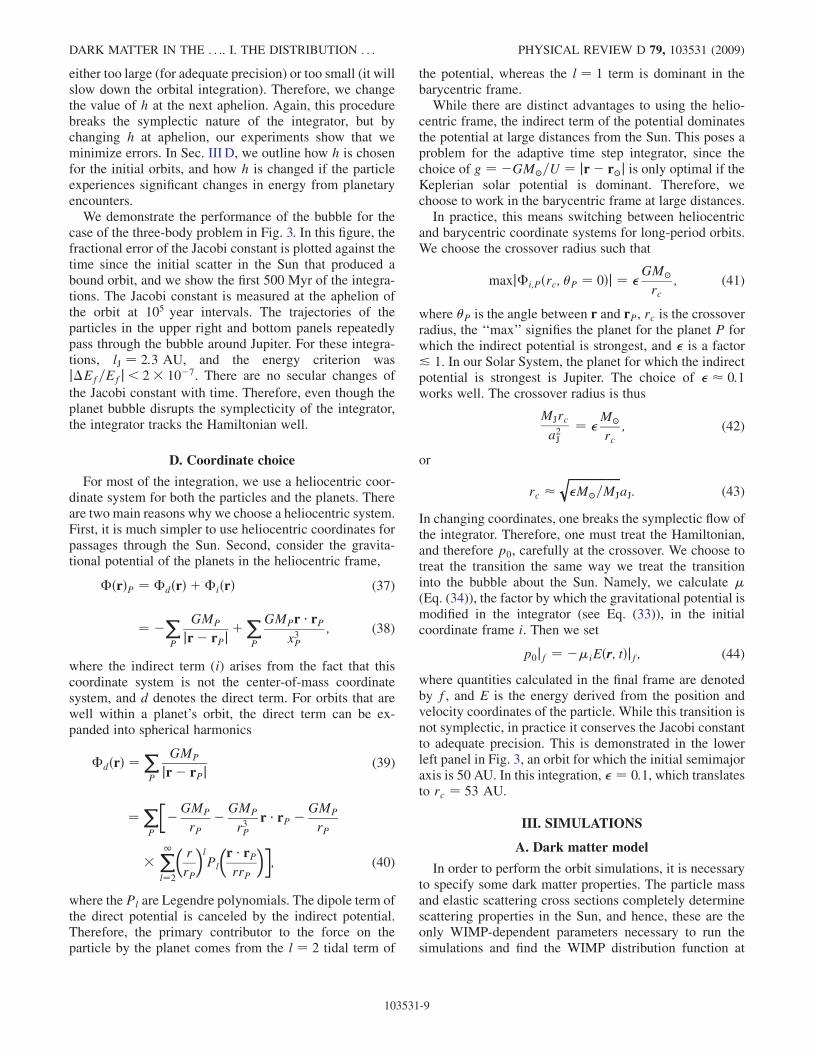
left panel of Fig. 3, where we show errors in the Jacobiconstant over a 500 Myr time span for an orbit with a �1:54 AU. The orbit enters the Sun� 107 times in this timespan. We sample the orbit at the first aphelion after a 105 yrinterval from the previous sample, and there are approxi-mately 100 steps/orbit. This figure shows that there areonly oscillatory errors throughout this long-term integra-tion, and these fractional errors never exceed 10�6 ataphelion. Long-term integrations of the two-body problemusing the map demonstrate energy errors only at the levelof machine precision.

2. The planets

While the adaptive time step integrator works well in anear-Keplerian potential, one must treat close encounterswith planets more carefully. If the time step is too largenear a planet, the particle fails to resolve the force from theplanet. This can cause growing errors in the particle’strajectory. Since we use an fðxÞ that is optimized to thepotential of the Sun, the only way to achieve a small timestep near each planet is to either make the fictitious timestep h small or to switch to a different integration methodnear each planet while using the method of Sec. II Awith areasonably large h for the rest of the orbit. The advantageof the former approach is that it does not break the sym-plectic nature of the integrator. However, it is also prohibi-tively computationally expensive. Therefore, we use thelatter approach.We define a spherical region (‘‘bubble’’) about each

planet for which we allow a different integration scheme,while continuing to use the adaptive time step symplecticintegrator (Sec. II A) outside the spheres. The transitionbetween the integration schemes is not symplectic, butreduces errors in the integration by enforcing an accuracyrequirement on j�E=Ej ¼ jðp0 þ EÞ=Ej ¼ jð�H þEÞ=Ej in the bubble of each planet.In the bubble of each planet, we continue to use the

adaptive time step integrator, but the value of h0 (the primedenotes the fact that this fictitious time step is only usedwithin a planet bubble) used in the bubble is selected tokeep the quantity j�E=Ej as small as possible while alsokeeping the total integration time short. To find the optimalvalue of h0, we use the following algorithm. When aparticle first enters a bubble, we record the particle’senergy error at the first step, j�Ei=Eij. Then, we integratethe particle’s trajectory through the bubble using the de-fault value of h. As the particle is about to exit the bubble,we calculate the energy error j�Ef=Efj. If the energy error


103531-7

meets the accuracy criterion, or if it is less than j�Ei=Eij,then the integration is allowed to continue normally. If,however, j�Ef=Efj does not satisfy the accuracy criterion,we restart the integration in the bubble from the point atwhich the particle first entered with a smaller fictitioustime step h0. This process iterates until either the energyaccuracy condition is satisfied or the energy error plateausin value. If the energy error plateaus in value, whichevertrajectory (corresponding to a particular choice of h0) hasthe minimum j�Ef=Efj is chosen.

The choice of the bubble size lJ is related to the choice offiducial value of h and to the mass of the planet. A largervalue of h means that the bubble needs to be larger to

ensure that the planet’s gravitational potential is properlyresolved. Planets with larger masses will require largerbubbles than smaller planets. We choose to keep the bubblesize fixed for all orbits. In general, we tune h so that thetypical energy errors for all energies are similar near eachplanet, and to keep the error in the Jacobi constant smallj�CJ=CJj< 10�4 at r ¼ 2R�. The optimum sizes of theJupiter bubble is l� 1–3 AU if we require thatj�Ef=Efj � 10�7–10�6.

A complication arises when particles experience largechanges in energy in their passage through the planetarybubble. In this case, the value of h that guaranteed a certainprecision in j�E=Ej in the pre-encounter orbit may be

FIG. 3 (color online). Error in the Jacobi constant as a function of time for several particles. The Jacobi constant is recorded ataphelion at 105 yr intervals. Top left: A particle with a ¼ 1:54 AU. This particle repeatedly goes through the Sun (about 107 times),but never goes through the bubble around Jupiter. It is integrated with h ¼ 6� 10�5R�1� yr, which corresponds to � 100 steps=orbit.Top right: A particle that gets stuck near a Sun-skimming 2:1 resonance with Jupiter. This particle repeatedly goes through the Jupiterbubble. It is integrated with h ¼ 2� 10�5R�1� yr, or � 350 steps=orbit. Bottom left: A particle gets stuck near a 3:2 resonance withJupiter. This orbit was integrated with h ¼ 1:5� 10�5R�1� yr, or� 650 steps=orbit. Bottom right: This particle repeatedly crosses rc,the transition radius between barycentric and heliocentric coordinates (dashed line marks rc=2, the crossing semimajor axis for an orbitwith e� 1) and has its last aphelion before ejection from the solar system at t ¼ 1:6� 106 years. It is integrated with h ¼2� 10�6R�1� yr, or 9� 103 steps=orbit.


103531-8

either too large (for adequate precision) or too small (it willslow down the orbital integration). Therefore, we changethe value of h at the next aphelion. Again, this procedurebreaks the symplectic nature of the integrator, but bychanging h at aphelion, our experiments show that weminimize errors. In Sec. III D, we outline how h is chosenfor the initial orbits, and how h is changed if the particleexperiences significant changes in energy from planetaryencounters.

We demonstrate the performance of the bubble for thecase of the three-body problem in Fig. 3. In this figure, thefractional error of the Jacobi constant is plotted against thetime since the initial scatter in the Sun that produced abound orbit, and we show the first 500 Myr of the integra-tions. The Jacobi constant is measured at the aphelion ofthe orbit at 105 year intervals. The trajectories of theparticles in the upper right and bottom panels repeatedlypass through the bubble around Jupiter. For these integra-tions, lJ ¼ 2:3 AU, and the energy criterion wasj�Ef=Efj< 2� 10�7. There are no secular changes of

the Jacobi constant with time. Therefore, even though theplanet bubble disrupts the symplecticity of the integrator,the integrator tracks the Hamiltonian well.

D. Coordinate choice

For most of the integration, we use a heliocentric coor-dinate system for both the particles and the planets. Thereare two main reasons why we choose a heliocentric system.First, it is much simpler to use heliocentric coordinates forpassages through the Sun. Second, consider the gravita-tional potential of the planets in the heliocentric frame,

�ðrÞP ¼ �dðrÞ þ�iðrÞ (37)

¼ �XP

GMP

jr� rPj þXP

GMPr rPx3P

; (38)

where the indirect term (i) arises from the fact that thiscoordinate system is not the center-of-mass coordinatesystem, and d denotes the direct term. For orbits that arewell within a planet’s orbit, the direct term can be ex-panded into spherical harmonics

�dðrÞ ¼XP

GMP

jr� rPj (39)

¼ XP

��GMP

rP�GMP

r3Pr rP �GMP

rP

� X1l¼2

�r

rP

�lPl

�r rPrrP

��; (40)

where the Pl are Legendre polynomials. The dipole term ofthe direct potential is canceled by the indirect potential.Therefore, the primary contributor to the force on theparticle by the planet comes from the l ¼ 2 tidal term of

the potential, whereas the l ¼ 1 term is dominant in thebarycentric frame.While there are distinct advantages to using the helio-

centric frame, the indirect term of the potential dominatesthe potential at large distances from the Sun. This poses aproblem for the adaptive time step integrator, since thechoice of g ¼ �GM�=U ¼ jr� r�j is only optimal if theKeplerian solar potential is dominant. Therefore, wechoose to work in the barycentric frame at large distances.In practice, this means switching between heliocentric

and barycentric coordinate systems for long-period orbits.We choose the crossover radius such that

maxj�i;Pðrc; �P ¼ 0Þj ¼ GM�rc

; (41)

where �P is the angle between r and rP, rc is the crossoverradius, the ‘‘max’’ signifies the planet for the planet P forwhich the indirect potential is strongest, and is a factor& 1. In our Solar System, the planet for which the indirectpotential is strongest is Jupiter. The choice of � 0:1works well. The crossover radius is thus

MJrca2J

¼ M�rc

; (42)

or

rc �ffiffiffiffiffiffiffiffiffiffiffiffiffiffiffiffiffiffiffiM�=MJ

qaJ: (43)

In changing coordinates, one breaks the symplectic flow ofthe integrator. Therefore, one must treat the Hamiltonian,and therefore p0, carefully at the crossover. We choose totreat the transition the same way we treat the transitioninto the bubble about the Sun. Namely, we calculate �(Eq. (34)), the factor by which the gravitational potential ismodified in the integrator (see Eq. (33)), in the initialcoordinate frame i. Then we set

p0jf ¼ ��iEðr; tÞjf; (44)

where quantities calculated in the final frame are denotedby f, and E is the energy derived from the position andvelocity coordinates of the particle. While this transition isnot symplectic, in practice it conserves the Jacobi constantto adequate precision. This is demonstrated in the lowerleft panel in Fig. 3, an orbit for which the initial semimajoraxis is 50 AU. In this integration, ¼ 0:1, which translatesto rc ¼ 53 AU.

III. SIMULATIONS

A. Dark matter model

In order to perform the orbit simulations, it is necessaryto specify some dark matter properties. The particle massand elastic scattering cross sections completely determinescattering properties in the Sun, and hence, these are theonly WIMP-dependent parameters necessary to run thesimulations and find the WIMP distribution function at


103531-9

the Earth. The particle physics model and parameter spacewithin each model do not need to be specified for thesimulations, although we assume that the dark matterparticle is a neutralino when we estimate event rates inneutrino telescopes in Sec. VI. Thus, we use m� to denote

the WIMP mass.The relative strengths of the spin-dependent and spin-

independent elastic scattering cross sections are importantin the context of scattering in both the Sun and the Earth.For simplicity in interpreting the simulations, we wouldlike to use either a spin-independent or spin-dependentcross section, but not a mixture of the two. We choose tofocus on the spin-independent cross section for the simu-lations, but in Sec. IVD, we show how to extend our resultsto the case of nonzero spin-dependent interactions. InSec. III D, we discuss the specific choices for the WIMPmass and �SI

p used in the simulations.

We adopt the Maxwellian distribution function

fhðx; vÞ ¼n�

ð2��2Þ e�v2=2�2

(45)

to describe the dark matter distribution function in the solarneighborhood in Galactocentric coordinates and far out-side the gravitational sphere of influence of the Sun. Here,� is the one-dimensional dark matter velocity dispersion,

set to � ¼ v�=ffiffiffi2

p. We set the speed of the Sun around the

Galactic center to be v� ¼ 220 km=s, for which the ob-servational uncertainty is about 10% [53,54]. The WIMPnumber density is n� ¼ �=m�. We assume that the dark

matter density is smooth and time-independent in theneighborhood of the Sun, and that � ¼ 0:3 GeV cm�3.

Even if the dark matter were somewhat lumpy, the resultsof the simulations will still be valid if � is interpreted as

the average density in the solar neighborhood [55].Transforming to the heliocentric frame via a velocity

transformation vs ¼ v� v�,

fsðx; vsÞd3xd3vs ¼ fhðx; vs þ v�Þd3xd3vs; (46)

where the subscript s refers to quantities measured in theheliocentric frame. This distribution is anisotropic withrespect to the plane of the Solar System (the ecliptic).The direction of the anisotropy with respect to the eclipticdepends on the phase of the Sun’s orbit about the Galacticcenter. In order to avoid choosing a specific direction forthe anisotropy (i.e., to avoid choosing to start our simula-tions at a particular phase of the Sun’s motion about theGalactic center), we angle-average this anisotropic distri-bution function to obtain an isotropic DF of the form

�fsðx; vsÞ ¼ 1

4�

Zfsðx; vsÞd� (47)

¼ 1

2ð2�Þ3=2n�

�v�vs

� ½e�ðvs�v�Þ2=2�2 � e�ðvsþv�Þ2=2�2�: (48)

Using the angle-averaged DF is approximately valid fortwo reasons: (i) Scattering in the Sun is isotropic, so anybound WIMPs produced by elastic scattering will initiallybe isotropically distributed. (ii) The time-averaged distri-bution function (averaged over the Sun’s � 200 Myr orbitabout the Galactic center) only has a small anisotropiccomponent [34], a consequence of the large (60) inclina-tion of the ecliptic pole with respect to the rotation axis ofthe Galaxy. If the flux at the Earth is dominated by particleswhose lifetime in the Solar System is greater than theperiod of the Sun’s motion about the Galactic center, theuse of time-averaged distribution function is appropriate.We use Liouville’s theorem to find the halo DF for an

arbitrary point in the Sun’s potential well. Neglecting thegravitational potential of the planets and the extremely rareinteractions between dark matter particles, each particle’senergy E is conserved:

E ¼ 1

2v2s (49)

¼ 1

2v2 þ��ðrÞ; (50)

where v is the speed of particle with respect to and in thegravitational sphere of influence of the Sun, and ��ðrÞ isthe gravitational potential of the Sun (�� ¼ �GM�=r forr > R�, where R� represents the surface of the Sun). Thus,the DF within the Sun’s potential well is

fðr; vÞ ¼ �fsðr; vsðr; vÞÞ; (51)

vsðr; vÞ ¼ffiffiffiffiffiffiffiffiffiffiffiffiffiffiffiffiffiffiffiffiffiffiffiffiffiffiffi2��ðrÞ þ v2

q: (52)

An important consequence of this result is that the distri-

bution function is identically zero for local velocities v <ffiffiffiffiffiffiffiffiffiffiffiffiffiffiffiffiffiffiffiffi�2��ðrÞp ¼ vescðrÞ below the escape velocity at thatdistance.

B. Astrophysics assumptions

The Sun: The Sun is modeled as spherical and nonrotat-ing. The gravitational potential and chemical compositionare described by the BS(OP) solar model [56]. We includethe elements 1H, 4He, 12C, 14Ni, 16O, 20Ne, 24Mg, 28Si, and56Fe in computing the elastic scattering rate.We treat the Sun with the ‘‘zero-temperature’’ approxi-

mation (i.e., the solar nuclei are at rest) since the kineticenergy of nuclei in the Sun is much less than the kineticenergy of dark matter particles. At the center of the Sun,the temperature is Tc � 107 K, so the average kineticenergy of a nucleus is of order

KA ¼ 3

2kTc (53)

� 1 keV: (54)


103531-10

In the cooler outer layers of the Sun, the nuclei have evenless kinetic energy. In contrast, the kinetic energy of darkmatter particles in the Sun is of order

K� �m�v2esc (55)

� 103�

m�

100 GeV

�keV: (56)

The rms velocity of the nuclear species A is hv2Ai1=2 ¼ffiffiffiffiffiffiffiffiffiffiffiffiffiffiffiffiffiffi

2KA=mA

p � 500ðmA=GeVÞ�1=2 km s�1, lower than the�103 km=s speed of dark matter particles. Therefore, togood approximation, one can treat the baryonic species inthe Sun as being at rest (i.e., having T ¼ 0)

The Solar System: The Solar System is modeled ashaving only one planet, Jupiter, since Jupiter has the largestmass of any planet by a factor of 3.3 and thereforedominates gravitational scattering. We place Jupiter on acircular orbit about the Sun, with a semimajor axis aJ ¼5:203 AU, its current value, for the entire simulation, sinceits eccentricity is only e � 0:05 [57], and the fractionalvariation in its semimajor axis is & 10�9 over the lifetimeof the Solar System [58]. Jupiter is modeled as havingconstant mass density to simplify calculations of particletrajectories. This is not a realistic representation ofJupiter’s actual mass density, but only a small fraction ofparticles scattered by Jupiter actually penetrate the planet.WIMP-baryon interactions in Jupiter are neglected sincethe optical depth of Jupiter is small enough that the proba-bility of even one scatter occurring in the simulation issignificantly less than unity.

The orbit of Jupiter defines the reference plane for thesimulation. The Earth’s orbit is assumed to be coplanarwith the reference plane, since the actual relative inclina-tion of the two orbits is currently only 1.3.

C. Initial conditions

The goal of this section is to compute the rate of elasticscattering of halo WIMPs by baryons in the Sun ontobound orbits, as a function of the energy and angularmomentum of particles after the scatter. We also showhow we use this to choose the initial starting positionsand velocities of the particles. There are two natural ap-proaches to this problem: (i) Sample the dark matter fluxthrough a shell a distance R> R� from the center of theSun, treating scatter in the Sun probabilistically, and keep-ing only those particles which scatter onto Earth-crossingbound orbits. (ii) Calculate the scattering probability in theSun directly. The second approach is more efficient, andthis is the one described below.

The initial energy of a dark matter particle is

E ¼ 1

2m�v

2 þ��ðrÞ (57)

¼ 1

2m�½v2 � v2

escðrÞ�; (58)

where we have expressed the gravitational potential interms of the local escape velocity from the Sun. The finalenergy of the dark matter particle is

E0 ¼ E�Q (59)

¼ 1

2m�½v02 � v2

escðrÞ�; (60)

where Q is the energy transfer between the dark matterparticle and the nucleus during the collision. The energytransfer can be expressed in terms of the center-of-massscattering angle � as (cf. Equation (A5))

Qðv; cos�Þ ¼ 2�2

A

mA

v2

�1� cos�

2

�; (61)

where

�A ¼ mAm�

mA þm�

(62)

is the reduced mass for a nuclear species of nucleonnumber A. The maximum energy transfer Qmax ¼2�2

Av2=mA occurs if the dark matter particle is back-

scattered, i.e., � ¼ �. Since we are interested in particlesthat scatter onto bound, Earth-crossing orbits,1 the inter-esting range of outgoing energy is

� GM�m�

2ð0:5a�Þ � E0 � 0; (63)

where a� is the semimajor axis of the Earth’s orbit, withthe lower bound determined by the fact that the aphelion ofa highly eccentric orbit is 2a.For a given incoming energy E, it may not be kinemati-

cally possible to scatter into the full range of bound, Earth-crossing orbits. In particular, if E�Qmax ¼ E0

min > 0, theparticle cannot scatter onto a bound orbit at all. Therefore,the lower bound on allowed outgoing energy is

E0min ¼ max

��GM�m�

2ð0:5a�Þ ;minðE�QmaxðvÞ; 0Þ�; (64)

while the upper bound remains

E0max ¼ 0: (65)

Thus scattering rate of particles onto bound, Earth-crossingorbits is

d _N�drd�rdvdQ

¼ 4�XA

r2nAðrÞv3 d�A

dQfðr; vÞ�ðR� � rÞ

��½�E0��½E0 � E0min�; (66)

1In principle, particles scattered to bound orbits with a < a�=2could later evolve onto Earth-crossing orbits. However, thetorque from Jupiter is never high enough to pull a particlewith a < a�=2 onto an Earth-crossing orbit unless ðða�=2Þ �aÞ=a & 10�3. Moreover, each additional scatter in the Sunreduces the energy of the orbit in the limit of a cold Sun, sothe semimajor axis may only shrink.


103531-11

where we have imposed spherical symmetry on the Sun,�r is the solid angle in the Sun, fðx; vÞ is the distributionfunction in Eq. (51), d�A=dQ is the WIMP-nucleus crosssection (Eq. (A1)), and �ðxÞ is the step function. Since

dE0 ¼ dQ; (67)

we can write Eq. (66) as

d _N�drd�rdvdE

0 ¼ 4�XA

r2nAðrÞv3 d�A

dQfðr; vÞ�ðR� � rÞ

��½�E0��½E0 � E0min�: (68)

By sampling this distribution, we find the initial energy,speed, and scattering position vector of the WIMPs.

The outgoing energy is distributed uniformly unlessthere is kinematic suppression. The kinematic suppressionis most pronounced for large WIMP masses and verynegative energies because, in order for a particle to scatteronto a bound orbit,

vs � 2

ffiffiffiffiffiffiffiffiffiffiffiffiffim�mA

pm� �mA

vescðrÞ (69)

where vs is the particle velocity at infinity. Heavy darkmatter particles can only scatter onto bound orbits if theirvelocities at infinity are only a small fraction of the escapevelocity from the Sun, a distance r from the Sun. Forenergies for which the kinematic suppression is minimal,we express the uniformity of d _N�=dE0 in terms of thesemimajor axis. Since E0 ¼ �GM�=2a for particles onelliptical orbits, d _N�=da / a�2, or

d log _N�d loga

¼ �1: (70)

Therefore, most particles scatter onto relatively smallorbits.

The angular momentum of each scattered particle is inthe range J 2 ½0; rv0�, where r is the radius from the centerof the Sun at which the particle scatters. To determine thedistribution of magnitudes and directions for the angularmomentum, we assume that the direction of the finalvelocity v0 is isotropically distributed with respect to theposition vector r. If we specify �v to be the colatitude ofthe velocity vector with respect to the position vector, andthe magnitude of the angular momentum is J ¼ rv0 sin�v,then the distribution in angular momentum at fixed r, v0 hasthe form

d _N� / d cos�v ¼ dJ2

2r2v02 ffiffiffiffiffiffiffiffiffiffiffiffiffiffiffiffiffiffiffiffiffiffiffiffiffiffiffiffiffiffi1� J2=ðr2v02Þp : (71)

The effect of kinematic suppression due to a large WIMPmass is that the particles that do scatter onto bound orbitscan only do so close to the center of the Sun where vesc ishighest. This reduces the maximum angular momentum of

the outgoing particle, and so eccentricity is an increasingfunction of WIMP mass.By sampling Eqs. (68) and (71), and the azimuth of v0

with respect to the position vector, we fully specify the six-dimensional initial conditions of the WIMPs, sampled tothe same density as they would actually scatter in the Sun.

D. Simulation specifics

The goals of the simulations are to predict the direct andindirect detection signals from particles bound to the SolarSystem (relative to the signal from unbound particles) as afunction of m� and the elastic scattering cross section. We

simulate orbits for a variety of WIMP parameters and theninterpolate the results for other values of those parameters.We ran four sets of simulations with different choices of

m� and �SIp . The first simulation, called ‘‘DAMA,’’ used

m� ¼ 60 atomic mass units (AMUs) and �SIp ¼

10�41 cm2. These parameters lie in the DAMA annualmodulation region [59,60]. A second simulation, called‘‘CDMS,’’ used the same WIMP mass as in the DAMAsimulation but a cross section 2 orders of magnitude lower,�SI

p ¼ 10�43 cm2, below the minimum of the CDMS 2006

exclusion curve (Fig. 4). Two more simulations werechosen to have �SI

p ¼ 10�43 cm2 but with larger WIMP

masses. The ‘‘Medium Mass’’ simulation uses m� ¼150 AMU, and the ‘‘Large Mass’’ simulation uses m� ¼500 AMU, selected to explore the dependence of thesimulations on WIMP mass. The choices for m� and �SI

p

are plotted in Fig. 4 in addition to some recent directdetection results. The details on the initial conditions ofthe simulations are summarized in Table I.Since integrating the orbits of particles in the Solar

System is computationally expensive, it is more importantto integrate just enough orbits to determine the approxi-mate size of the bound DF relative to the unbound distri-bution, and to get a sense of which effects matter the most,than it is to get small error bars on the DF. This principleguides our choices in the sizes of the ensembles ofparticles.The number of particles simulated Np in each of the

solar capture simulations is given in Table I. We followparticles with semimajor axes slightly below the Earth-crossing threshold so that if the semimajor axis increasesmodestly during the simulation, the contribution to theEarth-crossing flux is included. Fewer particles were simu-lated in the runs with a lower cross section because thelifetimes were far longer than in the DAMA run.We use the flowchart in Fig. 5 to sketch the simulation

algorithm. There are six things that need to be set in orderto run the simulations: starting conditions; the radius rc atwhich the heliocentric-barycentric coordinate changeneeds to be made; methods for initializing h and poten-tially changing h at later times; conditions for passingthrough and scattering in the Sun; the size of the bubble


103531-12

about Jupiter, lJ, and the accuracy criterion j�E=Ej; andconditions for terminating the simulation. Following theflowchart, we discuss each point in turn.

Starting Conditions We sample the distribution ofWIMPs initially scattered into the Solar System accordingto Eqs. (68) and (71). Once we have determined the initialposition and velocity of each WIMP, we trace the WIMPsback to perihelion and start the integration there. We followall particles after the initial scatter, using the map to evolvethe particles to the Sun bubble wall (0.1 AU) using the mapdescribed in Sec. II C 1. In order to account for the fact thatparticles may experience a second scatter before leavingthe Sun for the first time, we perform a rescatteringMonte Carlo when we construct the DFs.

Once the particles have reached the bubble boundary, weinitialize the adaptive time step symplectic integrator

(Sec. II A), setting h ¼ 10�8R�1� yr and integrating theequations of motion in heliocentric coordinates. With thischoice of initial h, a particle with initial semimajor axisa ¼ 1 AU will be integrated with 4:7� 105 steps=orbit,while a particle with a ¼ 100 AU will be integrated with4:7� 106 steps=orbit. We choose such a small h to mini-mize errors near perihelion, which is the point in the orbitat which errors are largest (Sec. II B). If the semimajor axisexceeds rc=2, it may be necessary to change to barycentriccoordinates before the particle reaches aphelion for the firsttime.Coordinate Change For the weak scattering simulations,

we set ¼ 0:1 (Eq. (41)), thus setting the transition radiusbetween the heliocentric and barycentric coordinated re-gimes to rc ¼ 53 AU. This is large enough that only asmall percentage of particles routinely cross the transitionradius, but small enough that the heliocentric potentialdoes not have too large a contribution from the indirectpotential.Setting h: After the particles reach their first aphelion,

h is reset according the values listed in Table II.These values of h are chosen such that both errors atperihelion (j�E=Ej< 10�4) and near Jupiter (j�E=Ej<10�6) are small. The combination of the values of h andthe Jupiter bubble radius lJ (see below) were determinedempirically. We used slightly smaller values of h forsome semimajor axes in the CDMS, Medium Mass,and Large Mass runs compared to the DAMA run inorder to check that the behavior of long-lived WIMPswas not an artifact of the choice of parameters.A particle’s energy (and hence, semimajor axis) may

change throughout the simulation. If the energy changes by20% or more from when the particle enters the Jupiterbubble to when it exits, the particle is flagged to have hadjusted at the next aphelion. We do not readjust h afterevery aphelion, or after each time the particle passesthrough the bubble, because very frequent changes in hcan induce growing numerical errors in the Jacobi con-stant. We impose any changes in h at aphelion instead ofthe bubble boundary, since we have determined experi-mentally that the aphelion is the optimal point at which tochange h.The Sun Bubble When a particle first crosses into the

bubble about the Sun, we calculate its perihelion. If theperihelion is smaller than 2R�, we proceed to map itscurrent position and velocity to its position and velocityas it exits the bubble according to the prescription ofSec. II C 1. If the perihelion lies within the Sun, we employa Monte Carlo simulation of scattering in the Sun(Appendix B). The vast majority of the time, the particledoes not scatter, and we simply use the map to move theparticle to the edge of the bubble. If the particle rescattersonto an orbit with semimajor axis a < 0:3 AU, we termi-nate the integration. If the particle rescatters onto an orbitwith a > 0:3 AU, we evolve the new orbit to the edge of

WIMP Mass [GeV/c2]

Cro

ss-s

ectio

n [c

m2 ]

(nor

mal

ised

to n

ucle

on)

080707150400

http://dmtools.brown.edu/ Gaitskell,Mandic,Filippini

101

102

103

10-46

10-44

10-42

10-40

DAMA

MedMass

LargeMassCDMS

080707150400XENON1T (projected, 1 ton-year exposure)SuperCDMS (Projected) 25kg (7-ST@Snolab)XENON10 2007 (Net 136 kg-d)CDMS: 2004+2005 (reanalysis) +2008 GeCDMS (Soudan) 2004 + 2005 Ge (7 keV threshold)DAMA 2000 58k kg-days NaI Ann. Mod. 3sigma w/DAMA 1996DATA listed top to bottom on plot

FIG. 4 (color online). Points in the �SIp �m� parameter space

used for the solar capture simulations, plotted along with exclu-sion curves from recent experiments. This plot was generatedwith http://dendera.berkeley.edu/plotter/entryform.html.

TABLE I. Solar capture simulations.

Name m� [AMU] �SIp [cm2] Np [a > 0:48 AU]

DAMA 60 10�41 1078586

CDMS 60 10�43 145223

Medium Mass 150 10�43 144145

Large Mass 500 10�43 148173


103531-13

the bubble, and then resume the adaptive time step sym-plectic integration.

The Jupiter Bubble For the DAMA, CDMS, andMedium Mass simulations, we set the Jupiter bubbleboundary to be lJ ¼ 1:7 AU, and the accuracy criterion

to be j�Ef=Efj< 10�6. We adjusted this value for some

particles in order to speed up the integration in cases whereparticles had generically slightly smaller initial j�Ei=Eijthan j�Ef=Efj, and took a longer time with j�Ef=Efj ¼10�6 to reach a sufficiently flat plateau in j�Ef=Efj than

Solar Capture Simulations

adaptive timestep integratorheliocentric coordinates

fiducial h

Cross rc fromabove?

No

Yes

fiducial hbarycentric coordinates

adaptive timestep integrator

Cross rc fromabove?

No

First apocenter?

First apocenter?

No

Yes

Yeschange fiducial h

No

In planetbubble?

Yes

adaptive timestep integratorheliocentric coordinates

optimal h’

a>0.3 AU?

Scatter?

Use map

No

r > 2R ?o

Yes

In Sunbubble?

Yes

Does p_0 changeby > 20%?

END

No

Yes

No

No

Yes

No

Use map to r=0.1 AUh = 10^−8 R_0^−1 year

Yes

Yes

STARTr = r_p

Yes

No

change fiducial h

Yes

No

r > 5000 AU?

change fiducial h

END

FIG. 5. Flowchart for the simulation algorithm for the solar capture experiments.


103531-14

with a slightly larger accuracy criterion. We set lJ ¼3:4 AU past 500 Myr for the Medium Mass simulation todetermine if there were any effects of a larger lJ on theorbits. There were no effects on the DF resulting from thischange. For the Large Mass simulation, we experimentedwith a lower value of the accuracy criterion (j�Ef=Efj<2� 10�7 for the first 500 Myr, j�Ef=Efj< 3� 10�7

later) and a larger bubble, lJ ¼ 2:1 AU. The only effectthe larger accuracy criterion had was to raise slightly themaximum energy error per orbit.

Stopping Conditions There are three reasons for termi-nating an integration. If the particle crosses outwardthrough the shell r ¼ 5000 AU, the integration stops.Particles crossing this shell will rarely cross the Earth’sorbit again. Second, if the particle rescatters in the Sunonto an orbit with a < 0:3 AU, we halt the integrationsince the particle will soon thermalize in the Sun andwill not cross the Earth’s orbit. Third, we stop the integra-tion if the particle survives for a time t� ¼ 4:5 Gyr, ap-proximately the lifetime of the Solar System.

E. Computing

Simulations were performed on three Linux beowulfcomputing clusters at Princeton University. Each set ofsimulations required 105 CPU cycles on 3 GHz dual coreprocessors.

IV. DISTRIBUTION FUNCTIONS

Before presenting the results of the simulations, wedefine some terms that will be used frequently in thissection. The ‘‘heliocentric frame’’ describes an inertialframe moving with the Sun. ‘‘Heliocentric speeds’’ willrefer to speeds relative to the Sun, measured at the Earth

assuming the Earth has zero mass. The ‘‘geocentric frame’’refers to an inertial frame moving with the Earth. Unlessotherwise noted, geocentric WIMP speeds are those out-side the potential well of the Earth. The ‘‘free space’’distribution function, Eq. (48), is the angle-averaged halodistribution function in an inertial frame moving with theSun, outside of the gravitational sphere of influence of theSun. The ‘‘unbound’’ distribution function refers to theLiouville transformation of the free space distributionfunction to the position of the Earth (Eq. (51)), includingthe effects of the gravitational field of the Sun but not theEarth.In Fig. 6, we present the one-dimensional geocentric

DFs divided by the haloWIMP number density n� (defined

in Sec. III A) for each simulation. These DFs have alreadybeen integrated over angles, and are normalized such thatthe bound dark matter density n�;bound ¼

Rdvv2fðvÞ,

where fðvÞ ¼ Rd�fðvÞ. We plot the DFs in Fig. 6(a) on

a logarithmic scale in order to highlight the structures,while we plot the CDMS simulation (Table I) DF on alinear scale in Fig. 6(b) to compare the simulation resultswith theoretical DFs. The DFs are based on ð1–4Þ � 108

passages of particles within a height jzj< zc ¼ 10R� ofthe Earth’s orbit, and estimated using the technique de-scribed in Appendix C. The DFs are insensitive to zc, atleast in the range 1 & zc & 25R�. Error bars are based on500 bootstrap resamplings of the initial scattered particledistributions for each simulation.The most striking feature of the DFs is the smallness

with respect to the DF of haloWIMPs unbound to the SolarSystem. This is in stark contrast to the prediction ofDamour and Krauss [37]. In order to show why this isthe case, we examine the simulations in detail. In particu-lar, we (i) identify the features in the DF with specific typesof orbits, (ii) find the lifetime distribution of such orbits,and (iii) determine what sets the lifetime of those orbits(e.g., ejection vs rescattering and thermalization in theSun). With these data, we may also determine how theDF varies with WIMP mass and cross section, and estimatethe maximum DF consistent with limits on the spin-independent cross section.The DFs from the four simulations show similar mor-

phologies, although the normalization of the features dif-fers. The most prominent feature in all four DFs in Fig. 6 isthe ‘‘high plateau’’ between 27< v< 48 km s�1. Inorder to identify which orbits contribute to this plateau,it is useful to examine the two-dimensional DF. In Fig. 7,we show the two-dimensional DF fðv; cos�Þ ¼Rd�fðv; cos�;�Þ for the CDMS simulation (Table I) in

both (a) heliocentric and (b) geocentric coordinates. Theangle between the velocity vector and the direction of theEarth’s motion is �, while � is an azimuthal angle, with� ¼ 0 corresponding to the direction of the north eclipticpole if � ¼ �=2. The DFs are plotted on a logarithmicscale to highlight structure. We only show the CDMS

TABLE II. The fictitious time step h as a function of semi-major axis a for the DAMA simulation and the simulations with�SI

p ¼ 10�43 cm2 (CDMS, Medium Mass, Large Mass).

a [AU]

DAMA

h [R�1� yr]�SI

p ¼ 10�43 cm2 h[R�1� yr]

a < 0:75 1� 10�4 1� 10�4

0:75 � a < 1:1 7� 10�5 7� 10�5

1:1 � a < 1:6 6� 10�5 6� 10�5

1:6 � a < 2:2 5� 10�5 2� 10�5

2:2 � a < 3:5 4� 10�5 2� 10�5

3:5 � a < 6:2 3� 10�5 1:5� 10�5

6:2 � a < 11 2� 10�5 1� 10�5

11 � a < 13 9� 10�6 2� 10�6

13 � a < 22 2� 10�6 2� 10�6

22 � a < 30 2� 10�6 2� 10�6

30 � a < 45 1� 10�6 1� 10�6

45 � a < 120 6� 10�7 6� 10�7

120 � a < 200 4� 10�7 4� 10�7

200 � a < 500 3� 10�7 3� 10�7

a > 500 or unbound 2� 10�7 2� 10�7


103531-15

simulation results in this figure since the phase spacestructure of the DF is virtually the same in all simulations.

From Fig. 7(b), we identify the short arc between 27<v< 50 km s�1 below cos� <�0:5 with the high plateau,although there is a small contribution from the other,longer arc. We find that the short arc in the geocentricDF corresponds to the trumpet-shaped feature in the helio-centric DF below v < 38 km s�1. For bound orbits, theheliocentric speed at r ¼ 1 AU is

vðaÞ ¼�2�

�a

a�

��1�1=2

v�; (72)

where v� is the orbital speed of the Earth. The heliocentricspeed v ¼ 38 km s�1 corresponds to the lowest Jupiter-

crossing orbit, so the trumpet feature in the two-dimensional heliocentric DF corresponds to orbits that donot cross Jupiter’s orbit.The trumpet shape of the heliocentric DF (and the

narrow band in the geocentric DF) in Fig. 7 can be simplyexplained. In Fig. 8, we calculate the energy and angularmomentum for each point in velocity-space. The blackregion of velocity-space represents unbound orbits. Allpoints for which orbits are bound and have perihelia insidethe Sun are marked in dark grey, while orbits that are boundand cross Jupiter’s orbit are marked in light grey. The whiteregions correspond to bound orbits that neither enter theSun nor cross Jupiter’s path. If we were to integrate the�-slices shown if Fig. 8, we would find that the region in

FIG. 7 (color online). Distribution functions divided by n� in the v� cos� plane (integrated over �) for both (a) heliocentric and(b) geocentric frames. These DFs come from the CDMS simulation, and the units are ðkm s�1Þ�3.

(a) (b)

10-15

10-14

10-13

10-12

10-11

10-10

10-9

10-8

0 10 20 30 40 50 60 70

f(v)

/ n χ

[(km

/s)-3

]

v [km/s]

DAMACDMS

Med MassLarge Mass

0

1

2

3

4

5

6

7

8

0 10 20 30 40 50 60 70

f(v)

/ n χ

[10-8

(km

/s)-3

]

v [km/s]

Geocentric DF, mχ = 60 AMU, σpSI = 10-43 cm2

Free spaceUnbound

CDMS

FIG. 6 (color online). Geocentric distribution functions from the simulations. (a) Results from all simulations. (b) The CDMSdistribution function relative to theoretical distribution functions for unbound WIMPs.


103531-16

Fig. 8 corresponding to Sun-penetrating orbits that do notcross Jupiter exactly matches the parts of phase space weidentified with the high plateau.

Figure 8 was computed for a system without planets.Once Jupiter is added, another type of orbit that may existis a bound orbit for which Jz is fixed but J is not. Anexample of this type of orbit is a Kozai cycle. In this case,Jz ¼ a�v cos� in the heliocentric frame. In the specialcase that � ¼ �=2, J ¼ Jz. Therefore, the parts ofðv; cos�Þ phase space in the� ¼ �=2 plane correspondingto Sun-penetrating orbits also cover orbits with Jz fixed bythe initial scatter in the Sun for other values of�. Thus, thehigh plateau in the one-dimensional geocentric DF is builtup by WIMPs with a < aJ=2 and small Jz but not neces-sarily small J.

The second feature of the distribution functions in Fig. 6is the ‘‘low plateau.’’ This is the relatively flat part of thedistribution function that extends from � 10 km s�1 to �70 km s�1. This feature corresponds in the long arc in thetwo-dimension DF in Fig. 7 and the stripe between 38<v< 42 km s�1 in the heliocentric DF. From Fig. 8, weidentify this feature with bound, Jupiter-crossing orbits.

Small gaps exist in the heliocentric DF with v >40 km s�1 and cos� < 0 and 38< v< 40 km s�1 andcos� > 0 because these regions of phase space are inac-cessible to WIMPs initially scattered in the Sun in therestricted three-body problem. This translates to a trunca-tion of the low plateau at the extrema in geocentric speed.The third common set of features in the one-dimensional

geocentric distribution function are spikes in the low pla-teau. These spikes result from the long-lifetime tail ofJupiter-crossing or nearly Jupiter-crossing particles thatspend significant time near mean-motion resonances oron Kozai cycles. The minimum semimajor axis for thesespikes corresponds to the 3:1 resonance, a � 2:5 AU.Long-lifetime tails due to ‘‘resonance-sticking’’ orbitshave also been observed in simulations of comets[61,62]. The error bars on the spikes are large due to thesmall numbers of long-lived resonance-sticking particles ineach simulation. There is also some Poisson noise in theheight of the spikes between simulations due to the smallnumber long-lived WIMPs in each simulation.Next, we show the lifetime distribution of boundWIMPs

and demonstrate which mechanisms (thermalization or

FIG. 8. Locations of various types of orbits in the (a) � ¼ 0 and (b) � ¼ �=2 slices of heliocentric velocity-space, and (c) � ¼ 0and (d) � ¼ �=2 slices of geocentric velocity-space.


103531-17

ejection) terminate the contribution of orbits to the DF. InFig. 9, we present the lifetime distributions for all WIMPsin the DAMA, CDMS, Medium Mass and Large Masssimulations. There are several notable features in thisplot. First, and most striking, many of the bound particlessurvive for very long times—up to 106–108 yr. However,in none of the simulations is there a large population ofparticles that survive for times of order of the age of theSolar System, although there is a small population thatdoes (the notch at 4.5 Gyr in Fig. 9). Second, the lifetimedistribution functions of the CDMS, Medium Mass, andLarge Mass runs are very similar. However, these lifetimedistributions are quite different from that of the DAMAsimulation. The differences in the lifetime distributions aredue almost entirely to the elastic scattering cross section, atleast for the range of WIMP masses we consider.

In order to both explain these features in the lifetime andphase space distribution functions, it is useful to examinethe lifetime distributions as a function of the initial semi-major axis ai, as shown in Fig. 10.

The largest feature in Fig. 9 is the strong peak at tl �103 yr for the DAMA simulation and tl � 105 yr for thesimulations with �SI

p ¼ 10�43 cm2, which we call the ‘‘re-

scattering peak.’’ It encompasses the majority of particlesin each simulation. This feature results from WIMPs thatrescatter in the Sun before they are ejected from the SolarSystem by Jupiter or precess onto orbits that do not inter-sect the Sun. This rescattering peak is offset betweenDAMA and the other simulations because the lifetime isinversely proportional to the scattering probability in theSun, tl / ��1

p .

There is one important difference in the composition ofthe rescattering peak between the DAMA and other simu-lations. In Fig. 10, we show that particles on Jupiter-crossing orbits exhibit a rescattering feature in theDAMA simulation but not in the other simulations.Indeed, about 23% of Jupiter-crossing particles in theDAMA simulation are rescattered in the Sun, while <2%are rescattered in the other simulations. This is because thetime scale on which Jupiter can perturb the perihelia ofJupiter-crossing orbits out of the Sun is significantlyshorter than rescattering time scales for the �SI

p ¼10�43 cm2 simulations, but the two time scales becomecloser at higher cross sections.Another feature occurs at tl � 106 yr, which we call the

‘‘ejection peak.’’ This feature occurs at the same time foreach simulation, and from Fig. 10 we see that this arisesfrom Jupiter-crossing orbits. The median time at which thisfeature occurs is independent of �SI

p since ejection, not

rescattering, sets the lifetime of these WIMPs. The slope ofthe Jupiter-crossing lifetime distribution changes near�10 Myr for all simulations. WIMPs that have tl >10 Myr are resonance-sticking, and their lifetime distribu-tion goes as NðtÞ / t��, where � is slightly less than one.A third feature, called the ‘‘quasi-Kozai peak,’’ is cen-

tered at tl � 106 yr in the DAMA simulation, and tl �108 yr in the other simulations. The feature is seen in the1:5 AU � ai < 2 AU and 2 AU � ai < aJ=2 bins ofFig. 10. The WIMPs in the quasi-Kozai peak are not ontrue Kozai cycles because of significant interactions withmean-motion resonances. In the simulations, particles inthe quasi-Kozai peak are observed to alternate betweenrescattering peak-type orbits with perihelion well insidethe Sun, and orbits that look like Kozai cycles. Both thesemimajor axis and Jz vary with time; neither is conservedalthough the combination giving the Jacobi constant CJ isfixed (Eq. (20)). There are some orbits at the low end of thesemimajor axis range 1:5 AU< a � aJ=2 for which a andJz are conserved and the Kozai description is accurate.The median lifetime of WIMPs on quasi-Kozai cycles is

well described by tl=P� � 300=�, where P� is the WIMP

orbital period and � is the optical depth through the centerof the Sun. This implies that particles are eventually re-moved from Earth-crossing orbits by rescattering in theSun. The height of the rescattering peak relative to thequasi-Kozai peak is greater in the DAMA simulation thanthe other simulations because the optical depth in the Sunis large enough that particles originating deep within theSun rescatter before the torque from Jupiter can pull theperihelion towards the surface of the Sun.The fourth feature is not obvious in Fig. 9, but is once the

lifetime distribution is displayed on logarithmic scales inFig. 10. This feature is the ‘‘Kozai peak.’’ This peak islocated at about tl � 108 yr for the DAMA simulation, andnear tl � t� ¼ 4:5 Gyr for the other simulations. Thisfeature results from particles whose orbital evolution can

FIG. 9 (color online). Particle lifetime distributions for theDAMA (solid), CDMS (dot-dashes), Medium Mass (shortdashes), and Large Mass (long dashes) simulations.


103531-18

be described by Kozai cycles (a, Jz conserved), of whichwe see both circulating and librating populations. For theCDMS, Medium Mass, and Large Mass simulations, thepeak is at t� because that is the time at which we terminatethe simulations. Particles on these orbits have ai <1:5 AU, and originate in the outer r * 0:5R� in the Sun.They constitute only a small fraction (� 0:1%) of all orbitswith ai < 1:5 AU, but dominate the lifetime distribution ofparticles with lifetimes * 108 yr. The median lifetime ofparticles on Kozai cycles depends on the WIMP-nucleoncross section in the form tl=P� � 105=�, where again � is

the optical depth through the very center of the Sun (��10�3 for DAMA, �� 10�5 for the other simulations).Now that we have identified the types and lifetimes of

bound WIMP orbits, we see how these come together tobuild up the phase space DF as a function of WIMP massand cross section.

A. The distribution function as a function of �SIp

We have identified (i) which range of initial semimajoraxis ai corresponds to the features in the geocentric DFs inFig. 6, and (ii) described the lifetime distributions of

FIG. 10 (color online). Lifetime distributions as a function of initial semimajor axis.


103531-19

WIMPs. Next, we describe the composition (not just interms of the semimajor axis ai but by the type of orbit) andheight of the DFs as a function of �SI

p . This is most easily

illustrated with the time-evolution of the DFs, which weshow in Fig. 11 for the (a) DAMA and (b) CDMS simula-tions. We focus on these two simulations since the salientresults of the Medium Mass and Large Mass simulationsclosely resemble those of the CDMS run. In each plot, weshow distribution functions as a function of time since thebirth of the Solar System, for t ¼ 106 yr, t ¼ 107 yr, t ¼108 yr, t ¼ 109 yr, and t ¼ t� ¼ 4:5 Gyr.

The low plateau, composed of Jupiter-crossing particles,has reached equilibrium in both �107 year for both simu-lations. The only growth in the low plateau after 10 Myrcomes from particles on resonance-sticking orbits thatpump up the spikes. The time-evolution of the low plateau(but not its final equilibrium height) is independent of crosssection over 2 orders of magnitude in the WIMP-baryoncross section because the equilibrium time scale is essen-tially the ejection timescale. The height of the low plateauis proportional to the rate at which particles are initiallyscattered onto Jupiter-crossing orbits, _NJ. Since the scat-tering rate is proportional to the cross section, the height ofthe low plateau is proportional to the spin-independentcross section, at least in these simulations. One wouldexpect that the plateau height would grow less rapidlywith �SI

p if the lifetimes of Jupiter-crossing WIMPs were

dominated by rescattering in the Sun, not ejection from theSolar System.

The absolute height of the spikes is similarly related to_NJ and the relative ejection and rescattering time scales;the spikes in the DAMA simulation are more prominentthan in the CDMS simulation because _NJ is 2 orders ofmagnitude larger. The time-evolution of the spikes can beexplained by the following. The lifetime distribution ofspike WIMPs falls as NðtÞ / t��, where � is slightly lessthan one. The rate at which WIMPs cross the Earth’s orbitis _NcðtÞ ¼ const if the long-lived WIMPs are resonance-sticking. Therefore, the total contribution of the spikeWIMPs to the DF beyond time t goes as

fspikeð>tÞ /Z t�

tNðt0Þ _Ncðt0Þdt0 (73)

/ t1�� t1��: (74)

This argument is only strictly true if the types of spikeorbits are independent of the lifetime distribution, which isuncertain due to the small number statistics of the spikeWIMPs. However, in Fig. 11, some of the spikes eithergrow linearly with time or do not grow at all for somestretches of time. This phenomenon is due to the smallnumbers of long-lived resonance-sticking particles. For anindividual WIMP, fðvÞ / t if t < tl and fðvÞ is fixed fort > tl.

The time-evolution of the high plateau is different be-tween the DAMA and CDMS simulations. In the DAMAsimulation, by t ¼ 1 Myr, nearly all of the rescatteringpeak WIMPs have rescattered and thermalized in theSun, as have a significant fraction of the quasi-KozaiWIMPs. At this point, the high plateau in the range27 km s�1 < v< 45 km s�1 is built up by roughly similarcontributions from rescattering and Kozai peak WIMPs.The contribution of Kozai WIMPs relative to rescatteringpeak WIMPs at a particular time can be estimated using

fKozaifrescatt

� �

�t

tmed

�; (75)

where fKozai is the DF due to Kozai cycling WIMPs, frescattthat of rescattering peak WIMPs, � is the fraction ofWIMPs with a < 1:5 AU on Kozai cycles, and tmed is themedian lifetime of rescattering peak WIMPs. � � 10�3

(a)

10-14

10-13

10-12

10-11

10-10

10-9

10-8

0 10 20 30 40 50 60 70

f(v)

/nχ

[(km

/s)-3

]

v [km/s]

t = 106 yrst = 107 yrst = 108 yrst = 109 yrs

Total

(b)

10-14

10-13

10-12

10-11

10-10

10-9

10-8

0 10 20 30 40 50 60 70

f(v)

/nχ

[(km

/s)-3

]

v [km/s]

t = 106 yrst = 107 yrst = 108 yrst = 109 yrs

Total

FIG. 11 (color online). Growth of the distribution functions asa function of time for the (a) DAMA and (b) CDMS simulations.


103531-20

for WIMPs experiencing Kozai cycles, and tmed � 103 yr,so fKozai=frescatt � 1 at t ¼ 1 Myr. This assumes that theincrease in the DF for a Kozai cycling WIMP as a functionof time is similar to that of a WIMP on a rescattering peak-type orbit. The feature in the DF between 45 km s�1 <v< 50 km s�1 is due to quasi-Kozai WIMPs.

The high plateau grows substantially between t ¼1 Myr and t ¼ 100 Myr, although not strictly linearlybecause scatters in the Sun remove Kozai and quasi-Kozai WIMPs from Earth-crossing orbits. The error barson the DF increase with time as the ever-decreasing num-ber of Earth-crossing WIMPs (Fig. 10) build up the DF.After 100 Myr, the high plateau grows very slowly until itreaches equilibrium by t ¼ 1 Gyr; in our simulation of 8�105 WIMPs with orbits interior to Jupiter’s orbit, only oneWIMP has a lifetime of 1 Gyr.

Even though we simulate�103 WIMPs on Kozai cycles,we are clearly undersampling those with tl > 109 yr. Toestimate how much larger the DF could be, we note that thelifetime distribution of Kozai WIMPs with tl > 100 Myr iswell fit by NðtÞ / t�2. If we assume that the rate at whichthe long-lived WIMPs contribute to the DF as a function oftime is the same as for the Kozai WIMPs we simulate, then_NcðtÞ ¼ const. Therefore, according to Eq. (73), the part ofthe DF built after time t is fKozaiðv;>tÞ / t�1. For the highplateau, fKozaiðv; t > 108 yrÞ � fKozaiðv; t > 109 yrÞ, sowe believe that we have not underestimated the highplateau.

A major consequence of this equilibrium distribution isthat the high plateau of the DF fðvÞ=n� is fixed essentially

fixed above a certain cross section. Since the lifetime ofKozai orbits tl / ð�SI

p Þ�1, we find that the high plateau is

fixed for �SIp * 10�42 cm2.

The time-evolution of the distribution function is a bitdifferent in the simulations for which�SI

p ¼ 10�43 cm2. At

t ¼ 1 Myr, the high plateau is dominated by rescatteringpeak WIMPs, which have a median lifetime tmed � 105 yr.Between t ¼ 1 Myr and t ¼ 100 Myr, the growth in thehigh plateau is mostly due to the long-lifetime tail of therescattering peak WIMPs and the quasi-Kozai WIMPs.This is because fKozai=frescatt � 1 only for t� 108 yr. Fort > 100 Myr, the high plateau is dominated by KozaiWIMPs. To determine if we sufficiently sampled theKozai population, we compared the DF derived from theDAMA simulation when the integrated optical depths wereequivalent to those in the CDMS simulation (in effect,comparing the DAMA simulation at t ¼ 107 yr with theCDMS simulation at t ¼ 109 yr). We found the DFs to beconsistent with each other.

Unlike in the DAMA simulation, a number of particleshave lifetimes longer than the age of the Solar System(� 100 out of �105). One consequence of this is that theDFs should be somewhat smaller than the DAMA distri-bution function, since the high plateau of the DAMAsimulation has reached equilibrium by the present but the

�SIp ¼ 10�43 cm2 distribution functions are still growing.

In fact, we find that the high plateau is about a factor of 3smaller for the CDMS simulation than for the DAMAsimulation. As �SI

p decreases, so should the height of the

high plateau. For �SIp & 10�45 cm2, the high plateau

should be dominated by rescattering peak orbits.In summary, we find that while the DF for �SI

p ¼10�41 cm2 is dominated by Kozai WIMPs, there is somecontribution from long-lived Jupiter-crossing WIMPs(although the error bars are large due to small numberstatistics). As the cross section decreases, the Jupiter-crossing component of the number density also decreases,and the Kozai and quasi-Kozai contributions dominate.However, the Kozai WIMPs fail to reach equilibrium, sothe overall DF goes down as a function of decreasing crosssection. Below �10�45 cm2, we expect the DF to bedominated by the rescattering peak WIMPs.

B. The distribution function as a function of m�

There is little variation in the morphology of the lifetimedistributions for the three simulations with �SI

p ¼10�43 cm2. The shape of the lifetime distribution appearsto be determined almost solely by the elastic scatteringcross section, not the particle mass, at least in the range ofmasses considered in these simulations. It is possible thatthese distributions (in lifetime and density composition)for a very high or very low mass WIMP would perhapslook different from those in Fig. 10.However, the DFs in Fig. 6 did show some variation with

WIMP mass. There are three effects that might induce amass dependence on the DF.(i) The mass can affect the initial energy and angular

momentum distribution of bound WIMPs. As discussed inSec. III C, it is increasingly difficult to scatter halo WIMPsonto bound orbits as the WIMP mass increases. The maxi-mum energy transfer Qmax approaches an asymptote forlarge WIMP masses, but the unbound WIMP energy in-creases since energy E / m�. Thus, the minimum scattered

particle energy E0 ¼ E�Qmax increases for fixed initialspeed but increasing WIMP mass. However, this is notexpected to be a major effect for the range of massesused in the simulations.The angular momentum distribution is also affected by

the WIMP mass, as parametrized by the initial particleperihelion in Fig. 12. As discussed in Sec. III C, the maxi-mum angular momentum decreases with increasing m�

since high-mass particles scattering onto bound orbitsmust do so at smaller distances from the center of theSun. Thus, the Medium Mass and Large Mass simulationshave a deficit of large perihelion particles relative to theCDMS simulation. Since Kozai WIMPs originate in theoutskirts of the Sun, this suggests that there will befewer particles on Kozai cycles as the WIMP massincreases.


103531-21

(ii) The particle mass affects the rescattering probabilityin the Sun. In Eq. (B7), we show that the scattering

probability along a path l is proportional to d�=dl / ð1�e�Qmax=QAÞ, which is a mildly increasing function of WIMPmass m� (since Qmax is mass-dependent, Eq. (B8)). The

optical depth for the Large Mass simulation (m� ¼

500 AMU) for a given path is about 15% higher than form� ¼ 60 AMU. However, while high-mass WIMPs have a

higher scattering probability than low-mass WIMPs, theyalso rescatter far more often onto Earth-crossing orbits.Therefore, it is not clear from the outset whether high-massWIMPs will have longer or shorter lifetimes relative tolow-mass WIMPs.(iii) The WIMP mass also affects the overall amplitude

of the final bound dark matter DF because the WIMP massdetermines the scattering rate of halo particles onto bound,Earth-crossing orbits. For high-mass WIMPs, the totalcapture rate of halo WIMPs in the Sun is (e.g., [63])

_N tot=n� / m�1� ; m� � mA: (76)

The function _Ntot=n� is plotted in Fig. 13(a) for the capture

rate due to all species in the Sun (solid red) and forscattering only on hydrogen (blue dots; calculated in thelimit of a cold Sun). The capture rate of particles ontoEarth-crossing orbits is shown in Fig. 13(b). Note that thecapture rate _N�=n� onto Earth-crossing orbits is an in-

creasing function of WIMP mass until about m� � TeV

( � 100 GeV in the case of only hydrogen scattering). Thisis because low-mass WIMPs may be scattered onto verysmall orbits (whose aphelia may be within the Sun), whichare kinematically suppressed for higher mass WIMPs.Even though the total WIMP capture rate decreases forhigher WIMP mass, those WIMPs that are captured areincreasingly preferentially scattered onto Earth-crossing

FIG. 12 (color online). Percentages of particles in each initialperihelion bin. Poisson errors smaller than points.

(a) (b)

FIG. 13 (color online). In each plot, the red solid line denotes all species in the Sun, and the dotted blue line represents hydrogen.(a): The capture rate _N of WIMPs by the Sun for �SI

p ¼ 10�43 cm2, divided by the halo number density of WIMPs. The short solid

black line gives the slope _N=n� / m�1� , the limiting slope for m� � mA for a nuclear species A. (b): The capture rate _N� to Earth-

crossing orbits divided by the halo WIMP number density.


103531-22

orbits. The function _N�=n� turns over when most captured

particles are on Earth-crossing orbits, and then the functionfollows the familiar _N�=n� / m�1

� .

The consequence of these scattering rates of haloWIMPs in the Sun is that, if the DFs were otherwiseindependent of WIMP mass, the high-mass DFs wouldbe greater than the low-mass DFs simply due to the pre-factor _N� in Eq. (C13). In order to isolate the effects ofWIMP mass on the initial distribution of energy and an-gular momentum as well as subsequent rescattering, wedivide the three DFs from the simulations with �SI

p ¼10�43 cm2 in Fig. 6(a) by _N� and show these functionsin Fig. 14. The low plateaus do not appear to be signifi-cantly different. There are some discrepancies in thespikes, which are due to the low numbers of long-livedresonance-sticking WIMPs in each simulation. The highplateaus look relatively consistent with each other, giventhe large error bars.

C. Maximum DF from spin-independent solar capture

An important quantity to estimate is the maximum al-lowed DF consistent with experimental constraints on �SI

p .

We expect the point in m� � �SIp yielding this maximum

DF to lie on the exclusion curve, but the maximal point isdetermined by the shape of the curve for the followingreason. The best limits on�SI

p are shown in Fig. 4 and come

from the XENON10 (below m� ¼ 40 GeV) and CDMS

(abovem� ¼ 40 GeV) experiments [32,64]. The exclusion

curves reach a minimum of �SIp � 4� 10�44 cm2 in the

range m� ¼ 20–70 GeV. Below these masses, the exclu-

sion curve rises sharply due to kinematic reasons. Abovem� � 70 GeV, the exclusion curves rise / m� because the

flux of halo WIMPs at the detector goes as �=m�.

Since extensions to the standard model generically pre-dict m� * 100 GeV (with the notable exception of some

gauge-mediated supersymmetry breaking models whichpredict m� � 1 keV [65–68]), we focus on this part of

the exclusion curve [1,2,5]. In the previous sections, wefound that (i) the high plateau dominates the DF at least upto �SI

p ¼ 10�41 cm2, (ii) this plateau is a growing function

of the cross section until it reaches equilibrium for �SIp *

10�42 cm2, and (iii) for a fixed cross section, fðvÞ=n� /_N�=n�, which reaches its maximum for m� � 2 TeV

(Fig. 13(b)). If the CDMS exclusion curve in Fig. 4 wereextended to higher mass, one would find that the exclusioncurve hits �SI

p ¼ 10�42 cm2 near m� ¼ 2 TeV, which is

exactly the point at which both equilibrium in the highplateau is achieved and _N�=n� reaches its maximum.

In Fig. 15, we show the estimated DF for m� ¼ 2 TeV

�SIp ¼ 10�42 cm2, which we interpret as the maximum

possible DF consistent with exclusion limits if spin-independent scattering dominates in the Sun. This DF isbased on the DAMA simulation DF, appropriately scaledby WIMP cross section and mass. This DF yields a boundWIMP fraction (relative to the halo) which is a factor of�4 greater than that of the DAMA simulation.

10-15

10-14

10-13

10-12

10-11

10-10

10-9

10-8

0 10 20 30 40 50 60 70

f(v)

dN

⊕/d

t(m

χ =

60

AM

U )

/ ( d

N⊕

/dt n

χ )

v [km/s]

CDMSMed Mass

Large Mass

FIG. 14 (color online). DFs for the three simulations with�SI

p ¼ 10�43 cm2 scaled by _N�.

0

1

2

3

4

5

6

7

8

0 10 20 30 40 50 60 70

f(v)

/ n χ

[10-8

(km

/s)-3

]

v [km/s]

Geocentric DF, mχ = 2 TeV, σpSI = 10-42 cm2

Free spaceUnbound

Estimated Maximum

FIG. 15 (color online). The estimated maximum DF consistentwith current exclusion limits if spin-independent scatteringdominates in the Sun, for a WIMP mass m� ¼ 2 TeV and

WIMP-proton cross section �SIp ¼ 10�42 cm2.


103531-23

In conclusion, we find that even for the maximal DF forbound WIMPs, the bound population is more than 3 ordersof magnitude smaller than the total halo population at theEarth.

D. Extension to spin-dependent capture

So far, we have only explored the dark matter DF in thecase where WIMP-nucleon scatters in the Sun are domi-nated by spin-independent, scalar interactions. However,limits on the spin-dependent WIMP-proton cross sectionare Oð107Þ times weaker than �SI

p , and spin-dependent

cross sections are generally higher than spin-independentcross sections in large parts of parameter space for well-motivated WIMPs. We showed that the low plateau of thesolar capture DF, consisting of Jupiter-crossing WIMPs,grows as _N�=n� / �SI

p or �SDp . Since the constraints on

�SDp are so much weaker than on �SI

p , the low plateau could

become large, reaching equilibrium when rescattering inthe Sun occurs on time scales shorter than the time to pullthe Jupiter-crossing WIMP perihelia outside of the Sun.

In Fig. 16, we show a prediction for the low plateau form� ¼ 500 AMU and�SD

p ¼ 10�36 cm2, if the only depen-

dence of the DF on the WIMP cross section is fðvÞ / _N�.The cross section is above the best m� � �SD

p constraint

unless m� > 1 TeV [69,70], but is chosen to demonstrate

an approximate maximum possible bound DF. At highercross sections, the Sun becomes optically thick to WIMPscattering, at which point we expect the WIMP DF at theEarth to drop dramatically. The large central peak in thepredicted DF arises from the nearly radial orbits. If the lowplateau scales strictly with cross section until the Sunbecomes optically thick, the Jupiter-crossing particlesdominate the bound DF, and can swamp the unbound DFat low speeds (v < 50 km s�1).

However, there are some indications within the simula-tions that the low plateau will grow less rapidly with thecross section than in this simple model. Recall that� 98%of Jupiter-crossing WIMPs are ejected in the CDMS,Medium Mass, and Large Mass simulations, but a smallerfraction ( � 73%) of WIMPs are ejected in the DAMAsimulation. Therefore, a more careful estimate of the DF isrequired.

To find how large the WIMP DF can get, we estimatedthe bound WIMP DF for various large spin-dependentcross sections (�SD

p > 10�40 cm2) using the DAMA simu-

lation as a starting point, since it has the highest �SIp and

best statistics of all the spin-independent simulations. Wescaled the total optical depth of each particle in the DAMAsimulation by an estimate of the optical depth for a par-ticular spin-dependent cross section. For particles that werenot on Jupiter-crossing orbits, we scaled the lifetimes bythe ratio of the optical depth for the particular spin-dependent cross section and the DAMA optical depth.For the particles on Jupiter-crossing orbits, we used theoptical depth data from the DAMA simulation to find the

approximate time at which each particle hit a total opticaldepth � ¼ 1 for the new cross section, which we inter-preted as the new WIMP lifetime. We calculated the DFsusing the methods in Appendix C, with the inclusion of aMonte Carlo treatment of the initial conditions to deter-mine if captured WIMPs scattered multiple times beforethey could leave the Sun.There are several assumptions in this approach. First, we

used the initial distribution of semimajor axis and eccen-tricity derived from the DAMA simulation without anykinematic corrections due to the extreme mass differencebetween hydrogen atoms and WIMPs. Thus, we tend tooverestimate the Kozai contribution to the DF since scat-tering in the outer part of the Sun is suppressed for highm�. This also underestimates the contribution of Jupiter-

crossing particles since the semimajor axis distributionskews to higher a for large imbalances between theWIMP and hydrogen masses. However, between m� ¼60 AMU and m� ¼ 500 AMU, the fraction of Earth-

crossing particles that are also Jupiter-crossing only in-creases from 18.9% to 21.5% if the particles scatter only onhydrogen.Second, we did not recalculate optical depths for each

passage through the Sun. This would be too time-consuming. Instead, we scaled the optical depths of eachparticle by the ratio of the scattering rate of E ¼ 0 haloparticles with the new cross section to the scattering rate ofE ¼ 0 halo particles in the DAMA simulation. Sincebound Earth-crossing particles do not have energies thatvary significantly fromE ¼ 0 relative to typical energies ofunbound halo particles, using the ratio of the scatteringrates to scale the DAMA optical depths should be a rea-sonable proxy for finding optical depths for specific paths

8×10-7

6×10-7

4×10-7

2×10-7

0 0 10 20 30 40 50 60 70

f(v)

/ n χ

[(km

/s)-3

]

v [km/s]

Predicted DF for mχ = 500 AMU, σp, SD = 10-36 cm2

UnboundPrediction

FIG. 16 (color online). Predicted geocentric DF if �SDp ¼

10�36 cm2, assuming fðvÞ / �SI;SDp for Jupiter-crossing orbits.

This prediction is based on the output of the DAMA simulation.


103531-24

through the Sun. However, this approximation does neglectany differences in the radial distributions of hydrogen andheavier elements in the Sun, as well as any kinematiceffects due to scattering off hydrogen rather than heavieratoms.

We estimated DFs for m� ¼ 60 AMU at �SDp ¼ 1:3�

10�39, 10�38, 10�37, and 10�36 cm2, and then extrapolatethe results to other WIMP masses by rescaling the DFs by_NH�ðm�Þ, the rate of scattering halo WIMPs on hydrogen to

reach bound, Earth-crossing orbits. The cross section�SD

p ¼ 1:3� 10�39 cm2 yields similar optical depths in

the Sun as �SIp ¼ 10�41 cm2. We used 50 bootstrap resam-

plings for each spin-dependent cross section to estimate theDFs. The results are shown in Fig. 17, displaying fðvÞ=n�for each cross section against the geocentric unbound DF.

There are several key points this figure. The central partof the DF for each cross section (v ¼ 30–45 km s�1) isapproximately independent of cross section, which is whatone would expect if Kozai cycles dominate this region andparticles have lifetimes of at least one Kozai cycle. Thisregion is relatively unaffected by multiple scatters beforethe WIMPs exit the Sun for the first time because theparticles on Kozai cycles originate in a part of the Sunthat still has very low optical depth, even for the highestcross section considered. The peak near 50 km s�1 is dueto nearly radial Jupiter-crossing orbits. The spikes in thelow plateau grow for a while and then disappear, a con-sequence of rescattering in the Sun before WIMPs canstick to resonances.

The most striking result of Fig. 17 is that the low plateauis quite a bit lower than the naive prediction in Fig. 16. Itappears that, while the low plateau does rise for largeWIMP-proton cross sections, rescattering in the Sun playsan integral role in severely reducing Jupiter-crossing par-ticle lifetimes. We find that the low plateau reaches ap-proximately its maximum value if�SD

p ¼ 10�36 cm2. Even

though the low plateau is still very slowly increasingbetween �SD

p ¼ 10�37 cm2 for v < 50 km s�1, the plateau

actually decreases between going from �SDp ¼ 10�37 cm2

to �SDp ¼ 10�36 cm2. This is because WIMPs with geo-

centric speeds v > 50 cm s�1 are retrograde with respectto the planets in the Solar System, and the torques from theplanets are less effective for retrograde than progradeWIMPs. Thus, the time for WIMP perihelia to exit theSun is longer for retrogradeWIMPs than progradeWIMPs,and so the probability for a retrogradeWIMP to rescatter inthe Sun before its perihelion exits the Sun for the first timeis significantly higher than for a prograde WIMP.Therefore, the maximum low plateau occurs for �SD

p �10�36 cm2, or about �SI

p � 10�38 cm2.

Combining these results with the maximum DF for spin-independent solar capture in Fig. 15, we find that particlescaptured to the toy solar system by elastic scattering in theSun are only a small population relative to the halo popu-lation at the Earth, even if the spin-dependent WIMP-

proton elastic scattering cross section is quite large.Improving on the approximations we used in this sectionis unlikely to change this conclusion.

V. THE DIRECT DETECTION SIGNAL

Direct detection experiments look for nuclear recoil ofrare WIMP-nuclear interactions in the experimental targetmass. The WIMP-nucleus scattering rate per kg of detectormass per unit recoil energy Q can be expressed as (cf. [1])

dR

dQ¼

�mA

kg

��1 Z 1

vmin

d3vd�A

dQvfðx; vÞ; (77)

where d�A=dQ is the differential interaction cross sectionbetween a WIMP and a nucleus of mass mA and atomicnumber A, and v is the velocity of the dark matter particlewith respect to the experiment. The lower limit to theintegral in Eq. (77) is set to

vmin ¼ ðmAQ=2�2AÞ1=2; (78)

the minimum WIMP speed that can yield a nuclear recoilQ, The dark matter DF at the Earth is fðx; vÞ.In this section, we will determine the maximum possible

contribution of the bound DF to the direct detection rate.We focus on the maximum event rate from bound WIMPsinstead of exploring how the bound WIMP event ratedepends onWIMPmass and elastic scattering cross section

0

1

2

3

4

5

6

7

8

0 10 20 30 40 50 60 70

f(v)

/ n χ

[10-8

(km

/s)-3

]

v [km/s]

Estimated DF for mχ = 500 AMU, Spin-Dependent

Unboundσp, SD = 1.3×10-39 cm2

σp, SD = 10-38 cm2

σp, SD = 10-37 cm2

σp, SD = 10-36 cm2

FIG. 17 (color online). Estimated geocentric DFs for �SDp ¼

1:3� 10�39, 10�38, 10�37, and 10�36 cm2. The estimated DF for�SD

p ¼ 1:3� 10�39 cm2 is based on the DAMA simulation

result, since the optical depth of the Sun for �SIp ¼ 10�41 cm2

is approximately the same as �SDp ¼ 1:3� 10�39 cm2.


103531-25

since we expect the event rate to be small. We are inter-ested in both the total excess signal due to bound WIMPsfor particular experiments, as well as the contribution tothe differential event rate, since the latter is important fordetermining the WIMP mass [31,71].

We focus on directionally-insensitive direct detectionrates for spin-independent interactions, but the results ofthis section can be applied qualitatively to spin-dependentinteractions as well. There is another class of direct detec-tion experiment that is directionally sensitive [72–76]. Inprinciple, the bound WIMPs should leave a unique signalin such experiments (see Fig. 7), but it would be challeng-ing to measure this given the small bound WIMP density,current errors in directional reconstruction, and high-energy thresholds.

We calculate the bound WIMP event rate for m� ¼500 AMU and �SI

p ¼ 10�43 cm2 and a high spin-

dependent proton cross section (�SDp ¼ 10�36 cm2, ap-

proximately the point at which the Sun becomes opticallythick to WIMPs). We choose this point in parameter spacebecause it yields the largest DF due to WIMPs bound bysolar capture. The event rate can simply be scaled for lower(or higher) spin-independent cross sections. The scaling forother values of m� and �SD

p is different, but can be easily

determined.The geocentric bound DF is anisotropic. Therefore, to

translate the DF outside the sphere of influence of the Earthto the corresponding DF at the detector, one should use themapping technique in Appendix C, averaged over thedetector’s daily motion about the Earth’s rotation axis.However, using the isotropic mapping instead of the fullsix-dimensional mapping in Appendix C produces errors indR=dQ of at most a few percent. Therefore, we use thissimplification for the boundWIMP DF at the surface of theEarth in calculating dR=dQ.

In Fig. 18, we show the maximal direct detection signaldue to solar-captured WIMPs if m� ¼ 500 AMU (lower

two lines). We find direct detection rates assuming 131Xeand 73Ge targets, since the current and planned experi-ments most sensitive to the spin-independent (and spin-dependent neutron) cross section have isotopes of either Xeor Ge as their target mass. For comparison, we also plot theevent rate expected for the halo DF in Eq. (51). We find thatboundWIMPs can only enhance the direct detection rate atvery small Q, and that the enhancement is largest at thesmallest recoil energies. For both the germanium andxenon targets, the maximum enhancement to the totalevent rate is �0:5% at Q ¼ 0. This enhancement is ac-tually disproportionately large compared to the enhance-ment in the local WIMP number density due to boundWIMPs, which is n�;bound � 10�4n�;halo, since incoherence

in the WIMP-nucleon interaction for large nuclei sup-presses the elastic scattering cross section for high-speedhalo WIMPs. We also show the experimental analysiswindows for the recent XENON10 and CDMS experi-

ments in this figure [32,64]. The current analysis thresholdof the CDMS experiment is too high to detect boundWIMPs. If this experiment and its successor SuperCDMScould push down their analysis thresholds, as othergermanium-based rare event experiments have (e.g.,CoGeNT [33]), bound WIMPs may be observed. At Q ¼4:5 keV, the current analysis threshold for the XENON10experiment, the boost to the differential event rate is�0:1%, and the total boost in their analysis window is�10�3%. Thus, the bound particles only negligibly in-crease the total event rate (integrating dR=dQ over therange of Q’s allowed in the analysis window), if at all.Estimates of the WIMP mass and cross section from directdetection experiments will not be affected by solar-captured particles.

VI. THE NEUTRINO SIGNAL FROM WIMPANNIHILATION IN THE EARTH

WIMPs may accumulate and annihilate in the Earth. Thesignature of WIMP annihilation will be GeV to TeV neu-trinos. Neutrino observatories (e.g., Antares [77], IceCube[78]) are sensitive to the Cerenkov radiation of muonscreated in charged-current interactions of muon neutrinosin and around the experiment.The neutrino flux at a detector on the surface of the Earth

is proportional to the annihilation rate � of WIMPs trapped

FIG. 18 (color online). The differential direct detection rate form� ¼ 500 AMU and �SI

p ¼ 10�43 cm2 assuming the DF is

dominated by spin-dependent scattering in the Sun with �SDp ¼

10�36 cm2. The shaded region indicates the XENON10 analysisregion [32], and the vertical dashed line indicates the lower limitto the CDMS analysis window (which extends to Q ¼ 100 keV)[64].


103531-26

in the Earth. Finding � requires solving a differentialequation for the number of WIMPs N in the Earth, de-scribed by

_N ¼ C� 2�; (79)

where the capture rate of WIMPs in the Earth by elasticscattering is defined as

C ¼Z

d3xZvf<vescðxÞ

d3vd�XA

d�A

d�nAðxÞvfðx; v; tÞ:

(80)

Here, d�A=d� is the WIMP-nucleus elastic scatteringcross section for nuclear species A, and v is the relativespeed between the WIMP and a nucleus. The numberdensity of species A is described by nAðxÞ. The cutoff inthe velocity integral reflects the fact that the WIMP’s speedafter scattering vf must be less than the local escape

velocity vescðxÞ.If the WIMP DF is time-independent, the annihilation

rate goes as

� ¼ 1

2Ctanh2ðt=teÞ; (81)

where

te ¼ ðCCaÞ�1=2 (82)

is the equilibrium time scale and Ca is a constant thatdepends on the distribution of WIMPs in the Earth and isproportional to the annihilation cross section.

While the contribution of bound particles to the directdetection rate is expected to be minuscule, it is not un-reasonable to expect that the bound particles could notice-ably boost the neutrino-induced muon event rate fromWIMP annihilation in the Earth. Because the Earth’s gravi-tational potential is shallow, it is difficult for halo WIMPsto lose enough energy during collisions with the Earth’snuclei to become bound unless the WIMP mass is nearlyequal to the mass of one of the abundant nuclear species inthe Earth [79]. For WIMPs with mass m� > 400 GeV,

only WIMPs bound to the Solar System may be capturedin the Earth.

In Fig. 19, we show the capture rate (Eq. (80)) ofWIMPsin the Earth as a function of mass for �SI

p ¼ 10�43 cm2 for

several different WIMP DFs. We use the potential andisotope distributions in Encyclopædia Britannica [80] andMcDonough [81]. The lowest line shows the capture rate ofonly the unbound WIMPs in the toy solar system. Thepeaks in the capture rate correspond to points at whichthe WIMP mass is nearly exactly the same as a one of thecommon elements in the Earth, of which the iron peak(mFe � 56 AMU ¼ 53 GeV) is especially prominent. Thelong-dashed line represents the capture rate for both un-bound particles and particles bound to the Solar System byspin-independent scattering in the Sun. We show extrap-

olations to the regime in which spin-dependent scatteringdominates in the Sun with the short dash-dotted and longdash-dotted lines, representing �SD

p ¼ 1:3� 10�39 cm2

and �SDp ¼ 10�36 cm2 respectively. We included unbound

WIMPs in those estimates.From Fig. 17, we note that the high plateaus in the DFs if

�SDp > 10�39 cm2 are nearly identical; the main reason for

the difference in the capture rate is the low-speed DF ofJupiter-crossing WIMPs. In fact, the capture rate is ex-tremely sensitive to the DF of the lowest speedWIMPs. Forthe relatively low capture rates in Fig. 19, te > t�, so � /C2. Even small variations in the low-speed WIMP DF canlead to large variations in the event rate at a neutrinotelescope.To estimate a plausible range of muon event rates given

the capture rates in Fig. 19, we explore part of the minimalsupersymmetric standard model (MSSM) parameter space.We can in principle explore other models, but the MSSMyields, on average, somewhat larger spin-independentcross sections. Given that iron is the most common elementin the core of the Earth, and oxygen, silicon, and magne-sium the most common elements in the mantle, none ofwhich has spin-dependent interactions with WIMPs, onlyin WIMP models with appreciable spin-independent inter-actions will capture in the Earth be relevant.We scan MSSM parameter space to estimate the

neutrino-induced muon event rate for neutrino telescopesfrom neutralino annihilation in the Earth using routines

FIG. 19 (color online). Capture rate of WIMPs in the Earth asa function of WIMP mass for �SI

p ¼ 10�43 cm2. All capture

rates include the capture of unbound halo WIMPs as well as thecapture of bound WIMPs.


103531-27

from the publicly available DarkSUSY v.5.0.2 code [82].The code can also check whether a model described by aset of SUSY parameters is consistent with current colliderconstraints and relic density measurements. We describeour scans in more detail in Paper III.

To estimate the muon event rate in a neutrino telescope,we set the muon energy threshold to Eth

� ¼ 1 GeV. This is

somewhat optimistic for the IceCube experiment [36,83]unless muon trajectories lie near and exactly parallel to thePMT strings, but it is reasonable for the more denselypacked water experiments (e.g., Super-Kamiokande). Thesignal drops sharply with increasing muon energy thresh-old [84]. We assume that the material both in and surround-ing the detector volume is either water or ice, since thelargest current and upcoming neutrino telescopes are im-mersed in oceans or the Antarctic ice cap. We include allmuons oriented within a 30 cone relative to the directionof the center of the Earth.

In the following figures, we present muon event rates inneutrino telescopes for various DFs. In Fig. 20, we showthe event rates for WIMPs unbound to the Solar System.The solid black line on Fig. 20 represents the most opti-mistic flux threshold for IceCube ([36] and referencestherein). To show how the event rates depend on theSUSY models for a given spin-independent cross section,we mark the models on the figure according to which directdetection experiments bracket the cross section for a givenneutralino mass. The open circles correspond to SUSYmodels with �SI

p that lie above the 2006 CDMS limit

[85], which is shown in Fig. 4. The triangles are modelsfor which �SI

p lies between the 2006 CDMS limit and the

current best limits on �SIp (a combination of XENON10

[32] and CDMS [64] limits), and squares denote modelsconsistent with all current direct detection experiments.

It appears that no halo WIMPs from any of the modelsfound in our scan of the MSSM consistent with experi-ments would produce an identifiable signal in IceCube. Wecannot say that it is impossible for neutralino WIMPs fromthe halo to be observed by IceCube or other km3-scaleexperiments, since we are only sampling a small part of thevast SUSY parameter space, but Fig. 20 suggests that it isnot likely.

In Fig. 21, we show the muon flux for WIMPs capturedin the Earth from the halo or from the population of boundWIMPs. We calculate the muon event rate with the boundDF for �SD

p ¼ 1:3� 10�39 cm2 no matter what the actual

�SDp in the model is since this is near the maximum spin-

dependent cross section found in the parameter scans. �SIp

is almost always small enough that the DF due to spin-independent scattering in the Sun is subdominant to thespin-dependent-derived DF. Therefore, the points inFig. 21 are almost entirely upper limits to the solar-captured WIMP event rates. This figure is almost indistin-guishable from Fig. 20. We find that the maximum en-hancement over the halo WIMP event rate is of order 20%.

Thus, the solar-captured WIMPs produce almost no en-hancement in the neutrino-induced muon event rate.One caveat to this pessimistic result is that we estimated

the event rate using only the flux of muons from outside thedetector volume. However, Bergstrom et al. [84] suggestthat muons created inside the detector volume may domi-nate the signal for smaller WIMPmasses (m� & 300 GeV)

in large (km3) telescopes, although the exact enhancementhas not been calculated. But, the enhancement of the eventrate due to bound WIMPs over halo WIMPs will be fixedand small.

VII. DISCUSSION

A. Comparison with Damour and Krauss

Here, we compare the simulation results with the semi-analytic predictions in [37].Damour and Krauss neglected the population of WIMPs

on Jupiter-crossing orbits, arguing that it would be short-lived because of the strong perturbations from Jupiter. Thisargument is plausible, but it neglects the importance oflong-lived WIMPs on resonant orbits. The presence oflong-lived WIMPs on resonances suggests that Jupiter-crossing WIMPs may be important for �SI

p � 10�41 cm2

(�SDp � 10�39 cm2). However, suchWIMPs are unlikely to

FIG. 20 (color online). Muon event rates from halo WIMPsunbound to the Solar System. Open circles mark MSSM modelsfor which �SI

p is above the 2006 CDMS limit [85], filled triangles

mark those with limits between that limit and the current bestlimits on �SI

p (set by XENON10 for m� < 40 GeV [32] and

CDMS form� > 40 GeV [64]), and filled squares denote models

consistent with the best limits on elastic scattering cross sections.The solid line is an optimistic detection threshold for theIceCube experiment([36], and references therein).


103531-28

contribute significantly for much larger or much smallercross sections. For much larger cross sections, long-livedWIMPs should be exceedingly rare; they are likely torescatter and thermalize in the Sun before Jupiter canpull the perihelia out of the Sun. For smaller cross sections,the rate of scattering ofWIMPs onto Jupiter-crossing orbitsis negligible.

Before we describe where our results diverge fromDamour and Krauss for a < aJ=2 � 2:6 AU, we reempha-size the main points of their work. They found that themain enhancement to bound WIMP DF came from a smallfraction, �0:1%, of WIMPs scattered onto orbits with0:5 AU< a< 2:6 AU on Kozai cycles. They assumedthat these WIMPs, which originated in the outskirts ofthe Sun, had lifetimes at least as long as the age of theSolar System t� � 4:5 Gyr. For this range of semimajoraxes, we found two major differences between their workand ours.

First, we find that WIMPs with 1:5 AU< a< 2:6 AUare not well described by pure Kozai cycles due to signifi-cant interactions with mean-motion resonances. Unless theWIMP-nucleon cross section is large (�SI

p � 10�41 cm2,

allowed if m� & 5 GeV or m� * 10 TeV [32,64]; �SDp �

10�39 cm2), most of the WIMPs in this semimajor axisrange have lifetimes �100 times longer than if the Sunwere an isolated body. However, this still does not increasethe DF at the Earth as much as if the 1% of WIMPs in thissemimajor axis band (the fraction of WIMPs initiallyscattered onto 1:5 AU< a< 2:6 AU which were onKozai cycles in [37]; a higher fraction of large semimajoraxis WIMPs are on Kozai cycles than WIMPs with lowersemimajor axis) had lifetimes extending to t�.

To show why, we use the following argument. Theincrease in the number density of WIMPs at the Earth n0over the number density without tidal torques n is roughlydescribed by

n0

n� fEt; (83)

where f is the fraction of WIMPs disturbed enough

from their orbits to have significantly longer lifetimes inthe Solar System. The factor Et describes the increasein the WIMP lifetime. Typically, Et � minðt0med; t�Þ=minðtmed; t�Þ, where tmed is the median lifetime of theWIMPs in the absence of gravitational torques and t0med

is the median lifetime with gravitational torques. For oursimulations, f � 1 since most WIMPs with 1:5 AU<

a< 2:6 AU were on quasi-Kozai orbits and Et � 100,implying that n0=n� 100. However, the Damour andKrauss [37] prediction would be f � 0:01, and Et �t�=ð103 yrÞ ¼ 4:5� 106, implying that n0=n� 4:5�104, a factor of �500 larger than what we found in oursimulations.However, the main reason that the density of bound

WIMPs is much smaller than estimated by Damour andKrauss is that particles with a < 1:5 AU on Kozai cycleshave lifetimes that are much less than the age of the SolarSystem. This is due to the fact that the typical integratedoptical depth per Kozai cycle is non-negligible, so a WIMPundergoes only a finite number of Kozai cycles beforerescattering in the Sun. There are two important time scalesrelevant to estimating the lifetimes of WIMPs on Kozaicycles for a given WIMP-nucleon scattering cross section.First, in the point-mass three-body problem, the period

of Kozai cycles are of order (cf. [86])

T / P2J

P

M�MJ

: (84)

Here, P denotes the orbital period of a particle and PJ

represents the orbital period of Jupiter. For typical parti-cles, T & 105 yr.The other important time scale is the time scale on which

the orbital perihelion is moved out of the Sun. Although theoptical depth in the outskirts of the Sun is extremely low(�� 10�5 for an orbit with rp � 0:7R�, �� 10�6 for

rp � 0:9R� in the DAMA simulation, and even lower in

the other simulations), it takes many orbital periods forJupiter to pull the perihelia out of the Sun, hence makingthe optical depth per Kozai cycle much larger than theoptical depth for a single passage through the Sun.The rate of change in the angular momentum of aWIMP

is

dJ

dt¼ KJ; (85)

where KJ is the torque on the particle orbit by Jupiter. Thetorque is larger at aphelion ra for particles with a < aJ=2

FIG. 21 (color online). Muon event rates including boundWIMPs. Symbols mark the same models as in Fig. 20.


103531-29

than at any other point in the orbit, so the average torquecan be approximated by its value at aphelion

KJ � rr�Jjr¼ra (86)

�GMJa2

a3J(87)

applied at aphelion, where we have expanded the potentialto the l ¼ 2 term in the spherical harmonic expansion(Eq. (40)). The angular momentum must change by oforder

�J � ffiffiffiffiffiffiffiffiffiffiffiffiffiffiffiffiffiGM�R�

p(88)

for perihelia to be external to the Sun. In reality, sinceWIMPs on Kozai cycles originate at distances from thecenter of the Sun r > 0:5R�, Eq. (88) should have a small(� 0:1–1) coefficient in front. Therefore, if the torques arecoherent, the total time it takes for a WIMP to have its firstperihelion outside the Sun is

�t� �J

KJ

: (89)

Using the expressions for KJ and �J in Eqs. (87) and (88),we find

�t

P�M�

MJ

�a

R�

��1=2�a

aJ

��3(90)

� 104; for a ¼ 1 AU: (91)

Thus, a particle passes through the Sun many times duringeach Kozai cycle. In the simulations, we find that the totaloptical depth per Kozai cycle is�102–103 times the opticaldepth at maximum eccentricity. Even if the optical depth atmaximum eccentricity is only 10�6–10�5 per orbital pe-riod (typical of the DAMA simulation), the total opticaldepth per Kozai cycle is �10�3. It only takes about 1000Kozai cycles for such a particle to rescatter in the Sun. Theresult is that the lifetimes of particles are typically less thanthe age of the Solar System (� 100 Myr), and as suchcross the Earth’s orbit a factor of �50 times less thanpredicted by Damour and Krauss.

To compare our results to Damour and Krauss, we useEq. (83). They find that f � 10�3 of WIMPs with

0:5 AU< a< 1:5 AU initially captured in the Sun willbe on a Kozai cycle. For their typical WIMP-proton crosssection �SI

p � 10�41 cm2, �� 10�3, so tmed � 103 yr, and

Et � 4:5� 106. Thus, Damour and Krauss expect n0=n�103–104.

However, for the same cross section, we find t0med �108 yr, such that Et � 105. Thus, n0=n� 100, which isapproximately the upper limit of what is found in thesimulations. In general, we find n0=n somewhat smallerthan�100, both because Et decreases as �p moves farther

below the equilibrium value (�SIP � 10�42 cm2), and be-

cause the median lifetime of WIMPs not on Kozai cyclesbut drawn from the same a and rp as the Kozai cycle

WIMPs is a bit higher than the population of WIMPswith a < aJ as a whole.We find that we can recover the Damour and Krauss [37]

estimates of the maximum increase in direct detectionexperiments if the Kozai WIMPs in our simulations hadnever scattered. For the DAMA simulation, the medianKozai WIMP lifetime is just short of 100 Myr (Fig. 10).If these WIMPs had instead rescattered on time scaleslonger than the age of the Solar System, then we wouldexpect the DF to have been larger by a factor of �50–100.We found that the maximum increase to the differentialdirect detection rate dR=dQ (Eq. (77)) was �0:5% of thehalo event rate. If the DF were larger by this factor of 50–100, then the bound WIMPs would add an additional 25–50% of the halo event rate at smallQ, consistent with whatis found by Damour and Krauss.We can also recover the large neutrino event rate from

WIMP annihilation in the Earth found by Bergstrom et al.[38] using the Damour and Krauss results. We found thatfor MSSM models consistent with limits on the WIMP-nucleon elastic scattering cross section, the capture rate ofsolar-captured WIMPs in the Earth was a maximum ofabout 10% that of the halo, for m� � 100 GeV. If the DF

were a factor of 50–100 higher, the solar-bound WIMPcapture rate would be 5–10 times higher than the halocapture rate. Since te > t� (Eq. (82)) for such capture rates,the annihilation rate of WIMPs in the Earth would scale as� / C2, leading to an increase in the neutrino flux inneutrino detectors of 25–100 times the halo event rate,consistent with what was found by Bergstrom et al.However, we note that even if the enhancement were thathigh, Fig. 21 shows that this signal would fall below theIceCube flux threshold for WIMP models consistent withexperimental constraints.

B. Planets

Of course, all of the conclusions in this work are basedon simulations in a toy solar system, consisting of Jupiteron a circular orbit about the Sun. Dynamics in the SolarSystem are much more complex, both because Jupiter hasnonzero eccentricity and inclination and because otherplanets are present. Bodies may have close encounterswith any planet within their aphelion, and may be influ-enced by additional mean-motion and secular resonances(e.g., [62,87–90]). The combination of these effects yieldsfar greater diversity of orbits in the real Solar System thanwhat we found in the toy solar system.There are two qualitatively different ways in which a

more realistic treatment of the Solar System could changethe WIMP distribution at the Earth. First, additional partsof phase space become accessible. While it is a triumph ofour numerical methods that the Jacobi constant is con-served to high accuracy in our simulations, the conserva-


103531-30

tion of the Jacobi constant restricts the range of motion forWIMPs. For example, WIMPs with a < aJ=2 experiencedonly minor fluctuations in the semimajor axis because theynever encountered Jupiter closely enough to experiencelarge energy changes. Thus, according to the definition ofthe Jacobi constant, Eq. (20), even WIMPs on quasi-Kozaicycles only experienced relatively minor perturbations toJz. This meant that WIMPs not crossing Jupiter’s orbit hadheliocentric velocities perpendicular to the Earth’s motion,restricting the geocentric speeds v * v� � 30 km s�1.Jupiter-crossing WIMPs were restricted to geocentricspeeds v * 10 km s�1 in the toy solar system, which weshow in more detail in Chapter 5 of [52]. However, en-counters with other planets can push geocentric WIMPspeeds below v ¼ 10 km s�1 by increasing Jz. While thepresence of a tail in the DF at low geocentric speeds is notsignificant for direct detection event rates, it can have adisproportionate effect on the capture rate of WIMPs in theEarth.

Second, the overall number density of bound WIMPsmay change, depending largely on how efficient the planetsare at increasing (or decreasing) the lifetimes of WIMPs inthe Solar System (Eq. (83)). We will argue below that thetrue number density ofWIMPs at the Earth is unlikely to bemuch larger or smaller (within factors of a few) than thatestimated from simulations using a toy solar system.

We divide the discussion into three parts: (i) WIMPswith initial ai < 1:5 AU, (ii) WIMPs with 1:5 AU< ai <2:6 AU (quasi-Kozai WIMPs in the toy solar system), and(iii) Jupiter-crossing WIMPs. Without further simulations,though, it is not possible to tell exactly by how much theDF will change. Hence, we also discuss the challengesinvolved in simulating WIMPs in a more realistic solarsystem.

1. a < 1:5 AU

The DF of solar-captured WIMPs could be greatly in-creased if the planets other than Jupiter were to either(i) pull a larger percentage of particles out of the rescatter-ing peak and onto orbits that only occasionally enter theSun or (ii) extend the lifetimes of particles that already didexit the Sun in the toy solar system simulations. Here, wediscuss three mechanisms for pulling additional WIMPsout of the Sun: (i) close encounters with inner planets,(ii) changes to the Kozai structure by other planets, and(iii) additional secular resonances. Then, we will estimatethe lifetimes of such WIMPs.

Close encounters: Here, we describe how random-walkencounters with planets can pull WIMPs that were in therescattering peak in our simulations onto long-lifetimeorbits in the Solar System. Close encounters with the innerplanets can alter the WIMP angular momentum with re-spect to the Sun. Ignoring resonant phenomena in the SolarSystem, the close encounters can be treated as a diffusionproblem.We use the rms change in angular momentum as a

function of time to estimate the time scales on whichWIMP perihelia are pulled out of the Sun. ModelingWIMP-planet interactions as two-body encounters, eachtime a WIMP of heliocentric speed v crosses a planet’sorbit, the WIMP’s planet-centric speed u changes in thedirection perpendicular to u by

�u�GMP

bu; (92)

where b is the impact parameter. Since WIMPs with a <1:5 AU are on extremely eccentric orbits, to good approxi-

mation, u ¼ffiffiffiffiffiffiffiffiffiffiffiffiffiffiffiffiffiffiv2 þ v2

P

q, where v2

P ¼ GM�=aP. The

change in planet-centric speed can be related to the changein heliocentric speed by

�v� u�u

v(93)

¼ GMP

bv: (94)

As a rough approximation, the change in angular momen-tum per encounter is thus

�J � aP�v: (95)

We use the approximation that the angular momentumundergoes a random-walk to estimate the time scale onwhich a particle’s angular momentum changes by of order�J� � ffiffiffiffiffiffiffiffiffiffiffiffiffiffiffiffiffi

GM�R�p

(Eq. (88)) in order for the orbital peri-helion to lie outside the Sun. The rms change in angularmomentum will go as

hð�JÞ2i � Nð�JÞ2; (96)

where the particle encounters planet P with an impactparameter b or less a total of N times in a time span t. Ingeneral,

N � t

ðaP=bÞ2P�

; (97)

where P� is the orbital period of the WIMP. The factor

ðb=aPÞ2 is the probability per WIMP period that the WIMPcomes within a distance b of the planet. Thus, with somerearranging, we find

hð�JÞ2ið�J�Þ2

� 10

�MP

M�

�2�aPR�

��a

a�

��3=2�2� aP

a

��1�t

yr

�;

(98)

where the factor of 10 comes from the heretofore ignoredCoulomb logarithm (see [91]). The singularity at a ¼ aP=2is artificial and would vanish in a more careful treatment ofWIMP-planet encounters. Thus, the time scale for WIMPsto diffuse out of the Sun due to the action of planet P is

td=yr� 0:1

�M�MP

�2�R�aP

��a

a�

�3=2

�2� aP

a

�: (99)


103531-31

For both the Earth and Venus, M�=MP � 3� 105 andR�=aP � 10�2, yielding a diffusion time td � 108 yr fora� 1 AU. The time scales for Mercury and Mars are td �1011 and �1010 years respectively. Thus, angular momen-tum diffusion is dominated by the Earth and Venus. Toestimate the impact on the number density, we must findf, the fraction of WIMPs with a < 1:5 AU that may be

perturbed out of the Sun. For the DAMA simulation,tmed � 103 yr, implying that f � tmed=td � 10�5. For

�SIp ¼ 10�43 cm2, f � 10�3.

To estimate the impact of this population on the numberdensity of bound WIMPs, we must also estimate Et, theratio of the median lifetime including the gravitationaleffects of the planets to the lifetime if the Sun wereisolated. Still ignoring resonances, we estimate the rmstime scale for WIMPs to be ejected from the SolarSystem once the perihelia are outside the Sun,

hð�EÞ2i=E2 � hð�aÞ2i=a2 � 1: (100)

Since

�a ¼ a2

GM�v�v; (101)

we use the expression for �v in Eq. (94) to find

�a ¼�MP

M�

�a2

b: (102)

Using the expression for N in Eq. (97), we find that

hð�aÞ2ia2

� 10

�MP

M�

�2�a

aP

�2�a

a�

��3=2�t

yr

�; (103)

where again we have included a factor of 10 for theCoulomb logarithm. The inner planets which will perturbthe orbits the most are Venus and the Earth, yieldingejection time scales of tej � 1010 yr, longer than the age

of the Solar System. This yields Et � a few� 106 for theDAMA simulation and Et � a few� 104 if �SI

p ¼10�43 cm2. Combined, this would yield n0=n� a few�10, where n is the number density of the rescattering peakWIMPs in the toy solar system simulations. This is of thesame order as the increase in the bound WIMP DF due toKozai cycles in our simulations.

However, there are reasons to believe that Et is in factsignificantly smaller than these estimates suggest. First, if aWIMP can diffuse out of the Sun, it can also diffuse backin. Second, once a WIMP becomes Jupiter-crossing, it willbe ejected from the Solar System on time scales of �Myr,which is essentially instantaneous.

Third, studies of Near Earth Object (NEO) orbits showthat once small bodies reach a * 2 AU, they are driveninto the Sun on rather short time scales, �1–10 Myr,mostly by secular resonances but also by mean-motionand Kozai resonances [87,89]. Given that WIMPs havesignificantly higher eccentricity that the typical NEO, the

time scale to drive a WIMP back into the Sun via reso-nances may be shorter. On the other hand, such WIMPorbits have high speeds relative to the planets, while thelow eccentricity, prograde, low inclination NEO orbitshave relatively low speeds. Hence, NEOs will be moreefficiently gravitationally scattered onto the mean-motionand secular resonances that drive up the eccentricity. Inspite of this latter effect, it is likely that WIMPs will bescattered back into the Sun on time scales shorter than theage of the Solar System. If the integrated optical depth ineach instance that the WIMP perihelion is driven into theSun (i.e., that the WIMP experiences many Sun-penetrating orbits each time a resonance initially drivesthe WIMP into the Sun) is large, the lifetime of the WIMPswill be less than the age of the Solar System, hencereducing Et.Fourth, Gladman et al. [89] have identified additional

resonances that drive some NEOs of a < 1:9 AU into theSun without first boosting the semimajor axis above a ¼2 AU. This will reduce Et for WIMPs with a < 1:9 AU.However, WIMPs can survive many passes through the

Sun before scattering with solar nuclei onto uninterestingorbits. The time scale for rescattering in the Sun dependscrucially on how many passages WIMPs can make throughthe Sun before gravitational torques from the planets pullthe perihelia out again.In general, it appears that the lifetimes of WIMPs with

a & 1:5 AU initially pulled out of the Sun by angularmomentum diffusion will be shorter than those predictedby arguments based on energy diffusion, although quanti-fying this is difficult without a full solar systemMonte Carlo simulation. Even if WIMP lifetimes weredominated by diffusion instead of the effects listed above,the boost to the DF would only just be comparable to thatdue to Kozai cycles in the toy solar system.Changes to the Kozai structure: Next, we consider

changes to the Kozai structure caused by planets otherthan Jupiter. Both the inner and outer planets can affectthe structure of Kozai cycles. However, torques from theouter planets other than Jupiter are unlikely to change thenumber of particles whose perihelia exit the Sun. Asdemonstrated in Eq. (87), the torque on a particle by afaraway planet goes as K / MPa

2a�3P , where MP and aP

are the mass and semimajor axis of the planet, and a is thesemimajor axis of the particle. A planet will provide atorque

KP ¼ MP

MJ

�aJaP

�3KJ (104)

relative to the torque from Jupiter. Even Saturn, the nextlargest planet in the Solar System, and the second nearestgas giant to the Earth, will only produce a torque about 5%that from Jupiter. Jupiter dominates the tidal field forparticles that do not cross the orbits of the outer planets,and so it dominates the structure of the Kozai cycles.


103531-32

Among the inner planets, Michel and Thomas [44] findthat the Earth and Venus can dominate the structure of theKozai cycles if the semimajor axis of the particle is near thesemimajor axis of either planet, the initial eccentricity ofthe particle orbits is small, and the maximum inclination ofthe orbit is low. However, WIMPs tend to have power-lawdistributed semimajor axes, high eccentricities, and arescattered isotropically in the Sun. Therefore, we expectthat the extra planets will not increase the number ofparticles on Kozai cycles in the inner Solar System.

Secular resonances: There are additional secular reso-nances in the full Solar System that do not appear in thecircular restricted three-body problem considered in thiswork. These occur when the rate of change of either thelongitude of perihelion ( _$) or of the longitude of the

ascending node ( _�) of the WIMP is almost equal to thatof one of the planets. The evolution of NEOs is greatlyaffected by the secular resonances with Jupiter and Saturn,although several authors show that other resonances arealso important [87,89,92–94]. There are complications ininterpreting and extending results from NEO simulations.For example, most analytic and numerical effort has fo-cused on the regimes of prograde orbits with small e and Irelative to typical WIMPs since most observed NEOs havesuch properties [95–97].

However, just like Kozai cycles, secular resonancesshould be able to pull WIMP perihelia outside of the Sunif the WIMP orbits originate in the outer layers of the Sun,where the orbital precession due to the Sun’s potential issmall. Although there are neither analytic nor numericalinvestigations of secular resonances for e > 0:995 relevantfor bound WIMP orbits, extrapolating from Williams andFaulkner [98], it appears that for fixed a, the prograderesonances lie at higher inclination for higher e, so secularresonances will be relevant at high inclination, as for Kozaicycles [98]. It is not clear how strong these resonances are,although it is unlikely that they are much stronger thanKozai resonances.

Lifetimes: Since Kozai WIMPs dominate the solar-captured WIMP DF at the Earth in the simulations, it isimportant to understand the stability of these orbits in thetrue Solar System. There are two important questions:(i) How long, on average, does it take for a WIMP to beperturbed off a Kozai cycle? (ii) How does the integratedoptical depth per Kozai cycle change?

Since the diffusion approximation has nothing to sayabout the stability of resonant orbits, we look to simula-tions of NEOs again for insight. Unfortunately, NEO simu-lations are either fundamentally short (< 100 Myr) or endwhen NEOs hit the Sun, making it difficult to extractestimates of the long-term stability of Kozai cycles.There are a few hints from even those short simulationswith initial conditions significantly different from those ofWIMPs. First, Gladman et al. [89] find examples of NEOswith a < 2 AU in Kozai cycles for tens of Myr in their

60 Myr integrations. The lifetimes of those NEOs arelimited only by the termination of the simulations at either60 Myr or when the body hits the Sun. Thus, it seemsprobable that WIMPs born on Kozai cycles will typicallystay there for at least of order of tens of millions of years,and maybe significantly longer. If the time scale to perturba WIMP off a Kozai cycle occurs on time scales similar tothe ejection time scale (Eq. (103)), then WIMPs can existon Kozai cycles of order of the age of the Solar System. Inthis case, the DF for WIMPs with a < 1:5 AU should berelatively unchanged. On the other hand, if the typical timescale for the removal of a WIMP from a Kozai cycle isshorter (such that f becomes larger), the impact on the DF

depends crucially on what time scales those WIMPs arethen either ejected from the Solar System or rescattered inthe Sun.The structural changes to the Kozai cycles in a more

complex solar system (a is no longer constant, frequentswitches between librating and circulating modes, emax andImax vary) mean that the integrated optical depth per Kozaicycle may vary with time (see Figs. 7 and 8 in Gladmanet al. [89]). In principle, this could go up or down; in thecase of the quasi-Kozai cycles in our toy solar system, themean optical depth per Kozai cycle went up due to occa-sional periods of very high eccentricity. However, given theaccessible phase space for WIMPs in a more realistic solarsystem, it is quite possible that the mean integrated opticaldepth per Kozai cycle will go down. In this case, theWIMPlifetimes will be lengthened, although it is not clear bywhat amount.In summary, we predict that the number density of

WIMPs with ai < 1:5 AU will be within factors of a fewof the number densities found in the toy solar system, butthere are significant error bars in this prediction. We findthat the additional mechanisms to pull WIMPs out of theSun, angular momentum diffusion or extra secular reso-nances, will at best yield the same number density as theWIMPs on Kozai cycles in the toy solar system.The total number density will likely depend largely on

the behavior of WIMPs that were confined to Kozai cyclesin the toy solar system. The DF will depend on the timescales on which WIMPs are removed from Kozai cycles,and the time scales for removal from Earth-crossing orbitsafter they have been moved from Kozai cycles. If theWIMP-nucleon cross section lies below the equilibriumcross section (�SI

p � 10�42 cm2 or �SDp � 10�40 cm2) for

the high plateau, perturbations by the inner planets willreduce the Kozai WIMP DF unless both time scales are oforder of the age of the Universe and the mean integratedoptical depth per Kozai cycle is much smaller than in thetoy solar system.However, for cross sections above the equilibrium cross

sections, the Kozai WIMP number density will tend toincrease. If both time scales are similar to the ejectiontime scale found in Eq. (103), and if the mean optical


103531-33

depth per Kozai cycle is similar to what was found in thetoy solar system, the number density should be largelyunchanged from what we found in this work. If the timescale for removal of WIMPs from Kozai cycles is signifi-cantly less than the ejection time scale, or if gravitationalperturbations from the planets systematically decrease theintegrated optical depth per Kozai cycle, the DF could beconsiderably larger.

2. 1:5 AU< a< 2:6 AU

Given that quasi-Kozai WIMPs have high eccentricityand/or high inclination, they also will generically havehigh-speed encounters with planets. Thus, we expect thetime scale for WIMPs to be removed from quasi-Kozaiorbits, tq, to be similar to that of WIMPs on Kozai cycles.

After being removed from a quasi-Kozai orbit, the WIMPshould hit the Sun again in�1–10 Myr, according to NEOsimulations, or get perturbed onto a Jupiter-crossing orbitand get ejected.

We find that f � tmed=tq, and Et � tmax=tmed, where

tmax is t� if the perturbed WIMPs have lifetimes tl > t�,and is equal to the median perturbed lifetime otherwise.This implies that any boost or deficit in the number densityof WIMPs of 1:5 AU< a< 2:6 AU goes as n0=n�tmax=tq, where n is in this case the number density of

quasi-Kozai WIMPs in the toy solar system simulations.We expect that tmax � t�, and tq * 100 Myr (suggested by

the relatively short NEO simulations of Gladman et al.[89]). Thus, n0=n & 50. If the time scale for the removal ofWIMPs from quasi-Kozai orbits is greater or the time scalefor rescattering is less than t� (quite possible given thefrequency with which NEOs hit the Sun), then n0=n will becorrespondingly less.

3. Jupiter-crossing WIMPs

Before discussing the effects of other planets on Jupiter-crossing particles, we summarize the main features of theJupiter-crossing DF. The plateau in the DF was set by t�107 yr, with growth in the spikes occurring at later timesdue to long-lived Kozai and resonance-sticking particles.The vast majority of Jupiter-crossing particles are lost byejection from the Solar System rather than rescattering inthe Sun for �SI

p & 10�41 cm2, although rescattering be-

comes more important for larger cross sections.The outer planets are unlikely to affect the low plateau of

the Jupiter-crossing DF. Jupiter dominates the time scalefor Jupiter-crossing WIMPs to be pulled out of the Sun;according to Eq. (99), td � 103 yr, while the time scale forany of the outer planets to remove the perihelion of apassing WIMP is at least an order of magnitude longer.Jupiter also has the shortest WIMP ejection time scale(Eq. (103)) by more than a factor of 10. It dominates theKozai structure of the types of orbits on which Jupiter-crossing WIMPs originate, and its mean-motion reso-

nances are also by far the strongest in the Solar System(unless the orbit of the test particle is exterior to the orbit ofNeptune) [42,62].However, the outer planets may affect the spikes in the

Jupiter-crossing WIMP DF because WIMPs that are long-lived in the toy solar system may not be long-lived in thereal Solar System. If the orbital node crossings occur nearone of the outer planets, the WIMP may be quickly per-turbed from resonant motion and ejected. Thus, it is pos-sible that the long-lifetime resonance features in theWIMPDF will be less prominent than shown in this work,although even in our simulations, the Jupiter-crossingWIMPs are a subdominant contributor to the number den-sity. However, shortening the WIMP lifetimes in this wayonly strengthens our conclusion that the signal from boundWIMPs in neutrino telescopes is unobservably small com-pared to the signal from unbound WIMPs.The inner planets may affect the low plateau of the

boundWIMP DF for the following reason. There is a smallprobability that Jupiter-crossing WIMPs will be gravita-tionally scattered by an inner planet onto an orbit that nolonger crosses Jupiter’s. If this effect were described bydiffusion, the net change to the bound WIMP numberdensity would be of order unity; the increase in lifetimeEt would be canceled by the decrease in t, since the timescale for both scattering in or out of a Jupiter-crossing orbitis the same if one inner planet dominates the gravitationalinteraction cross section. However, the WIMPs couldspread into the low geocentric regions of phase spaceinaccessible in the toy solar system, which is importantfor capture in the Earth. The effect of secular or mean-motion resonances on the size of the bound WIMP popu-lation and the low-speed phase space density is unclear;resonances could drive WIMPs into the Sun, as suggestedby NEO and asteroid belt simulations [87,89]. In this case,the importance of resonances depends on how the typicaltime for rescattering in the Sun relates to the other gravity-dominated times in the Solar System.In summary, we suggest that the height of the low

plateau of the Jupiter-crossing WIMP DF and the Jupiter-crossing WIMP number density will be mostly unaffectedby the presence of additional planets in the Solar System,although the inner planets may extend the plateau in phasespace. We expect that the long-lifetime peaks in theJupiter-crossingWIMP DFwill be lower in a more realisticsolar system due to interactions with the outer planets.

4. Future simulations

In order to test our arguments above and to definitivelydetermine the bound WIMP DF as a function of WIMPparameters, especially at the low geocentric speeds inac-cessible in the three-body problem but which are so im-portant for WIMP capture in the Earth, we would like toperform simulations of WIMP orbits using a more realisticmodel of the Solar System. The numerical methods pre-


103531-34

sented in Sec. II and Appendix C should be applicable to amore complex solar system with only minor tweaking, sowe are eager to use our methods for future simulations.However, our experience with simulations in a toy solarsystem, as well as phenomena highlighted in earlier por-tions of this section, suggest specific challenges to thisprogram.

The main challenge will be to sample enough orbits tohave a statistically significant determination of the DF, andto do this with finite computational resources. From oursimulations in the toy solar system, we have learned that itis important to determine the long-lifetime tail of theWIMP distribution, even if the overall fraction of WIMPsin this population is small. The DFs were dominated by thesmall number of particles on Kozai cycles (either a <1:5 AU or on Jupiter-crossing orbits) and Jupiter-crossingWIMPs on long-lifetime resonance-sticking orbits, about�0:1% of all particles simulated. These rare but long-livedWIMPs, especially the Jupiter-crossing population, alsodominated the uncertainties in the DF. However, evengetting to this level of uncertainty required �105 CPU-hours per simulation. If we had simulated, say, an order ofmagnitude fewer WIMPs, we may not have even identifiedthe long-lived Jupiter-crossing population.

A number of effects we identified earlier in this sectionfor orbits in a more realistic solar system will likely affectsmall WIMP populations. For example, the fraction ofWIMPs with a < 1:5 AU leaving the rescattering peakdue to angular momentum diffusion will be small:�10�5 for �SI

p ¼ 10�41 cm2 and �10�3 for �SIp ¼

10�43 cm2. It will be necessary to simulate vast numbersof WIMPs with a < 1:5 AU to get good statistics on thispopulation and to make sure we do not miss any importanteffects.

We propose the following techniques to maximize thestatistics on the full solar system bound WIMP DF givenfinite computing time. First, we propose a series of inter-mediate simulations before simulating WIMPs in the com-plete Solar System to highlight the importance of differenttypes of behavior. An initial step may be to simulate orbitsin a solar system containing Jupiter, the Earth, and Venus(the planets that will likely dominate the behavior ofWIMPs with orbits interior to Jupiter’s) on circular, copla-nar orbits, with the masses of the Earth and Venus scaled upby 1 or 2 orders of magnitude. We choose a low number ofplanets for simplicity in understanding the simulations, andhigh masses for the inner planets in order to highlight thediffusion processes described in previous sections, forwhich the gravitational cross section scales as M2

P (e.g.,

Eq. (98)). The high planet masses should shorten thediffusion time scales by a factor of M�2

P , which wouldshorten the total integration time. One might then simulateWIMP orbits in a solar system with massive inner planetsbut with more realistic planet orbits (highlighting secularresonances), or to simulate WIMP orbits in a solar system

with the same three planets on circular orbits, but for whichthe masses of the Earth and Venus are closer to their truevalues. One could then add the outer planets to the simu-lation. It may be possible to learn how theWIMPDF scaleswith the masses of the inner planets in the simulations withhigher inner planet masses so the DF could be extrapolatedto small planet masses without needing to simulate orbitsin a solar system with the true planet masses. Even if thelatter is not possible, we would learn enough from eachintermediate simulation to more efficiently run the next setof simulations.Second, we propose weighting the initial conditions to

achieve the best statistics with the least amount of compu-tational time. The optimal weighting for each intermediatesimulation will be guided by the results from the previous.For example, say that we learn from the first intermediatestage we propose, a three-planet solar system with largeinner planet masses, that the population of WIMPs witha < 1:5 AU with perihelia perturbed out of the Sun byangular momentum diffusion is significant for neutrinotelescope event rates. Perhaps the effect is dominated byWIMPs initially scattered into a very narrow range ofsemimajor axes. If we then wish to simulate this populationin a solar system in which the Earth and Venus have theirtrue masses, it makes sense to focus the computationalresources on this narrow semimajor axis window.Furthermore, in order to gain good statistics for this win-dow, wewould need at least of order 103 long-lived angularmomentum-diffused WIMPs. For �SD

p ¼ 10�41, f �10�5. If we want a sample of at least 103 WIMPs in thispopulation, we would need to simulate �108 WIMPs.However, �0:1% of these WIMPs, or 105 total, shouldinitially be on Kozai cycles. In order to focus on theangular diffusion population instead of the Kozai popula-tion, we would simulate all �108 WIMPs for a short time,�105–106 years, which would be sufficient to identify theKozai population. At that point, we would only continuesimulations of the WIMPs not identified as Kozai cycling.Thus, we would have good statistics on one WIMP popu-lation without burning resources on less importantpopulations.Therefore, while we believe that getting good statistics

for estimating the event rates in neutrino telescopes will bedifficult, it will be possible given (i) a clever and adaptivesimulation strategy, and (ii) patience to acquire a sufficientnumber of CPU cycles.

C. The halo distribution function

Throughout the simulations, we assumed that the haloWIMP DF was smooth, nonrotating in an inertialGalactocentric frame (lagging the Sun by a speed v� ¼220 km s�1), and had a velocity dispersion of � ¼ v�=

ffiffiffi2

p.

These choices are motivated by N-body simulations ofMilky Way-mass dark matter halos [99,100]. However,there are a few severe limitations to these N-body simula-


103531-35

tions. First, while we hope that the simulations are a goodrepresentation of the real Milky Way, there is no way wecan directly measure the dark matter phase space density.Second, these simulations do not include baryons, althoughwe know baryons dominate the gravitational potentialwithin the solar circle. Simulations that include a treatmentof baryonic disks and the accretion of dwarf galaxiessuggest that the local phase space structure of dark matterdepends sensitively on the accretion history of theMilky Way [101]. Third, dark matter is fundamentallyclumpy, with the smallest halos corresponding to the sizeof the free-streaming scale [102–104], which for a SUSYWIMP corresponds to about M�M� or length scales of�10�2 pc. While high-resolution simulations show thatvery little (� 0:1–0:5% [105,106]) dark matter withinthe solar circle is in resolved subhalos, these simulationscan only probe subhalo masses down to M� 105–106M�.There is thus an uncertainty in the degree of clumpinessspanning more than 10 orders of magnitude in mass [55].Here, we describe how the DF will change if any of theassumptions of our fiducial halo model are challenged.

We note that the primary change to the DF will be innormalization, not shape. The only way to change theshape of the bound WIMP DF relative to that calculatedfor our fiducial model for fixed m� and elastic scattering

cross section is to change the distribution of semimajoraxes or locations of initial scatter in the Sun onto Earth-crossing orbits. The former is robust over several orders ofmagnitude inWIMPmass. The latter may be significant forlarge (m� * 1 TeV) WIMP masses if the velocity phase

space is radically different from the fiducial model, but willnot be significant as long as there is nontrivial phase spacedensity of WIMPs at low heliocentric speeds.

However, the height of the DF is proportional to _N�,which is increasingly sensitive to the low-speed end of thehalo DF for increasingly massive WIMPs. This is becausethe halo WIMP energy is E ¼ m�v

21=2 (where v1 is the

heliocentric speed in the absence of the Sun’s gravity) butthe maximum energy a WIMP can lose in a collision with asolar nucleus is Qmax ¼ 2�2

Av2ðrÞ=mA, so it becomes hard

to scatter high-mass WIMPs, high-energy WIMPs ontobound orbits. If the low-speed phase space density wereincreased, _N� would increase, and the bound WIMP den-sity would increase relative to the halo density. This couldbe achieved, for example, if the WIMP halo were rotatingin the same sense as the stellar disk, reducing the relativespeed between the halo and the Sun. Conversely, if the low-speed halo WIMP density were decreased, the boundWIMP population would be even more insignificant withrespect to the halo.

While clumpiness in the halo may affect the halo DF atthe Earth (although it is unlikely that a subhalo is currentlypassing through the Solar System [55]), it will have sur-prisingly little effect on the DF of WIMPs bound to theSolar System if the rate at which clumps pass through the

Solar System is either much higher or lower than theequilibrium time scale for the bound WIMP DF. In theformer case, as long as the velocity distribution of theensemble of subhalos is similar to that of the smooth DMcomponent (if the rate at which clumps enter the SolarSystem is high), the boundWIMP DF is proportional to thetime-averaged capture rate in the Sun, fðvÞ / h _N�i. This isunlikely to be significantly different from _N� calculatedfor a purely smooth halo unless the Solar System is deeplyembedded in a dense subhalo. In the latter case, passages ofa subhalo through the Solar System are so infrequent thatthe DF is dominated by the smooth component in the halo.Diemand et al. [104] estimate that if all Earth-mass

subhalos survive intact to the present, the rate at whichsubhalos pass through the Solar System is �10�4 yr�1,with each passage lasting �50 yr. Diemand et al. [107]and Faltenbacher and Diemand [108] find that the velocitydistribution of subhalos is only slightly biased with respectto the smooth component, with the major discrepancybeing a decrement of subhalos with low Galactocentricspeeds due to merging. The escape velocity from a subhalois much smaller than either any characteristic speed in theSolar System or characteristic speeds in the solar neighbor-hood, making it unlikely that the Sun is bound to a subhalo.Thus, even if dark matter in the solar neighborhood werehighly clumpy, the bound WIMP DF would resemble thatestimated in this work.

VIII. CONCLUSION

In conclusion, we highlight the key points of this paper:(1) We have developed numerical methods to efficiently

track the highly eccentric orbits of solar-capturedWIMPs from the initial scatter in the Sun to up to4.5 Gyr without secularly increasing errors in theJacobi constant and without numerical precession.These methods will be employed in future simula-tions of WIMPs in a more realistic solar system, andmay be used to simulate eccentric orbits in otherhierarchical systems in which one central bodydominates the gravitational potential.

(2) We have characterized the bound WIMP DF at theEarth as a function of WIMP mass m� and spin-

independent �SIp and spin-dependent �SD

p elastic

scattering cross sections. For the range of massesm� ¼ 60 AMU� 500 AMU, we find very little

variation in the WIMP DFs aside from the mass-dependent rate at which WIMPs scatter onto Earth-crossing orbits. In contrast to Damour and Krauss[37], we find that the optical depth in the Sun toWIMPs imposes a ceiling to the size of the WIMPDF. For WIMPs that do not intersect Jupiter’s orbit,the equilibrium DF is reached for �SI

p � 10�42 cm2

and �SDp � 10�40 cm2. For WIMPs that intersect

Jupiter’s orbit, equilibrium is reached for �SIp �

10�38 cm2 or �SDp � 10�36 cm2.


103531-36

(3) The maximum phase space density of WIMPs at theEarth consistent with current constraints on theelastic scattering cross section is significantly lessthan that of WIMPs unbound to the Solar System.Even though boundWIMPs occupy the low-velocityphase space that disproportionally contributes to theevent rates in both direct detection experiments andneutrino telescopes, the total enhancement to thoseevent rates is negligible. For direct detection experi-ments, we find that the maximum enhancement todR=dQ occurs at Q ¼ 0 and is & 0:5% of the haloevent rate. For the XENON10 experiment, we pre-dict the maximum enhancement integrated overtheir analysis window is of order 10�3%. In theMSSM, we find less than order unity enhancementsto the neutrino-induced muon event rate in neutrinotelescopes from the annihilation of solar-capturedWIMPs in the Earth.

(4) Although we only include one planet (Jupiter) in ourtoy solar system, we do not expect that our conclu-sions would be significantly different than if we hadincluded more planets in our simulations. If theother planets are efficient at putting solar-capturedWIMPs at geocentric speeds v < 30 km s�1, theremay be a large increase in the event rate at neutrinodetectors due to WIMP annihilation in the Earth.However, it is unlikely that the boost will be suffi-cient to move the event rate above the detectionthreshold for the IceCube neutrino telescope unlessthe haloWIMPDF is significantly different from thefiducial model.

In two other papers in this series, we examine the impact ofthe finite optical depth in the Sun and gravitational inter-actions between WIMPs and Jupiter on the rate of WIMPannihilation in the Sun (Paper II); and we characterize thepopulation of WIMPs bound to the Solar System by gravi-tational interactions with Jupiter (Paper III).

ACKNOWLEDGMENTS

We thank Scott Tremaine for advising this project, andAldo Serenelli and Carlos Penya-Garay for providing ta-bles of isotope abundances in the Sun. We acknowledgefinancial support from NASA Grant Nos. NNG04GL47Gand NNX08AH24G and from the Gordon and Betty MooreFoundation. The simulations were performed using com-puting resources at Princeton University supported by theDepartment of Astrophysical Sciences (NSF AST-0216105), the Department of Physics, and the TIGRESSHigh Performance Computing Center.

APPENDIX A: WIMP ELASTIC SCATTERING

1. Spin-independent scattering

For particle physics models of dark matter, the generalspin-independent (‘‘SI’’; scalar) scattering cross section

has the form [1,2]:

d�SI

dQ¼ 2mA

�g2A½Zfp þ ðA� ZÞfn�2F2

SIðQÞ; (A1)

where Q is the energy transferred from the WIMP to anucleus of mass mA (with atomic mass A and charge Z)during the scatter, gA is the relative velocity between theparticles, fp and fn are the proton and neutron effective

couplings to the WIMP, and FSIðQÞ is a nuclear formfactor. The nuclear form factor used in this set of calcu-lations is of the standard exponential form,

FSIðQÞ ¼ e�Q=2QA; (A2)

where the coherence energy is

QA ¼ 1:5@2

mAR2A

; (A3)

and the coherence length (the radius of the nucleus A) is setto

RA ¼ 1 fm½0:3þ 0:91ðmA=ðGeV=c2ÞÞ1=3�: (A4)

The nuclear form factor quantifies the extent to which theWIMP interacts coherently with the nucleus as a whole (ifthe de Broglie wavelength of the nucleus is small), orincoherently with the nucleons individually.It is often more convenient to use the center-of-mass

differential cross section. Using the functional form of theenergy transfer

Q ¼ 2�2

A

mA

g2A

�1� cos�

2

�; (A5)

where

�A ¼ mAm�

mA þm�

; (A6)

the differential cross section is

d�SI

d�¼ 1

2�

dQ

dðcos�Þd�

dQ(A7)

¼ 1

2�

�2A

mA

g2A

�d�

dQ

�(A8)

¼ 1

4�

4

��2

A½Zfp þ ðA� ZÞfn�2F2ðQÞ (A9)

¼ �SIA F

2ðQðcos�ÞÞ4�

: (A10)

We have parametrized the strength of the interaction by�A. If fp ¼ fn, which is often a good approximation for

both supersymmetric and UED models,

�SIA ¼ 4

��2

AA2f2n; (A11)


103531-37

so that the strength of the coupling between a nucleus andthe WIMP depends only on the atomic number of thenucleus. This coupling can also be parameterized in termsof the strength of the WIMP-proton (or -neutron) crosssection:

�SIA ¼ �2

A

�2p

A2�SIp ; (A12)

which is useful since experimental constraints on the spin-independent cross section are reported in terms of theWIMP-nucleon cross section. In the limit of high WIMPmass,

�A ! mA (A13)

�p ! mp (A14)

�SIA ! m2

A

m2p

A2�SIp (A15)

� A4�SIp ; (A16)

where the last approximation can be made since mA �Amp.

2. Spin-dependent scattering

The likely WIMP candidates for both the MSSM (neu-

trino �) and UED (Kaluza-Klein photon Bð1Þ) theories canhave elastic axial-vector interactions with quarks, viasquarks in the MSSM or the lightest Kaluza-Klein excita-

tion of quarks qð1Þ in UED models. In both cases, the spin-dependent (SD) WIMP interaction with a nucleus ofatomic number A can be parametrized as [1,3]

d�SD

dQ¼ �� 2mA

�g2A�2JðJ þ 1ÞF2

SDðjqjÞ; (A17)

where

� ¼8><>:8G2

F MSSM16

g04ðm2

Bð1Þ�m2

qð1ÞÞ2 UED (A18)

parametrizes the coupling in each theory. Here, g0 is thecoupling constant for the B boson in electroweak theory,

and mBð1Þ and mqð1Þ are the masses of the Bð1Þ and qð1Þ

particles, respectively. The other quantities in Eq. (A17)depend on nuclear properties. Here J is the total angularmomentum of the nucleus, and

� ¼ 1

J½aphSpi þ anhSni�; (A19)

where an and ap describe the WIMP couplings to the

neutron and proton, and hSni and hSpi are the spin expec-

tation values for the neutrons and protons within the nu-cleus. The couplings an and ap are derived from specific

WIMP models, while the spin expectation values must becalculated using detailed nuclear physics models (e.g.,[1,109–111]), and calculations using different techniquesoften yield different results. The function FSDðjqjÞ is thespin-dependent nuclear form factor as a function of themomentum transfer jqj. Its form must be carefully calcu-lated for each nucleus of interest ([112], and referencestherein).There are several important differences between the

form of the spin-dependent and spin-independent crosssections that have major implications for detection experi-ment design. The first point is that nuclei with even num-bers of protons and neutrons will have zero spin-dependentinteractions with WIMPs. Second, the spin-dependentcross section has a much weaker dependence on theatomic mass than the spin-independent cross section.This is apparent if Eq. (A17) is written in the same formas Eq. (A10),

d�SD

d�¼ 1

2�

dQ

d cos�

d�SD

dQ(A20)

¼ 1

2�

�2Ag

2A

mA

2mA

�g2AJðJ þ 1Þ��2 � F2

SDðjqjÞ (A21)

¼ 1

4��SD

A F2ðjqjÞ; (A22)

where

�SDA ¼ 4

��2

AJðJ þ 1Þ��2: (A23)

In the limit that mWIMP � mA,

�SDA / A2; (A24)

unlike

�SIA / A4 (A25)

for the spin-independent case. Therefore, even if �SDp >

�SIp or �SD

n > �SIn , the spin-independent cross section may

dominate for heavy nuclei. The spin-dependent cross sec-tion could be large if J scaled with A (since �A / J2), butthis is not the case for heavy nuclei. Note that, in contrast topredictions for spin-independent scattering, the spin-dependent WIMP-proton and WIMP-neutron cross sec-tions are generally not the same to within a few percent.

APPENDIX B: SUBSEQUENT SCATTERING INTHE SUN

Each time a particle passes through the Sun, there is aprobability

Pscatt ¼ 1� e�� (B1)

that it will be scattered at least once, given the optical depth� for one jaunt through the Sun. Since the WIMP-nucleon


103531-38

cross sections relevant to this paper imply low opacity inthe Sun (� & 10�3), the scattering probability per solarpassage is well approximated by

Pscatt ¼ 1� ð1� �þOð�2ÞÞ (B2)

� �: (B3)

Instead of calculating the scattering probability � on thefly, we create a table for optical depth indexed by thesemimajor axis and Kepler perihelion of the orbit, andthen interpolate for a particular orbit through the Sun.

The optical depth in differential form is given by

d�

dldQ¼ X

A

d�AdldQ

(B4)

¼ XA

nAðlÞd�A

dQ; (B5)

where l denotes the particle trajectory, nAðlÞ is the numberdensity of element A in the Sun at position l along the path,and d�A=dQ is the differential elastic scattering crosssection with respect to the energy transfer Q betweenelement A and the WIMP. Since we assume that spin-independent scattering dominates in the Sun, the integralover energy transfer can be computed using the form of thedifferential cross section in Eq. (A1) and the form factor inEq. (A2):

d�

dl¼ X

A

nAðlÞZ Qmax

0

d�A

dQ(B6)

¼ XA

nAðlÞ 2mA

�vðlÞ2 ½Zfp þ ðA� ZÞfn�2

�QAð1� e�Qmax;A=QAÞ; (B7)

where we have used the approximation of a zero-temperature Sun to set vrel ¼ vðlÞ. Using Eq. (61), wefind the maximum energy transfer

Qmax;A ¼ 2�2

A

mA

vðlÞ2: (B8)

The integration of Eq. (B7) is greatly simplified becausethe torque on the particle by Jupiter is negligible in the Suncompared to the rest of the orbit. Therefore,

dl ¼ vðtÞdt (B9)

¼ vðtðrÞÞ��dt

dr

��dr (B10)

¼ vðrðtÞÞjvrðrðtÞÞj dr; (B11)

where

vðE; rÞ ¼ffiffiffiffiffiffiffiffiffiffiffiffiffiffiffiffiffiffiffiffiffiffiffiffiffiffiffiffiffi2½E��ðrÞ�

q(B12)

is the particle’s speed and

jvrðE; J; rÞj ¼ffiffiffiffiffiffiffiffiffiffiffiffiffiffiffiffiffiffiffiffiffiffiffiffiffiffiffiffiffiffiffiffiffiffiffiffiffiffiffiffiffiffiffiffiffiffi2½E��ðrÞ� � J2=r2

q(B13)

is the radial velocity of the particle. Thus,

d�ðE; JÞdr

¼ vðrÞjvrðrÞj

d�

dl; (B14)

and the total optical depth along the path is

�ðE; JÞ ¼ 4

�

XA

mAQA½Zfp þ ðA� ZÞfn�2

�Z R�

rp

drnAðrÞð1� e�2�2

Av2ðE;rÞ=mAQAÞ

vðE; rÞjvrðE; J; rÞj : (B15)

In order to express the optical depth � as a function ofthe semimajor axis and eccentricity, We use the relations

E ¼ �GMc

2a(B16)

J2 ¼ �GMcaðe2 � 1Þ; (B17)

where Mc ¼ �M� is the central mass, as determined byEq. (34), and the upper (lower) sign is used for hyperbolic(elliptical) orbits. Therefore,

~vða; rÞ ¼ vða; rÞ= ffiffiffiffiffiffiffiffiffiffiffiGMc

p ¼ffiffiffiffiffiffiffiffiffiffiffiffiffiffiffiffiffiffiffiffiffiffiffiffiffiffiffiffiffiffiffiffiffiffiffiffiffiffi2

�� 1

2a� ~��ðrÞ

�s(B18)

j~vrða; e; rÞj ¼ jvrða; e; rÞj=ffiffiffiffiffiffiffiffiffiffiffiGMc

p¼

ffiffiffiffiffiffiffiffiffiffiffiffiffiffiffiffiffiffiffiffiffiffiffiffiffiffiffiffiffiffiffiffiffiffiffiffiffiffiffiffiffiffiffiffiffiffiffiffiffiffiffiffiffiffiffiffiffiffiffiffiffiffiffiffi2

�� 1

2a� ~��ðrÞ

� aðe2 � 1Þ

r2

s; (B19)

where ~�� ¼ ��=GMc. If we insert these expressions intoEq. (B15),

�ða; eÞ ¼ 4

�

1

GMc

XA

mAQA½Zfp þ ðA� ZÞfn�2

�Z R�

rp

drnAðrÞð1� e�2�2

AGMc ~v

2ða;rÞ=mAQAÞ~vða; e; rÞj~vrða; e; rÞj :

(B20)

We make a look-up table for � using for the choice � ¼ 1,and then scale � by a factor of��1. There is also a factor of� in the exponent. However, its impact on � is negligiblesince j�� 1j & 10�6–10�5.If the particle scatters in the Sun, its new phase space

coordinates can be determined by sampling the scatteringdistribution


103531-39

d�ðE; JÞdrd�

¼ XA

nAðrÞ vðE; rÞjvrðE; J; rÞj

d�A

d�; (B21)

where � is the center-of-mass scattering solid angle.

APPENDIX C: DISTRIBUTION FUNCTIONESTIMATORS

In this section, we describe the outputs of the simula-tions, and how to estimate the bound distribution functionfrom these data.

Our method is to find the average DF along Earth’s path.We record the phase space coordinates of particles passingnear the Earth’s orbit. Since we treat the Earth’s orbit ascircular and coplanar with Jupiter’s orbit, this means thatwe focus on particles passing through the wall of a cylinderof height 2zc centered on the reference plane and radius a�from the Sun. Thus, the raw data product is the flux of darkmatter particles through the Earth’s orbit as a function oftime.

To convert the flux at position x and time t, Fðx; tÞ, into aDF fðx; v; tÞ, we assume that the time scale of variation inthe distribution function is much larger than the typicaldynamical time scale of particles in the Solar System(� year). We adopt the usual argument (cf. [113]) to relatethe flux as a function of velocity dF=dv to the distributionfunction. Consider particles passing outward through awall of area �A with a unit vector normal to the surfacen. For particles with velocity between v and vþ �v, theparticles that pass through the wall in time �t inhabit aprism volume of base �A, long side v�t, and height �tv n. The total number of particles with velocity between vand vþ �v passing out through the surface �A per unittime �t is

dFðx; tÞdv

dv�A�t ¼ fðx; v; tÞðv�tÞ ð�AnÞdv (C1)

¼ fðx; v; tÞv cos dv�A�t; (C2)

where cos ¼ v n=v. In the simulations, we do not care ifthe particles pass inward or outward through the wall of thecylinder, so we estimate the distribution function from thesimulations using��dFðx; tÞ

dv

��dv�A�t ¼ fðx; v; tÞvj cos jdv�A�t; (C3)

or

fðx; v; tÞ ¼��dFðx; tÞ=dvv cos

�� (C4)

¼��dFðx; tÞ=dvvr

��; (C5)

since vr ¼ v cos is the velocity component normal to the

wall of the cylinder (i.e., the radial component of thevelocity).We now describe in detail how to estimate the distribu-

tion function from the data obtained in the simulations. Foreach simulation, we start integrating the orbits of Np

particles (Table I) at time ti since the birth of the SolarSystem. Particles scatter onto bound, Earth-crossing orbitsat a rate _N�ðtiÞ, where ti is the time at which the particlefirst scatters onto a bound orbit. In principle, _N� can varywith time if the halo dark matter distribution functionvaries on time scales shorter than the age of the SolarSystem, but we assume that the halo distribution functionis static, so that _N�ðtiÞ ¼ _N�.Each time a particle � crosses through the cylinder wall,

we record the time of passage t�� (here, � labels the

particular passage of the particle � through the Earth’sorbit) since the start of the simulation at ti, position x��,

and velocity v��. The height zc is chosen to be larger than

the radius of the Earth R� in order to improve statistics, butis small enough (zc � 1 AU) so that the estimate shouldbe unaffected by gradients in flux as a function of heightabove the reference plane.Each particle crossing can be characterized as one point

in a six-dimensional phase space: n��, the vector describ-

ing the orientation ð�; zÞ of the particle when it crosses thecylinder of radius a�; the three components of the velocityv��; and t��. The vector n�� only has two independent

coordinates since the radial component of x�� is fixed. We

estimate the flux of particles passing through a patch of thecylinder at position n in the cylinder at time t since thebirth of the Solar System, for which the particles had initialscattering time in the Sun at time ti, with velocity betweenv and vþ dv, as

dF

dvdti¼

�1

�Zd�

XNp

�¼1

wð�Þ�ð�� Þ� XNp

�¼1

XN�

�¼1

_N�wð��Þ

� �ð6Þðn� n��; v� v��; t� ðti þ t��ÞÞ (C6)

for each experiment. Here, F denotes that this is an esti-mator for the true flux F. The total flux can be estimated byintegrating Eq. (C6) over ti and v.N� is the total number oftimes particle � crosses the Earth’s orbit. The weightfunction wð�Þ describes how we sample the initial condi-tions � relative to the initial particle distribution at the firstscatter. The denominator of Eq. (C6) normalizes the flux.Since we sample the bound, Earth-crossing WIMPs to

the same density as they scatter onto such orbits in theSolar System, w ¼ 1 for each particle �. Thus,

XNp

�¼1

wð�Þ�ð�� Þ ¼XNp

�¼1

�ð�� Þ (C7)

so that


103531-40

Zd�

XNp

�¼1

wð�Þ�ð�� Þ ¼ Np; (C8)

where the integral over � spans the entire range of ��. Theflux at position n as a function of velocity, observationtime, and initial time ti is

dF

dvdti¼ _N�

Np

XNp

�¼1

XN�

�¼1

�ð6Þðn� n��;v� v��; t� ðti þ t��ÞÞ:

(C9)

We are interested in the flux arising from particles enter-ing the Solar System at all times prior to the present, notjust at a particular time ti. Therefore, to estimate the totalflux in a unit volume of velocity-space, one must integrateEq. (C6) over ti, in the range between the time of theformation of the Solar System and the time at which theflux is measured,

dF

dv¼

Z t

0dti

dF

dvdti

¼ _N�Np

XNp

�¼1

XN�

�¼1

�ð5Þðn� n��; v� v��Þ�ðt� t��Þ:

(C10)

In order to get better statistics for the flux through theEarth, we average the flux in Eq. (C10) over all positions non the cylinder wall. In this case,

Zcylinder

d2n ¼ �A ¼ 2� 2�a�zc; (C11)

the whole area through which we count particle crossings.This implies that the averaged flux is

d �Fðn; tÞdv

¼ 1

�A

Zcylinder

d2ndF

dv(C12)

¼ _N�Np

1

�A

XNp

�¼1

XN�

�¼1

�ð3Þðv� v��Þ�ðt� t��Þ:

(C13)

In effect, we are averaging the flux over the Earth’s orbit.We find the local estimate of the distribution function byinserting Eq. (C13) into Eq. (C5).

To find the distribution function in the frame of theEarth, we make a Galilean transformation u ¼ v� v�,where v� is the circular velocity of the Earth about theSun, to find

f �ðx;u; tÞ ¼ fðx;uþ v�; tÞ: (C14)

1. Estimating distribution functions in practice

In practice, there are 108–109 Earth-orbit crossings ineach simulation. In order to present and use the DFs in amanageable form, we use a small zc and bin the distribu-tion function in velocity-space. We set zc ¼ 10R�, butusing different zc up to zc ¼ 10�3 AU (the largest valuewe tried) yields consistent DFs, demonstrating the desiredresult that the estimate for the DF does not depend on thechoice of zc.The most straightforward way of estimating uncertainty

in the distribution function and any calculations derivedfrom it is to use bootstrap resampling. Bootstrap resam-pling yields accurate parameter and error estimation if thedata sample the underlying distribution well. In each re-sampling, we select Np initial conditions with replacement

from the Np WIMPs. We then calculate all distribution

functions and event rates using the trajectories and cross-ings of the new sample as described in the previous section.

2. The distribution function in the Earth

In the previous section, we found DFs in the absence ofthe Earth’s gravity. However, since both direct detectionexperiments and neutrino telescopes are sensitive to parti-cles within the potential well of the Earth, it is necessary tofind the mapping between the velocity coordinates at dis-tances� 1 AU from the Earth but well outside the Earth’sgravitational field and those at distances at which theEarth’s gravity is significant. Let v ¼ ðv; �;�Þ denote thevelocity outside the Earth’s gravitational field in an inertialframe centered on and moving with the Earth, with thepolar axis along the Earth’s direction of motion, and thevelocity vloc ¼ ðvloc; �loc; �locÞ be in the Earth’s gravita-tional field at a position R ¼ ðR; �; c Þ from the Earth’scenter, where vloc is also in an inertial frame centered onand moving with the Earth. In these coordinates, the angles�, �loc, and � are measured relative to the direction ofmotion of the Earth with respect to the Sun, and the �,�loc, and c angles are azimuthal.Since the particle energy E and angular momentum J

with respect to the Earth are approximately conserved nearthe Earth, the local DF floc of dark matter in the gravita-tional field of the Earth can be written as

flocðR; vlocÞ ¼ fðvðvloc;RÞÞ: (C15)

Here, fðvÞ is the dark matter DF in the frame of the Earthbut far from the Earth’s center. Equation (C15) is a restate-ment of Liouville’s theorem. The number of particles in aninterval between ðR; vlocÞ and ðRþ dR; vloc þ dvlocÞ is

dN ¼ flocðR; vlocÞd3Rd3vloc: (C16)

If the DF fðvÞ were isotropic, then the mapping betweenvelocity coordinates would be greatly simplified. In such asituation, the speeds v and vloc are related through conser-vation of energy,


103531-41

E ¼ 1

2v2 ¼ 1

2v2locðRÞ þ��ðRÞ; (C17)

assuming that the Earth’s potential �� is spherical.Therefore, the number of dark matter particles with posi-tions betweenR andRþ dR and speeds between vloc andvloc þ dvloc would be represented as

dNiso ¼ 4�v2locfðvðR; vlocÞÞd3Rdvloc: (C18)

However, the DFs are not isotropic in the frame of theEarth. Thus, it is necessary to find v in terms of the velocityvloc at positionR. The speeds are still related by Eq. (C17),so that v is a function of only two variables, vloc and R. Theangular coordinates ð�;�Þ, however, will now be a com-plicated function of all six local phase space coordinates,so that the number of particles at ðR; vloc) is described as

dN ¼ fðvðR; vlocÞ; �ðR; vlocÞ; �ðR; vlocÞÞR2v2locdR

� d cos�dc dvlocd cos�locd�loc: (C19)

To relate the angular coordinates, we make use of an-gular momentum conservation as well as energy conserva-

tion, and the fact that the problem reduces to a sphericallysymmetric two-body problem. Since orbits are confined toa plane, R and vloc are a set of basis vectors for the orbitalplane if the vectors are not parallel. Then, in general, theposition Rfar and velocity v far from the Earth can bedescribed by

R far ¼ �Rþ �vloc; (C20)

v ¼ Rþ �vloc; (C21)

where the coefficients �, �, , and � only depend on thelocal coordinates R and vloc, E, and J. If the Earth’spotential were purely Keplerian, � and � would be theGauss f and g functions (see Sec. 2.5 in [57]), with ¼ _�and � ¼ _�. The functional form of the coefficients isdifferent in the case of non-Keplerian spherically symmet-ric potentials, but the general framework of Eqs. (C20) and(C21) holds. Therefore, Eqs. (C20) and (C21) describe themapping between coordinates in the gravitational field ofthe Earth to those outside the Earth’s sphere of influence.

[1] G. Jungman, M. Kamionkowski, and K. Griest, Phys. Rep.267, 195 (1996).

[2] D. Hooper and S. Profumo, Phys. Rep. 453, 29 (2007).[3] G. Servant and T.M. P. Tait, New J. Phys. 4, 99 (2002).[4] H.-C. Cheng, J. L. Feng, and K. T. Matchev, Phys. Rev.

Lett. 89, 211301 (2002).[5] J. Hubisz and P. Meade, Phys. Rev. D 71, 035016

(2005).[6] A. Birkedal-Hansen and J. G. Wacker, Phys. Rev. D 69,

065022 (2004).[7] A. Birkedal, A. Noble, M. Perelstein, and A. Spray, Phys.

Rev. D 74, 035002 (2006).[8] E. Komatsu et al., Astrophys. J. Suppl. Ser. 180, 330

(2009).[9] L. Wai et al., in SUSY06, edited by J. L. Feng, AIP

Conference Series Vol. 903 (American Institute ofPhysics, Melville, NY, 2007), pp. 599–602.

[10] M. Kuhlen, J. Diemand, and P. Madau, Astrophys. J. 686,262 (2008).

[11] J. Chang et al., Nature (London) 456, 362 (2008).[12] O. Adriani et al., Nature (London) 458, 607 (2009).[13] M.M. Boliev, E. V. Bugaev, A. V. Butkevich, A. E.

Chudakov, S. P. Mikheyev, O.V. Suvorova, and V.N.Zakidyshev, Nucl. Phys. B, Proc. Suppl. 48, 83 (1996).

[14] M. Ambrosio et al., Phys. Rev. D 60, 082002 (1999).[15] S. Desai et al., Phys. Rev. D 70, 083523 (2004).[16] A. Achterberg et al., Astropart. Phys. 26, 129 (2006).[17] M. Ackermann et al., Astropart. Phys. 24, 459 (2006).[18] G. Lim and the ANTARES Collaboration, arXiv:

0710.3685.[19] C. de los Heros et al., arXiv:0802.0147.

[20] E. de Wolf, Nucl. Instrum. Methods Phys. Res., Sect. A588, 86 (2008).

[21] A. Hime, APS Meeting Abstracts, 2007, p. 14002.[22] R. Gaitskell, APS Meeting Abstracts, 2007, p. H3002,

slides available at http://xenon.astro.columbia.edu/talks/APS2007/070415_DM_Noble_Gaitskell_v08.pdf.

[23] P. L. Brink et al., arXiv:astro-ph/0503583.[24] SuperCDMS Collaboration, arXiv:astro-ph/0502435.[25] D. S. Akerib et al., Nucl. Instrum. Methods Phys. Res.,

Sect. A 559, 411 (2006).[26] R. Brunetti et al., New Astron. Rev. 49, 265 (2005).[27] E. Aprile et al., arXiv:astro-ph/0207670.[28] The Xmass Collaboration, Nucl. Phys. B, Proc. Suppl.

143, 506 (2005).[29] V. Zacek, in Fundamental Interactions: Proceedings of the

22nd Lake Louise Winter Institute, Lake Louise, Alberta,Canada, 2007, edited by Alan Astbury, Faqir Khanna, andRoger Moore (World Scientific Publishing, Singapore,2008), p. 170.

[30] L. Baudis, http://xenon.astro.columbia.edu/presentations/baudis_idm08.pdf, 2008.

[31] A.M. Green, J. Cosmol. Astropart. Phys. 08 (2007) 022.[32] J. Angle et al., Phys. Rev. Lett. 100, 021303 (2008).[33] C. E. Aalseth et al., Phys. Rev. Lett. 101, 251301 (2008);

102, 109903(E) (2009).[34] A. Gould, Astrophys. J. 328, 919 (1988).[35] A. Gould, Astrophys. J. 368, 610 (1991).[36] J. Lundberg and J. Edsjo, Phys. Rev. D 69, 123505 (2004).[37] T. Damour and L.M. Krauss, Phys. Rev. D 59, 063509

(1999).[38] L. Bergstrom et al., J. High Energy Phys. 08 (1999) 010.


103531-42

[39] A. H.G. Peter, following Article, Phys. Rev. D 79 103532(2009).

[40] A. H.G. Peter, following Article, Phys. Rev. D 79 103533(2009).

[41] Y. Kozai, Astron. J. 67, 591 (1962).[42] F. Thomas and A. Morbidelli, Celest. Mech. Dyn. Astron.

64, 209 (1996).[43] Y. Kozai, in Dynamics of the Solar System, edited by R. L.

Duncombe, IAU Symposium Vol. 81 (D. ReidelPublishing Co., Dordrecht, 1979), pp. 231–236.

[44] P. Michel and F. Thomas, Astron. Astrophys. 307, 310(1996).

[45] E. B. Ford, B. Kozinsky, and F. A. Rasio, Astrophys. J.535, 385 (2000).

[46] D. Fabrycky and S. Tremaine, Astrophys. J. 669, 1298(2007).

[47] J. Wisdom and M. Holman, Astron. J. 102, 1528 (1991).[48] P. Saha and S. Tremaine, Astron. J. 108, 1962 (1994).[49] J. E. Chambers, Mon. Not. R. Astron. Soc. 304, 793

(1999).[50] M. Preto and S. Tremaine, Astron. J. 118, 2532 (1999).[51] S. Mikkola and K. Tanikawa, Celest. Mech. Dyn. Astron.

74, 287 (1999).[52] A. H.G. Peter, Ph.D. thesis, Princeton University, 2008.[53] J. E. Gunn, G. R. Knapp, and S. D. Tremaine, Astron. J. 84,

1181 (1979).[54] F. J. Kerr and D. Lynden-Bell, Mon. Not. R. Astron. Soc.

221, 1023 (1986).[55] M. Kamionkowski and S.M. Koushiappas, Phys. Rev. D

77, 103509 (2008).[56] J. N. Bahcall, A.M. Serenelli, and S. Basu, Astrophys. J.

621, L85 (2005).[57] C. D. Murray and S. F. Dermott, Solar System Dynamics

(Cambridge University Press, Cambridge, UnitedKingdom, 2000).

[58] T. Ito and K. Tanikawa, Mon. Not. R. Astron. Soc. 336,483 (2002).

[59] P. Belli, R. Bernabei, A. Bottino, F. Donato, N. Fornengo,D. Prosperi, and S. Scopel, Phys. Rev. D 61, 023512(1999).

[60] R. Bernabei et al., Phys. Lett. B 480, 23 (2000).[61] L. Malyshkin and S. Tremaine, Icarus 141, 341 (1999).[62] M. J. Duncan and H. F. Levison, Science 276, 1670 (1997).[63] A. Gould, Astrophys. J. 388, 338 (1992).[64] CDMS Collaboration, Phys. Rev. Lett. 102, 011301

(2009).[65] M. Dine and A. E. Nelson, Phys. Rev. D 48, 1277 (1993).[66] M. Dine, A. E. Nelson, and Y. Shirman, Phys. Rev. D 51,

1362 (1995).[67] M. Dine, A. E. Nelson, Y. Nir, and Y. Shirman, Phys. Rev.

D 53, 2658 (1996).[68] E. A. Baltz and H. Murayama, J. High Energy Phys. 05

(2003) 067.[69] H. S. Lee et al., Phys. Rev. Lett. 99, 091301 (2007).[70] E. Behnke et al., Science 319, 933 (2008).[71] M. Drees and C.-L. Shan, J. Cosmol. Astropart. Phys. 06

(2008) 012.[72] G. J. Alner et al., Nucl. Instrum. Methods Phys. Res., Sect.

A 555, 173 (2005).[73] T. Naka et al., Nucl. Instrum. Methods Phys. Res., Sect. A

581, 761 (2007).

[74] D. Santos et al., J. Phys. Conf. Ser. 65, 012012 (2007).[75] H. Nishimura et al., J. Phys. Conf. Ser. 120, 042025

(2008).[76] G. Sciolla, arXiv:0805.2431.[77] P. Amram et al., Nucl. Phys. B, Proc. Suppl. 75, 415

(1999).[78] G. C. Hill et al., arXiv:astro-ph/0611773.[79] A. Gould, Astrophys. J. 321, 571 (1987).[80] Encyclopædia Britannica, The Earth: Its Properties,

Composition, and Structure (Britannica CD, Version 99.Encyclopædia Britannica, Inc., 1994–1999).

[81] W. F. McDonough, Treatise on Geochemistry (Elsevier,Amsterdam, 2003), Vol. 2.

[82] P. Gondolo et al., J. Cosmol. Astropart. Phys. 07 (2004)008.

[83] The IceCube Collaboration, http://www.icecube.wisc.edu/science/publications/pdd/pdd.pdf, 2001.

[84] L. Bergstrom, J. Edsjo, and P. Gondolo, Phys. Rev. D 58,103519 (1998).

[85] D. S. Akerib et al., Phys. Rev. Lett. 96, 011302 (2006).[86] L. G. Kiseleva, P. P. Eggleton, and S. Mikkola, Mon. Not.

R. Astron. Soc. 300, 292 (1998).[87] P. Farinella, C. Froeschle, R. Gonczi, G. Hahn, A.

Morbidelli, and G. B. Valsecchi, Nature (London) 371,314 (1994).

[88] L. Dones, B. Gladman, H. J. Melosh, W.B. Tonks, H. F.Levison, and M. Duncan, Icarus 142, 509 (1999).

[89] B. Gladman, P. Michel, and C. Froeschle, Icarus 146, 176(2000).

[90] B. J. Gladman, F. Migliorini, A. Morbidelli, V. Zappala, P.Michel, A. Cellino, C. Froeschle, H. F. Levison, M. Bailey,and M. Duncan, Science 277, 197 (1997).

[91] J. Binney and S. Tremaine, Galactic Dynamics (PrincetonUniversity Press, Princeton, NJ, 2008).

[92] C. Froeschle, G. Hahn, R. Gonczi, A. Morbidelli, and P.Farinella, Icarus 117, 45 (1995).

[93] P. Michel, Icarus 129, 348 (1997).[94] P. Michel, C. Froeschle, and P. Farinella, Celest. Mech.

Dyn. Astron. 69, 133 (1997).[95] J. G. Williams, Ph.D. thesis, University of California, Los

Angeles, 1969.[96] Z. Knezevic, A. Milani, P. Farinella, C. Froeschle, and C.

Froeschle, Icarus 93, 316 (1991).[97] A. Lemaitre and A. Morbidelli, Celest. Mech. Dyn.

Astron. 60, 29 (1994).[98] J. G. Williams and J. Faulkner, Icarus 46, 390 (1981).[99] B. Moore, C. Calcaneo-Roldan, J. Stadel, T. Quinn, G.

Lake, S. Ghigna, and F. Governato, Phys. Rev. D 64,063508 (2001).

[100] A. Helmi, S. D. White, and V. Springel, Phys. Rev. D 66,063502 (2002).

[101] J. I. Read, G. Lake, O. Agertz, and V. P. Debattista, Mon.Not. R. Astron. Soc. 389, 1041 (2008).

[102] S. Hofmann, D. J. Schwarz, and H. Stocker, Phys. Rev. D64, 083507 (2001).

[103] A.M. Green, S. Hofmann, and D. J. Schwarz, Mon. Not.R. Astron. Soc. 353, L23 (2004).

[104] J. Diemand, B. Moore, and J. Stadel, Nature (London)433, 389 (2005).

[105] J. Diemand, M. Kuhlen, P. Madau, M. Zemp, B. Moore, D.Potter, and J. Stadel, Nature (London) 454, 735 (2008).


103531-43

[106] V. Springel, J. Wang, M. Vogelsberger, A. Ludlow, A.Jenkins, A. Helmi, J. F. Navarro, C. S. Frenk, and S.D.M.White, Mon. Not. R. Astron. Soc. 391, 1685 2008).

[107] J. Diemand, B. Moore, and J. Stadel, Mon. Not. R. Astron.Soc. 352, 535 (2004).

[108] A. Faltenbacher and J. Diemand, Mon. Not. R. Astron.Soc. 369, 1698 (2006).

[109] V. I. Dimitrov, J. Engel, and S. Pittel, Phys. Rev. D 51,R291 (1995).

[110] M. T. Ressell, M. B. Aufderheide, S. D. Bloom, K. Griest,

G. J. Mathews, and D.A. Resler, Phys. Rev. D 48, 5519(1993).

[111] M. T. Ressell and D. J. Dean, Phys. Rev. C 56, 535 (1997).[112] P. Gondolo, in Dark Matter in Cosmology Quantam

Measurements Experimental Gravitation, edited by R.Ansari, Y. Giraud-Heraud, and J. Tran Thanh van(Editions Frontieres, Gif-sur-Yvette, France, 1996),pp. 41–+.

[113] F. Reif, Fundamentals of Statistical and Thermal Physics(McGraw-Hill, New York, 1965).


103531-44

physical review d 103531 (2009) dark matter in the solar

Documents