Sample-efficient reinforcement learning for CERN accelerator control

Verena Kain ,* Simon Hirlander, Brennan Goddard ,Francesco Maria Velotti , and Giovanni Zevi Della Porta

CERN, 1211 Geneva 23, Switzerland

Niky BruchonUniversity of Trieste, Piazzale Europa, 1, 34127 Trieste TS, Italy

Gianluca ValentinoUniversity of Malta, Msida, MSD 2080, Malta

(Received 7 July 2020; accepted 9 November 2020; published 1 December 2020)

Numerical optimization algorithms are already established tools to increase and stabilize theperformance of particle accelerators. These algorithms have many advantages, are available out of thebox, and can be adapted to a wide range of optimization problems in accelerator operation. The next boostin efficiency is expected to come from reinforcement learning algorithms that learn the optimal policy for acertain control problem and hence, once trained, can do without the time-consuming exploration phaseneeded for numerical optimizers. To investigate this approach, continuous model-free reinforcementlearning with up to 16 degrees of freedom was developed and successfully tested at various facilities atCERN. The approach and algorithms used are discussed and the results obtained for trajectory steering atthe AWAKE electron line and LINAC4 are presented. The necessary next steps, such as uncertainty awaremodel-based approaches, and the potential for future applications at particle accelerators are addressed.

DOI: 10.1103/PhysRevAccelBeams.23.124801

I. INTRODUCTION AND MOTIVATION

The CERN accelerator complex consists of variousnormal conducting as well as super-conducting linearand circular accelerators using conventional as well asadvanced acceleration techniques, see Fig. 1. Depending ontheir size, each accelerator can have hundreds or thousandsof tuneable parameters. To deal with the resulting complex-ity and allow for efficient operability, a modular controlsystem is generally in place, where low level hardwareparameters are combined into higher level acceleratorphysics parameters. The physics-to-hardware translationis stored in databases and software rules, such thatsimulation results can easily be transferred to the accel-erator control room [1]. For correction and tuning,low-level feedback systems are available, together withhigh-level physics algorithms to correct beam parametersbased on observables from instrumentation. With thishierarchical approach large facilities like the LHC, which

comprises about 1700 magnet power supplies alone, can beexploited efficiently.There are still many processes at CERN’s accelerators,

however, that require additional control functionality. In thelower energy accelerators, models are often not availableonline or cannot be inverted to be used in algorithms.Newly commissioned accelerators also require specifictools for tuning and performance optimization. Somesystems have intrinsic drift which requires frequent retun-ing. Sometimes instrumentation that could be used as inputfor model-based correction is simply lacking. Examplesinclude trajectory or matching optimization in space-chargedominated LINACs, optimization of electron cooling with-out electron beam diagnostics, setting up of multiturninjection in 6 phase-space dimensions without turn-by-turnbeam position measurement, optimization of phase-spacefolding with octupoles for higher efficiency slow extractionand optimization of longitudinal emittance blow-up withintensity effects. In recent years numerical optimizers,sometimes combined with machine learning techniques,have led to many improvements and successful implemen-tations in some of these areas, from automated alignment ofvarious devices with beam to optimising different param-eters in FELs, see for example [2–7].For a certain class of optimization problems, the methods

of reinforcement learning (RL) can further boost efficiency.With RL the exploration time that numerical optimizers

*verena.kain@cern.ch

Published by the American Physical Society under the terms ofthe Creative Commons Attribution 4.0 International license.Further distribution of this work must maintain attribution tothe author(s) and the published article’s title, journal citation,and DOI.

PHYSICAL REVIEW ACCELERATORS AND BEAMS 23, 124801 (2020)Review Article

2469-9888=20=23(12)=124801(12) 124801-1 Published by the American Physical Society

inevitably need at every deployment is reduced to aminimum—to one iteration in the best case. RL algorithmslearn the model underlying the optimization problem, eitherexplicitly or implicitly, while solving the control problem.Unlike optimizers, however, an additional input is requiredin the form of an observation defining the so-called systemstate. Numerical optimizers only need the objective func-tion to be accessible and the algorithm finds the action athat minimizes (or maximizes) the objective function fðaÞ.Adequate instrumentation to acquire meaningful state

information often limits the applicability of RL methods.Another limitation arises from what is referred to as sampleefficiency—the number of iterations (i.e., interactions withthe accelerator) required until the problem is learned. Forthese reasons, not all RL algorithms are suitable for thecontrol room, and not all problems are suitable for its use.Nevertheless, given the performance advantages com-

pared to numerical optimizers, investigation of RL forcertain accelerator control problems is important and manylaboratories have studied RL algorithms already for variouscontrol problems, albeit mostly in simulation only [8–11].In 2019 most of the CERN accelerators were in shutdownto be upgraded as part of the LHC Injector Upgrade project[12]. The new linear accelerator LINAC4 and the proton-driven plasma wakefield test facility AWAKE [13] were,however, operated for part of the year. Both acceleratorswere used for various tests of advanced algorithms such asScheinker’s ES algorithm, see for example [14]. Takingadvantage of recent rapid developments in deep machinelearning and RL algorithms, the authors successfullyimplemented sample-efficient RL for CERN acceleratorparameter control and demonstrated its use online fortrajectory correction both at the AWAKE facility and atLINAC4.This paper is organized as follows. A brief introduction

is given to reinforcement learning, in the domain ofaccelerator control. The main concepts and challengesare described, with the necessary details of the specificalgorithms used. The deployment framework is explained,

including the interface standards chosen. In the experi-mental section, the problem statements and results of thetests on trajectory correction are given, both for theAWAKE 18 MeV electron beamline and the 160 MeVLINAC4. In the discussion, the results obtained areexamined in the context of the main problems encounteredand the experience obtained. The next steps and potentialfor wider application are covered in the outlook.

II. REINFORCEMENT LEARNING FORACCELERATOR CONTROL

The optimization and control of particle accelerators is asequential decision making problem, which can be solvedusing RL if meaningful state information is available. In theRL paradigm, Fig. 2, a software agent interacts with anenvironment, acquiring the state and deciding actions tomove from one state to another, in order to maximize acumulative reward [15]. The agent decides which action totake given the current state by following a policy. Theenvironment can be formally described by a Markovdecision process, and the states exhibit the Markov prop-erty. This means that the state transition probability to eachfuture state s0 only depends on the current state s and theapplied action a and not on any preceding states. (For orbitcorrection—where the orbit reading is the state s, the orbits0 is defined by the current orbit s and the delta dipolecorrector settings a, also if it is corrected iteratively.)The action value function or simply Q-function, denoted

Qπðs; ajθQÞ, in deep RL is a measure of the overallexpected reward assuming the agent in state s performsaction a and then continues until the end of the episodefollowing policy π. It is defined as:

Qπðs; ajθQÞ ¼ Eπ

XNk¼0

γkriþkþ1jsi ¼ s; ai ¼ a ð1Þ

where N is the number of states from state s ¼ si till theterminal state, γ is a discount factor and r is the reward the

FIG. 1. The CERN accelerator complex. Reinforcement learn-ing agents were used on the accelerators highlighted with greencircles.

FIG. 2. The RL paradigm as applied to particle acceleratorcontrol, showing the example of trajectory correction.

VERENA KAIN et al. PHYS. REV. ACCEL. BEAMS 23, 124801 (2020)

124801-2

agent receives after performing action a in state s duringiteration i. θQ are the network parameters.The value or V-function, denoted VπðsjθVÞ, is related to

the Q-function. It measures the overall expected rewardassociated with state s, assuming the agent continues untilthe end of the episode following policy π. It is defined as:

VπðsjθVÞ ¼ Eπ

XNk¼0

γkriþkþ1jsi ¼ s ð2Þ

A. Classes of reinforcement learning algorithms

Reinforcement learning algorithms can be divided intotwo main classes: model-free and model-based. Model-freecontrol assumes no a priori model of the environment andcan be further subdivided. Policy optimization methodsconsist of policy gradient or actor-critic methods which aremore suitable for continuous action spaces. These methodsattempt to learn the policy directly, typically using gradientdescent. Q-learning methods seek to find the best action totake given the current state, i.e., the action that maximizesthe Q-function, and are specifically suitable for discreteaction spaces. For these, an epsilon-greedy policy may beused during training, which greedily takes the actionleading to the highest reward most of the time (exploitation)and a random action the rest of the time (exploration).In model-based methods, the control method uses a

predictive model of the environment dynamics to guide thechoice of next action. Establishing a reliable enough modelis clearly critical to success. Several subdivisions of thisclass of RL algorithms exist, including analytic gradientcomputation methods such as LQR [16], sampling-basedplanning [17], and model-based data generation methodssuch as Sutton’s original Dyna [18] and related algorithmsusing model ensembles to capture the uncertainty of themodel and avoid model bias. An overview of the variousalgorithms is provided in [19]. Model-based algorithmstend to be more complex due to the additional stage ofmodel learning before and while training agents. Despitethe advantage of better sample-efficiency for model-basedRL, the authors only used model-free algorithms duringthis first study with the goal to demonstrate that RL issuitable for accelerator control problems.For most real-world applications, where the state-space

is large, the Q-function or the policy need to be approxi-mated using, e.g., neural networks. Advances in the use ofdeep learning to train such models in the RL paradigm haveled to a range of algorithms such as deep Q-network (DQN)[20], deep deterministic policy gradient (DDPG) [21], andnormalized advantage function (NAF) [22].

B. Sample-efficient RL agent using Q-learning

One of the key issues in all RL approaches is sampleefficiency—the number of iterations required to learn eitherthe optimum policy, Q- or value function. Within the class

of model-free algorithms, policy gradient algorithms aregenerally less sample-efficient than Q-learning ones andcannot take advantage of experience replay [15].For accelerator applications a continuous action space

is usually required. This can be a serious limitation forQ-learning, due to the need to perform the nontrivialmaximization of the Q-function with respect to continuousa. It can however be overcome by assuming a specificalgebraic form of the Q-function, such that Qða; sÞ isstraightforward to optimize with respect to the action. Thisapproach is applied in the normalized advantage function(NAF) algorithm. It assumes a quadratic dependence of Qon the action a (θ are the network parameters to be fitted):

Qðs; ajθQÞ ¼ Aðs; ajθAÞ þ VðsjθVÞ; ð3Þ

Aðs; ajθAÞ ¼ −1

2ða − μðsjθμÞÞTPðs; θPÞða − μðsjθμÞÞ ð4Þ

Aðs; ajθAÞ is the advantage function, VðsjθVÞ the valuefunction and PðsjθPÞ a state-dependent, positive-definitesquare matrix; a� ¼ μðsjθμÞ corresponds to the action thatmaximizes the Q function.Assuming this specific representation of Q of course

limits the representational power of the algorithm, butmany accelerator optimization problems are convex and forthese cases a quadratic Q function can be a reasonableassumption. Another sample-efficient algorithm withoutthe limited representational power that was tested recentlyat CERN’s accelerators is the DDPG variant TD3 [23]. Itsperformance is comparable to NAF for the same problems.A comparison of NAF in terms of sample efficiency toother algorithms such as DDPG can be found in [24].Comparative plots of the reward evolution during trainingfor the AWAKE trajectory correction problem in simulationfor the NAF algorithm, the on-policy algorithm PPO aswell as TD3 are given in the Appendix A.The results in this paper were all obtained with the very

sample-efficient NAF algorithm.

C. NAF network architecture

In practice the NAF agent is a neural network with anarchitecture as sketched in Fig. 3. The input layer receivess, the state, followed by two fully-connected dense hiddenlayers, typically of 32 nodes for our cases. The outputs of

FIG. 3. The NAF network architecture.

SAMPLE-EFFICIENT REINFORCEMENT LEARNING … PHYS. REV. ACCEL. BEAMS 23, 124801 (2020)

124801-3

the network are μðs; ajθμÞ, Pðs; ajθPÞ, VðsjθVÞ. Moredetails are given in Appendix B 1.The loss function used in the network training is the

temporal difference error L between the predicted Q valueand target yi when the agent takes an action moving tostate si:

L ¼ ðyi −Qðsi; aijθQÞÞ2 ð5Þ

whereyi ¼ ri þ γV 0ðsijθQ0 Þwith γ the discount factor andV 0the value function belonging to the target network Q0. (Thetarget network is a copy of the main network, but it is onlyinfrequently updated to slowly track the main network andavoid value function divergence.)To improve training stability, prioritized experience

sampling [25] was implemented in addition. The imple-mentation of the algorithm as used in the control room isavailable as PER-NAF [26]. Benchmark results for priori-tized experience replay and other details are provided inAppendix B.

D. Operational deployment

The CERN accelerator control system offers a PYTHON

package (PYJAPC [27]) to communicate directly with thehardware systems or with the high-level control system forparameters like deflection angle or tune.For the problem description (environment), the generic

OpenAI Gym framework [28] was chosen, to enforcestandardization and allow easy switching between differentcontrol problems or agents. The OpenAI Gym environmentpython class provides an interface between RL agent andoptimization problem and is used by many available RLalgorithm implementations. Gym environments contain allthe control problem specific code—the interaction with themachine or simulation for setting the action, reading orcalculating observation data as well as calculating ormeasuring reward. PER-NAF was implemented to becompatible with OpenAI Gym.As the various functions (e.g., advantage function, value

function) are approximated through neural networks, theobservations, actions and the reward need to be normalizedto match the practical range for the accelerator settings,avoid issues with vanishing gradients and allow the net-work training to converge. Wrappers extending the OpenAIGym environment class help with this task.The training of an RL agent is done in episodes. The

maximum length of the episode is a parameter of theenvironment and corresponds to the maximum number ofinteractions (steps) the agent may take to iteratively solvethe problem, and therefore reach the maximum cumulativereward

Pr or return. It is a key hyperparameter for

efficient training. For our cases, 50 iterations was a goodmaximum episode length.For each iteration during an episode, the agent expects a

state transition from state si to state siþ1. For the accelerator

context, this means the change of setting corresponding toai needs to be added to the existing setting that defined si.The implementation of this logic needs to be provided inthe method step(ai) of the environment as illustrated in thepseudo-code below (ki refers to the scaled action):

Algorithm 1. add ai to current setting in method step(ai) foriteration i

rescale ai to Δki;get current setting ki;set new setting kiþ1 ¼ ki þ Δki;collect reward riþ1 and observe siþ1;

Instead of using epsilon-greedy exploration, explorationwith PER-NAF is managed by adding Gaussian noise to theproposed action at each iteration and reducing the noise levelby 1/episode number in the course of the training. Forimplementation details of the action noise see Appendix B 3.The training is significantly accelerated by defining a

target cumulative reward. If reached, the problem isconsidered to be sufficiently solved and the episodes arefinalized. After finalising an episode the reset() method ofthe environment is called, which randomly configuresanother starting situation for the agent to solve and anew episode starts. This target needs to be set high enoughfor useful training to occur, but low enough for the agent tobe able to reach it with sufficient exploration. Carefulchoice of reward target proved to be one of the criticalfactors in effective performance. (Increasing the targetthroughout the training was tried as well, but did notimprove the results for our environments significantly).Other reasons for the episodes to be finalized in our case

were violating hardware constraints, causing the beam to belost or going beyond machine protection watchdog limits.

III. PROOF-OF-PRINCIPLE APPLICATION OF RLAGENTTOAWAKETRAJECTORYCORRECTION

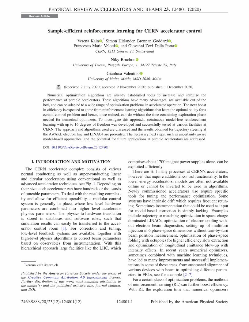
The AWAKE electron source and line are particularlyinteresting for proof-of-concept tests for various algorithmsdue to the high repetition rate, various types of beaminstrumentation and insignificant damage potential in caseof losing the beam at accelerator components. The first RLagents were trained for trajectory correction on theAWAKE electron line with the goal that the trained agentscorrect the line with a similar efficiency as the responsematrix based SVD algorithm that is usually used in thecontrol room, i.e., correction to a similar RMS as SVDwithin ideally 1 iteration. Figure 4 shows an example of acorrection using the SVD implementation as available inthe control room.The AWAKE electrons are generated in a 5 MV RF gun,

accelerated to 18 MeVand then transported through a beamline of 12 m to the AWAKE plasma cell. A vertical step of1 m and a 60° bend bring the electron beam parallel to theproton beam shortly before the plasma cell. The trajectory

VERENA KAIN et al. PHYS. REV. ACCEL. BEAMS 23, 124801 (2020)

124801-4

is controlled with 11 horizontal and 11 vertical steeringdipoles according to the measurements of 11 beam positionmonitors (BPMs). The BPM electronic read out is at 10 Hzand acquisition through the CERN middleware at 1 Hz.For reference, numerical optimizers had been tested as

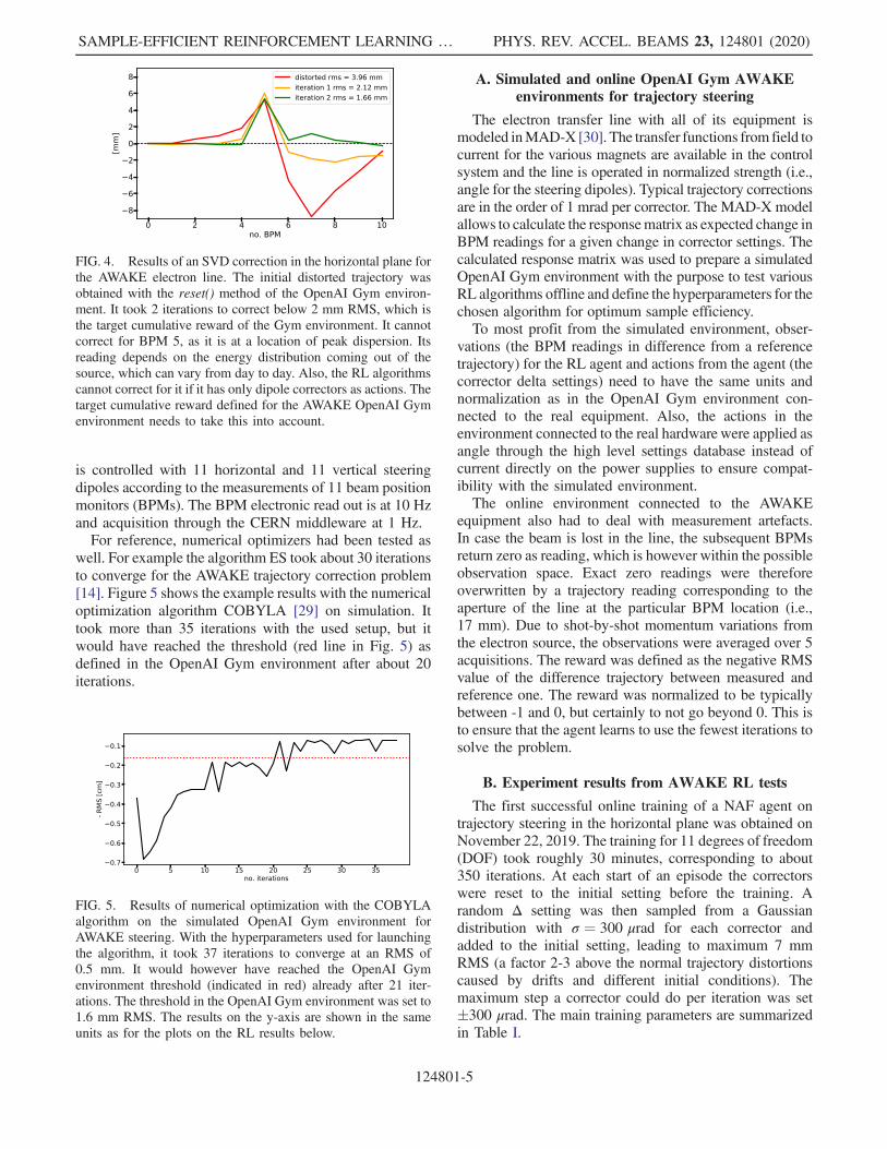
well. For example the algorithm ES took about 30 iterationsto converge for the AWAKE trajectory correction problem[14]. Figure 5 shows the example results with the numericaloptimization algorithm COBYLA [29] on simulation. Ittook more than 35 iterations with the used setup, but itwould have reached the threshold (red line in Fig. 5) asdefined in the OpenAI Gym environment after about 20iterations.

A. Simulated and online OpenAI Gym AWAKEenvironments for trajectory steering

The electron transfer line with all of its equipment ismodeled inMAD-X [30]. The transfer functions from field tocurrent for the various magnets are available in the controlsystem and the line is operated in normalized strength (i.e.,angle for the steering dipoles). Typical trajectory correctionsare in the order of 1 mrad per corrector. The MAD-X modelallows to calculate the responsematrix as expected change inBPM readings for a given change in corrector settings. Thecalculated response matrix was used to prepare a simulatedOpenAI Gym environment with the purpose to test variousRL algorithms offline and define the hyperparameters for thechosen algorithm for optimum sample efficiency.To most profit from the simulated environment, obser-

vations (the BPM readings in difference from a referencetrajectory) for the RL agent and actions from the agent (thecorrector delta settings) need to have the same units andnormalization as in the OpenAI Gym environment con-nected to the real equipment. Also, the actions in theenvironment connected to the real hardware were applied asangle through the high level settings database instead ofcurrent directly on the power supplies to ensure compat-ibility with the simulated environment.The online environment connected to the AWAKE

equipment also had to deal with measurement artefacts.In case the beam is lost in the line, the subsequent BPMsreturn zero as reading, which is however within the possibleobservation space. Exact zero readings were thereforeoverwritten by a trajectory reading corresponding to theaperture of the line at the particular BPM location (i.e.,17 mm). Due to shot-by-shot momentum variations fromthe electron source, the observations were averaged over 5acquisitions. The reward was defined as the negative RMSvalue of the difference trajectory between measured andreference one. The reward was normalized to be typicallybetween -1 and 0, but certainly to not go beyond 0. This isto ensure that the agent learns to use the fewest iterations tosolve the problem.

B. Experiment results from AWAKE RL tests

The first successful online training of a NAF agent ontrajectory steering in the horizontal plane was obtained onNovember 22, 2019. The training for 11 degrees of freedom(DOF) took roughly 30 minutes, corresponding to about350 iterations. At each start of an episode the correctorswere reset to the initial setting before the training. Arandom Δ setting was then sampled from a Gaussiandistribution with σ ¼ 300 μrad for each corrector andadded to the initial setting, leading to maximum 7 mmRMS (a factor 2-3 above the normal trajectory distortionscaused by drifts and different initial conditions). Themaximum step a corrector could do per iteration was set�300 μrad. The main training parameters are summarizedin Table I.

FIG. 4. Results of an SVD correction in the horizontal plane forthe AWAKE electron line. The initial distorted trajectory wasobtained with the reset() method of the OpenAI Gym environ-ment. It took 2 iterations to correct below 2 mm RMS, which isthe target cumulative reward of the Gym environment. It cannotcorrect for BPM 5, as it is at a location of peak dispersion. Itsreading depends on the energy distribution coming out of thesource, which can vary from day to day. Also, the RL algorithmscannot correct for it if it has only dipole correctors as actions. Thetarget cumulative reward defined for the AWAKE OpenAI Gymenvironment needs to take this into account.

FIG. 5. Results of numerical optimization with the COBYLAalgorithm on the simulated OpenAI Gym environment forAWAKE steering. With the hyperparameters used for launchingthe algorithm, it took 37 iterations to converge at an RMS of0.5 mm. It would however have reached the OpenAI Gymenvironment threshold (indicated in red) already after 21 iter-ations. The threshold in the OpenAI Gym environment was set to1.6 mm RMS. The results on the y-axis are shown in the sameunits as for the plots on the RL results below.

SAMPLE-EFFICIENT REINFORCEMENT LEARNING … PHYS. REV. ACCEL. BEAMS 23, 124801 (2020)

124801-5

The objective of the training was twofold: to maximizethe reward from each initial condition, and to maximize thereward in the shortest possible time. Figure 6 shows theevolution of the 200 episode online training. The upper plotgives the length of the episodes in number of iterations astraining evolves, while the lower plot shows the initialreward (i.e., negative RMS) at the beginning of the episode(green line) as well as the final reward achieved (blue line)at the end of each episode. For a successful termination ofthe episode, the final reward had to be above the target(dashed red line).At the beginning of the training, the agent could not

correct the line to an RMS below 2 mm, despite manyiterations. It even further deteriorated the trajectory. Afterabout 15 episodes it had learned to successfully correct thetrajectory within 1-2 iterations to mostly even below 1 mmRMS starting from any initial condition. Figure 7 shows theevolution of the value function VðsÞ and the loss functionfor the network training as a function of iterations. Thevalue function started to stabilize after about 90 iterations(equivalent to the 15 episodes when successful correctionwas observed), continued to improve for another 100iterations and finally converged to −0.05 correspondingto 0.5 mm RMS after correction in case of only oneiteration required. After the online training where explora-tion noise is still present (albeit decaying very rapidly withincreasing episode number), the agent was tested in anoperational configuration. No noise is added to the actions

predicted by the trained agent in this case. The agent waspresented with randomly sampled observations (by invok-ing the reset() method of the environment) and it had tocorrect the line accordingly. Figure 8 shows the validationrun with 24 episodes. The plot is arranged as for thetraining results above, with the upper plot showing thenumber of iterations per episodes and the lower one,the initial and final negative RMS per episode. The trainedagent required 1 or 2 iterations to correct the trajectory tobetter than the target (it requires more than 1 iteration fromtime to time as its maximum step per iteration is limited to300 μrad). A longer validation run was carried out begin-ning of June 2020 with an agent that had only been trainedfor 35 episodes. The results of this validation can be foundin Fig. 9.

TABLE I. AWAKE horizontal steering NAF agent trainingparameters.

DOF 11Reward target [cm] −0.2Max episode length 50Max Δcorr [μrad] 300Min allowed reward [cm] −1.2

FIG. 6. Online training of NAF agent of AWAKE electron linetrajectory steering in the horizontal plane. In the upper plot thenumber of iterations per episode is given. The lower plot showsthe initial and final negative RMS value for each episode. Thetarget negative RMS value is indicated in red.

FIG. 7. Evolution of loss and value function during training onNovember 22, 2019.

FIG. 8. Short validation run after training with 200 episodes onNovember 22, 2019. The agent corrects the trajectory to betterthan 2 mm RMS target within 1-2 iterations. (The initialtrajectories were established by randomly applying correctorsettings, which can lead to initial trajectories already above thetarget. In the test setup no check on initial RMS was used beforecalling the agent and it would therefore correct trajectoriesalready above target generalizing from the training earlier, withfew trajectories in this region as episodes would be finalized atthat stage. All results are above target, but trajectories withinitially very good RMS were sometimes slightly deterioratedbecause of this test setup artefact. The test setup was improved forthe next validations.)

VERENA KAIN et al. PHYS. REV. ACCEL. BEAMS 23, 124801 (2020)

124801-6

An important question is also how long a trainingremains valid and how often an RL agent would have tobe re-trained. Obviously this depends on the specificproblem and how much state information is hidden. Inour case the expectation was that if the agent is trainedonce, it will not need any re-training unless the lattice of theline is changed. To verify this expectation, a NAF agenttrained on June 10, 2020, was successfully re-validatedon September 22, 2020, without any additional training.The validation results are shown in Fig. 10.Another important application of RL will result from

training RL agents on simulation and then exploit the agentwith or without additional short training on the accelerator.The obvious advantage of this approach, if possible, is thatin this case the algorithm does not have to be restrictedto be a very sample-efficient one, as accelerator time fortraining is either zero or limited. To test this principleof offline training, another NAF agent was trained—this time on the simulated AWAKE trajectory correctionenvironment. This agent was then used on the accelerator inoperational configuration as trajectory correction algorithm.

As expected, the results—maximum 2 iterations for correc-tion to well below 2 mm RMS for each episode—were asgood as with the online trained agent. Figure 11 shows theresults.

IV. RL AGENT FOR LINAC4 TRAJECTORYCORRECTION

Training the AWAKE RL agent for trajectory correctionwas a test case for algorithm development, since classicaloptics model-based steering algorithms are available for theAWAKE 18 MeV beamline. The CERN LINACs, on theother hand, do not have online models, since the approachfor defining models in the control system developed fortransfer lines and the synchrotrons does not fit LINACSswithout adaptation. Beam parameters are usually tunedmanually, guided by offline calculations and experience.RL and numerical optimization could be obvious andinexpensive solutions to many typical LINAC tuningproblems. The CERN accelerator complex comprisestwo LINACs. LINAC3 is used for a variety of ions andthe 160 MeV LINAC4 will provide H− to the upgradedCERN proton chain through charge exchange injection intothe PS Booster [31]. LINAC4 had its final commissioningrun at the end of 2019, where some time was also allocatedto test various advanced algorithms for different controlproblems. Figure 12 shows an example of numericalopimization with the algorithm COBYLA for trajectorycorrection in LINAC4. Also, an RL agent using the NAFalgorithm was trained for trajectory steering in the LINACexploiting the experience with AWAKE.LINAC4 accelerates H− from 3 MeV after source and

RFQ to 160 MeV. The medium energy beam transport(MEBT) after the RFQ is followed by a conventional drifttube linac (DTL) of about 20 m that accelerates the ions to50 MeV, then to 100 MeV in 23 m by a cell-coupled drifttube LINAC (CCDTL) and finally to 160 MeV by aπ-mode structure (PIMS). The total length of the LINACup to the start of the transfer line to the PSB is roughly75 m. The pulse repetition rate is 0.83 Hz. The trajectory in

FIG. 9. Validation right after short training of 35 episodes onJune 8, 2020. Despite the short training, the agent corrects thetrajectory to better than the 2 mm RMS target within 1-3iterations.

FIG. 10. Validation on accelerator on September 22, 2020, ofagent that was trained more than three months earlier (June 10,2020). The agent corrects the trajectory to better than 2 mm RMSwithin 1-2 iterations. No retraining was required.

FIG. 11. Validation on accelerator of agent that was trained onsimulation. The agent corrects the trajectory to better than 2 mmRMS within 1-2 iterations.

SAMPLE-EFFICIENT REINFORCEMENT LEARNING … PHYS. REV. ACCEL. BEAMS 23, 124801 (2020)

124801-7

the MEBT is fine tuned for optimizing chopping efficiencyand should not be modified during general trajectoryoptimization. In addition there are no BPMs available inthe MEBT as observable for an RL agent.

A. Online OpenAI Gym LINAC4 environment

The LINAC4 Gym environment comprised state infor-mation from 17 BPMs and actions possible on 16 correc-tors, through DTL, CCDTL, PIMS and start of the transferline in the horizontal plane (the allocated acceleratordevelopment time was not sufficient to also train for thevertical plane). No simulated environment was available forthis case and the tuning of the hyperparameters had to becarried out online. The hyperparameters obtained earlierwith AWAKE were not directly re-usable as the allowedtrajectory excursion range was much reduced due tomachine protection reasons (e.g., the maximum allowedRMS had to be set to 3 mm, which affected the normali-zation of the returned reward). The LINAC4 trajectorysteering OpenAI Gym environment had to respect themachine protection constraints and finalize episodes incase of violation, reset to safe settings as well as to dealwith various hardware limitations (e.g., the power suppliesthe steering dipoles cannot regulate for jIj < 0.1 A).

B. Experimental results from LINAC4 RL tests

LINAC4 had 8 weeks of final commissioning run in2019. On November 27, half a day was allocated to trainingand testing the NAF agent. A big fraction of this timewas used in fine tuning hyperparameters such that theagent would not immediately run into rather tight machineprotection limits during the exploration phase. A successfultraining could be achieved, with the agent training param-eters given in Table II. The training is shown in Fig. 13

and the convergence of the value function VðsÞ and lossfunction in Fig. 14. The total number of episodes was set to90 (taking in total about 300 iterations).After about 25 episodes (or the equivalent of about 125

iterations), the agent had learned to correct the trajectory tobelow 1 mm RMS within a maximum of 3 iterations eachtime. The value function converged to -0.85 correspondingto 0.85 mm RMS in case of correction in one iteration.No other tests could be performed at that stage due to lackof time. It would obviously be of interest to deploy the

FIG. 12. Optimization with COBYLA of the LINAC4 trajec-tory correction problem in the horizontal plane. The algorithmconverged after around 70 iterations.

FIG. 14. Online training of NAF agent on LINAC4 trajectorysteering in horizontal plane: convergence of loss function andvalue function V. The latter converges to −0.85 corresponding toan RMS better than 1 mm in case of correction in one iteration.

TABLE II. LINAC4 horizontal steering NAF agent trainingparameters.

DOF 16Reward target [mm] −1Max episode length 15Max Δcorr [A] 0.5Min allowed reward [mm] −3

FIG. 13. Online training of NAF agent on LINAC4 trajectorysteering in horizontal plane. The maximum allowable RMS waslimited to 3 mm due to machine protection reasons. The target forthe training was set to reach 1 mm RMS.

VERENA KAIN et al. PHYS. REV. ACCEL. BEAMS 23, 124801 (2020)

124801-8

trained agent as part of the standard LINAC4 control roomtools for the 2020 run and to test long term stability.

V. DISCUSSION AND OUTLOOK

The experience with the AWAKE and LINAC4 RL agentdeployment has proved that the question of sample effi-ciency for the model-free RL approach can be addressed forreal accelerator control problems. The training with algo-rithms such as NAF (and TD3) is sample-efficient enoughto allow for deployment in the control room. It requiresmore iterations than a numerical optimization algorithm,but after training it outperforms numerical optimizers. Theresulting product is a control algorithm like SVD. Whereasthe linear control problem of trajectory correction can besolved with SVD or other standard methods, single-stepcorrection for nonlinear problems are not availablewith thesestandard algorithms. RL does not require a linear responseand can thus provide controllers for also these cases.The standardization of the environment description using

OpenAI Gym proved a big advantage, allowing rapidswitching between simulated and online training, andbetween agents. Correct normalization and un-normaliza-tion of all actions, state observations and rewards was ofcourse crucial. For the training, care needed to be taken inconstructing the reward function and episode terminationcriteria. The key hyperparameters were found to be themaximum number of iterations per episode, and the rewardtarget for early episode termination. Note that these hyper-parameters belong to the environment description and notto algorithms themselves. The same environment hyper-parameters can be used with different RL algorithms e.g.,NAF and TD3. Tuning of these hyperparameters took sometime, and valuable experience was gained from having asimulated AWAKE environment, although such a simulatedenvironment cannot be counted on for many applicationdomains and indeed was not available for the LINAC4tests. Also, the algorithms come with hyperparameters, butthe default parameters gave mostly already very goodresults.Model-free RL algorithms have the advantage of limited

complexity and insignificant computer power require-ments. The most sample-efficient algorithms (i.e., NAF,TD3) are straightforward to tune and can solve acceleratorcontrol problems, as shown in this paper. For acceleratorswith a lower repetition rate (e.g., repetition period of>1 minute), the number of iterations needs to be evenfurther reduced to allow for stable training conditions oreven allow for the training at all, given that accelerator timeis expensive and normally overbooked. Model-based RL isa promising alternative to overcome the sample efficiencylimitation, depending on the algorithm, however, at theexpense of requiring significant computing resources.Another advantage of these algorithms is that an explicitmodel of the control problem response is a byproduct of thetraining of the agent.

The beam time reserved for advanced algorithms in 2020at AWAKE will be used to deploy various model-based RLalgorithms as well as model predictive control such as theiLQR [16] algorithm on a model obtained through super-vised learning.Another general challenge for RL agents next to the

question of sample efficiency, addressed in this paper, is theavailability of meaningful state observation. The RL agentfor the automatching [32] of AWAKE source initial con-ditions to the transfer line lattice uses computer visionmachine learning algorithms for the interpretation of OTRscreen measurements, to implicitly encode the state.In addition to studying new algorithms, infrastructure

and frameworks will have to be deployed in the controlsystem to easily make use of advanced algorithms andmachine learning. This is also part of the goal for the 2020AWAKE tests, where we aim to provide a generic opti-mization framework for the control room, includingcentrally stored neural networks as well as registeringenvironments and algorithms for common use.

VI. CONCLUSIONS

Modern particle accelerators are complex, with often verydense user schedules, and need to be exploited efficiently.Deterministic operation and automation are the cornerstonesfor a new operations paradigm. Numerical optimizers arealready used on a regular basis in the control room, forapplications inaccessible to classical correction algorithms.With the recent progress in the field of deep reinforcementlearning, parameter tuning in the control room can be learnedby algorithms to further boost efficiency and extend theapplication domain. Not only are these algorithms readilyavailable, but they are also straightforward to tune.In this paper the sample-efficient RL algorithm NAF was

successfully trained on real-world accelerator tuning prob-lems with the trajectory steering agents at the CERNAWAKE electron line and the H− accelerator LINAC4.We have also shown the potential of transfer learning for anRL agent, by training it on simulation and applying it on thereal accelerator successfully with no retraining needed.The main challenge is the implementation of the domain

specific optimization problem with the adequate definitionof reward in the chosen OpenAI Gym environments.Several guidelines are compiled in this paper to help withthat task.Only model-free RL algorithms were tested as part of

this initial study. Model-free algorithms have insignificantrequirements on computing infrastructure, but model-basedones have additional interesting advantages, particularlyfurther increased sample efficiency. They will be part of thenext test series.Last but not least, as machine learning in all its forms

will inevitably be part of operating particle accelerators,this work has shown that controls infrastructure will have toprovide for storing and retrieving neural networks centrally

SAMPLE-EFFICIENT REINFORCEMENT LEARNING … PHYS. REV. ACCEL. BEAMS 23, 124801 (2020)

124801-9

along with algorithms and the equivalent to OpenAI Gymenvironments.

APPENDIX A: COMPARISON: Q LEARNINGVERSUS ON-POLICY REINFORCEMENT

LEARNING

The NAF algorithm was compared with the state-of-the-art on policy algorithm PPO [33], see Fig. 15. As expectedfrom literature, Q learning is more sample-efficient than on-policy learning—by at least one order of magnitude for thisspecific problem. A comparison between the TD3 algo-rithm and the implementation of NAF with prioritizedexperience replay is given in Fig. 16.

APPENDIX B: PER-NAF DETAILS

1. Network and training parameter details

The NAF network architecture as described in this paperwas used with activation function tanh(). The weights wereinitialized to be within ð−0.05; 0.05Þ at the beginning of thetraining and the learning rate α was set to 1 × 10−3 with abatch size of 50. For the Q-learning, a discount factor ofγ ¼ 0.999 was applied and τ for the soft target update wasset to τ ¼ 0.001.

2. The prioritization of the samples

The data distribution for off-policy algorithms likeQ-learning is crucial and current research proposes severalstrategies [34,35]. New data is gathered online followingthe current policy, while off-line data from the replay bufferis used to improve the policy. In our implementation, thedata selected to minimize the loss function, or temporaldifference error, during the training is weighted accordingto their previous temporal difference error. Data with alarger error is used more often for the weight update thanother data [25]. Two parameters, α and β are important tocontrol the priority and the weighting of the samples. Theprobability Pi to select a sample i from the replay buffer is

Pi ¼lαiPkl

αi; ðB1Þ

where li is the temporal difference error of sample i. Thesample is used with the weight wi

wi ¼�1

N1

Pi

�β

ðB2Þ

For the NAF agents in this paper α and β were chosen tobe 0.5.Figure 17 shows a comparison of the obtained cumu-

lative reward for different seeds during a training with thesimulated Gym environment of AWAKE. The blue and redcurves were obtained with prioritization (blue β ¼ 0.5 andred β ¼ 0.9), the green curve without. The variance of theresults is smaller in case of using prioritization and thetraining faster such that higher cumulative rewards arereached earlier.

3. The exploration policy

For exploration during the training in the experimentsdiscussed in this paper, Gaussian random noise was addedto the proposed actions with a standard deviation σ ¼ 1decaying with 1=ð0.1 × nþ 1Þ, where n is the episodenumber. In Fig. 18 this exploration strategy, which islabeled as inverse strategy in the plot, is compared to astrategy with a standard deviation reduced linearly over 100episodes, labeled as linear strategy. The upper plot showsthe reduction of the standard deviation for the Gaussian

FIG. 15. A comparison between the on-policy state-of-the-artalgorithm PPO and the NAF algorithm for the AWAKE trajectorycorrection problem. The cumulative reward was averaged overfive different random seeds.

FIG. 16. A comparison between the state-of-the-art TD3algorithm and PER-NAF on the AWAKE simulated environment.The overall performance is comparable.

VERENA KAIN et al. PHYS. REV. ACCEL. BEAMS 23, 124801 (2020)

124801-10

random noise as function of episode and the lower plot thecumulative reward per episode obtained for training withfive different seeds. The inverse strategy results in a morestable training.

[1] D. Jacquet, R. Gorbonosov, and G. Kruk, LSA—The HighLevel Application Software of the LHC and its Perfor-mance during the first 3 years of Operation, 14thInternational Conference on Accelerator & Large Exper-imental Physics Control Systems,San Francisco, CA, USA, 6–11 Oct 2013, pp. thppc058,https://cds.cern.ch/record/1608599.

[2] A. Edelen, N. Neveu, M. Frey, Y. Huber, C. Mayes, and A.Adelmann, Machine learning for orders of magnitudespeedup in multiobjective optimization of particle accel-erator systems, Phys. Rev. Accel. Beams 23, 044601(2020).

[3] G. Azzopardi, A. Muscat, G. Valentino, S. Redaelli, and B.Salvachua, Operational results of LHC collimator alignmentusing machine learning, in Proc. IPAC’19, Melbourne,Australia (JACoW, Geneva, 2019), pp. 1208–1211.

[4] S. Hirlaender, M. Fraser, B. Goddard, V. Kain, J. Prieto, L.Stoel, M. Szakaly, and F. Velotti, Automatisation of theSPS ElectroStatic Septa Alignment, in 10th Int. ParticleAccelerator Conf.(IPAC’19) (JACoW, Geneva, 2019),p. 4001–4004.

[5] J. Duris et al., Bayesian Optimization of a Free-ElectronLaser, Phys. Rev. Lett. 124, 124801 (2020).

[6] A. Hanuka et al., Online tuning and light source controlusing a physics-informed Gaussian process Adi, https://arxiv.org/abs/1911.01538.

[7] M. McIntire et al., Sparse Gaussian processes for Bayesianoptimization, https://www-cs.stanford.edu/~ermon/papers/sparse-gp-uai.pdf.

[8] N. Bruchon, G. Fenu, G. Gaio, M. Lonza, F. A. Pellegrino,and E. Salvato, Toward the Application of ReinforcementLearning to the Intensity Control of a Seeded Free-ElectronLaser, 2019 23rd International Conference on Mecha-tronics Technology (ICMT), SALERNO, Italy, 2019,pp. 1–6, https://doi.org/10.1109/ICMECT.2019.8932150.

[9] N. Bruchon, G. Fenu, G. Gaio, M. Lonza, F. H. O’Shea,F. A. Pellegrino, and E. Salvato, Basic reinforcementlearning techniques to control the intensity of a seededfree-electron laser, Electronics 9, 781 (2020).

[10] T. Boltz et al., Feedback design for control of the micro-bunching instability based on reinforcement learning, in10th Int. Particle Accelerator Conf.(IPAC’19), https://doi.org/10.18429/JACoW-IPAC2019-MOPGW017.

[11] A. Edelen et al., Using a neural network control policy forrapid switching between beam parameters in an FEL, in38th International Free Electron Laser Conference,https://doi.org/10.18429/JACoW-FEL2017-WEP031.

[12] E. Shaposhnikova et al., LHC injectors upgrade (LIU)project at CERN, in 7th International Particle AcceleratorConference, Busan, Korea, 8–13 May 2016, pp. MO-POY059, https://doi.org/10.18429/JACoW-IPAC2016-MO-POY059.

[13] E. Adli, A. Ahuja, O. Apsimon, R. Apsimon, A.-M.Bachmann, D. Barrientos, F. Batsch, J. Bauche, V. B.Olsen, M. Bernardini et al., Acceleration of electrons inthe plasma wakefield of a proton bunch, Nature (London)561, 363 (2018).

[14] A. Scheinker, S. Hirlaender, F. M. Velotti, S. Gessner, G. Z.Della Porta, V. Kain, B. Goddard, and R. Ramjiawan,Online multi-objective particle accelerator optimization ofthe AWAKE electron beam line for simultaneous emittanceand orbit control, AIP Adv. 10, 055320 (2020).

[15] R. Sutton and A. Barto, Introduction to ReinforcementLearning (MIT Press, Cambridge, MA, USA, 2018).

[16] H. Kwakernaak and R. Sivan, Linear Optimal ControlSystems (Wiley-Interscience, New York, 1972).

[17] A.Nagabandi, G.Kahn, R. S. Fearing, and S. Levine,Neuralnetwork dynamics for model-based deep reinforcementlearning with model-free fine-tuning, arXiv:1708.02596.

[18] R. Sutton, Dyna, an integrated architecture for learning,planning, and reacting, AAAI Spring Symposium 2, 151(1991).

FIG. 18. Two exploration strategies: the inverse strategy resultsin a more stable training.

FIG. 17. The training with prioritization of the samples fortwo different values of β compared to the baseline withoutprioritization.

SAMPLE-EFFICIENT REINFORCEMENT LEARNING … PHYS. REV. ACCEL. BEAMS 23, 124801 (2020)

124801-11

[19] T. Wang et al., Benchmarking model-based reinforcementlearning, https://arxiv.org/abs/1907.02057v1.

[20] V. Mnih et al., Human-level control through deepreinforcement learning, Nature (London) 518, 529 (2015).

[21] T. Lillicrap et al., Continuous control with deep reinforce-ment learning, in Proc. ICLR 2016, https://arxiv.org/abs/1509.02971.

[22] S. Gu, T. Lillicrap, I. Sutskever, and S. Levine, Continuousdeep Q-learning with model-based acceleration, in Proc.33rd International Conference on Machine Learning,New York, NY, USA, 2016 [arXiv:1603.00748].

[23] S. Fujimoto, H. van Hoof, and D. Meger, Addressingfunction approximation error in actor-critic methods,arXiv:1802.09477.

[24] Y. Gal, R. McAllister, and C. E. Rasmussen, ImprovingPILCO with Bayesian neural network dynamics models,in Data-Efficient Machine Learning workshop, ICML 4, 34(2016).

[25] T. Schaul, J. Quan, I. Antonoglou, and D. Silver, Priori-tized experience replay, arXiv:1511.05952.

[26] S. Hirlaender, PER-NAF available at https://github.com/MathPhysSim/PER-NAF/ and https://pypi.org/project/pernaf/.

[27] PYJAPC available at https://pypi.org/project/pyjapc/.

[28] http://gym.openai.com.[29] M. J. D. Powell, A direct search optimization method that

models the objective and constraint functions by linearinterpolation, in Advances in Optimization and NumericalAnalysis, edited by S. Gomez and J.-P. Hennart (KluwerAcademic, Dordrecht, 1994), pp. 51–67.

[30] MAD-X documentation and source code available athttps://mad.web.cern.ch/mad/.

[31] G. Bellodi, Linac4 commissioning status and challenges tonominal operation, 61st ICFA Advanced Beam DynamicsWorkshop on High-Intensity and High-Brightness HadronBeams, Daejeon, Korea, 17–22 Jun 2018, pp. MOA1PL03,https://doi.org/10.18429/JACoW-HB2018-MOA1PL03.

[32] F. Velotti, B. Goddard et al., Automatic AWAKE electronbeamline setup using unsupervised machine learning (to bepublished).

[33] J. Schulmann et al., Proximal policy optimization algo-rithms, https://arxiv.org/pdf/1707.06347.pdf.

[34] A. Kumar, A. Gupta, and S. Levine, DisCor: Correctivefeedback in reinforcement learning via distribution cor-rection, arXiv:2003.07305.

[35] A. Kumar, J. Fu, G. Tucker, and S. Levine, Stabilizing off-policy Q-learning via bootstrapping error reduction, arXiv:1906.00949.

VERENA KAIN et al. PHYS. REV. ACCEL. BEAMS 23, 124801 (2020)

124801-12