physical-chemistry ii chapter-2-the rates of chemical ... · physical-chemistry ii chapter-2-the...
TRANSCRIPT

Physical-Chemistry II
Chapter-2-The rates of chemical reactions
الكيميائيةسرعات التفاعالت
Dr. El Hassane ANOUAR
Chemistry Department, College of Sciences and Humanities, Prince Sattam bin
Abdulaziz University, P.O. Box 83, Al-Kharij 11942, Saudi Arabia.
4/28/2017 College of Science and humanities, Al-kharj 1
Physical
Chemistry II
(Chem 3320)
Important :
These slides are prepared in reference to chapter 21 in Physical Chemistry, Ninth
Edition, Peter Atkins, and Julio De Paula

4/28/2017 College of Science and humanities, Al-kharj 2
3. Examples of reaction mechanisms
3.1 Unimolecular reactions
First-order gas-phase reactions are widely called ‘unimolecular reactions’
because they also involve an elementary unimolecular step in which the reactant
molecule changes into the product.
Example: The isomerization of cyclopropane:
𝐜𝐲𝐜𝐥𝐨 − 𝐂𝟑𝐇𝟔 → 𝐂𝐇𝟑𝐂𝐇 = 𝐂𝐇𝟐 𝒗 = 𝐤𝐫 [𝐜𝐲𝐜𝐥𝐨 − 𝐂𝟑𝐇𝟔]
In a first-order rate laws, presumably a molecule acquires enough energy to react
as a result of its collisions with other molecules.
However, collisions are simple bimolecular events, so how can they result in a
first-order rate law?
The overall mechanism has bimolecular as well as unimolecular steps.

4/28/2017 College of Science and humanities, Al-kharj 3
3.1.2 The Lindemann–Hinshelwood mechanism
3. Examples of reaction mechanisms
3.1 Unimolecular reactions
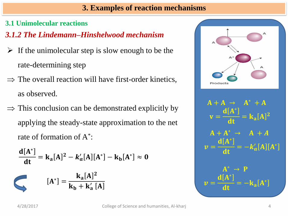
In Lindemann–Hinshelwood mechanism, it is supposed
that a reactant molecule A becomes energetically excited
by collision with another A molecule in a bimolecular
step. 𝐀 + 𝐀 → 𝐀∗ + 𝐀 𝐯 =
𝐝 𝐀∗
𝐝𝐭= 𝐤𝐚 𝐀
𝟐
A* might lose its excess energy by collision
with another molecule
𝐀 + 𝐀∗ → 𝐀 + 𝑨
𝒗 =𝐝 𝐀∗
𝐝𝐭= −𝒌𝒂
′ 𝐀 𝐀∗
Alternatively, A* might shake itself apart and form
products P (i.e., it might undergo the unimolecular
decay
𝐀∗ → 𝐏
𝒗 =𝐝 𝐀∗
𝐝𝐭= −𝐤𝒃 𝐀
∗
4/28/2017 College of Science and humanities, Al-kharj 4
3.1.2 The Lindemann–Hinshelwood mechanism
3. Examples of reaction mechanisms
3.1 Unimolecular reactions
𝐀 + 𝐀 → 𝐀∗ + 𝐀
𝐯 =𝐝 𝐀∗
𝐝𝐭= 𝐤𝐚 𝐀
𝟐
𝐀 + 𝐀∗ → 𝐀 + 𝑨
𝒗 =𝐝 𝐀∗
𝐝𝐭= −𝒌𝒂
′ 𝐀 𝐀∗
𝐀∗ → 𝐏
𝒗 =𝐝 𝐀∗
𝐝𝐭= −𝐤𝐚 𝐀
∗
If the unimolecular step is slow enough to be the
rate-determining step
The overall reaction will have first-order kinetics,
as observed.
This conclusion can be demonstrated explicitly by
applying the steady-state approximation to the net
rate of formation of A*:
𝐝 𝐀∗
𝐝𝐭= 𝐤𝐚 𝐀
𝟐 − 𝒌𝒂′ 𝐀 𝐀∗ − 𝐤𝐛 𝐀
∗ ≈ 𝟎
𝐀∗ =𝐤𝐚 𝐀
𝟐
𝐤𝐛 + 𝐤𝐚′ 𝐀

4/28/2017 College of Science and humanities, Al-kharj 5
3.1.2 The Lindemann–Hinshelwood mechanism
3. Examples of reaction mechanisms
3.1 Unimolecular reactions
𝐀 + 𝐀 → 𝐀∗ + 𝐀
𝐯 =𝐝 𝐀∗
𝐝𝐭= 𝐤𝐚 𝐀
𝟐
𝐀 + 𝐀∗ → 𝐀 + 𝑨
𝒗 =𝐝 𝐀∗
𝐝𝐭= −𝒌𝒂
′ 𝐀 𝐀∗
𝐀∗ → 𝐏
𝒗 =𝐝 𝐀∗
𝐝𝐭= −𝐤𝐚 𝐀
∗
𝐝 𝐏
𝐝𝐭= 𝐤𝐛 𝐀
∗ =𝐤𝐚𝐤𝐛 𝐀
𝟐
𝐤𝐛 + 𝐤𝐚′ 𝐀
So, the rate law for the formation of P is
At this stage the rate law is not first-order.
However, if the rate of deactivation by (A*,A) collisions
is much greater than the rate of unimolecular decay:
ka′ A A∗ ≫ kb A
∗ or ka′ A ≫ kb
Thus 𝐝 𝐏
𝐝𝐭= 𝐤𝐫 𝐀 ; 𝐤𝐫 =
𝐤𝐚𝐤𝐛𝐤𝐚′
Is a first-order rate law
4/28/2017 College of Science and humanities, Al-kharj 6
3.1.2 The Lindemann–Hinshelwood mechanism
3. Examples of reaction mechanisms
3.1 Unimolecular reactions
𝐀 + 𝐀 → 𝐀∗ + 𝐀
𝐯 =𝐝 𝐀∗
𝐝𝐭= 𝐤𝐚 𝐀
𝟐
𝐀 + 𝐀∗ → 𝐀 + 𝑨
𝒗 =𝐝 𝐀∗
𝐝𝐭= −𝒌𝒂
′ 𝐀 𝐀∗
𝐀∗ → 𝐏
𝒗 =𝐝 𝐀∗
𝐝𝐭= −𝐤𝐚 𝐀
∗
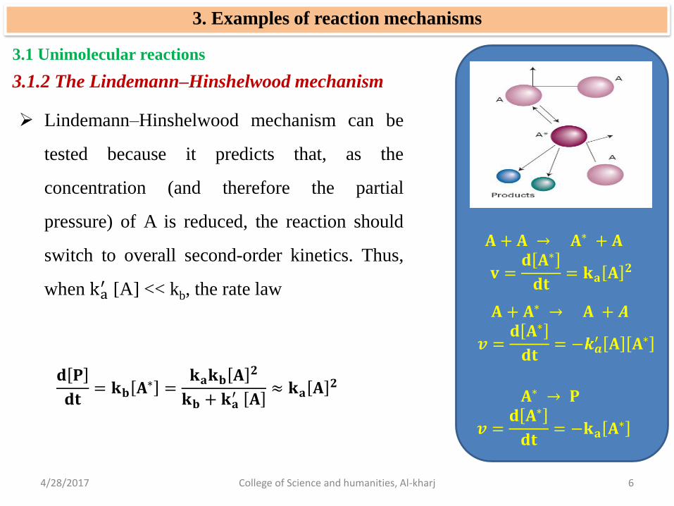
Lindemann–Hinshelwood mechanism can be
tested because it predicts that, as the
concentration (and therefore the partial
pressure) of A is reduced, the reaction should
switch to overall second-order kinetics. Thus,
when ka′ [A] << kb, the rate law
𝐝 𝐏
𝐝𝐭= 𝐤𝐛 𝐀
∗ =𝐤𝐚𝐤𝐛 𝐀
𝟐
𝐤𝐛 + 𝐤𝐚′ 𝐀≈ 𝐤𝐚 𝐀
𝟐
4/28/2017 College of Science and humanities, Al-kharj 7
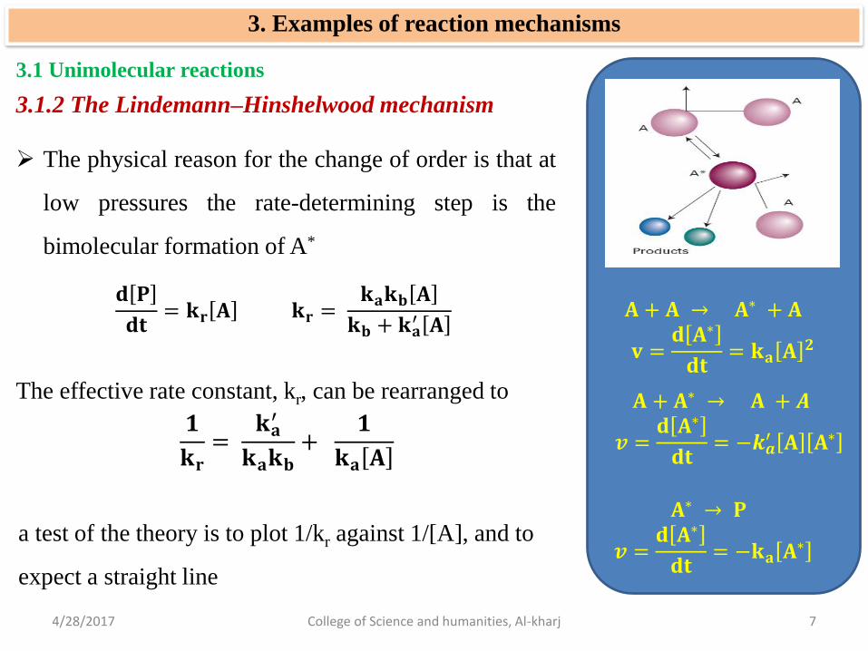
The physical reason for the change of order is that at
low pressures the rate-determining step is the
bimolecular formation of A*
3.1.2 The Lindemann–Hinshelwood mechanism
3. Examples of reaction mechanisms
3.1 Unimolecular reactions
𝐀 + 𝐀 → 𝐀∗ + 𝐀
𝐯 =𝐝 𝐀∗
𝐝𝐭= 𝐤𝐚 𝐀
𝟐
𝐀 + 𝐀∗ → 𝐀 + 𝑨
𝒗 =𝐝 𝐀∗
𝐝𝐭= −𝒌𝒂
′ 𝐀 𝐀∗
𝐀∗ → 𝐏
𝒗 =𝐝 𝐀∗
𝐝𝐭= −𝐤𝐚 𝐀
∗
𝐝 𝐏
𝐝𝐭= 𝐤𝐫 𝐀 𝐤𝐫 =
𝐤𝐚𝐤𝐛 𝐀
𝐤𝐛 + 𝐤𝐚′ 𝐀
The effective rate constant, kr, can be rearranged to
𝟏
𝐤𝐫= 𝐤𝐚′
𝐤𝐚𝐤𝐛+ 𝟏
𝐤𝐚 𝐀
a test of the theory is to plot 1/kr against 1/[A], and to
expect a straight line

4/28/2017 College of Science and humanities, Al-kharj 8
3.1.2 The activation energy of a composite reaction
3. Examples of reaction mechanisms
3.1 Unimolecular reactions
Although the rate of each step of a complex
mechanism might increase with temperature and
show Arrhenius behaviour. Is that true of a
composite reaction? 𝐀 + 𝐀 → 𝐀∗ + 𝐀
𝐯 =𝐝 𝐀∗
𝐝𝐭= 𝐤𝐚 𝐀
𝟐
𝐀 + 𝐀∗ → 𝐀 + 𝑨
𝒗 =𝐝 𝐀∗
𝐝𝐭= −𝒌𝒂
′ 𝐀 𝐀∗
𝐀∗ → 𝐏
𝒗 =𝐝 𝐀∗
𝐝𝐭= −𝐤𝐚 𝐀
∗
Consider the high-pressure limit of the Lindemann–
Hinshelwood mechanism as expressed in eqn:
𝐤𝐫 = 𝐤𝐚𝐤𝐛𝐤𝐚′
If each of the rate constants has an Arrhenius like
temperature dependence, we can write

4/28/2017 College of Science and humanities, Al-kharj 9
3.1.2 The activation energy of a composite reaction
3. Examples of reaction mechanisms
3.1 Unimolecular reactions
𝐀 + 𝐀 → 𝐀∗ + 𝐀
𝐯 =𝐝 𝐀∗
𝐝𝐭= 𝐤𝐚 𝐀
𝟐
𝐀 + 𝐀∗ → 𝐀 + 𝑨
𝒗 =𝐝 𝐀∗
𝐝𝐭= −𝒌𝒂
′ 𝐀 𝐀∗
𝐀∗ → 𝐏
𝒗 =𝐝 𝐀∗
𝐝𝐭= −𝐤𝐚 𝐀
∗
If each of the rate constants has an Arrhenius like
temperature dependence, we can write
𝐤𝐫 = 𝐤𝐚𝐤𝐛𝐤𝐚′ =
𝐀𝐚𝐞−𝐄𝐚(𝐚)/𝐑𝐓 𝐀𝐛𝐞
−𝐄𝐛(𝐛)/𝐑𝐓
𝐀𝐚′ 𝐞−𝐄𝐚
′(𝐚)/𝐑𝐓
=𝐀𝐚𝐀𝐛𝐀𝐚′ 𝐞−{𝐄𝐚 𝐚 +𝐄𝐛 𝐛 −𝐄𝐚
′ 𝐚 }/𝐑𝐓
The composite rate constant kr has an Arrhenius-like
form with activation energy
𝐄𝐚 = 𝐄𝐚 𝐚 + 𝐄𝐛 𝐛 − 𝐄𝐚′ 𝐚

4/28/2017 College of Science and humanities, Al-kharj 10
3.1.2 The activation energy of a composite reaction
3. Examples of reaction mechanisms
3.1 Unimolecular reactions
The composite rate constant kr has an Arrhenius-like form with activation energy
𝐄𝐚 = 𝐄𝐚 𝐚 + 𝐄𝐛 𝐛 − 𝐄𝐚′ 𝐚
Provided Ea a + Eb b > Ea′ a
=> Ea is positive and the rate increases with T.
However, it is conceivable that Ea a +
Eb b < Ea′ a => Ea is negative and the
rate will decrease as T is raised.

4/28/2017 College of Science and humanities, Al-kharj 11
3. Examples of reaction mechanisms
3.2 Polymerization kinetics
There are two major classes of polymerization processes
stepwise polymerization:
Any two monomers present in the reaction mixture can link together at any time and
growth of the polymer is not confined to chains that are already forming.
As a result, monomers are consumed early in the reaction and, as we
shall see, the average molar mass of the product grows with time.

4/28/2017 College of Science and humanities, Al-kharj 12
Chain polymerization:
An activated monomer, M, attacks another monomer, links to it, then that unit attacks
another monomer, and so on. The monomer is used up as it becomes linked to the
growing chains.
3. Examples of reaction mechanisms
3.2 Polymerization kinetics
High polymers are formed rapidly and only the yield, not the average molar mass, of
the polymer is increased by allowing long reaction times.
4/28/2017 College of Science and humanities, Al-kharj 13
3. Examples of reaction mechanisms
3.2 Polymerization kinetics
3.2.1 Stepwise polymerization
Stepwise polymerization commonly proceeds by a condensation reaction, in which
a small molecule (typically H2O) is eliminated in each step.
Stepwise polymerization is the mechanism of production of polyamides, as in the
formation of nylon-66:
H2N(CH2)6NH2 + HOOC(CH2)4COOH → H2N(CH2)6NHCO(CH2)4COOH + H2O →
H–[NH(CH2)6NHCO(CH2)4CO]n–OH
Because the condensation reaction can occur between molecules containing any
number of monomer units, chains of many different lengths can grow in the
reaction mixture.

4/28/2017 College of Science and humanities, Al-kharj 14
3. Examples of reaction mechanisms
3.2 Polymerization kinetics
3.2.1 Stepwise polymerization
H2N(CH2)6NH2 + HOOC(CH2)4COOH → H2N(CH2)6NHCO(CH2)4COOH + H2O →
H–[NH(CH2)6NHCO(CH2)4CO]n–OH
Because the condensation reaction can occur between molecules containing any number of
monomer units, chains of many different lengths can grow in the reaction mixture.
In the absence of a catalyst, we can expect the condensation to be overall second order in
the concentration of the –OH and –COOH (or A) groups, and write
𝐝 𝐀
𝐝𝐭= −𝐤𝐫 𝐎𝐇 𝐀
because there is one –OH group for each –COOH group, this equation is the same as
𝐝 𝐀
𝐝𝐭= −𝐤𝐫 𝐀
𝟐

4/28/2017 College of Science and humanities, Al-kharj 15
3. Examples of reaction mechanisms
3.2 Polymerization kinetics
3.2.1 Stepwise polymerization
Assume the rate constant for the condensation is independent of the chain length,
then kr remains constant throughout the reaction. Thus, the solution of the above
rate law is
𝐝 𝐀
𝐝𝐭= −𝐤𝐫 𝐀
𝟐
𝐀 =𝐀 𝟎
𝟏 + 𝐤𝒓𝒕 𝐀 𝟎
The fraction, p, of –COOH groups that have condensed at time t is
𝐩 =𝐀 𝟎 − 𝐀
𝐀 𝟎=𝐤𝒓𝒕 𝐀 𝟎𝟏 + 𝐤𝒓𝒕 𝐀 𝟎
The degree of polymerization defined as the average number of monomer
residues per polymer molecule. This quantity is the ratio of the initial concentration
of A, [A]0, to the concentration of end groups, [A], at the time of interest, because
there is one A group per polymer molecule.

4/28/2017 College of Science and humanities, Al-kharj 16
The average number of monomers per polymer
molecule, ⟨N⟩, is
3. Examples of reaction mechanisms
3.2 Polymerization kinetics
3.2.1 Stepwise polymerization
𝐍 =𝐀 𝟎𝐀=𝟏
𝟏 − 𝐩
𝐩 =𝐤𝒓𝒕 𝐀 𝟎𝟏 + 𝐤𝒓𝒕 𝐀 𝟎
we express p in terms of the rate constant kr
𝐍 = 𝟏 + 𝐤𝒓𝒕 𝐀 𝟎
The average length grows linearly with
time. Therefore, the longer a stepwise
polymerization proceeds, the higher the
average molar mass of the product.

4/28/2017 College of Science and humanities, Al-kharj 17
3. Examples of reaction mechanisms
3.2 Polymerization kinetics
3.2.2 Chain polymerization
In a chain reaction, a reaction intermediate produced in one step generates an
intermediate in a subsequent step, then that intermediate generates another
intermediate, and so on.
The intermediates in a chain reaction are called chain carriers.
In a radical chain reaction the chain carriers are radicals (species with unpaired
electrons).
Chain polymerization occurs by addition of monomers to a growing polymer,
often by a radical chain process. It results in the rapid growth of an individual
polymer chain for each activated monomer.
4/28/2017 College of Science and humanities, Al-kharj 18
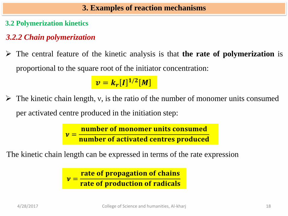
The central feature of the kinetic analysis is that the rate of polymerization is
proportional to the square root of the initiator concentration:
3. Examples of reaction mechanisms
3.2 Polymerization kinetics
3.2.2 Chain polymerization
𝒗 = 𝒌𝒓 𝑰𝟏/𝟐 𝑴
The kinetic chain length, ν, is the ratio of the number of monomer units consumed
per activated centre produced in the initiation step:
𝝂 =𝐧𝐮𝐦𝐛𝐞𝐫 𝐨𝐟 𝐦𝐨𝐧𝐨𝐦𝐞𝐫 𝐮𝐧𝐢𝐭𝐬 𝐜𝐨𝐧𝐬𝐮𝐦𝐞𝐝
𝐧𝐮𝐦𝐛𝐞𝐫 𝐨𝐟 𝐚𝐜𝐭𝐢𝐯𝐚𝐭𝐞𝐝 𝐜𝐞𝐧𝐭𝐫𝐞𝐬 𝐩𝐫𝐨𝐝𝐮𝐜𝐞𝐝
The kinetic chain length can be expressed in terms of the rate expression
𝝂 =𝐫𝐚𝐭𝐞 𝐨𝐟 𝐩𝐫𝐨𝐩𝐚𝐠𝐚𝐭𝐢𝐨𝐧 𝐨𝐟 𝐜𝐡𝐚𝐢𝐧𝐬
𝐫𝐚𝐭𝐞 𝐨𝐟 𝐩𝐫𝐨𝐝𝐮𝐜𝐭𝐢𝐨𝐧 𝐨𝐟 𝐫𝐚𝐝𝐢𝐜𝐚𝐥𝐬

4/28/2017 College of Science and humanities, Al-kharj 19
By making the steady-state approximation, we set the rate of production of radicals
equal to the termination rate
3. Examples of reaction mechanisms
3.2 Polymerization kinetics
3.2.2 Chain polymerization
𝜈 =𝑘𝑝 M• 𝑀
2𝑘𝑡.M 2 =𝑘𝑝 𝑀
2𝑘𝑡. M•
When we substitute the steady-state expression, for the radical concentration, we
obtain
𝝂 = 𝒌𝒓 𝑴 𝐈−𝟏/𝟐 𝒌𝒓 =
𝟏
𝟐𝒌𝒑(𝒇𝒌𝒊𝒌𝒕)
−𝟏/𝟐
4/28/2017 College of Science and humanities, Al-kharj 20
3. Examples of reaction mechanisms
3.2 Polymerization kinetics
3.2.2 Chain polymerization
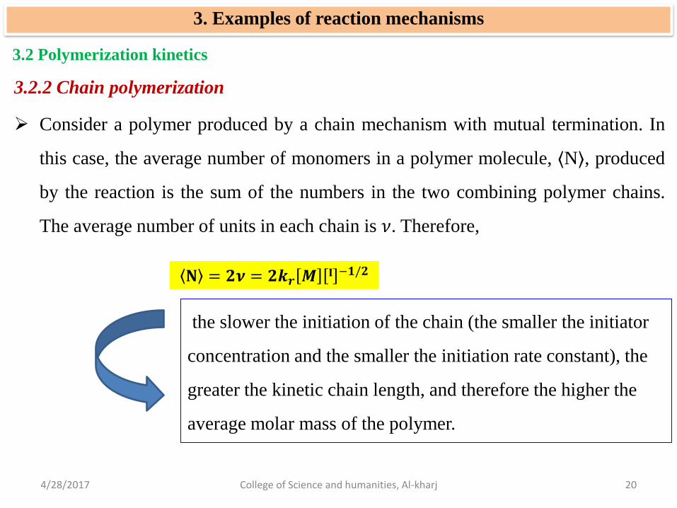
Consider a polymer produced by a chain mechanism with mutual termination. In
this case, the average number of monomers in a polymer molecule, ⟨N⟩, produced
by the reaction is the sum of the numbers in the two combining polymer chains.
The average number of units in each chain is 𝜈. Therefore,
𝐍 = 𝟐𝝂 = 𝟐𝒌𝒓 𝑴𝐈 −𝟏/𝟐
the slower the initiation of the chain (the smaller the initiator
concentration and the smaller the initiation rate constant), the
greater the kinetic chain length, and therefore the higher the
average molar mass of the polymer.

4/28/2017 College of Science and humanities, Al-kharj 21
3. Examples of reaction mechanisms
3.3 Phytochemistry
Many chemical reactions can be initiated (or started)
by the absorption of electromagnetic radiation.
In photochemical processes the radiant energy of the
Sun is absorbed (captured) by at least one
component of a reaction mixture.
Heating of the atmosphere during the daytime
by absorption of ultraviolet radiation.
The absorption of visible radiation during
photosynthesis.
Without photochemical processes, the Earth would
be simply a warm, sterile, rock.

4/28/2017 College of Science and humanities, Al-kharj 22
3. Examples of reaction mechanisms
3.3 Phytochemistry
Examples of photochemical processes

4/28/2017 College of Science and humanities, Al-kharj 23
3. Examples of reaction mechanisms
3.3 Phytochemistry
In a primary process, products are formed directly from the excited state of a
reactant.
Products of a secondary process originate from intermediates that are formed
directly from the excited state of a reactant.
Primary photophysical processes that can deactivate the excited state compete
with the formation of photochemical products.
Therefore, it is important to consider the timescales of excited state formation
and decay before describing the mechanisms of photochemical reactions.

4/28/2017 College of Science and humanities, Al-kharj 24
3. Examples of reaction mechanisms
3.3 Phytochemistry
Examples of photophysical processes

4/28/2017 College of Science and humanities, Al-kharj 25
Electronic transitions caused by absorption of ultraviolet and visible radiation
occur within 10−16–10−15 s.
Fluorescence is slower than absorption, with typical lifetimes of 10−12–10−6 s.
3. Examples of reaction mechanisms
3.3 Phytochemistry
We expect, then, that the upper limit for the rate constant of a first-
order photochemical reaction is about 1016 s−1.
The excited singlet state can initiate very fast photochemical reactions
in the femtosecond (10−15 s) to picosecond (10−12 s) timescale.
The initial events of vision
Photosynthesis
…
4/28/2017 College of Science and humanities, Al-kharj 26
3. Examples of reaction mechanisms
3.3 Phytochemistry
Typical intersystem crossing (ISC) and phosphorescence times for large organic
molecules are 10−12–10−4 s and 10−6–10−1 s, respectively.
Excited triplet states are photochemically important.
Because phosphorescence decay is several orders of magnitude slower than
most typical reactions, species in excited triplet states can undergo a very large
number of collisions with other reactants before deactivation.

4/28/2017 College of Science and humanities, Al-kharj 27
3. Examples of reaction mechanisms
3.3 Phytochemistry
3.3.1 The primary quantum yield
We shall see that the rates of deactivation of the excited state by radiative, non-
radiative, and chemical processes determine the yield of product in a
photochemical reaction.
The primary quantum yield, ∅
∅ =𝐧𝐮𝐦𝐛𝐞𝐫 𝐨𝐟 𝐞𝐯𝐞𝐧𝐭𝐬
𝐧𝐮𝐦𝐛𝐞𝐫 𝐨𝐟 𝐩𝐡𝐨𝐭𝐨𝐧𝐬 𝐚𝐛𝐬𝐨𝐫𝐛𝐞𝐝 When we divide both the
numerator and denominator
of ∅ by the time interval
over which the events
occurred ∅ =𝐫𝐚𝐭𝐞 𝐨𝐟 𝐩𝐫𝐨𝐜𝐞𝐬𝐬
𝐢𝐧𝐭𝐞𝐧𝐬𝐢𝐭𝐲 𝐨𝐟 𝐥𝐢𝐠𝐡𝐭 𝐚𝐛𝐬𝐨𝐫𝐛𝐞𝐝 =𝒗
𝐈𝐚𝐛𝐬
4/28/2017 College of Science and humanities, Al-kharj 28
3. Examples of reaction mechanisms
3.3 Phytochemistry
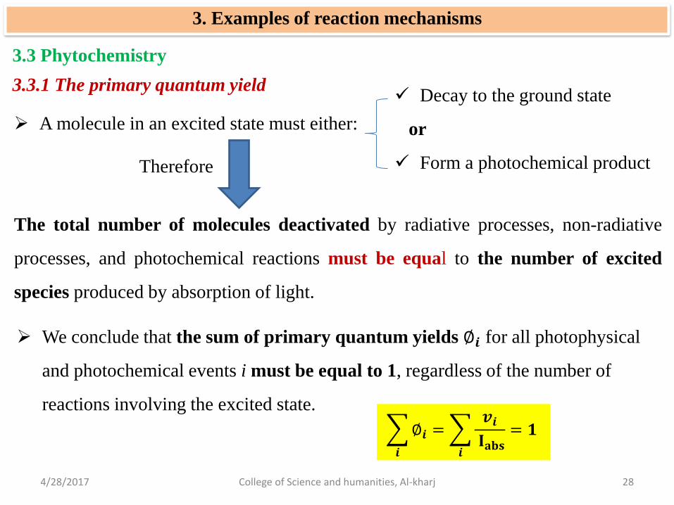
3.3.1 The primary quantum yield
A molecule in an excited state must either:
Decay to the ground state
or
Form a photochemical product
The total number of molecules deactivated by radiative processes, non-radiative
processes, and photochemical reactions must be equal to the number of excited
species produced by absorption of light.
Therefore
We conclude that the sum of primary quantum yields ∅𝒊 for all photophysical
and photochemical events i must be equal to 1, regardless of the number of
reactions involving the excited state.
∅𝒊𝒊
= 𝒗𝒊 𝐈𝐚𝐛𝐬𝒊
= 𝟏
4/28/2017 College of Science and humanities, Al-kharj 29
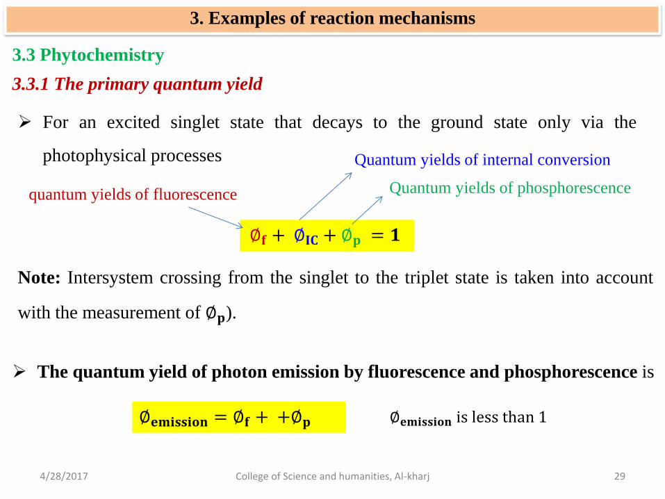
For an excited singlet state that decays to the ground state only via the
photophysical processes
3. Examples of reaction mechanisms
3.3 Phytochemistry
3.3.1 The primary quantum yield
∅𝐟 + ∅𝐈𝐂 + ∅𝐩 = 𝟏
Note: Intersystem crossing from the singlet to the triplet state is taken into account
with the measurement of ∅𝐩).
quantum yields of fluorescence
Quantum yields of internal conversion
Quantum yields of phosphorescence
The quantum yield of photon emission by fluorescence and phosphorescence is
∅𝐞𝐦𝐢𝐬𝐬𝐢𝐨𝐧 = ∅𝐟 + +∅𝐩 ∅𝐞𝐦𝐢𝐬𝐬𝐢𝐨𝐧 is less than 1

4/28/2017 College of Science and humanities, Al-kharj 30
If the excited singlet state also participates in a primary photochemical reaction
with quantum yield ∅𝒓, we write:
3. Examples of reaction mechanisms
3.3 Phytochemistry
3.3.1 The primary quantum yield
∅𝐟 + ∅𝐈𝐂 + ∅𝐩 + ∅𝐫 = 𝟏
We can now strengthen the link between reaction rates and primary quantum yield
∅ =𝒗
𝒗𝒊𝒊
𝑣𝑖𝑖
= Iabs and ∅ =𝒗
𝐈𝐚𝐛𝐬
The primary quantum yield may be determined
directly from the experimental rates of all
photophysical and photochemical processes that
deactivate the excited state.
Therefore

4/28/2017 College of Science and humanities, Al-kharj 31
3. Examples of reaction mechanisms
3.3 Phytochemistry
3.3.2 Mechanism of decay of excited singlet states
Consider the formation and decay of an excited singlet state in the absence of a
chemical reaction:
Absorption: S + hνi → S∗ 𝑣𝑎𝑏𝑠 = Iabs
Fluorescence: S∗ → S + +hνf 𝑣𝑓 = kf S∗
Internal conversion: S∗ → S 𝑣𝐼𝐶 = kIC S∗
Intersystem crossing: S∗ → T∗ 𝑣𝐼𝑆𝐶 = kISC S∗
Absorbing species Excisted singlet state
Excisted triplet state
Energy of incident photons
Energy of fluorescent photons
𝐑𝐚𝐭𝐞 𝐨𝐟 𝐟𝐨𝐫𝐦𝐚𝐭𝐢𝐨𝐧 𝐨𝐟 𝑺∗ = Iabs
𝐑𝐚𝐭𝐞 𝐨𝐟 𝐝𝐞𝐜𝐚𝐲 𝐨𝐟 𝑺∗ = − kf S∗ − kIC S
∗ − kISC S∗ = −(kf + kISC + kIC) S
∗

4/28/2017 College of Science and humanities, Al-kharj 32
It follows that the excited state decays
by a first-order process so, when the
light is turned off, the concentration of
S* varies with time t as:
3. Examples of reaction mechanisms
3.3 Phytochemistry
3.3.2 Mechanism of decay of excited singlet states
S + hνi → S∗ 𝑣𝑎𝑏𝑠 = Iabs
S∗ → S + +hνf 𝑣𝑓 = kf S∗
S∗ → S 𝑣𝐼𝐶 = kIC S∗
S∗ → T∗ 𝑣𝐼𝑆𝐶 = kISC S∗
𝐑𝐚𝐭𝐞 𝐨𝐟 𝐟𝐨𝐫𝐦𝐚𝐭𝐢𝐨𝐧 𝐨𝐟 𝑺∗
= Iabs
𝐑𝐚𝐭𝐞 𝐨𝐟 𝐝𝐞𝐜𝐚𝐲 𝐨𝐟 𝑺∗
= −(kf + kISC + kIC) S∗
𝐒∗ 𝐭 = 𝐒∗𝟎𝐞−𝐭/𝛕𝟎
The observed lifetime, τ0, of
the first excited singlet state 𝛕𝟎 =
𝟏
𝐤𝐟 + 𝐤𝐈𝐒𝐂 + 𝐤𝐈𝐂
The quantum yield of fluorescence (Justify) is
𝛟𝐟 = 𝐤𝐟
𝐤𝐟 + 𝐤𝐈𝐒𝐂 + 𝐤𝐈𝐂

4/28/2017 College of Science and humanities, Al-kharj 33
3. Examples of reaction mechanisms
3.3 Phytochemistry
3.3.2 Mechanism of decay of excited singlet states 𝛕𝟎 = 𝟏
𝐤𝐟 + 𝐤𝐈𝐒𝐂 + 𝐤𝐈𝐂
The observed fluorescence lifetime, 𝛕𝟎 can be measured by using a pulsed laser
technique.
First, the sample is excited with a short light pulse from a laser using a
wavelength at which S absorbs strongly.
Then, the exponential decay of the fluorescence intensity after the pulse is
monitored. it follows that
𝛕𝟎 = 𝟏
𝐤𝐟 + 𝐤𝐈𝐒𝐂 + 𝐤𝐈𝐂=
𝐤𝐟𝐤𝐟 + 𝐤𝐈𝐒𝐂 + 𝐤𝐈𝐂
×𝟏
𝐤𝐟=𝛟𝐟𝐤𝐟

4/28/2017 College of Science and humanities, Al-kharj 34
3. Examples of reaction mechanisms
3.3 Phytochemistry
3.3.2 Mechanism of decay of excited singlet states
Example:
In water, the fluorescence quantum yield and observed fluorescence lifetime of
tryptophan are ϕf = 0.20 and τ0 = 2.6 ns, respectively.
It follows that the fluorescence rate constant kf is
τ0 = ϕfkf =
0.20
2.6 × 10⁻⁹s = 7.7 × 10⁷ s−1
4/28/2017 College of Science and humanities, Al-kharj 35
3. Examples of reaction mechanisms
3.3 Phytochemistry
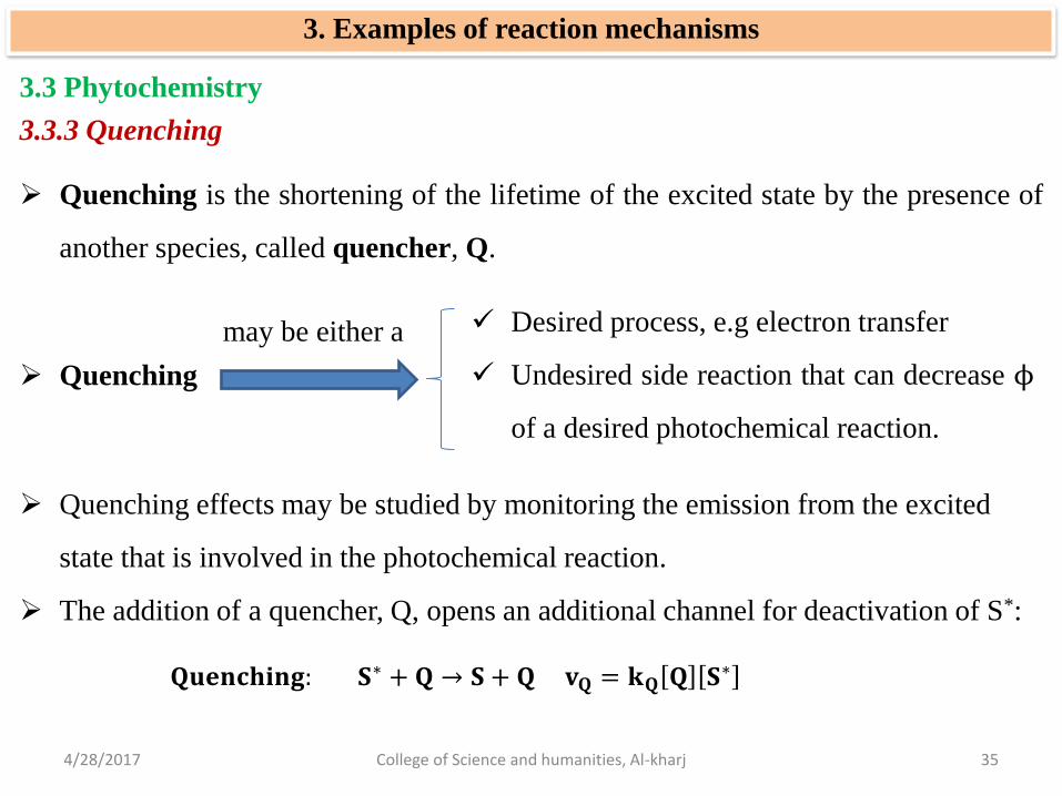
3.3.3 Quenching
Quenching is the shortening of the lifetime of the excited state by the presence of
another species, called quencher, Q.
Quenching
Desired process, e.g electron transfer
Undesired side reaction that can decrease ϕ
of a desired photochemical reaction.
Quenching effects may be studied by monitoring the emission from the excited
state that is involved in the photochemical reaction.
The addition of a quencher, Q, opens an additional channel for deactivation of S*:
may be either a
𝐐𝐮𝐞𝐧𝐜𝐡𝐢𝐧𝐠: 𝐒∗ + 𝐐 → 𝐒 + 𝐐 𝐯𝐐 = 𝐤𝐐 𝐐 𝐒∗
4/28/2017 College of Science and humanities, Al-kharj 36
3. Examples of reaction mechanisms
3.3 Phytochemistry
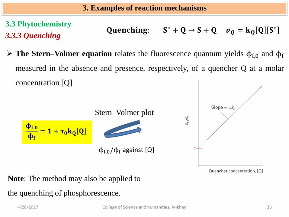
3.3.3 Quenching 𝐐𝐮𝐞𝐧𝐜𝐡𝐢𝐧𝐠: 𝐒∗ + 𝐐 → 𝐒 + 𝐐 𝒗𝑸 = 𝐤𝐐 𝐐 𝐒
∗
The Stern–Volmer equation relates the fluorescence quantum yields ϕf,0 and ϕf
measured in the absence and presence, respectively, of a quencher Q at a molar
concentration [Q]
𝛟𝐟,𝟎𝛟𝐟= 𝟏 + 𝛕𝟎𝐤𝐐 𝐐
Stern–Volmer plot
ϕf,0/ϕf against [Q]
Note: The method may also be applied to
the quenching of phosphorescence.
4/28/2017 College of Science and humanities, Al-kharj 37
3. Examples of reaction mechanisms
3.3 Phytochemistry
3.3.3 Quenching
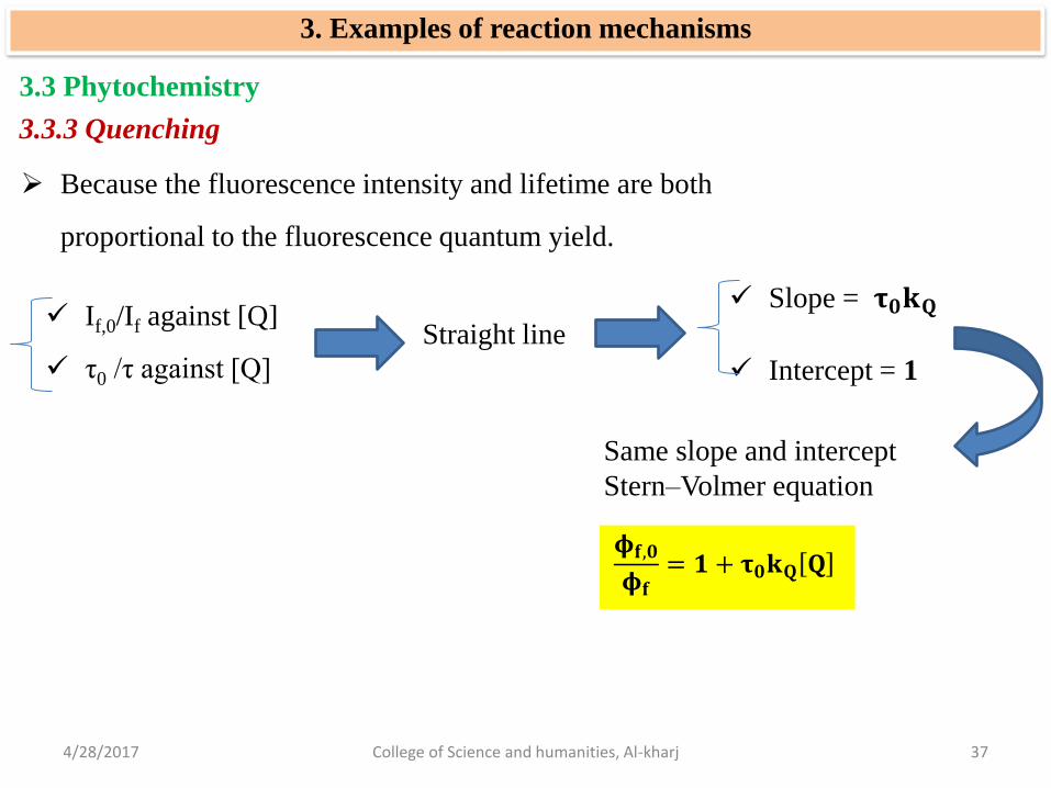
Because the fluorescence intensity and lifetime are both
proportional to the fluorescence quantum yield.
If,0/If against [Q]
τ0 /τ against [Q] Straight line
Slope = 𝛕𝟎𝐤𝐐
Intercept = 1
Same slope and intercept
Stern–Volmer equation
𝛟𝐟,𝟎𝛟𝐟= 𝟏 + 𝛕𝟎𝐤𝐐 𝐐

4/28/2017 College of Science and humanities, Al-kharj 38
3. Examples of reaction mechanisms
3.3 Phytochemistry
3.3.3 Quenching
Example: Determining the quenching rate constant
2,2′-bipyridine (1, bpy) forms a complex with the Ru2+ ion.
Ruthenium (II) tris-(2,2′-bipyridyl), Ru(bpy)3 2+ (2), has a strong
metal-to-ligand charge transfer (MLCT) transition at 450 nm.
The quenching of the *Ru(bpy)3 2+ excited state by Fe(OH2)6
3+ in
acidic solution was monitored by measuring emission lifetimes at
600 nm. Determine the quenching rate constant for this reaction
from the following data:
[Fe(OH2)6 3+]/(10−4 mol dm−3) 0 1.6 4.7 7 9.4
τ /(10−7 s) 6 4.05 3.37 2.96 2.17
Solution (word file p. 62)

4/28/2017 College of Science and humanities, Al-kharj 39
3. Examples of reaction mechanisms
3.3 Phytochemistry
3.3.3 Quenching
Three common mechanisms for bimolecular quenching of an excited singlet (or
triplet) state are proposed:
Collisional deactivation: S* + Q→S + Q
Resonance energy transfer: S* + Q→ S + Q*
Electron transfer: S* + Q→ S+ + Q− or S− + Q+
Note: The quenching rate constant itself does not give much insight into the
mechanism of quenching.
There are some criteria that govern the relative efficiencies of collisional
quenching, energy transfer, and electron transfer.

4/28/2017 College of Science and humanities, Al-kharj 40
3. Examples of reaction mechanisms
3.3 Phytochemistry
3.3.3 Quenching
There are some criteria that govern the relative efficiencies of collisional
quenching, energy transfer, and electron transfer.
Collisional deactivation: S* + Q→S + Q
Resonance energy transfer: S* + Q→ S + Q*
Electron transfer: S* + Q→ S+ + Q− or S− + Q+
Collisional quenching is particularly efficient when Q is a heavy species (e.g.,
iodide ion), which receives energy from S* and then decays primarily by internal
conversion to the ground state.

4/28/2017 College of Science and humanities, Al-kharj 41
According to the Marcus theory of electron transfer, the rates of electron transfer
(from ground or excited states) depend on:
The distance between the donor and acceptor, with electron transfer
becoming more efficient as the distance between donor and acceptor
decreases.
The reaction Gibbs energy, ΔrG, with electron transfer becoming more
efficient as the reaction becomes more exergonic (e.g., efficient
photooxidation of S requires that the reduction potential of S* be lower than
the reduction potential of Q).
3. Examples of reaction mechanisms
3.3 Phytochemistry
3.3.3 Quenching

4/28/2017 College of Science and humanities, Al-kharj 42
3. Examples of reaction mechanisms
3.3 Phytochemistry
3.3.3 Quenching
The reorganization energy, the energy cost incurred by molecular
rearrangements of donor, acceptor, and medium during electron transfer.
The electron transfer rate is predicted to increase as this reorganization
energy is matched closely by the reaction Gibbs energy.
According to the Marcus theory of electron transfer, the rates of electron transfer
(from ground or excited states) depend on:
Electron transfer can also be studied by time-resolved spectroscopy. The
oxidized and reduced products often have electronic absorption spectra distinct
from those of their neutral parent compounds. Therefore, the rapid appearance of
such known features in the absorption spectrum after excitation by a laser pulse
may be taken as indication of quenching by electron transfer. In the following
section we explore energy transfer in detail.
4/28/2017 College of Science and humanities, Al-kharj 43
3. Examples of reaction mechanisms
3.3 Phytochemistry
3.3.3 Quenching
Electron transfer can also be studied by time-resolved spectroscopy.
The oxidized and reduced products often have electronic absorption spectra
distinct from those of their neutral parent compounds. Therefore, the rapid
appearance of such known features in the absorption spectrum after excitation by
a laser pulse may be taken as indication of quenching by electron transfer.

4/28/2017 College of Science and humanities, Al-kharj 44
3. Examples of reaction mechanisms
3.3 Phytochemistry
3.3.4 Resonance energy transfer
We visualize the process S* + Q → S + Q* as follows:
The oscillating electric field of the incoming electromagnetic radiation
induces an oscillating electric dipole moment in S.
Energy is absorbed by S if the frequency of the incident radiation, ν, is such
that ν = ΔES/h, where ΔES is the energy separation between the ground and
excited electronic states of S and h is Planck’s constant.
=> This is the ‘resonance condition’ for absorption of radiation.
The oscillating dipole on S now can affect electrons bound to a nearby Q molecule
by inducing an oscillating dipole moment in the latter. If the frequency of
oscillation of the electric dipole moment in S is such that ν =ΔEQ/h then Q will
absorb energy from S. The efficiency, ηT, of resonance energy transfer is defined
as

4/28/2017 College of Science and humanities, Al-kharj 45
3. Examples of reaction mechanisms
3.3 Phytochemistry
3.3.4 Resonance energy transfer
If the frequency of oscillation of the electric dipole moment in S is such that
ν =ΔEQ/h
then Q will absorb energy from S.
𝜼𝑻 = 𝟏 −𝝓𝒇
𝝓𝒇,𝟎
According to the Förster theory of resonance energy transfer, energy transfer is
efficient when:
The energy donor and acceptor are separated by a short distance (of the order
of nanometres).
Photons emitted by the excited state of the donor can be absorbed directly by
the acceptor.
The efficiency, ηT, of resonance energy transfer is defined as

4/28/2017 College of Science and humanities, Al-kharj 46
3. Examples of reaction mechanisms
3.3 Phytochemistry
3.3.4 Resonance energy transfer
For donor–acceptor systems that are held rigidly either by
covalent bonds or by a protein ‘scaffold’, ηT increases with
decreasing distance, R.
𝛈𝐓 =𝐑𝟎𝟔
𝐑𝟎𝟔 + 𝐑𝟔
Is a parameter (with units of distance) that
is characteristic of each donor–acceptor
pair

4/28/2017 College of Science and humanities, Al-kharj 47
3. Examples of reaction mechanisms
3.3 Phytochemistry
3.3.4 Resonance energy transfer
The emission and absorption spectra of
molecules span a range of wavelengths, so
the second requirement of the Förster
theory is met when the emission spectrum
of the donor molecule overlaps significantly
with the absorption spectrum of the
acceptor.
In the overlap region, photons emitted by
the donor have the proper energy to be
absorbed by the acceptor.
4/28/2017 College of Science and humanities, Al-kharj 48
3. Examples of reaction mechanisms
3.3 Phytochemistry
3.3.4 Resonance energy transfer
In many cases, the energy transfer is the predominant mechanism of quenching if
the excited state of the acceptor fluoresces or phosphoresces at a characteristic
wavelength.
In a pulsed laser experiment, the rise in fluorescence intensity from Q* with a
characteristic time that is the same as that for the decay of the fluorescence of S* is
often taken as indication of energy transfer from S to Q.
𝛈𝐓 =𝐑𝟎𝟔
𝐑𝟎𝟔 + 𝐑𝟔
forms the basis of fluorescence resonance energy transfer
(FRET), in which the dependence of the energy transfer
efficiency, ηT, on the distance, R, between energy donor and
acceptor can be used to measure distances in biological
systems.
4/28/2017 College of Science and humanities, Al-kharj 49
3. Examples of reaction mechanisms
3.3 Phytochemistry
3.3.4 Resonance energy transfer
In a typical FRET experiment, a site on a biopolymer or membrane is labelled
covalently with an energy donor and another site is labelled covalently with an
energy acceptor.
In certain cases, the donor or acceptor may be natural constituents of the system,
such as amino acid groups, co-factors, or enzyme substrates.
The distance between the labels is then calculated from the known value of R0 and
the equation:
Several tests have shown that the FRET technique is useful for measuring
distances ranging from 1 to 9 nm.
𝛈𝐓 =𝐑𝟎𝟔
𝐑𝟎𝟔 + 𝐑𝟔

4/28/2017 College of Science and humanities, Al-kharj 50
3. Examples of reaction mechanisms
3.3 Phytochemistry
3.3.4 Resonance energy transfer
Brief illustration
Consider a study of the protein rhodopsin. When an amino
acid on the surface of rhodopsin was labelled covalently
with the energy donor 1.5-I AEDANS, the fluorescence
quantum yield of the label decreased from 0.75 to 0.68 due
to quenching by the visual pigment 11-cis-retinal.
ηT = 1 − (0.68/0.75) = 0.093
From the known value of R0 = 5.4 nm for the 1.5-I
AEDANS/11-cis-retinal pair => R = 7.9 nm
Therefore, we take 7.9 nm to be the distance between the
surface of the protein and 11-cis-retinal.

4/28/2017 College of Science and humanities, Al-kharj 51
3. Examples of reaction mechanisms
3.3 Phytochemistry
3.3.4 Resonance energy transfer
If donor and acceptor molecules diffuse in solution or in the gas phase, Förster
theory predicts that the efficiency of quenching by energy transfer increases as the
average distance travelled between collisions of donor and acceptor decreases.
That is, the quenching efficiency increases with concentration of quencher, as
predicted by the Stern–Volmer equation.
Thank you for your presence and intention
& Many thanks to P. Atkins, J. D Paula for
their nice book “ Physical chemistry”