physical and computational studies of slag …
TRANSCRIPT

PHYSICAL AND COMPUTATIONAL STUDIES
OF SLAG BEHAVIOR IN AN ENTRAINED
FLOW GASIFIER
by
Randy Pummill
A dissertation submitted to the faculty of
The University of Utah
in partial fulfillment of the requirements for the degree of
Doctor of Philosophy
Department of Chemical Engineering
The University of Utah
August 2012

Copyright © Randy Pummill 2012
All Rights Reserved

T h e U n i v e r s i t y o f U t a h G r a d u a t e S c h o o l
STATEMENT OF DISSERTATION APPROVAL
The dissertation of Randy Pummill
has been approved by the following supervisory committee members:
Kevin Whitty , Chair 6/8/2012
Date Approved
Eric Eddings , Member 6/8/2012
Date Approved
Thomas Fletcher , Member 6/11/2012
Date Approved
Robert Stoll , Member 6/8/2012
Date Approved
Constance Senior , Member 6/8/2012
Date Approved
and by JoAnn Lighty , Chair of
the Department of Chemical Engineering
and by Charles A. Wight, Dean of The Graduate School.

ABSTRACT
This work details an investigation of how to modify slag flow so as to maintain a
clear line of sight across the reaction section of an entrained-flow coal gasifier. Physical
and computational models were developed to study methods of diverting the molten slag
that flows vertically down the walls of the reactor. The physical models employed
silicone oil of varying viscosity. The computational models were developed using the
Fluent software package. Based on the insight gained from the results of the models, two
devices were created and tested in a pilot scale gasifier located at the University of Utah.
The first method of slag diversion studied employed a gas jet to impact the slag
film and cause it to flow around a sight port in the gasifier wall. By studying the film and
jet interactions, it was discovered that the resulting behavior of such a system can be
described by a dimensionless ratio of the kinetic energy of the jet and the surface energy
of the film. The development of the dimensionless number, called a Lotte number in this
work, is presented in detail. Generally, viscous films will be broken by a jet when the
Lotte number is greater than 5 and will reclose when the Lotte number falls below a value
of 1.5.
The second slag diversion method studied used a round alumina tube protruding
horizontally into the reaction section to break up the film. As the film impacts the tube, it
progresses horizontally along the length of the tube before resuming the downward flow.

iv
The models helped to establish how far the tube should protrude into the reactor in order
to successfully break up the slag flow.
Slag diversion devices were constructed and installed on a pilot scale gasifier.
The jet diversion method was found to require an unreasonably large amount of purge gas
to be successful and the metal jet suffered from the high temperature of the reactor
despite the cooling effect of the gas. The tube diversion method worked very well for a
series of experiments. However, erosion of the alumina tube in the reaction section
remains an impediment to using such a device in an industrial setting. A design using a
water-cooled tube is suggested.

To Rachel, my wonderful partner and friend and our four terrible, funny, and
delightful children

CONTENTS
ABSTRACT ……………………………………………………………………………. iii
LIST OF FIGURES …………………………………………………………………….viii
LIST OF TABLES …………………………………………………………………….... xi
ACKNOWLEDGEMENTS ……………………………………………………………. xii
Chapter
1 INTRODUCTION ………………………………………………………………. 1
1.1 Gasification ………………………………………………………………….. 1
1.2 Research Motivation ………………………………………………………… 4
2 REVIEW OF LITERATURE ………………………………………………….... 6
2.1 Slag Formation and Structure ………..……………………………………… 6
2.2 Temperature/Viscosity Relationships …………………………..…………… 9
2.3 Other Slag Property Studies ………………………………………...……… 23
2.4 Computational Modeling of Slag in a Reactor ………………………….….. 27
2.5 Jet Impinging on Thin Film Studies ………………………………….…….. 30
2.6 Summary ……………………………………………………......................... 31
3 OBJECTIVE AND APPROACH ……………...…………...………………...... 33
3.1 Objective…………………………………………………………..………... 33
3.2 Proposed Methods ………………………………………………..……….... 34
3.3 Approach …………………………………………………………………… 36
4 EXPERIMENTAL ……………………………………………….…………….. 38
4.1 Introduction .…………………………………………………..……………. 38
4.2 Silicone Oil Model .………………………………………………………… 38
4.3 Computational Model ………………………………………………………. 53
4.4 Gasifier Application …………………………………………….………..… 68
vii
5 RESULTS AND DISCUSSION ……………………………………………….. 81
5.1 Silicone Oil Experiments ……………………………………….…..................... 81
5.2 Computational Experiments …………………........……………...……….. 103
5.3 Gasifier Application ………………………………………………………. 125
6 SUMMARY AND CONCLUSIONS ………………………………………… 135
APPENDICES
A: FALLING FILM THICKNESS CALCULATION ………………………. 139
B: MAXIMUM SHEAR RATE OF SILICONE OIL ……………………….. 145
C: SLAG VISCOSITY MODEL IN UDF FORM …………………………… 148
D: PENDANT DROP METHOD ……………………………………………. 149
E: GASIFIER FEED RATE EQUATION ………………………………..….. 153
REFERENCES ……………………………………………………………………….. 155

LIST OF FIGURES
Figure
2.1 Illustration of temperature of critical viscosity …..…………………………….. 10
2.2 Glassy and crystalline slag viscosity versus temperature …...…………………. 12
3.1 Diagram of jet diversion method ………………………………………………. 35
4.1 Schematic of physical model setup ………………………………………….…. 40
4.2 Wall geometry for oil tests …………………………………………………….. 41
4.3 Jet impingement angle measurement …………………………………………... 42
4.4 Tube within elliptical slot …………………………………………………….... 43
4.5 Dimensions of refractory cast ………………………………………………….. 45
4.6 Structure of polydimethylsiloxane ……………………………………………... 47
4.7 Pendant droplet technique for measuring surface tension ……………………... 47
4.8 Silicone oil on impact with the tube …………………………………………… 51
4.9 Geometry for impinging jet computational model ……………………………... 55
4.10 Detail of hole and tube …………………………………………………………. 56
4.11 Top boundary arrangement of slag inlet boundary …………………………….. 57
4.12 Tube diversion computational model geometry ……………………………….. 59
4.13 Geometry wireframe front view ……………………………………………….. 61
4.14 Geometry wireframe isometric view …………………………………………... 62
4.15 Slag viscosity experimental data versus model predictions ……………………. 67

ix
4.16 Cut-away section of the gasifier ……………………………………………….. 70
4.17 Jet diversion device ………………………………………………………..…… 72
4.18 Optical access window design …………………………………………………. 73
4.19 Steel window holders with sapphire pieces ……………………………………. 75
4.20 Assembled alumina tube diversion device ……………………………………... 76
4.21 Retaining ring of tube diversion device ………………………………………... 76
4.22 Window assembly of tube diversion device ………………………………….... 77
4.23 Mounted assembly of tube diversion device …………………………………… 78
5.1 Low flow rate jet and silicone oil film …………………………………………. 82
5.2 Increased flow rate with larger oil bubble ……………………………………... 83
5.3 Increased flow rate with fluctuating bubble …………………………………… 84
5.4 Silicone oil hood formation ……………………………………………………. 85
5.5 Reformed oil bubble …………………………………………………………… 88
5.6 Jet mass flow rate data for film burst ………………...……………………….... 95
5.7 Lotte number versus impingement angle for film burst ………………...……… 96
5.8 Jet mass flow rate for film closure …………………………………………...… 98
5.9 Lotte number for film closure ………………………………………………..… 98
5.10 Jet flow rate versus film thickness for burst and closure ……………………... 100
5.11 Lotte number versus film thickness for burst and closure ……………………. 100
5.12 Tube length versus oil flow rate …………………………………….………… 102
5.13 Jet diversion model at low Lotte number ……………………………………... 104
5.14 Jet diversion for Lo = 8.0 ……………………………………………………... 106
5.15 Jet diversion results for high film flow rate, Lo = 8.0 ………………………... 107

x
5.16 Jet diversion results for high film flow rate, Lo = 13.5 ………………………. 108
5.17 Baseline simulation results at 250 time steps ………………………………… 111
5.18 Baseline simulation results at 500 time steps ………………………………… 113
5.19 Baseline simulation results at 500 time steps, side view ……………………... 114
5.20 Baseline simulation results at 750 time steps ………………………………… 115
5.21 Baseline simulation results at 750 time steps, side view ……………………... 116
5.22 Variable jet flow rate simulation results ……………………………………… 117
5.23 Variable jet temperature simulation results …………………………………... 119
5.24 First tube simulation results …………………………………………………... 122
5.25 Second tube simulation results ………………………………………………... 123
5.26 Third tube simulation results ………………………………………………..... 124
5.27 Jet diversion device after use in gasifier ……………………………………… 128
5.28 Sight port after jet diversion experiments …………………………………….. 129
5.29 Alumina tube and slag in the gasifier ………………………………………… 132
5.30 Cracked alumina tube in the gasifier …………………………………………. 133
5.31 Recovered alumina tube from gasifier experiments ………………………….. 135
A.1 Momentum fluxes …………………………………………………………….. 140
D.1 Surface tension measuring device …………………………………………….. 151
D.2 Droplet chamber with suspended droplet …………………………………….. 152

LIST OF TABLES
Table
2.1 Summary of mineral matter present in coal …..…………………………………. 7
2.2 Fitted values for bi ……………………………………………………………… 19
4.1 Silicone oil properties ....……………………………………………………….. 48
4.2 Ash composition in weight percentage of Sufco coal ………………………….. 64
4.3 Under-relaxation factors for computational model …………………………….. 68
4.5 Ultimate analysis of Skyline and Sufco coals ………………………………….. 79
4.6 Proximate analysis of Skyline and Sufco coals ………………………………... 79
4.7 Ash composition analysis of Skyline and Sufco coals …………………………. 80
5.1 Tube diversion results ………………………………………………………… 102
5.2 Conditions for jet diversion simulations ……………………………………… 110
5.3 Conditions for tube diversion simulations ……………………………………. 121
B.1 Critical shear rates for silicone oil ……………………………………………. 145
B.2 Calculated critical shear rates ………………………………………………… 145
B.3 Critical shear rates and maximum shear rates ………………………………… 147

ACKNOWLEDGEMENTS
As with any accomplishment, this work is truly the result of the efforts of many
people. The author wishes to thank the many people who have lent their time and talents.
Thanks to Eric Berg, Mike Burton, Gabe Hansen, David Ray Wagner, Travis
Waind, and Dan Sweeney for their help with developing the physical model and in
operating the gasifier.
Thanks to Kevin Whitty and Dave Wagner for all their advice and guidance. It
surely saved my life more than once. Thanks to Robin Hughes for helping me to
understand that sometimes a simple solution is best. Thanks also to Jay Jeffries, Kai Sun,
Ritobrata Sur, and Stanford University for the opportunity to work on this project. It was
a pleasure. Thanks also to my committee for their advice and valuable feedback during
this project.
And finally, thanks to my wife and family for their patience and steadfast support.
This work was supported by a U.S. Department of Energy Cooperative
Agreement via Stanford University, DE-FE0001180.

CHAPTER 1
INTRODUCTION
1.1 Gasification
Coal gasification is a chemical process similar to combustion. In both processes,
the coal is oxidized and gives off useful heat. During the combustion of coal, the carbon
and hydrogen present in the coal reacts with oxygen from an air feed. The amount of
oxygen fed is enough to completely react with all of the available carbon and hydrogen.
This reaction produces carbon dioxide and water as the major products, as seen in
Equation 1.1:
(1.1)
In contrast, gasification is usually carried out with a pure oxygen feed instead of
an air feed. In gasification, the oxygen is fed in substoichiometric amounts so that the
major product of the reaction is a mixture of hydrogen and carbon monoxide gas, as
shown in Equation 1.2. This product gas is often called syngas, as it can be used to
synthesize a great many other useful chemicals or used directly in gas turbine to produce
electrical power.
(1.2)

2
Carbon-based fuel gasification is a very old technology, but, despite its age, its
use for electricity production is still relatively new. Only a small number of integrated
gasification combined cycle (IGCC) power plants are operating today. Historically, the
syngas product has had many uses. Coal gas or town gas was produced via coal
gasification in the United States and Europe. The gas was primarily used for streetlights
and home heating before the Second World War; its use died out as natural gas gained
infrastructure and popularity (Everard, 1949). From the 1940s to the present, coal
gasification has been used to create liquid fuels. In his review, Dry (1996) notes that this
is done by converting the syngas to petroleum substitutes via Fischer-Tropsch reactions.
More recently, coal gasification has been investigated as a possible power source via
Integrated Gasification Combined-cycle (IGCC) systems.
The thermodynamic cycles of an IGCC system are much more efficient than those
of a standard coal combustion system. For example, Beér (2007) estimates that while a
coal combustion-based, steam-generator electrical plant will have an efficiency rate of
32%, a gasification-based electrical plant is estimated to be about 47% efficient.
Coal gasifiers operate at elevated temperatures. Steels are not able to withstand
such excessive temperatures and so any gasification reactor must either be insulated or
actively cooled while running. The reactor at the University of Utah Advanced
Gasification Research Center that was used for this project relies on insulation, with thick
pieces of refractory lining the interior of the reactor walls. The refractory is designed so
that the reactor shell temperature is maintained below 530 K during operation.

3
Gasification also varies from combustion in the area of operating pressure. Most
common combustion processes are performed at pressures just under that of the ambient
environment. This ensures that the reactants and products will not leak out of the
reaction areas. Gasification is generally performed at high pressures, between 30 and 70
bar. The high pressure allows gasification reactors to be compact when compared to
combustion reactors of similar energy output, and increases process efficiency,
particularly in the clean up and mercury removal phases. Beér (2007) also notes that the
high outlet pressure also lends an overall efficiency advantage when carbon sequestration
is considered.
Overall, gasification offers many advantages over traditional coal combustion as
an energy source but has yet to be fully embraced by utility companies. This reluctance
is mostly due high capital and research costs and to uncertainties about how the process
and facilities will fare in the long term. Most of the long term data on the gasification
process has been collected by private companies and is proprietary.
To bring this information into the public sphere and encourage adoption of the
technology, the U.S. Department of Energy has made many efforts to fund research
projects to increase the viability and attractiveness of coal gasification as a source of
electrical energy production. One example is the TECO Polk Power Station located in
Polk County, Florida, USA. This plant represents a joint effort between TECO and the
U.S. government, which contributed $120 million to the project (TECO Energy 2012).
The 250 MW plant began operation in 1997 uses an IGCC to maximize efficiency. It has
been in full-scale, commercial operation since 2002 (McDaniel 2002).

4
Despite the efforts of the U.S. Department of Energy, industry as a whole has
been slow to embrace gasification. In their report to the U.S. Department of Energy,
Clayton et al. (2002) identified many possible areas for improvement to motivate large
scale adoption of gasification technology. This list included better injector design, fuel
flexibility, refractory wear and improvement studies, slag removal techniques, and
instrumentation. Improving these areas will result in increased confidence in gasification
technology and could lead to wider adoption of the technology.
1.2 Research Motivation
Fast and reliable instrumentation has been identified as a critical need for
gasification technology (Clayton et al. 2002). The aggressive environment inside a high-
temperature, slagging gasification reactor can make getting reliable temperature and gas
composition data from the reactor very difficult. Any physical probes used to obtain data
are subject to the extremely high temperatures and the reducing environment of the
reactor and will consequently have a very short lifetime.
One way to overcome this limitation is to use a noninvasive measuring device
such as an optically-based measurement system. Work by Sanders et al. (2001), Zhou et
al. (2003), Jeffries (2009), and Ortwein et al. (2010) has shown that by directing a tunable
laser through the hot gases inside the reactor and measuring the absorbance spectra at
different wavelengths, data such as temperature and major species concentrations can be
obtained. In order to function properly, such a measurement device would require a clear
line of sight across the entire reactor.
One impediment to an optically-based system is layer of slag on the reactor walls.
As coal particles react, much of the mineral matter present in the coal remains as ash.

5
The amount of ash depends on the coal’s origin but is often a significant portion of the
original coal mass, generally making up more than 20% of the mass of the coal. In a
gasification environment, the high temperatures cause the ash to become molten, which is
then called slag. The molten slag will stick to the walls of the reactor and, over time, will
accumulate and flow downward. This slag flow would likely flow over any sight ports
cut into the reactor refractory and interfere with the line of sight necessary for the laser
measurements.

CHAPTER 2
REVIEW OF LITERATURE
2.1 Slag Formation and Structure
Slag is crystalline mineral matter in either the molten or solid form and is the
byproduct of many processes including coal combustion, coal gasification, and steel
manufacturing. In solid form, slag is a brittle crystalline structure with dark coloration.
Slag often contains entrapped bubbles of gas. These bubbles are entrapped while the slag
is in molten liquid form and fixed in place as the slag cools. This gas generally consists
of hydrogen, nitrogen, and carbon monoxide which are in high concentration during the
gasification process.
Slag consists of the residual mineral matter from the coal after the more volatile
chemicals have been consumed. From the work done by Smith et al. (1994), of the
standard Argonne coals analyzed, the mineral matter present ranged from 4.6% to 29.6%
on a dry, sulfur free basis. This mineral matter predominantly consists of silicon,
aluminum, calcium, and iron oxides in majority, and some trace amounts of other
minerals and metals such as titanium, potassium, magnesium, sodium, and phosphorus.
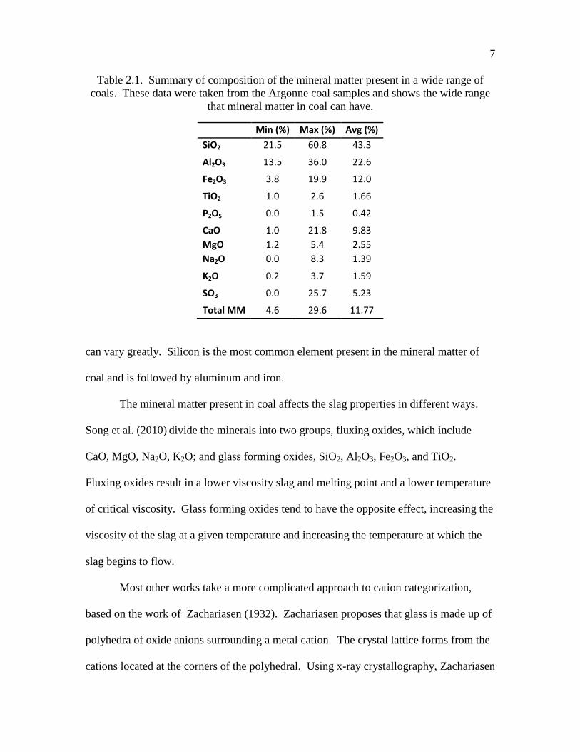
Table 2.1 gives information on mineral matter in various coals from the Argonne
coal depository (Smith et al. 1994). As can be observed, the amount of mineral in coal
7
Table 2.1. Summary of composition of the mineral matter present in a wide range of
coals. These data were taken from the Argonne coal samples and shows the wide range
that mineral matter in coal can have.
Min (%) Max (%) Avg (%)
SiO2 21.5 60.8 43.3
Al2O3 13.5 36.0 22.6
Fe2O3 3.8 19.9 12.0
TiO2 1.0 2.6 1.66
P2O5 0.0 1.5 0.42
CaO 1.0 21.8 9.83
MgO 1.2 5.4 2.55
Na2O 0.0 8.3 1.39
K2O 0.2 3.7 1.59
SO3 0.0 25.7 5.23
Total MM 4.6 29.6 11.77
can vary greatly. Silicon is the most common element present in the mineral matter of
coal and is followed by aluminum and iron.
The mineral matter present in coal affects the slag properties in different ways.
Song et al. (2010) divide the minerals into two groups, fluxing oxides, which include
CaO, MgO, Na2O, K2O; and glass forming oxides, SiO2, Al2O3, Fe2O3, and TiO2.
Fluxing oxides result in a lower viscosity slag and melting point and a lower temperature
of critical viscosity. Glass forming oxides tend to have the opposite effect, increasing the
viscosity of the slag at a given temperature and increasing the temperature at which the
slag begins to flow.
Most other works take a more complicated approach to cation categorization,
based on the work of Zachariasen (1932). Zachariasen proposes that glass is made up of
polyhedra of oxide anions surrounding a metal cation. The crystal lattice forms from the
cations located at the corners of the polyhedral. Using x-ray crystallography, Zachariasen

8
was able to show the formation of the predicted three-dimensional structures in glass.
Later, Sun (1947) extrapolated on Zachariasen’s work by including consideration of the
bond strength and setting out criteria for the polyhedral chain formation. He found that
stronger bonds between an oxide and a cation created stronger lattices. Applying this to
slag would mean that higher bond strength results in a more viscous slag. Also
discovered was evidence that nonbridging oxygen, or NBOs, act as chain terminators
within the crystalline lattice and weaken the overall structure of the glass. Mysen and
Richet (2005) then determined that the ratio of NBOs to the silica present in the melt was
a good indicator of the extent of depolymerization of the structure. Higher
depolymerization results in a lower viscosity slag.
Based on these works, other efforts to understand slag structure and behavior have
the minerals divided into three groups: glass formers, modifiers, and amphoterics (Senior
& Srinivasachar 1995; Urbain 1981). Glass formers contribute to the backbone or base
of the structure. They are the cations with a coordination number of four or greater, and
include Si4+
, Ti4+
, Ge4+
and P5+
. Modifier ions, identified as Ca2+
, Mg2+
, Fe2+
, Na+, V
5+,
Ba2+
, Cr3+
, Sr2+
, and K+, have less network bonding potential and so cause the lattice to
weaken. These cations create NBOs and act as chain terminators in the structure. This
results in lower viscosity and melting point for the slag.
Amphoterics, identified as B+, Fe
3+, Zn
2+, and Al
3+, can act as either glass formers
or modifiers, depending on the presence of other cations. If there is a high concentration
of modifiers in the slag, the amphoterics can bond with the modifiers and the resulting
molecule may act as a glass former resulting in a higher viscosity slag than would
otherwise be expected. In the reverse case, if there are few modifiers, the influence of

9
amphoterics will be similar to that of the modifiers, weakening the glass network and
lowering the viscosity of the slag.
2.2 Temperature/Viscosity Relationships
Perhaps the most defining characteristic of slag is the temperature-viscosity
relationship of the material. Many of the slag structure studies cited in the previous
section were couched in terms of the effect that structure would have on a slag’s
viscosity. This was of great interest as the slag viscosity was a good predictor of
potential fouling in combustion and gasification systems.
One of the major goals of slag research is to develop a robust model to describe
how slag behaves across a range of temperatures and slag elemental compositions.
Reaching this goal is a complicated endeavor. Due to the structural issues discussed in
the previous section, slag behavior can vary greatly depending on its composition.
Another complication is the potential for a hysteresis effect in the temperature-viscosity
behavior; the measured viscosity of the slag may vary depending on whether it is being
heated or cooled.
Since a large amount of slag is created during steel manufacturing, the steel and
mining industries have been a primary driver in slag research. The literature has many
studies on slag formation and behavior, some coming from as early as 1940. Reid,
Nicholls, and Cohen worked on a special committee for the Bureau of Mines in 1940 and
1941 during which time they did much of the foundational studies on the subject. A high
temperature viscometer had been developed by the Bureau of Mines in 1940 and this
technology permitted the study of slag behavior that had not been previously possible.

10
Reid and Cohen established the idea of a temperature of critical viscosity, Tcv; the
temperature above which the slag behaves approximately as a Newtonian fluid (Reid and
Cohen 1944a). Refer to the illustration in Figure 2.1.
The molten liquid form of slag behaves as a non-Newtonian fluid as it is heated
until a certain temperature is reached, after which the viscosity/temperature relationship
can be considered to be approximately Newtonian. The temperature when this
transformation in behavior occurs is called the temperature of critical viscosity, or Tcv.
This property also varies with the composition of the slag.
Figure 2.1. Illustration of the concept of Tcv or temperature of critical viscosity. Slag
behaves as a non-Newtonian fluid until the temperature of critical viscosity is reached.
This occurs at an inflection point of the temperature-viscosity relation. Illustration
adapted from figure found in Benyon (2002).

11
Slag itself can be generally classified as either being crystalline or glassy (also
called vitreous or amorphous in some literature). Glassy slag generally has a lower Tcv
and a shallower viscosity/temperature relationship; changes in temperature will cause a
gradual change in viscosity. As a glassy slag cools, it maintains its homogeneity. No
solids precipitate from the slag. Meanwhile, crystalline slag tends to have a higher Tcv
and even small drop in temperature below the Tcv will raise the viscosity dramatically.
This is due to crystals forming in the slag as it cools. The crystals precipitate from the
slag and create a heterogeneous, two-phase mixture within the slag. The viscosity is
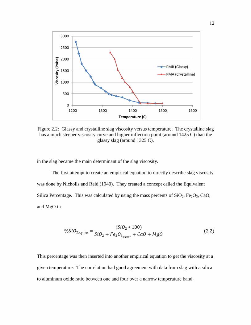
greatly increased as the liquid phase interacts with the newly formed solid phase. Figure
2.2 shows a plot of glassy and crystalline slag viscosities versus temperature.
Oh et al. (1995) theorize that this difference in behavior is due to the way the
mineral crystals in the slag form. Glassy slag tends to form long, linear crystals when
cooled. In contrast, the crystals formed in a crystalline slag tend to be dendritic, having
many branches. The branches of the crystals interact and bond with each other, causing
the slag to have greater viscosity and an increased melting point.
Cohen and Reid (1940) developed the Ferric Percentage, which they used as a
marker to identify crystalline slag, or slag of which the viscosity would increase greatly
with a small drop in temperature. The equation they empirically developed for this was
where all percentages are mass percents. They determined that any slag with a Ferric
Percentage over 20 would be very high viscosity (crystalline) and that the amount of iron
12
Figure 2.2: Glassy and crystalline slag viscosity versus temperature. The crystalline slag
has a much steeper viscosity curve and higher inflection point (around 1425 C) than the
glassy slag (around 1325 C).
in the slag became the main determinant of the slag viscosity.
The first attempt to create an empirical equation to directly describe slag viscosity
was done by Nicholls and Reid (1940). They created a concept called the Equivalent
Silica Percentage. This was calculated by using the mass percents of SiO2, Fe2O3, CaO,
and MgO in
This percentage was then inserted into another empirical equation to get the viscosity at a
given temperature. The correlation had good agreement with data from slag with a silica
to aluminum oxide ratio between one and four over a narrow temperature band.
0
500
1000
1500
2000
2500
3000
1200 1300 1400 1500 1600
Vis
cosi
ty (
Po
ise
)
Temperature (C)
PMB (Glassy)
PMA (Crystalline)
13
Later, the work of Cohen and Reid (1944) was used to create a prediction of the
thickness of the slag layer on a furnace surface. Later still, they worked to develop
empirical relations to describe the build-up of slag on tubes inside of a coal combustion
furnace (Reid and Cohen 1944a).
Cohen and Reid (1940) also developed a viscosity equation, basing it on a power
function. The equation they created to describe their observations was
(
)
where Z, and A were empirically derived constants, B is a composition-dependent
constant, ηis the viscosity in poise and T is temperature in Kelvin (Reid and Cohen
1944b).
Another noteworthy model of slag critical viscosity temperature was developed
by Sage and McIlroy (1959). They took the innovative approach to divide the minerals
present in slag into acidic or basic groups. The ratio of these two groups and the
temperature of the slag were then inserted into an empirical equation to predict the slag
viscosity. In this model, silicon, aluminum and titanium are considered acidic while iron,
calcium, magnesium, sodium and potassium are considered to be basic. The basic
minerals all only bond with 1 or ½ oxygen atoms (such as calcium or magnesium), which
would theoretically contribute to a weaker crystal matrix within the slag. The acidic
minerals each bond with 1 ½ or more oxygen atoms (such as iron, silicon, or titanium),
thereby creating a stronger matrix as more possibilities to bond will result in a more

14
networked arrangement of molecules. The ratio of the mass percent of acidic and basic
minerals (A/B) is inserted into,
(
)
to get the Tcv value. Streeter et al. (1984) examined the accuracy of this equation by
employing it on a large sample of low-rank coals. According to their work, after some
modifications of the constants, the equation gives good results for coals with iron content
of less than 10% by mass of the total mineral content and an acid/base ratio between one
and seven.
The next major milestone in the slag viscosity literature is the Watt and Fereday
(1969) model. They had the goal of creating a model that would be better suited to a
wide range of British coals. They were concerned that the previously developed models,
which used American coals as their basis, would not accurately describe the behavior of
wide-ranging British coals. The Watt-Fereday model focused on the effect of silica,
aluminum oxide, calcium oxide, iron oxide. They analyzed the viscosity curves of 113
different coals and used a regression fit to create an equation similar to the Arrhenius
equation in form:
where m and c are constants based on composition,

15
where all oxides are evaluated as mass percents and the iron equivalent was determined
as per eq 2.1.
The Watt-Fereday model was determined to be very useful over a wide range of
slag compositions. In previous models, calcium, magnesium, and iron were all
considered to have equal fluxing efficiency. Through their research they discovered that
not all fluxing minerals have an equal effect on the final slag viscosity.
In 1981, Urbain set out to further improve viscosity predictions by applying the
concepts of network formers and modifiers as found in glass formation theory. Urbain
considered the work of both Weymann (1962) and Frenkel (1955) who had both done
work on modeling silicate glass viscosities. The Weymann-Frenkel model for viscosity
was similar to the Watt-Fereday model in that it used an Arrhenius-type equation,
(
)
where T is temperature in Kelvin, η is the viscosity of the slag in units of poise and A and
B are constants that are dependent on the slag composition. Urbain (1981) postulated
that it should be possible to simplify the model by creating dependency between the A
and B constants. By studying 60 different silicate melts, they determined that the two
constants could be linked by

16
The group then determined B would be related to the mole fraction of silica in the melt,
as per
where N is the silica mole percent in the melt. The empirically determined values of the
Bi values were influenced by the ratio of calcium oxide to the total of calcium oxide and
aluminum(II) oxide, . For example, B0 was given by the parabolic equation
Three additional equations were given for the other Bi constants in the literature but are
not presented here.
Although the Urbain model was fairly successful at predicting slag viscosities, it
was really the simplicity and flexibility of the model that set it apart. The Urbain model
is important in that many modern models are variations or modifications of it.
Kalmanovitch and Frank (1990) tested several of the existing models and found
that the Urbain model was the most accurate. They also refined the Urbain equations and
expanded them to be able to consider slag containing iron, magnesium, sodium,
potassium and titanium, which had previously been neglected in calculations. They
modified the alpha value to be

17
rather than the simple ratio between calcium oxide and the sum of calcium oxide and
aluminum(II) oxide.
In another example of modifying the Urbain model, Senior and Srinivasachar
(1995) used the Urbain model and expanded it to apply to slag at much higher viscosities.
Previous models were only applicable to the relatively low viscosity range of 102-10
3
Pa·s, but the Senior-Srinivasachar model could be applied to the 104-10
8 Pa·s range. This
was important as it helped to make better predictions of slag behavior at lower
temperatures, before the Tcv of the slag had been reached. Much of the slag that sticks to
furnace pipes and surfaces is below the Tcv, so this model could be directly applied to
improve deposition models.
The basic form of the Senior-Srinivasachar model is an empirical equation of the
form
(
)
where A and B are composition and temperature dependent variables. Each The B
variable is a function of N, the mole fraction of SiO2 in the slag, and which is defined
as
18
where xi is the mole fraction of the indicated mineral.
In order to add validity to their model at lower temperatures, Senior and
Srinivasachar divided the viscosity-temperature into two parts at the Tcv point. The A and
B variables each have two values, one for use at temperatures above the Tcv and the other
for lower temperatures.
The equation for the B value was set determined to be
where each bi is a curve fit parameter. The final value for these constants is given in
Table 2.2. The high and low-temperature B values were calculated to be 12.03 and 77.66
respectively.
The A value is dependent on the B value and the ratio of non-binding oxygen to
tetrahedral oxygen (NBO/T),
The NBO/T value for the coal used was calculated to be 0.87. The equation for A in the
high temperature region was determined to be

19
Table 2.2. Fitted values for bi
Constant High Temperature Low Temperature
b1 -224.98 -7563.46
b2 636.67 24431.69
b3 -418.70 32644.26
b4 823.89 -103681.0
b5 -2398.32 74541.33
b6 1650.56 -46484.8
b7 -957.94 146008.4
b8 3366.61 -104306.0
b9 -2551.71 21904.63
b10 -1722.24 -68194.8
b11 1432.08 48429.31
and the low-temperature equation for the related NBO/T value was
The high and low-temperature A values were determined to be -8.70 and -69.94
respectively.

20
The Browning (BBHLW) model has taken a different approach to predicting slag
viscosity. Browning et al. (2003) started with the assumption that at a given viscosity,
the gradient of a slag temperature/viscosity curve is equal to any other at that same
viscosity and that therefore all slag viscosity curves could be normalized to fit a standard
curve. This is based on the observation of Nicholls and Reid (1940) that the change in
viscosity with respect to temperature is related to the viscosity and not the temperature, or
in equation form,
To normalize the slag viscosity curves, they relate the viscosity to a modified temperature
by subtracting from the measured temperature a temperature shift, labeled TS. The TS
term is calculated from
The TS value is dependent on composition, as the A term is calculated from
The resulting equation is
21
(
)
The results of this unique approach had better accuracy than the Kalmanovitch/Urbain
model, particularly for natural slag, but it was still limited to temperatures and viscosities
above the Tcv of the slag.
Another idea to improve model predictions was first proposed by Van Dyk et al.
(2009). They postulated that a way to improve the model accuracy would be to take into
account the formation of solids inside the slag as the formation of these solid crystals
would result in a small change in the composition of the liquid phase. Van Dyk et al.
employed the FactSageTM
thermochemical database software package to determine any
solidification. The composition of the predicted liquid phase was plugged into the KF
model, developed by Kalmanovitch and Frank (1990). The results were an improvement
in accuracy over the base model without using FactSageTM
.
Kondratiev and Jak (2001) also attempted to improve on other models by taking
the solid phase into account. They postulated that as a slag crystallized, certain minerals
were more likely to precipitate than others. Thus the remaining liquid slag may have a
different composition than the overall slag composition. As Van Dyk et al. did,
Kondratiev and Jak used the F*A*C*T* software program (later integrated into the
FactSage software) to predict the leftover liquid composition in the slag after
crystallization had been taken into account. For the viscosity predictions they employed
a modified version of the Urbain equation. The α term was modified to include all
modifiers and amphoterics as per

22
where the X terms represent the mole fractions of modifier or amphoterics in the slag.
They developed a global B term to describe the interactions of all the modifiers and
amphoterics at once,
∑
∑∑(
) (
)
where XA, XC, XF, and XS represent the mole fractions of aluminum(II) oxide, calcium
oxide, iron(II) oxide and silica. The b terms are empirical parameters that were used to
fit the model to experimental data. By combining the modified Urbain model with the
use of F*A*C*T* they were able greatly increase the accuracy of viscosity predictions
over those of the original Urbain model.
More recently, as computational power has expanded, attempts have been made to
use artificial neural network models to describe the slag viscosity behavior, such as the
one developed by Folkedahl (1997). Artificial neural networks are designed to act
similarly to an organic brain. The network model has various input nodes that feed the
data to a set of “hidden” nodes. The hidden nodes then interact to produce the output
value, similar to neurons interacting to remember or interpret information. The input
nodes in a slag viscosity model would be the temperature and composition and the output
would be the fluid viscosity. Neural networks are more flexible than a purely empirical
relation, but may be less accurate and must be trained with large volumes of information.

23
For example, Folkedahl used a data set of 18,000 points of slag composition,
temperature, and viscosity data. The neural network he created gave results that better
matched the experimental results than those predicted by the Urbain or Senior-
Srinivasachar models over certain temperature ranges.
Duchesne et al. (2010) also developed an artificial neural network model. Their
model was created solely to predict the viscosity of Genesee coal, but over a wide range
of temperatures. They compared the results of the neural network model with several
other empirical correlations including the Watt-Fereday, Urbain, and S2 models. The
neural network model outperformed all of the empirically derived models by a very
significant margin. In some cases the empirical models mis-predicted by orders of
magnitude, while the neural network model only had an absolute error of 5.
Each model presented above has strengths and weaknesses and no model can be
easily applied to all cases. Artificial neural network modeling is very interesting and can
achieve very good results; however the amount of data and time required for training the
model will be prohibitive to its wide use. For most cases, a modified Urbain or
Weymann model will be sufficiently accurate.
2.3 Other Slag Property Studies
Although the viscosity-temperature behavior of slag has been focused on the most
by the research community, additional studies have been done to determine other
properties of slag and silicate melts. As preliminary research into using slag as a building
material, much as fly ash is used as an additive for concrete, Aineto et al. (2006) worked
to determine the thermal expansion of coal slag. They found that slag has a relatively
high thermal expansion compared to fly ash of the same particle diameter and determined
24
that this was due to the expansion and devolution of the trapped gasses inside the cooled
slag particles.
Bottinga and Weill (1970) studied the density of magmatic liquids. Assuming
silicate slag to be an ideal solution, they found that using a simple summation of partial
molar volumes of the minerals in the liquid yielded results as good as physical
measurements with an average error of less than 8%. Their equation was
∑
where Xi is the mole fraction of component i, Mi is the molecular weight of component i,
and is the partial molar volume of component i. This work has been successfully
applied to coal slag.
Additional work identifying slag properties was done by Mills and Rhine (1989).
Earlier, Grau and Masson (1976) theorized that in order to accurately calculate the
density of a silicate melt, the intermolecular forces needed to be considered. However
the model that they produced was not as successful at predicting density as the ideal
solution model of Bottinga and Weill. Mills and Rhine (1989) built up the work done by
Bottinga and Weill by taking into account the molecular interactions between different
mineral oxides. This resulted in an empirical equation with adjustments made to the
molar volumes of silica and aluminum oxide, which provided more accurate estimates of
the melt density.
Mills and Keene (1987) also developed a simple equation for the density of slag,

25
which was found to be accurate within 5%, despite its simplicity.
Mills (1986) also provided augmentations to equations to calculate the surface
tension and thermal expansion coefficients of slag. Up to that time, most equations to
predict the surface tension of silicate melts were based on a simple summation of the
contribution of the components, similar to eq 3.19,
∑
where i is the surface tension of component i (Boni and Derge, 1956; Popel, 1962).
Based on Mills’ own previous work, the slag components were divided into surface
active and surface inactive groups. The contribution of surface active components to the
slag surface tension was taken into account with a set of parabolic equations that were
inserted into the empirical equation. For example, the mole fraction of iron(II) oxide was
adjusted as per
Corrections were also offered for the oxides of sodium, potassium, phosphorous,
chromium, and sulfur. This new, adjusted equation successfully resulted in more realistic
results for surface tension calculations.

26
Methods of calculating heat capacity in slag have also been developed.
According to Mills et al. (2002), the Kopp-Neumann Law gives an accurate estimation of
the heat capacity of slag. This law states the heat capacity of a mixture is equal to the
sum of the product of the mass fraction of each component multiplied by the heat
capacity of the pure component,
∑
where Cp,i is the heat capacity of component i. Gohil and Mills (1981) developed an
empirical model to improve the accuracy of the results, but found little improvement over
the simple Kopp-Neumann Law.
Also found in the work of Mills and Rhine (1989) is an equation to describe the
effective thermal conductivity of slag,
where is the effective thermal conductivity, and aeff is the effective thermal
diffusivity. Many viscosity tests for slag employ a crucible and spindle viscometer. By
measuring the inner and outer temperatures, Mills and Rhine were able to determine the
thermal diffusivity, which they found to be 4.5x10⁻⁷
m2/s. Zbogar et al. (2005) state that
the conductivity should fall in the range of 0.6 ± 0.2 W/m K.
Finally, Mills and Rhine also determined the slag emissivity was equal to
They found the value to be independent of slag composition and determined

27
that it was constant for any temperature between 1070 K and 1800 K. Other work, such
as that performed by Bohnes et al. (2005), found a strong composition and temperature
dependence for the emissivity. Calcium, in particular, greatly increased the emissivity of
the slag.
2.4 Computational Modeling of Slag in a Reactor
Many groups have attempted to apply the previously discussed property models to
reactor simulations. The goal of these simulations is to accurately predict slag build-up,
general distribution, temperatures, and viscosity in order to minimize problems during
reactor operation. For example, in operating gasifiers, slag must be removed from the
reactor through a slag tap. In order to flow from the tap, the slag must be at a viscosity of
25 Pa·s or lower, otherwise the slag will fail to flow quickly enough and may plug the
gasifier (Song et al. 2009). Such an occurrence would mean having to shut down the
gasifier to remedy the problem.
There have been several groups that have successfully created computational
models of slag flow inside of a gasifier and their models will be discussed here. For each
model, a general overview is given and then some attention is paid to the details of what
viscosity model was used, how the Tcv was predicted and how in depth the treatment of
energy transfer was.
Seggiani (1998) created a model for a Prenflo gasifier to study what effect the
addition of fluxing agents would have on the slag thickness. A Prenflow gasifier differs
from an entrained-flow gasifier in that it is upward fired. Slag collects on the walls and
flows downwards toward a slag tap where it is collected. In order to keep the slag at a
viscosity low enough to be tapped, it is common to add limestone to act as a fluxant.
28
Seggiani’s model solved the Navier-Stokes equations in three dimensions using
the finite volumes method. To do this, he divided the gasifier into 15 volumes of
different heights, with smaller volumes filling the top and bottom of the gasifier for
increased accuracy in those zones.
To predict the slag Tcv values, Seggiani used the model created by Sage and
McIlroy, given previously in eq 3.6. For the temperature/viscosity relation, Seggiani
chose to use the BCURA S2 model, discussed in a previous section and summarized in
eqs 3.14 and 3.15. He states that the slag density and specific heat was calculated based
on the work of Bottinga and Weill (see eq 2.1). These were then used to calculate the
thermal conductivity, based on a thermal diffusivity of α = 4.5 x 10⁻⁷
m2 s
-1, as reported
by Mills & Rhine (1989). The emissivity of the slag was set to 0.83, also based on the
work of Mills and Rhine.
Seggiani included an ash deposition and slag build-up model. Apart from the
needed mass and momentum balances, Seggiani’s model also included an energy
balance. This included radiation to and from the slag and included heat loss through
refractory via conduction.
Seggiani’s model was important for many reasons. First, it was the first full
simulation performed for slag flow in a gasifier, and it was very successful at predicting
slag levels inside the gasifier with varying amount of added fluxant. Second, even
though it was the first model of its kind, it was a complete three-dimensional model.
Third, it was brought several other empirical models together and demonstrated that it
was possible to couple these equations into a full reactor simulation. Seggiani’s work
continues to be studied and replicated even today and has been cited over 250 times.

29
Bockelie et al. (2001) modeled the slag flow in a downward-fired, entrained-
flow gasifier as a submodel for a larger simulation. The larger simulation included fluid
dynamics for the reactor, char gasification and devolatilization, and ash deposition on the
reactor walls.
For the slag flow submodel, the reactor walls were divided into two-dimensional
vertical strips. For each strip, first a heat transfer calculation was made to determine the
temperature distribution through the slag layer. From this, thickness at which the slag
was at its Tcv was determined. Any slag cooler than the Tcv was assumed to be solid and
immobile while the liquid slag was assumed to be at a uniform average temperature. The
two-dimensional Navier-Stokes equation was solved for the liquid slag for each strip
simultaneously. Fluid was allowed to move between the strips, however, as the reactor
walls were clear of any impediments the fluid simply flowed downward to a great degree.
These results for each strip were then patched together into a pseudo-three-dimensional
result. The model was able to qualitatively predict slag thickness and to point to sections
in the gasifier where the slag was prone to build up.
The model by Bockelie et al. included an energy balance that accounted for heat
loss through the refractory and allowed the slag to freeze into a solid mass. All heat
transfer to the slag layers was assumed to only come from heat radiated from the flame.
Convective heat from the hot gases inside the reactor was ignored, as were the convective
losses from the slag flowing over the refractory or frozen slag. Temperature across the
slag layer was calculated as a gradient.
Bockelie et al. used the model developed by Patterson et al. (2001) to calculate
the Tcv and viscosity of the slag. The Patterson model was developed to predict the

30
viscosity behavior of Australian coals, but was applied here due to similar ash
composition. No information was given on how the density, specific heat, or thermal
conductivity of the slag was calculated.
Ni et al. (2010) created a model of a slagging gasifier. This model was significant
for two reasons. First, they removed the assumption of an average temperature
distribution in the slag layer, which had been used in many of the previous models.
Second, they considered the convective heat transfer of the reaction gases to the slag. It
is also noteworthy that the model was developed in the Ansys Fluent program.
Ni et al. modeled both refractory-lined and actively cooled gasifiers. As with
other models, slag below the Tcv was considered to be solid. Liquid slag temperature was
not averaged over the entire layer, but was instead calculated for each cell. Temperature
dependent properties were also calculated in this manner.
The team used the Weymann viscosity model for their slag as it fit the
compositions of the coals they were testing. Comparison of the slag deposition thickness
as predicted by their model results to the results of real experiments showed very good
agreement.
2.5 Jet Impinging on Thin Film Studies
One component of the research performed in this study concerns the penetration
of a gas jet through a falling viscous liquid film. Efforts were made to identify literature
related to such studies. However, it appears that no studies on this phenomenon have
ever been reported. There is a large amount of literature dedicated to the study of gas jets
in cross flow (JICF); the phenomenon has been studied in great detail, but the work is

31
concerned with the behavior of the jet as it penetrates the fluid where the present research
is concerned with the behavior of the fluid as it is penetrated by the gas jet.
Banks and Chandrasekhara (1963) performed a study on surface deformation of a
fluid when impacted by a gas jet. They found that the size of the cavity a jet would cause
to form in a fluid surface is related to the fluid density and surface tension and the jet
geometry and velocity.
The concept of a Weber number is very prominent in the area of jet and fluid
behaviors. The Weber number is the ratio of the kinetic energy of a droplet and its
surface energy. Weber numbers are often used to quantify the behavior of falling
droplets upon impact with a surface.
The Weber number has been modified to be applicable to a droplet being struck
by a jet stream. Tambe (2004) and Joseph et al. (1999) used such a modified Weber
number to determine the conditions at which droplets would be broken up when exposed
to a cross jet.
Senecal (1999) and Nagabhushana Rao and Ramamurthi (2010) also modified the
Weber number to apply the breakup of liquid sheets. They studied liquid sheets being
broken up by parallel flowing gas jets. They found that to produce a particular droplet
size, the gas jet velocity had to be adjusted so that the resulting Weber number was equal
to 27/16.
2.6 Summary
For the current study, the information regarding coal slag properties is very
important. Particularly, the viscosity models were very carefully considered. Due to the
ability of the Senior-Srinivasachar model to predict slag viscosities below the TCV, this

32
model was applied to the computational models. The empirical correlations for other slag
properties such as density and heat capacity are also very important to this work and
several of them were used to estimate the slag properties for the model.
The concept of a Weber number, while not directly applicable to this work, did
greatly influence the dimensional analysis of the physical model. The work done by
previous authors on the Weber number also helped to clarify which variables would be
the most important to consider in the physical model.
CHAPTER 3
OBJECTIVE AND APPROACH
3.1 Objective
Three major objectives were identified for this work. The first objective was to
study the behavior of a viscous film and an impinging jet. It was desired to understand
how a viscous film, such as the slag film present in a coal gasifier, would respond to an
impinging jet. It was anticipated that the results of these studies could be reduced to a
single parameter to describe the system, as a Reynolds number does for fluid flow or a
Weber number does for a falling droplet.
The second was to develop physical and computational models to describe the
slag behavior so that different methods of slag diversion could be tested. The models
should serve to isolate the most important properties of the slag flow, such as the variable
viscosity, so that each property can be studied independently.
The final objective was to use the insight gained from the completion of the first
two objectives to develop a reliable method for maintaining a clear line of sight across a
real reactor. The diversion method should create a completely clear line of sight for
many hours at a time in order to be considered successful. Interference with normal
operation of the gasifier should be minimized.

34
3.2 Proposed Methods
Two different methods of diverting the slag were considered: A purge gas jet and
a solid tube to interrupt the slag film and divert it around the sight port. The purge gas jet
method will be discussed first.
The first method, called the jet diversion method, involves employing a purge gas
jet set inside the reactor-side face of the sight port and aimed upward to impact the slag
as it arrives at the top of the sight port opening. It was theorized that the momentum of
the jet would stop the slag flow and force it to flow around the hole instead. A diagram is
shown in Figure 3.1 to illustrate the idea.
This method has several points in its favor, such as high adjustability. As the slag
rate changes, the flow rate of the jet can be adjusted to compensate. Also, it is projected
that the purge flow would keep the device relatively cool, allowing it to be a permanent
fixture in the gasifier.
There were also disadvantages to the jet diversion method. The geometry of the
gasifier would make precisely aiming the device difficult. Also, using a high flow rate of
purge would dilute the gasifier reaction and lower performance. Lower temperatures
would result in higher slag viscosity, which could cause serious complications such as
gasifier plugging.
The second method studied, called the tube diversion method, consists of creating
a physical diversion of refractory material or alumina set above the sight port. A search of
the literature revealed that slag can wear refractory at very high rates. According to
Bakker (1984), this may exceed 0.20 mm/hr under extreme conditions. Creating a
diverter of refractory that would protrude into the reaction section of the reactor enough

35
Figure 3.1. Diagram of the gas jet diversion method. The slag flows down the wall from
above and, as it reaches the opening in the wall, is struck by a gas jet. The momentum of
the jet causes the slag to move to the side. This keeps the sight port clear for optical
access.
to impact the slag flow patterns would leave it exposed to additional erosive forces of the
reactant stream and the thermal stress from the flame. There was great concern that such
a structure would not last long in a reactor due to the erosive force of the slag flow and
the chemical attack such a device would endure from the slag. As an alternative, a
hollow alumina tube was chosen to be inserted a short distance into the reaction section.
The tube would pierce the slag film and provide a line of sight into the reactor.

36
The tube diversion method presented advantages in that it would be simpler to
implement than the jet diversion method and it would have a reduced purge gas usage,
which would interfere less with gasifier performance. However, a lack of adjustability
during gasifier operation is a potential drawback.
3.3 Approach
Performing experiments with real slag samples would be prohibitively expensive.
Slag has a very high melting point, 1500 K or above depending on the mineral
composition. It also hardens quickly when cooled, making it difficult to work with. To
avoid the costs and dangers inherent in live slag experiments, it was proposed to use a
simplified physical model and a computational model to study the feasibility of the two
proposed diversion methods before implementing them into the gasifier.
A physical model using viscous silicone oil as the slag was proposed to study the
impacts of film viscosity, surface tension, and flow rate. Specifically for the jet diversion
method, the jet flow rate and impingement angle would also be studied. The flow rates at
which a clear line of sight was established for these variables would be recorded and
analyzed. For the hollow tube method, the approximate length of tube required to
maintain the line of sight would be recorded.
To study the interaction of fluid flow and the heat transfer effects, particularly the
heat transfer between the slag and the jet, a computational model was proposed. The
computational model would use the Fluent software package to model a small part of the
interior of the gasifier and be applied to each proposed method. The possibility of slag
cooling and freezing would be studied. The model would be validated by comparing

37
computational results without heat transfer to those of the physical, silicone oil-based
results.
It was predicted that by combining the results of the physical and computational
models, an efficient and effective method of creating slag diversion around the sight ports
in the reactor could be found. It was also expected that an empirical correlation could be
developed that will predict the fluid diversion behavior for a particular system whose
inputs, such as fluid velocity, viscosity and purge jet mass flow rate, are known.
It was proposed to fabricate devices and apply each of them to the entrained-flow
gasifier available at the University of Utah facilities for live tests.

CHAPTER 4
EXPERIMENTAL
4.1 Introduction
To gain a better understanding of the physics involved in altering the slag flow,
several experimental approaches were made. A physical model was used to act as a proof
of concept for each diversion method. Computational models were also used to examine
how heat transfer effects could affect the diversion devices. The computational model
also provided a convenient way to optimize the operating conditions of each method.
Finally, each method was tested in a pilot-scale gasifier. In this chapter the models and
devices created are detailed.
4.2 Silicone Oil Model
4.2.1 Apparatus
The silicone oil experiments were devised as an inexpensive and safe way to test
the two slag diversion methods. Using silicone oil as a substitute for slag allowed careful
examination of the physics involved with both diversion methods without risk of
handling very high temperature material. With these physical models, the effects of film
mass flow rate, viscosity, and the jet flow rate and impingement angle could be
considered and precisely measured.

39
Tests were performed for both the jet and the tube diversion methods. A unique
experimental apparatus was created for each. For each of the setups, the scale of the
geometry was set to be true to that of the actual reactor. However, the physical model for
the jet method experiments was performed using a flat wall rather than a curved one.
The experimental setup for the jet method tests, as shown in Figures 4.1 and 4.2,
consisted of a vertical wall for the liquid film to flow down, a liquid recirculation system,
and a gas jet control system. The vertical wall was made of a 55 x 37.5 cm smooth
surface board. An elliptical hole measuring 3.5 x 20 cm was cut out of the wall for the jet
to pass through. The hole is centered in the board, and the top of the hole is located
approximately 22 cm down from the top of the wall. The wall was suspended on a
support structure over the liquid reservoir so that the fluid falling from the wall would be
captured and reused.
A variable-speed, two stage, positive-displacement pump (Moyno Industrial
Products, Model 34408, 2.8 lpm max flow rate) capable of pumping high-viscosity fluids
circulated the liquid from the reservoir to a distributor at the top of the wall. The pump
was powered by a three-phase electric motor (Baldor Electric Company, Model M3538,
370 W max output).
The liquid distributor is made from a 1 cm OD tube attached horizontally to the
top of the wall with 2 mm holes drilled at a regular spacing. To get an even film
distribution, the spacing is set so that more holes exist near the center of the tube. The
liquid flow is directed downward against the board at a 30 degree angle, thus creating a
thin film that flows down under the influence of gravity. The film flows down the wall

40
Figure 4.1. Schematic of physical model setup. The hatched area represents the wall for
the film formation. The nozzle of the gas jet was attached to a leveled protractor so that
the angle could be easily adjusted.

41
Figure 4.2. Geometry of the wall for the oil tests. All units are in mm. The elliptical slot
is shown in the wall and within the slot the tube and protractor can be seen.
surface, and across the elliptical hole, creating a suspended film for the impinging jet.
The film drips off the bottom of the wall into the reservoir.
The gas jet nozzle is a simple capillary made of a 4.6 mm ID (5.5 mm OD) steel
tube. It is situated inside the elliptical slot in the wall and recessed 13mm from the liquid
film surface as shown in Figures 4.3 and 4.4. The back of the hole was left open to allow
the gas to escape after impacting the film.
42
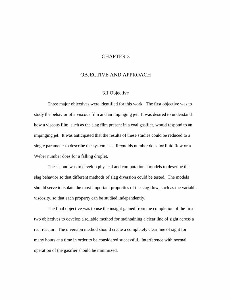
Figure 4.3. Jet impingement angle measurement.
The tube is attached to a leveled protractor so that the angle of the jet can be
measured and freely adjusted from 0 to 60 degrees. A zero degrees angle of impingement
corresponds to the jet being set perpendicular to the flow of the oil film, as illustrated in
Figure 4.3.
The gas jet flow rate is measured using a pair of high-precision rotameters
calibrated to measure gas flow rates from 0-50 SCFH and 0-200 SCFH (0-24 and 0-94
SLPM) (Dwyer Instruments, Michigan City, IN). The measured volumetric flow rates
were converted to mass flow rates using the ideal gas law. For the experiments presented
here, dry, filtered compressed air was used for the gas jet.

43
Figure 4.4. Tube within the elliptical slot. The tube was recessed 13 mm from the board
face when the angle was set to zero degrees.

44
The jet flow rate ranged from 10.0 SCFH (4.7 SLPM) to 36.0 SCFH (17.0
SLPM). Assuming the ideal gas law, this is equivalent to 0.096 g/s to 0.35 g/s. The
Reynolds number was calculated for these flow rates using
where Q is the volumetric flow rate in m3/s, r is the radius in m, and v is the kinematic
viscosity of the air in m2/s (de Nevers 2005). The Reynolds number ranged from 140 to
500 and so the flow was assumed to be laminar for all conditions.
The second apparatus used for the tube method experiments was very similar to
the first and followed the schematic shown in Figure 4.1. However, for these tests, the
curved geometry of the gasifier was included in the design, as it was theorized that in
such a scenario that the curved surface would have more influence than in the jet method.
To create the curved surface the flat board was replaced with a cast piece of refractory.
The piece was cast to have the same curvature and to have a sight hole the same size as
that of the University of Utah’s coal gasifier. The dimensions of the unit are shown in
Figure 4.5.
A fluid distributor was made for the refractory wall. It is made of 1.25 cm OD
(1.1 cm ID) steel tubing and has been bent to fit the curvature of the cast. The distributor
is butted up against the top of the refractory and held in place with clamps. The tube has
2 mm holes drilled at regular intervals for the silicone oil to pass through. The holes are
arranged so that a greater concentration of holes is at the center of the tube. This was
done to achieve an even distribution of silicone oil across the refractory face. To promote
film formation, the holes are angled downward about 30o when the distributor is attached.
45
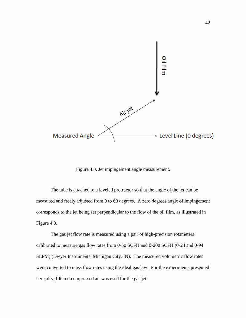
Figure 4.5. Dimensions of the refractory cast. The cast represented here was used for the
hollow tube experiments. All units are in cm. Curvature of the refractory was set to
match that of the inner refractory layer of the pilot-scale gasifier.
This prevents the oil from accumulating in the small gap between the tube and the
refractory and spilling into unwanted places.
4.2.2 Samples
Silicone oil (Clearco, Bensalem, PA) was chosen for these experiments because
its properties are well known and documented and it is available in a wide range of
viscosities. It was theorized that the viscosity of the film would be significantly affect the
behavior of the film when struck with the impinging jet. For this reason, it was important

46
to have films of variable viscosity without greatly changing the other parameters, such as
density or surface tension.
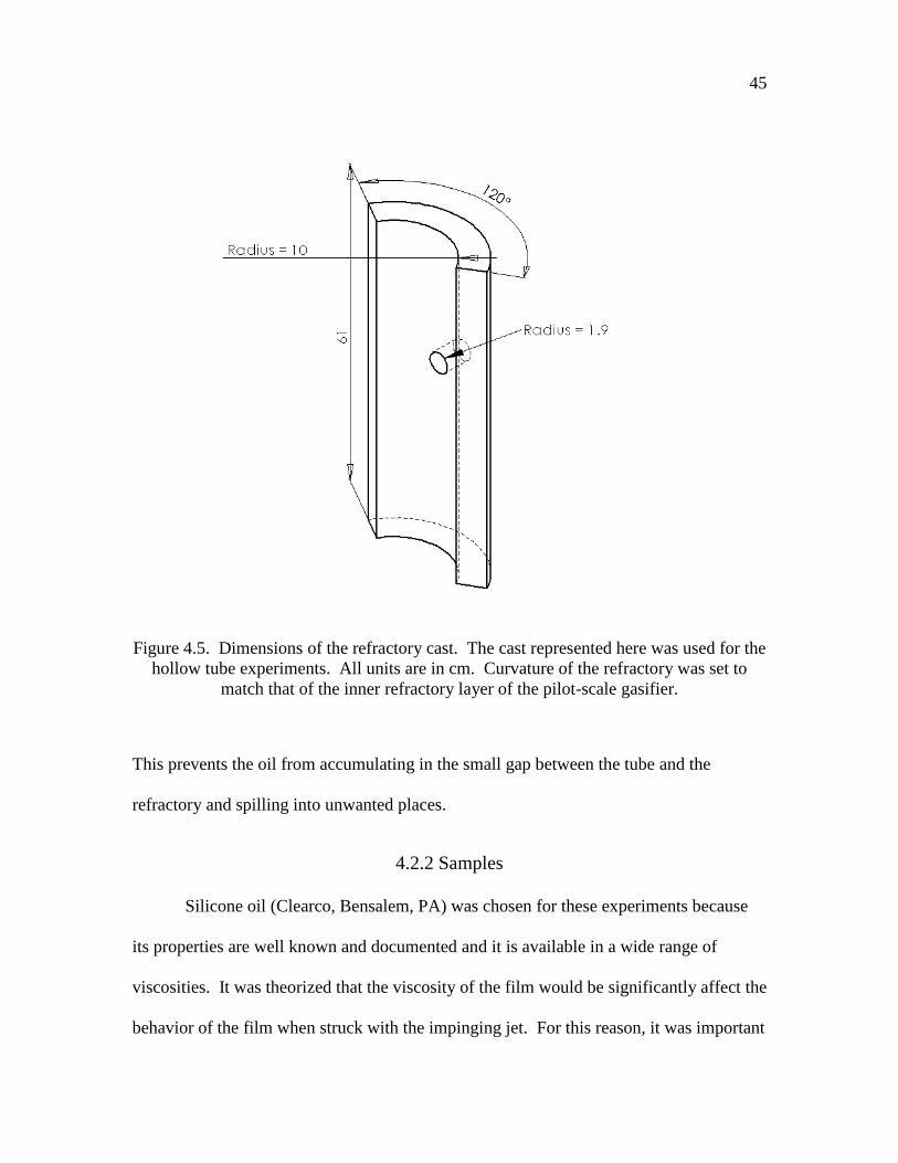
Silicone oil is made of polymerized dimethylsiloxanes, structure shown in Figure
4.6. The viscosity of the oil can be controlled by altering the length of the polymers in
the oil. Longer, higher molecular weight polymer chains make a more viscous fluid than
shorter chains (Friedman 1975). By controlling the average molecular weight of the
chains, a broad range of viscosities of oil can be made. Oils with viscosities of 30,000
cSt, 12,500 cSt, 5,000 cSt, and 100 cSt were used.
The density of each sample was calculated using a 50 mL volumetric flask and a
balance. For each calculation, the mass of the clean volumetric flask was measured on
the balance. The flask was then filled with 50 mL of an oil sample and again the mass
was measured. The original mass of the flask was subtracted from the result and then
divided by the 50 mL volume to obtain the sample density. This was repeated three times
for each sample. As expected, the density of the samples had little variance and averaged
976 kg/m3.
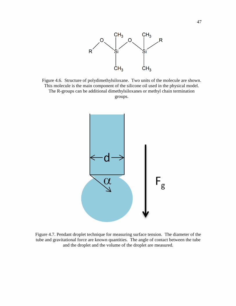
The surface tension of each sample was also measured using a pendant drop
technique. A fellow student, Vasiliy Chernyshev constructed the machine used to
conduct the surface tension measurements. Details of this measurement method are
given in Appendix D and an illustration of the technique is shown in Figure 4.7.
The properties of each sample are summarized in Table 4.1. The surface tension
averaged 21.1 mN/m and did not show much variation. This value is in line with other
values reported in the literature (Schurch et al. 1976; Carré and Woehl 2006).
47
Figure 4.6. Structure of polydimethylsiloxane. Two units of the molecule are shown.
This molecule is the main component of the silicone oil used in the physical model.
The R-groups can be additional dimethylsiloxanes or methyl chain termination
groups.
Figure 4.7. Pendant droplet technique for measuring surface tension. The diameter of the
tube and gravitational force are known quantities. The angle of contact between the tube
and the droplet and the volume of the droplet are measured.

48
Table 4.1, Silicone oil sample properties. Table includes values for the kinematic
viscosity, density, and surface tension.
Sample Kinematic Viscosity (cSt) Density (kg/m3) Surface Tension (mN/m)
1 100 975 21.3
2 5000 978 21.0
3 125000 976 21.4
4 30000 975 20.8
4.2.3 Procedure
4.2.3.1 Impinging Jet Tests
Prior to each series of measurements, the liquid circulation system was cleaned
and the silicone oil with the desired viscosity was loaded into the pump and reservoir
system. The pump was primed and the system was run to remove any residual air
bubbles from the oil lines. The angle of the impinging gas jet was adjusted and
confirmed using the attached protractor. The distance between the jet tip and outer wall
surface was confirmed to be 13 mm.
For each experiment, the pump was turned on and the liquid was allowed to flow
down the board until a uniform film flow had been established. The liquid flow rate was
varied between 0.03 and 0.10 l/min by adjusting the speed of the pump motor in order to
produce the desired film mass flow rate or thickness. For example, a majority of the
experiments were performed with a film thickness 5.0 mm, which corresponded to a
liquid film flow rate of 0.25 g/cm-s. Less viscous oils required higher mass flow rates to
achieve the desired film thickness.

49
After any adjustment of the pump speed, the mass flow rate of the oil was
confirmed, and thereby the thickness of the film was also confirmed. As the oil fell off
the board into the reservoir, it would accumulate into a single falling stream. This stream
was collected in a clean beaker, the mass of which had been previously measured. The
time of collection was measured with a stopwatch so that the mass flow rate could be
calculated.
For the purge jet experiments, once the desired oil film flow had been achieved
and the flow appeared to be stable, the air jet was slowly opened, at an approximate rate
of +0.25 SLPM/sec as the behavior of the two fluids was observed. The jet flow rate was
increased until the oil film burst open and the film began to divert around the jet flow.
Once the liquid film burst open, the corresponding jet flow rate was noted. The air was
then shut off and the oil film was allowed to return to a uniform flow.
The experiment was repeated several times, except that in the subsequent tests,
extra care was taken near the previously recorded bursting flow rate. The flow rate of the
jet was increased very slowly so as to get a precise measure of the jet flow rate when film
bursting occurred. Approximately 5 seconds time was given between each increase in the
jet flow rate.
After finding the gas jet flow rate required to burst the oil film, a similar process
was used to determine the flow at which the oil film would flow over the jet flow path
and reform a closed film. The gas jet flow rate was first adjusted to twice that which had
been required to burst the film, and was slowly reduced at -0.25 SLPM/sec until the
opening in the oil film closed. Again, once the flow rate was determined, experiments
were repeated with more careful decreases in the gas flow rate. The system was allowed

50
to operate for several seconds between adjustments until the precise flow rate at which
film diversion closure occurred had been precisely determined.
The impingement angles tested varied across the different oil viscosities. Each of
the four oils was tested at 0o, 10
o, 15
o, 30
o, 45
o, 50
o, and 60
o angles. Some oils were
tested at intermediate angles when more data points were desired.
4.2.3.2 Tube Diversion Tests
The objective of the performing the tube diversion method tests was to gain a
qualitative understanding of how the fluid film would behave upon impacting the tube.
Thus the tube tests were done in a less precise manner.
Before each set of experiments, the pump and associated tubing were cleared of
residual oil and the desired viscosity oil was loaded into the pump fluid reservoir. A
hollow alumina or PVC tube was placed in the sight port of the refractory cast so that a 4
cm length protruded from the inner curved surface of the refractory into the path of the
oil film. The tubes had an outer diameter of 3.2 cm.
The pump was then initiated and the rate was adjusted to produce a film of the
desired thickness. After any pump speed adjustment, the oil film mass flow rate was
confirmed as described previously in this section.
The behavior of the film as it met the tube was observed. At the impact area, the
oil accumulated and formed a lip on the tube, as shown in Figure 4.8. Once this lip had
stabilized, the thickness of the lip from the refractory face was measured.
After measuring the silicone oil lip on the alumina tube, the tube was slowly, in
0.25 cm increments, pulled back out of the refractory, reducing the exposed section.

51
Figure 4.8. Silicone oil on impact with the tube. As the oil impacted on the tube, a lip
formed on top of the protrusion. The thickness of this lip was measured from the
refractory face.
After each adjustment, the flow was allowed to stabilize. This was continued until the oil
overran the lip of the alumina tube and spilled over into the line of sight.
These tests were repeated for three oil film mass flow rates. The first flow rate
was based on an estimation of the slag flow rate on the walls of the gasifier. The second
and third flow rates were set to be double and quadruple of the first to test the robustness
of the design of the tube diversion method.
52
It should be noted that the thickness of the produced film was not directly
measured in any of the experiments because insertion of any measurement device would
disturb the oil flow. Instead the film thickness was calculated based on the measured film
mass flow rate. From the work of Bird et al. (2002) the thickness of a falling film such
the one presented here is
√
where is the thickness of the film in m, is the kinematic viscosity, is the mass flow
rate of the film in kg/s, W is the width of the film flow in m, and is the angle between
the direction of flow and gravity (zero in this case, thus cos(0) = 1). The method
executed to arrive at this equation is presented in Appendix A.
Such an equation depends on the assumption that the fluid is Newtonian.
Although silicone oil is non-Newtonian, studies of the material by Carré & Woehl (2006)
determined that it behaves as a Newtonian fluid until shear rate exceeds a critical value,
in this case approximately 1000 s-1
. During such shear, the fluid becomes shear-thinning,
exhibiting less viscosity as increasing shear rate is applied.
In the system under consideration here, the shear rate on the fluid was not
measured. However, Appendix B shows a quick exercise to prove that the fluid stayed
well within the Newtonian regime.

53
4.3 Computational Model
The physical silicone oil models provided good information about the feasibility
of the proposed diversion methods. They also helped to determine optimal operating
conditions for both of the diversion methods. However, the physical models were not
able to predict the effects of heat transfer on the slag behavior.
In particular, the tendency of the slag viscosity to greatly increase with decreasing
temperatures was of great concern. Several questions were raised:
- As the impinging jet cooled the slag, would the heat transfer from the
reaction gases and flame be sufficient to maintain the slag in a liquidus state
or would the slag freeze into a solid block?
- If the slag froze, would it maintain a constant position or continue to slowly
flow?
- Would any solid slag help or hinder the diversion of the slag film?
These questions could not be answered using the silicone oil model. Thus the
computational models were developed to take the heat transfer effects of the system into
account.
Two separate geometries were created to mimic the apparatus used for each of the
silicone oil tests. This was done so that the results of the silicone oil tests could serve as
validation of the computational model.

54
4.3.1 Geometry and Boundary Conditions
4.3.1.1 Jet Diversion Model
The geometry for the jet diversion method computational model is shown in
Figure 4.9. It consists of a flat, vertical plane measuring 200 x 385 mm. A cylindrical,
22 mm diameter hole is set centered horizontally in the board, 181 mm from the top.
Within the hole, a 5.5 mm OD (4.4 mm ID) tube is set at a 45 degree angle so that the
tube is aimed at the point where the topmost part of the cylinder intersects with the
vertical plane. The tube is recessed 13 mm from the vertical plane surface.
All of the wall which the film traverses was a no-slip wall boundary. . In order to
reduce demand for computation time, the geometry was split in half with a plane that sits
perpendicular to the vertical wall. This new plane was assumed to be a symmetry
boundary for the experiments.
Also in Figure 4.9, the jet inlet boundary can be seen. This is shown in greater
detail in Figure 4.10. The semicircle at the bottom of the jet was appointed as a mass
flow inlet boundary for the jet. This allowed the flow rate of the jet to be easily adjusted
for different computational runs.
At the top boundary, along the edge where the top and film wall boundaries meet,
a 1.25 cm-thick stretch was designated as the slag inlet boundary. The slag inlet stopped
short of the side boundary by 1.5 cm. This arrangement is illustrated in Figure 4.11. The
vector for the slag flow was set to be at 45o into and down the film wall. The bottom
boundary was set as an outflow boundary condition. Also, the semi-circle at the rear of
the sight port was also set as an outflow boundary, to allow the jet pressure to escape if
the opening in the film wall became blocked.

Figure 4.9. Geometry for the impinging jet computational model. All units are in mm.

56
Figure 4.10. Detail of hole and tube. The red arrow indicates the flow of the air jet from
the bottom of the tube boundary. Units are in mm. Angle between tube and horizontal is
45 degrees. Tube is recessed 13mm from the surface of the vertical plane.

57
Figure 4.11. Top boundary arrangement of the slag inlet boundary. The hatched area is
the slag inlet boundary. The blank area is the top boundary. All units are in cm.
The meshes for the geometry were created using Gambit 2.4.6 (Ansys,
Canonsberg, Pennsylvania, USA). The mesh totaled 10,300 nodes for the entire
geometry. The mesh was created by first meshing each of the vertices of geometry. The
successive ratio option was used to concentrate the nodes of the mesh around the sight
port. The nodes were clustered near the film wall and became less dense drawing away
from the wall. A particularly fine mesh, 0.025 cm, was used on the edges of the two
mass flow rate inlet boundaries to ensure good development of the flow out of the

58
boundaries. Once the edges were meshed, the faces and volume were meshed. The face
meshes used the Quad/Tri elements with the Map type option. The volume mesh used
tetrahedral and hybrid elements and the TGrid type option.
Initial meshing produced several (~25) highly skewed elements. The mesh was
examined in Gambit to identify the affected elements. The vertices of these elements
were adjusted to eliminate the problem.
4.3.1.2 Tube Diversion Model
The second geometry was similar to the first; however the second was more
complicated to create due to the curved refractory surface. This geometry is shown in
Figure 4.12. The model is based around a curved surface, 38.1 cm tall with a diameter of
20.4 cm. Centered 21 cm from the top of the curved surface, a 1.27 cm/0.95 cm (OD/ID)
tube juts 3.55 cm into the inner surface so that the length of the tube is perpendicular to
the length of the curved surface. The tube continues out the back of the surface for an
additional 6.36 cm.
The curved surface and the walls of the tube were set as no-slip wall boundaries. The
bottom was designated as an outflow boundary and the face of the rear of the tube was set
as a mass flow inlet to act as the purge stream during reactor operation. A 1.25 cm strip
along the intersection of the top and the curved surface was set to be the slag inlet, a mass
flow rate boundary. The face opposite the curved surface was set as a symmetry plane.
The mesh for the second geometry totaled 23,000 nodes. As before, the
successive ratio option was used on the edge meshes to concentrate the nodes near the
location where the curved surface and the tube meet. The mass flow inlets were finely
meshed.

59
Figure 4.12. Tube diversion computational model geometry. In the picture, the shape
and dimensions of the model are given, including the inner and outer radii of the tube and
the inner radius of the wall. All units are in cm.

60
In order to have greater control over the overall form of the mesh, the volume was
divided into nine sub-volumes. This was done by first inserting four concentric cylinders
into the volume. The cylinders are centered on the tube and increase in diameter and
length. The leftover space was subdivided by perpendicular planes into four separate
sections and the tube itself made to be the last subvolume. This arrangement is illustrated
in Figures 4.13 and 4.14.
The tube had a very fine mesh applied to it and each succeeding cylinder had a
slightly larger volumetric mesh size. This allowed the model to be more precise and
accurate at the most important area: where the slag impacted on the tube protrusion.
Subdividing the volume in this manner thus allowed for a more detailed analysis near the
tube and wall intersection. This subdivision method also helped to prevent highly
skewed mesh elements. This is desirable because mesh elements with high amounts of
skewedness can cause instability in the model solution.
4.3.2 Slag Model Properties
4.3.2.1 Slag Composition
As the properties of slag can change drastically depending on the mineral content
of the melt, most of the slag property equations are composition dependent. Single
oxidation number components such as calcium and sodium will lower the viscosity of a
silicate melt. Under reducing conditions, iron ions will also contribute to a low viscosity
slag. Therefore, in order to achieve the most realistic results in the computational model,
the slag composition for the model was based on the coal that would be used for the
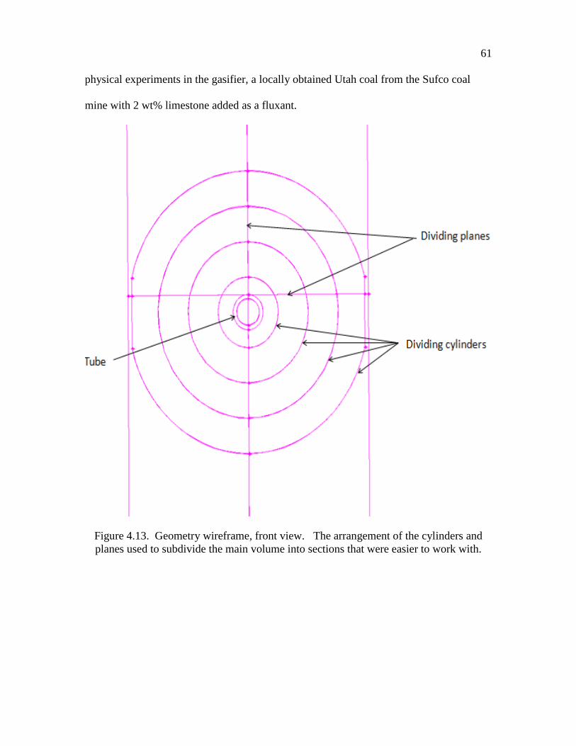
61
physical experiments in the gasifier, a locally obtained Utah coal from the Sufco coal
mine with 2 wt% limestone added as a fluxant.
Figure 4.13. Geometry wireframe, front view. The arrangement of the cylinders and
planes used to subdivide the main volume into sections that were easier to work with.
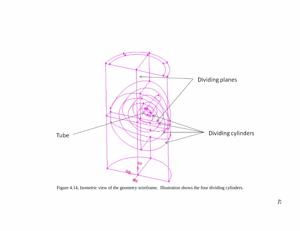
Figure 4.14, Isometric view of the geometry wireframe. Illustration shows the four dividing cylinders.

63
This coal is useful in this instance because it has very low iron content. A great
majority of the slag property models were developed under oxidizing conditions where
the iron is likely to be in the Fe3+
form. However, in a gasification environment, a strong
reducing atmosphere is present and the iron in the slag is more likely to be in the form of
Fe2+
. Studies by Hurley et al. (1996) and Song et al. (2010) both conclude that the
surrounding atmosphere can greatly impact the slag properties, particularly the viscosity.
However, another study by Folkedahl and Schobert (2005) showed that magnitude of the
effect is directly related to the amount of iron in the slag. Due to the different oxidation
states of iron, a low-iron slag is much less affected than a slag with high iron content.
Iron under reducing atmosphere is likely to be in the FeO form. As such, it would
contribute to a weak crystal lattice. Under oxidizing conditions, iron is more likely to be
found in the Fe2O3 form, which with its multiple cross linking capabilities, is more likely
to produce a more cross-linked lattice and, as a result, a more viscous slag. However, due
to the low iron content of the Sufco coal, it was assumed that the models used to describe
the coal properties would be reasonable estimations, despite the difference in the
surrounding atmosphere.
The coal composition was analyzed by Huffman Laboratories (Golden, Colorado,
USA) and their analysis of the mineral matter present is presented in Table 4.2. The
composition of the ash including the 2 wt% limestone fluxant additive is also given in the
table. As can be seen, the amount of iron was 5.25 wt% without the fluxant and only
4.24 wt% after the addition of the limestone.

64
Table 4.2. Ash composition in weight percentage of the Sufco coal. The mass
percentage of each mineral is shown with and without the limestone fluxant additive.
Mineral Original Composition With Limestone Fluxant
SO2 5.96 4.81
SiO2 48.85 39.42
Al2O3 8.34 6.73
CaO 18.21 34.00
FeO 5.25 4.24
MgO 2.84 2.29
Na2O 3.09 2.49
K2O 0.33 0.27
TiO2 0.64 0.52
4.3.2.2 Temperature-independent Properties
The slag density was calculated from eq 3.2, from the work of Mills and Keene,
The heat capacity was calculated using the Kopp-Neumann Law, as given in eq 3.4,
∑
Data for the individual oxide heat capacities were obtained from the Condensed Phase
Thermochemistry Section of the NIST Chemistry Webbook, data compiled by Damalski
and Hearing (2012). Heat capacity values at 1500 K were used when available. When a
specific value at 1500 K wasn’t present in the data, nearby values were linearly
interpolated.
65
Equation 3.5 was used to calculate the thermal conductivity, from the work of
Mills and Rhine,
where and Cp are the values obtained from eqs 3.2 and 3.4. The value for aeff was set to
4.5x10⁻⁷
m2/s, as recommended by Mills and Rhine.
It is possible to calculate the heat capacity, and thereby the thermal conductivity,
based on temperature. However, to do so requires a large amount of effort, expressly
calculating the values as given by the eight-term Shomate equation. For each component,
the eight terms would have to be gathered and the equation recalculated for the given
temperature. Such an effort would have increased computational time and possibly led to
instabilities in the model in exchange for questionable benefit.
4.3.2.3 Viscosity Model
The viscosity model proposed by Senior and Srinivasachar (1995) was applied to
the computational model. This viscosity model was chosen because it is valid over a
wide range of temperatures. Where most models are limited to temperatures above the
Tcv of the slag, the model developed by Senior and Srinivasachar has a separate equation
for predicting the slag viscosity in the high-viscosity region below the Tcv. It was
postulated that in a computational model, the greatly increased slag viscosity calculated
by the viscosity model could allow the computational model to take the slag freezing into
account without the need to develop an explicit frozen slag layer.

66
The A and B values presented in Section 2.2 were implemented in Eq. 4.5 and
applied to the Fluent simulation by way of a user-defined function or UDF. A UDF is a
short C++ script that is interpreted by Fluent. The UDF used has been included in
Appendix C.
The model was verified by applying it to a similar Sufco slag for which viscosity-
temperature data was available. Groen et al. (1998) collected such data for slag from coal
from the same origin and a very similar mineral composition. After some adjustment of
the parameters, the results were very favorable, shown in Figure 4.15.
4.3.3 Solution Setup
The solution for the model was calculated using the Ansys Fluent package,
version 6.3.26 (Ansys, Canonsberg, Pennsylvania, USA). For each of the geometries, a
steady-state solution was produced using the pressure-based, implicit solver.
To handle the fluid/gas interactions, the implicit volume of fluid (VOF)
multiphase model was selected. According to the Fluent documentation (Fluent Inc.
2006), the VOF model works well for modeling the behavior of two immiscible fluids,
and the user guide suggests that it would work well for jet-breakup and liquid-gas
interface studies. The VOF model is also relatively easy to implement. These strengths
made it an ideal choice for this case.
The Fluent software requires that the PRESTO! discretization method be used for
the pressure calculations with the VOF multiphase model. The momentum calculations
were done using a second-order upwind discretization while the volume fraction
calculations were completed with a first-order upwind discretization scheme. The energy
equation was also discretized using the first-order upwind method.
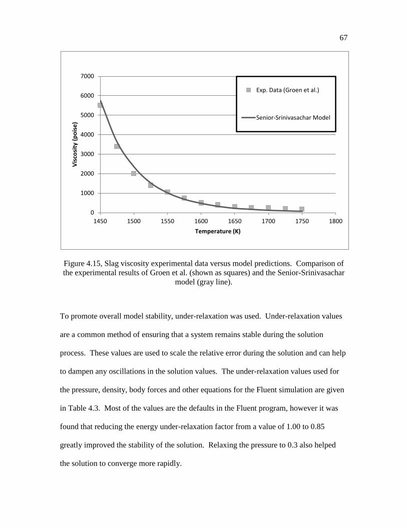
67
Figure 4.15, Slag viscosity experimental data versus model predictions. Comparison of
the experimental results of Groen et al. (shown as squares) and the Senior-Srinivasachar
model (gray line).
To promote overall model stability, under-relaxation was used. Under-relaxation values
are a common method of ensuring that a system remains stable during the solution
process. These values are used to scale the relative error during the solution and can help
to dampen any oscillations in the solution values. The under-relaxation values used for
the pressure, density, body forces and other equations for the Fluent simulation are given
in Table 4.3. Most of the values are the defaults in the Fluent program, however it was
found that reducing the energy under-relaxation factor from a value of 1.00 to 0.85
greatly improved the stability of the solution. Relaxing the pressure to 0.3 also helped
the solution to converge more rapidly.
0
1000
2000
3000
4000
5000
6000
7000
1450 1500 1550 1600 1650 1700 1750 1800
Vis
cosi
ty (
po
ise
)
Temperature (K)
Exp. Data (Groen et al.)
Senior-Srinivasachar Model

68
Table 4.3. Under-relaxation factors used for the computational models. The factors are
used in the solution to promote solution stability.
Equation Under-Relaxation Factor
Pressure 0.3
Density 1.0
Body Forces 1.0
Momentum 0.7
Volume Fraction 0.20
Energy 0.85
4.4 Gasifier Application
4.4.1 Apparatus
4.4.1.1 Reactor
The reactor used for these experiments is a pilot-scale entrained flow gasifier,
located at the University of Utah Gasification Research Facility (Salt Lake City, Utah,
USA). The cylindrical reactor stands approximately 7.3 m in height and has a maximum
thermal input of 600 kWth. This corresponds to a maximum coal feed rate of 70 kg/hr.
The reactor is rated to a maximum pressure of 450 psi (3100 kPa).
A rendering of the gasifier is shown in Figure 4.16. The reactor can be
considered as three distinct functional sections: the insulated reaction section, a pre-
quench section, and the quench section. Fuel and oxidizer are fed into the reaction
section and the product gases and slag move into the pre-quench section. There they are

69
sprayed with water to stop the reactions before passing through the quench bath at the
bottom of the reactor.
The reaction section is 160 cm in length and is refractory lined. The empty
section has a radius of 40.4 cm, but with two, 15.2 cm thick refractory layers, a space
with a radius of 10.2 cm remains for the reactions. The cold face refractory is Plicast
LWI 28 and the hot face refractory is Plicast Si-Bond SP, both from the Plibrico Co.
(Chicago, IL). The cold face is rated at a maximum temperature of 1350 oC and the hot
face refractory is rated to 1760 oC. Both refractory sections consist primarily of Al2O3
and SiO2.
Down the side of the reactor, along the reaction section, are six pairs of opposing
sample ports. Each port is a two-inch (5.1 cm) nominal pipe. The third and fourth sets of
ports, counting from the top, were used for optical access through the reactor.
For coal gasification operations, the reactor is fed coal slurry (an approximately 60 wt%
micronized coal and water mixture) and oxygen. It is downward fired and uses a
concentric two stream burner. In such a burner, the coal slurry is injected through a
small-diameter tube and the oxygen is fed through a surrounding annulus. The velocity
of the oxygen leaving the annulus helps to atomize the coal slurry and increases
conversion.
During operation, the feed rates of the fuel and oxidizer are adjusted to maintain a
set residence time in the reaction section. The coal mass flow rate is governed by
( )
(
(
))
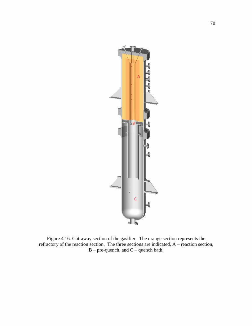
70
Figure 4.16. Cut-away section of the gasifier. The orange section represents the
refractory of the reaction section. The three sections are indicated, A – reaction section,
B – pre-quench, and C – quench bath.

71
where is the residence time, V is the reactor volume, P is the pressure with gage and
atmospheric indicated by g and atm subscripts, is the desired fuel to oxygen ratio, and
is the mole percent of carbon, hydrogen, oxygen, and sulfur in the coal. The equations
used to develop this operation are shown in detail in Appendix E.
4.4.1.2 Gas Jet Diversion Device
Based on the results from the physical and computational models, a jet diversion
device was created to divert the slag inside the operating gasifier. The device consists of
a high-pressure sapphire window, two purge inlets, and a long tube to act as the purge jet.
One purge inlet serves to blow onto the inner surface of the sapphire window to prevent
particulate deposition and to keep water from invading the sight port tube. The other
purge inlet feeds the purge jet to divert the slag. The unit includes a 2-inch, 300 class
flange so that it could be directly mounted to the sample ports on the reactor. Two units
mounted at the same height provide a clear line of sight across the reaction section of the
gasifier. All of these features can be seen in the photograph of the device, shown in
Figure 4.17.
The jet is a simple capillary jet, fashioned from a 5.5 mm OD/4.4 mm ID stainless
steel tube. The length of the tube is approximately 33mm and is straight for all but the
last 7.5 mm where end of the purge jet tube is angled upward 30o. The tube is oriented so
that it sits suspended along the top of the sight port. From the results of the silicone oil
experiments, it was determined that the optimal point to aim the jet was at the top of the
sight port hole in the refractory. The length of the tube was measured to just sit inside the
hole and direct the jet at that point.

72
Figure 4.17. Jet diversion device. The major features of the device are labeled. The unit
was mounted in the sample port on the gasifier.
The windows were designed and fabricated especially for this project. The
windows are wedge shaped so that the pressure inside the reactor presses the window
further against its seal. This allows the windows to maintain a seal under high pressure
and to maintain that seal even after multiple temperature cycles. The windows sit in a
threaded mount so they can be easily removed for cleaning. A cut away view of the
window design is shown in Figure 4.18.
Each window has two seals. A Teflon gasket sits at the bottom of the threaded
section to provide a seal at the threads. To seal the sapphire piece, the sides of the glass
were coated with Ultra Copper by Permatex (Solon, Ohio), a high-temperature, copper-
infused RTV silicone for making gaskets. A ring of silicone was also deposited around

73
Figure 4.18. Optical access window design. The windows sit in a steel holder that
screws into a base attached to a flange. There are two points for a seal: at the bottom of
the screw down section and between the sapphire and the steel holder. As the pressure in
the reactor increases, the glass presses into the steel holder with greater force, increasing
the strength of the seal. All units are in cm.

74
the perimeter of both ends of the sapphire once it had been inserted into the steel holder.
A photograph of the window holders with the sapphire pieces and silicone seals is shown
Figure 4.19.
4.1.1.3 Alumina Tube Diversion Device
Devices were created to hold an alumina tube in the reaction section of the
gasifier. The device consisted of the body and flange assembly, the window, and the
alumina tube. A single purge inlet blows across the window face to keep any particles
from depositing on the relatively cool sapphire face. Photographs of the completed
assembly are shown in Figures 4.20 – 4.22. The photographs show the tube is held
perpendicular to the flange at the base of the device using a compression fitting scheme.
The fitting was packed with ceramic rope for the compression media. The total tube
length was 47 cm. This length was chosen so that 3.8 cm of the tube penetrated through
the refractory and protruded into the reaction section of the gasifier.
To assemble the device, a small layer of ceramic rope is first coiled into the
retaining hole of the device. Once the ceramic rope has been compacted into the orifice,
the alumina tube is inserted into the center of the rope coil and butted up against the
window section. A steel ring is slipped over the tube and tightened into the retaining
section. The ring compresses the rope and holds the tube tightly in place. No seal is
produced by the rope; however it does cause that the great majority of the purge gas
directed at the inner face of the sapphire travels down the length of the interior of the tube
rather than escaping around the tube exterior. This keeps water and particulates from
making their way into the tube and keeps the device relatively cool during gasifier
operation. The retaining ring and body are shown in Figure 4.21.

75
The windows used for this device were identical to those used in the jet diversion
device. The design works very well in high-temperature and pressure situations and
maintains a seal even after several thermal cycles. A photograph of the complete window
and tube assembly installed on the sight port of the pilot-scale gasifier is shown in Figure
4.22 and a photograph of the complete unit mounted onto the gasifier is shown in Figure
4.23.
Figure 4.19. Steel window holders, sapphire pieces, and the high-temperature silicone
sealant. A fine, 1.25 inch thread was used for the holders. To prevent the parts from
sticking together from the stress of the thermal cycles, the threads were coated with a
nickel-based anti-seize compound, which can also be seen in the photo.

76
Figure 4.20. Assembled alumina tube diversion device.
Figure 4.21. The retaining ring of tube diversion device. The ring compresses ceramic
rope (not pictured) to hold the tube in place and to direct the purge flow down the interior
of the tube.

77
Figure 4.22. Window assembly of tube diversion device. The small white ring seen
through the sapphire is the Teflon seal that sits between the base and the screw down
window holding piece. Also pictured is the purge inlet that directs a stream across the
inner face of the sapphire.

78
Figure 4.23. Mounted assembly of tube diversion device. Photograph of the complete
slag diversion assembly mounted on the gasifier sight port. The orange tint seen in the
window is from the gasifier flame.
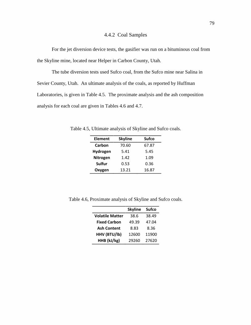
79
4.4.2 Coal Samples
For the jet diversion device tests, the gasifier was run on a bituminous coal from
the Skyline mine, located near Helper in Carbon County, Utah.
The tube diversion tests used Sufco coal, from the Sufco mine near Salina in
Sevier County, Utah. An ultimate analysis of the coals, as reported by Huffman
Laboratories, is given in Table 4.5. The proximate analysis and the ash composition
analysis for each coal are given in Tables 4.6 and 4.7.
Table 4.5, Ultimate analysis of Skyline and Sufco coals.
Element Skyline Sufco
Carbon 70.60 67.87
Hydrogen 5.41 5.45
Nitrogen 1.42 1.09
Sulfur 0.53 0.36
Oxygen 13.21 16.87
Table 4.6, Proximate analysis of Skyline and Sufco coals.
Skyline Sufco
Volatile Matter 38.6 38.49
Fixed Carbon 49.39 47.04
Ash Content 8.83 8.36
HHV (BTU/lb) 12600 11900
HHB (kJ/kg) 29260 27620

80
Table 4.7, Ash composition analysis of Skyline and Sufco coals.
Oxides Skyline Sufco
Aluminum 14.52 8.34
Calcium 6.11 18.21
Iron 5.09 5.25
Magnesium 1.39 2.84
Manganese 0.02 0.05
Phosphorus 0.59 0.01
Potassium 0.57 0.33
Silicon 60.89 48.85
Sodium 1.41 3.09
Sulfur 2.33 5.96
Titanium 0.88 0.64
The NBO/T ratio of the coals is -0.477 for the Skyline sample and 0.395 for the
Sufco sample. The disparity in the non-bridging oxygen ratio is primarily due to the high
amount of calcium present in the Sufco coal. This difference indicates that the slags will
have very different viscosity behaviors when heated.
Each coal was received as a fine pulverized powder (200 mesh). The coal was
mixed with water to create a thick slurry that was approximately 60 wt%.

CHAPTER 5
RESULTS AND DISCUSSION
In this chapter, the results of the physical model, the computational model, and
the gasifier tests are presented and analyzed. The method of data analysis for the
physical model is also developed.
The results are presented in a logical, categorical fashion. However, they were
not performed in the order in which they are presented. The physical model was
developed first. Then, the gasifier test for the jet diversion device was performed. Next,
the computational models were developed and finally the tube diversion device was
applied to the gasifier.
5.1 Silicone Oil Experiments
5.1.1 Jet Diversion Experiments
5.1.1.1 General Observations
The goal of the jet diversion experiments was to determine the effect of film mass
flow rate, film viscosity, jet flow rate, and jet impingement angle on the behavior of the
system.
Figures 5.1-4 show a series of photographs of the film being impacted by the gas
jet. When the jet was applied to the falling oil film at low jet flow rates, it was found that
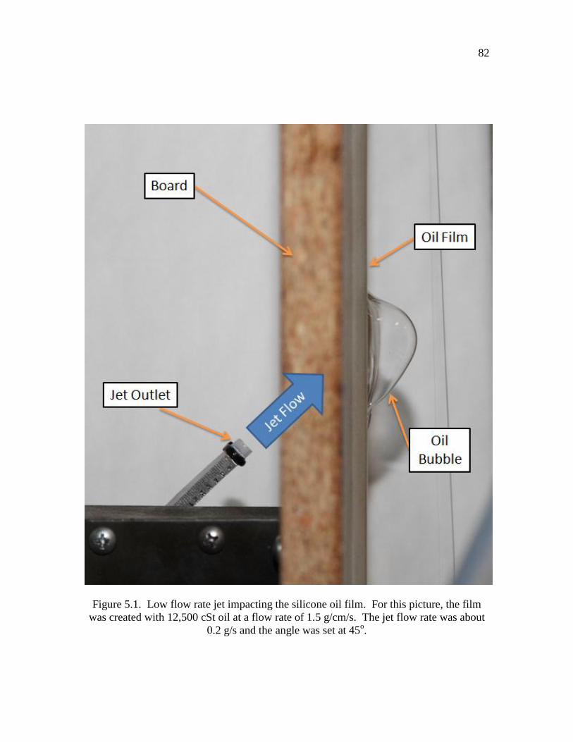
82
Figure 5.1. Low flow rate jet impacting the silicone oil film. For this picture, the film
was created with 12,500 cSt oil at a flow rate of 1.5 g/cm/s. The jet flow rate was about
0.2 g/s and the angle was set at 45o.

83
Figure 5.2. Higher flow gas jet with increased bubble size. This photo is of the same
12,500 cSt film as Figure 5.1 with an increased jet flow rate of 0.25 g/s. The bubble has
pulled even farther away from the film.

84
Figure 5.3. Increased jet flow rate producing a fluctuating bubble. This photograph used
an applied jet flow rate of 0.32 g/s. All other variables are consistent with the previous
photographs. At these conditions, the tip of the bubble would begin to fluctuate up and
down rapidly.

85
Figure 5.4. Silicone oil hood formation. For this photo, the 12,500 cSt silicone oil was
used and the jet was set at 0.24 g/s with a 45o impingement angle. At these conditions,
the hood was stable, but lowering the jet flow rate would cause the hood to fall over the
jet stream and reform the film.

86
the jet would cause a small bubble to form in the face of the film, as shown in Figure 5.1.
The force of the jet impacting the film would cause the film to bulge slightly in the
direction of the jet. The surface of the bubble was stable and did not move unless the jet
flow rate or the film flow rate changed.
Increasing the jet flow rate would cause this bulge to predictably increase in size
and the separation between the film and the bulging shape would become more distinct,
stretching perpendicularly away from the surface of the film. As shown in photograph in
Figure 5.2, while the overall size of the bubble increases, the size of the opening in the
film stays the same.
Further increasing the flow rate of the gas jet would cause the bubble to begin to
fluctuate. The tip of the bubble would drop down and rise up again rapidly. Initially, it
was thought that some of the gas was escaping through the bubble during these
fluctuations and thus some of the pressure on the surface of the bubble was momentarily
relieved. To test this theory, the experiments were repeated with thin strips of paper
placed around the external surface of the bubble to act as a rudimentary method to detect
air currents. It was discovered that no gas passed through the film, despite the erratic
behavior of the bubble. The cause of the bubble’s behavior at this gas flow rate was not
determined, although the effect was repeatable and consistently occurred just before the
bubble would burst. Figure 5.3 shows a photograph of the fluctuating bubble surface.
Increasing the flow rate of the jet any further would cause the bubble to burst
open. Once open, the film would continue to flow around the gas stream, leaving an
open line of sight through the film, even as the jet flow rate was reduced.

87
At the top of the film opening, a lip would be formed. This lip would be stable at
jet flow rates close to that which burst the film initially. As the flow rate was decreased,
it was observed that the lip would destabilize and begin to oscillate away from the wall.
At lower jet flow rates, the lip would stabilize again and form a hood. This hood
formation is shown in Figure 5.4. Soon after this formation was observed, as the jet flow
continued to decrease, the hood would fall over the weakened jet stream and reform a
film. The reformed film is shown in Figure 5.5.
5.1.1.2 Method of Data Interpretation
The precise jet flow rate at which the film burst or closed was recorded for each
of the four viscosities of silicone oil across a range of jet impingement angles. Further
tests using only the 12,500 cSt silicone oil were carried out in which film thickness was
varied by adjusting the film mass flow rate.
It was desired to develop a method of quantifying the effect of each variable (film
viscosity, jet mass flow rate, jet impingement angle, and distance from jet to the film).
To do this, a dimensionless number was developed, similar to the Weber number
discussed in Chapter 2. This dimensionless number, called a Lotte number and noted as
Lo, was intended to provide a ratio of the kinetic energy of the jet to the surface energy of
the film and take each of the previously discussed variables into account. The number
was formulated as

88
Figure 5.5. The reformed oil bubble. In this photograph is 12,500 cSt silicone oil film,
after the gas jet flow rate was decreased to 0.22 g/s. At this flow rate, the hood formation
has dropped across the jet stream and reformed the film.

89
where is the mass flow rate of the gas jet, j is the density of the jet, x is the distance
from the outlet of the jet to the film surface, Af is the impact area of the jet onto the film
surface, and f is the surface tension of the film. Information on the development of this
equation and the calculation of the area of jet impact on the film follows.
The dimensionless number used to analyze the data from the silicone oil
experiments was based on the idea of a Weber number. The Weber number is commonly
used to describe the behavior of droplets on impact with a surface. It is formulated as the
ratio of the kinetic energy of the droplet and the surface energy:
where ρ is the droplet density, D is the droplet diameter, V is the velocity, and γ is the
surface tension.
The Weber number can also be used to measure fluid interactions in other cases
where kinetic forces are important versus surface forces. The concept has been applied to
describe liquid droplet formation in a jet by Senecal (1999) and (Tambe 2004), fluid slag
behavior at a solid interface by Jonsson and Jonsson (1996), and for slag droplet sticking
predictions inside gasifiers by Yu (2010).
For this study, it was found that a formulation similar to the Weber number could
be used to quantify the conditions at which the film burst. The concept of a Weber
number was modified so that, rather than give a ratio of the kinetic energy and surface

90
energy of a single droplet, the new dimensionless number (called a Lotte number, Lo)
would give a measure of the ratio of kinetic energy in the gas jet and the surface energy
of the oil film. Initially this ratio was termed as a modified Weber number. Feedback
from peer review suggested that a new term be created, as the concept is distinct enough
from a traditional Weber number formulation that calling it a Weber number could lead
to confusion.
Due to the constant mass flow of the jet, the kinetic energy was calculated as the
thrust
where is the mass flow rate of the jet and vj is the exit velocity of the gas leaving the
jet. Since the exit velocity of the jet was not measured, the thrust of the jet was based on
the mass flow rate of the jet alone. This was done by using the relation for velocity and
mass flow rate,
where j is the gas density and Aj is the area of the jet. Substituting Eq. F.3 into Eq. F.2
results in

91
The surface energy of the film is the surface tension multiplied by the area of impact of
the jet,
and at the film surface, the area of the jet and area of impact are equal,
where Af is the area of impact of the jet onto the film. The surface energy of the film is
simply the product of the surface tension and the film area,
where f is the surface tension of the film. Dividing the thrust of the jet by the surface
energy results in
A unit analysis of this eq F.8 gives units of inverse length remaining. In order to
remove this remaining unit from the equation, it was desired to remove an area term and
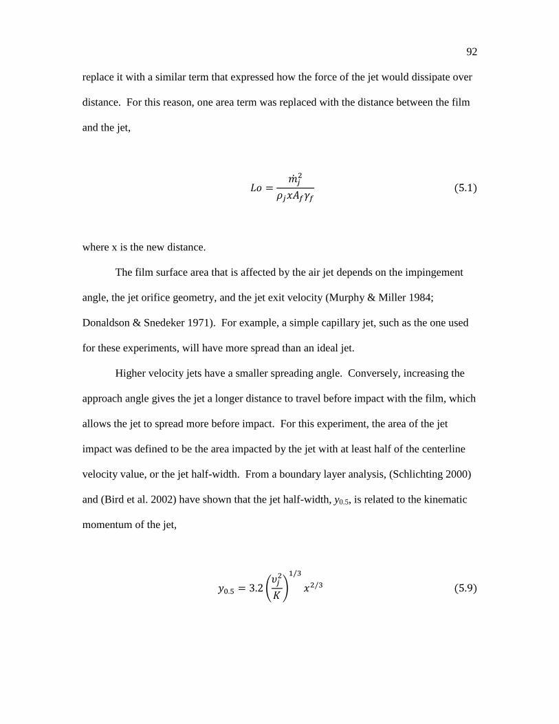
92
replace it with a similar term that expressed how the force of the jet would dissipate over
distance. For this reason, one area term was replaced with the distance between the film
and the jet,
where x is the new distance.
The film surface area that is affected by the air jet depends on the impingement
angle, the jet orifice geometry, and the jet exit velocity (Murphy & Miller 1984;
Donaldson & Snedeker 1971). For example, a simple capillary jet, such as the one used
for these experiments, will have more spread than an ideal jet.
Higher velocity jets have a smaller spreading angle. Conversely, increasing the
approach angle gives the jet a longer distance to travel before impact with the film, which
allows the jet to spread more before impact. For this experiment, the area of the jet
impact was defined to be the area impacted by the jet with at least half of the centerline
velocity value, or the jet half-width. From a boundary layer analysis, (Schlichting 2000)
and (Bird et al. 2002) have shown that the jet half-width, y0.5, is related to the kinematic
momentum of the jet,
(
)

93
where j is the kinematic viscosity of the jet, and K is the kinematic momentum. For a
free jet, the K term can be equated to
where Vjo is the initial jet velocity as the stream exits the jet. Substituting Eq. F.11 in to
Eq. F.10 gives
(
)
The area of the impact of the jet was approximated to be circular, using the half-
width of the jet as the radius. It is noted that the actual impact area would become
increasingly ellipsoidal as the impingement angle increased. However, the difference in
surface area would be relatively small and is ignored in this analysis.
The data points from each experiment were processed into a Lotte number form
so that the results could be easily compared and the effects of each variable could be
determined.
5.1.1.3 Results: Impingement Angle and Viscosity Experiments
Jet flow rate data was collected for a 5 mm thick film of each of the silicone oils.
For each of the oils, the impingement angle of the jet was varied over the range 0-60o and
the jet flow rates at which the film would burst and reclose were noted.

94
In the case of the 100 cSt oil, no data could be collected for impingement angles
less than 30o. Lower impingement angles resulted in the oil spattering to such a degree
that an accurate assessment of when the film burst or closed was not possible.
Figure 5.6 shows the jet flow rate at which the film burst versus the impingement
angle. Four series of data are shown, one for each of the oil viscosities. Several data
points were collected for each configuration, but for easy interpretation, only the reduced
data is shown in the figure.
Initial examination of the data trend shows that as the impingement angle increases, the
jet flow rate required to burst the film open also increases. However, it is impossible to
determine from the raw data if this increase is due to the physical interaction of the fluids
or the changing geometry. Converting these data to a Lotte number would help to
determine which effects are most responsible for the required flow rate increase.
The data in Figure 5.6 also indicate that some relationship may exist between the
film viscosity and the jet flow rate. Higher viscosity oil films appear to generally require
larger jet flow rates to burst.
The data were processed into Lotte number form and again the results were
plotted, as shown in Figure 5.7. When represented in this way, the effects of the change
in geometry, such as the increased jet spread and impact area, are minimized and the
effect of the jet angle can be isolated. From the plot, it appears that the impact angle has
little or no effect on the behavior of the jet and film. The film appears to consistently
burst when the system Lotte number is 4.5-6.0.

95
Figure 5.6. Jet mass flow rate at which the film burst open versus the jet impingement
angle. Different series represent the four different oil viscosities tested. The dashed line
is for a a third-order polynomial regression of the 5,000 cSt oil (R2=0.989), though it
appears to accurately represent the overall trend of all of the oils.
5.1.1.4 Viscosity
When the effect of viscosity is considered, two things stand out in the data. First,
the 12,500 cSt data are remarkably steady across the range of impingement angles,
staying between Lo = 5.2 and 5.5. The data for the 30,000 cSt and 5,000 cSt data are also
very steady, though at different intervals than the 12,500 cSt data. Comparatively, the
data for the 100 cSt has a wider range of Lo = 4.8-5.6. The second interesting feature of
the data is that, discounting the inconsistent 100 cSt results, the trend of higher viscosity
0
0.00005
0.0001
0.00015
0.0002
0.00025
0.0003
0 10 20 30 40 50 60 70
Jet
Flo
w R
ate
(kg
/s)
Impingement Angle (degrees)
100
5k
12.5k
30k

96
Figure 5.7. Lotte number versus impingement angle for film bursting. Data represented
in Figure 5.6 converted into Lotte number form with separate series representing the
different oil viscosities used.
bursting, ranging between Lo = 5.5-6.1. The results of the 12,500 cSt and 5,000 cSt
results follow the trend. However, at the 60o impingement angle, the 100 cSt film burst
at the highest Lotte number. It is possible that the viscosity of the film has a small effect
on the ability of the jet to cause the film to burst. If the viscosity does have such an
effect, it appears to be very slight.
The data for the film closure follow a similar general trend as the data for the film
bursting. In Figure 5.8, the raw jet mass flow rate data for when the film closed is plotted
versus the impingement angle. As before, here the four series each represent a viscosity
of oil. No data was collected for the 100 cSt film for the closure, as the oil’s tendency to
0.0
1.0
2.0
3.0
4.0
5.0
6.0
7.0
0 10 20 30 40 50 60 70
Lott
e N
um
be
r
Impingement Angle (degrees)
100
5k
12.5k
30k

97
break up when impacted with the jet made it difficult to accurately determine when the
film had closed. Similar difficulties were experienced attempting to gather data for the
5,000 cSt silicone oil for impingement angles below 20o.
The data for the film closure show that as the impingement angle increases, the
film is able to close over the jet at higher flow rates. Looking at the effect of viscosity, it
appears that any effect from viscosity becomes more important to the system behavior as
the impingement angle increases. At the higher angles, the data for the three viscosities
is well separated and in decreasing order.
The data points were converted over to a Lotte number form and the results are
shown in Figure 5.9.
When viewed in this form, with the geometric effects removed, it appears that the
impingement angle plays no part in how the jet and film interact. The data appear to be
very consistent across the range of impingement angles with the film closure occurring
when the Lotte number was Lo = 1.4-1.7.
The viscosity effect seen in the film bursting data cannot be seen in the film
closure data. A question arises: if the raw data did show such a strong viscosity trend,
with higher viscosity films able to close at higher jet flow rates, why isn’t this effect
apparent in the Lotte number data? Since the distance from the jet to the film and the
impingement area were consistent across the viscosities, the film closure must be
dominated by the surface tension of the silicone oil. The 30,000 cSt oil had the lowest
surface tension of all, and when this is accounted for, the viscosity effect disappears.

98
Figure 5.8. Jet mass flow rate versus impingement angle for film closure. Data points
represent the jet flow rate at which the oil film closed the diversion versus the
impingement angle of the jet. The displayed trend line is for a third-order polynomial fit
of the data for the 12,500 cSt oil (R2=0.989) and appears to accurately indicate the
general behavior of the other two fluids as well.
Figure 5.9. Lotte number versus the jet impingement angle for film closure. Each series
represents a different oil viscosity.
0
0.00002
0.00004
0.00006
0.00008
0.0001
0.00012
0.00014
0.00016
0.00018
0.0002
0 10 20 30 40 50 60 70
Jet
Mas
s Fl
ow
Rat
e (
kg/s
)
Impingement Angle (degrees)
5k
12.5k
30k
0.0
0.5
1.0
1.5
2.0
2.5
3.0
3.5
4.0
4.5
5.0
0 10 20 30 40 50 60 70
Lott
e N
um
be
r
Impingement Angle (degrees)
5k
12.5k
30k

99
5.1.1.5 Results: Film Thickness Tests
To test the effects of the film thickness on the behavior of the film, experiments
were performed using only the 12,500 cSt oil and a jet impingement angle of 45o and a
variable film mass flow rate. Five film thicknesses were tested between 5.25 and 7.5 mm
and the jet flow rates corresponding to the film bursting and closure were recorded.
The data for the jet flow rate versus the film thickness for both the film burst and
closure are shown in Figure 5.10. Since the film thickness is not accounted for in the
Lotte number, converting the data to this form does not affect the shape of the data.
However, it does allow for easier comparison to previous results. For this reason, the
Lotte number values are displayed in Figure 5.11. As the film thickness is increased, the
jet requires higher flow rates to cause the film to burst. The behavior appears to be
asymptotic with the data points between the 7.0 mm and 7.5 mm film thicknesses all
falling into a very narrow range.
It is interesting to note that as the film thickness increases, the distance between
the film bursting and closure data points lessens before the data approach the asymptotes.
The effect is still present in the Lotte number results, but somewhat more difficult to
distinguish. At the 5.25 mm thickness, the jet flow rate at which the film closes is only
34% of that required to initially burst the film. In the asymptote range, the closure flow
rate is 75% of that required to burst the film.
Figure 5.11 shows the difference between the bursting and closure Lotte numbers.
The actual difference between the two data points at any given film thickness is
surprisingly constant, centering around 3 kg/s. The difference appears to be slightly
higher for the minimum film thickness, but settles into a narrow range as the film

100
Figure 5.10. Jet flow rate versus film thickness for film bursting (diamonds) and closure
(squares).
Figure 5.11. Lotte number versus film thickness. Film bursting is indicated by the
diamonds and closure by the squares. The triangles show the difference between the
bursting Lotte number and the closure Lotte number.
0
0.00005
0.0001
0.00015
0.0002
0.00025
0.0003
0.00035
0.0004
5 5.5 6 6.5 7 7.5 8
Jet
Mas
s Fl
ow
Rat
e (
kg/s
)
Film Thickness (mm)
Closure
Burst
0
2
4
6
8
10
12
14
5 5.5 6 6.5 7 7.5 8
Lott
e N
um
be
r
Film Thickness (mm)
Closure
Burst
Difference

101
thickness increases.
One last observation was that as the film thickness increased, the position of the
diversion relative to the jet outlet would become lower. A hood would be formed where
the jet impacted the film and a thicker film would divert only after travelling a short
distance (about 1-2 cm) farther down the wall.
From these results it appears that it should be possible to divert a slag film around
a sight port with a purge jet. Once a diversion has been established by bursting the slag
film, the diversion could be maintained with a lower purge flow rate.
5.1.2 Alumina Tube Experiments
The experiments involving the alumina tube diversion were performed to gain
qualitative insight rather than quantitative data. Thus only five measurements were
made; one at the expected slag mass flow rate and four more at increasing multiples of
the expected flow rate.
For each experiment, the length of tube required to successfully divert the silicone
oil flow was recorded measured as the length of tube wetted by the oil. The results of the
wetted length measurements are given in Table 5.1. Higher flow rates require longer
lengths of tube to successfully divert the oil flow. The trend appears to be logarithmic, as
shown in Figure 5.12. At the expected slag flow rate, 0.25 g/cm/s, the wetted tube length
was 1.9 cm. When the slag rate was increased to twice that of the expected value, 0.50
g/cm/s, the wetted tube length was increased to 3.0 cm. And at four times the expected
slag flow rate, only 4.5 cm of tube is required to divert the film.

102
Table 5.1, Tube diversion results. First column is the mass flow rate of the oil film. The
second is the ratio of the actual mass flow rate of oil versus the flow rate of slag expected
in the gasifier. The required tube length required to divert the film was recorded in the
third column.
(g/s/cm) Tube Length Wetted by Oil (cm)
0.25 1 1.9
0.375 1.5 3.0
0.5 2 3.8
0.75 3 4.3
1.00 4 4.5
Figure 5.12. Tube length versus oil flow rate. The included trend line is for a
logarithmic regression, R2 = 0.97.
0
0.5
1
1.5
2
2.5
3
3.5
4
4.5
5
0 1 2 3 4 5
Tub
e L
en
gth
(cm
)
Oil/Slag Ratio

103
5.2 Computational Experiments
5.2.1 Model Validation
Before including heat transfer effects, the fluid interaction part of the
computational model was validated by comparing the model predictions to the results of
the silicone oil experiments that had been performed with the jet diversion model.
The computational model was run for four cases that mirrored conditions of the
silicone oil tests. For each case, the computational model was allowed to run for 500
time steps to ensure a steady state solution had been reached. The solution methods and
geometry used were the same as explained in Section 4.2.3.
The first case tested was for a low Lotte number interaction with a thin film.
These conditions are similar to those that were used in the physical model to produce the
photograph shown in Figure 5.1. Figure 5.13 shows the results of the computational
model for these conditions. Specifically for this case, a 12,500 cSt oil with a surface
tension of 19.5 mN/m and a density of 975 kg/m3 was being simulated flowing down a
vertical board. The film mass flow rate was 0.25 g/cm/s to produce a film with a
thickness of 5.5 mm. The mass flow rate of the impinging jet was 0.17 g/s, which
corresponds to a Lotte number of 3.0.
In the physical experiments, these conditions would create a bubble formation but
the bubble would not burst. As can be seen in Figure 5.13, the model predicted the same
behavior. The simulation results show a thin bubble formation with a peak in the same
direction as the jet flow. The second case was identical to the first except that the jet
flow rate was increased to 0.24 g/s which corresponds to a Lotte number of Lo = 8.0.
During the physical experiments, such conditions resulted in the oil film being diverted
104
Figure 5.13. Jet diversion model results for low Lotte number interaction. For this
simulation, conditions were set for a Lo = 3.0 interaction with a film thickness of 5.5
mm. The colors represent the concentration of silicone oil, with light blue representing
the highest concentrations and orange being the lowest. The black lines represent the
wall boundaries of the sight port and the jet.

105
around the jet stream.
The computational results are shown in Figure 5.14. Similar to the effects seen in
the silicone oil tests, the computational model predicts that the diversion occurs right
where the jet impacts the film.
For the third case, the simulation was run to determine how the model would
behave when the thickness of the film was increased. The film flow rate was adjusted to
produce a film thickness of 7.5 mm. In the physical experiments, a Lotte number of 12.5
was required to burst the film of this thickness. A case was run where the Lotte number
was set to Lo = 8.0, which corresponds to a jet flow rate of 0.24 g/s. At these conditions,
it would be expected that the film would form a bubble but not burst. The results are
shown in Figure 5.15. The bubble shape can be clearly seen and, as expected, the film
did not burst in the simulation.
Finally, a case was run with the 7.5 mm film was exposed to an air jet of 0.36 g/s,
which produces a system Lotte number Lo = 13.5. At these conditions, it would be
expected that the film would divert around the jet flow. The results are shown in Figure
15.16. The model does predict that at such conditions, the film would be successfully
diverted. It is also noted that the model predicts a hood to form in the film where it is
impacted by the jet. Also, the point in space at which the film diverts sits slightly lower
relative to the jet outlet than it does for the thinner film thickness case. Both of these
observations are consistent with the results of the physical experiments.
For each of the cases that were run as validation of the Fluent model, the
computation results mirrored the results of the experiments.

106
Figure 5.14, Jet diversion model results for Lo = 8.0. The colors represent the
concentration of silicone oil in the volume, with blue being the highest concentration and
orange representing the lowest. The black line indicate the wall, sight hole, and jet
geometry.

107
Figure 5.15. Jet diversion model results for a high film flow rate with Lo = 8.0. Here the
results for the higher film flow thickness (7.5 mm) is shown for a system Lotte number of
Lo = 8.0. The colors represent the concentration of silicone oil in the given volume with
blue indicating the highest concentrations and orange indicating the lowest. The black
lines represent the sight port and jet geometry. At these conditions a bubble is formed
but the film does not burst, which is consistent with the results of physical
experimentation.

108
Figure 5.16. Jet diversion model results for a high film flow rate with Lo = 13.5. The
model predicts that the film would be successfully diverted at these conditions.

109
5.2.2 Jet Diversion Model
Once the model’s capability of handling the fluid interactions had been
validated, further computational experiments were carried out to determine how heat
transfer effects could impact the ability of a device to divert slag around the sight ports.
The fluid properties were changed to match those of a typical slag based on the Sufco ash
mineral composition. The viscosity was calculated based on the Senior-Srinivasachar
method as discussed in Section 4.2.2.
During the gasifier application tests of the impinging jet method, Skyline coal was
used as the feedstock. The Skyline coal slag has a higher viscosity than the Sufco coal
slag and the results of the computational model using the Sufco slag may not be
immediately applicable. However, the Skyline coal slag could not be modeled as the
Skyline coal NBO/T was less than zero, which is out of the range of the Senior-
Srinivasachar model. Thus the Sufco coal slag was used for both of the methods in the
computational model.
In these simulations, the effects of jet flow rate and temperature on the ability of
the jet diversion system to clear a line of sight through the slag layer were studied. The
initial temperatures of the slag layer, reactor gases, and reactor walls were not changed
for the experiments. Likewise, initial reactor pressure and the flow rates of slag and
reactor gases were also kept constant for each simulation. The values that were used for
each of these variables are based on observed values from gasifier operation with the
values reported in Table 5.2.
The first simulation was designed as a baseline by predicting the results of the jet
diversion when applied to the gasifier at standard operating conditions. The gas jet flow

110
Table 5.2. Conditions for jet diversion simulations. These values were set to be constant
for the duration of the simulation. As the wall temperature was set as a constant, the heat
transfer between the wall and the slag was not reported. More realistic initial slag
temperatures lower than 1900 K were attempted, but the slag would cool too much before
reaching the sight port.
Variable Value Units
Slag Flow Rate 0.25 g/cm/s
Slag Layer Thickness 5.5 mm
Reactor Gas Flow Rate 15 g/s
Slag Initial Temperature 1900 K
Reactor Gases Initial Temperature 2000 K
Reactor Wall Initial Temperature 2000 K
Reactor Pressure 1725 kPa
rate was set at 0.2 g/s, which corresponds to a Lotte number Lo = 5.5. The initial
temperature of the jet was 450 K. The simulation was allowed to run and the results were
examined for every 250 time steps.
The result for the first 250 time steps is shown in Figure 5.17. In this figure, the
cooled slag has begun to form a lip at the top of the sight port at the point where the jet
impinges upon the slag layer. This lip has encroaches slightly into the line of sight. A
large percentage of the sight port is still clear of slag at this point. The remainder of the
slag has just passed the sight port as it flows down the wall, indicating that the simulation
has not reached steady state.
The model was run for 250 more time steps and the results were viewed again,
shown in Figure 5.18. The slag lip has moved further into the line of sight and now
blocks over half of the sight port. At this time step, the cooled slag lip has also begun to

111
Figure 5.17. Results for baseline simulation after 250 time steps. Results of the first
simulation with jet flow rate of 0.2 g/s and initial temperature of 450 K after 250 time
steps as viewed from the front. The colors represent the volume fraction of slag in the
cell with blue being the highest and orange the lowest. Although not shown in this
figure, the volume fraction of slag is 100% along most of the wall above the sight port.
Black lines represent the wall and tube geometry.
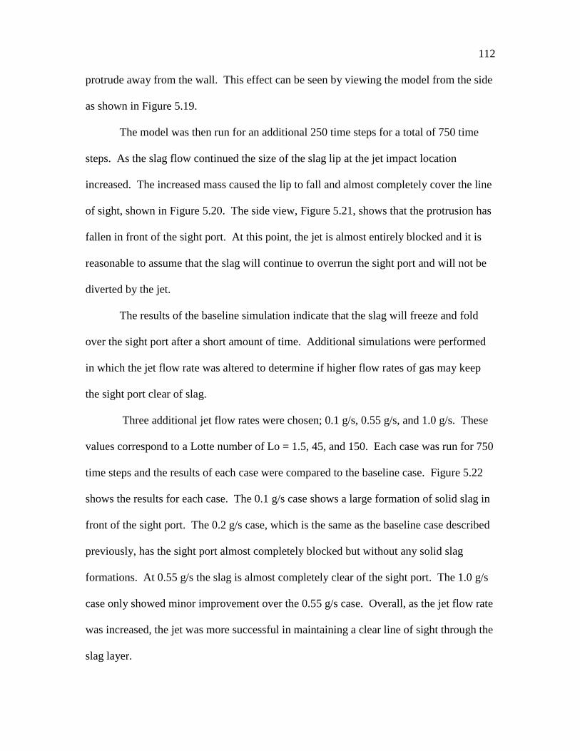
112
protrude away from the wall. This effect can be seen by viewing the model from the side
as shown in Figure 5.19.
The model was then run for an additional 250 time steps for a total of 750 time
steps. As the slag flow continued the size of the slag lip at the jet impact location
increased. The increased mass caused the lip to fall and almost completely cover the line
of sight, shown in Figure 5.20. The side view, Figure 5.21, shows that the protrusion has
fallen in front of the sight port. At this point, the jet is almost entirely blocked and it is
reasonable to assume that the slag will continue to overrun the sight port and will not be
diverted by the jet.
The results of the baseline simulation indicate that the slag will freeze and fold
over the sight port after a short amount of time. Additional simulations were performed
in which the jet flow rate was altered to determine if higher flow rates of gas may keep
the sight port clear of slag.
Three additional jet flow rates were chosen; 0.1 g/s, 0.55 g/s, and 1.0 g/s. These
values correspond to a Lotte number of Lo = 1.5, 45, and 150. Each case was run for 750
time steps and the results of each case were compared to the baseline case. Figure 5.22
shows the results for each case. The 0.1 g/s case shows a large formation of solid slag in
front of the sight port. The 0.2 g/s case, which is the same as the baseline case described
previously, has the sight port almost completely blocked but without any solid slag
formations. At 0.55 g/s the slag is almost completely clear of the sight port. The 1.0 g/s
case only showed minor improvement over the 0.55 g/s case. Overall, as the jet flow rate
was increased, the jet was more successful in maintaining a clear line of sight through the
slag layer.

113
Figure 5.18. Results for baseline simulation after 500 time steps. Results of the first
simulation with jet flow rate of 0.2 g/s and initial temperature of 450 K after 500 time
steps as viewed from the front. The colors represent the volume fraction of slag in the
cell with blue being the highest and orange the lowest. Black lines represent the wall and
tube geometry.

114
Figure 5.19. Results for baseline simulation after 500 time steps, side view. Results of
the first simulation with jet flow rate of 0.2 g/s and initial temperature of 450 K after 500
time steps as viewed from the side. The colors represent the volume fraction of slag in
the cell with blue being the highest and orange the lowest. Black lines represent the wall
and tube geometry.
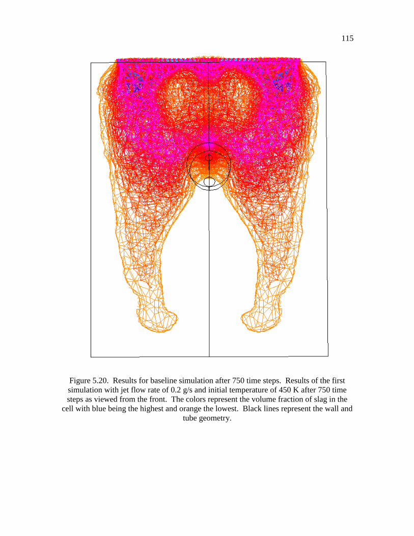
115
Figure 5.20. Results for baseline simulation after 750 time steps. Results of the first
simulation with jet flow rate of 0.2 g/s and initial temperature of 450 K after 750 time
steps as viewed from the front. The colors represent the volume fraction of slag in the
cell with blue being the highest and orange the lowest. Black lines represent the wall and
tube geometry.

116
Figure 5.21. Results for baseline simulation after 750 time steps, side view. Results of
the first simulation with jet flow rate of 0.2 g/s and initial temperature of 450 K after 750
time steps as viewed from the side. The colors represent the volume fraction of slag in
the cell with blue being the highest and orange the lowest. Black lines represent the wall
and tube geometry.

117
Figure 5.22. Results of variable jet simulation. Results of the variable jet flow rate
simulations with jet flow rate of 0.1 g/s (top left), 0.2 g/s (top right), 0.55 g/s (bottom
left), and 1.0 g/s (bottom right) after 750 time steps. The initial temperature of jet was
450 K. The colors represent the volume fraction of slag in the cell with blue being the
highest and orange the lowest. Black lines represent the wall and tube geometry.

118
It was postulated that preheating the jet gas could increase its ability to divert the
slag flow without freezing it. To test this, three tests were run in which the jet gas
temperature was set to 300 K, 450 K, and 600 K. For these tests, the jet flow rate was set
to 0.2 g/s and the simulation was run for 750 time steps.
Screen shots of the results are shown in Figure 5.23. These shots are from the top
of the simulation domain to show how the temperature affected the formation of slag
around the sight port. Each of the cases resulted in a blocked line of sight. However, the
higher temperature cases resulted in much lower amounts of slag build up around the
port. The 300 K case had a very large amount of solid slag build up. In contrast, the 600
K case was clear of slag build up.
From these results, it appears that it is possible to use a gas jet to divert slag inside
a gasifier. However, the amount of gas required is much greater than originally
anticipated. It appears that using 0.55 g/s would sufficient for a line of sight to be
maintained in the reactor. This may not be feasible in a small-scale reactor such as the
one used for this work. At this flow rate, the nitrogen from two jets maintaining an open
line of sight across the reaction section of the gasifier would account for nearly 10% of
the product gas. Such a large amount of diluent would greatly impact the operating
performance of the gasifier. A large-scale gasifier may be able to handle the excess jet
dilution. Such a study could be the subject of a future simulation.

119
Figure 5.23. Result for variable jet temperature simulations. Results of the variable jet
temperature simulations with jet temperature of 300 K (top left), 450 K (top right), and
600 K (bottom) after 750 time steps. The jet flow rate for each case was 0.2 g/s. The
colors represent the volume fraction of slag in the cell with blue being the highest and
orange the lowest. Black lines represent the wall and tube geometry.
Preheating the jet gas did appear to help reduce the amount of slag build up. It is
possible that increasing the purge gas temperature would reduce the amount of gas
required to keep the line of sight clear for long periods of time. Using a combustible gas,
such as methane, as the jet could also be beneficial.
5.2.3 Alumina Tube Model
The tube diversion model uses less than half of the cooling purge gas of the jet
diversion method (0.09 g/s vs. 0.25 g/s). With the alumina tube, the purge stream much

120
lower velocity and empties into the downward-flowing reacting gas without impinging
directly on the slag. For these reasons, it was assumed that the tube model would be less
susceptible to slag freezing issues.
The geometry used for the tube model simulations is discussed in detail in Section
4.2. The simulations performed for the alumina tube model mirrored the experiments
performed using silicone oil. Three simulations were performed; one at the expected slag
flow rate, one at double the expected slag flow rate, and the final at quadruple the
expected slag flow rate. These rates are equal to 0.25 g/s/cm, 0.50 g/s/cm, and 1.00
g/s/cm, respectively. At each flow rate, the flow was of course laminar in behavior with
a very low Reynolds number.
The slag properties, such as density, viscosity, and specific heat, were the same as
those used for the jet diversion simulations. The properties were calculated using the
methods discussed in Section 4.2.2 for a slag composition based on Sufco coal ash. For
this slag, the Tcv, or temperature of critical viscosity, was approximately 1500 K. Any
slag with a temperature below the Tcv would have a very high viscosity and would be
unlikely to flow.
The other model variables were set up to simulate conditions inside the reactor
during normal operation. The values used for the initial temperature of the reactor wall,
the slag layer, the tube, the reacting gases, and the purge gas are given in Table 5.3. Also
included in the table are the reactor gas flow rate, reactor pressure, and the purge gas flow
rate. Each case was run in the steady-state solver for 1500 time steps. The results for
each case were examined every 250 time steps so that changes could be observed
sequentially.

121
Results for each case after 750 time steps are shown in Figures 5.24-26. The results for
the first case, Figure 5.24, show the slag layer flowing around the solid tube Table 5.3.
Conditions used for tube diversion simulations.
Variable Value Units
Reactor Wall Initial Temperature 1900 K
Slag Initial Temperature 1900 K
Tube Initial Temperature 1500 K
Reactor Gases Initial Temperature 2000 K
Purge Gas Initial Temperature 450 K
Reactor Gas Flow Rate 15 g/s
Reactor Pressure 1725 kPa
with a slight thickening of the slag layer as it gathers at the top of the tube. The slag
temperature is lower around the alumina tube and a thin layer of frozen slag has
developed. Slag that accumulates around the tube cools before falling to either side of
the tube. The thickness of the frozen layer remained relatively constant when the
simulation was run for long periods of time.
Figure 5.25 presents the results for the simulation with a slag flow rate of 0.50
g/cm/s. The results are very similar to the 0.25 g/cm/s case in that the slag appears to be
flowing well around the tube. The slight buildup of slag around the tube seen in the first
simulation can also be seen here. There is a large amount of low temperature slag on the
side of the tube. It is likely that this perspective has captured a buildup of cooler slag
around the tube sloughing off.
The third case had a slag flow rate of 1.00 g/s/cm. The results are shown in
Figure 2.26. The slag flow has increased to the point where the tube is no longer able to

122
Figure 5.24. Computational results for first tube simulation. The slag flow rate for this
simulation was 0.25 g/s/cm. In this screen shot the black represents the tube geometry.
The colored lines represent the volume fraction of slag in the cell. The slag layer appears
to flow around the tube.
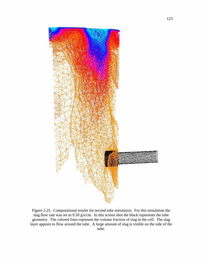
123
Figure 2.25. Computational results for second tube simulation. For this simulation the
slag flow rate was set to 0.50 g/s/cm. In this screen shot the black represents the tube
geometry. The colored lines represent the volume fraction of slag in the cell. The slag
layer appears to flow around the tube. A large amount of slag is visible on the side of the
tube.

124
Figure 5.26. Computational results for third tube simulation. For this simulation the slag
flow rate was set to 1.00 g/s/cm. In this screen shot the black represents the tube
geometry. The colored lines represent the volume fraction of slag in the cell. The slag
layer appears to overwhelming the tube. The slag in front of the tube has begun to cool
in the stream of purge gas.

125
successfully divert the film. The slag has accumulated on the tube and has begun to
encroach into the line of sight. The slag in front of the tube is being cooled by the purge
stream flowing through the tube. Subsequent time steps showed this cooler slag
slumping in front of the tube and cutting off any line of sight through the tube.
The computational model predicts that a heat resistant tube could successfully
divert the slag flow in the reactor even when the slag rate is double the expected rate.
From the results, it also appears that slag freezing is not a major issue in this design. The
only limitation on the application of the design would be the possibility of interference
from the tube in the gasifier operation.
5.3 Gasifier Application
5.3.1 Jet Diversion Device
A series of experiments was performed in August of 2010 in which the jet
diversion device was used in an attempt to maintain a clear line of sight across the
reaction section of the gasifier. Before the gasifier had been operated on coal, the jet
diversion devices discussed in Section 4.3.1 were mounted onto the fourth pair of view
ports from the top of the gasifier.
The devices had been designed so that the tube sits along the top of the sight port.
The tube is bent at the end closest to the reaction section so that the gas jet strikes the slag
stream just as it enters the area of the sight port.
The reactor needed to be prepared before the coal could be gasified. The reactor
was preheated using natural gas until a sufficiently uniform temperature profile had been
established down the length of the reactor. The gas burner was then removed and the

126
coal slurry burner was installed. To continue to increase the temperatures in the reactor,
the gasifier was fired on isopropyl alcohol and oxygen at a slightly substoichiometric
ratio. After approximately 20 minutes of operation on alcohol, the coal slurry feed was
started.
The feed rates of coal slurry and oxygen were adjusted during gasifier operation.
The feed rates were adjusted to maintain a stoichiometric ratio of 0.60. Congruently, the
feed rates were set so that the residence time for the reactants in the gasifier would be 10
seconds. As the pressure in the reactor was increased, the feed rate of the reactants was
adjusted to keep this residence time. Thus as the pressure increased, the overall firing
rate was also increased. During these experiments, the maximum pressure reached was
1725 kPa.
At 1725 kPa reactor pressure, the coal feed rate was 44 kg/hr and the oxygen feed
rate was 71 kg/hr. This corresponds to a firing rate of 1.9 MJ/hr. The approximate slag
flow rate at this rate was 3.68 kg/hr. Assuming an even distribution around the
circumference of the refractory, this equates to 0.031 g/cm/s.
The gas jets were opened as soon as the devices were inserted to protect the metal
from the reactor heat. Initially, while the reactor was operating on natural gas, the rate
was set to 0.10 g/s. This rate was continued while the burner was switched and while the
gasifier ran on isopropyl alcohol.
When the reactor was switched to coal slurry, the jet rate was increased to 0.25
g/s. This rate was intended to keep any slag from running in front of the line of sight.
After 45 minutes of gasifier operation, it was noted that the line of sight had been
compromised. The jet rate was increased to 0.50 g/s in an effort to clear the slag. After
127
an additional 5 minutes at this rate, the sight line across the reactor was still
compromised. The jet rate was further increased to 1.00 g/s, but the slag stayed in place.
Once the reactor was depressurized, the device was removed from the gasifier and
the device and the interior of the sight port were examined. Figure 5.27 shows a
photograph of the device after the experiment. Despite the constant flow of cool gas
through the jet, the metal heated to high enough temperatures to cause serious
degradation to the device. The metal is cracked and flaking.
A photograph taken down the sight port is shown in Figure 5.28. The slag
formation can be seen in the middle of the photograph. The brightest section near the
middle of the frame is the glowing wall of the opposite side of the reactor. The dark
surroundings are the cool sight port tube walls. It appears that slag has crept from the top
and has been frozen into place by the cooling jet. Only a small opening remains in the
lower left section of the sight port.
An attempt was made to remove the slag from the sight port so that optical
measurements could be resumed. A metal rod was inserted into the port, but the slag was
quite solid and would not give. After some time the slag was removed out of the opening
using a hammer.
The formation of the slag in the physical experiments was very similar to what is
predicted by the computational model. The computational model predicted that the slag
layer would be cooled and would slowly slide down to block the line of sight. The results
of the physical experiments uphold the prediction.

128
Figure 5.27. Jet diversion device after use in the gasifier. The damage from heat and
oxidation of the metal can be clearly seen at the tip of the jet.

129
Figure 5.28. View down the sight port after the jet diversion experiments. The brightest
part of the photograph is a view into the reaction section. The slightly darker area just
above is the slag layer that has flowed into the sight line.
5.3.2 Alumina Tube Device
In August of 2011, a campaign of experiments was carried out using the alumina
tube devices to secure optical access to the gasifier. The devices were mounted onto the
third pair of ports down on the gasifier. The devices were used in the reactor for 20 hours
of operation over four days.
Each day of operation, the gasifier was prepared by preheating the reactor by
natural gas combustion. The natural gas was used until a steady temperature distribution
down the reactor interior had been reached, indicating that the refractory had been
sufficiently heated. Then the gas burner was removed and the coal slurry burner was

130
inserted. Isopropyl alcohol was injected with oxygen at a substoichiometric ratio to
continue to drive up the temperatures inside the reactor.
The reactor was operated at a maximum pressure of 280 psi (1930 kPa). The feed
rates of coal slurry and oxygen were adjusted as the pressure increased to maintain a
reactant residence time of 10 seconds. The maximum feed rate of coal slurry during the
experiments was 48 kg/hr and the maximum oxygen feed rate was 78 kg/hr. This feed
rate would generate 4.1 kg/hr of slag. Assuming equal distribution of slag around the
circumference of the inside of the reactor, this would produce 0.035 g/cm/s of slag film
flow.
After each day of operation, the liquid burner was removed and the natural gas
burner was replaced so that the reactor could idle over night. During the swapping of the
burners, the alumina tubes could be seen through the burner port on the top of the reactor.
Photographs of the alumina tubes and slag were taken from this vantage after each day of
operation.
A photograph of the alumina tube after seven hours of gasifier operation is shown
in Figure 5.29. The tube can be clearly seen protruding from the slag layer. The slag
film is flowing around the tube and has only covered a portion of the protrusion. The tip
of the tube does not have any slag on it, so the line of sight remains open through the
reaction section.
At the end of the third day, after eleven hours of gasifier operation, the tubes were
examined again and a crack was discovered in the alumina tube. A photograph of the
cracked tube is shown in Figure 5.30. The fissure is approximately 1 cm long in this
photograph. No problems with the line of sight were reported and so operation continued

131
Figure 5.29. Alumina tube and slag inside the gasifier. This photograph, taken from the
top of the reactor looking down through the feed port, shows the alumina tube protruding
into the reactor. The tube is surrounded by slag and a thick layer has built up at the base
of the protrusion. The tip of the tube remains clean of slag. Large amounts of slag can
be seen in the background of the photo.
132
the next day with the cracked tube in place. The cause of the crack could not be
definitively determined; however possible causes include heat stress, and chemical or
mechanical erosion.
Despite the crack, the line of sight was still open through the tube, so the tube was
left in place. The next day, when the natural gas burner was removed, it was noticed that
the tube was no longer visible. The tip had been destroyed overnight while the gasifier
idled on natural gas. The alumina tube was broken out of the slag layer and replaced with
a fresh tube. No other issues arose with the tubes for the remaining nine hours of the
experiments.
After the experiments, the tubes were broken out of the sight port since the slag
around the tubes had hardened and cemented them into place. The tips of the tubes were
recovered and examined for damage. It was found that the thickness of the tube had been
significantly reduced for the potion that was exposed to the reaction section. A
photograph of a piece of the recovered tube end and a clean, unused alumina tube is
shown in Figure 5.31 for visual comparison. The top of the tube was eroded much more
than the bottom. The top recovered piece of the tube was 1.25 mm thick and bottom was
2.5 mm thick. Original thickness was 3.2 mm.
Overall, the alumina tubes performed very well at diverting the slag film. The
line of sight into the reactor was kept clear of slag for the entire campaign and only one
tube needed to be replaced during the 20 hours of gasification. The results were similar
to the predictions of the computational model for a low slag film flow rate, such as the
one seen in Figure 5.25. However, examination of the tubes after the experiments

133
Figure 5.30. Cracked alumina tube in the gasifier. The crack was noticed during a
burner swap after 11 hours of operation. The crack is small, less than 1 cm in length.
The rest of the tube retained integrity, so the line of sight across the reactor was
preserved.
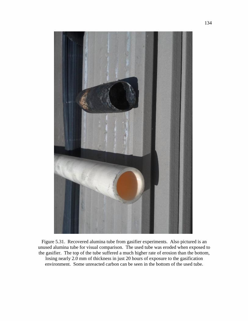
134
Figure 5.31. Recovered alumina tube from gasifier experiments. Also pictured is an
unused alumina tube for visual comparison. The used tube was eroded when exposed to
the gasifier. The top of the tube suffered a much higher rate of erosion than the bottom,
losing nearly 2.0 mm of thickness in just 20 hours of exposure to the gasification
environment. Some unreacted carbon can be seen in the bottom of the used tube.

135
had concluded show that the tips of the tubes that were exposed to the gasification
environment and extreme temperatures of the reactor had high amounts material loss.
The tips lost nearly 2.0 mm of thickness in only 20 hours of operation. This rate of
material loss is similar to that reported by Bakker (1984) for high rates of refractory wear.
This loss was likely due to reactions between the alumina tube and the slag as the fluid
flowed around the tube. Long term application of such a device on a commercial scale
with this material does not seem possible, although improvements in materials or design
may improve performance and durability.
CHAPTER 6
SUMMARY AND CONCLUSIONS
Two methods of diverting a slag film in an entrained-flow coal gasifier were
studied. Physical and computation models were developed in order to understand the
limitations, key parameters, and ideal operating conditions of the slag diversion methods.
From these models, devices were created and successfully tested in a pilot-scale
entrained-flow gasifier.
The first slag diversion method utilized a gas jet to force the slag around a line of
sight. From studying the interaction of a viscous fluid film and an impinging jet, a
dimensionless number was developed to describe the interaction. The number, called the
Lotte number, was based on the Weber number. It is the ratio of the energy of an
impinging jet to the surface energy of the film.
It was found for thin films, the jet will puncture the film if the Lotte number is in
excess of 5.5. The diversion of the film will continue until the jet flow rate has been
reduced to correspond to a Lotte number of 1.5. At this point, the film will fall over the
jet flow and reform a complete film.
Increasing the film thickness results in higher Lotte number flows being required
to pierce the viscous film. The relationship between film thickness and Lotte number is

137
asymptotic, approaching a Lotte number of 12 to pierce thick films and 9.5 to maintain
the film diversion.
The feasibility of using a hollow alumina tube to divert the slag film was also
studied. It was found that as the falling film strikes the side of the tube, the film swells
around the tube and then continues to travel downward. The length of tube protruding
into the reactor to successfully divert the slag flow depended on the thickness of the film.
For the conditions expected in the pilot-scale gasifier, a 4 cm length was determined to be
sufficient.
Computational models of both methods were developed using the Fluent software
package. In both cases, it was desired to examine the effects of heat transfer on the
feasibility of the method to divert the slag flow. Optimal operating conditions for the two
methods were also determined using the computational models.
The model predicted that heat transfer effects would have minimal impact on the
ability of the alumina tube to divert the slag film. However, the model predictions cast
serious doubt on the ability of the jet diversion method to be successful at the assumed
operating conditions. The model predicted that the jet method would freeze a large
amount of slag above the sight port. This mass of slag would eventually fall into the path
of the sight port and would not move, effectively blocking all optical access to the
reactor.
The model did show that preheating the jet gas would have a positive impact on
reducing the amount of slag buildup. Increasing the jet flow rate also resulted in a better
slag diversion. However at the flow rates required to maintain a diversion in the model
would be a serious diluent to the gasifier.

138
Actual application of the devices in the gasifier yielded results very similar to
those of the computational model. The jet diversion method failed to provide an
adequate line of sight after only a short time period of reactor operation and the same
result was predicted even for the lower viscosity Sufco coal slag. On the other hand, the
tube diversion method was very successful at keeping the sight line open even after many
hours of operation. The significant rate of erosion of the alumina tube was the only
concern noted.
For future work it is suggested that attention be given to the possibility of using
frozen slag to provide protection to a solid diversion device, such as the alumina tube. If
an amount of slag could be frozen to the surface of the tube, it would greatly reduce the
tube’s exposure to the erosive slag flow and also to the elevated reactor temperatures.
The jet diversion method may be a viable possibility in a larger scale reactor with
greater heat transfer to the slag layer. Using a different impinging gas such as steam or
recycled syngas could greatly increase the performance of the device without diluting the
reactants. A comprehensive study to optimize the conditions of operation for these gases,
including jet flow rate and preheat temperature could provide interesting insight.
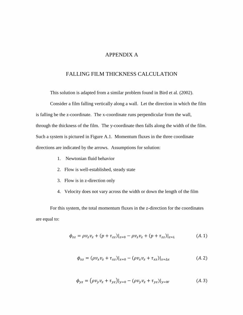
APPENDIX A
FALLING FILM THICKNESS CALCULATION
This solution is adapted from a similar problem found in Bird et al. (2002).
Consider a film falling vertically along a wall. Let the direction in which the film
is falling be the z-coordinate. The x-coordinate runs perpendicular from the wall,
through the thickness of the film. The y-coordinate then falls along the width of the film.
Such a system is pictured in Figure A.1. Momentum fluxes in the three coordinate
directions are indicated by the arrows. Assumptions for solution:
1. Newtonian fluid behavior
2. Flow is well-established, steady state
3. Flow is in z-direction only
4. Velocity does not vary across the width or down the length of the film
For this system, the total momentum fluxes in the z-direction for the coordinates
are equal to:
( )

140
where is the b-direction momentum from the a-direction, and τab is the stress tensor of
b-direction from the a-direction due to viscous interactions, and va is velocity in the
indicated coordinate.
By assuming no velocity in the x- or y-direction, it follows that
Figure A.1. Momentum fluxes

141
Invoking the assumption that the fluid is Newtonian, the shear equations are equal
to
[
] (
)
[
]
[
]
Both of these are zero, since
The sum of the momentum flux must be equal to the forces acting on the volume of the
fluid. In this case, the only force is gravity pulling in the z-direction. The sum of the
momentum can be expressed as

142
where g is the gravitational constant and each momentum flux is multiplied by its
effective area. Again, since the velocity is constant in the z-direction, the second term
may be eliminated. Dividing by x and taking the limit as x →0 results in
Integrating this equation gives
At the surface of the film, x=0, the shear is also zero. Thus C1 is zero.
Now substitution of Newton’s Law of Viscosity, equation A.7, and rearrangement
will yield another equation to be integrated:
Integrating this equation results in
At the opposite boundary condition, at the wall, the velocity is zero. Here x is the
thickness of the film, .

143
[ (
)
]
The mass flow rate of the film can be obtained by integrating this flow rate over the
width and thickness of the film, multiplied by the film density:
∫ ∫
[ (
)
]
which can be arranged to give the thickness as a function of the mass flow rate and the
viscosity.
√

APPENDIX B
MAXIMUM SHEAR RATE OF SILICONE OIL
This exercise proves that the silicone oil used in the physical model behaved as a
Newtonian fluid during the experiments. According to Carré and Woehl (2006), silicone
oil behaves as a Newtonian fluid unless a very high shear rate is applied to the fluid. The
value depends on the viscosity of the fluid; Table B.1 shows the critical shear rate over a
wide range of oil viscosities.
Data regression provides an equation with an R2 value of 0.95,
(
)
where is the kinematic viscosity in cSt. This equation was used to estimate the critical
shear rate for the oils used in this work. These values are presented in Table B.2.
To determine the maximum shear rate experienced by the oil during the
experiments, the maximum shear must first be determined. The greatest shear for the
system as setup in Appendix A is found at the wall/oil interface, where a no-slip
boundary is assumed. In Appendix A it is shown that the shear for any fluid in this
system, be it Newtonian or not, can be expressed as being equal to the density of the fluid
multiplied by the gravitational constant and the thickness of the fluid,

145
Table B.1, Values of critical shear rate for silicone oil. Data provided by Carré and
Woehl.
Viscosity (cSt)
Critical Shear
Rate (s-1
)
1000 18408
2000 6456
5000 1349
10000 1000
60000 275
100000 193
Table B.2. Calculated critical shear rates
Viscosity (cSt)
Critical Shear
Rate (s-1
)
100 105000
5000 1349
12500 1130
30000 495

146
For the system presented here, the maximum shear stress is
The shear rate is defined as
(
)
(
)
where n = 1 for Newtonian fluids. For the fluids used in this work, the greatest shear rate
would be experienced by the least viscous fluid, the 100 cSt oil. Assuming the oil to be
in the Newtonian range, the maximum shear rate for each of the oils can be determined.
The values are presented in Table B.3 with the critical shear rates for comparison. The
calculated values are very small in comparison. It is therefore determined that the
silicone oil did behave as a Newtonian fluid for the experiments performed and detailed
in this work.

147
Table B.3, Critical shear rates and maximum shear rates for the oils used in this work.
Viscosity (cSt)
Critical Shear
Rate (s-1
)
Maximum
Shear
Rate (s-1
)
100 105000 19.5
5000 1349 0.39
12500 1130 0.16
30000 495 0.06

APPENDIX C
SENIOR-SRINIVASACHAR SLAG VISCOSITY MODEL IN UDF FORM
/*********************************************************************
UDF that gives the slag viscosity as a function of temperature. Based on the model
proposed by Senior and Srinivasachar, 1995.
**********************************************************************/
#include "udf.h"
DEFINE_PROPERTY(slag_viscosity,cell,thread)
{
real mu_lam;
real Temp = C_T(cell,thread);
real Tcv = 1050; /* Inflection Temp, Units of Kelvin */
real HighA = -8.698175;
real LowA = -69.93501;
real HighB = 12.026682;
real LowB = 77.663526;
if (Temp > Tcv)
mu_lam = Temp/10 * pow(10, HighA + HighB/(Temp/1000));
else if (Temp < 900)
mu_lam = 100000; /* generates a max viscosity value to avoid overun issues */
else
mu_lam = Temp/10 * pow(10, LowA + LowB/(Temp/1000));;
return mu_lam;
}

APPENDIX D
PENDANT DROP METHOD FOR MEASURING SURFACE TENSION
The pendant drop surface tension measurement technique suspends a droplet of
fluid from a syringe. The device used to conduct these measurements was constructed
and programmed by Vasiliy Chernyshev. By measuring the volume of the droplet and
the contact angle between the droplet and the syringe, the surface tension can be
calculated. An illustration of the technique is shown in Figure 4.7.
In such a system, the force of the surface tension on the droplet is equal to
where Fis the force on the droplet in N, is a constant, d is the tube diameter in m, and
is the surface tension in N/m (Hansen 1991). The amount of surface tension force in the
vertical direction is equal to the force of gravity on the mass of the droplet,
where m is the mass of the droplet in kg, g is the gravitational constant in m/s2, and a is
the contact angle between the droplet and syringe. Replacing the mass of the droplet with
the product of the volume and density and rearranging results in the surface tension,

150
where r is the density in kg/m3 and V is the volume of the droplet in m
3.
For each measurement, a sample of the oil was drawn into a clean syringe. The
syringe was fixed in place perpendicularly with a clamp and the tip of the syringe was
inserted into a transparent, closed chamber. The syringe was depressed until a droplet of
oil hung suspended from the tip of the syringe. A digital camera was aimed at the
transparent chamber and the image was analyzed by a MATLAB program. Photographs
of the syringe, the camera, and the droplet are shown in Figures D.1 and D.2.
The MATLAB program compares the known diameter of the tube to the
boundaries of the droplet to calculate the droplet volume. It also calculates the angle of
contact between the droplet and syringe. With this data, the surface tension of the sample
could be calculated. Between each test, the device was calibrated using water. The
surface tension of the samples averaged 21.1 mN/m and had only slight variation.

151
Figure D.1, Photograph of the surface tension measuring device. Pictured is the syringe,
suspended perpendicularly into a droplet chamber.

152
Figure D.2, Photograph of the droplet chamber with a suspended droplet. In the
background the digital camera used to do the volume analysis of the droplet can be seen.

APPENDIX E
GASIFIER FEED RATE EQUATION DEVELOPMENT
The residence time in the reactor can be defined as
where V is the reactor volume and the dotted V is the volumetric flow rate of the
reactants. Assuming the ideal gas law applies, the volumetric flow can be written as
( )
where the n terms represent the molar flow rate of either carbon (indicated with subscript
C), hydrogen (subscript H), sulfur (subscript S) or oxygen (subscript O). Also, R is the
universal gas constant in proper units, T is the absolute temperature, and Pg is the gage
pressure and Patm is the atmospheric pressure.
The moles of any element, A, fed into the system with the coal stream can be
written as
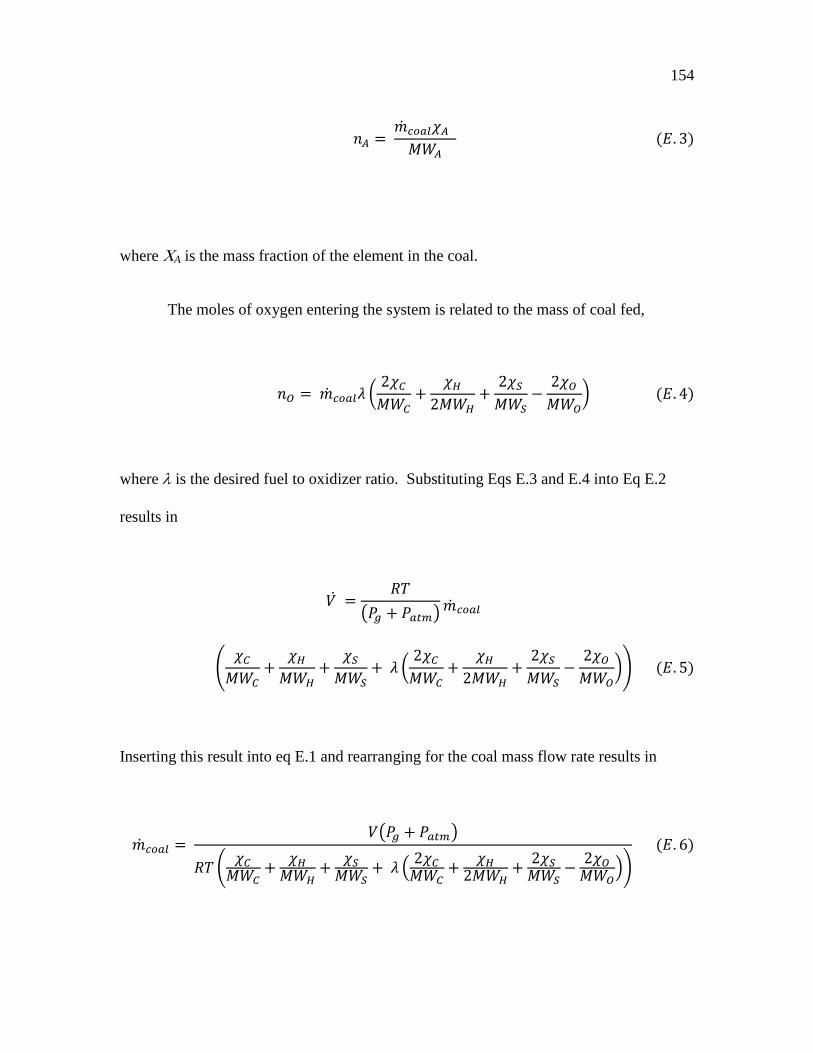
154
where A is the mass fraction of the element in the coal.
The moles of oxygen entering the system is related to the mass of coal fed,
(
)
where is the desired fuel to oxidizer ratio. Substituting Eqs E.3 and E.4 into Eq E.2
results in
( )
(
(
))
Inserting this result into eq E.1 and rearranging for the coal mass flow rate results in
( )
(
(
))

REFERENCES
Aineto, M. et al., 2006. Thermal expansion of slag and fly ash from coal gasification in
IGCC power plant. Fuel, 85(16), pp.2352-2358. Available at:
http://linkinghub.elsevier.com/retrieve/pii/S0016236106001931.
Bakker, W., 1984. Refractory practice in slagging gasifiers. AM. CERAM. SOC. BULL.
Am. Ceram. Soc. Bull. Available at:
http://www.csa.com/partners/viewrecord.php?requester=gs&collection=TRD&
amp;recid=WCA32784WC [Accessed May 5, 2011].
Banks, R.B. & Chandrasekhara, D.V., 1963. Experimental investigation of the
penetration of a high-velocity gas jet through a liquid surface. Journal of Fluid
Mechanics, 15, pp.13-34. Available at:
http://journals.cambridge.org/abstract_S0022112063000021 [Accessed May 5,
2011].
Beer, J., 2007. High efficiency electric power generation: The environmental role.
Progress in Energy and Combustion Science, 33(2), pp.107-134. Available at:
http://linkinghub.elsevier.com/retrieve/pii/S0360128506000347 [Accessed April 6,
2011].
Benyon, P.J., 2002. Computational Modelling of Entrained Flow Slagging Gasifiers.
University of Sydney.
Bird, R.B., Stewart, W.E. & Lightfoot, E.N., 2002. Transport Phenomena 2nd ed.,
Bockelie, M.J. et al., 2001. CFD modeling for entrained flow gasifiers. In Proceedings of
the Gasification Technologies Conference 2002. Citeseer, pp. 28–30. Available at:
http://citeseerx.ist.psu.edu/viewdoc/download?doi=10.1.1.168.1538&rep=rep1
&type=pdf [Accessed May 5, 2011].
Boni, E. & Derge, J., 1956. Surface tensions of silicates. J. Metals.
Bottinga, Y. & Weill, D.F., 1970. Densities of liquid silicate systems calculated from
partial molar volumes of oxide components. American Journal of Science, 269(2),
p.169. Available at: http://www.ajsonline.org/cgi/content/abstract/269/2/169
[Accessed July 27, 2011].
156
Browning, G.J. et al., 2003. An Empirical Method for the Prediction of Coal Ash Slag
Viscosity. Energy & Fuels, 17(3), pp.731-737. Available at:
http://pubs.acs.org/doi/abs/10.1021/ef020165o [Accessed July 24, 2011].
Carré, A. & Woehl, P., 2006. Spreading of silicone oils on glass in two geometries.
Langmuir : the ACS journal of surfaces and colloids, 22(1), pp.134-9. Available at:
http://www.ncbi.nlm.nih.gov/pubmed/16378411.
Clayton, S.J., Stiegel, G.J. & Wimer, J.G., 2002. Gasification Technologies: Gasification
Markets and Technologies — Present and Future - An Industry Perspective,
Cohen, P. & Reid, W., 1944. The Flow of Coal-Ash Slag on Furnace Walls,
Cohen, P. & Reid, W., 1940. Viscosity of Coal Ash Slags. Trans. ASME, 62, pp.141-153.
Damalski, E.S. & Hearing, E.D., 2012. NIST Chemistry Webbook. Condensed Phase
Thermochemistry Data. Available at: http://webbook.nist.gov/chemistry/.
Donaldson, C. & Snedeker, R.S., 1971. A Study of Free Jet Impingement Part 1. Mean
Properties of Free and Impinging Jets.pdf. Journal of Fluid Mechanics, 45(2),
pp.281-326.
Dry, M., 1996. Practical and theoretical aspects of the catalytic Fischer-Tropsch process.
Applied Catalysis A: General, 138(2), pp.319-344. Available at:
http://linkinghub.elsevier.com/retrieve/pii/0926860X95003061.
Duchesne, M. a. et al., 2010. Artificial neural network model to predict slag viscosity
over a broad range of temperatures and slag compositions. Fuel Processing
Technology, 91(8), pp.831-836. Available at:
http://linkinghub.elsevier.com/retrieve/pii/S0378382009003257 [Accessed July 28,
2011].
Van Dyk, J. et al., 2009. Viscosity predictions of the slag composition of gasified coal,
utilizing FactSage equilibrium modelling. Fuel, 88(1), pp.67-74. Available at:
http://linkinghub.elsevier.com/retrieve/pii/S0016236108003050 [Accessed May 5,
2011].
Everard, S., 1949. The History of the Gas Light and Coke Company, London: Ernest
Benn.
Fluent Inc., 2006. Overview and Limitations of the VOF Model. Available at:
http://cdlab2.fluid.tuwien.ac.at/LEHRE/TURB/Fluent.Inc/fluent6.3.26/help/html/ug/
node881.htm.
Folkedahl, B.C., 1997. A Study of the Viscosity of Coal Ash and Slag. Pennsylvania State
University.

157
Folkedahl, B.C. & Schobert, H.H., 2005. Effects of Atmosphere on Viscosity of Selected
Bituminous and Low-Rank Coal Ash Slags. Energy & Fuels, 19(1), pp.208-215.
Available at: http://pubs.acs.org/doi/abs/10.1021/ef040013o.
Frenkel, J., 1955. Kinetic Theory of Liquids, Oxford: Clarendon Press.
Friedman, E.M., 1975. Polymer Viscosity-Molecular Weight Distribution Correlations
via Blending: For High Molecular Weight Poly(dimethyl Siloxanes) and for
Polystyrenes. Journal of Rheology, 19(4), p.493. Available at:
http://link.aip.org/link/?JOR/19/493/1&Agg=doi [Accessed March 16, 2012].
Gohil, D.D. & Mills, K.C., 1981. The Heat Capacity and Enthalpy of Fusion of Slags
Used in Electroslag Remelting. Arch. Eisenhuttenwes., 52(9), pp.335-340.
Grau, A.E. & Masson, C.R., 1976. Densities and molar volumes of silicate melts.
Canadian Metallurgical Quarterly, 15(4), pp.367-374.
Groen, J.. C. et al., 1998. Gasification slag rheology and crystallization in titanium-rich,
iron–calcium–aluminosilicate glasses. Fuel Processing Technology, 56(1-2), pp.103-
127. Available at: http://linkinghub.elsevier.com/retrieve/pii/S0378382098000630.
HANSEN, F., 1991. Surface tension by pendant drop I. A fast standard instrument using
computer image analysis. Journal of Colloid and Interface Science, 141(1), pp.1-9.
Available at: http://linkinghub.elsevier.com/retrieve/pii/002197979190296K
[Accessed March 14, 2012].
Hurley, J.P., Watne, T. & Nowok, J., 1996. The effects of atmosphere and additives on
coal slag viscosity. PREPRINTS OF PAPERS-AMERICAN CHEMICAL SOCIETY
DIVISION FUEL CHEMISTRY, 41, pp.691–694. Available at:
http://www.anl.gov/PCS/acsfuel/preprint archive/Files/41_2_NEW ORLEANS_03-
96_0691.pdf [Accessed May 5, 2011].
Jeffries, J.B., 2009. Tunable Laser Diode Absorption Temperature Measurements in a
Fluidized Bed Gasifier. In Pittsburgh Coal Conference Proceedings.
Jonsson, L. & Jonsson, P., 1996. Modeling face in of Fluid Flow Conditions around the
Slag / Metal Interface in a Gas-stirred Ladle. ISIJ International, 36(d), pp.27-34.
Joseph, D.D., Belanger, J. & Beavers, G.S., 1999. Breakup of a liquid drop suddenly
exposed to a high-speed airstream. International Journal of Multiphase Flow, 25.
Kalmanovitch, D. & Frank, M., 1990. An effective model of viscosity for ash deposition
phenomena. In R. W. Bryers & K. S. Vorres, eds. Mineral Matter and Ash
Deposition from Coal. New York: United Engineering Trustees, Inc.

158
Kondratiev, A. & Jak, E., 2001. Predicting coal ash slag flow characteristics (viscosity
model for the Al2O3–CaO–“FeO”–SiO2 system). Fuel, 80(14), pp.1989-2000.
Available at: http://linkinghub.elsevier.com/retrieve/pii/S0016236101000837.
McDaniel, J., 2002. Tampa Electric Polk Power Station Integrated Gasification
Combined Cycle Project Final Technical Report, Available at:
http://scholar.google.com/scholar?hl=en&btnG=Search&q=intitle:Tampa+Electric+
Polk+Power+Station+Integrated+Gasification+Combined+Cycle+Project+Final+Te
chnical+Report#1 [Accessed May 5, 2011].
Mills, K.C., 1986. Mineral Matter and Ash in Coal. In American Chemical Society
Symposium Series.
Mills, K.C. et al., 2002. Some cautionary notes on the measurement and use of
thermophysical property data. High Temperatures - High Pressures, 34(3), pp.253-
264.
Mills, K.C. & Keene, R.J., 1987. Physical properties of BOS slags. Intl Materials Rev,
32, pp.1-120.
Mills, K.C. & Rhine, J., 1989. The measurement and estimation of the physical properties
of slags formed during coal gasification2. Properties relevant to heat transfer. Fuel,
68(7), pp.904-910. Available at:
http://linkinghub.elsevier.com/retrieve/pii/0016236189901282.
Murphy, H.R. & Miller, D.R., 1984. Effects of Nozzle Geometry on Kinetics in Free-Jet
Expansions. Symposium A Quarterly Journal In Modern Foreign Literatures, 2(2),
pp.4414-4418.
Mysen, B. & Richet, P., 2005. Silicate Glasses and Melts - Properties and Structure,
Elsevier. Available at: http://www.sciencedirect.com/science/book/9780444520111.
Nagabhushana Rao, V. & Ramamurthi, K., 2010. Role of axisymmetric axial velocity
gradients in nonlinear disintegration of liquid sheets. Fluid Dynamics Research,
42(6), p.065505. Available at: http://stacks.iop.org/1873-
7005/42/i=6/a=065505?key=crossref.606daa7f5dd9fdd949a1e02d5cf9077c
[Accessed September 14, 2011].
de Nevers, N., 2005. Fluid Mechanics for Chemical Engineers, New York: McGraw-Hill.
Ni, J. et al., 2010. Molten Slag Flow and Phase Transformation Behaviors in a Slagging
Entrained-Flow Coal Gasifier. Industrial & Engineering Chemistry Research.
Available at: http://pubs.acs.org/doi/abs/10.1021/ie1013844 [Accessed May 5,
2011].
Nicholls, P. & Reid, W., 1940. Viscosity of coal-ash slags. J. Eng. Power, p.12.

159
Oh, M.S. et al., 1995. Effect of crystalline phase formation on coal slag viscosity. Fuel
Processing Technology, 44(1-3), pp.191-199. Available at:
http://linkinghub.elsevier.com/retrieve/pii/037838209500012V.
Ortwein, P. et al., 2010. Absolute diode laser-based in situ detection of HCl in
gasification processes. EXP. FLUIDS, (49), pp.961-968.
Patterson, J.H. et al., 2001. Evaluation of the slag flow characterization of Australian
coals in slagging gasifiers, Newcastle.
Popel, S.I., 1962. Metallurgy of Slags and Their Use in Building. Stell USSR, 67.
Reid, W. & Cohen, P., 1944a. Factors affecting the thickness of coal-ash slag on furnace-
wall tubes. Trans. ASME, 66, pp.685–690. Available at:
http://scholar.google.com/scholar?hl=en&btnG=Search&q=intitle:Factors+Affecting
+the+Thickness+of+Coal-Ash+Slag+on+Furnace-Wall+Tubes#0 [Accessed May 5,
2011].
Reid, W. & Cohen, P., 1944b. The flow characteristics of coal ash slags in the
solidification range. Jour. Eng. Power, Trans. ASME Series A, 66, p.83. Available
at:
http://scholar.google.com/scholar?hl=en&btnG=Search&q=intitle:The+flow+charac
teristics+of+coal-ash+slags+in+the+solidification+range#0 [Accessed July 27,
2011].
Sage, W.L. & McIlroy, J.B., 1959. Relationship of coal ash viscosity to chemical
composition. Combustion, 31(5), pp.41-48.
Sanders, S.T. et al., 2001. Diode-Laser Absorption Sensor for Line-of-Sight Gas
Temperature Distributions. Applied Optics, pp.4404-4015.
Schlichting, H., 2000. Boundary Layer Theory 8th ed., New York: Springer.
Schurch, S., Goerke, J. & Clements, J.A., 1976. Direct Determination of Surface Tension
in the Lung. Proceedings of the National Academy of Sciences, 73(12), pp.4698-
4702. Available at: http://www.pnas.org/cgi/content/abstract/73/12/4698 [Accessed
March 23, 2012].
Seggiani, M., 1998. Modelling and simulation of time varying slag flow in a Prenflo
entrained-flow gasifier. Fuel, 77(14), pp.1611–1621. Available at:
http://linkinghub.elsevier.com/retrieve/pii/S0016236198000751 [Accessed May 5,
2011].
Senecal, P., 1999. Modeling high-speed viscous liquid sheet atomization. International
Journal of Multiphase Flow, 25(6-7), pp.1073-1097. Available at:
http://linkinghub.elsevier.com/retrieve/pii/S0301932299000579.

160
Senior, C.L. & Srinivasachar, S., 1995. Viscosity of Ash Particles in Combustion
Systems for Prediction of Particle Sticking. Energy & Fuels, 9(2), pp.277-283.
Available at: http://pubs.acs.org/doi/abs/10.1021/ef00050a010.
Smith, K.L. et al., 1994. The Structure and Reaction Processes of Coal, New York:
Plenum Press.
Song, W. et al., 2010. Flow properties and rheology of slag from coal gasification. Fuel,
89(7), pp.1709-1715. Available at:
http://linkinghub.elsevier.com/retrieve/pii/S0016236109003421 [Accessed July 25,
2011].
Song, W. et al., 2009. Fusibility and flow properties of coal ash and slag. Fuel, 88(2),
pp.297-304. Available at:
http://linkinghub.elsevier.com/retrieve/pii/S0016236108003499 [Accessed May 5,
2011].
Streeter, R.C., Diehl, E.K. & Schobert, H.H., 1984. The Chemistry of Low Ranked Coals:
Measurement and Prediction of Low-Rank Coal Slag Viscosity, American Chemical
Society.
Sun, K.-H., 1947. FUNDAMENTAL CONDITION OF GLASS FORMATION. Journal
of the American Ceramic Society, 30(9), pp.277-281. Available at:
http://doi.wiley.com/10.1111/j.1151-2916.1947.tb19654.x [Accessed July 28, 2011].
TECO Energy, 2012. TECO Energy - Polk Power Station. Available at:
http://www.tecoenergy.com/news/powerstation/polk/ [Accessed December 3, 2012].
Tambe, S.B., 2004. Liquid Jets in Subsonic Crossflow. Indian Institute of Technology,
Bombay. Available at: http://www.ncbi.nlm.nih.gov/pubmed/20881633.
Urbain, G., 1981. Viscosity of silicate melts. Trans. J. Br. Ceram. Soc., 80, pp.139-141.
Available at:
http://www.csa.com/partners/viewrecord.php?requester=gs&collection=TRD&
amp;recid=WCA21497WC [Accessed May 5, 2011].
Watt, J. & Fereday, F., 1969. The Flow Properties of Slags Formed from the Ashes of
British Coals: Part 1. Viscosity of Homogeneous Liquid Slags in Relation to Slag
Composition. J. Inst. Fuel, 42, pp.99–103. Available at:
http://scholar.google.com/scholar?hl=en&btnG=Search&q=intitle:Flow+properties+
of+slags+formed+from+the+ashes+of+british+coals:+Part+1.+Viscosity+of+homog
eneous+liquid+slags+in+relation+to+slag+composition#0 [Accessed May 5, 2011].
Weymann, H.D., 1962. On the hole theory of viscosity, compressibility, and expansivity
of liquids. Kolloid-Zeitschrift & Zeitschrift fur Polymere, 181(2), pp.131-137.

161
Available at: http://www.springerlink.com/index/10.1007/BF01499664 [Accessed
March 14, 2012].
Yu, G., 2010. A Submodel for Predicting Slag Deposition Formation in Slagging
Gasification Systems. Energy & Fuels.
Zachariasen, W.H., 1932. Characteristics of Glass Formation. Journal of the American
Ceramic Society.
Zbogar, A. et al., 2005. Heat transfer in ash deposits: A modelling tool-box. Progress in
Energy and Combustion Science, 31(5-6), pp.371-421. Available at:
http://linkinghub.elsevier.com/retrieve/pii/S0360128505000249 [Accessed March
15, 2012].
Zhou, X. et al., 2003. Development of a sensor for temperature and water concentration
in combustion gases using a single tunable diode laser. Measurement Science and
Technology, (1459).