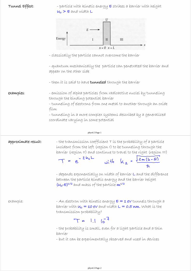
Tunnel Effect: - particle with kinetic energy E strikes a barrier with height U0 > E and width L

- classically the particle cannot overcome the barrier

- quantum mechanically the particle can penetrated the barrier and appear on the other side

- then it is said to have tunneled through the barrier

examples: - emission of alpha particles from radioactive nuclei by tunneling through the binding potential barrier- tunneling of electrons from one metal to another through an oxide film- tunneling in a more complex systems described by a generalized coordinate varying in some potential

phys4.5 Page 1

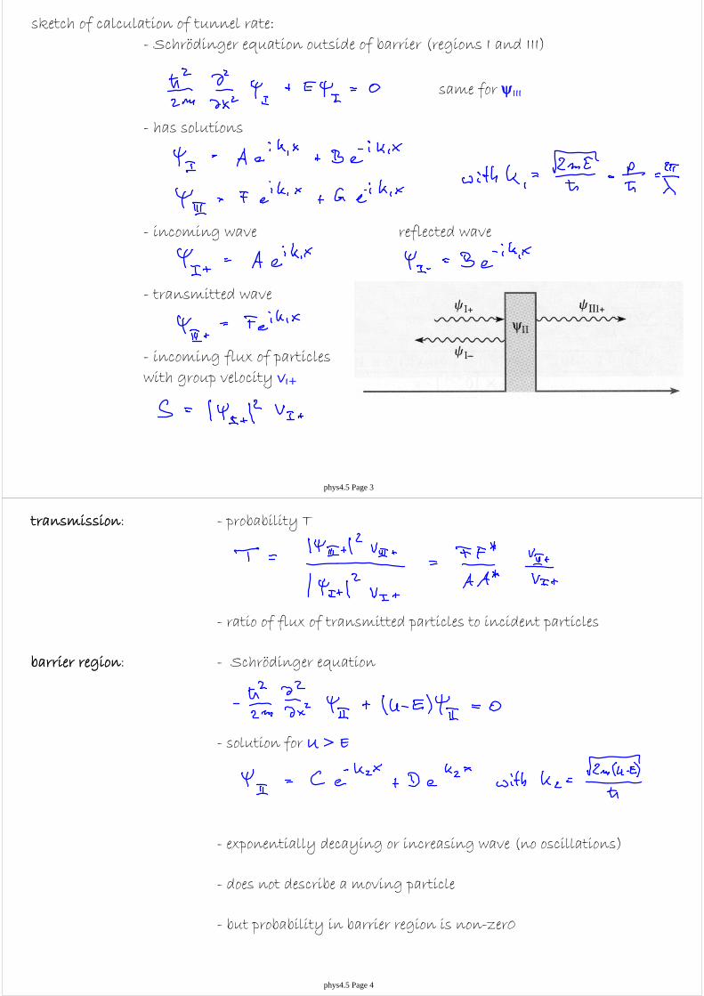
approximate result: - the transmission coefficient T is the probability of a particle incident from the left (region I) to be tunneling through the barrier (region II) and continue to travel to the right (region III)

- depends exponentially on width of barrier L and the difference between the particle kinetic energy and the barrier height (U0-E)1/2 and mass of the particle m1/2

example: - An electron with kinetic energy E = 1 eV tunnels through a barrier with U0 = 10 eV and width L = 0.5 nm. What is the transmission probability?

- the probability is small, even for a light particle and a thin barrier- but it can be experimentally observed and used in devices

phys4.5 Page 2

sketch of calculation of tunnel rate:- Schrödinger equation outside of barrier (regions I and III)

- has solutions

- incoming wave reflected wave

- transmitted wave

- incoming flux of particles with group velocity vI+

same for ψIII

phys4.5 Page 3

transmission: - probability T

- ratio of flux of transmitted particles to incident particles

barrier region: - Schrödinger equation

- solution for U > E

- exponentially decaying or increasing wave (no oscillations)

- does not describe a moving particle

- but probability in barrier region is non-zer0

phys4.5 Page 4

boundary conditions: - at left edge of well (x = 0)

- at right edge of well (X = L)

- solve the four equations for the four coefficients and express them relative to A (|A|2 is proportional to incoming flux)

- solution

phys4.5 Page 5

transmission coefficient: - find A/F from set of boundary condition equations

simplify: - assume barrier U to be high relative to particle energy E

simplify: - assume barrier to be wide (k2L>1)

- therefore

phys4.5 Page 6

transmission coefficient:

- T is exponentially sensitive to width of barrier

- T can be measured in terms of a particle flow (e.g. an electrical current) through a tunnel barrier

- makes this effect a great tool for measuring barrier thicknesses or distances for example in microscopy applications

phys4.5 Page 7

Scanning Tunneling Microscope (STM)

D.M. Eigler, E.K. Schweizer. Positioning single atoms with a STM. Nature 344, 524-526 (1990)

moving individual atoms around one by one

5 nmxenon atoms on a nickel surface

5 nmxenon atoms on a nickel surface

phys4.5 Page 8

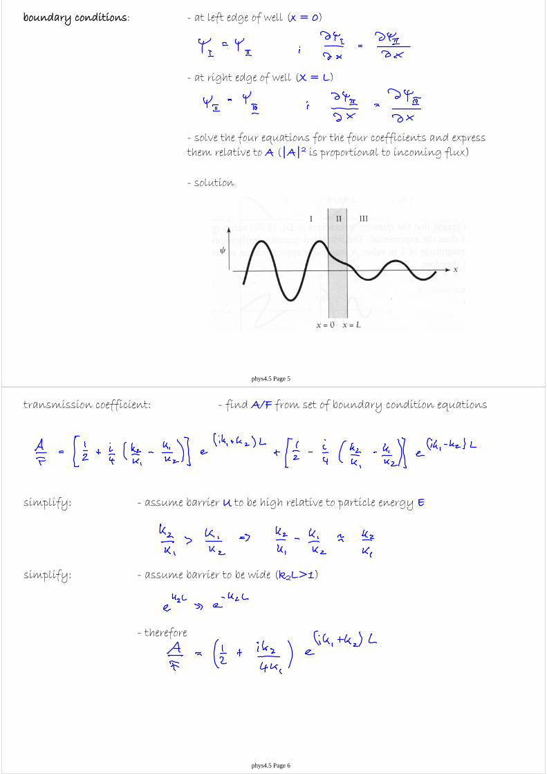
Nobel Prize in Physics (1986)

"for his fundamental work in electron optics, and for the design of the first electron microscope"

"for their design of the scanning tunneling microscope"

IBM Zurich Research Laboratory Rüschlikon, Switzerland

IBM Zurich Research Laboratory Rüschlikon, Switzerland

Fritz-Haber-Institut der Max-Planck-GesellschaftBerlin, Federal Republic of Germany

SwitzerlandFederal Republic of Germany

Federal Republic of Germany

1/4 of the prize1/4 of the prize1/2 of the prize

Heinrich RohrerGerd BinnigErnst Ruska

IBM Zurich Research Laboratory Rüschlikon, Switzerland

IBM Zurich Research Laboratory Rüschlikon, Switzerland

Fritz-Haber-Institut der Max-Planck-GesellschaftBerlin, Federal Republic of Germany

SwitzerlandFederal Republic of Germany

Federal Republic of Germany

1/4 of the prize1/4 of the prize1/2 of the prize

Heinrich RohrerGerd BinnigErnst Ruska

phys4.5 Page 9

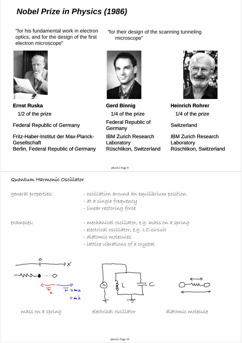
Quantum Harmonic Oscillator

general properties: - oscillation around an equilibrium position- at a single frequency- linear restoring force

examples: - mechanical oscillator, e.g. mass on a spring- electrical oscillator, e.g. LC-circuit- diatomic molecules- lattice vibrations of a crystal

mass on a spring electrical oscillator diatomic molecule

phys4.5 Page 10

- linear restoring force is a prerequisite for harmonic motion- Hooke's law

- equation of motion for harmonic oscillator

- a general solution

- oscillator frequency

equation of motion:

note: - in many physical systems the restoring force is not strictly linear in the oscillation coordinate for large amplitude oscillations- for small oscillation amplitudes however, the harmonic oscillator is usually a good approximation- Taylor expansion of any force about the equilibrium position

phys4.5 Page 11

potential: - potential associated with Hooke's law

- U is used when solving the Schrödinger equation for a harmonic oscillator

expectations: - only a discrete set of energies will be allowed for the oscillator

- the lowest allowed energy will not be E = o but will have some finite value E = E0

- there will be a finite probability for the particle to penetrate into the walls of the potential well

Schrödinger equation for the harmonic oscillator:

phys4.5 Page 12

Solving the harmonic oscillator Schrödinger equation:

rewrite:

normalize:

- these are dimensionless units for the coordinate y and the energy α

- the Schrödinger equation thus is given by

normalization condition for the solution wave functions ψ:

phys4.5 Page 13

energy quantization: - condition on α for normalization

- energy levels of the harmonic oscillator

- equidistant energy levels

- this is a distinct feature of the harmonic oscillator

- zero point energy (n = 0, lowest possible energy of the harmonic oscillator)

phys4.5 Page 14

energy levels in different systems:

constant potential x2 potential 1/r - potentialparticle in a box harmonic oscillator Hydrogen atom

phys4.5 Page 15

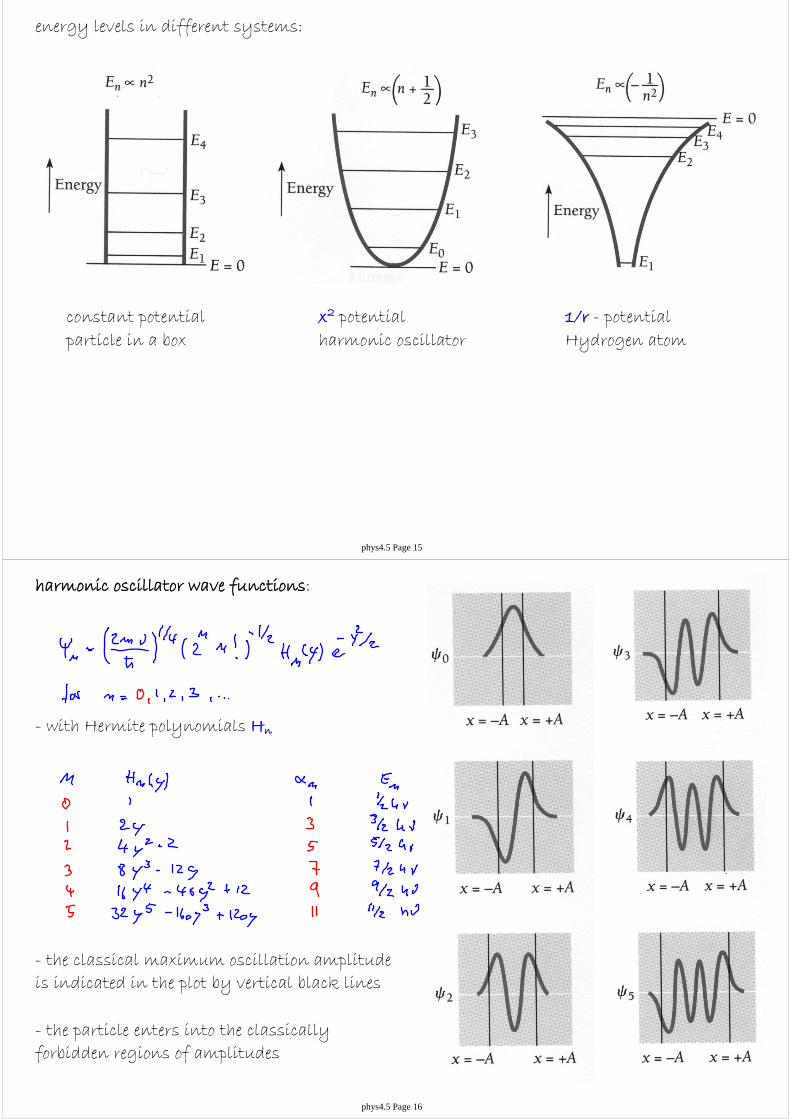
harmonic oscillator wave functions:

- with Hermite polynomials Hn

- the classical maximum oscillation amplitude is indicated in the plot by vertical black lines

- the particle enters into the classically forbidden regions of amplitudes

phys4.5 Page 16

comparison of classical to quantum probability densities of position

classical: - largest probability density at the turningpoints (x = ± a) of the oscillation

quantum: - in the ground state (n = 0) |ψ|2 is largest at theequilibrium position (x = 0)

- for increasing n the quantum probabilitydensity approaches the classical one

- n = 10

- the probability for the quantum oscillator to be at amplitudes larger then ± a decreases for increasing n

- this is an example of the correspondence principle for large n

phys4.5 Page 17

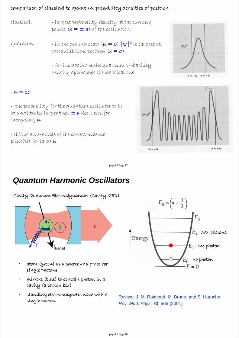
Quantum Harmonic Oscillators

Cavity Quantum Electrodynamics (Cavity QED)

Review: J. M. Raimond, M. Brune, and S. Haroche

Rev. Mod. Phys. 73, 565 (2001)

• atom (green) as a source and probe for single photons

• mirrors (blue) to contain photon in a cavity (a photon box)

• standing electromagnetic wave with a single photon

no photon

one photon

two photons

phys4.5 Page 18

Cavity QEDexperimental setup:

Review: J. M. Raimond, M. Brune, and S. Haroche

Rev. Mod. Phys. 73, 565 (2001)

• O: oven as a source of atoms

• B: LASER preparation stage for atoms

• C: cavity (photon box)

• D: atom detector

one result:

• measurement of probability for atom to be in excited state Pe versus the time ti spend in cavity

• atom probes quantum state (number of photons) in the cavity

phys4.5 Page 19

Quantum HO in Electrical Circuits

sketch of electrical circuit:

• electrical harmonic LC-oscillator

• inductor L

• capacitor C

• electrical artificial atom

• many non-equidistantly spaced energy levels

no photon

one photon

phys4.5 Page 20

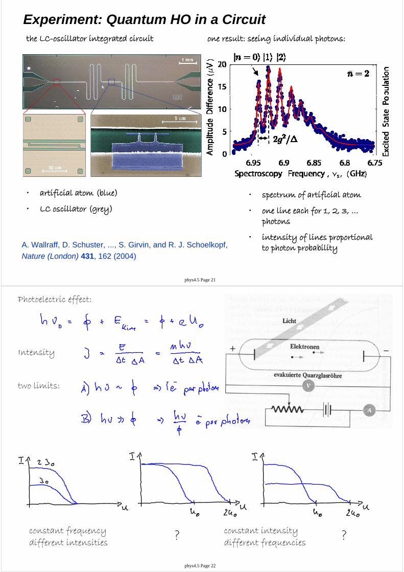
Experiment: Quantum HO in a Circuit

• artificial atom (blue)

• LC oscillator (grey)

A. Wallraff, D. Schuster, ..., S. Girvin, and R. J. Schoelkopf,

Nature (London) 431, 162 (2004)

the LC-oscillator integrated circuit one result: seeing individual photons:

• spectrum of artificial atom

• one line each for 1, 2, 3, …photons

• intensity of lines proportional to photon probability

phys4.5 Page 21

Photoelectric effect:

constant frequencydifferent intensities

constant intensitydifferent frequencies? ?

Intensity

two limits:

phys4.5 Page 22