Minimal Fokker-Planck Theory for the Thermalization of Mesoscopic Subsystems

Igor Tikhonenkov,1 Amichay Vardi,1 James R. Anglin,2 and Doron Cohen3

1Department of Chemistry, Ben Gurion University of the Negev, Beer Sheva 84105, Israel2OPTIMAS Research Center and Fachbereich Physik, Technische Universitat Kaiserslautern, D-67653 Kaiserslautern, Germany

3Department of Physics, Ben Gurion University of the Negev, Beer Sheva 84105, Israel(Received 10 October 2012; published 30 January 2013)

We explore a minimal paradigm for thermalization, consisting of two weakly coupled, low dimensional,

nonintegrable subsystems. As demonstrated for Bose-Hubbard trimers, chaotic ergodicity results in a

diffusive response of each subsystem, insensitive to the details of the drive exerted on it by the other.

This supports the hypothesis that thermalization can be described by a Fokker-Planck equation. We also

observe, however, that Levy-flight type anomalies may arise in mesoscopic systems, due to the wide range

of time scales that characterize ‘sticky’ dynamics.

DOI: 10.1103/PhysRevLett.110.050401 PACS numbers: 05.30.Jp, 03.65.�w, 05.45.Mt, 05.70.Ln

The emergence of irreversibility from reversibleHamiltonian mechanics remains an open fundamentalquestion, even after a century of effort. Recent advancesin computational as well as experimental technique may atlast bring answers within reach. The biggest challenge ofthis quest is the sheer technical difficulty of solving theHamiltonian evolution of quantum many-body systems,even when they are quite small and isolated. In thisLetter, we propose to leap over a significant barrier ofunderstanding, by using Hamiltonian results from a trac-table but nontrivial system, to support an extension of anestablished phenomenological theory, into a substantiallymore challenging regime. The result we thereby derive is asimple theory that can then both guide, and be tested by,subsequent numerical investigations, as well as currentlyfeasible experiments.

We address the thermalization of two nonlinearHamiltonian subsystems that are weakly coupled together,where the combined system is isolated and undriven. Theequilibration of such subsystems is postulated in the zerothlaw of thermodynamics, reflecting the assumption thatmicroscopic dynamics is unobservably fast, while slowermacroscopic dynamics remains nontrivial. Accordingly,weakly coupled subsystems, each having strong internalinteractions, provide the minimal paradigm for the emer-gence of thermodynamics from closed-system mechanics.

Following the Fermi-Pasta-Ulam numerical experiment,most studies of dynamical equilibration have historicallyfocused on large, extended systems [1,2], where the treat-ment of even one strongly interacting system is quiteimpossible in microscopic detail. With experimentalaccess to controlled mesoscopic systems, attention hasmore recently been drawn to thermalization phenomenain small systems, taking into account dynamical chaos[3,4] and quantum effects [5–8]. The traditional analysisof thermalization has nonetheless largely remained withinthe assumptions inherited from the macroscopic problem.It is common to assume that at least one of the two coupled

systems is ‘‘big’’, and hence, can be drastically approxi-mated, either as a phenomenologically described reservoir,or as a time-dependent external parameter. The presentLetter is motivated by the realization that the study ofisolated thermalization of two subsystems is no longer sounthinkably intractable. It is merely extremely difficult.Our proposal is to leverage our understanding of drivenchaotic systems to overcome this difficulty, by viewingeach subsystem as driving the other.The statistical approach.—The statistical description of

driven chaotic systems by means of a Fokker-Planck equa-tion (FPE) for their energy distribution [9–14] is based onthe ergodic adiabatic theorem [15]. Quantum and classicalsystems can be embraced in a unified notation by writingthe energy " as a function of the phase space volume n ofthe constant-energy hypersurface. The density of states isgð"Þ ¼ dn=d" and the microcanonical inverse temperatureis �ð"Þ ¼ d lnðgÞ=d". Upon quantization, the Wigner-Weyl formalism implies that n corresponds to the discreteindex of the energy levels "n, and if these levels are denseenough, they can be approximated as a quasicontinuum.One then makes a coarse-grained description of the slowevolution of the system, and derives an FPE to describethe evolution of the time-dependent energy probabilitydistribution �ð"; tÞ.FPE for a driven system.—If a chaotic system is driven

weakly, its energy changes slowly, and �ð"; tÞ obeys aprobability-conserving FPE, whose diffusion term has acoefficient D, proportional to the strength of the driving[9–11,14]. By Liouville’s theorem, a distribution �ð"Þ /gð�Þ should be a time-independent solution of the FPE.Hence, it is deduced that the drift term in the FPE isuniversally related toD, and the complete phenomenologi-cal equation is established.FPE for coupled subsystems.—We now extend the

single-system FPE phenomenology [9–11] to the caseof thermalization of two subsystems. Each subsystem(i ¼ 1, 2) is characterized by its density of states gið"iÞ

PRL 110, 050401 (2013) P HY S I CA L R EV I EW LE T T E R Sweek ending

1 FEBRUARY 2013

0031-9007=13=110(5)=050401(5) 050401-1 � 2013 American Physical Society

and by its microcanonical inverse temperature �i. Thanksto conservation of energy the thermalization is withinsubspaces of constant energy "1ðn1Þ þ "2ðn2Þ ¼ E.Accordingly, we set "1 ¼ ", and "2 ¼ E � ", and con-struct an FPE for the probability density �ð"; tÞ thatdescribes how the energy is divided between the twosubsystems.

It again follows from Liouville’s theorem that an ergodicdistribution, �ð"Þ / gð"Þ � g1ð"Þg2ðE � "Þ, should be astationary solution. This fixes the form of the FPE, andimplies the functional form of the drift term:

@�

@t¼ @

@"

�gð"ÞDð"Þ @

@"

�1

gð"Þ���

(1)

¼ � @

@"

�Að"Þ�� @

@"½Dð"Þ��

�: (2)

It is important to notice that the diffusion coefficient Dmay depend on ". The optional way, Eq. (2), of writing thisFPE demonstrates that the ‘drift velocity’ A is related to thediffusion as follows:

Að"Þ ¼ @"Dþ ð�1 � �2ÞD: (3)

To see more clearly the connection of Eq. (3) with tradi-tional thermodynamics, assume that each of the subsys-tems is prepared independently in a canonical state, withtemperature Ti, such that gið"iÞ expð�"i=TiÞ describes itsenergy distribution. Integrating both sides of Eq. (3) withthis probability measure, and integrating by parts the firstterm on the right, one obtains [4] a mesoscopic Einsteinrelation, like those previously derived [16,17] usingmaster-equation or fluctuation-theorem approaches:

d

dth"i ¼ hAð"Þi ¼

�1

T1

� 1

T2

�hDi: (4)

This result offers insight into the distinct behaviors ofmicrocanonical energy fluctuations and canonical aver-ages. The canonical version Eq. (4) implies that energyalways flows from the higher to the lower canonical tem-perature, but the more general mesoscopic version Eq. (3)implies that energy flow is not necessarily from the higherto the lower microcanonical temperature and may dependon the functional form ofDð"Þ. This is not in contradictionwith the zeroth law of thermodynamics: energy fluctuatesbetween finite systems in equilibrium such that their aver-age microcanonical temperatures need not be equal. Theergodic solution � / gð"Þ around which Eq. (1) has beenconstructed implies only that the most probable " is the onefor which �1ð"Þ ¼ �2ðE � "Þ.

Fluctuation-dissipation phenomenology.—The deriva-tion of Eq. (1) is phenomenological but based on simpleassumptions that can be tested. Since these include weakcoupling, it is further consistent to compute D using the

Kubo formula. Writing the interaction as H ¼ Qð1ÞQð2Þ,and defining ~SðiÞð!Þ as the power spectrum of the fluctuat-

ing variable QðiÞðtÞ, it reads [18]

D ¼Z 1

0

d!

2�!2 ~Sð1Þð!Þ~Sð2Þð!Þ: (5)

With this addition, the FPE phenomenology provides ageneralized fluctuation-dissipation relation that connectsthe systematic energy flow between the subsystems withthe intensity of the fluctuations.Reasoning.—When two undriven subsystems are

coupled to each other, the effect of one subsystem (call it‘‘agent’’) on the other (call it ‘‘system’’) is like that ofdriving. For the purpose of obtaining Eq. (1), we haveassumed that the interaction results in diffusion that canbe calculated using Eq. (5). Future studies of coupledsystems must test this assumption in full, but one key pointremains to be established with regard to the driven single-subsystem dynamics: The agent-system interaction willtypically couple many quantum levels, even if it is weakin classical terms. In such strongly nonadiabatic circum-stances, energy diffusion, and the applicability of Eq. (5),have not been demonstrated [4]. Below, we complete thisLetter by a numerical demonstration that highlights therole of chaos in obtaining diffusive dynamics for a drivensubsystem, supporting the feasibility of the above reason-ing for experimentally relevant systems.Testing ground.—Few-mode Bose-Hubbard systems are

a promising testing ground, since they are experimentallyaccessible and highly tunable [19], and theoretically trac-table by a wide range of techniques. Since boson number isconserved, their Hilbert spaces are of finite dimension, andyet their classical dynamics can be nonintegrable. Thesmallest Bose-Hubbard system admitting chaos withoutexternal driving is the three-mode trimer [20–26],described by the Bose-Hubbard Hamiltonian (BHH):

H ¼ K

2

Xi¼1;2

ðayi a0 þ ay0aiÞ þU

2

Xi¼0;1;2

ayi ayi aiai; (6)

Here, i ¼ 0, 1, 2 label the three modes, ai and ayi arecanonical destruction and creation operators in secondquantization, K is the hopping frequency, and U is the onsite interaction. The Hamiltonian H commutes with the

total particle number N ¼ Pia

yi ai, and hence, without

loss of generality, we regard N as having a definitevalue N. Driving is then implemented by setting K ¼K0 þ Kd sinð�tÞ. Consequently, the total Hamiltonianhas the structure H 0 þ fðtÞW, where the perturbationoperator W is identified as the first sum in Eq. (6) andthe driving field is fðtÞ ¼ ðKd=2Þ sinð�tÞ.Chaoticity.—The underlying classical dynamics is

defined [4] by replacing the operators ai in theHeisenberg equations of motion [27] with complex c num-bers

ffiffiffiffiffini

pei’i . In the absence of driving, up to trivial rescal-

ing, the classical equations depend only on the singledimensionless parameter u ¼ NU=K0. The chaoticity ofthe motion that is generated by H 0 is reflected in thelocal level statistics and can be quantified by the Brody

PRL 110, 050401 (2013) P HY S I CA L R EV I EW LE T T E R Sweek ending

1 FEBRUARY 2013

050401-2

parameter 0< q< 1 [28], such that q ¼ 0 indicates aPoissonian level-spacing distribution (characteristic ofintegrable dynamics), while higher values indicate theapproach to Wigner level-spacing distribution (indicatingchaotic dynamics).

Figure 1(a) displays the spectrum "n, obtained bynumerical diagonalization of H 0, as a function of u. Forgraphical presentation, we shift and scale the energy spec-trum, for each u, into the same range " 2 ½0; 1�, such that" ¼ 0 and " ¼ 1 are the ground energy E0 and the highestenergy Emax, respectively. By plotting q vs (u, "), as inFig. 1(b), we can identify the " range within which themotion is chaotic at any given value of u. See Ref. [4] fortechnical details. We have verified the implied chaoticityby plotting representative classical Poincare cross sections.

In the numerical simulations, we consider an N ¼ 50particle system with two representative values of u. Thecase u ¼ 5, for which there is a wide chaotic range 0:2<"< 0:6, is contrasted with u ¼ 50, for which the motion isglobally quasi-integrable due to self-trapping.

Energy diffusion.—In the absence of driving, the energyis a constant of motion. Driving induces transitionsbetween energy eigenstates, leading to a time-dependentspread in energy �"ðtÞ. This dispersion is defined as thesquare root of the variance Varð�nÞ that is associated withthe probability distribution

pnðtÞ ¼ jh"nj�ðtÞij2: (7)

In Fig. 2, we plot the time evolution of the quantum energydistribution pnðtÞ in response to driving that is quantummechanically large (many levels are mixed) but classicallysmall (Kd � K0). We contrast the response in the chaotic(u ¼ 5) and in the quasi-integrable (u ¼ 50) regimes.Dramatic differences are observed. In both cases, theenergy distribution in the very early stages of the evolutionreflects the band profile of the perturbation matrixWn;n0 , where n0 is the initial level, as expected from

time-dependent first-order perturbation theory. Later in

the evolution, higher orders of perturbation theory domi-nate. This leads in the quasi-integrable case to Rabi-likeoscillations that have no relation to the classical dynamics.But in the chaotic regime, one observes that the driving iscapable of inducing diffusive-like energy spreading. Thisdiffusive spreading is restricted to the chaotic energy win-dow and features remarkable correspondence with theclassical simulation.Linear response.—The diffusive energy spreading in the

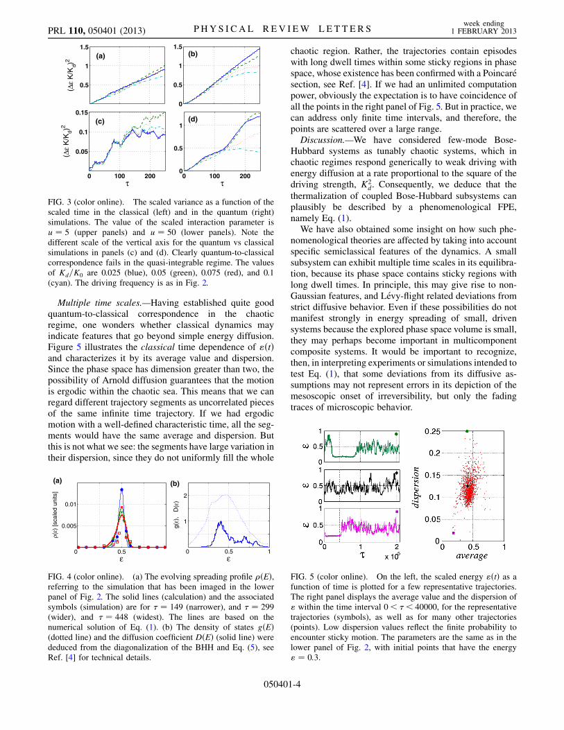
chaotic regime can be quantified by the time evolution ofthe energy variance. In Fig. 3, we plot the time evolution of�" for both the chaotic and the integrable cases. In bothcases, we compare the dispersion obtained under the clas-sical equations of motion for the driven system, startingfrom a microcanonical ensemble, to that obtained fromquantum evolution from an eigenstate with the same en-ergy. As anticipated for diffusive energy spreading, weobserve that in the chaotic regime ð�"Þ2 � 2Dt with dif-fusion coefficient D / K2

d, as assumed in the Kubo linear

response formula Eq. (5).In Fig. 4, we compare the diffusive energy distribution

that is observed in Fig. 2, with the solution of the FPEEq. (1), using the diffusion coefficient from Eq. (5), seeRef. [4] for technical details. The agreement is good,confirming that weakly driven chaotic quantum systemscan indeed exhibit energy diffusion in regimes realistic forexperimental Bose-Hubbard systems and solidifying thebasis of our phenomenological argument for the FPEdescription of intersubsystem equilibration.

0 0.5 1 1.5 2

0.2

0.4

0.6

0.8

log10

(2u)

ε n

0 0.5 1 1.5 2

0.2

0.4

0.6

0.8

log10

(2u)

ε

0

0.2

0.4

0.6

0.8

(b)(a)

FIG. 1 (color online). The energy spectrum of the unperturbedBHH. In panel (a), the scaled eigenenergies "n ofH 0 are plottedvs the scaled interaction parameter, u, for N ¼ 35 particles. Thelevel spacing statistics is characterized by the Brody parameter(0< q< 1), which is displayed in panel (b) for a system withN ¼ 120 particles. In the energy range where the motion ischaotic, q� 1. Square symbols indicate the preparations thatwere used for the simulations in Fig. 2. FIG. 2 (color online). The quantum probability distribution

pnðtÞ for representative simulations is imaged as a function oftime (right). The short-time energy-spreading profile is deter-mined by the perturbation matrix jWn;n0 j2 (left). The number of

particles is N ¼ 50. The upper set is for u ¼ 50 and the lower isfor u ¼ 5. The strength of the driving is Kd=K0 ¼ 0:1. For thetime axis, we use dimensionless units, � ¼ ðEmax � E0Þt=@, andthe scaled driving frequency in both simulations is � � 0:03.The image of the initial level is vertically zoomed and it has theenergy " � 0:5. The boundaries of the chaotic sea in the lowerimage are indicated by the horizontal dashed lines.

PRL 110, 050401 (2013) P HY S I CA L R EV I EW LE T T E R Sweek ending

1 FEBRUARY 2013

050401-3

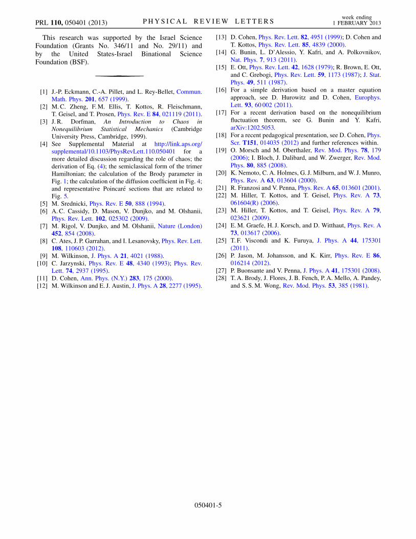
Multiple time scales.—Having established quite goodquantum-to-classical correspondence in the chaoticregime, one wonders whether classical dynamics mayindicate features that go beyond simple energy diffusion.Figure 5 illustrates the classical time dependence of "ðtÞand characterizes it by its average value and dispersion.Since the phase space has dimension greater than two, thepossibility of Arnold diffusion guarantees that the motionis ergodic within the chaotic sea. This means that we canregard different trajectory segments as uncorrelated piecesof the same infinite time trajectory. If we had ergodicmotion with a well-defined characteristic time, all the seg-ments would have the same average and dispersion. Butthis is not what we see: the segments have large variation intheir dispersion, since they do not uniformly fill the whole

chaotic region. Rather, the trajectories contain episodeswith long dwell times within some sticky regions in phasespace, whose existence has been confirmed with a Poincaresection, see Ref. [4]. If we had an unlimited computationpower, obviously the expectation is to have coincidence ofall the points in the right panel of Fig. 5. But in practice, wecan address only finite time intervals, and therefore, thepoints are scattered over a large range.Discussion.—We have considered few-mode Bose-

Hubbard systems as tunably chaotic systems, which inchaotic regimes respond generically to weak driving withenergy diffusion at a rate proportional to the square of thedriving strength, K2

d. Consequently, we deduce that the

thermalization of coupled Bose-Hubbard subsystems canplausibly be described by a phenomenological FPE,namely Eq. (1).We have also obtained some insight on how such phe-

nomenological theories are affected by taking into accountspecific semiclassical features of the dynamics. A smallsubsystem can exhibit multiple time scales in its equilibra-tion, because its phase space contains sticky regions withlong dwell times. In principle, this may give rise to non-Gaussian features, and Levy-flight related deviations fromstrict diffusive behavior. Even if these possibilities do notmanifest strongly in energy spreading of small, drivensystems because the explored phase space volume is small,they may perhaps become important in multicomponentcomposite systems. It would be important to recognize,then, in interpreting experiments or simulations intended totest Eq. (1), that some deviations from its diffusive as-sumptions may not represent errors in its depiction of themesoscopic onset of irreversibility, but only the fadingtraces of microscopic behavior.

0 0.5 1

1

2

ε

g(ε)

, D

(ε)

0 0.5

0.005

0.01

ε

ρ(ε)

[sca

led

units

]

(a) (b)

FIG. 4 (color online). (a) The evolving spreading profile �ðEÞ,referring to the simulation that has been imaged in the lowerpanel of Fig. 2. The solid lines (calculation) and the associatedsymbols (simulation) are for � ¼ 149 (narrower), and � ¼ 299(wider), and � ¼ 448 (widest). The lines are based on thenumerical solution of Eq. (1). (b) The density of states gðEÞ(dotted line) and the diffusion coefficient DðEÞ (solid line) werededuced from the diagonalization of the BHH and Eq. (5), seeRef. [4] for technical details.

0.5

1

1.5

(∆ε

K/K

d)2

0

0.5

1

1.5

0 100 200

0.05

0.1

0.15

τ

(∆ε

K/K

d)2

0 100 2000

0.5

1

τ

(a) (b)

(c) (d)

FIG. 3 (color online). The scaled variance as a function of thescaled time in the classical (left) and in the quantum (right)simulations. The value of the scaled interaction parameter isu ¼ 5 (upper panels) and u ¼ 50 (lower panels). Note thedifferent scale of the vertical axis for the quantum vs classicalsimulations in panels (c) and (d). Clearly quantum-to-classicalcorrespondence fails in the quasi-integrable regime. The valuesof Kd=K0 are 0.025 (blue), 0.05 (green), 0.075 (red), and 0.1(cyan). The driving frequency is as in Fig. 2.

FIG. 5 (color online). On the left, the scaled energy "ðtÞ as afunction of time is plotted for a few representative trajectories.The right panel displays the average value and the dispersion of" within the time interval 0< �< 40000, for the representativetrajectories (symbols), as well as for many other trajectories(points). Low dispersion values reflect the finite probability toencounter sticky motion. The parameters are the same as in thelower panel of Fig. 2, with initial points that have the energy" ¼ 0:3.

PRL 110, 050401 (2013) P HY S I CA L R EV I EW LE T T E R Sweek ending

1 FEBRUARY 2013

050401-4

This research was supported by the Israel ScienceFoundation (Grants No. 346/11 and No. 29/11) andby the United States-Israel Binational ScienceFoundation (BSF).

[1] J.-P. Eckmann, C.-A. Pillet, and L. Rey-Bellet, Commun.Math. Phys. 201, 657 (1999).

[2] M.C. Zheng, F.M. Ellis, T. Kottos, R. Fleischmann,T. Geisel, and T. Prosen, Phys. Rev. E 84, 021119 (2011).

[3] J. R. Dorfman, An Introduction to Chaos inNonequilibrium Statistical Mechanics (CambridgeUniversity Press, Cambridge, 1999).

[4] See Supplemental Material at http://link.aps.org/supplemental/10.1103/PhysRevLett.110.050401 for amore detailed discussion regarding the role of chaos; thederivation of Eq. (4); the semiclassical form of the trimerHamiltonian; the calculation of the Brody parameter inFig. 1; the calculation of the diffusion coefficient in Fig. 4;and representative Poincare sections that are related toFig. 5.

[5] M. Srednicki, Phys. Rev. E 50, 888 (1994).[6] A. C. Cassidy, D. Mason, V. Dunjko, and M. Olshanii,

Phys. Rev. Lett. 102, 025302 (2009).[7] M. Rigol, V. Dunjko, and M. Olshanii, Nature (London)

452, 854 (2008).[8] C. Ates, J. P. Garrahan, and I. Lesanovsky, Phys. Rev. Lett.

108, 110603 (2012).[9] M. Wilkinson, J. Phys. A 21, 4021 (1988).[10] C. Jarzynski, Phys. Rev. E 48, 4340 (1993); Phys. Rev.

Lett. 74, 2937 (1995).[11] D. Cohen, Ann. Phys. (N.Y.) 283, 175 (2000).[12] M. Wilkinson and E. J. Austin, J. Phys. A 28, 2277 (1995).

[13] D. Cohen, Phys. Rev. Lett. 82, 4951 (1999); D. Cohen and

T. Kottos, Phys. Rev. Lett. 85, 4839 (2000).[14] G. Bunin, L. D’Alessio, Y. Kafri, and A. Polkovnikov,

Nat. Phys. 7, 913 (2011).[15] E. Ott, Phys. Rev. Lett. 42, 1628 (1979); R. Brown, E. Ott,

and C. Grebogi, Phys. Rev. Lett. 59, 1173 (1987); J. Stat.

Phys. 49, 511 (1987).[16] For a simple derivation based on a master equation

approach, see D. Hurowitz and D. Cohen, Europhys.

Lett. 93, 60 002 (2011).[17] For a recent derivation based on the nonequilibrium

fluctuation theorem, see G. Bunin and Y. Kafri,

arXiv:1202.5053.[18] For a recent pedagogical presentation, see D. Cohen, Phys.

Scr. T151, 014035 (2012) and further references within.[19] O. Morsch and M. Oberthaler, Rev. Mod. Phys. 78, 179

(2006); I. Bloch, J. Dalibard, and W. Zwerger, Rev. Mod.

Phys. 80, 885 (2008).[20] K. Nemoto, C. A. Holmes, G. J. Milburn, and W. J. Munro,

Phys. Rev. A 63, 013604 (2000).[21] R. Franzosi and V. Penna, Phys. Rev. A 65, 013601 (2001).[22] M. Hiller, T. Kottos, and T. Geisel, Phys. Rev. A 73,

061604(R) (2006).[23] M. Hiller, T. Kottos, and T. Geisel, Phys. Rev. A 79,

023621 (2009).[24] E.M. Graefe, H. J. Korsch, and D. Witthaut, Phys. Rev. A

73, 013617 (2006).[25] T. F. Viscondi and K. Furuya, J. Phys. A 44, 175301

(2011).[26] P. Jason, M. Johansson, and K. Kirr, Phys. Rev. E 86,

016214 (2012).[27] P. Buonsante and V. Penna, J. Phys. A 41, 175301 (2008).[28] T.A. Brody, J. Flores, J. B. Fench, P. A. Mello, A. Pandey,

and S. S.M. Wong, Rev. Mod. Phys. 53, 385 (1981).

PRL 110, 050401 (2013) P HY S I CA L R EV I EW LE T T E R Sweek ending

1 FEBRUARY 2013

050401-5