phy472 advanced quantum mechanics - pieter kok · 5 phy472: advanced quantum mechanics contents 1...
TRANSCRIPT

PHY472
Advanced Quantum MechanicsPieter Kok, The University of Sheffield.
August 2015
PHY472: Lecture Topics
1. Linear vector spaces
2. Operators and the spectral decomposition
3. Observables, projectors and time evolution
4. Tensor product spaces
5. The postulates of quantum mechanics I
6. The postulates of quantum mechanics II
7. The Schrödinger and Heisenberg picture
8. Mixed states and the density matrix
9. Perfect and imperfect measurements
10. Composite systems and entanglement
11. Quantum teleportation
12. Open quantum systems and completely positive maps
13. Orbital angular momentum
14. Spin angular momentum
15. Total angular momentum
16. Identical particles
17. Bose-Einstein and Fermi-Dirac statistics
18. Spin waves in solids
19. An atom in a cavity
20. Quantum field theory
21. Revision lecture (week before the exam)


5
PHY472: Advanced Quantum Mechanics
Contents
1 Linear Vector Spaces and Hilbert Space 71.1 Linear vector spaces . . . . . . . . . . . . . . . . . . . . . . . . . . . . . . . . . . . . . . . 71.2 Operators in Hilbert space . . . . . . . . . . . . . . . . . . . . . . . . . . . . . . . . . . . 81.3 Hermitian and unitary operators . . . . . . . . . . . . . . . . . . . . . . . . . . . . . . . 111.4 Projection operators and tensor products . . . . . . . . . . . . . . . . . . . . . . . . . . 121.5 The trace and determinant of an operator . . . . . . . . . . . . . . . . . . . . . . . . . . 15
2 The Postulates of Quantum Mechanics 18
3 Schrödinger and Heisenberg Pictures 24
4 Mixed States and the Density Operator 294.1 Mixed states . . . . . . . . . . . . . . . . . . . . . . . . . . . . . . . . . . . . . . . . . . . . 294.2 Decoherence . . . . . . . . . . . . . . . . . . . . . . . . . . . . . . . . . . . . . . . . . . . . 314.3 Imperfect measurements . . . . . . . . . . . . . . . . . . . . . . . . . . . . . . . . . . . . 32
5 Composite Systems and Entanglement 375.1 Composite systems . . . . . . . . . . . . . . . . . . . . . . . . . . . . . . . . . . . . . . . . 375.2 Entanglement . . . . . . . . . . . . . . . . . . . . . . . . . . . . . . . . . . . . . . . . . . . 375.3 Quantum teleportation . . . . . . . . . . . . . . . . . . . . . . . . . . . . . . . . . . . . . 41
6 Evolution of Open Quantum Systems 446.1 The Lindblad equation . . . . . . . . . . . . . . . . . . . . . . . . . . . . . . . . . . . . . 446.2 Positive and completely positive maps . . . . . . . . . . . . . . . . . . . . . . . . . . . . 45
7 Orbital Angular Momentum and Spin 477.1 Orbital angular momentum . . . . . . . . . . . . . . . . . . . . . . . . . . . . . . . . . . 477.2 Spin . . . . . . . . . . . . . . . . . . . . . . . . . . . . . . . . . . . . . . . . . . . . . . . . . 497.3 Total angular momentum . . . . . . . . . . . . . . . . . . . . . . . . . . . . . . . . . . . . 527.4 Composite systems with angular momentum . . . . . . . . . . . . . . . . . . . . . . . . 53
8 Identical Particles 578.1 Symmetric and anti-symmetric states . . . . . . . . . . . . . . . . . . . . . . . . . . . . 578.2 Creation and annihilation operators . . . . . . . . . . . . . . . . . . . . . . . . . . . . . 588.3 Observables based on creation and annihilation operators . . . . . . . . . . . . . . . . 628.4 Bose-Einstein and Fermi-Dirac statistics . . . . . . . . . . . . . . . . . . . . . . . . . . 63
9 Many-Body Problems in Quantum Mechanics 669.1 Interacting electrons in atomic shells . . . . . . . . . . . . . . . . . . . . . . . . . . . . . 669.2 Spin waves in solids . . . . . . . . . . . . . . . . . . . . . . . . . . . . . . . . . . . . . . . 689.3 An atom in a cavity . . . . . . . . . . . . . . . . . . . . . . . . . . . . . . . . . . . . . . . 719.4 Outlook: quantum field theory . . . . . . . . . . . . . . . . . . . . . . . . . . . . . . . . . 73

6 PHY472: Advanced Quantum Mechanics
Suggested Further Reading
1. Quantum Processes, Systems, and Information, by Schumacher and Westmoreland,Cambridge University Press (2010). This is an excellent book, and should be your firstchoice for additional material. It has everything up to many-body quantum mechanics.
2. Quantum Information and Quantum Computation, by Nielsen and Chuang, Cam-bridge University Press (2000). This is the current standard work on quantum informationtheory. It has a comprehensive introduction to quantum mechanics along the lines treatedhere, but in more depth. The book is from 2000, which means that several important recenttopics are not covered.
3. Introductory Quantum Optics, by Gerry and Knight, Cambridge University Press (2005).This is a very accessible introduction to the quantum theory of light.
4. Quantum Field Theory, by Lewis Ryder, Cambridge University Press (1996). This is aquite advanced introduction to relativistic quantum field theory.
I would like to thank the students who have used these lecture notes in previous years and spottedtypos or errors (notably Tom Bullock). Their efforts have greatly improved the readability of thesenotes.
c b a n

7
1 Linear Vector Spaces and Hilbert SpaceThe modern version of quantum mechanics was formulated in 1932 by John von Neumann inhis famous book Mathematical Foundations of Quantum Mechanics, and it unifies Schrödingerswave theory with the matrix mechanics of Heisenberg, Born, and Jordan. The theory is framedin terms of linear vector spaces, so the first couple of lectures we have to remind ourselves of therelevant mathematics.
1.1 Linear vector spaces
Consider a set of vectors, denoted by∣∣ψ⟩
,∣∣φ⟩
, etc., and the complex numbers a, b, c, etc. A linearvector space V is a mathematical structure of vectors and numbers that obeys the following rules:
1.∣∣ψ⟩+ ∣∣φ⟩= ∣∣φ⟩+ ∣∣ψ⟩
(commutativity),
2.∣∣ψ⟩+ (
∣∣φ⟩+ ∣∣χ⟩)= (
∣∣ψ⟩+ ∣∣φ⟩)+
∣∣χ⟩(associativity),
3. a(∣∣ψ⟩+ ∣∣φ⟩
)= a∣∣ψ⟩+a
∣∣φ⟩(linearity),
4. (a+b)∣∣ψ⟩= a
∣∣ψ⟩+b∣∣ψ⟩
(linearity),
5. a(b∣∣φ⟩
)= (ab)∣∣φ⟩
.
There is also a null vector 0 such that∣∣ψ⟩+0 =
∣∣ψ⟩, and for every
∣∣ψ⟩there is a vector
∣∣φ⟩such
that∣∣ψ⟩+ ∣∣φ⟩= 0.
For each vector∣∣φ⟩
there is a dual vector⟨φ
∣∣, and the set of dual vectors also form a linearvector space V ∗. There is an inner product between vectors from V and V ∗ denoted by ⟨ψ|φ⟩. Theinner product has the following properties:
1. ⟨ψ|φ⟩ = ⟨φ|ψ⟩∗,
2. ⟨ψ|ψ⟩ ≥ 0,
3. ⟨ψ|ψ⟩ = 0 ⇔∣∣ψ⟩= 0,
4.∣∣ψ⟩= c1
∣∣ψ1⟩+ c2
∣∣ψ2⟩ ⇒ ⟨φ|ψ⟩ = c1⟨φ|ψ1⟩+ c2⟨φ|ψ2⟩,
5. ∥φ∥≡√⟨φ|φ⟩ is the norm of∣∣φ⟩
.
If ∥φ∥= 1, the vector∣∣φ⟩
is a unit vector. The set of unit vectors eiϕ ∣∣ψ⟩ with ϕ ∈ [0,2π) form a
so-called ray in the linear vector space. A linear vector space that has a norm ∥.∥ (there are manydifferent ways we can define a norm) is called a Hilbert space. We will always assume that thelinear vector spaces are Hilbert spaces.
For linear vector spaces with an inner product we can derive the Cauchy-Schwarz inequality,also known as the Schwarz inequality:
|⟨φ|ψ⟩|2 ≤ ⟨ψ|ψ⟩⟨φ|φ⟩ . (1.1)
This is a very important relation, since it requires only the inner product structure. Relations thatare based on this inequality, such as the Heisenberg uncertainty relation between observables,therefore have a very general validity.

8 PHY472: Advanced Quantum Mechanics
If two vectors have an inner product equal to zero, then these vectors are called orthogonal.This is the definition of orthogonality. When these vectors are also unit vectors, they are calledorthonormal. A set of vectors
∣∣φ1⟩,∣∣φ2
⟩,. . .
∣∣φN⟩
are linearly independent if∑j
a j∣∣φ j
⟩= 0 (1.2)
implies that all a j = 0. The maximum number of linearly independent vectors in V is the di-mension of V . Orthonormal vectors form a complete orthonormal basis for V if any vector can bewritten as
∣∣ψ⟩= N∑k=1
ck∣∣φk
⟩, (1.3)
and ⟨φ j|φk⟩ = δ jk. We can take the inner product of∣∣ψ⟩
with any of the basis vectors∣∣φ j
⟩to obtain
⟨φ j|ψ⟩ =N∑
k=1ck⟨φ j|φk⟩ =
N∑k=1
ckδ jk = c j . (1.4)
Substitute this back into the expansion of∣∣ψ⟩
, and we find
∣∣ψ⟩= N∑k=1
∣∣φk⟩⟨φk|ψ⟩ . (1.5)
Therefore∑
k∣∣φk
⟩⟨φk
∣∣ must act like the identity. In fact, this gives us an important clue thatoperators of states must take the general form of sums over objects like
∣∣φ⟩⟨χ∣∣.
1.2 Operators in Hilbert space
The objects∣∣ψ⟩
are vectors in a Hilbert space. We can imagine applying rotations of the vectors,rescaling, permutations of vectors in a basis, and so on. These are described mathematically asoperators, and we denote them by capital letters A, B, C, etc. In general we write
A∣∣φ⟩= ∣∣ψ⟩
, (1.6)
for some∣∣φ⟩
,∣∣ψ⟩ ∈ V . It is important to remember that operators act on all the vectors in Hilbert
space. Let ∣∣φ j
⟩ j be an orthonormal basis. We can calculate the inner product between the
vectors∣∣φ j
⟩and A
∣∣φk⟩:
⟨φ j|(A
∣∣φk⟩)= ⟨φ j|A|φk⟩ ≡ A jk . (1.7)
The two indices indicate that operators are matrices.As an example, consider two vectors, written as two-dimensional column vectors
∣∣φ1⟩= (
10
),
∣∣φ2⟩= (
01
), (1.8)
and suppose that
A =(2 00 3
). (1.9)

Section 1: Linear Vector Spaces and Hilbert Space 9
We calculate
A11 =⟨φ1
∣∣ A∣∣φ1
⟩= (1,0
) ·(2 00 3
)(10
)= (
1,0) ·(2
0
)= 2 . (1.10)
Similarly, we can calculate that A22 = 3, and A12 = A21 = 0 (check this). We therefore have thatA
∣∣φ1⟩= 2
∣∣φ1⟩
and A∣∣φ2
⟩= 3∣∣φ2
⟩.
Complex numbers a have complex conjugates a∗ and vectors∣∣ψ⟩
have dual vectors⟨φ
∣∣. Isthere an equivalent for operators? The answer is yes, and it is called the adjoint, or Hermitianconjugate, and is denoted by a dagger †. The natural way to define it is according to the rule⟨
ψ∣∣ A
∣∣φ⟩∗ = ⟨φ
∣∣ A† ∣∣ψ⟩, (1.11)
for any∣∣φ⟩
and∣∣ψ⟩
. In matrix notation, and given an orthonormal basis ∣∣φ j
⟩ j, this becomes⟨
φ j∣∣ A
∣∣φk⟩∗ = A∗
jk =⟨φk
∣∣ A† ∣∣φ j⟩= A†
k j . (1.12)
So the matrix representation of the adjoint A† is the transpose and the complex conjugate of thematrix A, as given by (A†) jk = A∗
k j. The adjoint has the following properties:
1. (cA)† = c∗A†,
2. (AB)† = B†A†,
3. (∣∣φ⟩
)† = ⟨φ
∣∣.Note the order of the operators in 2: AB is generally not the same as BA. The difference betweenthe two is called the commutator, denoted by
[A,B]= AB−BA . (1.13)
For example, we can choose
A =(0 11 0
)and B =
(1 00 −1
), (1.14)
which leads to
[A,B]=(0 11 0
)(1 00 −1
)−
(1 00 −1
)(0 11 0
)=
(0 −11 0
)−
(0 1−1 0
)=
(0 −22 0
)6= 0 . (1.15)
Many, but not all, operators have an inverse. Let A∣∣φ⟩= ∣∣ψ⟩
and B∣∣ψ⟩= ∣∣φ⟩
. Then we have
BA∣∣φ⟩= ∣∣φ⟩
and AB∣∣ψ⟩= ∣∣ψ⟩
. (1.16)
If Eq. (1.16) holds true for all∣∣φ⟩
and∣∣ψ⟩
, then B is the inverse of A, and we write B = A−1. Anoperator that has an inverse is called invertible. Another important property that an operatormay possess is positivity. An operator is positive if⟨
φ∣∣ A
∣∣φ⟩≥ 0 for all∣∣φ⟩
. (1.17)
We also write this as A ≥ 0.

10 PHY472: Advanced Quantum Mechanics
From the matrix representation of operators you can easily see that the operators themselvesform a linear vector space:
1. A+B = B+ A,
2. A+ (B+C)= (A+B)+C,
3. a(A+B)= aA+aB,
4. (a+b)A = aA+bA,
5. a(bA)= (ab)A.
We can also define the operator norm ∥A∥ according to
∥A∥=√
Tr(A†A)≡√∑
i jA∗
i j A ji , (1.18)
which means that the linear vector space of operators is again a Hilbert space. The symbol Tr(.)denotes the trace of an operator, and we will return to this special operator property later in thissection.
Every operator has a set of vectors for which
A∣∣a j
⟩= a j∣∣a j
⟩, with a j ∈C . (1.19)
This is called the eigenvalue equation (or eigenequation) for A, and the vectors∣∣a j
⟩are the eigen-
vectors. The complex numbers a j are eigenvalues. In the basis of eigenvectors, the matrix repre-sentation of A becomes
A =
a1 0 · · · 00 a2 · · · 0...
... . . . ...0 0 · · · aN
(1.20)
When some of the a js are the same, we speak of degenerate eigenvalues. When there are n iden-tical eigenvalues, we have n-fold degeneracy. The eigenvectors corresponding to this eigenvaluethen span an n-dimensional subspace of the vector space. We will return to subspaces shortly,when we introduce projection operators.
For any orthonormal basis ∣∣φ j
⟩ j we have⟨
φ j∣∣ A
∣∣φk⟩= A jk , (1.21)
which can be written in the form
A =∑jk
A jk∣∣φ j
⟩⟨φk
∣∣ . (1.22)
For the special case where∣∣φ j
⟩= ∣∣a j⟩
this reduces to
A =∑
ja j
∣∣a j⟩⟨
a j∣∣ . (1.23)
This is the spectral decomposition of A. When all a j are equal, we have complete degeneracy overthe full vector space, and the operator becomes proportional (up to a factor a j) to the identity I.

Section 1: Linear Vector Spaces and Hilbert Space 11
Note that this is independent of the basis ∣∣a j
⟩. As a consequence, for any orthonormal basis
∣∣φ j
⟩ we have
I=∑
j
∣∣φ j⟩⟨φ j
∣∣ . (1.24)
This is the completeness relation, and we will use this many times in our calculations.
Lemma: If two non-degenerate operators commute ([A,B] = 0), then they have a common set ofeigenvectors.
Proof: Let A =∑k ak |ak⟩⟨ak| and B =∑
jk B jk∣∣a j
⟩⟨ak|. We can choose this without loss of gener-ality: we write both operators in the eigenbasis of A. Furthermore, [A,B] = 0 implies thatAB = BA.
AB =∑klm
akBlm |ak⟩⟨ak|al⟩⟨am| =∑lm
alBlm |al⟩⟨am|
BA =∑klm
akBlm |al⟩⟨am|ak⟩⟨ak| =∑lm
amBlm |al⟩⟨am| (1.25)
Therefore
[A,B]=∑lm
(al −am)Blm |al⟩⟨am| = 0 . (1.26)
If al 6= am for l 6= m, then Blm = 0, and Blm ∝ δlm. Therefore ∣∣a j
⟩ is an eigenbasis for B. ä
The proof of the converse is left as an exercise. It turns out that this is also true when A and/orB are degenerate.
1.3 Hermitian and unitary operators
Next, we will consider two special types of operators, namely Hermitian and unitary operators.An operator A is Hermitian if and only if A† = A.
Lemma: An operator is Hermitian if and only if it has real eigenvalues: A† = A ⇔ a j ∈R.
Proof: The eigenvalue equation of A implies that
A∣∣a j
⟩= a j∣∣a j
⟩ ⇒ ⟨a j
∣∣ A† = a∗j⟨a j
∣∣ , (1.27)
which means that⟨a j
∣∣ A∣∣a j
⟩ = a j and⟨a j
∣∣ A†∣∣a j
⟩ = a∗j . It is now straightforward to show
that A = A† implies a j = a∗j , or a j ∈R. Conversely, a j ∈R implies a j = a∗
j , and⟨a j
∣∣ A∣∣a j
⟩= ⟨a j
∣∣ A† ∣∣a j⟩
. (1.28)
Let∣∣ψ⟩=∑
k ck |ak⟩. Then⟨ψ
∣∣ A∣∣ψ⟩=∑
j|c j|2
⟨a j
∣∣ A∣∣a j
⟩=∑j|c j|2
⟨a j
∣∣ A† ∣∣a j⟩=∑
j|c j|2
⟨a j
∣∣ A† ∣∣a j⟩
= ⟨ψ
∣∣ A† ∣∣ψ⟩(1.29)
for all∣∣ψ⟩
, and therefore A = A†. ä

12 PHY472: Advanced Quantum Mechanics
Next, we construct the exponent of an operator A according to U = exp(icA). We have includedthe complex number c for completeness. At first sight, you may wonder what it means to take theexponent of an operator. Recall, however, that the exponent has a power expansion:
U = exp(icA)=∞∑
n=0
(ic)n
n!An . (1.30)
The nth power of an operator is straightforward: just multiply A n times with itself. The expres-sion in Eq. (1.30) is then well defined, and the exponent is taken as an abbreviation of the powerexpansion. In general, we can construct any function of operators, as long as we can define thefunction in terms of a power expansion:
f (A)=∞∑
n=0fn An . (1.31)
This can also be extended to functions of multiple operators, but now we have to be very carefulin the case where these operators do not commute. Familiar rules for combining normal functionsno longer apply (see exercise 4b).
We can construct the adjoint of the operator U according to
U† =(
∞∑n=0
(ic)n
n!An
)†
=∞∑
n=0
(−ic∗)n
n!A†n = exp(−ic∗A†) . (1.32)
In the special case where A = A† and c is real, we calculate
UU† = exp(icA)exp(−ic∗A†)= exp(icA)exp(−icA)= exp[ic(A− A)]= I , (1.33)
since A commutes with itself. Similarly, U†U = I. Therefore, U† =U−1, and an operator with thisproperty is called unitary. Each unitary operator can be generated by a Hermitian (self-adjoint)operator A and a real number c. A is called the generator of U . We often write U =UA(c). Unitaryoperators are basis transformations.
1.4 Projection operators and tensor products
We can combine two linear vector spaces U and V into a new linear vector space W =U ⊕V . Thesymbol ⊕ is called the direct sum. The dimension of W is the sum of the dimensions of U and V :
dimW = dimU +dimV . (1.34)
A vector in W can be written as
|Ψ⟩W =∣∣ψ⟩
U +∣∣φ⟩
V , (1.35)
where∣∣ψ⟩
U and∣∣φ⟩
V are typically not normalized (i.e., they are not unit vectors). The spaces U
and V are so-called subspaces of W .As an example, consider the three-dimensional Euclidean space spanned by the Cartesian
axes x, y, and z. The xy-plane is a two-dimensional subspace of the full space, and the z-axis isa one-dimensional subspace. Any three-dimensional form can be projected onto the xy-plane bysetting the z component to zero. Similarly, we can project onto the z-axis by setting the x and ycoordinates to zero. A projector is therefore associated with a subspace. It acts on a vector in thefull space, and forces all components to zero, except those of the subspace it projects onto.

Section 1: Linear Vector Spaces and Hilbert Space 13
The formal definition of a projector PU on U is given by
PU |Ψ⟩W =∣∣ψ⟩
U . (1.36)
This is equivalent to requiring that P2U
= PU , or PU is idempotent. One-dimensional projectorscan be written as
P j =∣∣φ j
⟩⟨φ j
∣∣ . (1.37)
Two projectors P1 and P2 are orthogonal is P1P2 = 0. If P1P2 = 0, then P1+P2 is another projector:
(P1 +P2)2 = P21 +P1P2 +P2P1 +P2
2 = P21 +P2
2 = P1 +P2 . (1.38)
When P1 and P2 commute but are non-orthogonal (i.e., they overlap), the general projector ontotheir combined subspace is
P1+2 = P1 +P2 −P1P2 . (1.39)
(Prove this.) The orthocomplement of P is I−P, which is also a projector:
P(I−P)= P −P2 = P −P = 0 and (I−P)2 = I−2P +P2 = I−P . (1.40)
Another way to combine two vector spaces U and V is via the tensor product: W = U ⊗ V ,where the symbol ⊗ is called the direct product or tensor product. The dimension of the space W
is then
dimW = dimU ·dimV . (1.41)
Let∣∣ψ⟩ ∈U and
∣∣φ⟩ ∈ V . Then ∣∣ψ⟩⊗ ∣∣φ⟩ ∈W =U ⊗V . (1.42)
If∣∣ψ⟩=∑
j a j∣∣ψ j
⟩and
∣∣φ⟩=∑j b j
∣∣φ j⟩, then the tensor product of these vectors can be written as∣∣ψ⟩⊗ ∣∣φ⟩=∑
jka jbk
∣∣ψ j⟩⊗ ∣∣φk
⟩=∑jk
a jbk∣∣ψ j
⟩∣∣φk⟩=∑
jka jbk
∣∣ψ j,φk⟩
, (1.43)
where we introduced convenient abbreviations for the tensor product notation. The inner productof two vectors that are tensor products is
(⟨ψ1
∣∣⊗⟨φ1
∣∣)(∣∣ψ2⟩⊗ ∣∣φ2
⟩)= ⟨ψ1|ψ2⟩⟨φ1|φ2⟩ . (1.44)
Operators also obey the tensor product structure, with
(A⊗B)∣∣ψ⟩⊗ ∣∣φ⟩= (A
∣∣ψ⟩)⊗ (B
∣∣φ⟩) , (1.45)
and
(A⊗B)(C⊗D)∣∣ψ⟩⊗ ∣∣φ⟩= (AC
∣∣ψ⟩)⊗ (BD
∣∣φ⟩) . (1.46)
General rules for tensor products of operators are
1. A⊗0= 0 and 0⊗B = 0,

14 PHY472: Advanced Quantum Mechanics
2. I⊗ I= I,
3. (A1 + A2)⊗B = A1 ⊗B+ A2 ⊗B,
4. aA⊗bB = (ab)A⊗B,
5. (A⊗B)−1 = A−1 ⊗B−1,
6. (A⊗B)† = A† ⊗B†.
Note that the last rule preserves the order of the operators. In other words, operators always acton their own space. Often, it is understood implicitly which operator acts on which subspace, andwe will write A⊗ I= A and I⊗B = B. Alternatively, we can add subscripts to the operator, e.g., AU
and BV .As a practical example, consider two two-dimensional operators
A =(A11 A12A21 A22
)and B =
(B11 B12B21 B22
)(1.47)
with respect to some orthonormal bases |a1⟩ , |a2⟩ and |b1⟩ , |b2⟩ for A and B, respectively (notnecessarily eigenbases). The question is now: what is the matrix representation of A⊗B? Sincethe dimension of the new vector space is the product of the dimensions of the two vector spaces,we have dimW = 2 ·2= 4. A natural basis for A⊗B is then given by
∣∣a j,bk⟩ jk, with j,k = 1,2, or
|a1⟩ |b1⟩ , |a1⟩ |b2⟩ , |a2⟩ |b1⟩ , |a2⟩ |b2⟩ . (1.48)
We can construct the matrix representation of A⊗B by applying this operator to the basis vectorsin Eq. (1.48), using
A∣∣a j
⟩= A1 j |a1⟩+ A2 j |a2⟩ and B |ak⟩ = B1k |b1⟩+B2k |b2⟩ , (1.49)
which leads to
A⊗B |a1,b1⟩ = (A11 |a1⟩+ A21 |a2⟩)(B11 |b1⟩+B21 |b2⟩)A⊗B |a1,b2⟩ = (A11 |a1⟩+ A21 |a2⟩)(B12 |b1⟩+B22 |b2⟩)A⊗B |a2,b1⟩ = (A12 |a1⟩+ A22 |a2⟩)(B11 |b1⟩+B21 |b2⟩)A⊗B |a2,b2⟩ = (A12 |a1⟩+ A22 |a2⟩)(B12 |b1⟩+B22 |b2⟩) (1.50)
Looking at the first line of Eq. (1.50), the basis vector |a1,b1⟩ gets mapped to all basis vectors:
A⊗B |a1,b1⟩ = A11B11 |a1,b1⟩+ A11B21 |a1,b2⟩+ A21B11 |a2,b1⟩+ A21B21 |a2,b2⟩ . (1.51)
Combining this into matrix form leads to
A⊗B =
A11B11 A11B12 A12B11 A12B12A11B21 A11B22 A12B21 A12B22A21B11 A21B12 A22B11 A22B12A21B21 A21B22 A22B21 A22B22
=(A11B A12BA21B A22B
). (1.52)
Recall that this is dependent on the basis that we have chosen. In particular, A ⊗B may bediagonalized in some other basis.

Section 1: Linear Vector Spaces and Hilbert Space 15
1.5 The trace and determinant of an operator
There are two special functions of operators that play a key role in the theory of linear vectorspaces. They are the trace and the determinant of an operator, denoted by Tr(A) and det(A),respectively. While the trace and determinant are most conveniently evaluated in matrix repre-sentation, they are independent of the chosen basis.
When we defined the norm of an operator, we introduced the trace. It is evaluated by addingthe diagonal elements of the matrix representation of the operator:
Tr(A)=∑
j
⟨φ j
∣∣ A∣∣φ j
⟩, (1.53)
where ∣∣φ j
⟩ j is any orthonormal basis. This independence means that the trace is an invariant
property of the operator. Moreover, the trace has the following important properties:
1. If A = A†, then Tr(A) is real,
2. Tr(aA)= aTr(A),
3. Tr(A+B)=Tr(A)+Tr(B),
4. Tr(AB)=Tr(BA) (the "cyclic property").
The first property follows immediately when we evaluate the trace in the diagonal basis, where itbecomes a sum over real eigenvalues. The second and third properties convey the linearity of thetrace. The fourth property is extremely useful, and can be shown as follows:
Tr(AB)=∑
j
⟨φ j
∣∣ AB∣∣φ j
⟩=∑jk
⟨φ j
∣∣ A∣∣ψk
⟩⟨ψk
∣∣B∣∣φ j
⟩=
∑jk
⟨ψk
∣∣B∣∣φ j
⟩⟨φ j
∣∣ A∣∣ψk
⟩=∑k
⟨ψk
∣∣BA∣∣ψk
⟩=Tr(BA) . (1.54)
This derivation also demonstrates the usefulness of inserting a resolution of the identity in strate-gic places. In the cyclic property, the operators A and B may be products of two operators, whichthen leads to
Tr(ABC)=Tr(BCA)=Tr(CAB) . (1.55)
Any cyclic (even) permutation of operators under a trace gives rise to the same value of the traceas the original operator ordering.
Finally, we construct the partial trace of an operator that lives on a tensor product space.Suppose that A⊗B is an operator in the Hilbert space H1 ⊗H2. We can trace out Hilbert spaceH1, denoted by Tr1(.):
Tr1(A⊗B)=Tr(A)B , or equivalently Tr1(A1B2)=Tr(A1)B2 . (1.56)
Taking the partial trace has the effect of removing the entire Hilbert space H1 from the de-scription. It reduces the total vector space. The partial trace always carries an index, whichdetermines which space is traced over.
The determinant of a 2×2 matrix is given by
det(A)= det(A11 A12A21 A22
)= A11A22 − A12A21 . (1.57)

16 PHY472: Advanced Quantum Mechanics
The determinant of higher-dimensional matrices can be defined recursively as follows: The top-left element of an n×n matrix defines an (n−1)× (n−1) matrix by removing the top row and theleft column. Similarly, any other element in the left column defines an (n−1)× (n−1) matrix byremoving the left column and the row of the element we chose. The determinant of the n×n matrixis then given by the top-left element times the determinant of the remaining (n−1)×(n−1) matrix,minus the product of the second element down in the left column and the remaining (n−1)×(n−1)matrix, plus the third element times the remaining matrix, etc.
The determinant of the product of matrices is equal to the product of the determinants of thematrices:
det(AB)= det(A)det(B) . (1.58)
Moreover, if A is an invertible matrix, then we have
det(A−1)= det(A)−1 . (1.59)
This leads to an important relation between similar matrices A = X−1BX :
det(A)= det(X−1BX
)= det(X−1)det(B)det(X )
= det(X )−1 det(B)det(X )= det(B) . (1.60)
In particular, this means that the determinant is independent of the basis in which the matrix iswritten, which means that it is an intrinsic property of the operator associated with that matrix.
Finally, here’s a fun relation between the trace and the determinant of an operator:
det[exp(A)]= exp[Tr(A)] . (1.61)
Exercises
1. Vectors and matrices:
(a) Are the following three vectors linearly dependent or independent: a = (2,3,−1), b =(0,1,2), and c = (0,0,−5)?
(b) Consider the vectors∣∣ψ⟩ = 3i
∣∣φ1⟩− 7i
∣∣φ2⟩
and∣∣χ⟩ =
∣∣φ1⟩+ 2
∣∣φ2⟩, with
∣∣φi⟩ an or-
thonormal basis. Calculate the inner product between∣∣ψ⟩
and∣∣χ⟩
, and show that theysatisfy the Cauchy-Schwarz inequality.
(c) Consider the two matrices
A =0 i 2
0 1 01 0 0
and B =2 i 0
3 1 50 −i −2
. (1.62)
Calculate A−1B and BA−1. Are they equal?
(d) Calculate A⊗B and B⊗ A, where A =(0 11 0
)and B =
(1 00 −1
).
2. Operators:
(a) Which of these operators are Hermitian: A+ A†, i(A+ A†), i(A− A†), and A†A?
(b) Prove that a shared eigenbasis for two operators A and B implies that [A,B]= 0.

Section 1: Linear Vector Spaces and Hilbert Space 17
(c) Let U be a transformation matrix that maps one complete orthonormal basis to an-other. Show that U is unitary.
(d) How many real parameters completely determine a d×d unitary matrix?
3. Properties of the trace and the determinant:
(a) Calculate the trace and the determinant of the matrices A and B in exercise 1c.
(b) Show that the expectation value of A can be written as Tr(∣∣ψ⟩⟨
ψ∣∣ A).
(c) Prove that the trace is independent of the basis.
4. Commutator identities.
(a) Let F(t)= eAteBt. Calculate dF/dt and use [eAt,B]= (eAtBe−At−B)eAt to simplify yourresult.
(b) Let G(t)= eAt+Bt+ f (t)H . Show by calculating dG/dt, and setting dF/dt = dG/dt at t = 1,that the following operator identity
eA eB = eA+B+ 12 [A,B] , (1.63)
holds if A and B both commute with [A,B]. Hint: use the Hadamard lemma
eAtBe−At = B+ t1!
[A,B]+ t2
2![A, [A,B]]+ . . . (1.64)
(c) Show that the commutator of two Hermitian operators is anti-Hermitian (A† =−A).
(d) Prove the commutator analog of the Jacobi identity
[A, [B,C]]+ [B, [C, A]]+ [C, [A,B]]= 0 . (1.65)

18 PHY472: Advanced Quantum Mechanics
2 The Postulates of Quantum MechanicsThe entire structure of quantum mechanics (including its relativistic extension) can be formulatedin terms of states and operations in Hilbert space. We need rules that map the physical quantitiessuch as states, observables, and measurements to the mathematical structure of vector spaces,vectors and operators. There are several ways in which this can be done, and here we summarizethese rules in terms of five postulates.
Postulate 1: A physical system is described by a Hilbert space H , and the state of the system isrepresented by a ray with norm 1 in H .
There are a number of important aspects to this postulate. First, the fact that states are rays,rather than vectors means that an overall phase eiϕ of the state does not have any physicallyobservable consequences, and eiϕ ∣∣ψ⟩
represents the same state as∣∣ψ⟩
. Second, the state containsall information about the system. In particular, there are no hidden variables in this standardformulation of quantum mechanics. Finally, the dimension of H may be infinite, which is thecase, for example, when H is the space of square-integrable functions.
As an example of this postulate, consider a two-level quantum system (a qubit). This systemcan be described by two orthonormal states |0⟩ and |1⟩. Due to linearity of Hilbert space, thesuperposition α |0⟩+β |1⟩ is again a state of the system if it has norm 1, or
(α∗ ⟨0|+β∗ ⟨1|)(α |0⟩+β |1⟩)= 1 or |α|2 +|β|2 = 1 . (2.1)
This is called the superposition principle: any normalised superposition of valid quantum statesis again a valid quantum state. It is a direct consequence of the linearity of the vector space, andas we shall see later, this principle has some bizarre consequences that have been corroboratedin many experiments.
Postulate 2: Every physical observable A corresponds to a self-adjoint (Hermitian1) operator Awhose eigenvectors form a complete basis.
We use a hat to distinguish between the observable and the operator, but usually this distinctionis not necessary. In these notes, we will use hats only when there is a danger of confusion.
As an example, take the operator X :
X |0⟩ = |1⟩ and X |1⟩ = |0⟩ . (2.2)
This operator can be interpreted as a bit flip of a qubit. In matrix notation the state vectors canbe written as
|0⟩ =(10
)and |1⟩ =
(01
), (2.3)
which means that X is written as
X =(0 11 0
)(2.4)
with eigenvalues ±1. The eigenstates of X are
|±⟩ = |0⟩± |1⟩p2
. (2.5)
These states form an orthonormal basis.1In Hilbert spaces of infinite dimensionality, there are subtle differences between self-adjoint and Hermitian
operators. We ignore these subtleties here, because we will be mostly dealing with finite-dimensional spaces.

Section 2: The Postulates of Quantum Mechanics 19
Postulate 3: The eigenvalues of A are the possible measurement outcomes, and the probabilityof finding the outcome a j in a measurement is given by the Born rule:
p(a j)= |⟨a j|ψ⟩|2 , (2.6)
where∣∣ψ⟩
is the state of the system, and∣∣a j
⟩is the eigenvector associated with the eigen-
value a j via A∣∣a j
⟩= a j∣∣a j
⟩. If a j is m-fold degenerate, then
p(a j)=m∑
l=1|⟨a(l)
j |ψ⟩|2 , (2.7)
where the∣∣∣a(l)
j
⟩span the m-fold degenerate subspace.
The expectation value of A with respect to the state of the system∣∣ψ⟩
is denoted by ⟨A⟩, andevaluated as
⟨A⟩ = ⟨ψ
∣∣ A∣∣ψ⟩= ⟨
ψ∣∣(∑
ja j
∣∣a j⟩⟨
a j∣∣)∣∣ψ⟩=∑
jp(a j)a j . (2.8)
This is the weighted average of the measurement outcomes. The spread of the measurementoutcomes (or the uncertainty) is given by the variance
(∆A)2 = ⟨(A−⟨A⟩)2⟩ = ⟨A2⟩−⟨A⟩2 . (2.9)
So far we mainly dealt with discrete systems on finite-dimensional Hilbert spaces. But whatabout continuous systems, such as a particle in a box, or a harmonic oscillator? We can still writethe spectral decomposition of an operator A but the sum must be replace by an integral:
A =∫
da fA(a) |a⟩⟨a| , (2.10)
where |a⟩ is an eigenstate of A. Typically, there are problems with the normalization of |a⟩, whichis related to the impossibility of preparing a system in exactly the state |a⟩. We will not explorethese subtleties further in this course, but you should be aware that they exist. The expectationvalue of A is
⟨A⟩ = ⟨ψ
∣∣ A∣∣ψ⟩= ∫
da fA(a)⟨ψ|a⟩⟨a|ψ⟩ ≡∫
da fA(a)|ψ(a)|2 , (2.11)
where we defined the wave function ψ(a) = ⟨a|ψ⟩, and |ψ(a)|2 is properly interpreted as the prob-ability density that you remember from second-year quantum mechanics.
The probability of finding the eigenvalue of an operator A in the interval a and a+da giventhe state
∣∣ψ⟩is ⟨
ψ∣∣ (|a⟩⟨a|da)
∣∣ψ⟩≡ dp(a) , (2.12)
since both sides must be infinitesimal. We therefore find that
dp(a)da
= |ψ(a)|2 . (2.13)
Postulate 4: The dynamics of quantum systems is governed by unitary transformations.

20 PHY472: Advanced Quantum Mechanics
We can write the state of a system at time t as∣∣ψ(t)
⟩, and at some time t0 < t as
∣∣ψ(t0)⟩. The
fourth postulate tells us that there is a unitary operator U(t, t0) that transforms the state at timet0 to the state at time t: ∣∣ψ(t)
⟩=U(t, t0)∣∣ψ(t0)
⟩. (2.14)
Since the evolution from time t to t is denoted by U(t, t) and must be equal to the identity, wededuce that U depends only on time differences: U(t, t0)=U(t− t0), and U(0)= I.
As an example, let U(t) be generated by a Hermitian operator A according to
U(t)= exp(− iħAt
). (2.15)
The argument of the exponential must be dimensionless, so A must be proportional to ħ timesan angular frequency (in other words, an energy). Suppose that
∣∣ψ(t)⟩
is the state of a qubit, andthat A =ħωX . If
∣∣ψ(0)⟩= |0⟩ we want to calculate the state of the system at time t. We can write
∣∣ψ(t)⟩=U(t)
∣∣ψ(0)⟩= exp(−iωtX ) |0⟩ =
∞∑n=0
(−iωt)n
n!X n . (2.16)
Observe that X2 = I, so we can separate the power series into even and odd values of n:
∣∣ψ(t)⟩= ∞∑
n=0
(−iωt)2n
(2n)!|0⟩+
∞∑n=0
(−iωt)2n+1
(2n+1)!X |0⟩ = cos(ωt) |0⟩− isin(ωt) |1⟩ . (2.17)
In other words, the state oscillates between |0⟩ and |1⟩.The fourth postulate also leads to the Schrödinger equation. Let’s take the infinitesimal form
of Eq. (2.14): ∣∣ψ(t+dt)⟩=U(dt)
∣∣ψ(t)⟩
. (2.18)
We require that U(dt) is generated by some Hermitian operator H:
U(dt)= exp(− iħH dt
). (2.19)
H must have the dimensions of energy, so we identify it with the energy operator, or the Hamil-tonian. We can now take a Taylor expansion of
∣∣ψ(t+dt)⟩
to first order in dt:∣∣ψ(t+dt)⟩= ∣∣ψ(t)
⟩+dtddt
∣∣ψ(t)⟩+ . . . , (2.20)
and we expand the unitary operator to first order in dt as well:
U(dt)= 1− iħHdt+ . . . (2.21)
We combine this into ∣∣ψ(t)⟩+dt
ddt
∣∣ψ(t)⟩= (
1− iħHdt
)∣∣ψ(t)⟩
, (2.22)
which can be recast into the Schrödinger equation:
iħ ddt
∣∣ψ(t)⟩= H
∣∣ψ(t)⟩
. (2.23)
Therefore, the Schrödinger equation follows directly from the postulates!

Section 2: The Postulates of Quantum Mechanics 21
Figure 1: Schrödingers Cat.
Postulate 5: If a measurement of an observable A yields an eigenvalue a j, then immediatelyafter the measurement, the system is in the eigenstate
∣∣a j⟩
corresponding to the eigenvalue.
This is the infamous projection postulate, so named because a measurement “projects” the systemto the eigenstate corresponding to the measured value. This postulate has as observable conse-quence that a second measurement immediately after the first will also find the outcome a j. Eachmeasurement outcome a j corresponds to a projection operator P j on the subspace spanned by theeigenvector(s) belonging to a j. A (perfect) measurement can be described by applying a projectorto the state, and renormalize:
∣∣ψ⟩→ P j∣∣ψ⟩
∥P j∣∣ψ⟩∥ . (2.24)
This also works for degenerate eigenvalues.We have established earlier that the expectation value of A can be written as a trace:
⟨A⟩ =Tr(∣∣ψ⟩⟨
ψ∣∣ A) . (2.25)
Now instead of the full operator A, we calculate the trace of P j =∣∣a j
⟩⟨a j
∣∣:⟨P j⟩ =Tr(
∣∣ψ⟩⟨ψ
∣∣P j)=Tr(∣∣ψ⟩⟨ψ|a j⟩
⟨a j
∣∣)= |⟨a j|ψ⟩|2 = p(a j) . (2.26)
So we can calculate the probability of a measurement outcome by taking the expectation value ofthe projection operator that corresponds to the eigenstate of the measurement outcome. This isone of the basic calculations in quantum mechanics that you should be able to do.
The projection postulate is somewhat problematic for the interpretation of quantum mechan-ics, because it leads to the so-called measurement problem: Why does a measurement induce anon-unitary evolution of the system? After all, the measurement apparatus can also be describedquantum mechanically2 and then the system plus the measurement apparatus evolves unitarily.But then we must invoke a new device that measures the combined system and measurementapparatus. However, this in turn can be described quantum mechanically, and so on.
On the other hand, we do see definite measurement outcomes when we do experiments, so atsome level the projection postulate is necessary, and somewhere there must be a “collapse of thewave function”. Schrödinger already struggled with this question, and came up with his famous
2This is something most people require from a fundamental theory: quantum mechanics should not just breakdown for macroscopic objects. Indeed, experimental evidence of macroscopic superpositions has been found in theform of “cat states”.
22 PHY472: Advanced Quantum Mechanics
thought experiment about a cat in a box with a poison-filled vial attached to a Geiger countermonitoring a radioactive atom (see Fig. 1). When the atom decays, it will trigger the Geigercounter, which in turn causes the release of the poison killing the cat. When we do not look insidethe box (more precisely: when no information about the atom-counter-vial-cat system escapesfrom the box), the entire system is in a quantum superposition. However, when we open the box,we do find the cat either dead or alive. One solution of the problem seems to be that the quantumstate represents our knowledge of the system, and that looking inside the box merely updates ourinformation about the atom, counter, vial and the cat. So nothing “collapses” except our own stateof mind.
However, this cannot be the entire story, because quantum mechanics clearly is not just aboutour opinions of cats and decaying atoms. In particular, if we prepare an electron in a spin “up”state |↑⟩, then whenever we measure the spin along the z-direction we will find the measurementoutcome “up”, no matter what we think about electrons and quantum mechanics. So there seemsto be some physical property associated with the electron that determines the measurement out-come and is described by the quantum state.
Various interpretations of quantum mechanics attempt to address these (and other) issues.The original interpretation of quantum mechanics was mainly put forward by Niels Bohr, andis called the Copenhagen interpretation. Broadly speaking, it says that the quantum state isa convenient fiction, used to calculate the results of measurement outcomes, and that the sys-tem cannot be considered separate from the measurement apparatus. Alternatively, there areinterpretations of quantum mechanics, such as the Ghirardi-Rimini-Weber interpretation, thatdo ascribe some kind of reality to the state of the system, in which case a physical mechanism forthe collapse of the wave function must be given. Many of these interpretations can be classifiedas hidden variable theories, which postulate that there is a deeper physical reality described bysome “hidden variables” that we must average over. This in turn explains the probabilistic na-ture of quantum mechanics. The problem with such theories is that these hidden variables mustbe quite weird: they can change instantly depending on events lightyears away3, thus violatingEinstein’s theory of special relativity. Many physicists do not like this aspect of hidden variabletheories.
Alternatively, quantum mechanics can be interpreted in terms of “many worlds”: the ManyWorlds interpretation states that there is one state vector for the entire universe, and that eachmeasurement splits the universe into different branches corresponding to the different measure-ment outcomes. It is attractive since it seems to be a philosophically consistent interpretation, andwhile it has been acquiring a growing number of supporters over recent years4, a lot of physicistshave a deep aversion to the idea of parallel universes.
Finally, there is the epistemic interpretation, which is very similar to the Copenhagen inter-pretation in that it treats the quantum state to a large extent as a measure of our knowledgeof the quantum system (and the measurement apparatus). At the same time, it denies a deeperunderlying reality (i.e., no hidden variables). The attractive feature of this interpretation is thatit requires a minimal amount of fuss, and fits naturally with current research in quantum infor-mation theory. The downside is that you have to abandon simple scientific realism that allowsyou to talk about the properties of electrons and photons, and many physicists are not preparedto do that.
As you can see, quantum mechanics forces us to abandon some deeply held (classical) convic-tions about Nature. Depending on your preference, you may be drawn to one or other interpreta-
3. . . even though the averaging over the hidden variables means you can never signal faster than light.4There seems to be some evidence that the Many Worlds interpretation fits well with the latest cosmological
models based on string theory.

Section 2: The Postulates of Quantum Mechanics 23
tion. It is currently not know which interpretation is the correct one.
Exercises
1. Calculate the eigenvalues and the eigenstates of the bit flip operator X , and show thatthe eigenstates form an orthonormal basis. Calculate the expectation value of X for
∣∣ψ⟩ =1/p
3 |0⟩+ ip
2/3 |1⟩.
2. Show that the variance of A vanishes when∣∣ψ⟩
is an eigenstate of A.
3. Prove that an operator is Hermitian if and only if it has real eigenvalues.
4. Show that a qubit in an unknown state∣∣ψ⟩
cannot be copied. This is the no-cloning theorem.Hint: start with a state
∣∣ψ⟩ |i⟩ for some initial state |i⟩, and require that for∣∣ψ⟩ = |0⟩ and∣∣ψ⟩= |1⟩ the cloning procedure is a unitary transformation |0⟩ |i⟩→ |0⟩ |0⟩ and |1⟩ |i⟩→ |1⟩ |1⟩.
5. The uncertainty principle.
(a) Use the Cauchy-Schwarz inequality to derive the following relation between non-com-muting observables A and B:
(∆A)2(∆B)2 ≥ 14|⟨[A,B]⟩|2 . (2.27)
Hint: define | f ⟩ = (A−⟨A⟩)∣∣ψ⟩
and |g⟩ = i(B−⟨B⟩)∣∣ψ⟩
, and use that |⟨ f |g⟩| ≥ 12 |⟨ f |g⟩+
⟨g| f ⟩|.(b) Show that this reduces to Heisenberg’s uncertainty relation when A and B are canon-
ically conjugate observables, for example position and momentum.
(c) Does this method work for deriving the uncertainty principle between energy andtime?
6. Consider the Hamiltonian H and the state∣∣ψ⟩
given by
H = E
0 i 0−i 0 00 0 −1
and∣∣ψ⟩= 1p
5
1− i1− i
1
. (2.28)
where E is a constant with dimensions of energy. Calculate the energy eigenvalues and theexpectation value of the Hamiltonian.
7. Show that the momentum and the total energy can be measured simultaneously only whenthe potential is constant everywhere. What does a constant potential mean in terms of thedynamics of a particle?

24 PHY472: Advanced Quantum Mechanics
3 Schrödinger and Heisenberg PicturesSo far we have assumed that the quantum states
∣∣ψ(t)⟩
describing the system carry the timedependence. However, this is not the only way to keep track of the time evolution. Since allphysically observed quantities are expectation values, we can write
⟨A⟩ =Tr[∣∣ψ(t)
⟩⟨ψ(t)
∣∣ A]=Tr
[U(t)
∣∣ψ(0)⟩⟨ψ(0)
∣∣U†(t)A]
=Tr[∣∣ψ(0)
⟩⟨ψ(0)
∣∣U†(t)AU(t)]
(cyclic property)
≡Tr[∣∣ψ(0)
⟩⟨ψ(0)
∣∣ A(t)], (3.1)
where we defined the time-varying operator A(t) =U†(t)AU(t). Clearly, we can keep track of thetime evolution in the operators!
• Schrödinger picture: Keep track of the time evolution in the states,
• Heisenberg picture: Keep track of the time evolution in the operators.
We can label the states and operators “S” and “H” depending on the picture. For example,∣∣ψH⟩= ∣∣ψS(0)
⟩and AH(t)=U†(t)ASU(t) . (3.2)
The time evolution for states is given by the Schrödinger equation, so we want a corresponding“Heisenberg equation” for the operators. First, we observe that
U(t)= exp(− iħHt
), (3.3)
such that
ddt
U(t)=− iħHU(t) . (3.4)
Next, we calculate the time derivative of ⟨A⟩:ddt
Tr[∣∣ψS(t)
⟩⟨ψS(t)
∣∣ AS]= d
dt⟨ψS(t)
∣∣ AS∣∣ψS(t)
⟩= ddt
⟨ψH
∣∣ AH(t)∣∣ψH
⟩. (3.5)
The last equation follows from Eq. (3.1). We can now calculate
ddt
⟨ψS(t)
∣∣ AS∣∣ψS(t)
⟩= ddt
⟨ψS(0)
∣∣U†(t)ASU(t)∣∣ψS(0)
⟩= ⟨
ψS(0)∣∣[U†(t)ASU(t)+U†(t)ASU(t)+U†(t)ASU(t)
]∣∣ψS(0)⟩
= ⟨ψH
∣∣[ iħHAH(t)− i
ħAH(t)H+ ∂AH(t)∂t
]∣∣ψH⟩
=− iħ
⟨ψH
∣∣ [AH(t),H]∣∣ψH
⟩+⟨ψH
∣∣ ∂AH(t)∂t
∣∣ψH⟩
= ⟨ψH
∣∣ dAH(t)dt
∣∣ψH⟩
. (3.6)
Since this must be true for all∣∣ψH
⟩, this is an operator identity:
dAH(t)dt
=− iħ [AH(t),H]+ ∂AH(t)
∂t. (3.7)

Section 3: Schrödinger and Heisenberg Pictures 25
This is the Heisenberg equation. Note the difference between the “straight d” and the “curly∂” in the time derivative and the partial time derivative, respectively. The partial derivativedeals only with the explicit time dependence of the operator. In many cases (such as position andmomentum) this is zero.
We have seen that both the Schrödinger and the Heisenberg equation follows from Von Neu-mann’s Hilbert space formalism of quantum mechanics. Consequently, we have proved that thisformalism properly unifies both Schrödingers wave mechanics, and Heisenberg, Born, and Jor-dans matrix mechanics.
As an example, consider a qubit with time evolution determined by the Hamiltonian H =12ħωZ, with Z =
(1 00 −1
). This may be a spin in a magnetic field, for example, such that ω =
−eB/mc. We want to calculate the time evolution of the operator XH(t). Since we work in theHeisenberg picture alone, we will omit the subscript H. First, we evaluate the commutator in theHeisenberg equation
iħ12
dXdt
= 12
[X ,H]=−iħω2
Y , (3.8)
where we defined Y =(0 −ii 0
). So now we must know the time evolution of Y as well:
iħ12
dYdt
= 12
[Y ,H]= iħω2
X . (3.9)
These are two coupled linear equations, which are relatively easy to solve:
X =−ωY and Y =ωX and Z = 0 . (3.10)
We can define two new operators S± = X ± iY , and obtain
S± =−ωY ± iωX =±iωS± . (3.11)
Solving these two equations yields S±(t)= S±(0) e±iωt, and this leads to
X (t)= S+(t)+S−(t)2
= S+(0) eiωt +S−(0) e−iωt
2
= 12
[X (0) eiωt + iY (0) eiωt + X (0) e−iωt − iY (0) e−iωt
]= X (0)cos(ωt)−Y (0)sin(ωt) . (3.12)
You are asked to show that Y (t)=Y (0)cos(ωt)+ X (0)sin(ωt) in exercise 3.
We now take∣∣ψH
⟩ = |0⟩ and X (0) =(0 11 0
), Y (0) =
(0 −ii 0
). The expectation value of X (t) is
then readily calculated to be
⟨0|X (t) |0⟩ = cos(ωt)⟨0|X (0) |0⟩−sin(ωt)⟨0|Y (0) |0⟩ = 0 . (3.13)
Alternatively, when∣∣ψH
⟩= |±⟩, we find
⟨+|X (t) |+⟩ = cos(ωt) and ⟨+|Y (t) |+⟩ = sin(ωt) . (3.14)
This is a circular motion in time:

26 PHY472: Advanced Quantum Mechanics
a
b
|+!|"!X (t)
!t
Figure 1: Fidelity between the logical zero and one states received by Rob as
a function of the squeezing parameter r for single and dual rail qubits.
1
The eigenstate of X (π/2) is point a, and the eigenstate of X (−π/2) is point b. Furthermore,X (±π/2)=∓Y (0), and the states at point a and b are therefore the eigenstates of Y :
∣∣ψa⟩= |0⟩− i |1⟩p
2and
∣∣ψb⟩= |0⟩+ i |1⟩p
2. (3.15)
A natural question to ask is where the states |0⟩ and |1⟩ fit in this picture. These are the eigen-states of the operator Z, which we used to generate the unitary time evolution. Clearly the stateson the circle never become either |0⟩ or |1⟩, so we need to add another dimension:
a
b
|+!|"!
|0!
|1!
Figure 1: Fidelity between the logical zero and one states received by Rob as
a function of the squeezing parameter r for single and dual rail qubits.
1
This is called the Bloch sphere, and operators are represented by straight lines through the origin.The axis of rotation for the straight lines that rotate with time is determined by the Hamiltonian.In the above case the Hamiltonian was proportional to Z, which means that the straight linesrotate around the axis through the eigensates of Z, which are |0⟩ and |1⟩.
Exercises
1. Show that for the Hamiltonian HS = HH .
2. The harmonic oscillator has the energy eigenvalue equation H |n⟩ = ħω(n+ 12 ) |n⟩.
(a) The classical solution of the harmonic oscillator is given by
|α⟩ = e−12 |α|2
∞∑n=0
αnp
n!|n⟩ , (3.16)
in the limit of |α|À 1. Show that |α⟩ is a properly normalized state for any α ∈C.
(b) Calculate the time-evolved state |α(t)⟩.(c) We introduce the ladder operators a |n⟩ = p
n |n−1⟩ and a† |n⟩ =p
n+1 |n+1⟩. Showthat the number operator defined by n |n⟩ = n |n⟩ can be written as n = a†a.

Section 3: Schrödinger and Heisenberg Pictures 27
(d) Write the coherent state |α⟩ as a superposition of ladder operators acting on the groundstate |0⟩.
(e) Note that the ground state is time-independent (U(t) |0⟩ = |0⟩). Calculate the timeevolution of the ladder operators.
(f) Calculate the position q = (a+ a†)/2 and momentum p = −i(a− a†)/2 of the harmonicoscillator in the Heisenberg picture. Can you identify the classical harmonic motion?
3. Let A be an operator given by A = a0I+axX +ayY +azZ. Calculate the matrix A(t) giventhe Hamiltonian H = 1
2ħωZ, and show that A is Hermitian when the aµ are real.
4. The interaction picture.
(a) Let the Hamiltonian of a system be given by H = H0 +V , with H0 = p2/2m. Using∣∣ψ(t)⟩
I = U†0(t)
∣∣ψ(t)⟩
S with U0(t) = exp(−iH0t/ħ), calculate the time dependence of anoperator in the interaction picture AI(t).
(b) Defining HI(t)=U†0(t)VU0(t), show that
iħ ddt
∣∣ψ(t)⟩
I = HI(t)∣∣ψ(t)
⟩I . (3.17)
Is HI identical to HH and HS?
5. The time operator in quantum mechanics.
(a) Let H∣∣ψ⟩ = E
∣∣ψ⟩, and assume the existence of a time operator conjugate to H, i.e.,
[H,T]= iħ. Show that
H ei$T ∣∣ψ⟩= (E−ħ$)ei$T ∣∣ψ⟩. (3.18)
(b) Given that $ ∈R, calculate the spectrum of H.
(c) The energy of a system must be bounded from below in order to avoid infinite decay toever lower energy states. What does this mean for T?
6. Consider a three-level atom with two (degenerate) low-lying states |0⟩ and |1⟩ with zeroenergy, and a high level |e⟩ (the “excited” state) with energy ħω. The low levels are coupledto the excited level by optical fields Ω0 cosω0t and Ω1 cosω1t, respectively.
(a) Give the (time-dependent) Hamiltonian H for the system.
(b) The time dependence in H is difficult to deal with, so we must transform to the rotatingframe via some unitary transformation U(t). Show that
H′ =U(t)HU†(t)− iħUdU†
dt.
You can use the Schrödinger equation with∣∣ψ⟩=U†
∣∣ψ′⟩.
(c) Calculate H′ if U(t) is given by
U(t)=1 0 0
0 e−i(ω0−ω1)t 00 0 e−iω0t
.
Why can we ignore the remaining time dependence in H′? This is called the RotatingWave Approximation.

28 PHY472: Advanced Quantum Mechanics
(d) Calculate the λ= 0 eigenstate of H′ in the case where ω0 =ω1.
(e) Design a way to bring the atom from the state |0⟩ to |1⟩ without ever populating thestate |e⟩.

29
4 Mixed States and the Density OperatorSo far we have considered states as vectors in Hilbert space that, according to the first postulate,contain all the information about the system. In reality, however, we very rarely have completeinformation about a system. For example, the system may have interacted with its environment,which introduces some uncertainty in our knowledge of the state of the system. The questionis therefore how we describe systems given incomplete information. Much of contemporary re-search in quantum mechanics is about gaining full control over the quantum system (meaning tominimize the interaction with the environment). This includes the field of quantum informationand computation. The concept of incomplete information is therefore central to modern quantummechanics.
4.1 Mixed states
First, we recall some properties of the trace:
• Tr(aA)= aTr(A),
• Tr(A+B)=Tr(A)+Tr(B).
Also remember that we can write the expectation value of A as
⟨A⟩ =Tr(∣∣ψ⟩⟨
ψ∣∣ A) , (4.1)
where∣∣ψ⟩
is the state of the system. It tells us everything there is to know about the system. Butwhat if we don’t know everything?
As an example, consider that Alice prepares a qubit in the state |0⟩ or in the state |+⟩ =(|0⟩+|1⟩)/
p2 depending on the outcome of a balanced (50:50) coin toss. How does Bob describe the
state before any measurement? First, we cannot say that the state is 12 |0⟩+ 1
2 |+⟩, because this isnot normalized!
The key to the solution is to observe that the expectation values must behave correctly. Theexpectation value ⟨A⟩ is the average of the eigenvalues of A for a given state. If the state is itself astatistical mixture (as in the example above), then the expectation values must also be averaged.So for the example, we require that for any A
⟨A⟩ = 12⟨A⟩0 +
12⟨A⟩+ = 1
2Tr(|0⟩⟨0|A)+ 1
2Tr(|+⟩⟨+|A)
=Tr[(
12|0⟩⟨0|+ 1
2|+⟩⟨+|
)A
]≡Tr(ρA) , (4.2)
where we defined
ρ = 12|0⟩⟨0|+ 1
2|+⟩⟨+| . (4.3)
The statistical mixture is therefore properly described by an operator, rather than a simple vector.We can generalize this as
ρ =∑k
pk∣∣ψk
⟩⟨ψk
∣∣ , (4.4)

30 PHY472: Advanced Quantum Mechanics
where the pk are probabilities that sum up to one (∑
k pk = 1) and the∣∣ψk
⟩are normalized states
(not necessarily complete or orthogonal). Since ρ acts as a weight, or a density, in the expectationvalue, we call it the density operator. We can diagonalize ρ to find the spectral decomposition
ρ =∑
jλ j
∣∣λ j⟩⟨λ j
∣∣ , (4.5)
where ∣∣λ j
⟩ j forms a complete orthonormal basis, 0 ≤ λ j ≤ 1, and
∑jλ j = 1. We can also show
that ρ is a positive operator:
⟨ψ
∣∣ρ ∣∣ψ⟩=∑jk
c∗j ck⟨λ j
∣∣ρ |λk⟩ =∑jk
c∗j ck⟨λ j
∣∣∑lλl |λl⟩⟨λl |λk⟩
=∑jkl
c∗j ckλl⟨λ j|λl⟩⟨λl |λk⟩ =∑jkl
c∗j ckλlδ jlδlk
=∑lλl |cl |2
≥ 0 . (4.6)
In general, an operator ρ is a valid density operator if and only if it has the following threeproperties:
1. ρ† = ρ,
2. Tr(ρ)= 1,
3. ρ ≥ 0.
The density operator is a generalization of the state of a quantum system when we have incom-plete information. In the special case where one of the p j = 1 and the others are zero, the densityoperator becomes the projector
∣∣ψ j⟩⟨ψ j
∣∣. In other words, it is completely determined by the statevector
∣∣ψ j⟩. We call these pure states. The statistical mixture of pure states giving rise to the
density operator is called a mixed state.The unitary evolution of the density operator can be derived directly from the Schrödinger
equation iħ∂t∣∣ψ⟩= H
∣∣ψ⟩:
iħdρdt
= iħ ddt
∑j
p j∣∣ψ j
⟩⟨ψ j
∣∣= iħ
∑j
dp j
dt∣∣ψ j
⟩⟨ψ j
∣∣+ p j
[(ddt
∣∣ψ j⟩)⟨
ψ j∣∣+ ∣∣ψ j
⟩(ddt
⟨ψ j
∣∣)]= iħ∂ρ
∂t+Hρ−ρH
= [H,ρ]+ iħ∂ρ∂t
. (4.7)
This agrees with the Heisenberg equation for operators, and it is sometimes known as the VonNeumann equation. In most problems the probabilities p j have no explicit time-dependence, and∂tρ = 0.

Section 4: Mixed States and the Density Operator 31
4.2 Decoherence
The density operator allows us to consider the phenomenon of decoherence. Consider the purestate |+⟩. In matrix notation with respect to the basis |+⟩ , |−⟩, this can be written as
ρ =(1 00 0
). (4.8)
The trace is 1, and one of the eigenvalues is 1, as required for a pure state. We can also write thedensity operator in the basis |0⟩ , |1⟩:
ρ = |+⟩⟨+| = 1p2
(11
)× 1p
2
(1,1
)= 12
(1 11 1
). (4.9)
Notice how the outer product (as opposed to the inner product) of two vectors creates a matrixrepresentation of the corresponding projection operator.
Let the time evolution of |+⟩ be given by
|+⟩ = |0⟩+ |1⟩p2
→ |0⟩+ eiωt |1⟩p2
. (4.10)
The corresponding density operator becomes
ρ(t)= 12
(1 eiωt
e−iωt 1
). (4.11)
The “population” in the state |+⟩ is given by the expectation value
⟨+|ρ(t) |+⟩ = 12+ 1
2cos(ωt) . (4.12)
This oscillation is due to the off-diagonal elements of ρ(t), and it is called the coherence of thesystem (see Fig. 2). The state is pure at any time t. In real physical systems the coherence oftendecays exponentially at a rate γ, and the density matrix can be written as
ρ(t)= 12
(1 eiωt−γt
e−iωt−γt 1
). (4.13)
The population in the state |+⟩ decays accordingly as
⟨+|ρ(t) |+⟩ = 12+ e−γt cos(ωt)
2. (4.14)
This is called decoherence of the system, and the value of γ depends on the physical mechanismthat leads to the decoherence.
The decoherence described above is just one particular type, and is called dephasing. Anotherimportant decoherence mechanism is relaxation to the ground state. If the state |1⟩ has a largerenergy than |0⟩ there may be processes such as spontaneous emission that drive the system tothe ground state. Combining these two decay processes, we can write the density operator as
ρ(t)= 12
(2− e−γ1t eiωt−γ2t
e−iωt−γ2t e−γ1t
). (4.15)
The study of decoherence is currently one of the most important research areas in quantumphysics.

32 PHY472: Advanced Quantum Mechanics
0 5 10 15 20 25 30 350.0
0.2
0.4
0.6
0.8
1.0
time
Pop
ula
tion
Figure 1:
1
Figure 2: Population in the state |+⟩ with decoherence (solid curve) and without (dashedcurve).
4.3 Imperfect measurements
Postulates 3 and 5 determine what happens when a quantum system is subjected to a measure-ment. In particular, these postulates concern ideal measurements. In practice, however, we oftenhave to deal with imperfect measurements that include noise. As a simple example, consider aphotodetector: not every photon that hits the detector will result in a detector “click”, which tellsus that there indeed was a photon. How can we describe situations like these?
First, let’s recap ideal measurements. We can ask the question what will be the outcome of asingle measurement of the observable A. We know from Postulate 3 that the outcome m must bean eigenvalue am of A. If the spectral decomposition of A is given by
A =∑m
am |m⟩⟨m| , (4.16)
then the probability of finding measurement outcome m is given by the Born rule
p(m)= |⟨m|ψ⟩|2 =Tr(Pm∣∣ψ⟩⟨
ψ∣∣)≡ ⟨Pm⟩ , (4.17)
where we introduced the operator Pm = |m⟩⟨m|. One key interpretation of p(m) is as the expec-tation value of the operator Pm associated with measurement outcome m.
When a measurement does not destroy the system, the state of the system must be updatedafter the measurement to reflect the fact that another measurement of A immediately followingthe first will yield outcome m with certainty. The update rule is given by Eq. (2.24)
∣∣ψ⟩→ Pm∣∣ψ⟩√⟨
ψ∣∣P†
mPm∣∣ψ⟩ , (4.18)
where the square root in the denominator is included to ensure proper normalization of the stateafter the measurement. However, this form is not so easily generalized to measurements yieldingincomplete information, so instead we will write (using P2
m = Pm = P†m)
∣∣ψ⟩⟨ψ
∣∣→ Pm∣∣ψ⟩⟨
ψ∣∣P†
m
Tr(Pm∣∣ψ⟩⟨
ψ∣∣P†
m). (4.19)

Section 4: Mixed States and the Density Operator 33
From a physical perspective this notation is preferable, since the unobservable global phase of⟨m|ψ⟩ no longer enters the description. Up to this point, both state preparation and measurementwere assumed to be ideal. How must this formalism of ideal measurements be modified in orderto take into account measurements that yield only partial information about the system? First,we must find the probability for measurement outcome m, and second, we have to formulate theupdate rule for the state after the measurement.
When we talk about imperfect measurements, we must have some way of knowing (or suspect-ing) how the measurement apparatus fails. For example, we may suspect that a photon hitting aphotodetector has only a finite probability of triggering a detector “click”. We therefore describeour measurement device with a general probability distribution q j(m), where q j(m) is the prob-ability that the measurement outcome m in the detector is triggered by a system in the state∣∣ψ j
⟩. The probabilities q j(m) can be found by modelling the physical aspects of the measurement
apparatus. The accuracy of this model can then be determined by experiment. The probability ofmeasurement outcome m for the ideal case is given in Eq. (4.17) by ⟨Pm⟩. When the detector isnot ideal, the probability of finding outcome m is given by the weighted average over all possibleexpectation values ⟨P j⟩ that can lead to m:
p(m)=∑
jq j(m)⟨P j⟩ =
∑j
q j(m)Tr(P j∣∣ψ⟩⟨
ψ∣∣)
=Tr
[∑j
q j(m)P j∣∣ψ⟩⟨
ψ∣∣]≡Tr(Em
∣∣ψ⟩⟨ψ
∣∣)= ⟨Em⟩ , (4.20)
where we defined the operator Em associated with outcome m as
Em =∑
jq j(m)P j . (4.21)
Each possible measurement outcome m has an associated operator Em, the expectation valueof which is the probability of obtaining m in the measurement. The set of Em is called a Posi-tive Operator-Valued Measure (POVM). While the total number of ideal measurement outcomes,modelled by Pm, must be identical to the dimension of the Hilbert space (ignoring the technicalcomplication of degeneracy), this is no longer the case for the POVM described by Em; there canbe more or fewer measurement outcomes, depending on the physical details of the measurementapparatus. For example, the measurement of an electron spin in a Stern-Gerlach apparatus canhave outcomes “up”, “down”, or “failed measurement”. The first two are determined by the posi-tion of the fluorescence spot on the screen, and the last may be the situation where the electronfails to produce a spot on the screen. Here, the number of possible measurement outcomes isgreater than the number of eigenstates of the spin operator. Similarly, photodetectors in Geigermode have only two possible outcomes, namely a “click” or “no click” depending on whether thedetector registered photons or not. However, the number of eigenstates of the intensity operator(the photon number states) is infinite.
Similar to the density operator, the POVM elements Em have three key properties. First, thep(m) are probabilities and therefore real, so for all states
∣∣ψ⟩we have
⟨Em⟩∗ = ⟨Em⟩ ⇐⇒ ⟨ψ
∣∣Em∣∣ψ⟩= ⟨
ψ∣∣E†
m∣∣ψ⟩
, (4.22)
and Em is therefore Hermitian. Second, since∑
m p(m)= 1 we have∑m
p(m)=∑m
⟨ψ
∣∣Em∣∣ψ⟩= ⟨
ψ∣∣∑
mEm
∣∣ψ⟩= 1 , (4.23)
34 PHY472: Advanced Quantum Mechanics
for all∣∣ψ⟩
, and therefore ∑m
Em = I , (4.24)
where I is the identity operator. Finally, since p(m)= ⟨ψ
∣∣Em∣∣ψ⟩≥ 0 for all
∣∣ψ⟩, the POVM element
Em is a positive operator. Note the close analogy of the properties of the POVM and the densityoperator. In particular, just as in the case of density operators, POVMs are defined by these threeproperties.
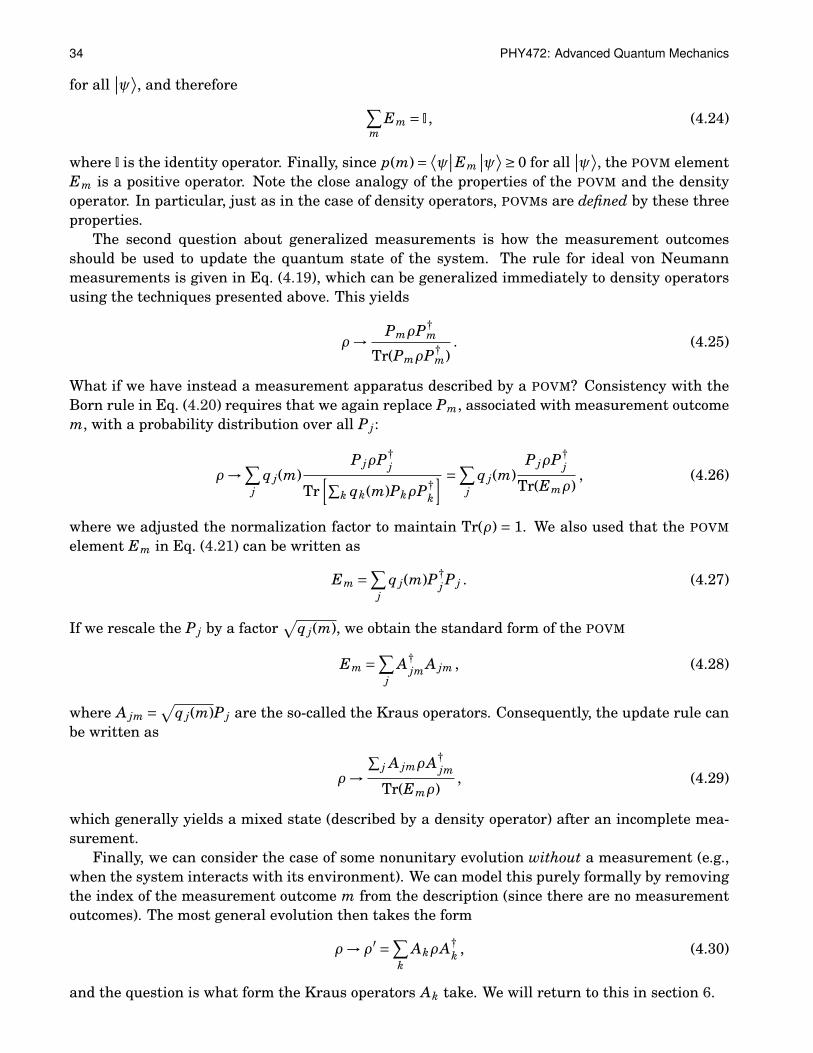
The second question about generalized measurements is how the measurement outcomesshould be used to update the quantum state of the system. The rule for ideal von Neumannmeasurements is given in Eq. (4.19), which can be generalized immediately to density operatorsusing the techniques presented above. This yields
ρ→ PmρP†m
Tr(PmρP†m)
. (4.25)
What if we have instead a measurement apparatus described by a POVM? Consistency with theBorn rule in Eq. (4.20) requires that we again replace Pm, associated with measurement outcomem, with a probability distribution over all P j:
ρ→∑
jq j(m)
P jρP†j
Tr[∑
k qk(m)PkρP†k
] =∑
jq j(m)
P jρP†j
Tr(Emρ), (4.26)
where we adjusted the normalization factor to maintain Tr(ρ) = 1. We also used that the POVM
element Em in Eq. (4.21) can be written as
Em =∑
jq j(m)P†
j P j . (4.27)
If we rescale the P j by a factor√
q j(m), we obtain the standard form of the POVM
Em =∑
jA†
jm A jm , (4.28)
where A jm =√q j(m)P j are the so-called the Kraus operators. Consequently, the update rule can
be written as
ρ→∑
j A jmρA†jm
Tr(Emρ), (4.29)
which generally yields a mixed state (described by a density operator) after an incomplete mea-surement.
Finally, we can consider the case of some nonunitary evolution without a measurement (e.g.,when the system interacts with its environment). We can model this purely formally by removingthe index of the measurement outcome m from the description (since there are no measurementoutcomes). The most general evolution then takes the form
ρ→ ρ′ =∑k
AkρA†k , (4.30)
and the question is what form the Kraus operators Ak take. We will return to this in section 6.
Section 4: Mixed States and the Density Operator 35
Exercises
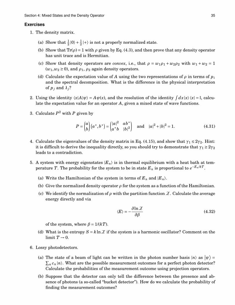
1. The density matrix.
(a) Show that 12 |0⟩+ 1
2 |+⟩ is not a properly normalized state.
(b) Show that Tr(ρ)= 1 with ρ given by Eq. (4.3), and then prove that any density operatorhas unit trace and is Hermitian.
(c) Show that density operators are convex, i.e., that ρ = w1ρ1 +w2ρ2 with w1 +w2 = 1(w1,w2 ≥ 0), and ρ1, ρ2 again density operators.
(d) Calculate the expectation value of A using the two representations of ρ in terms of piand the spectral decomposition. What is the difference in the physical interpretationof p j and λ j?
2. Using the identity ⟨x|A|ψ⟩ = Aψ(x), and the resolution of the identity∫
dx |x⟩⟨x| = I, calcu-late the expectation value for an operator A, given a mixed state of wave functions.
3. Calculate P2 with P given by
P =(ab
)(a∗,b∗)= (|a|2 ab∗
a∗b |b|2)
and |a|2 +|b|2 = 1. (4.31)
4. Calculate the eigenvalues of the density matrix in Eq. (4.15), and show that γ1 ≤ 2γ2. Hint:it is difficult to derive the inequality directly, so you should try to demonstrate that γ1 ≥ 2γ2leads to a contradiction.
5. A system with energy eigenstates |En⟩ is in thermal equilibrium with a heat bath at tem-perature T. The probability for the system to be in state En is proportional to e−En/kT .
(a) Write the Hamiltonian of the system in terms of En and |En⟩.(b) Give the normalized density operator ρ for the system as a function of the Hamiltonian.
(c) We identify the normalization of ρ with the partition function Z . Calculate the averageenergy directly and via
⟨E⟩ =−∂ lnZ
∂β(4.32)
of the system, where β= 1/(kT).
(d) What is the entropy S = k lnZ if the system is a harmonic oscillator? Comment on thelimit T → 0.
6. Lossy photodetectors.
(a) The state of a beam of light can be written in the photon number basis |n⟩ as∣∣ψ⟩ =∑
n cn |n⟩. What are the possible measurement outcomes for a perfect photon detector?Calculate the probabilities of the measurement outcome using projection operators.
(b) Suppose that the detector can only tell the difference between the presence and ab-sence of photons (a so-called “bucket detector”). How do we calculate the probability offinding the measurement outcomes?

36 PHY472: Advanced Quantum Mechanics
(c) Real bucket detectors have a finite efficiency η, which means that each photon has aprobability η of triggering the detector. Calculate the probabilities of the measurementoutcomes.
(d) What other possible imperfections do realistic bucket detectors have?
7. An electron with spin state∣∣ψ⟩ = α |↑⟩ +β |↓⟩ and |α|2 + |β|2 = 1 is sent through a Stern-
Gerlach apparatus to measure the spin in the z direction (i.e., the |↑⟩, |↓⟩ basis).
(a) What are the possible measurement outcomes? If the position of the electron is mea-sured by an induction loop rather than a screen, what is the state of the electron im-mediately after the measurement?
(b) Suppose that with probability p the induction loops fail to give a current signifying thepresence of an electron. What are the three possible measurement outcomes? Give thePOVM.
(c) Calculate the probabilities of the measurement outcomes, and the state of the electronimediately after the measurement (for all possible outcomes).
37
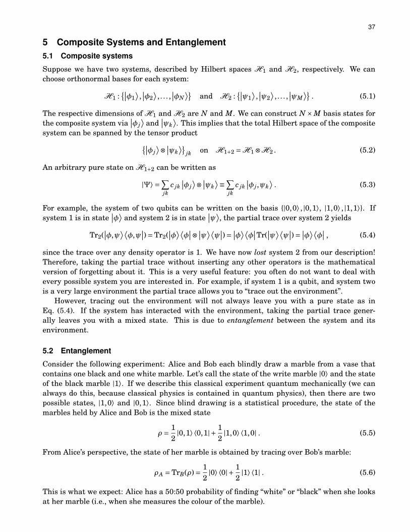
5 Composite Systems and Entanglement5.1 Composite systems
Suppose we have two systems, described by Hilbert spaces H1 and H2, respectively. We canchoose orthonormal bases for each system:
H1 :∣∣φ1
⟩,∣∣φ2
⟩, . . . ,
∣∣φN⟩
and H2 :∣∣ψ1
⟩,∣∣ψ2
⟩, . . . ,
∣∣ψM⟩
. (5.1)
The respective dimensions of H1 and H2 are N and M. We can construct N ×M basis states forthe composite system via
∣∣φ j⟩
and∣∣ψk
⟩. This implies that the total Hilbert space of the composite
system can be spanned by the tensor product∣∣φ j⟩⊗ ∣∣ψk
⟩jk on H1+2 =H1 ⊗H2 . (5.2)
An arbitrary pure state on H1+2 can be written as
|Ψ⟩ =∑jk
c jk∣∣φ j
⟩⊗ ∣∣ψk⟩≡∑
jkc jk
∣∣φ j,ψk⟩
. (5.3)
For example, the system of two qubits can be written on the basis |0,0⟩ , |0,1⟩, |1,0⟩ , |1,1⟩. Ifsystem 1 is in state
∣∣φ⟩and system 2 is in state
∣∣ψ⟩, the partial trace over system 2 yields
Tr2(∣∣φ,ψ
⟩⟨φ,ψ
∣∣)=Tr2(∣∣φ⟩⟨
φ∣∣⊗ ∣∣ψ⟩⟨
ψ∣∣)= ∣∣φ⟩⟨
φ∣∣Tr(
∣∣ψ⟩⟨ψ
∣∣)= ∣∣φ⟩⟨φ
∣∣ , (5.4)
since the trace over any density operator is 1. We have now lost system 2 from our description!Therefore, taking the partial trace without inserting any other operators is the mathematicalversion of forgetting about it. This is a very useful feature: you often do not want to deal withevery possible system you are interested in. For example, if system 1 is a qubit, and system twois a very large environment the partial trace allows you to “trace out the environment”.
However, tracing out the environment will not always leave you with a pure state as inEq. (5.4). If the system has interacted with the environment, taking the partial trace gener-ally leaves you with a mixed state. This is due to entanglement between the system and itsenvironment.
5.2 Entanglement
Consider the following experiment: Alice and Bob each blindly draw a marble from a vase thatcontains one black and one white marble. Let’s call the state of the write marble |0⟩ and the stateof the black marble |1⟩. If we describe this classical experiment quantum mechanically (we canalways do this, because classical physics is contained in quantum physics), then there are twopossible states, |1,0⟩ and |0,1⟩. Since blind drawing is a statistical procedure, the state of themarbles held by Alice and Bob is the mixed state
ρ = 12|0,1⟩⟨0,1|+ 1
2|1,0⟩⟨1,0| . (5.5)
From Alice’s perspective, the state of her marble is obtained by tracing over Bob’s marble:
ρA =TrB(ρ)= 12|0⟩⟨0|+ 1
2|1⟩⟨1| . (5.6)
This is what we expect: Alice has a 50:50 probability of finding “white” or “black” when she looksat her marble (i.e., when she measures the colour of the marble).

38 PHY472: Advanced Quantum Mechanics
Next, consider what the state of Bob’s marble is when Alice finds a white marble. Just fromthe setup we know that Bob’s marble must be black, because there was only one white and oneblack marble in the vase. Let’s see if we can reproduce this in our quantum mechanical descrip-tion. Finding a white marble can be described mathematically by a projection operator |0⟩⟨0| (seeEq. (2.24)). We need to include this operator in the trace over Alice’s marble’s Hilbert space:
ρB = TrA(|0⟩A ⟨0|ρ)Tr(|0⟩A ⟨0|ρ)
= |1⟩⟨1| , (5.7)
which we set out to prove: if Alice finds that when she sees that her marble is white, she de-scribes the state of Bob’s marble as black. Based on the setup of this experiment, Alice knowsinstantaneously what the state of Bob’s marble is as soon as she looks at her own marble. Thereis nothing spooky about this; it just shows that the marbles held by Alice and Bob are correlated.
Next, consider a second experiment: By some procedure, the details of which are not importantright now, Alice and Bob each hold a two-level system (a qubit) in the pure state
|Ψ⟩AB = |0,1⟩+ |1,0⟩p2
. (5.8)
Since |1,0⟩ and |0,1⟩ are valid quantum states, by virtue of the first postulate of quantum mechan-ics |Ψ⟩AB is also a valid quantum mechanical state. It is not difficult to see that these systems arealso correlated in the states |0⟩ and |1⟩: When Alice finds the value “0”, Bob must find the value“1”, and vice versa. We can write this state as a density operator
ρ = 12
(|0,1⟩+ |1,0⟩)(⟨0,1|+⟨1,0|)
= 12
(|0,1⟩⟨0,1|+ |0,1⟩⟨1,0|+ |1,0⟩⟨0,1|+ |1,0⟩⟨1,0|) . (5.9)
Notice the two extra terms with respect to Eq. (5.5). If Alice now traces out Bob’s system, shefinds that the state of her marble is
ρA =TrB(ρ)= 12|0⟩⟨0|+ 1
2|1⟩⟨1| . (5.10)
In other words, even though the total system was in a pure state, the subsystem held by Alice(and Bob, check this) is mixed! We can try to put the two states back together:
ρA ⊗ρB =(12|0⟩⟨0|+ 1
2|1⟩⟨1|
)⊗
(12|0⟩⟨0|+ 1
2|1⟩⟨1|
)= 1
4(|0,0⟩⟨0,0|+ |0,1⟩⟨0,1|+ |1,0⟩⟨1,0|+ |1,1⟩⟨1,1|) , (5.11)
but this is not the state we started out with! It is also a mixed state, instead of the pure state westarted with. Since mixed states mean incomplete knowledge, there must be some information inthe combined system that does not reside in the subsystems alone! This is called entanglement.
Entanglement arises because states like (|0,1⟩+|1,0⟩)/p
2 cannot be written as a tensor productof two pure states
∣∣ψ⟩⊗∣∣φ⟩. These latter states are called separable. In general a state is separable
if and only if it can be written as
ρ =∑
jp j ρ
(A)j ⊗ρ(B)
j . (5.12)

Section 5: Composite Systems and Entanglement 39
Classical correlations such as the black and white marbles above fall into the category of separa-ble states.
So far, we have considered the quantum states in the basis |0⟩ , |1⟩. However, we can alsodescribe the same system in the rotated basis |±⟩ according to
|0⟩ = |+⟩+ |−⟩p2
and |1⟩ = |+⟩− |−⟩p2
. (5.13)
The entangled state |Ψ⟩AB can then be written as
|0,1⟩+ |1,0⟩p2
= |+,+⟩−|−,−⟩p2
, (5.14)
which means that we have again perfect correlations between the two systems with respect to thestates |+⟩ and |−⟩. Let’s do the same for the state ρ in Eq. (5.5) for classically correlated marbles.After a bit of algebra, we find that
ρ =14
(|++⟩⟨++|+ |+−⟩⟨+−|+ |−+⟩⟨−+|+ |−−⟩⟨−−|−|++⟩⟨−−|− |−−⟩⟨++|− |+−⟩⟨−+|− |−+⟩⟨+−|) . (5.15)
Now there are no correlations in the conjugate basis |±⟩, which you can check by calculatingthe conditional probabilities of Bob’s state given Alice’s measurement outcomes. This is anotherkey difference between classically correlated states and entangled states. A good interpretationof entanglement is that entangled systems exhibit correlations that are stronger than classicalcorrelations. We will shortly see how these stronger correlations can be used in informationprocessing.
We have seen that operators, just like states, can be combined into tensor products:
A⊗B∣∣φ⟩⊗ ∣∣ψ⟩= A
∣∣φ⟩⊗B∣∣ψ⟩
. (5.16)
And just like states, some operators cannot be written as A⊗B:
C =∑k
Ak ⊗Bk . (5.17)
This is the most general expression of an operator in the Hilbert space H1⊗H2. In Dirac notationthis becomes
C =∑
jklmφ jklm
∣∣φ j⟩⟨φk
∣∣⊗ ∣∣φl⟩⟨φm
∣∣= ∑jklm
φ jklm∣∣φ j,φl
⟩⟨φk,φm
∣∣ . (5.18)
As an example, the Bell operator is diagonal on the Bell basis:∣∣Φ±⟩= |0,0⟩± |1,1⟩p2
and∣∣Ψ±⟩= |0,1⟩± |1,0⟩p
2. (5.19)
The eigenvalues of the Bell operator are not important, as long as they are not degenerate (why?).A measurement of the Bell operator projects onto an eigenstate of the operator, which is an entan-gled state. Consequently, we cannot implement such composite measurements by measuring eachsubsystem individually, because those individual measurements would project onto pure statesof the subsystems. And we have seen that the subsystems of pure entangled states are mixedstates.

40 PHY472: Advanced Quantum Mechanics
A particularly useful technique when dealing with two systems is the so-called Schmidt decom-position. In general, we can write any pure state over two systems as a superposition of basisstates:
|Ψ⟩ =dA∑j=1
dB∑k=1
c jk∣∣φ j
⟩A
∣∣ψk⟩
B , (5.20)
where dA and dB are the dimensions of the Hilbert spaces of system A and B, respectively, andwe order the systems such that dB ≥ dA. It turns out that we can always simplify this descriptionand write |Ψ⟩ as a single sum over basis states. We state it as a theorem:
Theorem: Let |Ψ⟩ be a pure state of two systems, A and B with Hilbert spaces HA and HB ofdimension dA and dB ≥ dA, respectively. There exist orthonormal basis vectors
∣∣a j⟩
A forsystem A and
∣∣b j⟩
B for system B such that
|Ψ⟩ =∑
jλ j
∣∣a j⟩
A
∣∣b j⟩
B , (5.21)
with real, positive Schmidt coefficients λ j, and∑
jλ2j = 1. This decomposition is unique, and
the sum runs at most to dA, the dimension of the smallest Hilbert space. Traditionally,we order the Schmidt coefficients in descending order: λ1 ≥ λ2 ≥ . . .. The total number ofnon-zero λi is the Schmidt number.
The proof can be found in many graduate texts on quantum mechanics and quantum informationtheory.
Given the Schmidt decomposition for a bi-partite system, we can immediately write down thereduced density matrices for the sub-systems:
ρA =TrB(|Ψ⟩⟨Ψ|)=∑
jλ2
j∣∣a j
⟩A
⟨a j
∣∣ , (5.22)
and
ρB =TrA(|Ψ⟩⟨Ψ|)=∑
jλ2
j∣∣b j
⟩B
⟨b j
∣∣ . (5.23)
The basis states∣∣a j
⟩A and
∣∣b j⟩
B may have completely different physical meanings; here we careonly that the states of the decomposition can be labelled with a single index, as opposed to twoindices.
Conversely, when we have a single system in a mixed state
ρ =∑
jp j
∣∣a j⟩⟨
a j∣∣ , (5.24)
we can always construct a pure state |Ψ⟩ that obeys (λ j =pp j)
|Ψ⟩ =∑
jλ j
∣∣a j,b j⟩
, (5.25)
By virtue of the Schmidt decomposition. The state |Ψ⟩ is called the purification of ρ. Since manytheorems are easier to prove for pure states than for mixed states, purifications can make ourwork load significantly lighter.

Section 5: Composite Systems and Entanglement 41
When there is more than one non-zero λ j in Eq. (5.25), the state |Ψ⟩ is clearly entangled: thereis no alternative choice of λ j due to the uniqueness of the Schmidt decomposition that would resultin λ′
1 = 1 and all others zero. Moreover, the more uniform the values of λ j, the more the state isentangled. One possible measure for the amount of entanglement in |Ψ⟩ is the Shannon entropyH
H =−∑
jλ2
j log2λ2j . (5.26)
This is identical to the von Neumann entropy S of the reduced density matrix ρ of |Ψ⟩ given inEq. (5.24):
S(ρ)=−Tr(ρ log2ρ) . (5.27)
Both entropies are measured in classical bits.How do we find the Schmidt decomposition? Consider the state |Ψ⟩ from Eq. (5.20). The (not
necessarily square) matrix C with elements c jk needs to be transformed into a single array ofnumbers λ j. This is achieved by applying the singular-value decomposition:
c jk =∑
iu jidiivik , (5.28)
where u ji and vik are elements of unitary matrices U and V , respectively, and dii is a diagonalmatrix with singular values λi. The vectors in the Schmidt decomposition become
|ai⟩ =∑
ju ji
∣∣φ j⟩
and |bi⟩ =∑k
vik∣∣ψk
⟩. (5.29)
This is probably a good time to remind ourselves about the singular-value decomposition. Allwe need to do is find U and V , the rest is just matrix multiplication. To find U , we diagonalizeCC† and find its eigenvectors. These form the columns of U . Similarly, we diagonalize C†C andarrange the eigenvectors in columns to find V . If C is an n×m matrix, U should be n×n and Vshould be m×m.
5.3 Quantum teleportation
Probably the most extraordinary use of the quantum correlations present in entanglement isquantum teleportation. Alice and Bob share two entangled qubits, labelled 2 (held by Alice) and3 (held by Bob), in the state (|0,0⟩23 +|1,1⟩23)/
p2. In addition, Alice holds a qubit in the state∣∣ψ⟩
1 =α |0⟩1 +β |1⟩1 . (5.30)
The object of quantum teleportation is to transfer the state of qubit 1 to qubit 3, without eitherAlice or Bob gaining any information about α or β. To make things extra hard, the three qubitsmust not change places (so Alice cannot take qubit 1 and bring it to Bob).
Classically, this is an impossible task: we cannot extract enough information about α and β
with a single measurement to reproduce∣∣ψ⟩
faithfully, otherwise we could violate the no-cloningtheorem. However, in quantum mechanics it can be done (without violating no-cloning). Writethe total state as ∣∣χ⟩= ∣∣ψ⟩
1
∣∣Φ+⟩23 =
1p2
(α |000⟩+α |011⟩+β |100⟩+β |111⟩) . (5.31)

42 PHY472: Advanced Quantum Mechanics
Alice now performs a Bell measurement on her two qubits (1 and 2), which project them onto oneof the Bell states
∣∣Φ±⟩12 or
∣∣Ψ±⟩12. We write |00⟩, |01⟩, |10⟩, and |11⟩ in the Bell basis:
|00⟩ =∣∣Φ+⟩+|Φ−⟩
p2
|01⟩ =∣∣Ψ+⟩+|Ψ−⟩
p2
|10⟩ =∣∣Ψ+⟩−|Ψ−⟩
p2
|11⟩ =∣∣Φ+⟩−|Φ−⟩
p2
. (5.32)
We can use these substitutions to write the state∣∣χ⟩
before the measurement as
∣∣χ⟩=12
[α
∣∣Φ+⟩12 |0⟩3 +α |Φ−⟩12 |0⟩3 +α
∣∣Ψ+⟩12 |1⟩3 +α |Ψ−⟩12 |1⟩3
+β∣∣Ψ+⟩
12 |0⟩3 −β |Ψ−⟩12 |0⟩3 +β∣∣Φ+⟩
12 |1⟩3 −β |Φ−⟩12 |1⟩3]
=12
[∣∣Φ+⟩(α |0⟩+β |1⟩)+|Φ−⟩ (α |0⟩−β |1⟩)
+∣∣Ψ+⟩
(β |0⟩+α |1⟩)+|Ψ−⟩ (β |0⟩−α |1⟩)] . (5.33)
Alice finds one of four possible outcomes:
Φ+ : Tr12(∣∣Φ+⟩⟨
Φ+∣∣ ∣∣χ⟩⟨χ∣∣) →
∣∣ψ⟩3 =α |0⟩+β |1⟩ ,
Φ− : Tr12(|Φ−⟩⟨Φ−|∣∣χ⟩⟨
χ∣∣) →
∣∣ψ⟩3 =α |0⟩−β |1⟩ ,
Ψ+ : Tr12(∣∣Ψ+⟩⟨
Ψ+∣∣ ∣∣χ⟩⟨χ∣∣) →
∣∣ψ⟩3 =α |1⟩+β |0⟩ ,
Ψ− : Tr12(|Ψ−⟩⟨Ψ−|∣∣χ⟩⟨
χ∣∣) →
∣∣ψ⟩3 =α |1⟩−β |0⟩ . (5.34)
From these outcomes, it is clear that the state held by Bob is different for the different measure-ment outcomes of Alice’s Bell measurement. Let this sink in for a moment: After setting up theentangled state between Alice and Bob, who may be literally light years apart, Bob has done ab-solutely nothing to his qubit, yet its state is different depending on Alice’s measurement outcome.This suggests that there is some instantaneous communication taking place, possibly violatingcausality!
In order to turn the state of Bob’s qubit into the original state, Alice needs to send the mea-surement outcome to Bob. This will take two classical bits, because there are four outcomes. Thecorrection operators that Bob need to apply are as follows:
Φ+ : I , Φ− : Z , Ψ+ : X , Ψ− : ZX . (5.35)
So in each case Bob needs to do something different to his qubit. To appreciate how remarkablethis protocol is, here are some of its relevant properties:
1. No matter is transported, only the state of the system;
2. neither Alice nor Bob learns anything about α or β;
3. any attempt to use quantum teleportation for signaling faster than light is futile!

Section 5: Composite Systems and Entanglement 43
Exercises
1. Derive Eq. (5.15), and show that ρB = I/2 when Alice’s qubit is projected onto |+⟩.
2. Quantum teleportation. Write the Bell states as∣∣ψnm⟩= (|0,0⊕n⟩+ (−1)m |1,1⊕n⟩) /
p2 ,
where ⊕ denotes addition modulo 2 and n,m = 0,1.
(a) Write∣∣ψnm
⟩in terms of
∣∣ψ00⟩
and the Pauli operators X and Z acting on the secondqubit.
(b) Using the shared Bell state∣∣ψnm
⟩between Alice and Bob, and the two-bit measure-
ment outcome ( j,k) for Alice’s Bell measurement, determine the correction operator forBob.
(c) We now generalize to N-dimensional systems. We define the N2 entangled states
∣∣ψnm⟩= 1p
N
N−1∑j=0
e2πi jn/N | j, j⊕m⟩ ,
where n⊕m = n+m mod N. Prove that this is an orthonormal basis.
(d) Give the teleportation protocol for the N-dimensional Hilbert space.
(e) What is Bob’s state before he learns Alice’s measurement outcome?
3. Imperfect measurements.
(a) A two-qubit system (held by Alice and Bob) is in the anti-symmetric Bell state |Ψ−⟩.Calculate the state of Bob’s qubit if Alice measures her qubit in the state |0⟩. Hint:write the measurement procedure as a partial trace over Alice’s qubit.
(b) Now Alice’s measurement is imperfect, and when her apparatus indicates “0”, therewas actually a small probability p that the qubit was projected onto the state |1⟩.What is Bob’s state?
(c) If Alice’s (imperfect) apparatus has only two measurement outcomes, what will Bob’sstate be if she finds outcome “1”?
44 PHY472: Advanced Quantum Mechanics
6 Evolution of Open Quantum SystemsWe have considered mixed states, where the experimenter has incomplete information about thestate preparation procedure, and we have also seen that mixing arises in a system when it isentangled with another system. The combined system can still be pure, but the subsystem hasbecome mixed. This phenomenon arises often when we want to describe systems that have someinteraction with their environment. The interaction creates entanglement, and the system takenby itself evolves from a pure state to a mixed state. Such a system is called “open”, since it canleak quantum information to the environment. The theory of open quantum systems revolvesaround the so-called Lindblad equation.
6.1 The Lindblad equation
Next, we will derive the Lindblad equation, which is the direct extension of the Heisenberg equa-tion for the density operator, i.e., the mixed state of a system. We have seen in Eq. (4.30) thatformally, we can write the evolution of a density operator as a mathematical map E , such thatthe density operator ρ transforms into
ρ→ ρ′ = E (ρ)≡∑k
AkρA†k , (6.1)
where the Ak are the Kraus operators. Requiring that ρ′ is again a density operator (Tr(ρ′) = 1)leads to the restriction
∑k A†
k Ak = I.We want to describe an infinitesimal evolution of ρ, in order to give the continuum evolution
later on. We therefore have that
ρ′ = ρ+δρ =∑k
AkρA†k . (6.2)
Since δρ is very small, one of the Kraus operators must be close to the identity. Without loss ofgenerality we choose this to be A0, and then we can write
A0 = I+ (L0 − iK)δt and Ak = Lkpδt , (6.3)
where we introduced the Hermitian operators L0 and K , and the remaining Lk are not necessarilyHermitian. We could have written A0 = I+L0δt and keep L0 general (non-Hermitian as well), butit will be useful later on to explicitly decompose it into Hermitian parts. We can now write
A0ρA†0 = ρ+
[(L0 − iK)ρ+ρ(L0 + iK)
]δt+O(δt2)
AkρA†k = LkρL†
kδt . (6.4)
We can substitute this into Eq. (6.2), to obtain up to first order in δt
δρ =[(
L0ρ+ρL0)− i(Kρ−ρK)+
∑k 6=0
LkρL†k
]δt . (6.5)
We now give the continuum evolution by dividing by δt and taking the limit δt → dt:
dρdt
=−i[K ,ρ]+ L0,ρ+∑k 6=0
LkρL†k , (6.6)
where A,B = AB+BA is the anti-commutator of A and B. We are almost there, but we mustdetermine what the different terms mean. Suppose we consider the free evolution of the system.
Section 6: Evolution of Open Quantum Systems 45
Eq. (6.6) must then reduce to the Heisenberg equation for the density operator ρ in Eq. (4.7), andwe see that all Lk including L0 are zero, and K is proportional to the Hamiltonian K = H/ħ. Againfrom the general property that Tr(ρ)= 1 we have
Tr(
dρdt
)= 0→ L0 =−1
2
∑k 6=0
L†kLk . (6.7)
This finally leads to the Lindblad equation
dρdt
= 1iħ [H,ρ]+ 1
2
∑k
(2LkρL†
k − L†kLk,ρ
). (6.8)
The operators Lk are chosen such that they model the relevant physical processes. This maysound vague, but in practice it will be quite clear. For example, modelling a transition |1⟩ → |0⟩without keeping track of where the energy is going or coming from will require a single Lindbladoperator
L = γ |0⟩⟨1| , (6.9)
where γ is a real parameter indicating the strength of the transition. This can model both decayand excitations.
6.2 Positive and completely positive maps
We considered the evolution of the density operator under a family of Kraus operators in Eq. (4.30):
ρ→ ρ′ = E (ρ)=∑k
AkρA†k , (6.10)
where∑
k A†k Ak = I (that is, E is trace-preserving). When E transforms any positive operator
into another positive operator, we call it a positive map. We may be tempted to conclude thatall positive maps correspond to physically allowed transformations. After all, it maps densityoperators to density operators. Unfortunately, Nature (or Mathematics?) is not that tidy.
Consider the transpose of the density operator ρ→ ρT , which acts according to
ρ =∑i jρ i j |i⟩⟨ j| → ρT =
∑i jρ ji |i⟩⟨ j| . (6.11)
You can verify immediately that the trace is preserved in this operation (check this!), and ρT isagain a positive operator since the eigenvalues are identical to those of ρ. For example, considerthe qubit state (|0⟩+ i |1⟩)/
p2. The density operator and its transpose are
ρ = 12
(1 −ii 1
)and ρT = 1
2
(1 i−i 1
). (6.12)
The transpose therefore corresponds to the state (|0⟩− i |1⟩)/p
2. Now consider that the qubit ispart of an entangled state (|00⟩+ |11⟩)/
p2. The density operator is given by
ρ = 12
(|00⟩⟨00|+ |00⟩⟨11|+ |11⟩⟨00|+ |11⟩⟨11|) , (6.13)
and the partial transpose on the first qubit is
ρT = 12
(|00⟩⟨00|+ |10⟩⟨01|+ |01⟩⟨10|+ |11⟩⟨11|) . (6.14)

46 PHY472: Advanced Quantum Mechanics
The eigenvalues of ρ are all positive, but ρT has a negative eigenvalue! So ρT cannot be a densityoperator. Consequently, it is not correct to say that positive maps correspond to physical processes.We need to put another restriction on maps.
From the example of the partial transpose, we can deduce that maps must not only be pos-itive for the system S that they act on, but also positive on larger systems that include S as asubsystem. When this is the case, we call the map completely positive. There is a very impor-tant theorem in mathematics, called Kraus’ Representation Theorem, which states that maps ofthe form in Eq. (6.10) with the restriction that
∑k A†
k Ak = I is a completely positive map, andmoreover, that any completely positive map can be expressed in this form.
Exercises
1. (a) Show that∑
k A†k Ak = I,
(b) prove that any non-Hermitian square matrix can be written as A+ iB, with A and BHermitian,
(c) prove that L0 =−12∑
k 6=0 L†kLk.
2. Consider a two-level system (|0⟩, |1⟩) that has a dephasing process, modelled by the Lindbladoperators L1 = γ |0⟩⟨1| and L2 = γ |1⟩⟨0|.
(a) write down the Lindblad equation (choose H = 0 for simplicity).
(b) Calculate the evolution of the pure states |0⟩ and |+⟩ at t = 0. Hint: write the densitymatrix in the Pauli matrix basis I, X ,Y , Z. What can you say about the equilibriumstate of the system?
(c) Calculate and plot the entropy S(ρ) of the state ρ(t) as a function of γ and t.
3. Calculate the eigenvalues of ρT in Eq. (6.14).

47
7 Orbital Angular Momentum and SpinAngular momentum plays an important role in quantum mechanics, not only as the orbital an-gular momentum of electrons orbiting the central potentials of nuclei, but also as the intrinsicmagnetic moment of particles, known as spin, and even as isospin in high-energy particle physics.
7.1 Orbital angular momentum
From classical physics we know that the orbital angular momentum of a particle is given by thecross product of its position and momentum
L= r×p or L i = εi jkr j pk , (7.1)
where we used Einstein’s summation convention for the indices. In quantum mechanics, wecan find the operator for orbital angular momentum by promoting the position and momentumobservables to operators. The resulting orbital angular momentum operator turns out to be rathercomplicated, due to a combination of the cross product and the fact that position and momentumdo not commute. As a result, the components of orbital momentum do not commute with eachother. When we use [r j, pk]= iħδ jk, the commutation relation for the components of L becomes
[L i,L j]= iħεi jkLk . (7.2)
A set of relations like this is called an algebra, and the algebra here is called closed since we cantake the commutator of any two elements L i and L j, and express it in terms of another elementLk. Another (simpler) closed algebra is [x, px]= iħI and [x, I]= [px, I]= 0.
Since the components of angular momentum do not commute, we cannot find simultaneouseigenstates for Lx, L y, and Lz. We will choose one of them, traditionally denoted by Lz, andconstruct its eigenstates. It turns out that there is another operator, a function of all L is, thatcommutes with any component L j, namely L2 = L2
x +L2y +L2
z. This operator is unique, in thatthere is no other operator that differs from L2 in a nontrivial way and still commutes with all L is.We can now construct simultaneous eigenvectors for Lz and L2.
Since we are looking for simultaneous eigenvectors for the square of the angular momen-tum and the z-component, we expect that the eigenvectors will be determined by two quantumnumbers, l, and m. First, and without any prior knowledge, we can formally write down theeigenvalue equation for Lz as
Lz |l,m⟩ = mħ|l,m⟩ , (7.3)
where m is some real number, and we included ħ to fit the dimensions of angular momentum.We will now proceed with the derivation of the eigenvalue equation for L2, and determine thepossible values for l and m.
From the definition of L2, we have L2 −L2z = L2
x +L2y, and
⟨l,m|L2 −L2z |l,m⟩ = ⟨l,m|L2
x +L2y |l,m⟩ ≥ 0 . (7.4)
The spectrum of Lz is therefore bounded by
l ≤ m ≤ l (7.5)
for some value of l. We derive the eigenvalues of L2 given these restrictions. First, we define theladder operators
L± = Lx ± iL y with L− = L†+ . (7.6)

48 PHY472: Advanced Quantum Mechanics
The commutation relations with Lz and L2 are
[Lz,L±]=±ħL± , [L+,L−]= 2ħLz , [L±,L2]= 0 . (7.7)
Next, we calculate Lz(L+ |l,m⟩):
Lz(L+ |l,m⟩)= (L+Lz + [Lz,L+]) |l,m⟩ = mħL+ |l,m⟩+ħL+ |l,m⟩= (m+1)ħL+ |l,m⟩ . (7.8)
Therefore L+ |l,m⟩ ∝ |l,m+1⟩. By similar reasoning we find that L− |l,m⟩ ∝ |l,m−1⟩. Since wealready determined that −l ≤ m ≤ l, we must also require that
L+ |l, l⟩ = 0 and L− |l,−l⟩ = 0 . (7.9)
Counting the states between −l and +l in steps of one, we find that there are 2l +1 differenteigenstates for Lz. Since 2l +1 is a positive integer, l must be a half-integer (l = 0, 1
2 ,1, 32 ,2, . . .).
Later we will restrict this further to l = 0,1,2, . . .The next step towards finding the eigenvalues of L2 is to calculate the following identity:
L−L+ = (Lx − iL y)(Lx + iL y)= L2x +L2
y + i[Lx,L y]=L2 −L2z −ħLz . (7.10)
We can then evaluate
L−L+ |l, l⟩ = 0 ⇒ (L2 −L2z −ħLz) |l, l⟩ =L2 |l, l⟩− (l2 + l)ħ2 |l, l⟩ = 0 . (7.11)
It is left as an exercise (see exercise 1b) to show that
L2 |l,m⟩ = l(l+1)ħ2 |l,m⟩ . (7.12)
We now have derived the eigenvalues for Lz and L2.One aspect of our algebraic treatment of angular momentum we still have to determine is the
matrix elements of the ladder operators. We again use the relation between L±, and Lz and L2:
⟨l,m|L−L+ |l,m⟩ =l∑
j=−l⟨l,m|L− |l, j⟩⟨l, j|L+ |l,m⟩ . (7.13)
Both sides can be rewritten as
⟨l,m|L2 −L2z −ħLz |l,m⟩ = ⟨l,m|L− |l,m+1⟩⟨l,m+1|L+ |l,m⟩ , (7.14)
where on the right-hand-side we used that only the m+1-term survives. This leads to
[l(l+1)−m(m+1)]ħ2 = |⟨l,m+1|L+ |l,m⟩ |2 . (7.15)
The ladder operators then act as
L+ |l,m⟩ = ħ√
l(l+1)−m(m+1) |l,m+1⟩ , (7.16)
and
L− |l,m⟩ = ħ√
l(l+1)−m(m−1) |l,m−1⟩ . (7.17)

Section 7: Orbital Angular Momentum and Spin 49
We have seen that the angular momentum L is quantized, and that this gives rise to a discretestate space parameterized by the quantum numbers l and m. However, we still have to restrictthe values of l further, as mentioned above. We cannot do this using only the algebraic approach(i.e., using the commutation relations for L i), and we have to consider the spatial properties ofangular momentum. To this end, we write L i as
L i =−iħεi jk
(x j
∂
∂xk
), (7.18)
which follows directly from the promotion of r and p in Eq. (7.1) to quantum mechanical operators.In spherical coordinates,
r =√
x2 + y2 + z2 , φ= arctan( y
x
), θ = arctan
(√x2 + y2
z
), (7.19)
the angular momentum operators can be written as
Lx =−iħ(−sinφ
∂
∂θ−cotθ cosφ
∂
∂φ
),
L y =−iħ(cosφ
∂
∂θ−cotθsinφ
∂
∂φ
),
Lz =−iħ ∂
∂φ,
L2 =−ħ2[
1sinθ
∂
∂θ
(sinθ
∂
∂θ
)+ 1
sin2θ
∂2
∂φ2
]. (7.20)
The eigenvalue equation for Lz then becomes
Lzψ(r,θ,φ)=−iħ ∂
∂φψ(r,θ,φ)= mħψ(r,θ,φ) (7.21)
We can solve this differential equation to find that
ψ(r,θ,φ)= ζ(r,θ) eimφ . (7.22)
A spatial rotation over 2π must return the wave function to its original value, because ψ(r,θ,φ)must have a unique value at each point in space. This leads to ψ(r,θ,φ+2π)=ψ(r,θ,φ) and
eim(φ+2π) = eimφ , or e2πim = 1 . (7.23)
This means that m is an integer, which in turn means that l must be an integer also.
7.2 Spin
For orbital angular momentum we found that 2l+1 must be an integer, and moreover the spatialproperties of the wave function force l to be an integer as well. However, we can also constructstates with half-integer l, but this must then be an internal degree of freedom. This is called spinangular momentum, or spin for short. We will show later in the course that the spin observableis interpreted as an intrinsic magnetic moment of a system.
To describe spin, we switch from L to S, which is no longer related to r and p. The commuta-tion relations between the components Si are the same as for L i,
[Si,S j]= iħεi jkSk , (7.24)

50 PHY472: Advanced Quantum Mechanics
so S and L obey the same algebra. The commutation relations between S and L, r, and p vanish:
[Si,L j]= [Si, r j]= [Si, p j]= 0 . (7.25)
Therefore, spin generates a whole new vector space, since it commutes with observables thatthemselves do not commute (like r j and p j), and it is independent of the spatial degrees of free-dom.
Since the commutation relations for S (its algebra) are the same as for L, we can immediatelycopy the algebraic structure of the eigenstates and eigenvalues:
Sz |s,ms⟩ = msħ|s,ms⟩ , with s = 0,12
,1,32
,2, . . .
S2 |s,ms⟩ = s(s+1)ħ2 |s,ms⟩ . (7.26)
When s = 12 , the system has two levels (a qubit) with spin eigenstates
∣∣12 , 1
2
⟩and
∣∣12 ,−1
2
⟩. We often
write ms = +12 =↑ (“up”) and ms = −1
2 =↓ (“down”), which finds its origin in the measurementoutcomes of electron spin in a Stern-Gerlach apparatus.
Now that we have introduced a whole new vector space related to spin, how do we write thewave function of a particle with spin? Without spin, the wave function is a normal single-valuedfunction ψ(r, t) = ⟨r|ψ(t)⟩ of space and time coordinates. Now we have to add the spin degree offreedom. For each spin (↑ or ↓ when s = 1
2 ), we have a wave function ψ↑(r, t) for the particle withspin up, and ψ↓(r, t) for the particle with spin down. We can write this as a vector:
ψ(r, t)=(ψ↑(r, t)ψ↓(r, t)
). (7.27)
The spin degree of freedom generates a vector space, after all. The vector ψ is called a spinor.Expectation values are evaluated in the usual way, but now we have to sum over the spin
degree of freedom, as well as integrate over space. For example, the probability of finding aparticle with spin up in a region Ω of space is given by
p(↑,Ω)=∑
ms=↑,↓
∫Ω
drδms,↑|ψms(r, t)|2 =∫Ω
dr |ψ↑(r, t)|2 , (7.28)
and the expectation value of finding a particle with any spin in a region Ω of space is given by
p(Ω)=∑
ms=↑,↓
∫Ω
dr |ψms(r, t)|2 . (7.29)
The normalization of the spinor is such that∑ms=↑,↓
∫V
dr |ψms(r, t)|2 = 1 , (7.30)
where V is the entire space available to the particle (this may be the entire universe, or thevolume of a box with impenetrable walls, etc.).
If spin is represented by (2s+1)-dimensional spinors (vectors), then spin transformations (op-erators) are represented by (2s+1)× (2s+1) matrices. In the two-dimensional case, we have byconstruction:
Sz |↑⟩ =ħ2
(10
)and Sz |↓⟩ =−ħ
2
(01
), (7.31)
Section 7: Orbital Angular Momentum and Spin 51
which means that the matrix representation of Sz is given by
Sz =ħ2
(1 00 −1
). (7.32)
Next, the ladder operators act according to
S+ |↑⟩ = 0 , S+ |↓⟩ = ħ|↑⟩ , S− |↑⟩ = ħ|↓⟩ , S− |↓⟩ = 0 , (7.33)
which leads to the matrix representation
S+ =ħ(0 10 0
)and S− =ħ
(0 01 0
). (7.34)
From S± = Sx ± iSy we can then deduce that
Sx =ħ2
(0 11 0
)and Sy =
ħ2
(0 −ii 0
). (7.35)
We often define Si ≡ 12ħσi, where σi are the so-called Pauli matrices. Previously, we have called
these matrices X , Y , and Z. The commutation relations of the Pauli matrices are
[σi,σ j]= 2iεi jkσk or[σi
2,σ j
2
]= iεi jk
σk
2. (7.36)
Other important properties of the Pauli matrices are
σi,σ j≡σiσ j +σ jσi = 2δi jI (anti-commutator). (7.37)
They are both Hermitian and unitary, and the square of the Pauli matrices is the identity: σ2i = I.
Moreover, they obey an “orthogonality” relation
12
Tr(σiσ j)= δi j . (7.38)
The proof of this statement is as follows:
σiσ j =σiσ j +σ jσi −σ jσi = σi,σ j−σ jσi = 2δi jI−σ jσi . (7.39)
Taking the trace then yields
Tr(2δi jI−σ jσi)=Tr(σiσ j)=Tr(σ jσi) , (7.40)
or (using Tr(I)= 2)
2Tr(σ jσi)= 4δi j , (7.41)
which proves Eq. (7.38). If we define σ0 ≡ I, we can extend this proof to the four-dimensional case
12
Tr(σµσν)= δµν , (7.42)
with µ,ν= 0,1,2,3.
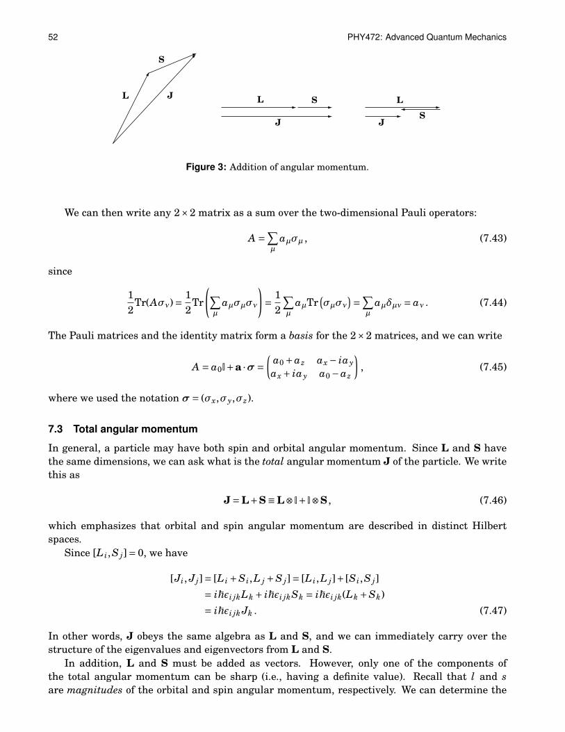
52 PHY472: Advanced Quantum Mechanics
L LL
S
S
S
J J
J
Figure 1: Addition of angular momentum.
1
Figure 3: Addition of angular momentum.
We can then write any 2×2 matrix as a sum over the two-dimensional Pauli operators:
A =∑µ
aµσµ , (7.43)
since
12
Tr(Aσν)= 12
Tr
(∑µ
aµσµσν
)= 1
2
∑µ
aµTr(σµσν
)=∑µ
aµδµν = aν . (7.44)
The Pauli matrices and the identity matrix form a basis for the 2×2 matrices, and we can write
A = a0I+a ·σ =(
a0 +az ax − iayax + iay a0 −az
), (7.45)
where we used the notation σ = (σx,σy,σz).
7.3 Total angular momentum
In general, a particle may have both spin and orbital angular momentum. Since L and S havethe same dimensions, we can ask what is the total angular momentum J of the particle. We writethis as
J=L+S≡L⊗ I+ I⊗S , (7.46)
which emphasizes that orbital and spin angular momentum are described in distinct Hilbertspaces.
Since [L i,S j]= 0, we have
[Ji, J j]= [L i +Si,L j +S j]= [L i,L j]+ [Si,S j]= iħεi jkLk + iħεi jkSk = iħεi jk(Lk +Sk)= iħεi jk Jk . (7.47)
In other words, J obeys the same algebra as L and S, and we can immediately carry over thestructure of the eigenvalues and eigenvectors from L and S.
In addition, L and S must be added as vectors. However, only one of the components ofthe total angular momentum can be sharp (i.e., having a definite value). Recall that l and sare magnitudes of the orbital and spin angular momentum, respectively. We can determine the

Section 7: Orbital Angular Momentum and Spin 53
extremal values of J, denoted by ± j, by adding and subtracting the spin from the orbital angularmomentum, as shown in Figure 3:
|l− s| ≤ j ≤ l+ s . (7.48)
For example, when l = 1 and s = 12 , the possible values of j are j = 1
2 and j = 32 .
The commuting operators for J are, first of all, J2 and Jz as we expect from the algebra, butalso the operators L2 and S2. You may think that Sz and Lz also commute with these operators,but that it not the case:
[J2,Lz]= [(L+S)2,Lz]= [L2 +2L ·S+S2,Lz]= 2[L,Lz] ·S 6= 0 . (7.49)
We can construct a full basis for total angular momentum in terms of J2 and Jz, as before:
J2 ∣∣ j,m j⟩=ħ2 j( j+1)
∣∣ j,m j⟩
and Jz∣∣ j,m j
⟩= m jħ∣∣ j,m j
⟩. (7.50)
Alternatively, we can construct spin and orbital angular momentum eigenstates directly as atensor product of the eigenstates
L2 |l,m⟩ |s,ms⟩ = ħ2l(l+1) |l,m⟩ |s,ms⟩ and Lz |l,m⟩ |s,ms⟩ = mħ|l,m⟩ |s,ms⟩ , (7.51)
and
S2 |l,m⟩ |s,ms⟩ = ħ2s(s+1) |l,m⟩ |s,ms⟩ and Sz |l,m⟩ |s,ms⟩ = msħ|l,m⟩ |s,ms⟩ . (7.52)
Since the Lz and Sz do not commute with J2, the states∣∣ j,m j
⟩are not the same as the states
|l,m⟩ |s,ms⟩.
7.4 Composite systems with angular momentum
Now consider two systems, 1 and 2, with total angular momentum J1 and J2, respectively. Thetotal angular momentum is again additive, and given by
J=J1 +J2 ≡J1 ⊗ I+ I⊗J2 . (7.53)
Completely analogous to the addition of spin and orbital angular momentum, we can constructthe commuting operators J2, Jz, J2
1, and J22, but not J1z and J2z. Again, we construct two natural
bases for the total angular momentum of the composite system, namely
| j,m⟩ or | j1,m1⟩⊗ | j2,m2⟩≡ | j1, j2,m1,m2⟩ . (7.54)
We want to know how the two bases relate to each other, because sometimes we wish to talkabout the angular momentum of the composite system, and at other times we are interestedin the angular momentum of the subsystems. Since the second basis (as well as the first) inEq. (7.54) forms a complete orthonormal basis, we can write
| j,m⟩ =∑
m1,m2
| j1, j2,m1,m2⟩⟨ j1, j2,m1,m2| j,m⟩ . (7.55)
The amplitudes ⟨ j1, j2,m1,m2| j,m⟩ are called Clebsch-Gordan coefficients, and we will now presenta general procedure for calculating them.

54 PHY472: Advanced Quantum Mechanics
Let’s first consider a simple example of two spin-12 systems, such as two electrons. The spin
basis for each electron is given by∣∣1
2 , 12
⟩= |↑⟩ and∣∣1
2 ,−12
⟩= |↓⟩. The spin basis for the two electronsis therefore
| j1, j2,m1,m2⟩ ∈ |↑,↑⟩ , |↑,↓⟩ , |↓,↑⟩ , |↓,↓⟩ . (7.56)
The total spin is given by j = 12 + 1
2 = 1 and j = 12 − 1
2 = 0, so the four basis states for total angularmomentum are
| j,m⟩ ∈ |1,1⟩ , |1,0⟩ , |1,−1⟩ , |0,0⟩ . (7.57)
The latter state is the eigenstate for j = 0. The maximum total angular momentum state |1,1⟩can occur only when the two electron spins a parallel, and we therefore have
|1,1⟩ = |↑,↑⟩ =∣∣1
2 , 12
⟩⊗ ∣∣12 , 1
2
⟩. (7.58)
To find the expansion of the other total angular momentum eigenstates in terms of spin eigen-states we employ the following trick: use that J± = J1±+ J2±. We can then apply J± to the state|1,1⟩, and J1±+ J2± to the state
∣∣12 , 1
2
⟩⊗ ∣∣12 , 1
2
⟩. This yields
J− |1,1⟩ = ħ√
j( j+1)−m(m−1) |1,0⟩ = ħp
2 |1,0⟩ . (7.59)
Similarly, we calculate
J1−∣∣1
2 , 12
⟩=ħ√
12 (3
2 )− 12 (−1
2 )∣∣1
2 ,−12
⟩=ħ∣∣1
2 ,−12
⟩, (7.60)
and a similar result for J2−. Therefore, we find that
ħp
2 |1,0⟩ = ħ|↑,↓⟩+ħ|↓,↑⟩ =⇒ |1,0⟩ = |↑,↓⟩+ |↓,↑⟩p2
. (7.61)
Applying J− again yields
|1,−1⟩ = |↓,↓⟩ . (7.62)
This agrees with the construction of adding parallel spins. The three total angular momentumstates
|1,1⟩ = |↑,↑⟩ ,
|1,0⟩ = 1p2
(|↑,↓⟩+ |↓,↑⟩) ,
|1,−1⟩ = |↓,↓⟩ (7.63)
form a so-called triplet of states with j = 1. We now have to find the final state corresponding toj = 0, m = 0. The easiest way to find it at this point is to require orthonormality of the four basisstates, and this gives us the singlet state
|0,0⟩ = 1p2
(|↑,↓⟩− |↓,↑⟩) . (7.64)
The singlet state has zero total angular momentum, and it is therefore invariant under rotations.
Section 7: Orbital Angular Momentum and Spin 55
In general, this procedure of finding the Clebsch-Gordan coefficients results in multiplets ofconstant j. In the case of two spins, we have a tensor product of two two-dimensional spaces,which are decomposed in two subspaces of dimension 3 (the triplet) and 1 (the singlet), respec-tively. We write this symbolically as
2⊗2= 3⊕1 . (7.65)
If we had combined a spin 1 particle with a spin 12 particle, the largest multiplet would have
been due to j = 1+ 12 = 3
2 , which is a 4-dimensional subspace, and the smallest subspace is due toj = 1− 1
2 = 12 , which is a two-dimensional subspace:
3⊗2= 4⊕2 . (7.66)
In general, the total angular momentum of two systems with angular momentum k and l isdecomposed into multiplets according to the following rule (k ≥ l):
(2k+1)⊗(2l+1)= [2(k+ l)+1]⊕ [2(k+ l)−1]⊕ . . .⊕ [2(k− l)+1] , (7.67)
or in terms of the dimensions of the subspaces (n ≥ m):
n⊗m= (n+m−1)⊕ (n+m−3)⊕ . . .⊕ (n−m+1) . (7.68)
Exercises
1. Angular momentum algebra.
(a) Prove the algebra given in Eq. (7.2). Also show that [L2,L i]= 0, and verify the commu-tation relations in Eq. (7.7).
(b) Show that L2 |l,m⟩ = l(l+1)ħ2 |l,m⟩. Use the fact that [L−,L2]= 0.
2. Pauli matrices.
(a) Check that the matrix representation of the spin-12 operators obey the commutation
relations.
(b) Calculate the matrix representation of the Pauli matrices for s = 1.
(c) Prove that exp[−iθ ·σ] is a 2×2 unitary matrix.
3. Isospin I describes certain particle families called multiplets, and the components of theisospin obey the commutation relations [I i, I j]= iεi jkIk.
(a) What is the relation between spin and isospin?
(b) Organize the nucleons (proton and neutron), the pions (π+, π0, and π−), and the deltabaryons (∆++, ∆+, ∆0, and ∆−) into multiplets. You will have to determine their isospinquantum number.
(c) Give all possible decay channels of the delta baryons into pions and nucleons (usecharge and baryon number conservation).
(d) Calculate the relative decay ratios of ∆+ and ∆0 into the different channels.
4. A simple atom has orbital and spin angular momentum, and the Hamiltonian for the atomcontains a spin-orbit coupling term Hso = għL ·S, where għ is the coupling strength.

56 PHY472: Advanced Quantum Mechanics
(a) Are orbital and spin angular momentum good quantum numbers for this system?What about total angular momentum?
(b) Use first-order perturbation theory to calculate the energy shift due to the spin-orbitcoupling term.
(c) Calculate the transition matrix elements of Hso in the basis|l,m; s,ms⟩.
5. Multiplets.
(a) A spin 32 particle and a spin 2 particle form a composite system. How many multiplets
are there, and what is the dimension of the largest multiplet?
(b) How many multiplets do two systems with equal angular momentum have?

57
8 Identical ParticlesWe have so far looked at the quantum mechanical description of a few particles with spin inthe previous section, and particles that exhibit entanglement in section 5. In all these cases,we assumed that the individual particles could be distinguished from each other. For example,the two-electron state (|↑↓⟩− |↓↑⟩)/
p2 assumes that we have two electrons, one held “over here”,
and the other “over there”, and we can talk meaningfully about their respective spins. The ten-sor product structure of our Hilbert space is a manifestation of our ability to label our particlesunambiguously.
However, what happens when we place the two electrons inside a sealed box? The wavefunctions of the electrons will quickly start to overlap. Since the electrons are identical particles,which according to basic quantum mechanics do not have well-defined paths, we cannot keeptrack of which electron is which inside the box. Not even in principle.
8.1 Symmetric and anti-symmetric states
The indistinguishability of identical particles means that we have to adjust our quantum me-chanical description of these objects. There are two ways of doing this, namely via a modificationof the allowed states and via a restructuring of the observables5. In this section we consider therestricted state space, and in the next we will be considering the new observables.
First of all, since the total number of particles is an observable quantity (for example bymeasuring the total charge in the box), we can give the particles an artificial labelling. The wavefunctions of the two particles are then given by
∣∣ψ(r1)⟩
1 for particle 1 at position r1, and∣∣φ(r2)
⟩2
for particle 2 at position r2. Since we can swap the positions of the particle without observableconsequences, we find that there are two states that denote the same physical situation:∣∣ψ(r1),φ(r2)
⟩12 and
∣∣ψ(r2),φ(r1)⟩
12 . (8.1)
However, we wish that each physically distinct situation has exactly one quantum state. Sincethere is no preference for either state, we can denote the physical situation of identical particlesat position r1 and r2 by the quantum state that is an equal weight over these two possibilities:
|Ψ(r1,r2)⟩12 =∣∣ψ(r1),φ(r2)
⟩12 + eiϕ ∣∣ψ(r2),φ(r1)
⟩12p
2. (8.2)
You can verify that swapping the positions r1 and r2 of the indistinguishable particles incurs onlya global (unobservable) phase. The question is now how we should choose φ.
Suppose that the two identical particles in the box are electrons. We know From Pauli’s ex-clusion principle that the two electrons cannot be in the same state. Therefore, when φ=ψ, thestate in Eq. (8.2) should naturally disappear:
|Ψ(r1,r2)⟩12 =∣∣ψ(r1),ψ(r2)
⟩12 + eiϕ ∣∣ψ(r2),ψ(r1)
⟩12p
2= 0 , (8.3)
which means that for particles obeying Pauli’s exclusion principle we must choose eiϕ =−1. Thequantum state of the two particles is anti-symmetric.
What about particles that do not obey Pauli’s exclusion principle? These must be restricted tostates that are orthogonal to the anti-symmetric states. In other words, they must be in states
5This is sometimes called second quantisation. This is a misnomer, since quantisation occurs only once, whenobservables are promoted to operators.

58 PHY472: Advanced Quantum Mechanics
that are symmetric under the exchange of two particles. For the two identical particles in a box,we therefore choose the value eiϕ =+1, which makes the state orthogonal to the anti-symmetricstate. The two possibilities for combining two identical particles are therefore
|ΨS(r1,r2)⟩ =∣∣ψ(r1),φ(r2)
⟩+ ∣∣ψ(r2),φ(r1)⟩
p2
,
|ΨA(r1,r2)⟩ =∣∣ψ(r1),φ(r2)
⟩− ∣∣ψ(r2),φ(r1)⟩
p2
. (8.4)
These states include both the internal degrees of freedom, such as spin, and the external degreesof freedom. So two electrons can still be in the state |↑↑⟩, as long as their spatial wave functionis anti-symmetric. The particles that are in a symmetric overall quantum state are bosons, whilethe particles in an overall anti-symmetric state are fermions.
We can extend this to N particles in a fairly straightforward manner. For bosons, we sum overall possible permutations of r1 to rN :
|ΨS(r1, . . . ,rN)⟩ = 1pN!
∑perm(r1,...,rN )
∣∣ψ1(r1), . . . ,ψN(rN)⟩
. (8.5)
For fermions, the odd permutations pick up a relative minus sign:
|ΨA(r1, . . . ,rN)⟩ = 1pN!
∑even
∣∣ψ1(r1), . . . ,ψN(rN)⟩− 1p
N!
∑odd
∣∣ψ1(r1), . . . ,ψN(rN)⟩
. (8.6)
This can be written compactly as the so-called Slater determinant
ΨA(r1, . . . ,rN)= 1pN!
∣∣∣∣∣∣∣∣∣ψ1(r1) ψ1(r2) . . . ψ1(rN)ψ2(r1) ψ2(r2) . . . ψ2(rN)
...... . . . ...
ψN(r1) ψN(r2) . . . ψN(rN)
∣∣∣∣∣∣∣∣∣ , (8.7)
where we removed the kets for notational convenience. The N particles in the state |ΨA(r1, . . . ,rN)⟩automatically obey the Pauli exclusion principle.
8.2 Creation and annihilation operators
The second, and particularly powerful way to implement the description of identical particlesis via creation and annihilation operators. To see how this description arises, consider somesingle-particle Hermitian operator A with eigenvalues a j. On physical grounds, and regardlessof distinguishability, we require that n j particles in the eigenstate
∣∣a j⟩
of A must have a totalphysical value n j ×a j for the observable A. We can repeat this for all eigenvalues a j, and obtaina potentially infinite set of basis vectors
|n1,n2,n3, . . .⟩ ,
for all integer values of n j, including zero. You should convince yourself that this exhausts all thepossible ways any number of particles can be distributed over the eigenvalues a j. The spectrumof A can be bounded or unbounded, and discrete or continuous. It may even be degenerate. Forsimplicity we consider here an unbounded, non-degenerate discrete spectrum.
A special state is given by
|∅⟩ = |0,0,0, . . .⟩ , (8.8)

Section 8: Identical Particles 59
which indicates the state of no particles, or the vacuum. The numbers n j are called the occupationnumber, and any physical state can be written as a superposition of these states:
|Ψ⟩ =∞∑
n1,n2,n3,...=0cn1,n2,n3,... |n1,n2,n3, . . .⟩ . (8.9)
The basis states |n1,n2,n3, . . .⟩ span a linear vector space called a Fock space F . It is the directsum of the Hilbert spaces for zero particles H0, one particle H1, two particles, etc.:
F =H0 ⊕H1 ⊕H2 ⊕H3 ⊕·· · (8.10)
Since |Ψ⟩ is now a superposition over different particle numbers, we require operators thatchange the particle number. These are the creation and annihilation operators, a† and a respec-tively. Up to a proportionality constant that we will determine later, the action of these operatorsis defined by
a†j
∣∣n1,n2, . . . ,n j, . . .⟩∝ ∣∣n1,n2, . . . ,n j +1, . . .
⟩,
a j∣∣n1,n2, . . . ,n j, . . .
⟩∝ ∣∣n1,n2, . . . ,n j −1, . . .⟩
. (8.11)
So the operator a†j creates a particle in a state with eigenvalue a j, and the operator a j removes
a particle in a state with eigenvalue a j. These operators are each others’ Hermitian adjoint,since removing a particle is the time reversal of adding a particle. Clearly, when an annihilationoperator attempts to remove particles that are not there, the result must be zero:
a j∣∣n1,n2, . . . ,n j = 0, . . .
⟩= 0 . (8.12)
The vacuum is then defined as the state that gives zero when acted on by any annihilation opera-tor: a j |∅⟩ = 0 for any j. Notice how we have so far sidestepped the problem of particle swapping;we exclusively used aspects of the total particle number.
What are the basic properties of these creation and annihilation operators? In particular, weare interested in their commutation relations. We will now derive these properties from what wehave determined so far. First, note that we can create two particles with eigenvalues ai and a jin the system in any order, and the only difference this can make is in the normalisation of thestate:
a†i a
†j |Ψ⟩ =λa†
j a†i |Ψ⟩ , (8.13)
where λ is some complex number. Since state |Ψ⟩ is certainly not zero, we require that
a†ka†
l −λa†l a
†k = 0 . (8.14)
Since k and l are just dummy variables, we equally have
a†l a
†k −λa†
ka†l = 0 . (8.15)
We now substitute Eq. (8.15) into Eq. (8.14) to eliminate a†l a
†k. This leads to
(1−λ2) a†ka†
l = 0 , (8.16)
and therefore
λ=±1 . (8.17)

60 PHY472: Advanced Quantum Mechanics
The relation between different creation operators can thus take two forms. They can obey acommutation relation when λ=+1:
a†l a
†k − a†
ka†l =
[a†
l , a†k
]= 0 , (8.18)
or they can obey an anti-commutation relation when λ=−1:
a†l a
†k + a†
ka†l =
a†
l , a†k
= 0 , (8.19)
While creating the particles in different temporal order is not the same as swapping two particles,it should not come as a surprise that there are two possible situations (the commutation relationand the anti-commutation relation). We encountered two possibilities in our previous approach aswell, where we found that many-particle states are either symmetric or anti-symmetric. In fact,creation operators that obey the commutation relation produce symmetric states, while creationoperators that obey the anti-commutation relation produce anti-symmetric states. We also seethat the creation operators described by the anti-commutation relations naturally obey Pauli’sexclusion principle. Suppose that we wish to create two identical particles in the same eigenstate∣∣a j
⟩. The anti-commutation relations say that a†
j, a†j= 0, so
a†2j = 0 . (8.20)
Any higher powers of a†j will also be zero, and we can create at most one particle in the state
∣∣a j⟩.
Taking the adjoint of the commutation relations for the creation operators gives us the corre-sponding relations for the annihilation operators
al ak − akal = [al , ak]= 0 , (8.21)
or
al ak + akal = al , ak= 0 . (8.22)
The remaining question is now what the (anti-) commutation relations are for products of creationand annihilation operators.
We proceed along similar lines as before. Consider the operators a j and a†k with j 6= k, and
apply them in different orders to a state |Ψ⟩.
ai a†j |Ψ⟩ =µ a†
j ai |Ψ⟩ . (8.23)
The same argumentation as before leads to µ=±1. For different j and k we therefore find[a j, a
†k
]= 0 or
a j, a
†k
= 0 . (8.24)
Now let’s consider the case j = k. For the special case where |Ψ⟩ = |∅⟩, we find(a j a
†k −µ a†
j ak
)|∅⟩ = a j a
†k |∅⟩ = δ jk |∅⟩ , (8.25)
based on the property that a j |∅⟩ = 0. When l = k,(aka†
k −µ a†kak
)|∅⟩ = |∅⟩ , (8.26)

Section 8: Identical Particles 61
we find for the two possible values of µ
aka†k − a†
kak = 1 or aka†k + a†
kak = 1 (8.27)
which is equivalent to [ak, a†
k
]= 1 or
ak, a†
k
= 1 . (8.28)
To summarise, we have two sets of algebras for the creation and annihilation operators. Thealgebra in terms of the commutation relations is given by
[ak, al]=[a†
k, a†l
]= 0 and
[ak, a†
l
]= δkl . (8.29)
This algebra describes particles that obey Bose-Einstein statistics, or bosons. The algebra interms of anti-commutation relations is given by
ak, al=a†
k, a†l
= 0 and
ak, a†
l
= δkl . (8.30)
This algebra describes particles that obey Fermi-Dirac statistics, or fermions.Finally, we have to determine the constant of proportionality for the creation and annihilation
operators. We have already required that a j a†k |∅⟩ = δ jk |∅⟩. To determine the rest, we consider
a new observable that gives us the total number of particles in the system. We denote this ob-servable by n, and we see that it must be additive over all particle numbers for the differenteigenvalues of A:
n =∑
jn j , (8.31)
where n j is the number of particles in the eigenstate∣∣a j
⟩. The total number of particles does
not change if we consider a different observable (although the distribution typically will), so thisrelation is also true when we count the particles in the states
∣∣b j⟩. Pretty much the only way we
can achieve this is to choose
n =∑
jn j =
∑j
a†j a j =
∑j
b†j b j . (8.32)
For the case of n j particles in state∣∣a j
⟩this gives
a†j a j
∣∣n j⟩= n j
∣∣n j⟩
, (8.33)
where we ignored the particles in other states |ak⟩ with k 6= j for brevity. For the Bose-Einsteincase this leads to the relations
a j∣∣n j
⟩=√n j
∣∣n j −1⟩
and a†j
∣∣n j⟩=√
n j +1∣∣n j +1
⟩. (8.34)
For Fermi-Dirac statistics, the action of the creation and annihilation operators on number statesbecomes
a j |0⟩ j = 0 and a†j |0⟩ j = e−iα |1⟩ j ,
a j |1⟩ j = eiα |0⟩ j and a†j |1⟩ j = 0 . (8.35)
The phase factor eiα can be chosen ±1.

62 PHY472: Advanced Quantum Mechanics
8.3 Observables based on creation and annihilation operators
So far, we have considered only the basis states of many particles for a single observable A.What about other observables, in particular those that do not commute with A? We can make asimilar construction. Suppose an observable B has eigenvalues b j. We can construct creation andannihilation operators b†
j and b j that act according to
b†j
∣∣m1,m2, . . . ,m j, . . .⟩=√
m j +1∣∣m1,m2, . . . ,m j +1, . . .
⟩,
b j∣∣m1,m2, . . . ,m j, . . .
⟩=√m j
∣∣m1,m2, . . . ,m j −1, . . .⟩
. (8.36)
where m j is the number of particles with value b j. Typically, the basis states of two observablesare related via a single unitary transformation
∣∣b j⟩ = U
∣∣a j⟩
for all j. How does this relate thecreation and annihilation operators?
To answer this, let’s look at the single particle states. We can write the single-particle eigen-states
∣∣a j⟩
and∣∣b j
⟩as ∣∣a j
⟩= a†j |∅⟩ and
∣∣b j⟩= b†
j |∅⟩ . (8.37)
We assume that U does not change the vacuum6, so U |∅⟩ = |∅⟩. This means that we can relatethe two eigenstates via∣∣b j
⟩=U∣∣a j
⟩=Ua†j |∅⟩ =Ua†
j
(U†U
)|∅⟩ =Ua†
jU† |∅⟩ = b†
j |∅⟩ , (8.38)
where we have strategically inserted the identity I=U†U . This leads to the operator transforma-tion
b†j =Ua†
jU† . (8.39)
The Hermitian adjoint is easily calculated as b j =UaU†. It is left as an exercise for you to provethat
b†j =
∑k
u jk a†k and b j =
∑k
u∗k j ak , (8.40)
where u jk = ⟨ak|b j⟩.How do we construct operators using the creation and annihilation operators? Suppose that
a one-particle observable H has eigenvalues E j and eigenstates | j⟩. This can be, for example theHamiltonian of the system, which ensures that the physical values of the particles (the eigenval-ues) are additive. The operator for many identical particles then becomes
H =∑
jE j n j =
∑j
E j a†j a j , (8.41)
which transforms according to Eq. (8.40). More generally, the operator may not be written in theeigenbasis |n1,n2, . . .⟩, in which case it has the form
H =∑i j
Hi j b†i b j , (8.42)
where Hi j are matrix elements. The creation and annihilation operators a†j and a j diagonalise H,
and are sometimes called normal modes. The reason for this is that the creation and annihilationoperators for bosons obey the same mathematical rules as the raising and lowering operators forthe harmonic oscillator. The index j then denotes different oscillators. A system of coupled oscil-lators can be decomposed into normal modes, which are themselves isolated harmonic oscillators.
6This is a natural assumption when we are confined to the single particle Hilbert space, but there are generalunitary transformations for which this does not hold, such as the transformation to an accelerated frame.

Section 8: Identical Particles 63
0E j
Xn j\
1E j
1Xn j\
Figure 4: Left: Bose-Einstein distribution for different temperatures (µ = 0). The lowerthe temperature, the more particles occupy the low energy states. Right: Fermi-Dirac dis-tribution for different temperatures and µ= 1. The fermions will not occupy energy stateswith numbers higher than 1, and therefore higher energies are necessarily populated.The energy values E j form a continuum on the horizontal axis.
8.4 Bose-Einstein and Fermi-Dirac statistics
Finally, in this section we will derive the Bose-Einstein and Fermi-Dirac statistics. In particular,we are interested in the thermal equilibrium for a large number of (non-interacting) identicalparticles with some energy spectrum E j, which my be continuous.
Since the number of particles is not fixed, we are dealing with the Grand Canonical Ensemble.Its partition function Ξ is given by
Ξ=Tr[eµβn−βH
], (8.43)
where H is the many-body Hamiltonian, β= 1/kBT and µ is the chemical potential. The averagenumber of particles with single particle energy E j is then given by
⟨n j⟩ =−1β
∂ lnΞ∂E j
. (8.44)
For the simple case where H = ∑j E j n j and the creation and annihilation operators obey the
commutator algebra, the exponent can be written as
exp
[β
∑j
(µ−E j) a†j a j
]=
⊗j
∞∑n j=0
eβ(µ−E j)n j∣∣n j
⟩⟨n j
∣∣ , (8.45)
and the trace becomes
Ξ=∏
j
11− eβ(µ−E j)
. (8.46)
The average photon number for energy E j is
⟨n j⟩ =−1β
∂ lnΞ∂E j
=− 1βΞ
∂Ξ
∂E j= 1
e−β(µ−E j) −1. (8.47)
This is the Bose-Einstein distribution for particles with energy E j. It is shown for increasing E jin Fig. 4 on the left.
64 PHY472: Advanced Quantum Mechanics
Alternatively, if the creation and annihilation operators obey the anti-commutation relations,the sum over n j in Eq. (8.45) runs not from 0 to ∞, but over 0 and 1. The partition function of thegrand canonical ensemble then becomes
Ξ=∏
j
[1+ eβ(µ−E j)
], (8.48)
and the average number of particles with energy E j becomes
⟨n j⟩ =− 1βΞ
∂Ξ
∂ħω j= 1
e−β(µ−E j) +1. (8.49)
This is the Fermi-Dirac statistics for these particles, and it is shown in Fig. 4 on the right. Thechemical potential is the highest occupied energy at zero temperature, and in solid state physicsthis is called the Fermi level. Note the sign difference in the denominator with respect to theBose-Einstein statistics.

Section 8: Identical Particles 65
Exercises
1. Calculate the Slater determinant for three electrons and show that no two electrons can bein the same state.
2. Particle statistics.
(a) What is the probability of finding n bosons with energy E j in a thermal state?
(b) What is the probability of finding n fermions with energy E j in a thermal state?
3. Consider a system of (non-interacting) identical bosons with a discrete energy spectrum anda ground state energy E0. Furthermore, the chemical potential starts out lower than theground state energy µ< E0.
(a) Calculate ⟨n0⟩ and increase the chemical potential to µ → E0 (e.g., by lowering thetemperature). What happens when µ passes E0?
(b) What is the behaviour of ⟨nthermal⟩ ≡∑∞
j=1 ⟨n j⟩ as µ → E0? Sketch both ⟨n0⟩ and⟨nthermal⟩ as a function of µ. What is the fraction of particles in the ground state atµ= E0?
(c) What physical process does this describe?
4. The process U = exp(r a†1a†
2 − r∗a1a2) with r ∈ C creates particles in two systems, 1 and 2,when applied to the vacuum state |Ψ⟩ =U |∅⟩.
(a) Show that the bosonic operators a†1a†
2 and a1a2 obey the algebra
[K−,K+]= 2K0 and [K0,K±]=±K± ,
with K+ = K†−.
(b) For operators obeying the algebra in (a) we can write
erK+−r∗K− = exp[
r|r| tanh |r|K+
]exp
[−2ln(cosh |r|)K0
]×exp
[− r∗
|r| tanh |r|K−
]. (8.50)
Calculate the state |Ψ⟩ of the two systems.
(c) The amount of entanglement between two systems can be measured by the entropyS(r) of the reduced density matrix ρ1 =Tr1[ρ] for one of the systems. Calculate S(r)=−Tr[ρ1 lnρ1].
(d) What is the probability of finding n particles in system 1?

66 PHY472: Advanced Quantum Mechanics
9 Many-Body Problems in Quantum MechanicsIn this final section we study a variety of problems in many-body quantum mechanics. First, weintroduce the Hartree-Fock method for taking into account the effect of electron-electron interac-tions in atoms. Next, we describe spin waves in magnetic materials using the Heisenberg model.Third, we describe the behaviour of an atom interacting with photons in a cavity, and introducethe Jaynes-Cummings Hamiltonian. And finally, we take a brief look at the basic ideas behindquantum field theory.
9.1 Interacting electrons in atomic shells
Previously, you have encountered the Schrödinger equation for a particle in a central potential,which can be interpreted as an electron bound to a proton in a hydrogen atom. We found that theenergy levels are quantised with quantum number n. In addition, the spin and orbital angularmomentum is quantised with quantum numbers ms, l, and m, respectively (we assume that s = 1
2since we are considering electrons). We can denote the set of quantum numbers n, ms, l, and mby greek indices α, β,. . . , and the wave-functions uα(r) then form a complete orthonormal basisfor the bound electron.
It is tempting to keep this complete orthonormal basis for other atoms as well, and assumethat the ground state of an N-electron atom is the tensor product of the N lowest energy eigen-states, appropriately anti-symmetrized via the Slater determinant. Indeed, the periodic table isbased on this assumption. However, this ignores the fact that the electrons interact with eachother, and the ground state of a many-electron atom is different. The Hartree-Fock method isdesigned to take this into account. It is a constrained variational approach, in which the trialstate that is optimised over is forced to be a Slater determinant in order to keep the correct par-ticle statistics. In this section we present the Hartree-Fock method, and arrive at the Hartree-Fock equations, which can be solved iteratively. We follow the derivation given by Bransden andJoachain (Physics of Atoms and Molecules, 1983 pp. 320-339).
First, we specify the Hamiltonian. Using the notation r i = |ri| for the distance of the ith
electron from the nucleus, and r i j = |ri −r j| for the distance between electrons i and j, we findthat
H = H1 +H2 =−N∑
i=1
( ħ2
2m∇2
i +Zr i
)+
N∑i< j=1
1r i j
, (9.1)
where we used units in which e/4πε0 = 1 and the Hamiltonian is divided into the single elec-tron Hamiltonian (H1) and the inter-electron Hamiltonian (H2). We choose as a normalised trialquantum state Ψ(r1, . . . ,rN) the Slater determinant
Ψ(r1, . . . ,rN)= 1pN!
∣∣∣∣∣∣∣∣∣uα(r1) uβ(r1) . . . uν(r1)uα(r2) uβ(r2) . . . uν(r2)
...... . . . ...
uα(rN) uβ(rN) . . . uν(rN)
∣∣∣∣∣∣∣∣∣ , (9.2)
and calculate the expectation value of the Hamiltonian H. This must be larger or equal to theground state E0
⟨Ψ|H|Ψ⟩ ≥ E0 , (9.3)
and varying the trial state then allows us to minimise the expectation value. This will get us closeto the ground state energy.

Section 9: Many-Body Problems in Quantum Mechanics 67
Since the Slater determinant is a rather large expression, it will save us quite a bit of writingif we introduce the anti-symmetrisation operator A , such that
Ψ(r1, . . . ,rN)=p
N! A uα(r1)uβ(r2) . . .uν(rN)≡p
N! AΦH , (9.4)
where ΦH(r1, . . . ,rN) is the Hartree wave function. The operator A can then be written as a sumover permutations P of the labels α, β, . . .ν:
A = 1N!
∑P
(−1)P P , (9.5)
and A is a projection operator: A 2 =A =A †. Both H1 and H2 commute with A .Next, we calculate the expectation values ⟨Ψ|H1|Ψ⟩ and ⟨Ψ|H2|Ψ⟩. Since [H1,A ] = 0, we can
write
⟨Ψ|H1|Ψ⟩ = N! ⟨ΦH|A H1A |ΦH⟩ = N! ⟨ΦH|H1A2|ΦH⟩ = N! ⟨ΦH|H1A |ΦH⟩ . (9.6)
A permutation of the labels α, β, . . .ν leads to an orthonormal state and H1 is a sum over one-electron Hamiltonians. We can therefore write this as
⟨Ψ|H1|Ψ⟩ = N! ⟨ΦH|H1A |ΦH⟩ =∑P
(−1)P⟨ΦH|H1 P|ΦH⟩ =N∑
i=1⟨ΦH|hi|ΦH⟩
=∑α
⟨uα(ri)|hi|uα(ri)⟩ ≡∑α
Iα (9.7)
where hi is the single electron Hamiltonian
hi =− ħ2
2m∇2
i −Zr i
. (9.8)
Next, we calculate the expectation value ⟨Ψ|H2|Ψ⟩ of the two-electron interaction Hamiltoni-ans. Using the same reasoning as in Eq. (9.6), we find that
⟨Ψ|H2|Ψ⟩ = N! ⟨ΦH|H2A |ΦH⟩ . (9.9)
Substituting the explicit form of A , we find
⟨Ψ|H2|Ψ⟩ =∑i< j
∑P
(−1)P⟨ΦH
∣∣∣∣ Pr i j
∣∣∣∣ΦH
⟩=
∑i< j
⟨ΦH
∣∣∣∣1−Pi j
r i j
∣∣∣∣ΦH
⟩, (9.10)
where Pi j is the exchange operator of electrons i and j. This expression allows us to write
⟨Ψ|H2|Ψ⟩ =12
∑α,β
[⟨uα(ri)uβ(r j)
∣∣∣∣ 1r i j
∣∣∣∣uα(ri)uβ(r j)⟩
−⟨
uα(ri)uβ(r j)∣∣∣∣ 1r i j
∣∣∣∣uβ(ri)uα(r j)⟩]
. (9.11)
Note the swap of α and β in the last ket. This expectation value consists of two terms, namely thedirect term
Jαβ ≡⟨
uα(ri)uβ(r j)∣∣∣∣ 1r i j
∣∣∣∣uα(ri)uβ(r j)⟩
, (9.12)

68 PHY472: Advanced Quantum Mechanics
and the exchange term
Kαβ ≡⟨
uα(ri)uβ(r j)∣∣∣∣ 1r i j
∣∣∣∣uβ(ri)uα(r j)⟩
. (9.13)
The total expectation value therefore becomes
⟨Ψ|H|Ψ⟩ =∑α
Iα+12
∑α,β
(Jαβ−Kαβ
). (9.14)
The matrix elements Jαβ and Kαβ are real and symmetric in α and β.The second step towards the Hartree-Fock method is to find the minimum of E ≡ ⟨Ψ|H|Ψ⟩
by varying the uα(ri). This means finding δE = 0. However, we must keep the functions uα(ri)orthonormal to each other, and this imposes N2 constraints. We can incorporate these constraintsin the variational procedure by including Lagrange multipliers εαβ, and the variational equationbecomes
δE−∑α,β
εαβ δ⟨uα(r)|uβ(r)⟩ = 0 . (9.15)
There is no explicit reference to electron positions ri in ⟨uα(r)|uβ(r)⟩ since we are only interestedin its orthonormality properties. The Lagrange multipliers εαβ form the elements of a Hermitianmatrix.
The variational approach ultimately leads to a set of N coupled equations:
Eα uα(ri)=hiuα(ri)+∑β
⟨uβ(r j)
∣∣ r−1i j
∣∣uβ(r j)⟩
uα(ri)
−∑β
⟨uβ(r j)
∣∣ r−1i j
∣∣uα(r j)⟩
uβ(ri) , (9.16)
which are known as the Hartree-Fock equations. These can be solved by iteration up to anydesired precision.
9.2 Spin waves in solids
Consider a system of spins with a nearest-neighbour interaction. For a uniform interaction in alldirections, this is described by the Hamiltonian
H =±J∑(i, j)
Si ·S j =±J∑(i, j)
Sz,iSz, j +12
(S+,iS−, j +S−,iS+, j
). (9.17)
where J > 0 is the coupling strength between the spins,∑
(i, j) is the sum over all neighbouringpairs, and S± = Sx ± iSy. The physics described by this Hamiltonian is known as the Heisenbergmodel. The sign of the coupling (here made explicit) determines whether the spins want to lignup in parallel (−J) or antiparallel (+J). The former situation describes ferromagnets, while thelater describes anti-ferromagnets. The spin operators for different sites (i 6= j) commute with eachother, while the spin operators at the same site (i = j) obey the spin algebra of Eq. (7.24).
Both systems have a well-defined ground state. For the ferromagnet this is the tensor productof the ground state of each individual spin. We are interested in the behaviour of the excitationswith respect to this ground state. Due to the large degeneracy in the system (all the spins areof the same species with the same coupling J) the excitations act as identical quasi-particles.Consequently we can describe them using creation and annihilation operators. It turns out that

Section 9: Many-Body Problems in Quantum Mechanics 69
they behave like bosons. You can think of an excitation as a higher spin value at some site thatpropagates to its neighbours due to the interaction. This is called a spin wave.
Suppose that the spins are aligned in the positive z-direction (so we consider −J), and Szhas the maximum eigenvalue s. When the spin is lowered by ħ, this creates an excitation in thesystem, because the spin is no longer lined up. So the z-component of the spin at site j is given by
Sz, j = s− a†j a j , (9.18)
where a†j a j is the operator for the number of excitations at site j. Since S± raise and lower
the eigenvalue of Sz, we expect that S+ ∝ a and S− ∝ a†. When we insist on the commutationrelation [S+,S−]= 2Sz, they become
S+, j =(2s− a†
j a j
) 12 a j and S−, j =
(2s− a†
j a j
) 12 a†
j . (9.19)
This is known as the Holstein-Primakoff transformation.For small numbers, the operators S± can be approximated as
S+, j 'p
2s a j and S−, j 'p
2s a†j . (9.20)
This allows us to write the Heisenberg Hamiltonian of Eq. (9.17) with −J to lowest order as
H =−J∑(i, j)
[s2 + s
(a†
i a j + ai a†j − a†
i ai − a†j a j
)]. (9.21)
For a simple cubic lattice of side L, lattice constant a and total number of spins N = (L/a)3 weexpect the spin waves to have wave vectors
k= 2πL
(m,n, o) with m,n, o ∈N , (9.22)
and 1≤ m,n, o ≤ L. The spin sites must now be indicated by a vector r instead of a single numberj, and the Fourier transformation of a†
r and ar is given by
ar =1pN
∑k
e−ik·r ak and a†r =
1pN
∑k
eik·r a†k , (9.23)
which transforms the Heisenberg Hamiltonian to
H =−3Js2N − JsN
∑r,d
∑k,k′
eir(k−k′)(eid·q−1
)a†
kak′
=−3Js2N − JsN
∑kε(k) a†
kak , (9.24)
where r is the position of a lattice site, d is the vector from a site to its nearest neighbours,which takes care of the sum over nearest neighbours. This is a diagonal Hamiltonian with eigen-energies
ε(k)= 2Js (3−coskxa−coskya−coskza) . (9.25)
This is the dispersion relation for the spin waves, and to lowest order (cos x ' 1 − 12 x2) it is
quadratic:
ε(k)= Jsa2k2 . (9.26)

70 PHY472: Advanced Quantum Mechanics
Spin waves are important when we want to manipulate magnetic properties with high frequency,such as in microwave devices. They carry energy, and are therefore a mechanism for dissipation.
For the case of anti-ferromagnets (+J), the ground state is harder to find. Consider an anti-ferromagnet that is again a simple cubic lattice with alternating spin ±s and lattice constant a.We can think of this lattice as two sub-lattices with constant spin, and redefine the spins on the−s sub-lattice according to
Sx →−Sx , Sy → Sy , and Sz →−Sz . (9.27)
These operators still obey the commutation relations of spin (which S →−S would not), and theHeisenberg Hamiltonian becomes
H =−J∑(i, j)
Sz,iSz, j +12
(S+,iS+, j +S−,iS−, j
). (9.28)
When we apply the Holstein-Primakoff transformation to this Hamiltonian, to first order weobtain
H =−J∑(i, j)
[s2 + s
(a†
i ai + b†j b j + ai b j + a†
i b†j
)], (9.29)
where a†i and ai are the creation and annihilation operators for the spin +s sub-lattice, and b†
jand b j are the creation and annihilation operators for the original spin −s sub-lattice. After theFourier transform of the creation and annihilation operators we get
H =−3Js2N +3Js∑k
[a†
kak+ b†−kb−k+ f (k)
(akb−k+ a†
kb†−k
)], (9.30)
where f (k)= 13 (coskxa+coskya+coskza).
To find the ground state we must diagonalise H so that it is a sum over number operators.This will involve mixing creation and annihilation operators. This is a unitary transformationthat can be written as
ak = uk ck−vk d†−k and b−k = uk d−k−vk c†
k . (9.31)
This leads to the Hamiltonian
H =−3Js(s+1)N +∑kε(k)
(c†
k ck+ d†−kd−k+1
), (9.32)
with the spin wave energy
ε(k)= 3Js(1− f (k)2) 1
2 . (9.33)
For small k the dispersion relation of the spin wave is linear in the wave vector, ε(k) 'p
3Jsa k,which means that the spin waves behave markedly different in ferromagnets and anti-ferromag-nets.

Section 9: Many-Body Problems in Quantum Mechanics 71
9.3 An atom in a cavity
Consider a two-level atom with bare energy eigenstates |g⟩ and |e⟩ and energy splitting ħω0. Thefree Hamiltonian H0 of the atom is given by
H0 =12ħω0
(1 00 −1
). (9.34)
The atom interacts with an electromagnetic wave, and the interaction is approximately the cou-pling between the dipole moment d associated with the |g⟩ ↔ |e⟩ transition and the electric fieldE, leading to the interaction Hamiltonian
Hint =−d ·E , (9.35)
where d = −er, and E is the classical, complex-valued electric field at the position of the atom.For an atom at the position r= 0, the electric field can be written as
E= E0ε eiωt +E0ε∗e−iωt , (9.36)
where E0 is the real amplitude of the electric field ε is the polarsation vector of the wave. Theoff-diagonal matrix elements of Hint are given by
⟨e|Hint|g⟩ = eE0⟨e|r|g⟩ ·ε eiωt +c.c., (9.37)
and c.c. denotes the complex conjugate. Since r has odd parity, the diagonal matrix elements⟨g|Hint|g⟩ and ⟨e|Hint|e⟩ vanish. When we define reg ≡ ⟨e|r|g⟩, the total Hamiltonian becomes
H =( 1
2ħω0 eE0r∗eg · (εeiωt +ε∗e−iωt)eE0reg · (εeiωt +ε∗e−iωt) −1
2ħω0
). (9.38)
Using the Rotating Wave Approximation (see exercise 9.1), this Hamiltonian can be written as
H = ħ2
(ν Ω∗
Ω −ν), (9.39)
where we made the substitution
ν=ω−ω0 and Ω= 2eE0
ħ reg ·ε . (9.40)
We can use the standard matrix techniques in quantum mechanics to solve for the eigenvalues,the eigenstates, and the time evolution of the atom.
Next, we consider the situation where atom is placed inside a cavity of volume V , and the elec-tric field in the cavity has angular frequency ω with wave vector k propagating in the z-direction.Assume that the length of the cavity is a multiple of λ/2, such that ω is a resonant cavity mode.The field is very weak, so that the classical description of E is no longer sufficient. In particular,the field is made of photons, i.e., identical bosons. Consequently, we need to express E in terms ofbosonic creation and annihilation operators a† and a, which create photons of frequency ω. Sincethe intensity of the field is proportional to both E 2
0 and a†a, we expect the electric field to be pro-portional to the creation and annihilation operators themselves. Hermiticity requires that it isproportional to the sum of the creation and annihilation operators. Furthermore, the electric fieldis a transverse standing wave cavity mode and must vanish at the mirrors due to the boundary

72 PHY472: Advanced Quantum Mechanics
conditions imposed by Maxwell’s equations. The spatial amplitude variation therefore includes afactor sinkz. For linear polarisation the operator form of E then becomes
E(z, t)= ε√
ħωε0V
(a e−iωt + a† eiωt
)sinkz , (9.41)
where we assumed that ε is real7. The creation and annihilation operators are thus the amplitudeoperators of the field. Note that by the analogy with the harmonic oscillator, the electric fieldoperator acts as a position operator of a particle in a harmonic potential well characterised by ω.
We again consider the dipole approximation of the atom in the field, and the Hamiltonian iswritten as
Hint =−d · E= e r ·ε√
ħωε0V
sinkz(a e−iωt + a† eiωt
). (9.42)
The operator r can be written as
r= reg |e⟩⟨g|+r∗eg |g⟩⟨e| , (9.43)
and for notational simplicity, we define the coupling constant g as
g = ereg ·ε√
ħωε0V
sinkz . (9.44)
We again calculate the matrix elements of Hint as before, but this time we write the operator interms of |g⟩⟨e| and |e⟩⟨g|:
Hint = g |e⟩⟨g|(a e−iωt + a† eiωt
)+ g∗ |g⟩⟨e|
(a e−iωt + a† eiωt
). (9.45)
It is convenient to express |g⟩⟨e| and |e⟩⟨g| in terms of the two-level raising and lowering opera-tors σ+ and σ−:
σ+ = |e⟩⟨g| and σ− = |g⟩⟨e| , (9.46)
with the commutation relation
[σ+,σ−]= 2σ3 with σ3 = |g⟩⟨g|− |e⟩⟨e| . (9.47)
The interaction Hamiltonian becomes
Hint = g σ+(a e−iωt + a† eiωt
)+ g∗ σ−
(a e−iωt + a† eiωt
). (9.48)
Including the free Hamiltonian for the field and the two-level atom, this becomes in the RotatingWave Approximation
HJC = 12ħω0 σ3 +ħω a†a+ g σ+ a + g∗σ− a† , (9.49)
This is the Jaynes-Cummings Hamiltonian for a two-level atom with energy splitting ħω0 inter-acting with a cavity mode of frequency ω. To achieve the strongest coupling g, the volume of thecavity should be small, and the atom should sit at an anti-node of the field.
7This is true for linear polarisation. For elliptical polarisation ε will be complex. The subsequent derivation willbe slightly modified (with more terms in Hint), but no extra technical or conceptual difficulties arise.

Section 9: Many-Body Problems in Quantum Mechanics 73
Quantities are conserved when they commute with the Hamiltonian. We can identify twoobservables that satisfy this requirement, namely the number of electrons
Pe = |g⟩⟨g|+ |e⟩⟨e| = I , (9.50)
and the total number of excitations
Ne = a†a+|e⟩⟨e| . (9.51)
This means that the Hamiltonian will not couple states with different total excitations.In a real system, the cavity will not be perfect, and the excited state of the atom will suffer
from spontaneous emission into modes other than the cavity mode. This can be modelled by aLindblad equation for the joint state ρ of the atom and the cavity mode. The Lindblad operatorfor a leaky cavity is proportional to the annihilation operator a, with a constant of proportionalitypκ that denotes the leakage rate. The spontaneous emission of the atom is modelled by the
Lindblad operator pγσ−. The Lindblad equation then becomes
dρdt
= 1iħ
[HJC,ρ
]+γσ−ρσ+−γ
2σ+σ−,ρ+κ aρa† − κ
2a†a,ρ . (9.52)
The research field of cavity quantum electrodynamics (or cavity QED) is devoted in a large partto solving this equation.
9.4 Outlook: quantum field theory
We have surreptitiously introduced the basic elements of non-relativistic quantum field the-ory. Consider again the Heisenberg model, where we described a lattice of spins with nearest-neighbour interactions. If we take the limit of the lattice constant a → 0 we end up with a contin-uum of creation and annihilation operators for each point in space. This is a field.
Traditionally we construct a quantum field theory from harmonic oscillators at each point inspace. To this end, we characterise a classical harmonic oscillator with mass M in terms of itsdisplacement q and velocity q. The equations of motion for the classical harmonic oscillator arethe Euler-Lagrange equations
ddt
∂L∂q
− ∂L∂q
= 0 , (9.53)
where L is the Lagrangian
L = 12
Mq2 − 12
K q2 , (9.54)
and K can be thought of as a spring constant. Substituting this L into Eq. (9.53) yields thefamiliar differential equations for the harmonic oscillator q+Ω2q = 0, with Ω2 = K /M.
Next, we arrange N particles in a one-dimensional lattice of length L and lattice constanta, where L = Na. Each particle’s displacement is coupled to the displacement of it’s nearestneighbours by a spring with constant K . The equations of motion of this set of coupled particlesis given by
qn =Ω2 [(qn+1 − qn)+ (qn−1 − qn)] . (9.55)

74 PHY472: Advanced Quantum Mechanics
We take the limit of a → 0 and N → ∞ while keeping L = Na fixed. Our variable qn(t) thenbecomes a field u(x, t), and it takes only a few lines of algebra to show that
u(x, t)= a2Ω2u′′(x, t)= v2u′′(x, t) with lima→0
aΩ= v . (9.56)
This is a wave equation, and v is the velocity of the wave. We can generalise this immediately tothree dimensions:
∂2u∂x2 + ∂2u
∂y2 + ∂2u∂z2 − 1
v2∂2u∂t2 = 0 . (9.57)
In quantum field theory, we consider only these waves as the field excitations, and ignore theunderlying particle structure we used to arrive at this result. We have already done somethingsimilar when we considered the spin waves in the Heisenberg model. Note also that the finitespeed of propagation of waves means that we can make the theory Lorentz invariant when v = c,the speed of light, and Eq. (9.57) becomes ∂µ∂µ u = 0.
The wave equation is typically derived from a Lagrangian L, or in the case of a field theory, theLagrangian density L . A massless scalar field is described by the Lorentz-invariant Lagrangiandensity
L = 12
[(∂φ
∂x
)2+
(∂φ
∂x
)2+
(∂φ
∂x
)2− 1
c2
(∂φ
∂x
)2]= 1
2(∂µφ)(∂µφ) , (9.58)
where for technical reasons we redefined φ = u/p
a. The dispersion relation for such a field isc2k2 =ω2, with k the wave number and ω the frequency of the wave. Similarly, a massive field isdescribed by
L = 12
(∂µφ)(∂µφ)− 12
m2φ2 . (9.59)
The Euler-Lagrange equation for this Lagrangian density is the so-called Klein-Gordon equation(∂µ∂
µ+ m2c2
ħ2
)φ= 0 . (9.60)
The mass term leads to a new dispersion relation
c2ħ2k2 −ħ2ω2 +m2c4 = 0 , (9.61)
and the group velocity for wave packets is
vg =dωdk
= c√1+µ2
with µ= mcħk
. (9.62)
For relativistic particles the momentum ħk is much larger than the rest mass mc, and thereforevg approaches c.
We can solve the Klein-Gordon equation formally by writing
φ(r, t)=∫
dk√2(2π)3ωk
(a(k) eik·r−iωt +a∗(k) e−ik·r+iωt
), (9.63)
where ak is the complex amplitude of a wave with wave vector k. The field is essentially asuperposition of (non-interacting) eigenmodes labelled by k, and we call this a free field. We can
Section 9: Many-Body Problems in Quantum Mechanics 75
introduce interactions between the waves in the field by adding higher-order terms to L withcoupling constants ν, λ,. . .
L = 12
(∂µφ)(∂µφ)− 12
m2φ2 − ν
3!φ3 − λ
4!φ4 −·· · (9.64)
The solution to the Klein-Gordon equation is now no longer the correct solution to the new equa-tions of motion, but when the interaction is reasonably weak we can use the solutions φ(r, t) ofthe free field as a starting point in a perturbation expansion.
So far, everything in this section has been a classical treatment. In order to extend the theory toquantum mechanics we have to quantise the field. We achieve this by promoting the amplitudesin φ (and therefore φ itself) to operators that obey commutation of anti-commutation relations
φ(r, t)=∫
dk√2(2π)3ωk
(a(k) eik·r−iωkt + a†(k) e−ik·r+iωkt
). (9.65)
These are the creation and annihilation operators for excitations of the field. For the Klein-Gordonequation they obey the bosonic commutation relations[
a(k), a(k′)]= [
a†(k), a†(k′)]= 0 and
[a(k), a†(k′)
]= δ3(k−k′) . (9.66)
The state of the field can then be written as a superposition of Fock states. The field φ has nowbecome an observable.
In quantum field theory, the excitations of the field are interpreted as particles. All funda-mental particles like quarks, electrons, photons, and the Higgs boson are excitations of a corre-sponding field. So the excitations of the Higgs field are Higgs bosons, and the excitations of theelectromagnetic field are photons. Spin-1
2 particles obey the Dirac equation(iħγµ∂µ−mc
)ψ= 0 , (9.67)
where the γµ are 4×4 matrices
γ0 =(I 00 −I
), γ1 =
(0 σx
−σx 0
), γ2 =
(0 σy
−σy 0
), γ3 =
(0 σz
−σz 0
), (9.68)
and ψ is a four-dimensional vector field called a spinor field. The solution to the free Dirac fieldcan be written as
ψ(r, t)=∑s
∫dk√
2(2π)3ωk
[bs(k) us(k) eik·r−iωkt + d†
s(k) vs(k) e−ik·r+iωkt]
, (9.69)
where s =±12ħ is the spin value, and us(k) and vs(k) are two spinors carrying the spin component
of the field
us(k)=N
(χs
ħcσ·kħω+mc2 χs
)and vs(k)=N
(− ħcσ·kħω+mc2 χsχs
), (9.70)
where N is a normalisation constant, σ is a vector of Pauli matrices, and
χ+ =(10
)and χ− =
(01
). (9.71)

76 PHY472: Advanced Quantum Mechanics
The creation and annihilation operators bs(k) and d†s(k) obey anti-commutation relations:
bs(k), br(k′)=
b†s(k), b†
r(k′)= 0 and
bs(k), b†
r(k′)= δrs δ
3(k−k′) ,ds(k), dr(k′)
= d†
s(k), d†r(k′)
= 0 and
ds(k), d†
r(k′)= δrs δ
3(k−k′) , (9.72)bs(k), dr(k′)
= b†
s(k), d†r(k′)
= 0 and
bs(k), d†
r(k′)=
ds(k), b†
r(k′)= 0 .
This means that the excitations of the Dirac field are fermions with spin 12 , such as the electron.
You see immediately that ψ is not Hermitian due to the appearance of d†. This means that ψis not an observable and we cannot think of the Dirac field as a quantised version of a classicalobservable field. There is no classical analog to the Dirac field. This is a consequence of the factthat the anti-particle of the Dirac excitations are not the same as the particle itself. E.g., thepositron is different from the electron. Anti-particles are a quintessentially quantum mechanicalphenomenon.
There is of course a lot more to quantum field theory than this. For example, the techniques fordoing the perturbation expansion of interacting fields leads to Feynman diagrams, and renormali-sation theory must be employed to deal with the infinities that crop up in the perturbation theory.Furthermore, one has to choose the right Lagrangian density, and principles such as gauge invari-ance and CPT invariance are imposed to constrain the possible choices. This leads ultimately tothe extraordinary successful Standard Model of particle physics. It the most fundamental theoryof Nature that we have, and it is tested to unprecedented accuracy.
Exercises
1. The Hamiltonian for a two-level atom in the presence of an electromagnetic wave, as givenin Eq. (9.38) depends on the time t. This makes it difficult to solve the Schrödinger equation,so in this exercise we will get rid of the time dependence by applying the Rotating WaveApproximation.
(a) If∣∣ψ′(t)
⟩ = U(t)∣∣ψ(t)
⟩, find the Schrödinger equation for
∣∣ψ′(t)⟩. What is the new
Hamiltonian?
(b) Choose U(t) such that
U(t)=(eiωt/2 0
0 e−iωt/2
),
and H is given by Eq. (9.38). Show that the new Hamiltonian is given by Eq. (9.39).
2. A two-level atom is placed in a perfect cavity with an electromagnetic field of frequency ω.
(a) Show that the Jaynes-Cummings Hamiltonian can be written as a direct sum of 2×2matrices Hn, and specify Hn.
(b) Diagonalize Hn to find the energy values of the system, and calculate the eigenstates.
(c) At t = 0, the system is in the state∣∣ψ(0)
⟩ = |e,n⟩. Calculate the state∣∣ψ(t)
⟩when the
light is on resonance with the atomic transition (ω=ω0).
(d) Calculate the amount of entanglement between the atom and the cavity field. Use therelative entropy as the entanglement measure.
(e) How long does the atom need to reside in the cavity in order to achieve maximumentanglement?