photovoltaic systems technology ss 2003
TRANSCRIPT
8/14/2019 Photovoltaic Systems Technology SS 2003
http://slidepdf.com/reader/full/photovoltaic-systems-technology-ss-2003 1/155
Photovoltaic Systems Technology
SS 2003
Universität Kassel
Rationelle Energiewandlung / Franz Kininger
Wilhelmshöher Alle 73
34121 Kassel
Germany
www.uni-kassel.de/re
8/14/2019 Photovoltaic Systems Technology SS 2003
http://slidepdf.com/reader/full/photovoltaic-systems-technology-ss-2003 2/155
-I-
t 0049- 561 804 6201i www.uni-kassel.de/re
Content
1 WORLD ENERGY SITUATION 1
1.1 Introduction 1 1.1 World Energy Consumption 1
1.2 Greenhouse Effect 4
1.3 Reserves and Resources 5
1.4 Regional Energy Consumption 10
1.5 Outlook for Energy Situation 13
1.6 References 14
2 SOLAR RADIATION 15
2.1 Introduction 15
2.2 Solar Radiation outside the Earth’s Atmosphere 17
2.3 Solar Radiation on the Earth’s Surface 18
2.4 Greenhouse Effect 24
2.5 Solar Radiation Measurement 27
2.6 References 30
3 FUNDAMENTALS OF PHOTOVOLTAICS 31
3.1 Introduction 31
3.2 Charge Transport in the Doped Silicon 32
3.3 Effects of a P-N Junction 33
3.4 Physical Processes in Solar Cells 35
3.4.1 Optical absorption 35
3.4.2 Recombination of charge carriers 35
3.4.3 Solar cells under incident light 36
3.5 Theoretical Description of the Solar Cell 37
3.6 Conditions with Real Solar Cells 41
3.6.1 Influence of series- and parallel resistance 41
3.6.2 Sources of losses in solar cells 43
3.7 Effect of Irradiation 44
3.8 Effect of Temperature 45
3.9 From Single Cells to PV Arrays 46
3.9.1 Parallel connection 46
3.9.2 Series connection 48
3.10 References 57
4 CONVERSION PRINCIPLES IN PV SYSTEMS 58
8/14/2019 Photovoltaic Systems Technology SS 2003
http://slidepdf.com/reader/full/photovoltaic-systems-technology-ss-2003 3/155
-II-
t 0049- 561 804 6201i www.uni-kassel.de/re
4.1 Introduction 58
4.2 Coupling of PV Generator and Ohmic Load 58
4.2.1 DC/DC converters 60
4.2.2 Maximum Power Point Tracker (MPPT) 68
4.3 Energy Storage Units 70
4.3.1 Electrochemical processes in the lead-acid batteries 71
4.3.2 Theoretical description of the lead-acid batteries 73
4.3.3 Gassing 76
4.3.4 The battery capacity 79
4.3.5 Requirements for the solar batteries 80
4.3.6 From single batteries to battery banks 83
4.4 Coupling of PV Generator and Battery 86 4.4.1 Self-regulating PV systems 88
4.5 Charge Regulators 89
4.5.1 Basic principles of charge regulators 89
4.5.2 Switching regulators 90
4.5.3 Control instruments 94
4.6 Inverters 94
4.6.1 General characteristics of PV inverters 94
4.6.2 Inverter principles 97
4.6.3 Power quality of inverters 105
4.6.4 Active quality control in the grid 108
4.6.5 Safety aspects with grid-connected inverters 109
4.7 References 111
5 PRINCIPLES OF PV SYSTEM CONFIGURATION 113
5.1 Introduction 113
5.2 Fundamental Structures of PV Systems 113
5.2.1 PV systems without battery storage 113
5.2.2 PV systems with battery storage 116
5.3 Future Trends of PV Systems 124
5.4 References 124
6 INTRODUCTION 125
6.1 Pre-sizing 125
6.2 Approximation of the System Cost 131
6.3 System Optimisation 132
6.3.1 Optimization process by hand 135
6.3.2 Optimization process by simulation programs 137
8/14/2019 Photovoltaic Systems Technology SS 2003
http://slidepdf.com/reader/full/photovoltaic-systems-technology-ss-2003 4/155
-III-
t 0049- 561 804 6201i www.uni-kassel.de/re
6.4 Sizing of System Components 138
6.5 References 142
7 ECONOMIC CALCULATION 143
7.1 Introduction 143
7.2 Annuity Method for Investment Decisions 143
7.3 Scenario Technique 144
7.4 Economic Calculation for the PV/Diesel Hybrid System 144
7.5 References 151

8/14/2019 Photovoltaic Systems Technology SS 2003
http://slidepdf.com/reader/full/photovoltaic-systems-technology-ss-2003 5/155
-1-t 0049- 561 804 6201i www.uni-kassel.de/re
1 World Energy Situation
1.1 Introduction
As 1973 the oil-exporting countries organized in the OPEC (Organization of the Petroleum
Exporting Countries) left the oil prices in the western world explode by supply boycotts, car-
free Sunday became reality in Germany. In addition, the national economies were pressed for
the energy shortage and high costs (Fig. 1-1). Then many people understood, how important
the supply security and how serious the consequence of a careless dependence on energy
resources and supplier countries can be. As a result the efficient use of energy ranks since
then quite above in the political priority.
Figure 1-1: Oil Crisis of 1973
Accordingly some experts feared 1973 and also later a lasting energy crisis because coal, oil
and gas are once only limited available. So far it has not come to the large scarceness - from
the reasons mentioned: first of all new fossil energy occurrences are discovered again and
again. Secondly there are in the meantime more efficient extraction techniques, so that the
exploitation of unprofitable sources is economically worthwhile. And thirdly industry and
citizens deal meanwhile substantially more economically with energy [7].
1.1 World Energy Consumption
However world energy consumption has still increased due to expected rapid increase of world
population (Fig. 1-2), especially in the third world and in new industrialized countries (NICs)
because ever more humans also need ever more energy. Continually rapid growth is foreseen in
the near future, with the world population rising from the present 6 billion to about 8 billion
over the next 25 years, and is expected to grow perhaps to 10 billion people by the middle of
21st century. Such a population increase will have a dramatic impact on energy demand, at least
doubling it by 2050, even if the developed countries adopt more effective energy conservation
policies so that their energy consumption does not increase at all over that period [1, 2, 3].

8/14/2019 Photovoltaic Systems Technology SS 2003
http://slidepdf.com/reader/full/photovoltaic-systems-technology-ss-2003 6/155
-2-t 0049- 561 804 6201i www.uni-kassel.de/re
Figure 1-2: World energy situation
(Source: Energy Information Administration 2001, International Energy Agency 2001, Scripps Institution of Oceanography 1999, Shell)
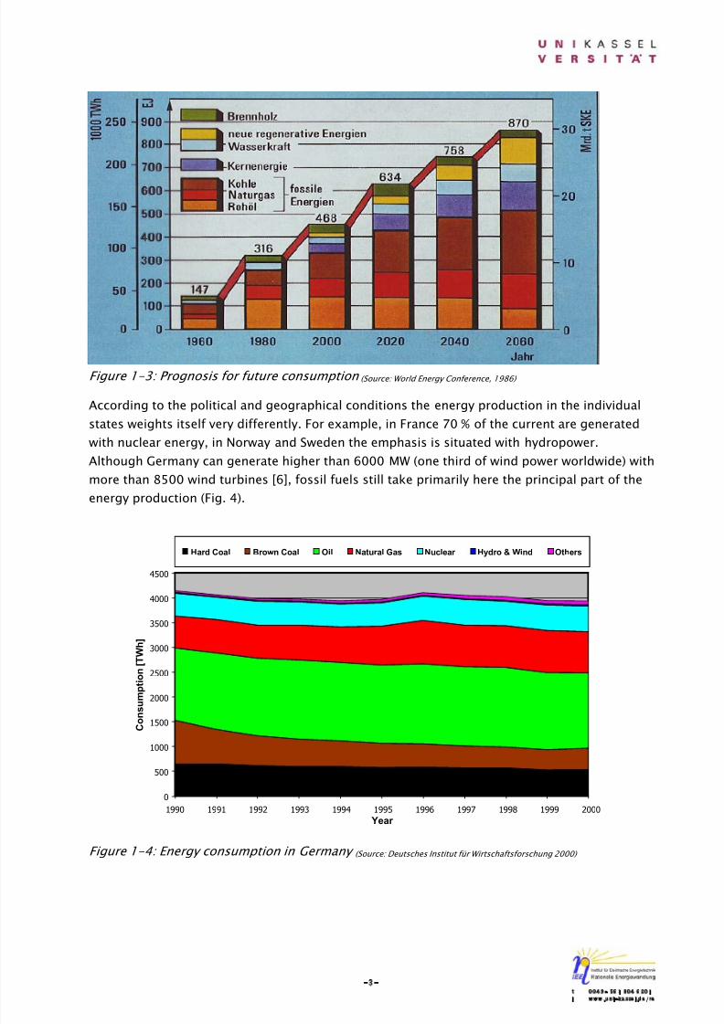
The world primary energy consumption 2000 approximately corresponds to a prediction of the
World Energy Conference 1986 in Cannes illustrated in Figure 1-3. Its further prognoses could
therefore point a global trend in the future. However most prognoses of the future energy
consumption were made before the Asian economic crisis. It was stated at the World Energy
Congress in Houston in September 1998 that the annual demand for primary energy would rise
to approx. 154 × 1012 kWh in the next 20 years. The World Energy Council expects that demand
will rise to 228 × 1012 kWh in 2050. Despite of increase in proportion of renewable energies it is
still expected that the role of fossil energy resources will not basically change in the near future
[5].
1930 1940 1950 1960 1970 1980 1990 2000
20
40
60
80
120
100
T o t a l & p e r c a p i t a e n e r g y c o n s u m p t i o n
0
4
8
12
16
20
W o r l d p o p u l a t i o n ,
C O 2 e m
i s s i o n
0
220
240
280
260
300
320
340
400
380
360
C O2 c on
c en t r a t i oni n t h e a t m o s ph er e
200
Year
World CO2 emission (Billion metric tons carbon equivalent)
World population growth (Billion)
Atmospheric CO2 concentration (ppm)
World energy consumption per capita (MWh)
World energy consumption (PWh)
Nuclear Hydro Other renewable energies
Coal Oil Gas
1900 1910 1920 1930 1940 1950 1960 1970 1980 1990 2000
20
40
60
80
120
100
T o t a l & p e r c a p i t a e n e r g y c o n s u m p t i o n
0
4
8
12
16
20
W o r l d p o p u l a t i o n ,
C O 2 e m
i s s i o n
0
220
240
280
260
300
320
340
400
380
360
C O2 c on
c en t r a t i oni n t h e a t m o s ph er e
200
Year
World CO2 emission (Billion metric tons carbon equivalent)
World population growth (Billion)
Atmospheric CO2 concentration (ppm)
World energy consumption per capita (MWh)
World energy consumption (PWh)
Nuclear Hydro Other renewable energies
Coal Oil Gas
1900 1910 1920
8/14/2019 Photovoltaic Systems Technology SS 2003
http://slidepdf.com/reader/full/photovoltaic-systems-technology-ss-2003 7/155
-3-t 0049- 561 804 6201i www.uni-kassel.de/re
Figure 1-3: Prognosis for future consumption (Source: World Energy Conference, 1986)
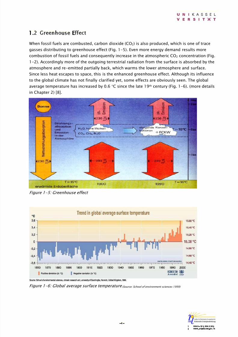
According to the political and geographical conditions the energy production in the individual
states weights itself very differently. For example, in France 70 % of the current are generated
with nuclear energy, in Norway and Sweden the emphasis is situated with hydropower.
Although Germany can generate higher than 6000 MW (one third of wind power worldwide) with
more than 8500 wind turbines [6], fossil fuels still take primarily here the principal part of the
energy production (Fig. 4).
0
500
1000
1500
2000
2500
3000
3500
4000
4500
1990 1991 1992 1993 1994 1995 1996 1997 1998 1999 2000
Year
C o n
s u m p t i o n [ T W h ]
Hard Coal Brown Coal Oil Natural Gas Nuclear Hydro & Wind Others
Figure 1-4: Energy consumption in Germany (Source: Deutsches Institut für Wirtschaftsforschung 2000)
8/14/2019 Photovoltaic Systems Technology SS 2003
http://slidepdf.com/reader/full/photovoltaic-systems-technology-ss-2003 8/155
-4-t 0049- 561 804 6201i www.uni-kassel.de/re
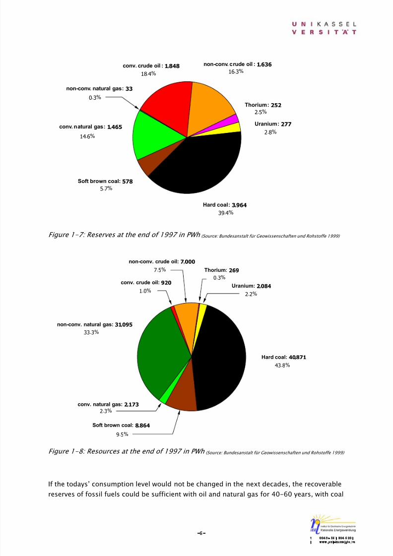
1.2 Greenhouse Effect
When fossil fuels are combusted, carbon dioxide (CO2) is also produced, which is one of trace
gasses distributing to greenhouse effect (Fig. 1-5). Even more energy demand results more
combustion of fossil fuels and consequently increase in the atmospheric CO2 concentration (Fig.
1-2). Accordingly more of the outgoing terrestrial radiation from the surface is absorbed by the
atmosphere and re-emitted partially back, which warms the lower atmosphere and surface.
Since less heat escapes to space, this is the enhanced greenhouse effect. Although its influence
to the global climate has not finally clarified yet, some effects are obviously seen. The global
average temperature has increased by 0.6 °C since the late 19th century (Fig. 1-6). (more details
in Chapter 2) [8].
Figure 1-5: Greenhouse effect
Figure 1-6: Global average surface temperature (Source: School of environment sciences 1999)

8/14/2019 Photovoltaic Systems Technology SS 2003
http://slidepdf.com/reader/full/photovoltaic-systems-technology-ss-2003 9/155
-5-t 0049- 561 804 6201i www.uni-kassel.de/re
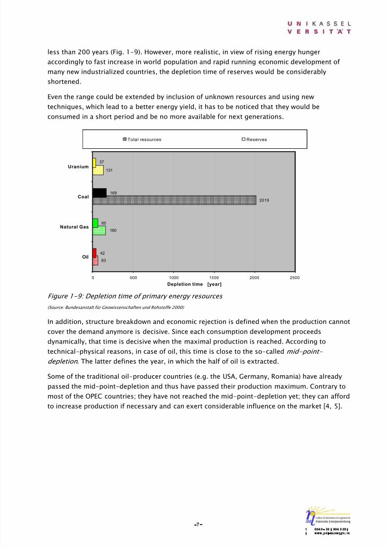
1.3 Reserves and Resources
Since primary energy consumption is dominated worldwide by fossil energy resources such as
crude oil, coal and natural gas, the increase in energy consumption has certainly direct effect to
reserves of them; they are going to be exhausted someday. Therefore the insight to the
restriction of reserves has also to be taken into account.
In order to avoid misunderstandings, the terms “reserves” and “resources” are defined here.
Reserves: that part of the total resources, which are documented in detail and can be recovered
economically by using current technology.
Resources: that part of the total resources, which are proved but at present not economically
recoverable, geologically indicated, or which for some other reasons cannot be assigned to the
reserves.
Total resources: reserves plus resources. It is to be noted that the reserves are not included inthe resources.
Regarding the definition, reserves are the quantity that can be recovered economically with the
available technology. This means that the quantity of reserves is a function of price. The
dependence of the amount of reserves on the price becomes especially clear in the case of
uranium, the only fuel whose reserves and resources have been rated for a long time according
to production costs ($130/kg U in 1993 and up to $80/kg U in 1997).
The increase in reserves and resources of conventional or non-conventional hydrocarbons are
not attributed to new discoveries but to re-evaluation of known fields (changes in the
evaluation criteria) and improved production methods.
According to Figure 1-7 and 1-8 coal is still dominant with the largest quantities of reserves
and resources worldwide. Coal reserves account for about 45 % of all energy resources.
Conventional and non-conventional crude oil, the second most important energy resources,
account for about 33 % (18.5 % and 16.3 %, respectively) of the reserves of all energy resources.
Natural gas follows in third place with approx. 15 %. Nuclear fuels account for approx. 5 %.
Although Thorium is not used for power generation as there are no operating thorium reactors,
the reserves of more that 2 million t Th can be considered as a basis for the future.
Energy resources are not evenly distributed in the world. The order of the countries rich in
energy resources is largely determined by coal reserves. For this reason, the USA is the country
with the largest energy reserves. China has the third larges energy reserves owing to its large
estimated coal reserves, and Russia has the second largest due to its large natural gas reserves.
Coal is also the reason why Australia is fourth in the list and India sixth. The most important oil
country, namely Saudi Arabia, occupies fifth place. Germany’s coal reserves are responsible for
its ninth place [4, 5].
8/14/2019 Photovoltaic Systems Technology SS 2003
http://slidepdf.com/reader/full/photovoltaic-systems-technology-ss-2003 10/155
-6-t 0049- 561 804 6201i www.uni-kassel.de/re
2.8%
39.4%
5.7%
14.6%
0.3%
2.5%
16.3%18.4%
conv. crude oil : 1,848 non-conv. crude oil : 1,636
conv. natural gas : 1,465
non-conv. natural gas : 33
Hard coal : 3,964
Soft brown coal: 578
Uranium : 277
Thorium : 252
Figure 1-7: Reserves at the end of 1997 in PWh (Source: Bundesanstalt für Geowissenschaften und Rohstoffe 1999)
43.8%
2.2%
7.5%
1.0%
2.3%
33.3%
0.3%
9.5%
conv. crude oil: 920
non-conv. crude oil: 7,000
conv. natural gas: 2,173
non-conv. natural gas: 31,095
Hard coal: 40,871
Soft brown coal: 8,864
Uranium: 2,084
Thorium: 269
Figure 1-8: Resources at the end of 1997 in PWh (Source: Bundesanstalt für Geowissenschaften und Rohstoffe 1999)
If the todays’ consumption level would not be changed in the next decades, the recoverablereserves of fossil fuels could be sufficient with oil and natural gas for 40-60 years, with coal
8/14/2019 Photovoltaic Systems Technology SS 2003
http://slidepdf.com/reader/full/photovoltaic-systems-technology-ss-2003 11/155
-7-t 0049- 561 804 6201i www.uni-kassel.de/re
less than 200 years (Fig. 1-9). However, more realistic, in view of rising energy hunger
accordingly to fast increase in world population and rapid running economic development of
many new industrialized countries, the depletion time of reserves would be considerably
shortened.
Even the range could be extended by inclusion of unknown resources and using newtechniques, which lead to a better energy yield, it has to be noticed that they would be
consumed in a short period and be no more available for next generations.
Figure 1-9: Depletion time of primary energy resources
(Source: Bundesanstalt für Geowissenschaften und Rohstoffe 2000)
In addition, structure breakdown and economic rejection is defined when the production cannot
cover the demand anymore is decisive. Since each consumption development proceeds
dynamically, that time is decisive when the maximal production is reached. According to
technical-physical reasons, in case of oil, this time is close to the so-called mid-point-
depletion . The latter defines the year, in which the half of oil is extracted.
Some of the traditional oil-producer countries (e.g. the USA, Germany, Romania) have already
passed the mid-point-depletion and thus have passed their production maximum. Contrary to
most of the OPEC countries; they have not reached the mid-point-depletion yet; they can afford
to increase production if necessary and can exert considerable influence on the market [4, 5].
131
2019
160
63
37
169
65
42
0 500 1000 1500 2000 2500
Oil
Natural Gas
Coal
Uranium
Depletion time [year]
Total resources Reserves
8/14/2019 Photovoltaic Systems Technology SS 2003
http://slidepdf.com/reader/full/photovoltaic-systems-technology-ss-2003 12/155
-8-t 0049- 561 804 6201i www.uni-kassel.de/re
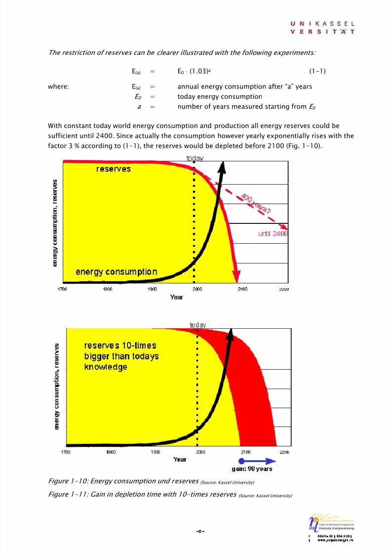
The restriction of reserves can be clearer illustrated with the following experiments:
E(a) = E0 ⋅ (1.03)a (1-1)
where: E(a) = annual energy consumption after “a” years
E 0 = today energy consumptiona = number of years measured starting from E 0
With constant today world energy consumption and production all energy reserves could be
sufficient until 2400. Since actually the consumption however yearly exponentially rises with the
factor 3 % according to (1-1), the reserves would be depleted before 2100 (Fig. 1-10).
Figure 1-10: Energy consumption und reserves (Source: Kassel University)
Figure 1-11: Gain in depletion time with 10-times reserves (Source: Kassel University)
8/14/2019 Photovoltaic Systems Technology SS 2003
http://slidepdf.com/reader/full/photovoltaic-systems-technology-ss-2003 13/155
-9-t 0049- 561 804 6201i www.uni-kassel.de/re
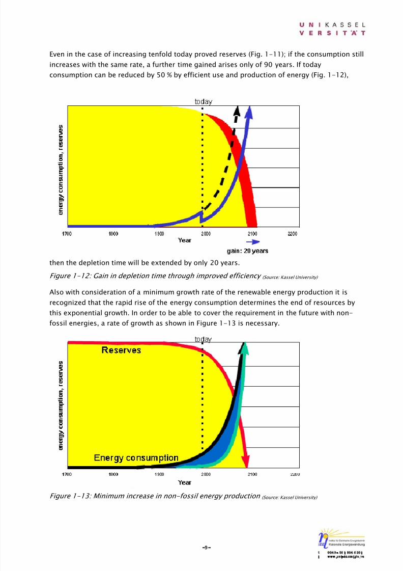
Even in the case of increasing tenfold today proved reserves (Fig. 1-11); if the consumption still
increases with the same rate, a further time gained arises only of 90 years. If today
consumption can be reduced by 50 % by efficient use and production of energy (Fig. 1-12),
then the depletion time will be extended by only 20 years.
Figure 1-12: Gain in depletion time through improved efficiency (Source: Kassel University)
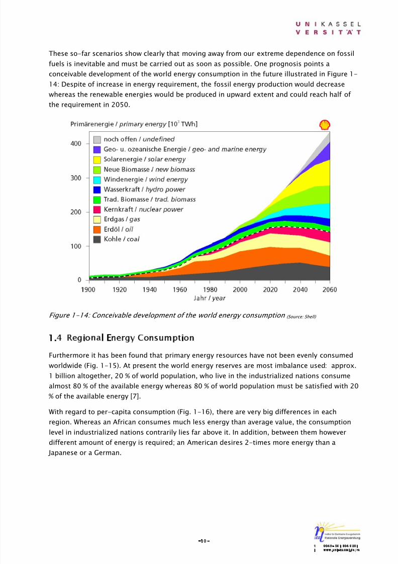
Also with consideration of a minimum growth rate of the renewable energy production it is
recognized that the rapid rise of the energy consumption determines the end of resources by
this exponential growth. In order to be able to cover the requirement in the future with non-
fossil energies, a rate of growth as shown in Figure 1-13 is necessary.
Figure 1-13: Minimum increase in non-fossil energy production (Source: Kassel University)
8/14/2019 Photovoltaic Systems Technology SS 2003
http://slidepdf.com/reader/full/photovoltaic-systems-technology-ss-2003 14/155
-10-t 0049- 561 804 6201i www.uni-kassel.de/re
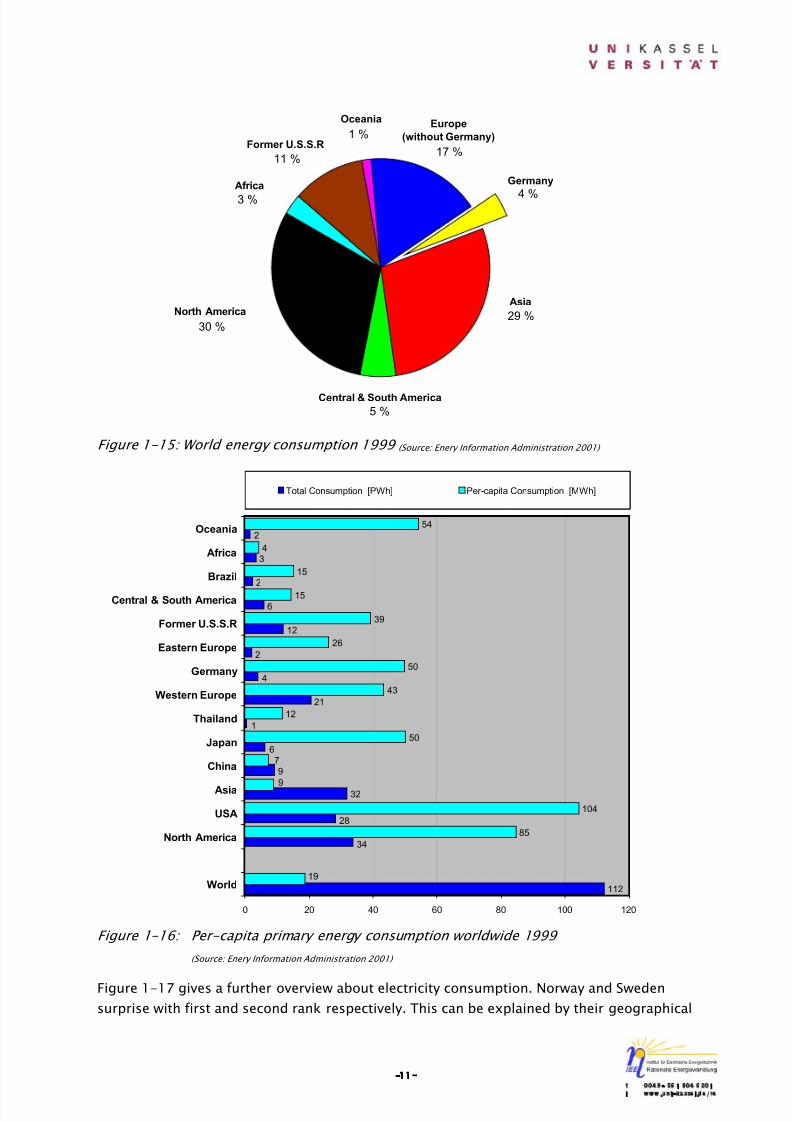
These so-far scenarios show clearly that moving away from our extreme dependence on fossil
fuels is inevitable and must be carried out as soon as possible. One prognosis points a
conceivable development of the world energy consumption in the future illustrated in Figure 1-
14: Despite of increase in energy requirement, the fossil energy production would decrease
whereas the renewable energies would be produced in upward extent and could reach half of
the requirement in 2050.
Figure 1-14: Conceivable development of the world energy consumption (Source: Shell)
1.4 Regional Energy Consumption
Furthermore it has been found that primary energy resources have not been evenly consumed
worldwide (Fig. 1-15). At present the world energy reserves are most imbalance used: approx.
1 billion altogether, 20 % of world population, who live in the industrialized nations consume
almost 80 % of the available energy whereas 80 % of world population must be satisfied with 20
% of the available energy [7].
With regard to per-capita consumption (Fig. 1-16), there are very big differences in each
region. Whereas an African consumes much less energy than average value, the consumption
level in industrialized nations contrarily lies far above it. In addition, between them however
different amount of energy is required; an American desires 2-times more energy than a
Japanese or a German.
8/14/2019 Photovoltaic Systems Technology SS 2003
http://slidepdf.com/reader/full/photovoltaic-systems-technology-ss-2003 15/155
-11-t 0049- 561 804 6201i www.uni-kassel.de/re
Figure 1-15: World energy consumption 1999 (Source: Enery Information Administration 2001)
Figure 1-16: Per-capita primary energy consumption worldwide 1999
(Source: Enery Information Administration 2001)
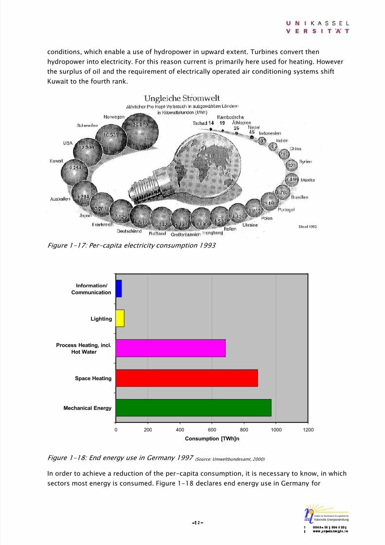
Figure 1-17 gives a further overview about electricity consumption. Norway and Sweden
surprise with first and second rank respectively. This can be explained by their geographical
112
32
85
104
50
12
43
50
26
39
15
15
4
54
2
3
2
6
12
2
4
21
1
6
9
28
34
7
9
19
0 20 40 60 80 100 120
World
North America
USA
Asia
China
Japan
Thailand
Western Europe
Germany
Eastern Europe
Former U.S.S.R
Central & South America
Brazil
Africa
Oceania
Total Consumption [PWh] Per-capita Consumption [MWh]
1 %
11 %
3 %
5 %
30 %29 %
17 %
4 %
Europe
(without Germany)
Germany
North America
Oceania
Former U.S.S.R
Africa
Central & South America
Asia
8/14/2019 Photovoltaic Systems Technology SS 2003
http://slidepdf.com/reader/full/photovoltaic-systems-technology-ss-2003 16/155
-12-t 0049- 561 804 6201i www.uni-kassel.de/re
conditions, which enable a use of hydropower in upward extent. Turbines convert then
hydropower into electricity. For this reason current is primarily here used for heating. However
the surplus of oil and the requirement of electrically operated air conditioning systems shift
Kuwait to the fourth rank.
Figure 1-17: Per-capita electricity consumption 1993
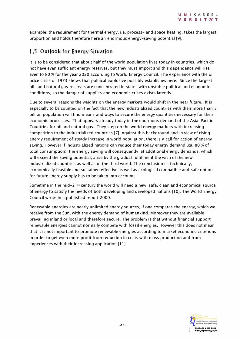
Figure 1-18: End energy use in Germany 1997 (Source: Umweltbundesamt, 2000)
In order to achieve a reduction of the per-capita consumption, it is necessary to know, in which
sectors most energy is consumed. Figure 1-18 declares end energy use in Germany for
0 200 400 600 800 1000 1200
Mechanical Energy
Space Heating
Process Heating, incl.
Hot Water
Lighting
Information/Communication
Consumption [TWh]n
8/14/2019 Photovoltaic Systems Technology SS 2003
http://slidepdf.com/reader/full/photovoltaic-systems-technology-ss-2003 17/155
-13-t 0049- 561 804 6201i www.uni-kassel.de/re
example: the requirement for thermal energy, i.e. process- and space heating, takes the largest
proportion and holds therefore here an enormous energy-saving potential [9].
1.5 Outlook for Energy Situation
It is to be considered that about half of the world population lives today in countries, which do
not have even sufficient energy reserves, but they must import and this dependence will rise
even to 80 % for the year 2020 according to World Energy Council. The experience with the oil
price crisis of 1973 shows that political explosive possibly establishes here. Since the largest
oil- and natural gas reserves are concentrated in states with unstable political and economic
conditions, so the danger of supplies and economic crises exists latently.
Due to several reasons the weights on the energy markets would shift in the near future. It is
especially to be counted on the fact that the new industrialized countries with their more than 3
billion population will find means and ways to secure the energy quantities necessary for their
economic processes. That appears already today in the enormous demand of the Asia-Pacific
Countries for oil and natural gas. They step on the world energy markets with increasing
competition to the industrialized countries [7]. Against this background and in view of rising
energy requirement of steady increase in world population, there is a call for action of energy
saving. However if industrialized nations can reduce their today energy demand (ca. 80 % of
total consumption), the energy saving will consequently let additional energy demands, which
will exceed the saving potential, arise by the gradual fulfillment the wish of the new
industrialized countries as well as of the third world. The conclusion is: technically,
economically feasible and sustained effective as well as ecological compatible and safe option
for future energy supply has to be taken into account.
Sometime in the mid-21st century the world will need a new, safe, clean and economical source
of energy to satisfy the needs of both developing and developed nations [10]. The World Energy
Council wrote in a published report 2000:
Renewable energies are nearly unlimited energy sources, if one compares the energy, which we
receive from the Sun, with the energy demand of humankind. Moreover they are available
prevailing inland or local and therefore secure. The problem is that without financial support
renewable energies cannot normally compete with fossil energies. However this does not mean
that it is not important to promote renewable energies according to market economic criterions
in order to get even more profit from reduction in costs with mass production and fromexperiences with their increasing application [11].
8/14/2019 Photovoltaic Systems Technology SS 2003
http://slidepdf.com/reader/full/photovoltaic-systems-technology-ss-2003 18/155
-14-t 0049- 561 804 6201i www.uni-kassel.de/re
1.6 References
[1] Energy Information Administration: Annual Energy Outlook 2001; Washington,
December 2000.
[2] Energy Information Administration: International Energy Outlook 2001; Washington,
March 2001.
[3] International Energy Agency: World Energy Outlook 2000 ; Paris, 2001.
[4] Federal Ministry of Economics and Technology: Energie Daten 2000: Nationale und
internationale Entwicklung , July 2000.
[5] Federal Institute for Geosciences and Natural Resources on behalf of the Federal
Ministry of Economics and Technology: Reserves, Resources and Availability of Energy Resources 1998 ; Hannover, 1999.
[6] Institut für Solare Energieversorgungstechnik: Windenergie Report Deutschland
1999/2000 ; Kassel, 2000.
[7] Institut der deutschen Wirtschaft Köln: Wirtschaft und Untericht: Informationen für
Pädagogen in Schule und Betrieb ; Köln, 2000.
[8] Federal Environmental Agency: Jahresbericht 2000 ; Berlin, 2001, pg. 55-62.
[9] Federal Environmental Agency: Data zur Umwelt ; Berlin, 2000.
[10] Fischedick, Manfred; Langniß, Ole; Nitsch, Joachim: Nach dem Ausstieg; Zukunftskurs
Erneuerbare Energien ; Stuttgart Leipzig: Hirzel Verlag, 2000.
[11] World Energy Council: Energy for Tomorrow’s World – Acting Now! , 2000.
8/14/2019 Photovoltaic Systems Technology SS 2003
http://slidepdf.com/reader/full/photovoltaic-systems-technology-ss-2003 19/155
-15-t 0049- 561 804 6201i www.uni-kassel.de/re
2 SOLAR RADIATION
2.1 Introduction
The Sun is a large sphere of intensely hot gases consisting, by mass, about 75 % of hydrogen,
23 % of helium and others (2 %). This proportion changes slowly over time referring to the
nuclear fusion in its core with temperatures of approximately 15 - 20 million K. Hydrogen
atoms fuse there to form helium and this energy is then delivered as radiation (light and heat)
into space. The Sun’s outer surface, namely photosphere, has an effective blackbody
temperature of approx. 6000 K. This mean, as viewed from the Earth, the radiation emitted
from the Sun appears to be essentially equivalent to that emitted from a blackbody at 6000 K
(Fig. 2-1) [2]. To understand the behaviour of the radiation from the Sun the characteristics of
the blackbody should be discussed here.
The “blackbody” is an absorber and emitter of electromagnetic radiation with 100 % efficiency at
all wavelengths. The theoretical distribution of wavelengths in blackbody radiation is
mathematically described by Planck’s equation. That is to say, Planck’s equation describes the
wavelength (or frequency) and temperature dependence on the spectral brightness of
blackbodies:
S(λ ) =1
1/5
1
2 −⋅
T ce
cλ λ
(2-1)
where: S(λ ) = spectral radiant emittance [W/m3]
λ = radiation wavelength [m]h = Planck’s constant [6.66 × 10⁻³⁴ W⋅s2]
T = absolute temperature [K]
c = velocity of light [3 × 10⁸ m/s]
k = Boltzmann constant [1.38 × 10⁻²³ W⋅s/K]
c1 = 2π⋅h⋅c2 = 3.74 × 10⁻¹⁶ Wm2
c2 = c⋅h/k = 1.44 × 10⁻² mK
Plotting intensity vs. wavelength (Fig. 2-1), the resulting curve peaks at a wavelength that
depends on temperature – the higher the temperature, the shorter its peak wavelength will be.
Also, intensities increase across all wavelengths as temperature increases.
A consequence of Planck’s equation is also known as Wien’s Law. Wien found that the radiative
energy per wavelength interval (brightness) has a maximum at a certain wavelength and that
the maximum shifts to shorter wavelengths as the temperature increases:
λ max [mm] =T
3000(2-2)
8/14/2019 Photovoltaic Systems Technology SS 2003
http://slidepdf.com/reader/full/photovoltaic-systems-technology-ss-2003 20/155
-16-t 0049- 561 804 6201i www.uni-kassel.de/re
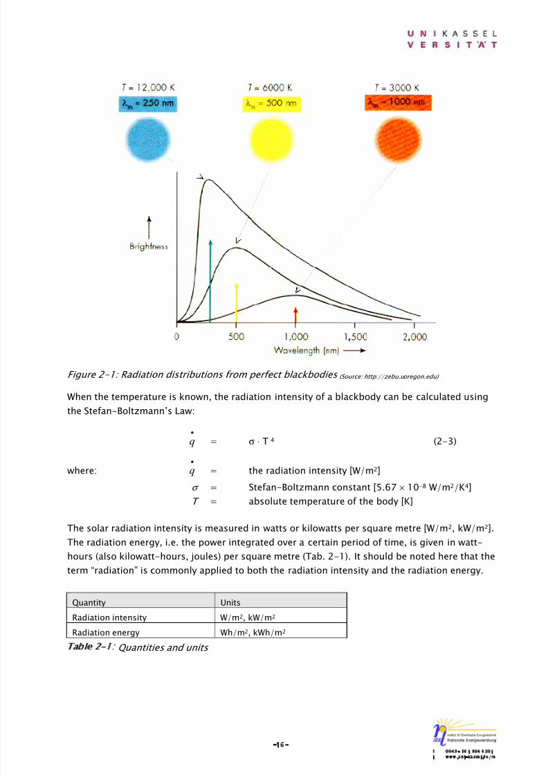
Figure 2-1: Radiation distributions from perfect blackbodies (Source: http://zebu.uoregon.edu)
When the temperature is known, the radiation intensity of a blackbody can be calculated using
the Stefan-Boltzmann’s Law:
•
q = σ ⋅ T 4 (2-3)
where:•
q = the radiation intensity [W/m2]
σ = Stefan-Boltzmann constant [5.67 × 10⁻⁸ W/m2/K4]
T = absolute temperature of the body [K]
The solar radiation intensity is measured in watts or kilowatts per square metre [W/m2, kW/m2].
The radiation energy, i.e. the power integrated over a certain period of time, is given in watt-hours (also kilowatt-hours, joules) per square metre (Tab. 2-1). It should be noted here that the
term “radiation” is commonly applied to both the radiation intensity and the radiation energy.
Quantity Units
Radiation intensity W/m2, kW/m2
Radiation energy Wh/m2, kWh/m2
Table 2-1: Quantities and units

8/14/2019 Photovoltaic Systems Technology SS 2003
http://slidepdf.com/reader/full/photovoltaic-systems-technology-ss-2003 21/155
-17-t 0049- 561 804 6201i www.uni-kassel.de/re
2.2 Solar Radiation outside the Earth’s Atmosphere
The radiation intensity of the Sun varies from the center to its surface. The outgoing radiant
flux spreads out over sphere’s surface. It is therefore weaker with the square of distance from
the Sun. Due to an extremely large mean distance between the Sun and the Earth the beam
radiation received on the Earth is almost parallel. Measurements indicate that the radiant flux,
received from the Sun outside the Earth’s atmosphere is remarkably constant. The so-called
solar constant , 1367 W/m2, defines the average amount of energy received in a unit of time on
a unit area perpendicular to the path of the radiation outside the atmosphere at the average
distance of the Earth’s orbit around the Sun. This value fluctuates with a few percent resulted
especially from the change of Sun-Earth distance in the orbit during a year [2].
Additionally an approximate value of solar constant can be also derived according to the
following principle: Assume the Sun to be a blackbody. In consequence of energy conservation,
its outgoing radiant flux passes through any imaginary external spherical surface concentric to
the Sun (Fig. 2-2). In particular, this flux passes through a surface of radius equal to the
average distance between Earth and Sun. The flux density observed at this distance is defined
as the solar constant.
Figure 2-2: Schematic geometry of the Sun-Earth relationships
The radiant flux at the Sun’s surface = The radiant flux at the Earth’s orbit
surfaceSunsurfaceSun A q ⋅
•
= orbit Earth0 A S ⋅
where: surfaceSunq
•
= solar radiation at the Sun’s surface [W/m2]
0S = solar constant [W/m2]
ASun surface = area of the Sun’s surface [m2]
AEarth orbit = area of a sphere at the Earth orbit [m2]
R Earth = 6378 km
R Sun = 695000 kmR Earth orbit = 149 million km

8/14/2019 Photovoltaic Systems Technology SS 2003
http://slidepdf.com/reader/full/photovoltaic-systems-technology-ss-2003 22/155
-18-t 0049- 561 804 6201i www.uni-kassel.de/re
Thus, 0S = orbit Earth
surfaceSun
surfaceSun A
A q ⋅
•
=
( )
( )2orbit Earth
2
Sun4
surfaceSun R4
R4 T π
π σ ⋅⋅
=
( ) 10149
106955762105.67
2
9
6 48-
×
×⋅⋅×
= 1360 W/m2
Since R Earth orbit is not fully constant, S 0 changes slightly throughout a year (1300 W/m2 < S 0 <
1390 W/m2).
2.3 Solar Radiation on the Earth’s Surface
The radiation intensity outside the Earth’s atmosphere according to the solar constant is called
the extraterrestrial radiation . The maximum of the spectral distribution is situated in the area
of visible light with a wavelength of 0.38 µm until 0.78 µm and drop steeply out one side to
ultraviolet- (UV: 0.2 - 0.38 µm) and the other side to infrared radiation (IR: 0.78 - 2.6 µm) as
illustrated in Figure 2-3.
0
250
500
750
1,000
1,250
1,500
1,750
2,000
2,250
0 200 400 600 800 1,000 1,200 1,400 1,600 1,800 2,000
Wavelength [nm]
S p e c t r a l d i s t r i b u i t i o n
[ W / m 2 /µ m
]
Cloudy sky Clear sky Extraterestrial radiation
UV visible IR
O2 , H2O
H2O
O3
H2O, CO2
Figure 2-3: Spectral distribution of solar radiation (Source: Kassel University)
Regarding light falling on a surface of glass it can be reflected ( ρ ), absorbed (α ) or transmitted
(τ ) [1], whereby
8/14/2019 Photovoltaic Systems Technology SS 2003
http://slidepdf.com/reader/full/photovoltaic-systems-technology-ss-2003 23/155
-19-t 0049- 561 804 6201i www.uni-kassel.de/re
ρ + α + τ = 1 (2-4)
Similarly, while passing through the atmosphere, the extraterrestrial radiation experiences
attenuation such as reflection, scattering (reflection in many directions) and absorption. The
solar radiation is reflected and scattered primarily by clouds (moisture and ice particles),
particulate matter (dust, smoke, haze and smog) and various gases. Reflection of incident solar
radiation back into space by clouds varies with their thickness and albedo (ratio of reflected to
incident light). Thin clouds may reflect less than 20 % of the incident solar radiation whereas a
thick and dense cloud may reflect over 80 % [5]. Consequently, regions with cloudy climates
receive less solar radiation than cloud-free desert climates. For any given location, the solar
radiation reaching the Earth’s surface decreases with increasing cloud cover.
In addition, local geographical features such as mountains, oceans and large lakes influence the
formation of clouds. Therefore the amount of solar radiation received for these areas may be
different from that received by land areas located a short distance away. For example,
mountains may receive less solar radiation than nearby foothills and plains located a shortdistance away. Winds blowing against mountains force some of the air to rise and clouds form
from the moisture in the air as it cools. Coastlines may also receive a different amount of solar
radiation than areas further inland. Where the changes in geography are less pronounced, e.g.
in the Great Plains, the amount of solar radiation varies less [6].
The two major processes involved in tropospheric scattering are determined by the size of the
molecules and particles. They are known as selective scattering and nonselective scattering .
Selective scattering is caused by smoke, fumes, haze and gas molecules that are the same size
or smaller than the incident radiation wavelength. Scattering in these cases is inversely
proportional to wavelength and is therefore most effective for the shortest wavelengths (bluecomponents).
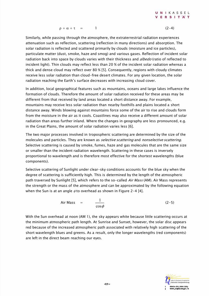
Selective scattering of Sunlight under clear-sky conditions accounts for the blue sky when the
degree of scattering is sufficiently high. This is determined by the length of the atmospheric
path traversed by Sunlight [5], which refers to the so-called Air Mass (AM). Air Mass represents
the strength or the mass of the atmosphere and can be approximated by the following equation
when the Sun is at an angle φ to overhead as shown in Figure 2-4 [4].
Air Mass =
φ cos
1(2-5)
With the Sun overhead at noon (AM 1), the sky appears white because little scattering occurs at
the minimum atmospheric path length. At Sunrise and Sunset, however, the solar disc appears
red because of the increased atmospheric path associated with relatively high scattering of the
short wavelength blues and greens. As a result, only the longer wavelengths (red components)
are left in the direct beam reaching our eyes.
8/14/2019 Photovoltaic Systems Technology SS 2003
http://slidepdf.com/reader/full/photovoltaic-systems-technology-ss-2003 24/155
-20-t 0049- 561 804 6201i www.uni-kassel.de/re
Figure 2-4: Effect of the Earth’s atmosphere on the solar radiation
Nonselective scattering is caused by dust, fog and clouds with particle sizes more than 10
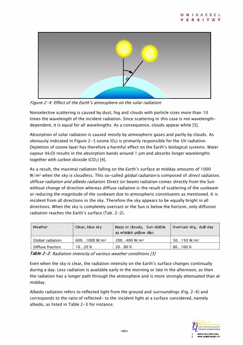
times the wavelength of the incident radiation. Since scattering in this case is not wavelength-dependent, it is equal for all wavelengths. As a consequence, clouds appear white [5].
Absorption of solar radiation is caused mostly by atmospheric gases and partly by clouds. As
obviously indicated in Figure 2-3 ozone (O3) is primarily responsible for the UV radiation.
Depletion of ozone layer has therefore a harmful effect on the Earth’s biological systems. Water
vapour (H2O) results in the absorption bands around 1 µm and absorbs longer wavelengths
together with carbon dioxide (CO2) [4].
As a result, the maximal radiation falling on the Earth’s surface at midday amounts of 1000
W/m2 when the sky is cloudless. This so-called global radiation is composed of direct radiation ,
diffuse radiation and albedo radiation . Direct (or beam) radiation comes directly from the Sunwithout change of direction whereas diffuse radiation is the result of scattering of the sunbeam
or reducing the magnitude of the sunbeam due to atmospheric constituents as mentioned. It is
incident from all directions in the sky. Therefore the sky appears to be equally bright in all
directions. When the sky is completely overcast or the Sun is below the horizon, only diffusion
radiation reaches the Earth’s surface (Tab. 2-2).
Weather Clear, blue sky Hazy or cloudy, Sun visible
as whitish yellow disc
Overcast sky, dull day
Global radiation 600…1000 W/m2
200…400 W/m2
50…150 W/m2
Diffuse fraction 10…20 % 20…80 % 80…100 %
Table 2-2: Radiation intensity of various weather conditions [3]
Even when the sky is clear, the radiation intensity on the Earth’s surface changes continually
during a day. Less radiation is available early in the morning or late in the afternoon, as then
the radiation has a longer path through the atmosphere and is more strongly attenuated than at
midday.
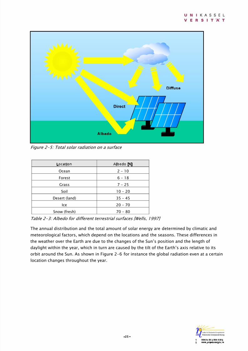
Albedo radiation refers to reflected light from the ground and surroundings (Fig. 2-6) and
corresponds to the ratio of reflected- to the incident light at a surface considered, namely
albedo, as listed in Table 2-3 for instance.
φ
8/14/2019 Photovoltaic Systems Technology SS 2003
http://slidepdf.com/reader/full/photovoltaic-systems-technology-ss-2003 25/155
-21-t 0049- 561 804 6201i www.uni-kassel.de/re
Figure 2-5: Total solar radiation on a surface
Location Albedo [%]
Ocean 2 - 10
Forest 6 - 18
Grass 7 - 25Soil 10 - 20
Desert (land) 35 - 45
Ice 20 - 70
Snow (fresh) 70 - 80
Table 2-3: Albedo for different terrestrial surfaces [Wells, 1997]
The annual distribution and the total amount of solar energy are determined by climatic and
meteorological factors, which depend on the locations and the seasons. These differences in
the weather over the Earth are due to the changes of the Sun’s position and the length of
daylight within the year, which in turn are caused by the tilt of the Earth’s axis relative to its
orbit around the Sun. As shown in Figure 2-6 for instance the global radiation even at a certain
location changes throughout the year.
Direct
8/14/2019 Photovoltaic Systems Technology SS 2003
http://slidepdf.com/reader/full/photovoltaic-systems-technology-ss-2003 26/155
-22-t 0049- 561 804 6201i www.uni-kassel.de/re
0.0
1.0
2.0
3.0
4.0
5.0
6.0
7.0
8.0
Jan Feb Mar Apr May Jun Jul Aug Sep Oct Nov Dec Mean
Month
A v e r a g e d a i l y g l o b a l r a d i a t i o n
[ k W h
/ m 2 ]
Maximum Mean Minimum
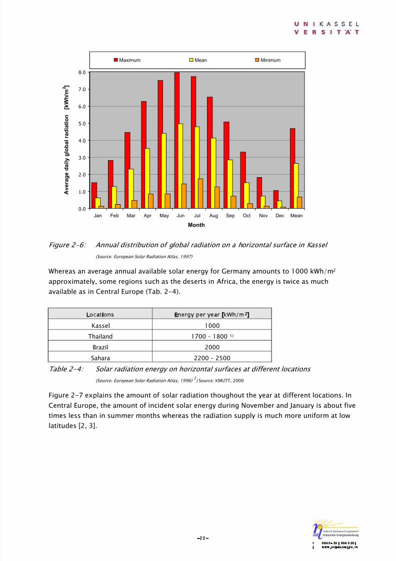
Figure 2-6: Annual distribution of global radiation on a horizontal surface in Kassel
(Source: European Solar Radiation Atlas, 1997)
Whereas an average annual available solar energy for Germany amounts to 1000 kWh/m2
approximately, some regions such as the deserts in Africa, the energy is twice as much
available as in Central Europe (Tab. 2-4).
Locations Energy per year [kWh/m2]
Kassel 1000
Thailand 1700 – 1800 1)
Brazil 2000
Sahara 2200 – 2500
Table 2-4: Solar radiation energy on horizontal surfaces at different locations
(Source: European Solar Radiation Atlas, 1996) 1 ) Source: KMUTT, 2000
Figure 2-7 explains the amount of solar radiation thoughout the year at different locations. InCentral Europe, the amount of incident solar energy during November and January is about five
times less than in summer months whereas the radiation supply is much more uniform at low
latitudes [2, 3].

8/14/2019 Photovoltaic Systems Technology SS 2003
http://slidepdf.com/reader/full/photovoltaic-systems-technology-ss-2003 27/155
-23-t 0049- 561 804 6201i www.uni-kassel.de/re
Figure 2-7: Annual distribution of solar radiation at different locations
(Source: European Solar Radiation Atlas 1996, Solar Energy Research and Training Center)
In addition, annual mean solar radiation for all lands over the world is presented in Figure 2-8.
Here it is obviously seen that the amount of incident solar radiation is different in each part of
the world.
Figure 2-8: Annual mean solar radiation 1961-1990 in kWh/m 2 a
(Source: Intergovernmental Panel on Climate Change)
Fortaleza
Kassel
Pitsanulok
0,0
1,0
2,0
3,0
4,0
5,0
6,0
7,0
8,0
Jan Feb Mar Apr May Jun Jul Aug Sep Oct Nov Dec Mean
Month
A
v e r a g e d a i l y g l o b a l r a d i a t i o n [ k W h / m
2 ]
Fortaleza - Brazil Kassel - Germany Pitsanulok - Thailand

8/14/2019 Photovoltaic Systems Technology SS 2003
http://slidepdf.com/reader/full/photovoltaic-systems-technology-ss-2003 28/155
-24-t 0049- 561 804 6201i www.uni-kassel.de/re
2.4 Greenhouse Effect
Satellite measurement confirmed that the radiation balance took place at the boundary of the
atmosphere, i.e. the solar energy received by the Earth balances the energy lost by the Earth
back into space. According to the geometric Sun-Earth relationship (Fig. 2-2) energy absorbed
by the Earth is considered only in area projected against the Sun’s rays (= π⋅ R Earth 2 ). However,
the Earth reradiates energy with its whole surface area (= 4 π⋅ R Earth 2 ). To avoid confusion with
W/m2, it must be here noted that all amounts of solar radiation in the following figure will refer
to solar radiation power and thus be calculated in PW (Peta Watt = 1015 W).
Figure 2-9: Radiation and energy balance in PW [7]
As indicated in Figure 2-9, 30 % of incoming solar radiation at the boundary of the atmosphere
is reflected to space (the Earth’s average albedo from both the atmosphere and the surface): the
biggest part is reflected by clouds, other part by air molecules and aerosols (tiny smoke
particles) and the rest by the Earth’s surface. Approx. 20 % (33 PW) is absorbed in the
atmosphere whereas about 26 PW is absorbed by atmospheric gas, i.e. H2O, CO2 and the other7 PW by clouds. As a result, the rest 50 % (90 PW) is incident on the Earth’s surface
corresponding to the global radiation, which consists of direct-, diffuse-, and albedo
components as mentioned before and warms it up. In comparison to the world primary energy
consumption [2000] of 114 PWh the annual incident solar radiation is nearly 7000 times
greater.
The amount of 70 % of the incoming radiation, which stay in the “Earth-atmosphere” system,
has to be radiated again back to space. The higher the temperature of a body, the higher the
frequency or the longer the wavelength of the energy radiated. Since the Earth’s surface and
atmosphere (with 288 K) are much colder than the Sun’s surface (with 5762 K), the Earthradiates less energy than the Sun and the energy has longer wavelengths (Fig. 2-10).
Sensibl longwaveCounter-Latent
Absorbedby clouds
Absorbed
by gases
Incoming solar
Surface
Thermal absorption and emissionin the atmos here

8/14/2019 Photovoltaic Systems Technology SS 2003
http://slidepdf.com/reader/full/photovoltaic-systems-technology-ss-2003 29/155
-25-t 0049- 561 804 6201i www.uni-kassel.de/re
Figure 2-10: Spectral distribution of the Sun and the Earth (Source: Kassel University)
According to the Figure 2-9 the amount of longwave radiation emitted from the Earth’s surface
is surprisingly more than the incoming solar radiation. This is due to the energy exchange in
the Earth-atmosphere system. Whereas 10 PW passes directly through the atmosphere into
space, a big part of longwave surface radiation (180 PW) is however absorbed by theatmospheric molecules: if the frequency of the radiation is compatible with the molecule’s
rotational frequency or with the frequency, at which the molecule vibrates, then the molecule
can absorb the radiation resulting in increase of the molecule’s rotational frequency or more
vigorously vibration respectively. This absorption is largely due to two gases: water vapor
(moisture) and carbon dioxide (CO2). For example, CO2 molecule has vibration that allows the
molecule to absorb IR at wavelength of 15 µm, which is near the wavelength of the majority of
Earth’s outgoing IR.
Having absorbed this IR, the atmosphere becomes a radiator and therefore emits longwave
energy. This heat is emitted in all directions: 113 PW is released to outer space, however its
substantial part is headed downward to the surface (152 PW). The portion of atmospheric
radiation that is returned to Earth is called counterradiation . As a result, the net radiation loss
of the Earth’s surface amounts to 38 PW. This screening effect of the atmosphere is generally
well known as greenhouse effect whereas vapour, CO2 and other gases such as O3, methane
(CH4), nitrous oxide (N2O) and others, which contribute to this process, are therefore referred to
greenhouse gases .
Regarding energy balance at the Earth’s surface, the difference between the absorbed
shortwave- and emitted longwave radiation is therefore 52 PW. This gap is closed after taking
latent- and sensible heat (40 PW and 12 PW respectively) into account. Sensible heat can be
measured by thermometer. It is transferred through conduction, convection and advection:
when surface is heated by the incident solar radiation, the nearby layer of air is warmed up
0
250
500
750
1.000
1.250
1.500
1.750
2.000
2.250
0 2.000 4.000 6.000 8.000 10.000 12.000 14.000 16.000 18.000 20.000
Wavelength [nm]
S u n - S p e c t r a l I r r a d i a n c e
[ W / m 2 µ m ]
0
25
50
75
100
125
150
175
200
225
E a r t h - S p e c t r a l I r r a d i a n c e
[ W / m 2 µ m ]
5762 K 288 K
8/14/2019 Photovoltaic Systems Technology SS 2003
http://slidepdf.com/reader/full/photovoltaic-systems-technology-ss-2003 30/155
-26-t 0049- 561 804 6201i www.uni-kassel.de/re
through conduction and this warmth is then transferred upward through convection whereas
advection is horizontal convection.
Latent heat is taken up or released on a phase change of water between three forms, i.e. ice,
water and vapour. When water is evaporated from oceans, rivers or moist soils, latent heat of
vaporization is taken up by the resulting vapour. When water vapor condenses to form clouds,the same amount of latent heat is released to the atmosphere.
As a result, the radiation balance at boundary of the atmosphere is completed. Furthermore,
according to Figure 2-9 and by assuming the Earth as a blackbody, the effective radiating
temperature of the Earth (T ) as view from outer space can be derived from total heat radiated
out of the boundary of the atmosphere:
σ ⋅ T4 = (113+10)/4π⋅REarth2
T = 255 K = -18 °C or 0 °F
However, Earth’s average surface temperature is 288 K or 15 °C. The cause of difference
between the effective radiating temperature and the global average surface temperature lies in
the existence of the atmosphere, namely the greenhouse effect. This so-called natural
greenhouse effect warms the surface by 33 °C resulting in a livable climate on Earth [7, 8, 9].
However, since 1860, the beginning of systematic meteorological recording, the global average
temperature has increased approx. 0.6 °C. Nevertheless it is concerned with to the strongest
rise in temperature in the northern Earth’s hemisphere during the past 1,000 years.
Moreover, by means of abundance of scientific studies today it can be already proved that ourclimate has changed in the past two centuries substantially: sea level increased approx. 10 to
20 cm in the past century. Snow cover sank ca. 10 % since 1960. In the 20th century
precipitation in the central and higher latitude increased about 0.5 to 1 % per year.
This leaded especially in the past century to the fact that more often and intensive drought took
place in some parts of Africa and Asia. In the Pacific Ocean, since 1970, more often, longer
continual and intensive temperature anomalies with frequent unfavourable effects to the
mankind’s health, to settlement, to the agriculture and forestry and others are observed.
The rising temperature above that occurring related to the natural greenhouse effect refers to
the enhanced greenhouse effect caused by increase in concentration of the greenhouse gases in
the atmosphere.
Since the industrialization CO2 increased in concentration about 30 %. The meanwhile reached
level (367 ppm in comparison to 280 ppm before the industrialization) as well as the topical
increasing rate (at present, ca. 1.5 ppm per year) is unique for the last 20,000 years. If one
considers far back to the past, no comparable concentration during the last 420,000 years and
no comparable increase speed during the last 20,000 years are not found.
The concentration of CH4 rose more than double. Such a concentration level had not also been
reached in the last 420,000 years. Similarly, the concentration of N2O increased ca. 17 % and
8/14/2019 Photovoltaic Systems Technology SS 2003
http://slidepdf.com/reader/full/photovoltaic-systems-technology-ss-2003 31/155
-27-t 0049- 561 804 6201i www.uni-kassel.de/re
goes on rising. Such a concentration had never appeared according to our knowledge
circumstance in the past 1,000 years.
These increases in concentration of the greenhouse gases are caused almost exclusively by
mankind’s activities, namely the combustion of fossil fuels (coal, gas, oil), deforestation and
particular agricultural methods (since ca. 1750).
As a result, more heat is trapped by the atmosphere and has a consequence that more heat is
reradiated downward to the surface (counterradiation) and therefore contributes to global
warming. However the word "enhanced" is usually omitted, but it should not be forgotten in
discussions of the greenhouse effect [10].
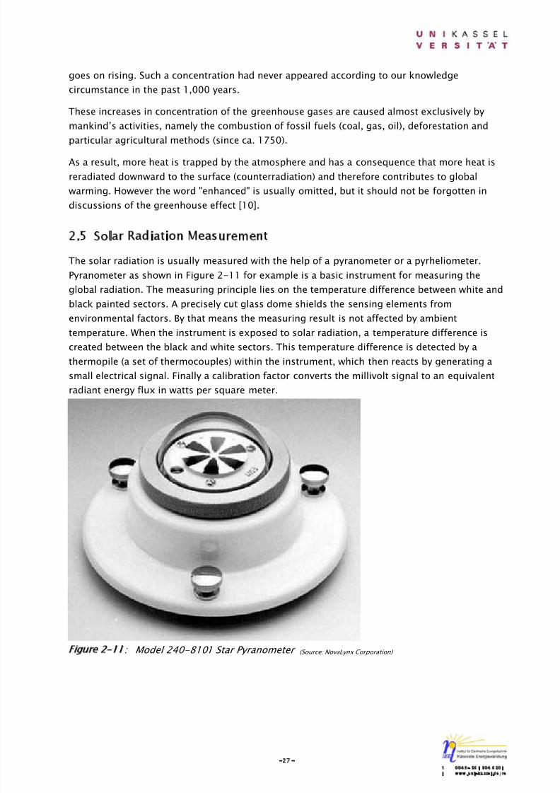
2.5 Solar Radiation Measurement
The solar radiation is usually measured with the help of a pyranometer or a pyrheliometer.
Pyranometer as shown in Figure 2-11 for example is a basic instrument for measuring theglobal radiation. The measuring principle lies on the temperature difference between white and
black painted sectors. A precisely cut glass dome shields the sensing elements from
environmental factors. By that means the measuring result is not affected by ambient
temperature. When the instrument is exposed to solar radiation, a temperature difference is
created between the black and white sectors. This temperature difference is detected by a
thermopile (a set of thermocouples) within the instrument, which then reacts by generating a
small electrical signal. Finally a calibration factor converts the millivolt signal to an equivalent
radiant energy flux in watts per square meter.
Figure 2-11: Model 240-8101 Star Pyranometer (Source: NovaLynx Corporation)
8/14/2019 Photovoltaic Systems Technology SS 2003
http://slidepdf.com/reader/full/photovoltaic-systems-technology-ss-2003 32/155
-28-t 0049- 561 804 6201i www.uni-kassel.de/re
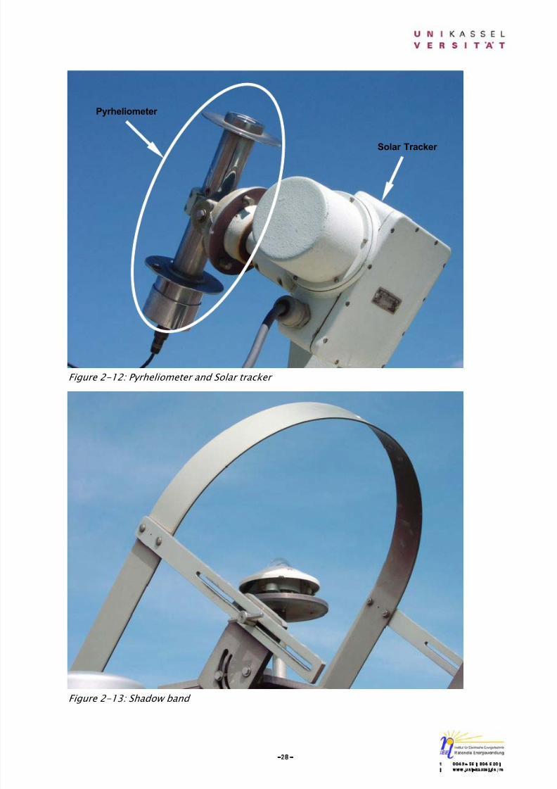
Figure 2-12: Pyrheliometer and Solar tracker
Figure 2-13: Shadow band
Solar Tracker
Pyrheliometer
8/14/2019 Photovoltaic Systems Technology SS 2003
http://slidepdf.com/reader/full/photovoltaic-systems-technology-ss-2003 33/155
-29-t 0049- 561 804 6201i www.uni-kassel.de/re
Direct radiation can be measured by pyrheliometer. In contrast to a pyranometer, the black
sensor disc is located at the base of a tube whose axis is aligned with the direction of the
sunbeam. Thus, diffuse radiation is essentially blocked from the sensor surface. Furthermore,
pyrheliometer is normally mounted on a solar tracker so that it is continually pointed directly at
the Sun throughout the day (Fig. 2-12). However, this makes the measurements complicate and
expensive.
In case of the diffuse radiation, it can be determined by subtracting the measured direct
radiation from the global radiation mathematically. However, it can also be measured by
applying a shadow band to the pyranometer as presented in Figure 2-13. By this means, the
sunbeam is blocked and whereby a value measured refers only to the diffuse component.
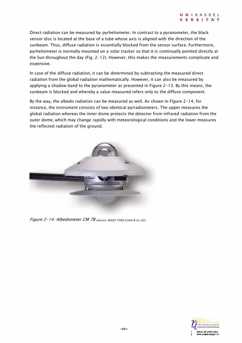
By the way, the albedo radiation can be measured as well. As shown in Figure 2-14, for
instance, the instrument consists of two identical pyrradiometers. The upper measures the
global radiation whereas the inner dome protects the detector from infrared radiation from the
outer dome, which may change rapidly with meteorological conditions and the lower measuresthe reflected radiation of the ground.
Figure 2-14: Albedometer CM 7B (Source: ADOLF THIES GmbH & Co. KG)
8/14/2019 Photovoltaic Systems Technology SS 2003
http://slidepdf.com/reader/full/photovoltaic-systems-technology-ss-2003 34/155
-30-t 0049- 561 804 6201i www.uni-kassel.de/re
2.6 References
[1] Schmid, J.: Script for the lecture: Energiemanagement in Gebäudebereich; Kassel
University. pg. 45-51.
[2] Schmid, J.: Photovoltaik: ein Leitfaden für die Praxis; ein Informationspaket; Köln: Verl.
TÜV Rheinland, 1995. pg. 10-12.
[3] Kaiser, R.: Fundamentals of solar energy use. In: Fraunhofer Institute for Solar Energy
Systems: Course book for the seminar: Photovoltaic Systems; Freiburg, 1995. pg. 56-
63.
[4] Wenham, S.R.; Green, M.A.; Watt, M.E.: Applied Photovoltaics; Australia. pg. 1-19.
[5] Acra, A.; Jurdi, M.; Mu'allem, H.; Karahagopian, Y.; Raffoul, Z.: Water Disinfection bySolar Radiation: Assessment and Application; Ottawa, Canada: IDRC, 1990.
[6] Andrew, Marsh: Script for the lecture: Solar Radiation; University of Western Australia.
[7] Grünhage, Ludger: Script for the lecture: Pflanzeökologie I: Strahlungsbilanz
verschiedener Oberflächen; Giessen University. pg. 15-19.
[8] Marshall, John: Script for the lecture: Physics of Atmospheres and Oceans: The global
energy balance; Massachusetts Institute of Institute, USA.
[9] Naumov, Aleksev: Script for the lecture: Physical Environmental Geography: Insolation
and temperature – Earth’s global energy balance; State University of New York at
Buffalo, USA.
[10] Umweltbundesamt: Klimaschutz 2001: Tatsachen - Risiken - Handlungs-
möglichkeiten; Berlin, 2001. pg. 2-3.

8/14/2019 Photovoltaic Systems Technology SS 2003
http://slidepdf.com/reader/full/photovoltaic-systems-technology-ss-2003 35/155
-31-t 0049- 561 804 6201i www.uni-kassel.de/re
3 FUNDAMENTALS OF PHOTOVOLTAICS
3.1 Introduction
The direct transformation from the solar radiation energy into electrical energy is possible with
the photovoltaic effect by using solar cells . The term photovoltaic is often abbreviated to PV.
The radiation energy is transferred by means of the photoeffect directly to the electrons in their
crystals. With the photovoltaic effect an electrical voltage develops in consequence of the
absorption of the ionizing radiation. Solar cells must be differentiated from photocells whose
conductivity changes with irradiation of sunlight. Photocells serve e.g. as exposure cells in
cameras since their electrical conductivity can drastically vary with small intensity changes.
They produce however no own electrical voltage and need therefore a battery for operation.
The photovoltaic effect was discovered in 1839 by Alexandre Edmond Becquerel while
experimenting with an electrolytic cell made up of two metal electrodes. Becquerel found that
certain materials would produce small amounts of electric current when exposed to light. About
50 years later Charles Fritts constructed the first true solar cells using junctions formed by
coating the semiconductor selenium with an ultrathin, nearly transparent layer of gold. Fritts’s
devices were very inefficient: efficiency less than 1 %.
The first silicon solar cell with an efficiency of approx. 6% was developed in 1954 by three
American researchers, namely Daryl Chapin, Calvin Fuller and G.L. Pearson in the Bell
Laboratories. Solar cells proved particularly suitably for the energy production for satellites in
space and still represent today the exclusive energy source of all space probes. The interest in
terrestrial applications has increased since the oil crisis in 1973. Main objective of research and
development is thereby a drastic lowering of the manufacturing costs and lately also a
substantial increase of the efficiency.
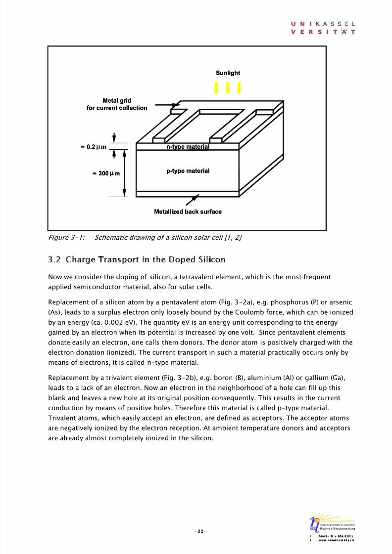
The base material of almost all solar cells for applications in space and on earth is silicon. The
most common structure of a silicon solar cell is schematically represented in Figure 3-1:
An approx. 300 µm silicon wafer consists of two layers with different electrical properties
prepared by doping foreign atoms such as boron and phosphorous. The back surface side is
total metallized for charge carrier collection whereas on the front, which exposes to the beam
of incident light, only one metal grid is applied in order that as much light as possible canpenetrate into the cell. The surface is normally provided with an antireflection coating to keep
the losses from reflection as small as possible.
8/14/2019 Photovoltaic Systems Technology SS 2003
http://slidepdf.com/reader/full/photovoltaic-systems-technology-ss-2003 36/155
-32-t 0049- 561 804 6201i www.uni-kassel.de/re
Figure 3-1: Schematic drawing of a silicon solar cell [1, 2]
3.2 Charge Transport in the Doped Silicon
Now we consider the doping of silicon, a tetravalent element, which is the most frequent
applied semiconductor material, also for solar cells.
Replacement of a silicon atom by a pentavalent atom (Fig. 3-2a), e.g. phosphorus (P) or arsenic
(As), leads to a surplus electron only loosely bound by the Coulomb force, which can be ionized
by an energy (ca. 0.002 eV). The quantity eV is an energy unit corresponding to the energy
gained by an electron when its potential is increased by one volt. Since pentavalent elements
donate easily an electron, one calls them donors. The donor atom is positively charged with the
electron donation (ionized). The current transport in such a material practically occurs only by
means of electrons, it is called n-type material.
Replacement by a trivalent element (Fig. 3-2b), e.g. boron (B), aluminium (Al) or gallium (Ga),
leads to a lack of an electron. Now an electron in the neighborhood of a hole can fill up thisblank and leaves a new hole at its original position consequently. This results in the current
conduction by means of positive holes. Therefore this material is called p-type material.
Trivalent atoms, which easily accept an electron, are defined as acceptors. The acceptor atoms
are negatively ionized by the electron reception. At ambient temperature donors and acceptors
are already almost completely ionized in the silicon.
≈ 0.2 µm
Sunlight
Metal grid
for current collection
Metallized back surface
p-type material
n-type material
≈ 300 µm
≈ 0.2 µm
Sunlight
Metal grid
for current collection
Metallized back surface
p-type material
n-type material
≈ 300 µm

8/14/2019 Photovoltaic Systems Technology SS 2003
http://slidepdf.com/reader/full/photovoltaic-systems-technology-ss-2003 37/155
-33-t 0049- 561 804 6201i www.uni-kassel.de/re
Figure 3-2: Doping of silicon (a) with pentavalent atom (b) with trivalent atom
3.3 Effects of a P-N Junction
Usually a p-n junction is generated by the fact that a strong n-type layer is produced in the p-
type material by indiffusion of a donor (P, As) at higher temperatures (ca. 850 °C). Completely
analog in the n-type material, although less common, a p-n junction can be produced by
indiffusion of an acceptor.
In the boundary surface’s neighborhood of the n- or p-type material the following effects
occur: In the n-region so many electrons are available, in the p-region so many holes. These
concentration differences lead to the fact that electrons from the n-region diffuse into the p-
region and holes from the p-region diffuse into the n-region. As a result, diffusion currents of
electrons into the p-region and diffusion currents of holes into the n-region arise (Fig. 3-3).
By the flow of negative and positive charges a deficit of charges develops within the before
electrically neutral regions, i.e. it results a positive charge within the donor region and a
negative charge within the acceptor region. Thus an electrical field develops over the boundary
surface and causes now field currents from both charge carrier types, which are against the
diffusion currents. In the equilibrium the total value of current through the boundary surface is
zero. The field currents compensate completely the diffusion currents: the hole currents
compensate completely among themselves and the electron currents likewise.
(b)(a)
free
electronhole
P
Si
Si
SiSi
Si Si
SiSi
B
Si
Si
SiSi
Si Si
SiSi
(b)(a)
free
electronhole
PP
SiSi
SiSi
SiSiSiSi
SiSi SiSi
SiSiSiSi
BB
SiSi
SiSi
SiSiSiSi
SiSi SiSi
SiSiSiSi

8/14/2019 Photovoltaic Systems Technology SS 2003
http://slidepdf.com/reader/full/photovoltaic-systems-technology-ss-2003 38/155
-34-t 0049- 561 804 6201i www.uni-kassel.de/re
Figure 3-3: Charge carrier distribution at p-n junction and currents through the junction [1]
This electrostatic field extending over the boundary surface refers to the potential difference
V D , which is called diffusion voltage . It is situated in the order of magnitude of 0.8 eV. Thiselectrical field causes the separation of the charge carriers produced by light in the solar cell.
Within the region of the stationary electrical positive and negative charge, in the so-called
space-charge zone , a lack of mobile charge carriers appears, which has very high impedance.
Applying the n-region with a negative voltage (forward bias) reduces the diffusion voltage,
decreases the electrical field strength and thus the field currents. These do not compensate
now the diffusion currents of the electrons and holes, as without external voltage, anymore. As
a result a net diffusion current from electrons and holes flows through the p-n junction. If the
applied voltage is equal to the diffusion voltage, then the field currents disappear and the
current is limited only by the bulk resistors. Contrarily, an applied positive voltage at the
outside n-region (reverse bias) adds itself to the diffusion voltage, increases the space-charge
zone, thus it comes to outweighing the field current. The resulting current whose direction of
the reverse bias is contrary is very small.
The mathematical process at the p-n junction leads to the famous diode equation:
ID =
−
⋅ 1
kT
qV exp I 0 (3-1)
where: I D = diode current [A]
q = magnitude of the electron charge [1.6 ⋅ 10-19 As]V = applied voltage [V]:
holeselectrons
C h
a r g e - c a r r i e r c o n c e n t r a t i o n
stationary
electrical charges
electrons
holesDiffusion current
Field current
Diffusion current
Field current
n-region p-regionp-n junction x
space-charge zone
holeselectrons
C h
a r g e - c a r r i e r c o n c e n t r a t i o n
stationary
electrical charges
electrons
holesDiffusion current
Field current
Diffusion current
Field current
n-region p-regionp-n junction x
space-charge zone
8/14/2019 Photovoltaic Systems Technology SS 2003
http://slidepdf.com/reader/full/photovoltaic-systems-technology-ss-2003 39/155
-35-t 0049- 561 804 6201i www.uni-kassel.de/re
plus = forward bias, minus = reverse bias
k = Boltzmann’s constant [8.65 ⋅ 10-5 eV/K]
T = absolute temperature [K]
The quantity 0 I defines the so-called dark- or saturation current of a diode. It plays a very
large role of the performance of a solar cell.
3.4 Physical Processes in Solar Cells
3.4.1 Optical absorption
Light, which falls on a solar cell, can be reflected, absorbed or transmitted. Since silicon has a
high refractive index (> 3.5), over 30 % of the incident light are reflected. Therefore solar cells
are always provided with an antireflection coating. A thin layer titanium dioxide is usual. Thus
the reflection losses for the solar spectrum can be reduced to about 10 %. More reduction of the reflection losses can be achieved by multi-layer AR layers. A two-part layer from titanium
dioxide and magnesium fluoride reduces the reflection losses of a remainder up to ca. 3 %.
Photons (light quanta) interact with materials mainly by excitation of electrons. The main
process in the field of energy, in which solar cells are applied, is the photoelectric absorption .
Thereby the photon is completely absorbed by a bound electron. The electron takes the entire
energy of the photon and becomes free-electron. However, in semiconductors a photon can be
only absorbed if its energy is larger than the bandgap. Photons with energies smaller than the
bandgap pass through the semiconductor and cannot contribute to an energy conversion.
However, photons with much larger energies than the bandgap are also lost for the energy
conversion since the surplus energy is fast given away as heat to the crystal lattice.
During the interaction of the normal solar spectrum with a silicon solar cell, about 60 % of the
energy for a transformation are lost because many of the photons possess energies, which are
smaller or larger than the bandgap.
3.4.2 Recombination of charge carriers
The absorption of light produces pairs of electrons. The concentration of charge carriers is
therefore higher during the lighting than in the dark. If the light is switched off, the chargecarriers return to their equilibrium concentration in the dark. The return process is called
recombination and is the reverse process for generation by light absorption. Recombination
occurs even naturally also already during the generation. The charge-carrier concentration
appearing with lighting is the result from two opposite running processes.
During their lifetimes the charge carriers can travel a certain distance in the crystal until they
recombine. The average distance, which a charge carrier can travel between the place of its
origin and the place of its recombination, is called diffusion length . This quantity plays an
important role for the behavior of a solar cell [1]. It depends on diffusion coefficient of a
material and a lifetime of a charge carrier (time that it takes for a charge carrier to be captured
according to recombination) [4].
8/14/2019 Photovoltaic Systems Technology SS 2003
http://slidepdf.com/reader/full/photovoltaic-systems-technology-ss-2003 40/155
-36-t 0049- 561 804 6201i www.uni-kassel.de/re
3.4.3 Solar cells under incident light
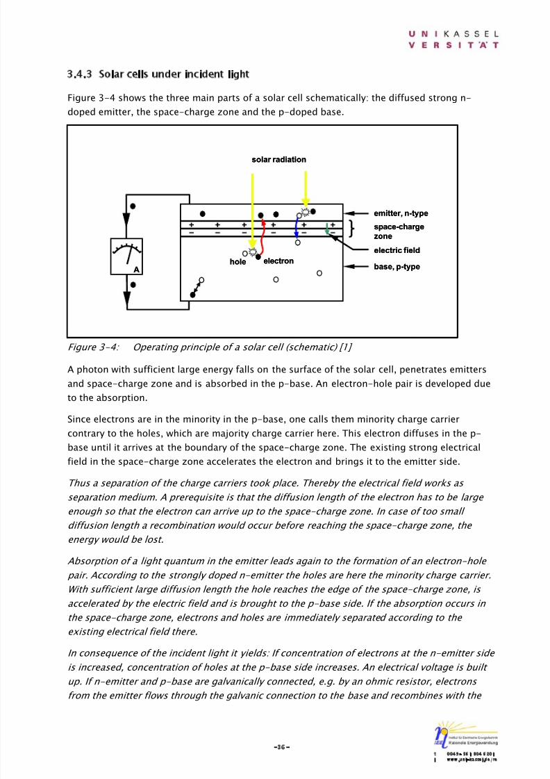
Figure 3-4 shows the three main parts of a solar cell schematically: the diffused strong n-
doped emitter, the space-charge zone and the p-doped base.
Figure 3-4: Operating principle of a solar cell (schematic) [1]
A photon with sufficient large energy falls on the surface of the solar cell, penetrates emitters
and space-charge zone and is absorbed in the p-base. An electron-hole pair is developed due
to the absorption.
Since electrons are in the minority in the p-base, one calls them minority charge carrier
contrary to the holes, which are majority charge carrier here. This electron diffuses in the p-
base until it arrives at the boundary of the space-charge zone. The existing strong electrical
field in the space-charge zone accelerates the electron and brings it to the emitter side.
Thus a separation of the charge carriers took place. Thereby the electrical field works as
separation medium. A prerequisite is that the diffusion length of the electron has to be large
enough so that the electron can arrive up to the space-charge zone. In case of too small
diffusion length a recombination would occur before reaching the space-charge zone, the
energy would be lost.
Absorption of a light quantum in the emitter leads again to the formation of an electron-hole
pair. According to the strongly doped n-emitter the holes are here the minority charge carrier.
With sufficient large diffusion length the hole reaches the edge of the space-charge zone, is
accelerated by the electric field and is brought to the p-base side. If the absorption occurs in
the space-charge zone, electrons and holes are immediately separated according to the
existing electrical field there.
In consequence of the incident light it yields: If concentration of electrons at the n-emitter side
is increased, concentration of holes at the p-base side increases. An electrical voltage is built
up. If n-emitter and p-base are galvanically connected, e.g. by an ohmic resistor, electrons from the emitter flows through the galvanic connection to the base and recombines with the
A
hole electron
solar radiation
emitter, n-type
base, p-type
space-charge
zone
electric field
A
hole electron
solar radiation
emitter, n-type
base, p-type
space-charge
zone
electric field
8/14/2019 Photovoltaic Systems Technology SS 2003
http://slidepdf.com/reader/full/photovoltaic-systems-technology-ss-2003 41/155
-37-t 0049- 561 804 6201i www.uni-kassel.de/re
holes there. Current flow means however power output. This current flow continues so long as
the incident light radiation is available. As a result, light radiation is immediately converted into
electricity [1].
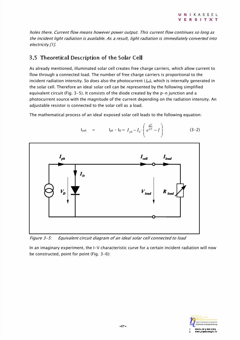
3.5 Theoretical Description of the Solar CellAs already mentioned, illuminated solar cell creates free charge carriers, which allow current to
flow through a connected load. The number of free charge carriers is proportional to the
incident radiation intensity. So does also the photocurrent (I ph ), which is internally generated in
the solar cell. Therefore an ideal solar cell can be represented by the following simplified
equivalent circuit (Fig. 3-5). It consists of the diode created by the p-n junction and a
photocurrent source with the magnitude of the current depending on the radiation intensity. An
adjustable resistor is connected to the solar cell as a load.
The mathematical process of an ideal exposed solar cell leads to the following equation:
Icell = Iph – ID =
−⋅− 1e I I kT
qV
0 ph(3-2)
Figure 3-5: Equivalent circuit diagram of an ideal solar cell connected to load
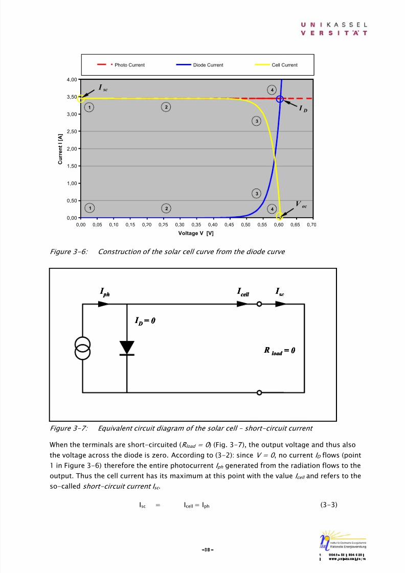
In an imaginary experiment, the I-V characteristic curve for a certain incident radiation will now
be constructed, point for point (Fig. 3-6):
I load
V load
Rload
I cell
I ph
I D
V D
I load
I load
V load
V load
Rload
Rload
I cell
I cell
I ph
I ph
I D
I D
V D
V D
8/14/2019 Photovoltaic Systems Technology SS 2003
http://slidepdf.com/reader/full/photovoltaic-systems-technology-ss-2003 42/155
-38-t 0049- 561 804 6201i www.uni-kassel.de/re
Figure 3-6: Construction of the solar cell curve from the diode curve
Figure 3-7: Equivalent circuit diagram of the solar cell – short-circuit current
When the terminals are short-circuited (R load = 0 ) (Fig. 3-7), the output voltage and thus also
the voltage across the diode is zero. According to (3-2): since V = 0 , no current I D flows (point
1 in Figure 3-6) therefore the entire photocurrent I ph generated from the radiation flows to the
output. Thus the cell current has its maximum at this point with the value I cell and refers to the
so-called short-circuit current I sc .
Isc = Icell = Iph (3-3)
I ph
I sc
I cell
R load = 0
I D = 0
I ph
I ph
I sc
I sc
I cell
I cell
R load = 0 R load = 0
I D = 0 I D = 0
0,00
0,50
1,00
1,50
2,00
2,50
3,00
3,50
4,00
0,00 0,05 0,10 0,15 0,20 0,25 0,30 0,35 0,40 0,45 0,50 0,55 0,60 0,65 0,70
Voltage V [V]
C u r r e n t I [ A ]
Photo Current Diode Current Cell Current
I sc
V oc
1
1
2
2
3
3
4
4
I D
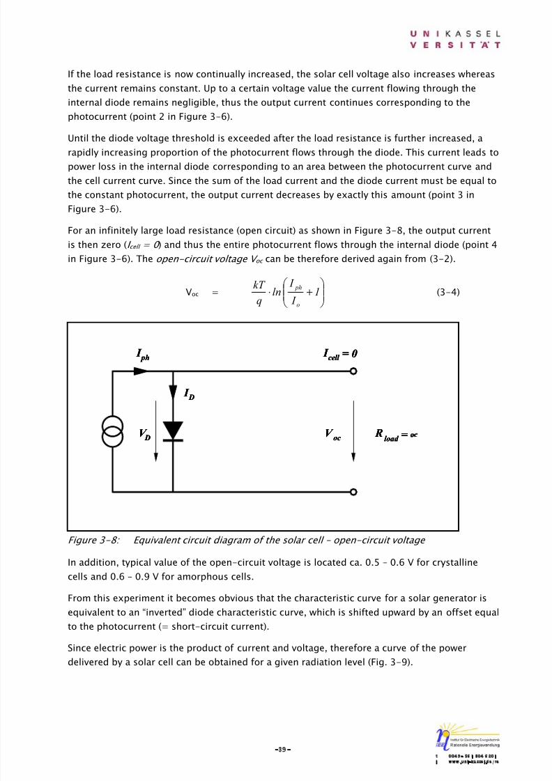
8/14/2019 Photovoltaic Systems Technology SS 2003
http://slidepdf.com/reader/full/photovoltaic-systems-technology-ss-2003 43/155
-39-t 0049- 561 804 6201i www.uni-kassel.de/re
If the load resistance is now continually increased, the solar cell voltage also increases whereas
the current remains constant. Up to a certain voltage value the current flowing through the
internal diode remains negligible, thus the output current continues corresponding to the
photocurrent (point 2 in Figure 3-6).
Until the diode voltage threshold is exceeded after the load resistance is further increased, arapidly increasing proportion of the photocurrent flows through the diode. This current leads to
power loss in the internal diode corresponding to an area between the photocurrent curve and
the cell current curve. Since the sum of the load current and the diode current must be equal to
the constant photocurrent, the output current decreases by exactly this amount (point 3 in
Figure 3-6).
For an infinitely large load resistance (open circuit) as shown in Figure 3-8, the output current
is then zero (I cell = 0 ) and thus the entire photocurrent flows through the internal diode (point 4
in Figure 3-6). The open-circuit voltage V oc can be therefore derived again from (3-2).
Voc =
+⋅ 1
I
I ln
q
kT
o
ph(3-4)
Figure 3-8: Equivalent circuit diagram of the solar cell – open-circuit voltage
In addition, typical value of the open-circuit voltage is located ca. 0.5 – 0.6 V for crystalline
cells and 0.6 – 0.9 V for amorphous cells.
From this experiment it becomes obvious that the characteristic curve for a solar generator is
equivalent to an “inverted” diode characteristic curve, which is shifted upward by an offset equal
to the photocurrent (= short-circuit current).
Since electric power is the product of current and voltage, therefore a curve of the power
delivered by a solar cell can be obtained for a given radiation level (Fig. 3-9).
I cell = 0
V oc
I ph
I D
V D
Rload = ∝
I cell = 0 I cell = 0
V oc
V oc
I ph
I ph
I D
I D
V D
V D
Rload = ∝ Rload = ∝

8/14/2019 Photovoltaic Systems Technology SS 2003
http://slidepdf.com/reader/full/photovoltaic-systems-technology-ss-2003 44/155
-40-t 0049- 561 804 6201i www.uni-kassel.de/re
Figure 3-9: Power curve and maximum power point (MPP) (Source: Kassel University)
Although the current has its maximum at the short-circuit point, the voltage is zero and thus
the power is also zero. The situation for current and voltage is reversed at the open-circuit
point, so again the power here is zero. In between, there is one particular combination of
current and voltage, for which the power reaches a maximum (graphically indicated with an
rectangle area in Figure 3-9). The so-called maximum power point (MPP) represent the working
point, at which the solar cell can deliver maximum power for a given radiation intensity. It issituated near the bend of the I-V characteristic curve. The corresponding values of V MMP and
I MMP can be estimated from V oc and I sc as follows [2]:
In addition, the quantity
FF =( )
( ) scoc
MPP MPP
I V
I V
⋅
⋅(3-5)
is called Fill Factor represents the measure for the quality of the solar cell [4]. It indicates how
far the I-V characteristic curve approximates to a rectangle. Normally the value for crystalline
solar cells is about 0.7-0.8.
The maximum output power of the cell is then
PMPP = VMPP ⋅ IMPP = Voc ⋅ Isc ⋅ FF (3-6)
VMMP ≈ (0.75 – 0.9) Voc
IMMP ≈ (0.85 – 0.95) Isc
0,00
0,50
1,00
1,50
2,00
2,50
3,00
3,50
4,00
0,00 0,05 0,10 0,15 0,20 0,25 0,30 0,35 0,40 0,45 0,50 0,55 0,60 0,65 0,70
Voltage V [V]
C u r r e n t a n d P o w e r . . .
Cell Current [A] Cell Power [W]
V MPP
I MPP
MPP
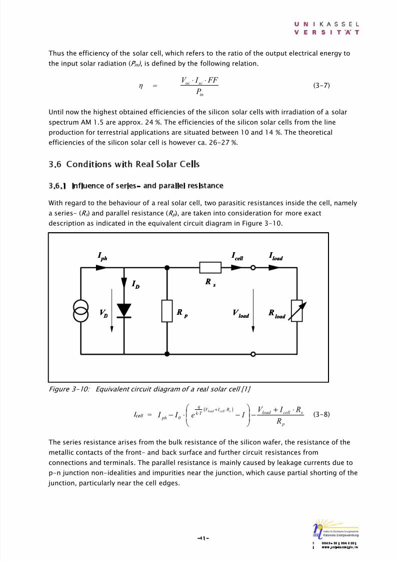
8/14/2019 Photovoltaic Systems Technology SS 2003
http://slidepdf.com/reader/full/photovoltaic-systems-technology-ss-2003 45/155
-41-t 0049- 561 804 6201i www.uni-kassel.de/re
Thus the efficiency of the solar cell, which refers to the ratio of the output electrical energy to
the input solar radiation (P in ) , is defined by the following relation.
η =
in
scoc
P
FF I V ⋅⋅(3-7)
Until now the highest obtained efficiencies of the silicon solar cells with irradiation of a solar
spectrum AM 1.5 are approx. 24 %. The efficiencies of the silicon solar cells from the line
production for terrestrial applications are situated between 10 and 14 %. The theoretical
efficiencies of the silicon solar cell is however ca. 26-27 %.
3.6 Conditions with Real Solar Cells
3.6.1 Influence of series- and parallel resistance
With regard to the behaviour of a real solar cell, two parasitic resistances inside the cell, namely
a series- (R s ) and parallel resistance (R p ), are taken into consideration for more exact
description as indicated in the equivalent circuit diagram in Figure 3-10.
Figure 3-10: Equivalent circuit diagram of a real solar cell [1]
I cell =( )
p
scell load R I V
T k
q
0 ph R
R I V 1e I I
scell load ⋅+−
−⋅−
⋅+⋅⋅ (3-8)
The series resistance arises from the bulk resistance of the silicon wafer, the resistance of the
metallic contacts of the front- and back surface and further circuit resistances from
connections and terminals. The parallel resistance is mainly caused by leakage currents due to
p-n junction non-idealities and impurities near the junction, which cause partial shorting of the
junction, particularly near the cell edges.
I ph
I load
R p
R s
I cell
I D
V D
V load
Rload
I ph
I ph
I load
I load
R p R p
R s
R s
I cell
I cell
I D
I D
V D
V D
V load
V load
Rload
Rload
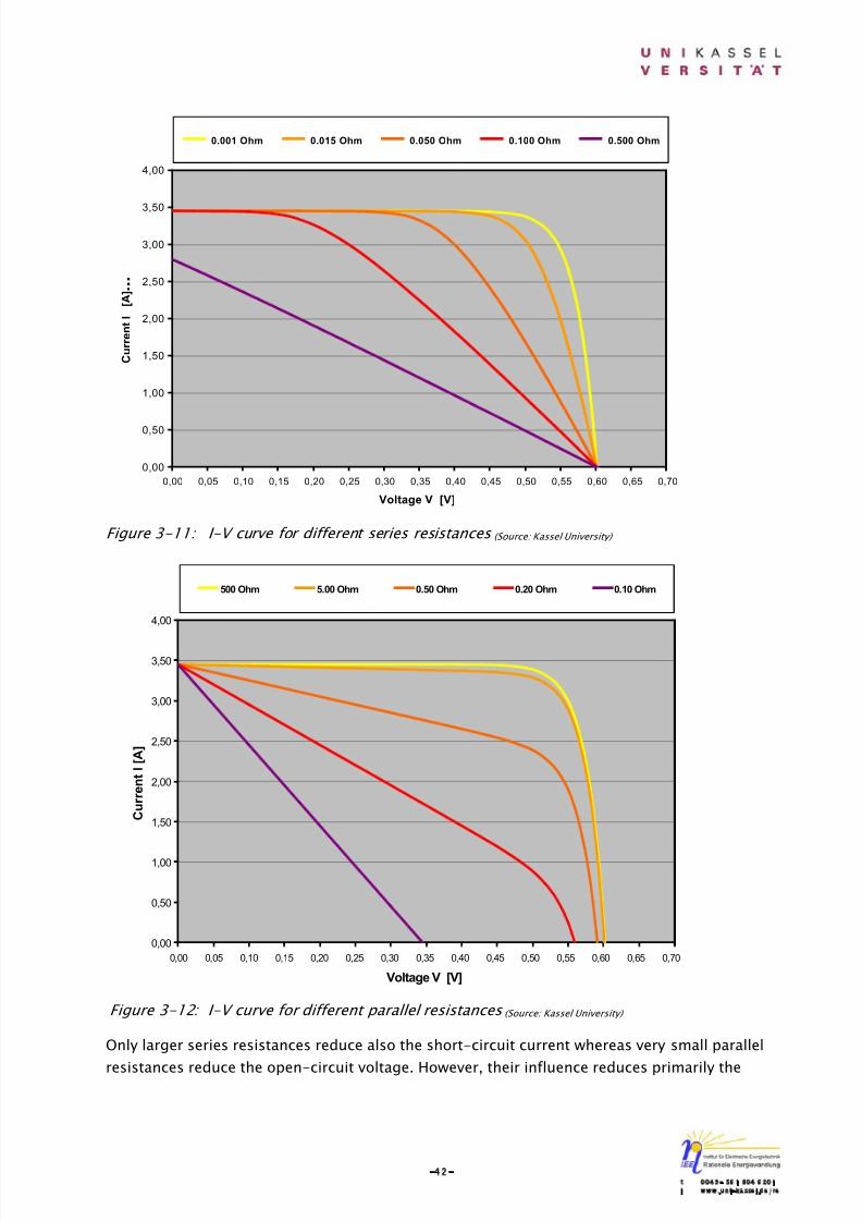
8/14/2019 Photovoltaic Systems Technology SS 2003
http://slidepdf.com/reader/full/photovoltaic-systems-technology-ss-2003 46/155
-42-t 0049- 561 804 6201i www.uni-kassel.de/re
Figure 3-11: I-V curve for different series resistances (Source: Kassel University)
Figure 3-12: I-V curve for different parallel resistances (Source: Kassel University)
Only larger series resistances reduce also the short-circuit current whereas very small parallel
resistances reduce the open-circuit voltage. However, their influence reduces primarily the
0,00
0,50
1,00
1,50
2,00
2,50
3,00
3,50
4,00
0,00 0,05 0,10 0,15 0,20 0,25 0,30 0,35 0,40 0,45 0,50 0,55 0,60 0,65 0,70
Voltage V [V]
C u r r e n t I [ A ] . . .
0.001 Ohm 0.015 Ohm 0.050 Ohm 0.100 Ohm 0.500 Ohm
0,00
0,50
1,00
1,50
2,00
2,50
3,00
3,50
4,00
0,00 0,05 0,10 0,15 0,20 0,25 0,30 0,35 0,40 0,45 0,50 0,55 0,60 0,65 0,70
Voltage V [V]
C u r r e n t I [ A ]
500 Ohm 5.00 Ohm 0.50 Ohm 0.20 Ohm 0.10 Ohm
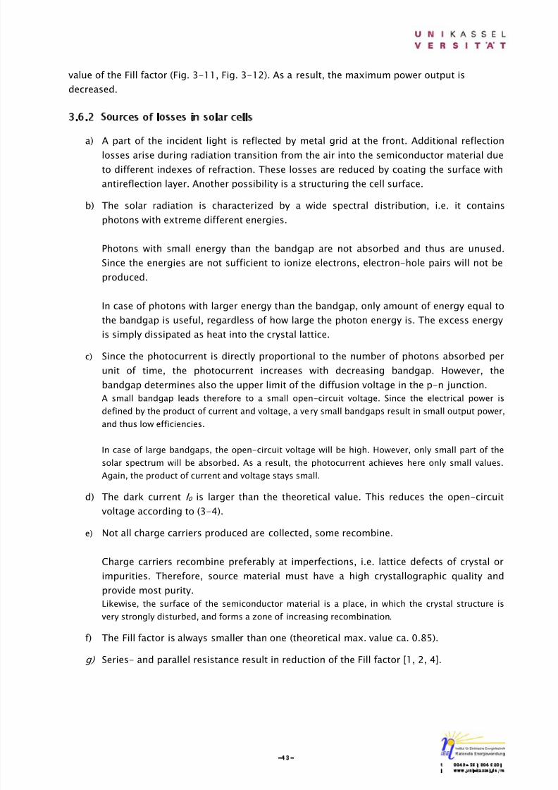
8/14/2019 Photovoltaic Systems Technology SS 2003
http://slidepdf.com/reader/full/photovoltaic-systems-technology-ss-2003 47/155
-43-t 0049- 561 804 6201i www.uni-kassel.de/re
value of the Fill factor (Fig. 3-11, Fig. 3-12). As a result, the maximum power output is
decreased.
3.6.2 Sources of losses in solar cells
a) A part of the incident light is reflected by metal grid at the front. Additional reflectionlosses arise during radiation transition from the air into the semiconductor material due
to different indexes of refraction. These losses are reduced by coating the surface with
antireflection layer. Another possibility is a structuring the cell surface.
b) The solar radiation is characterized by a wide spectral distribution, i.e. it contains
photons with extreme different energies.
Photons with small energy than the bandgap are not absorbed and thus are unused.
Since the energies are not sufficient to ionize electrons, electron-hole pairs will not be
produced.
In case of photons with larger energy than the bandgap, only amount of energy equal to
the bandgap is useful, regardless of how large the photon energy is. The excess energy
is simply dissipated as heat into the crystal lattice.
c) Since the photocurrent is directly proportional to the number of photons absorbed per
unit of time, the photocurrent increases with decreasing bandgap. However, the
bandgap determines also the upper limit of the diffusion voltage in the p-n junction.
A small bandgap leads therefore to a small open-circuit voltage. Since the electrical power is
defined by the product of current and voltage, a very small bandgaps result in small output power,and thus low efficiencies.
In case of large bandgaps, the open-circuit voltage will be high. However, only small part of the
solar spectrum will be absorbed. As a result, the photocurrent achieves here only small values.
Again, the product of current and voltage stays small.
d) The dark current I 0 is larger than the theoretical value. This reduces the open-circuit
voltage according to (3-4).
e) Not all charge carriers produced are collected, some recombine.
Charge carriers recombine preferably at imperfections, i.e. lattice defects of crystal or
impurities. Therefore, source material must have a high crystallographic quality and
provide most purity.
Likewise, the surface of the semiconductor material is a place, in which the crystal structure is
very strongly disturbed, and forms a zone of increasing recombination.
f) The Fill factor is always smaller than one (theoretical max. value ca. 0.85).
g) Series- and parallel resistance result in reduction of the Fill factor [1, 2, 4].
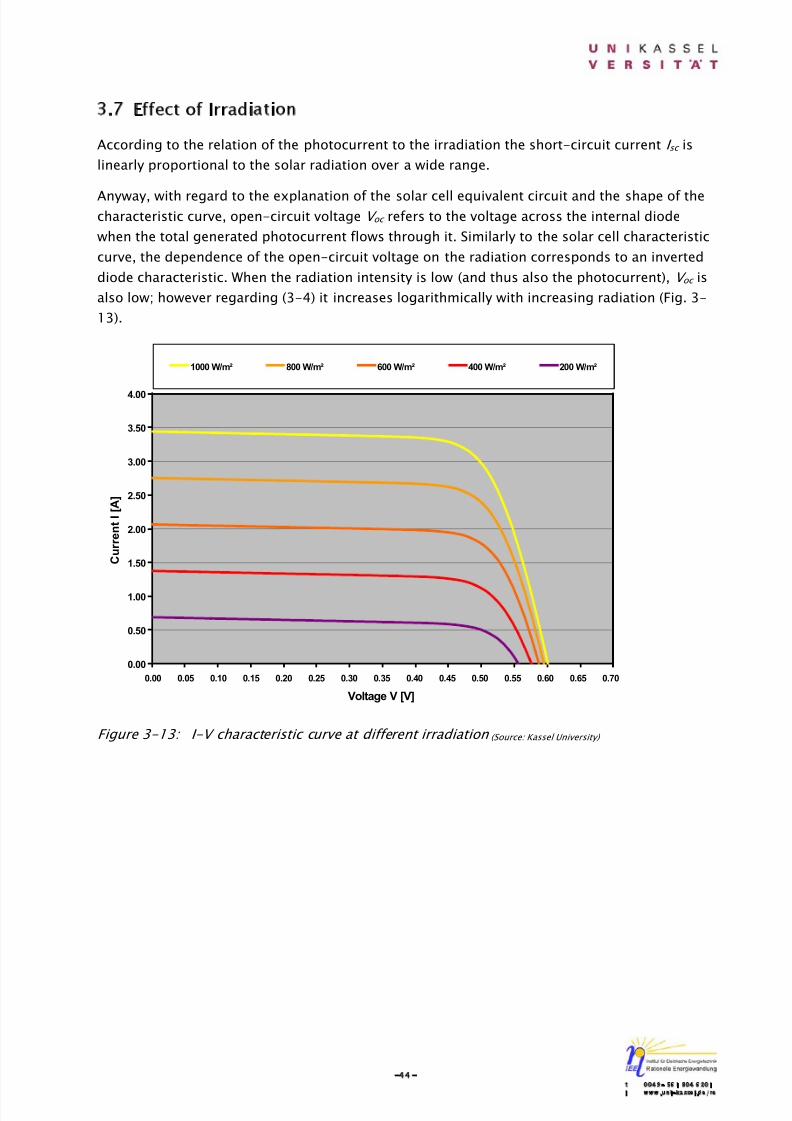
8/14/2019 Photovoltaic Systems Technology SS 2003
http://slidepdf.com/reader/full/photovoltaic-systems-technology-ss-2003 48/155
-44-t 0049- 561 804 6201i www.uni-kassel.de/re
3.7 Effect of Irradiation
According to the relation of the photocurrent to the irradiation the short-circuit current I sc is
linearly proportional to the solar radiation over a wide range.
Anyway, with regard to the explanation of the solar cell equivalent circuit and the shape of thecharacteristic curve, open-circuit voltage V oc refers to the voltage across the internal diode
when the total generated photocurrent flows through it. Similarly to the solar cell characteristic
curve, the dependence of the open-circuit voltage on the radiation corresponds to an inverted
diode characteristic. When the radiation intensity is low (and thus also the photocurrent), V oc is
also low; however regarding (3-4) it increases logarithmically with increasing radiation (Fig. 3-
13).
0.00
0.50
1.00
1.50
2.00
2.50
3.00
3.50
4.00
0.00 0.05 0.10 0.15 0.20 0.25 0.30 0.35 0.40 0.45 0.50 0.55 0.60 0.65 0.70
Voltage V [V]
C u r r e n t I [ A ]
1000 W/m² 800 W/m² 600 W/m² 400 W/m² 200 W/m²
Figure 3-13: I-V characteristic curve at different irradiation (Source: Kassel University)
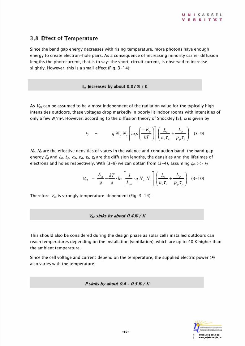
8/14/2019 Photovoltaic Systems Technology SS 2003
http://slidepdf.com/reader/full/photovoltaic-systems-technology-ss-2003 49/155
-45-t 0049- 561 804 6201i www.uni-kassel.de/re
3.8 Effect of Temperature
Since the band gap energy decreases with rising temperature, more photons have enough
energy to create electron-hole pairs. As a consequence of increasing minority carrier diffusion
lengths the photocurrent, that is to say: the short-circuit current, is observed to increaseslightly. However, this is a small effect (Fig. 3-14):
As V oc can be assumed to be almost independent of the radiation value for the typically high
intensities outdoors, these voltages drop markedly in poorly lit indoor rooms with intensities of
only a few W/m2. However, according to the diffusion theory of Shockley [5], I 0 is given by
I 0 =
+
−
p p
p
nn
n g
cv p
L
n
L
kT
E exp N N q
τ τ (3-9)
N v , N c are the effective densities of states in the valence and conduction band, the band gap
energy E g and L n , L p , n n , p p , τ n , τ p are the diffusion lengths, the densities and the lifetimes of
electrons and holes respectively. With (3-9) we can obtain from (3-4), assuming I ph >> I 0 :
V oc =
+
⋅⋅−
p p
p
nn
ncv
ph
g
p
L
n
L N N q
I
1 ln
q
kT
q
E
τ τ (3-10)
Therefore V oc is strongly temperature-dependent (Fig. 3-14):
This should also be considered during the design phase as solar cells installed outdoors can
reach temperatures depending on the installation (ventilation), which are up to 40 K higher thanthe ambient temperature.
Since the cell voltage and current depend on the temperature, the supplied electric power (P )
also varies with the temperature:
Isc increases by about 0.07 % / K
P sinks by about 0.4 – 0.5 % / K
Voc sinks by about 0.4 % / K
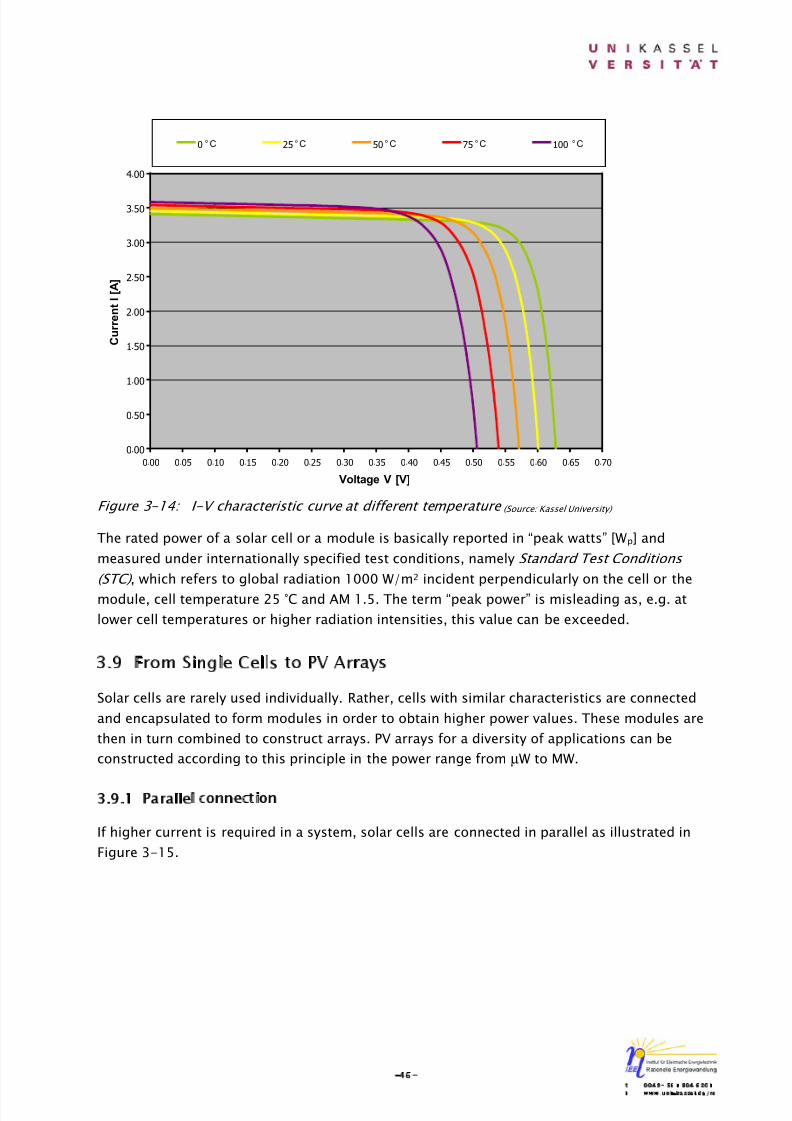
8/14/2019 Photovoltaic Systems Technology SS 2003
http://slidepdf.com/reader/full/photovoltaic-systems-technology-ss-2003 50/155
-46-t 0049- 561 804 6201i www.uni-kassel.de/re
Figure 3-14: I-V characteristic curve at different temperature (Source: Kassel University)
The rated power of a solar cell or a module is basically reported in “peak watts” [Wp] and
measured under internationally specified test conditions, namely Standard Test Conditions
(STC) , which refers to global radiation 1000 W/m2 incident perpendicularly on the cell or the
module, cell temperature 25 °C and AM 1.5. The term “peak power” is misleading as, e.g. at
lower cell temperatures or higher radiation intensities, this value can be exceeded.
3.9 From Single Cells to PV Arrays
Solar cells are rarely used individually. Rather, cells with similar characteristics are connected
and encapsulated to form modules in order to obtain higher power values. These modules are
then in turn combined to construct arrays. PV arrays for a diversity of applications can be
constructed according to this principle in the power range from µW to MW.
3.9.1 Parallel connection
If higher current is required in a system, solar cells are connected in parallel as illustrated in
Figure 3-15.
Solarzellen IU Kennlini
0.00
0.50
1.00
1.50
2.00
2.50
3.00
3.50
4.00
0.00 0.05 0.10 0.15 0.20 0.25 0.30 0.35 0.40 0.45 0.50 0.55 0.60 0.65 0.70
Voltage V [V]
C u r r e n t I [ A ]
0 °C 25 °C 50 °C 75 °C 100 °C
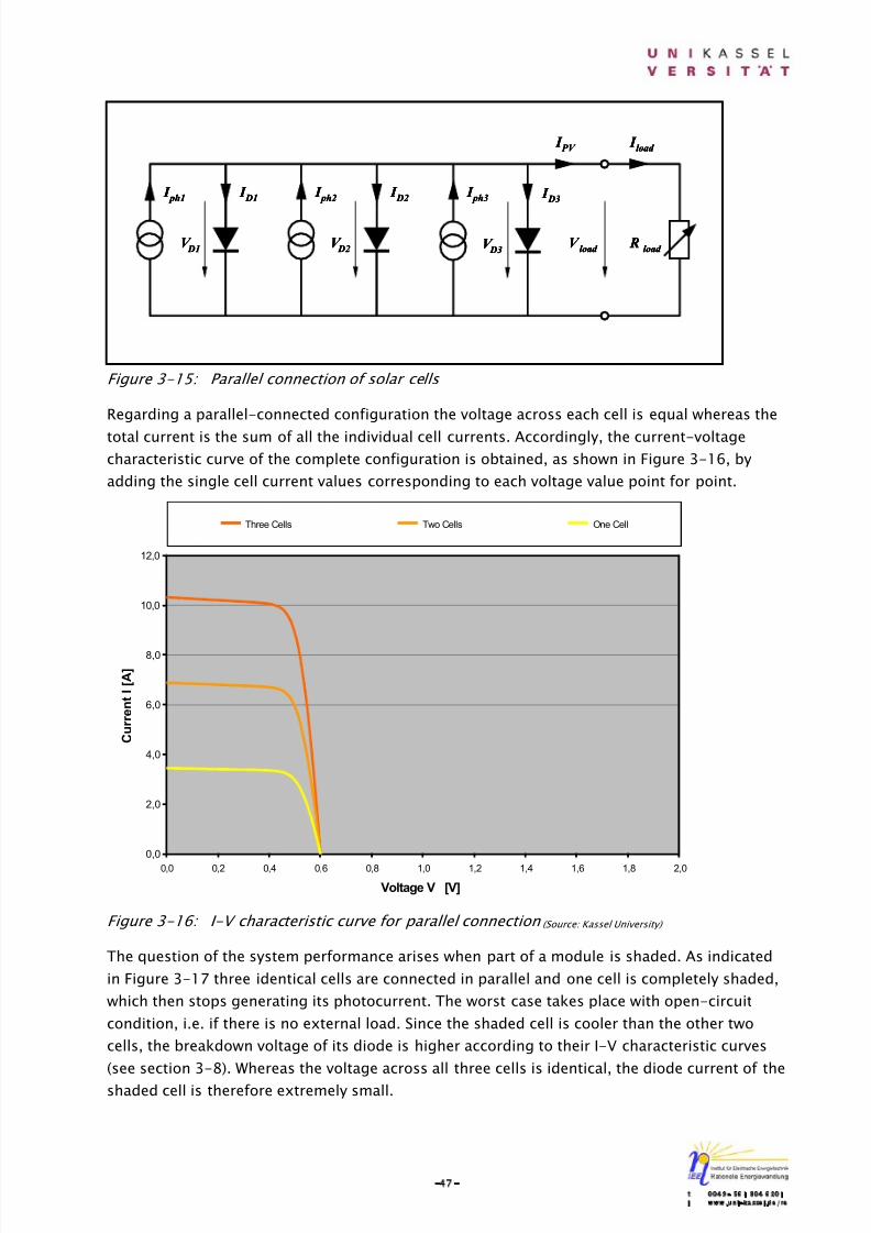
8/14/2019 Photovoltaic Systems Technology SS 2003
http://slidepdf.com/reader/full/photovoltaic-systems-technology-ss-2003 51/155
-47-t 0049- 561 804 6201i www.uni-kassel.de/re
Figure 3-15: Parallel connection of solar cells
Regarding a parallel-connected configuration the voltage across each cell is equal whereas the
total current is the sum of all the individual cell currents. Accordingly, the current-voltagecharacteristic curve of the complete configuration is obtained, as shown in Figure 3-16, by
adding the single cell current values corresponding to each voltage value point for point.
Figure 3-16: I-V characteristic curve for parallel connection (Source: Kassel University)
The question of the system performance arises when part of a module is shaded. As indicated
in Figure 3-17 three identical cells are connected in parallel and one cell is completely shaded,
which then stops generating its photocurrent. The worst case takes place with open-circuit
condition, i.e. if there is no external load. Since the shaded cell is cooler than the other two
cells, the breakdown voltage of its diode is higher according to their I-V characteristic curves
(see section 3-8). Whereas the voltage across all three cells is identical, the diode current of the
shaded cell is therefore extremely small.
I ph1
I load
I D1
V D1
V load
Rload
I PV
I ph2
I D2
V D2
I ph3 I
D3
V D3
I ph1
I ph1
I load
I load
I D1
I D1
V D1
V D1
V load
V load
Rload
Rload
I PV
I PV
I ph2
I ph2
I D2
I D2
V D2
V D2
I ph3
I ph3 I
D3 I
D3
V D3
V D3
0,0
2,0
4,0
6,0
8,0
10,0
12,0
0,0 0,2 0,4 0,6 0,8 1,0 1,2 1,4 1,6 1,8 2,0
Voltage V [V]
C u r r e n t I [ A ]
Three Cells Two Cells One Cell
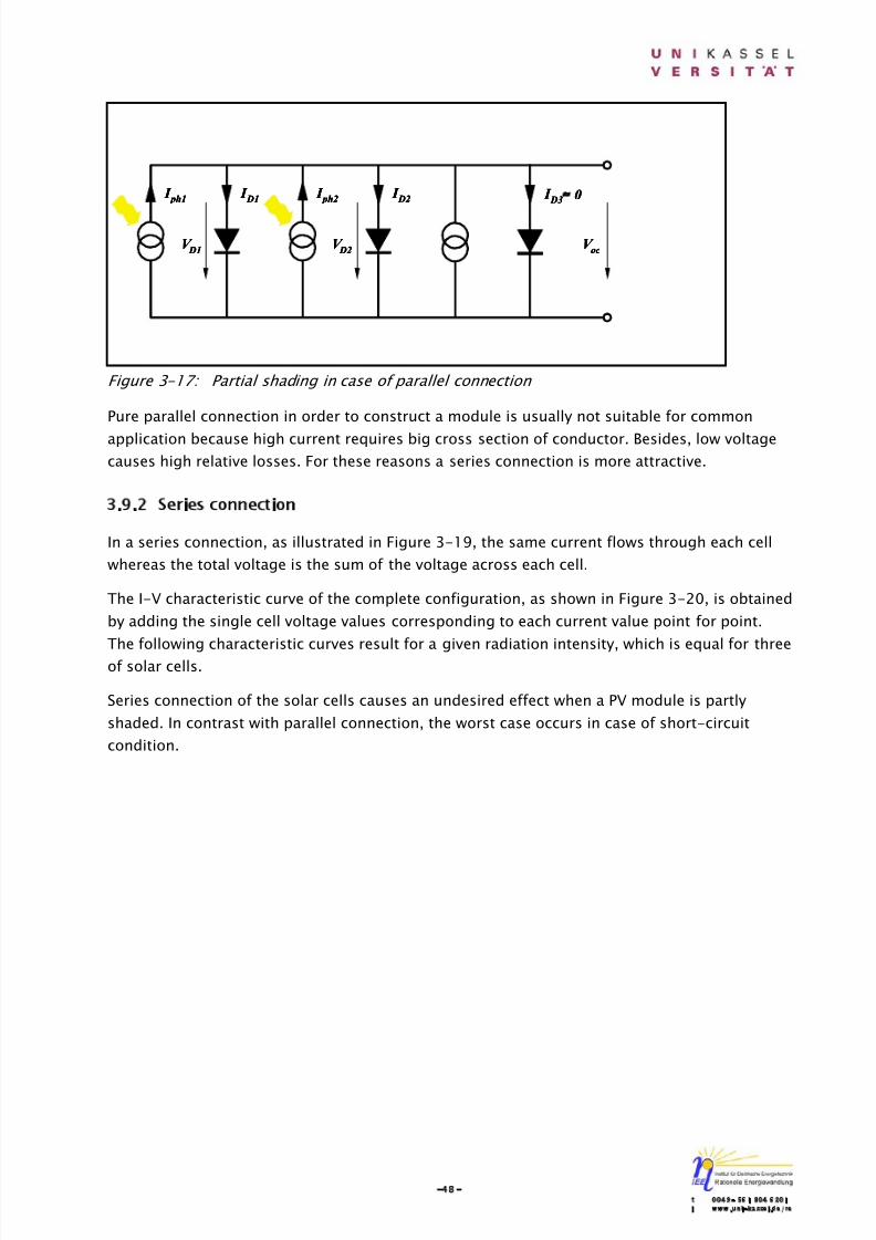
8/14/2019 Photovoltaic Systems Technology SS 2003
http://slidepdf.com/reader/full/photovoltaic-systems-technology-ss-2003 52/155
-48-t 0049- 561 804 6201i www.uni-kassel.de/re
Figure 3-17: Partial shading in case of parallel connection
Pure parallel connection in order to construct a module is usually not suitable for common
application because high current requires big cross section of conductor. Besides, low voltagecauses high relative losses. For these reasons a series connection is more attractive.
3.9.2 Series connection
In a series connection, as illustrated in Figure 3-19, the same current flows through each cell
whereas the total voltage is the sum of the voltage across each cell.
The I-V characteristic curve of the complete configuration, as shown in Figure 3-20, is obtained
by adding the single cell voltage values corresponding to each current value point for point.
The following characteristic curves result for a given radiation intensity, which is equal for threeof solar cells.
Series connection of the solar cells causes an undesired effect when a PV module is partly
shaded. In contrast with parallel connection, the worst case occurs in case of short-circuit
condition.
I ph1
I D1
V D1
I ph2
I D2
V D2
V oc
I D3≈ 0 I
ph1 I
ph1 I
D1 I
D1
V D1
V D1
I ph2
I ph2
I D2
I D2
V D2
V D2
V oc
V oc
I D3≈ 0 I D3≈ 0
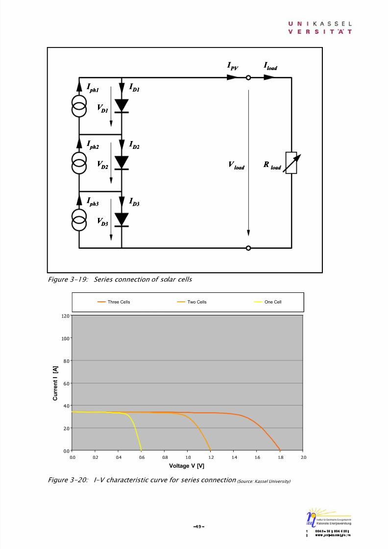
8/14/2019 Photovoltaic Systems Technology SS 2003
http://slidepdf.com/reader/full/photovoltaic-systems-technology-ss-2003 53/155
-49-t 0049- 561 804 6201i www.uni-kassel.de/re
Figure 3-19: Series connection of solar cells
Figure 3-20: I-V characteristic curve for series connection (Source: Kassel University)
I ph3
V D3
Rload
I PV
V D2
V D1
I ph1
I ph2
I D1
I D3
I D2
I load
V load
I ph3
I ph3
V D3
V D3
Rload
Rload
I PV
I PV
V D2
V D2
V D1
V D1
I ph1
I ph1
I ph2
I ph2
I D1
I D1
I D3
I D3
I D2
I D2
I load
I load
V load
V load
0.0
2.0
4.0
6.0
8.0
10.0
12.0
0.0 0.2 0.4 0.6 0.8 1.0 1.2 1.4 1.6 1.8 2.0
Voltage V [V]
C u r r e n
t I [ A ]
Three Cells Two Cells One Cell
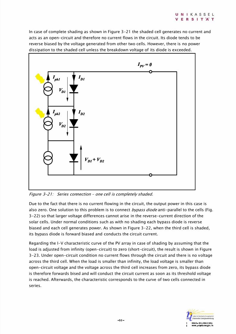
8/14/2019 Photovoltaic Systems Technology SS 2003
http://slidepdf.com/reader/full/photovoltaic-systems-technology-ss-2003 54/155
-50-t 0049- 561 804 6201i www.uni-kassel.de/re
In case of complete shading as shown in Figure 3-21 the shaded cell generates no current and
acts as an open-circuit and therefore no current flows in the circuit. Its diode tends to be
reverse biased by the voltage generated from other two cells. However, there is no power
dissipation to the shaded cell unless the breakdown voltage of its diode is exceeded.
Figure 3-21: Series connection – one cell is completely shaded.
Due to the fact that there is no current flowing in the circuit, the output power in this case is
also zero. One solution to this problem is to connect bypass diode anti-parallel to the cells (Fig.
3-22) so that larger voltage differences cannot arise in the reverse-current direction of the
solar cells. Under normal conditions such as with no shading each bypass diode is reverse
biased and each cell generates power. As shown in Figure 3-22, when the third cell is shaded,
its bypass diode is forward biased and conducts the circuit current.
Regarding the I-V characteristic curve of the PV array in case of shading by assuming that the
load is adjusted from infinity (open-circuit) to zero (short-circuit), the result is shown in Figure
3-23. Under open-circuit condition no current flows through the circuit and there is no voltage
across the third cell. When the load is smaller than infinity, the load voltage is smaller than
open-circuit voltage and the voltage across the third cell increases from zero, its bypass diode
is therefore forwards bised and will conduct the circuit current as soon as its threshold voltage
is reached. Afterwards, the characteristic corresponds to the curve of two cells connected in
series.
V D2
V D1
I ph1
I ph2
I D1
I D2
V D1 + V D2
I PV = 0
V D2
V D2
V D1
V D1
I ph1
I ph1
I ph2
I ph2
I D1
I D1
I D2
I D2
V D1 + V D2V D1 + V D2
I PV = 0 I PV = 0

8/14/2019 Photovoltaic Systems Technology SS 2003
http://slidepdf.com/reader/full/photovoltaic-systems-technology-ss-2003 55/155
-51-t 0049- 561 804 6201i www.uni-kassel.de/re
Figure 3-22: Series connection with bypass diodes – one cell is completely shaded.
Figure 3-23: I-V characteristic curve for series connection – one cell is completely shaded
V D2
V D1
I ph1
I ph2
I D1
I D2
Bypass
Diode
Bypass
Diode
Bypass
Diode
I cell 1 = I cell 2
V D2
V D2
V D1
V D1
I ph1
I ph1
I ph2
I ph2
I D1
I D1
I D2
I D2
Bypass
Diode
Bypass
Diode
Bypass
Diode
Bypass
Diode
Bypass
Diode
Bypass
Diode
I cell 1 = I cell 2 I cell 1 = I cell 2
0,0
2,0
4,0
6,0
8,0
10,0
12,0
0,0 0,2 0,4 0,6 0,8 1,0 1,2 1,4 1,6 1,8 2,0
Voltage V .[V]
C u r r e n t I . [ A ]
Three Cells Two Cells One Cell Shading with bypass
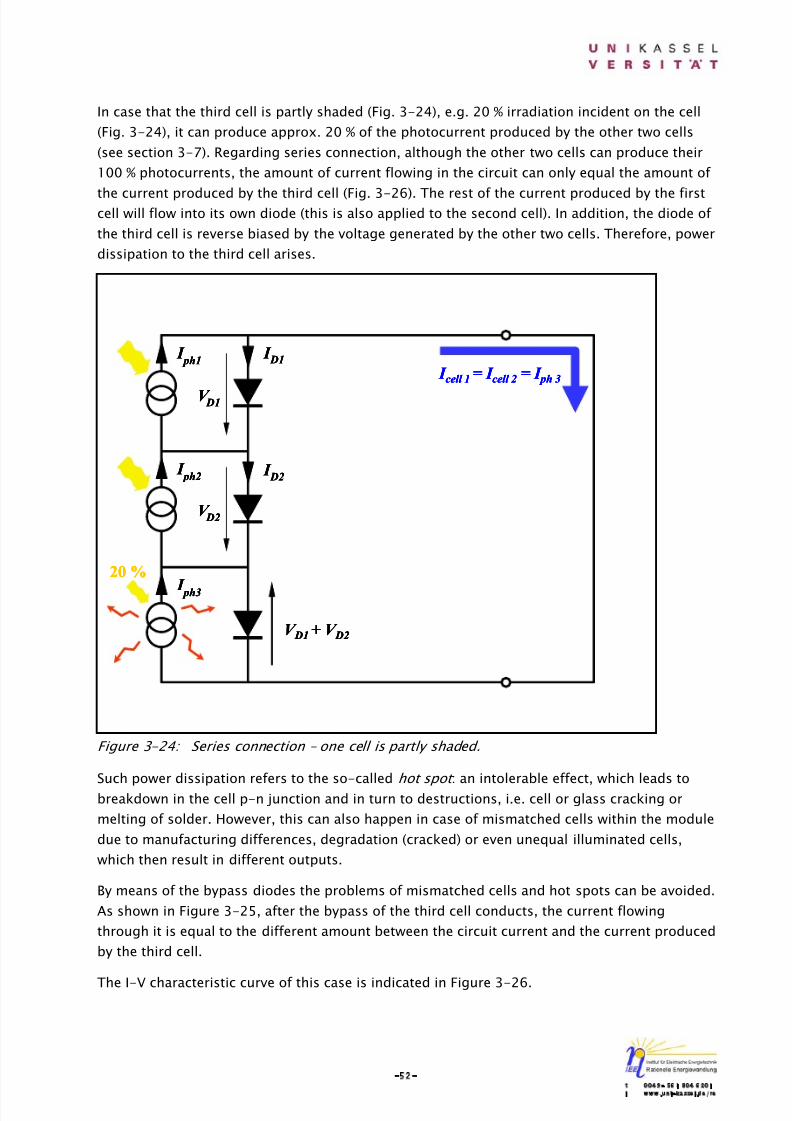
8/14/2019 Photovoltaic Systems Technology SS 2003
http://slidepdf.com/reader/full/photovoltaic-systems-technology-ss-2003 56/155
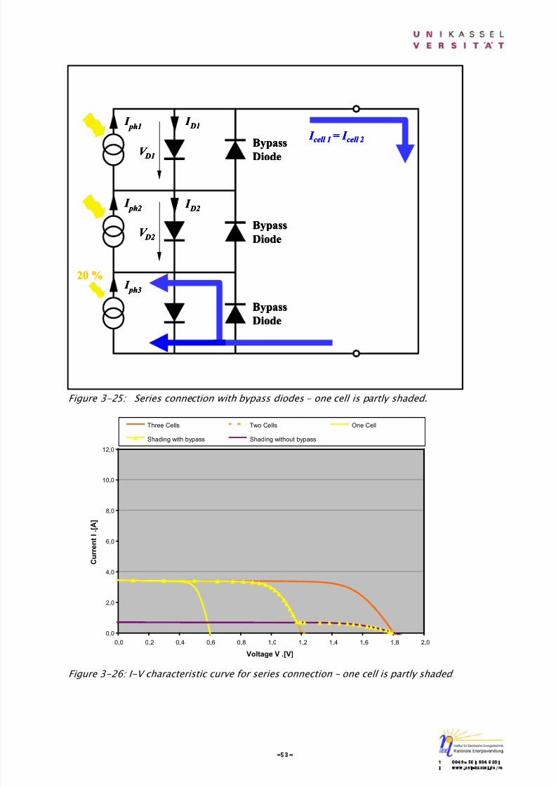
8/14/2019 Photovoltaic Systems Technology SS 2003
http://slidepdf.com/reader/full/photovoltaic-systems-technology-ss-2003 57/155
-53-t 0049- 561 804 6201i www.uni-kassel.de/re
Figure 3-25: Series connection with bypass diodes – one cell is partly shaded.
Figure 3-26: I-V characteristic curve for series connection – one cell is partly shaded
V D2
V D1
I ph1
I ph2
I ph3
20 %
I D1
I D2
Bypass
Diode
Bypass
Diode
Bypass
Diode
I cell 1 = I cell 2
V D2V D2
V D1
V D1
I ph1
I ph1
I ph2
I ph2
I ph3
I ph3
20 %20 %
I D1
I D1
I D2
I D2
Bypass
Diode
Bypass
Diode
Bypass
Diode
Bypass
Diode
Bypass
Diode
Bypass
Diode
I cell 1 = I cell 2 I cell 1 = I cell 2
0,0
2,0
4,0
6,0
8,0
10,0
12,0
0,0 0,2 0,4 0,6 0,8 1,0 1,2 1,4 1,6 1,8 2,0
Voltage V .[V]
C u r r
e n t I . [ A
]
Three Cells Two Cells One Cell
Shading with bypass Shading without bypass
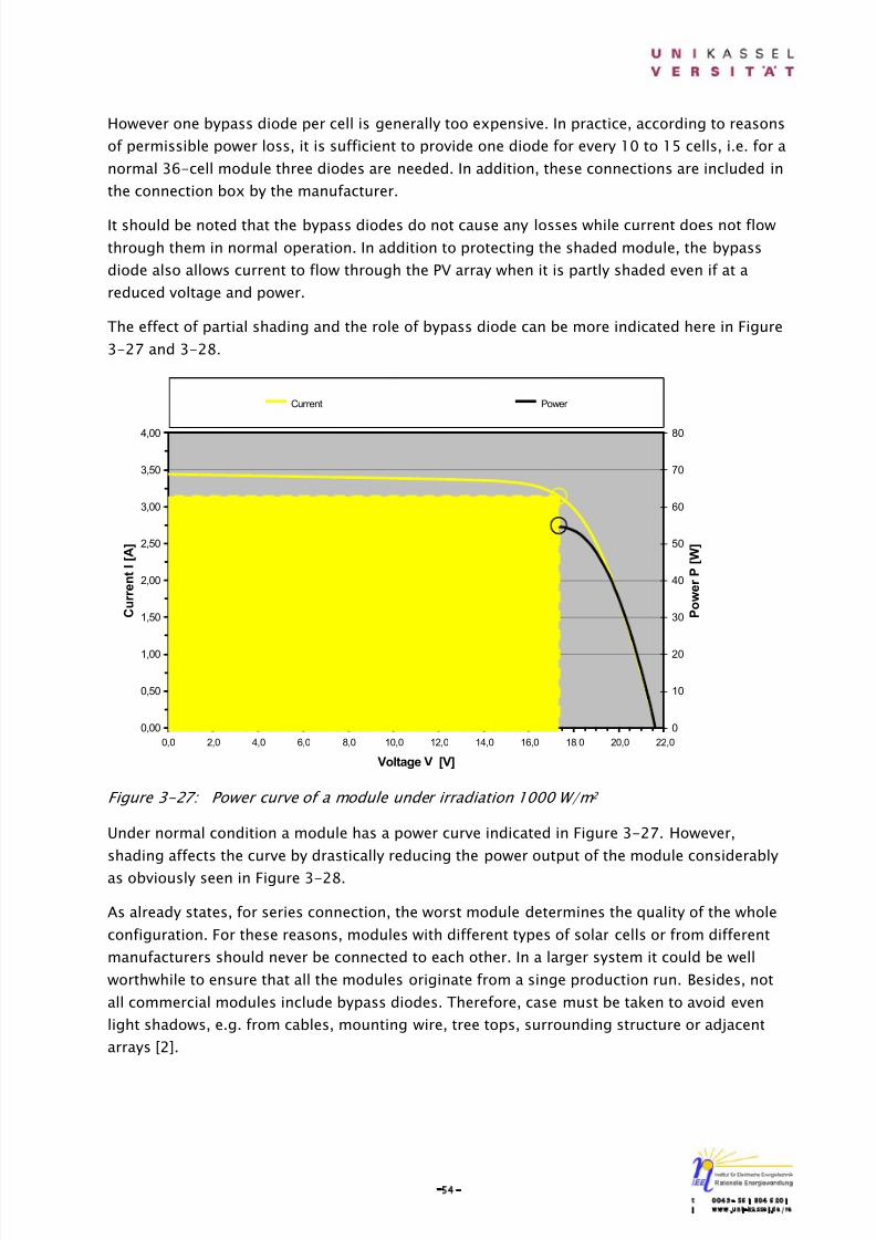
8/14/2019 Photovoltaic Systems Technology SS 2003
http://slidepdf.com/reader/full/photovoltaic-systems-technology-ss-2003 58/155
-54-t 0049- 561 804 6201i www.uni-kassel.de/re
However one bypass diode per cell is generally too expensive. In practice, according to reasons
of permissible power loss, it is sufficient to provide one diode for every 10 to 15 cells, i.e. for a
normal 36-cell module three diodes are needed. In addition, these connections are included in
the connection box by the manufacturer.
It should be noted that the bypass diodes do not cause any losses while current does not flow
through them in normal operation. In addition to protecting the shaded module, the bypass
diode also allows current to flow through the PV array when it is partly shaded even if at a
reduced voltage and power.
The effect of partial shading and the role of bypass diode can be more indicated here in Figure
3-27 and 3-28.
Figure 3-27: Power curve of a module under irradiation 1000 W/m 2
Under normal condition a module has a power curve indicated in Figure 3-27. However,
shading affects the curve by drastically reducing the power output of the module considerably
as obviously seen in Figure 3-28.
As already states, for series connection, the worst module determines the quality of the whole
configuration. For these reasons, modules with different types of solar cells or from different
manufacturers should never be connected to each other. In a larger system it could be well
worthwhile to ensure that all the modules originate from a singe production run. Besides, not
all commercial modules include bypass diodes. Therefore, case must be taken to avoid even
light shadows, e.g. from cables, mounting wire, tree tops, surrounding structure or adjacent
arrays [2].
0,00
0,50
1,00
1,50
2,00
2,50
3,00
3,50
4,00
0,0 2,0 4,0 6,0 8,0 10,0 12,0 14,0 16,0 18,0 20,0 22,0
Voltage V [V]
C u r r e n t I [ A ]
0
10
20
30
40
50
60
70
80
P o w e r P [ W ]
Current Power
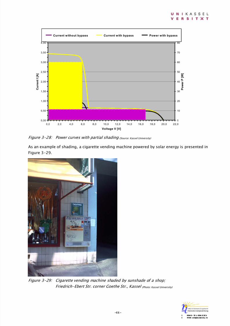
8/14/2019 Photovoltaic Systems Technology SS 2003
http://slidepdf.com/reader/full/photovoltaic-systems-technology-ss-2003 59/155

8/14/2019 Photovoltaic Systems Technology SS 2003
http://slidepdf.com/reader/full/photovoltaic-systems-technology-ss-2003 60/155
-56-t 0049- 561 804 6201i www.uni-kassel.de/re
According to Figure 3-29, with an unsuitable mounting the PV module installed on the top of
the machine stays under shadow of the shop’s sunshade during the day. Furthermore, the PV
module faces dirt as well (Fig. 3-30). However, this module is little over-dimensioned according
to a small different of prices and the machine needs only small power for its required function.
Figure 3-30: PV module of the cigarette vending machine (Photo: Kassel University)
Another example of shading, which takes place often with PV modules, is due to birds’
droppings when they settle on the upper edge of the module (Fig. 3-31). A solution in order to
prevent settling of birds, a strip of needles can be mounted along the upper edge of themodule.
Figure 3-31: Dirt on the PV module due to birds’ droppings supply for a glass showcase
at Karlsplatz, Kassel (Photo: Kassel University)
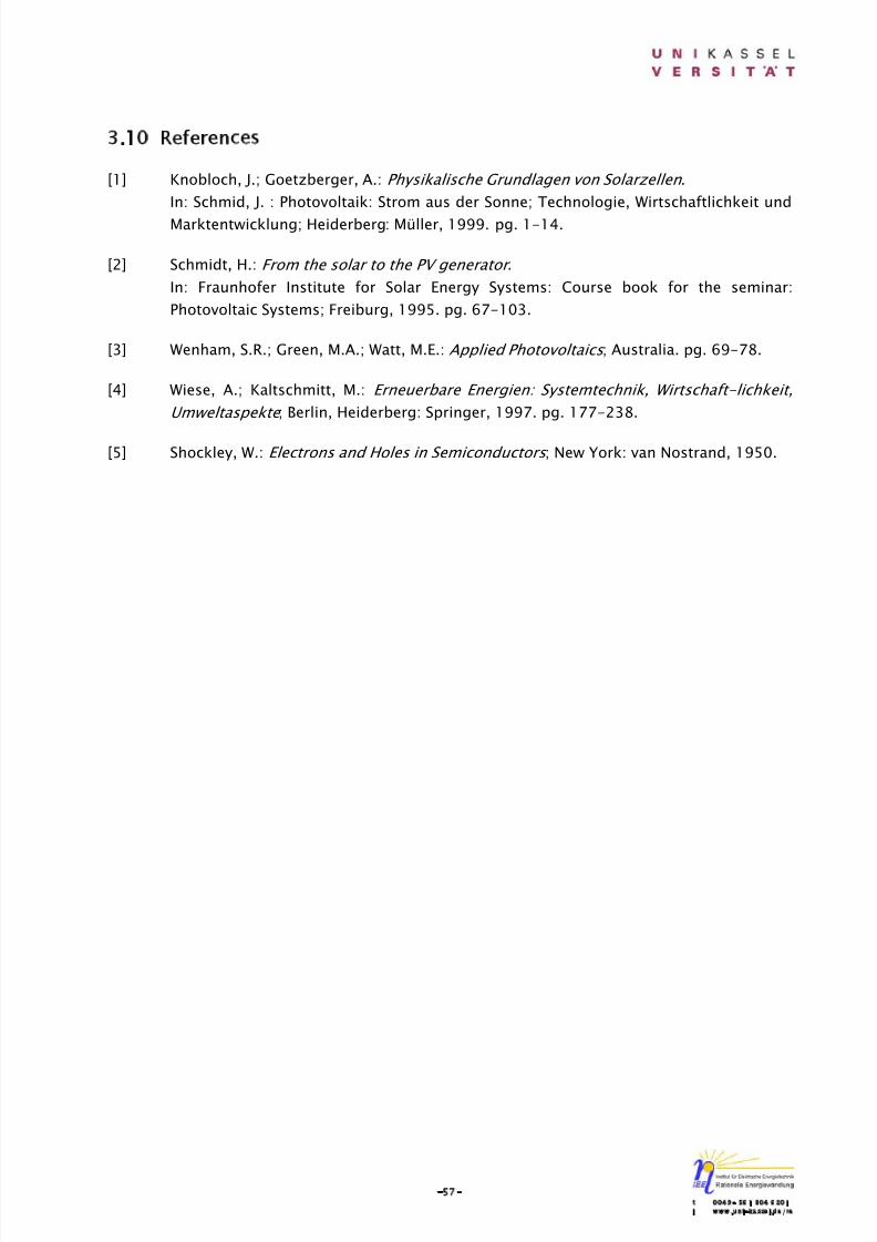
8/14/2019 Photovoltaic Systems Technology SS 2003
http://slidepdf.com/reader/full/photovoltaic-systems-technology-ss-2003 61/155
-57-t 0049- 561 804 6201i www.uni-kassel.de/re
3.10 References
[1] Knobloch, J.; Goetzberger, A.: Physikalische Grundlagen von Solarzellen .
In: Schmid, J. : Photovoltaik: Strom aus der Sonne; Technologie, Wirtschaftlichkeit und
Marktentwicklung; Heiderberg: Müller, 1999. pg. 1-14.
[2] Schmidt, H.: From the solar to the PV generator .
In: Fraunhofer Institute for Solar Energy Systems: Course book for the seminar:
Photovoltaic Systems; Freiburg, 1995. pg. 67-103.
[3] Wenham, S.R.; Green, M.A.; Watt, M.E.: Applied Photovoltaics ; Australia. pg. 69-78.
[4] Wiese, A.; Kaltschmitt, M.: Erneuerbare Energien: Systemtechnik, Wirtschaft-lichkeit,
Umweltaspekte ; Berlin, Heiderberg: Springer, 1997. pg. 177-238.
[5] Shockley, W.: Electrons and Holes in Semiconductors ; New York: van Nostrand, 1950.

8/14/2019 Photovoltaic Systems Technology SS 2003
http://slidepdf.com/reader/full/photovoltaic-systems-technology-ss-2003 62/155
-58-t 0049- 561 804 6201i www.uni-kassel.de/re
4 CONVERSION PRINCIPLES IN PV SYSTEMS
4.1 Introduction
PV generator is a heart of a PV system. For a practical application, however, additional
components are needed, e.g. for the energy storage, for the energy flow regulation or for the
supply of network-conformal alternating voltages and currents. These additional components
represent a considerable share of cost, efficiency reduction and influence the behavior of the
whole system substantially.
Assuming the representation of a solar cell by a current source parallel with a diode its
standard symbol is illustrated in Figure 4-1.
Figure 4-1: Symbol of a PV generator
4.2 Coupling of PV Generator and Ohmic Load
In case that loads are directly connected to linear sources, electric power (voltages and
currents) are supplied to the load. The values of voltage and current for each operating point
can be easily calculated with the help of Ohm’s Law if e.g. a voltage source is connected to a
resistor. However, if the source has a non linear nature, e.g. in case of PV generators (Fig. 4-2),
a graphical method is necessary.
I D
I PV
V PV
I PV
V PV V D
I ph
I D
I D
I PV
I PV
V PV V PV
I PV
I PV
V PV V PV V DV D
I ph
I ph
8/14/2019 Photovoltaic Systems Technology SS 2003
http://slidepdf.com/reader/full/photovoltaic-systems-technology-ss-2003 63/155
-59-t 0049- 561 804 6201i www.uni-kassel.de/re
Figure 4-2: Direct coupling of PV generator and ohmic load
The characteristic curves of both, the PV generator and the resistive load, are overlaid on the
same graphic. The PV genaretor is a source whereas the resistence is a load. The two
components are connected to each other, the voltage is equal across both and the same current
flows through the whole circuit, therefore the intersection of the two characteristic curves is the
resulting working point, as shown in Figure 4-3 [1].
Figure 4-3: Working points for different irradiations (Source: Kassel University)
Assuming that operating temperature of solar cells is constant; I-V curves of a PV generator fordifferent irradiations are represented for different load curves in Figure 4-3. The load curve II
V load
I PV
V PV
PV
Generator
I load
Rload
V load
V load
I PV I PV
V PV
V PV
PV
Generator
I load I load
Rload
Rload
0,00
0,50
1,00
1,50
2,00
2,50
3,00
3,50
4,00
0,0 2,0 4,0 6,0 8,0 10,0 12,0 14,0 16,0 18,0 20,0 22,0
Voltage V [V]
C u r r e n t I [ A ]
1000 W/m² 600 W/m² 200 W/m² Load I Load II
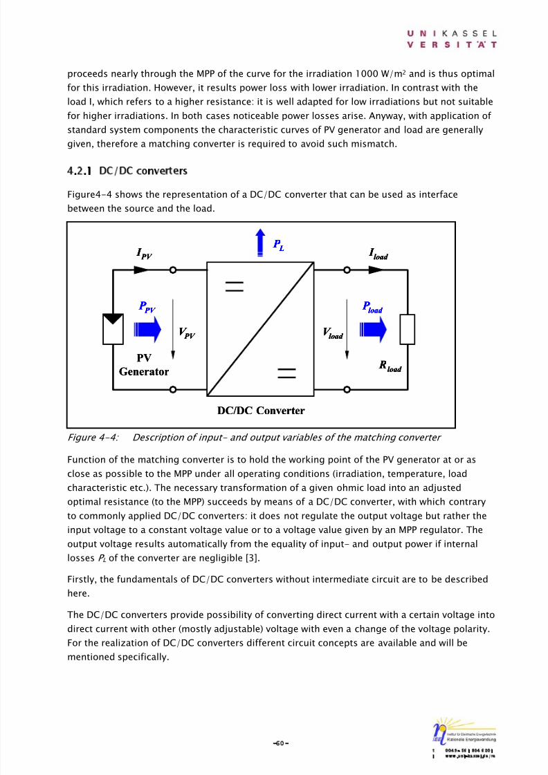
8/14/2019 Photovoltaic Systems Technology SS 2003
http://slidepdf.com/reader/full/photovoltaic-systems-technology-ss-2003 64/155
-60-t 0049- 561 804 6201i www.uni-kassel.de/re
proceeds nearly through the MPP of the curve for the irradiation 1000 W/m2 and is thus optimal
for this irradiation. However, it results power loss with lower irradiation. In contrast with the
load I, which refers to a higher resistance: it is well adapted for low irradiations but not suitable
for higher irradiations. In both cases noticeable power losses arise. Anyway, with application of
standard system components the characteristic curves of PV generator and load are generally
given, therefore a matching converter is required to avoid such mismatch.
4.2.1 DC/DC converters
Figure4-4 shows the representation of a DC/DC converter that can be used as interface
between the source and the load.
Figure 4-4: Description of input- and output variables of the matching converter
Function of the matching converter is to hold the working point of the PV generator at or as
close as possible to the MPP under all operating conditions (irradiation, temperature, load
characteristic etc.). The necessary transformation of a given ohmic load into an adjusted
optimal resistance (to the MPP) succeeds by means of a DC/DC converter, with which contrary
to commonly applied DC/DC converters: it does not regulate the output voltage but rather the
input voltage to a constant voltage value or to a voltage value given by an MPP regulator. The
output voltage results automatically from the equality of input- and output power if internallosses P L of the converter are negligible [3].
Firstly, the fundamentals of DC/DC converters without intermediate circuit are to be described
here.
The DC/DC converters provide possibility of converting direct current with a certain voltage into
direct current with other (mostly adjustable) voltage with even a change of the voltage polarity.
For the realization of DC/DC converters different circuit concepts are available and will be
mentioned specifically.
V load
I PV
V PV
DC/DC Converter
I load
Rload
P load
P PV
PV
Generator
P L
V load
V load
I PV
I PV
V PV
V PV
DC/DC Converter
I load
I load
Rload
Rload
P load
P load
P PV
P PV
PV
Generator
P L
P L
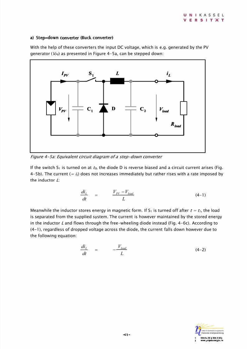
8/14/2019 Photovoltaic Systems Technology SS 2003
http://slidepdf.com/reader/full/photovoltaic-systems-technology-ss-2003 65/155

8/14/2019 Photovoltaic Systems Technology SS 2003
http://slidepdf.com/reader/full/photovoltaic-systems-technology-ss-2003 66/155
-62-t 0049- 561 804 6201i www.uni-kassel.de/re
Figure 4-5b: Step-down converter during “on” state
Figure 4-5c: Step-down converter during “off” state
The capacitor C1 is used to support the supply voltage (V PV ). In principle, S1 is turned on and off
with a switching frequency (that is to say: with “t on ” and “t off ”). With regard to Ohm’s law the
behaviour of the load voltage can be obtained from the load current (= i L ). As shown in Fig. 4-
5d, the resulted load voltage has obviously a ripple, which can be smoothed by additional
capacitor C2. Anyway, its average value (V load ) is lower than V PV . In case that the switching
frequency is increased, e.g. up to the kHz-range, then the necessary inductance can be reduced
considerably.
D
L i L
V PV
S1
C2C1 V load D
L i Li L
V PV V PV
S1
S1
C2C2C1C1 V load V load
D
L i L
I PV
V PV
S1
C2
C1 V
load D
L i Li L
I PV
I PV
V PV
V PV
S1
S1
C2
C2
C1
C1 V
load V
load
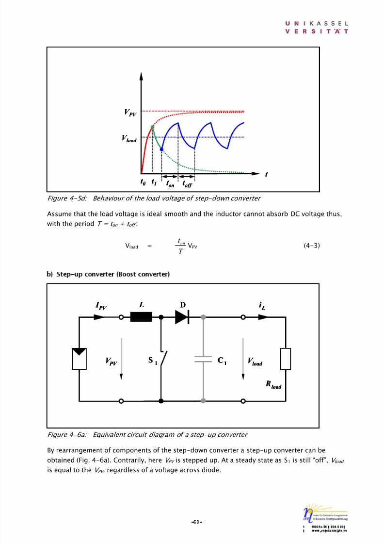
8/14/2019 Photovoltaic Systems Technology SS 2003
http://slidepdf.com/reader/full/photovoltaic-systems-technology-ss-2003 67/155
-63-t 0049- 561 804 6201i www.uni-kassel.de/re
Figure 4-5d: Behaviour of the load voltage of step-down converter
Assume that the load voltage is ideal smooth and the inductor cannot absorb DC voltage thus,
with the period T = t on + t off :
Vload =T
t on VPV (4-3)
b) Step-up converter (Boost converter)
Figure 4-6a: Equivalent circuit diagram of a step-up converter
By rearrangement of components of the step-down converter a step-up converter can be
obtained (Fig. 4-6a). Contrarily, here V PV is stepped up. At a steady state as S1 is still “off”, V load
is equal to the V PV , regardless of a voltage across diode.
V PV
t t on t off
t 1t 0
V load
V PV
t t on t off
t 1t 0
V load
I PV
V PV
Rload
C1
L i L
S1
D
V load
I PV
I PV
V PV
V PV
Rload Rload
C1
C1
L i Li L
S1
S1
D
V load
V load

8/14/2019 Photovoltaic Systems Technology SS 2003
http://slidepdf.com/reader/full/photovoltaic-systems-technology-ss-2003 68/155
-64-t 0049- 561 804 6201i www.uni-kassel.de/re
Figure 4-6b: Step-up converter during “on” state
As shown in Figure 4-6b, during “on” state, without C1 the load voltage drops immediately to
zero. The circuit current (= i L ) flows through the inductor L and S1 and rises according to the
following equatsion:
dt
di L = L
V PV (4-4)
Figure 4-6c: Step-up converter during “off” state
After S1 is switched off (Fig. 4-6c), the induced voltage in the inductor adds itself to V PV , which
lie then across the load. i L flows through the inductor and further to the load. Thereby it falls
down gradually because V load > V PV :
dt
di L = L
V V load PV − (4-5)
L i L
S1
D
C1 V
load
I PV
V PV
L i Li L
S1
S1
D
C1
C1 V
load V
load
I PV
I PV
V PV
V PV
Rload
L
i L
S1
D
C1 V
load
I PV
V PV
Rload
Rload
L
i Li L
S1
S1
D
C1
C1 V
load V
load
I PV I PV
V PV
V PV

8/14/2019 Photovoltaic Systems Technology SS 2003
http://slidepdf.com/reader/full/photovoltaic-systems-technology-ss-2003 69/155
-65-t 0049- 561 804 6201i www.uni-kassel.de/re
Figure 4-6d: Behaviour of the load voltage of step-up converter
The proceeding of the load voltage is illustrated in Figure 4-6d. The diode D protects against a
short circuit (that is to say: discharge) of the charged capacitor C1, which is assumed to be so
big that it can smooth the load voltage completely:
Vload = PV
off
V t
T (4-6)
c) Step-down/Step-up converter (Buck/Boost or inverting converter)
This circuit (Fig. 4-7a) enables both step-down and step-up of a DC voltage. During the “on”
state the energy given by the source (PV generator, in this case) is stored in the inductor L (Fig.
4-7b). The stored energy in the inductor L is delivered then to R load during the “off” state (Fig.
4-7c). With the help of the diode D the current flows through the inductor L only in one
direction during both “on”- and “off” state. As a result, V load has obviously an opposite polarity
to V PV . Therefore, the circuit is also called inverting converter . Equations describing the
proceeding of the circuit currents can be derived in the same way to both converters mentioned
before and will not be done here. As stated, the capacitor C1 supports the supply voltage V PV
and C2 smoothes V load . In conclusion the amplitude of V load can be either lower or higher thanV PV depending on the adjusted t on and consequently t off [8]:
V load = − t
t
off
on V PV (4-7)
V PV
t t on t off
t 0
V load
V PV
t t on t off
t 0
V load
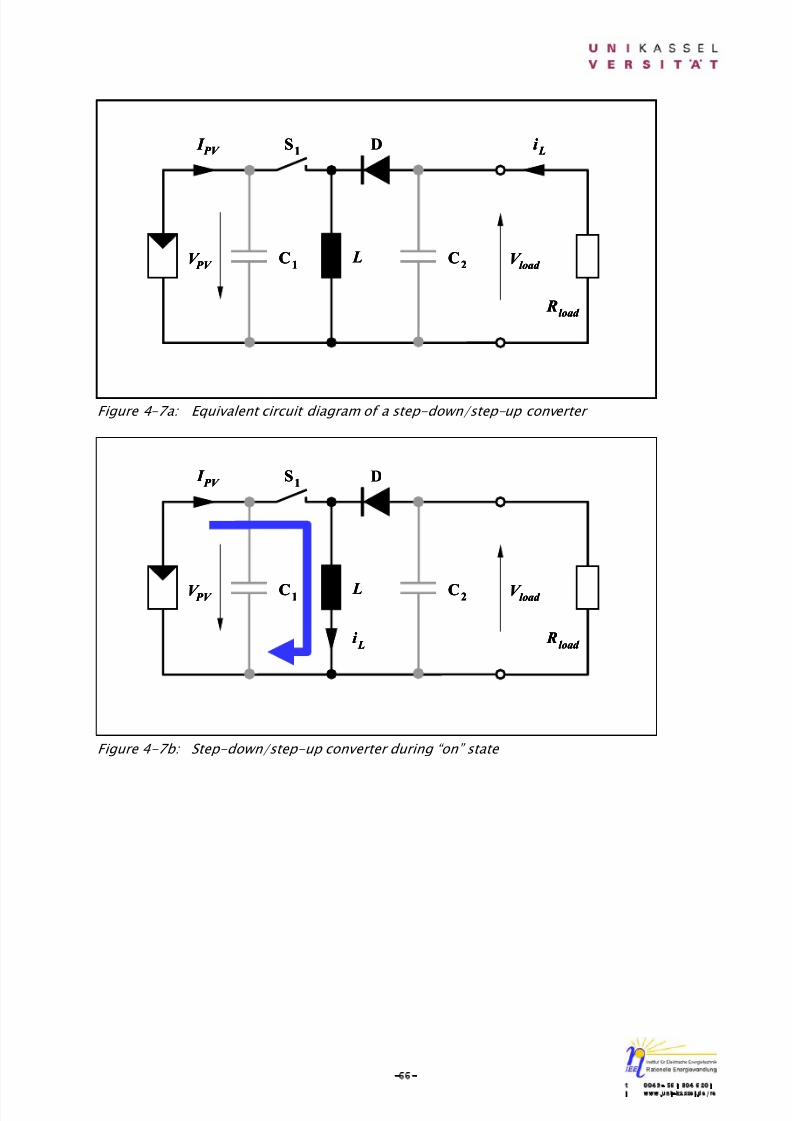
8/14/2019 Photovoltaic Systems Technology SS 2003
http://slidepdf.com/reader/full/photovoltaic-systems-technology-ss-2003 70/155
-66-t 0049- 561 804 6201i www.uni-kassel.de/re
Figure 4-7a: Equivalent circuit diagram of a step-down/step-up converter
Figure 4-7b: Step-down/step-up converter during “on” state
I PV
V PV L
Rload
D i L
C2
C1
S1
V load
I PV I PV
V PV V PV L
Rload
Rload
D i Li L
C2
C2
C1
C1
S1S1
V load V load
I PV
V PV L
Rload
D
i L
C2C1
S1
V load
I PV
I PV
V PV V PV L
Rload
Rload
D
i Li L
C2C2C1C1
S1
S1
V load V load
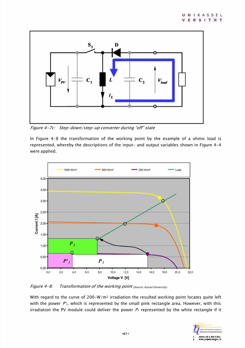
8/14/2019 Photovoltaic Systems Technology SS 2003
http://slidepdf.com/reader/full/photovoltaic-systems-technology-ss-2003 71/155
-67-t 0049- 561 804 6201i www.uni-kassel.de/re
Figure 4-7c: Step-down/step-up converter during “off” state
In Figure 4-8 the transformation of the working point by the example of a ohmic load is
represented, whereby the descriptions of the input- and output variables shown in Figure 4-4
were applied.
Figure 4-8: Transformation of the working point (Source: Kassel University)
With regard to the curve of 200-W/m2 irradiation the resulted working point locates quite left
with the power P ′ 1, which is represented by the small pink rectangle area. However, with thisirradiation the PV module could deliver the power P 1 represented by the white rectangle if it
V PV
L V load
D
i L
C2
C1
S1
V PV
V PV
L V load
V load
D
i Li L
C2
C2
C1
C1
S1
S1
0,00
0,50
1,00
1,50
2,00
2,50
3,00
3,50
4,00
0,0 2,0 4,0 6,0 8,0 10,0 12,0 14,0 16,0 18,0 20,0 22,0
Voltage V [V]
C u r r e n t I [ A ]
1000 W/m² 600 W/m² 200 W/m² Load
P 1
P 2
P' 1
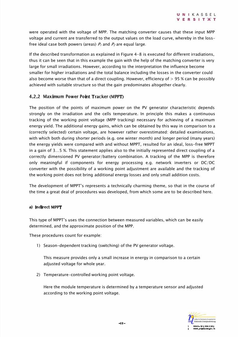
8/14/2019 Photovoltaic Systems Technology SS 2003
http://slidepdf.com/reader/full/photovoltaic-systems-technology-ss-2003 72/155
8/14/2019 Photovoltaic Systems Technology SS 2003
http://slidepdf.com/reader/full/photovoltaic-systems-technology-ss-2003 73/155
-69-t 0049- 561 804 6201i www.uni-kassel.de/re
3) Measurement of the PV generator’s open circuit voltage.
This method is based on the fact that for a certain module the relationship between
open circuit voltage and MPP voltage can be approximated by a constant factor of e.g.
0.8 or also a simple function. With this procedure the open circuit voltage is measured
within regular intervals by short separation of the load and then the desired working
point voltage is determined.
The advantage of the procedures mentioned can be a very simple feasibility - it is however
disadvantageous that in general only an approximation to the actual MPP is achieved and
modifications of the PV generator characteristic, e.g. by contamination, cannot be taken into
account.
b) Direct MPPT
This MPPT’s get the information about the desired optimal working point from actuallymeasured currents, voltages or powers in the system and thus can react also to unforeseeable
modifications in the behavior of the PV generator.
Usually assigned procedures are based on a search algorithm, with which the maximum of the
power curve is determined without interruption of the normal operation. For this, in regular
intervals, the working point voltage is changed around a certain increment - consequently
output power becomes larger, then the search direction is maintained for the next step,
otherwise it is reverse. The actual working point oscillates therefore with a certain range around
the actual point of maximum power. This simple basic principle can be secured by additional
algorithms against misinterpretations, which can occur for example with a wrong searchdirection and nevertheless a rising power due to fast increasing irradiation.
The necessary determination for searching the MPP of the PV generator power requires in
principle a measurement of generator voltage and current as well as a multiplication of these
variables. A substantial simplification results, if one considers that the actual target is not a
maximization of generator output power, but rather achieving a maximum power at the load. It
is therefore meaningful and simpler to detect and maximize either the voltage at the load or
usually the current through the load [3].
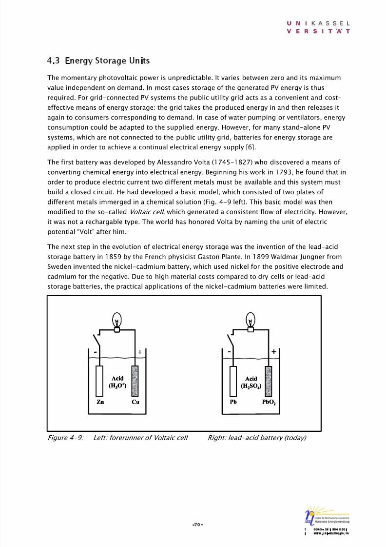
8/14/2019 Photovoltaic Systems Technology SS 2003
http://slidepdf.com/reader/full/photovoltaic-systems-technology-ss-2003 74/155
-70-t 0049- 561 804 6201i www.uni-kassel.de/re
4.3 Energy Storage Units
The momentary photovoltaic power is unpredictable. It varies between zero and its maximum
value independent on demand. In most cases storage of the generated PV energy is thus
required. For grid-connected PV systems the public utility grid acts as a convenient and cost-effective means of energy storage: the grid takes the produced energy in and then releases it
again to consumers corresponding to demand. In case of water pumping or ventilators, energy
consumption could be adapted to the supplied energy. However, for many stand-alone PV
systems, which are not connected to the public utility grid, batteries for energy storage are
applied in order to achieve a continual electrical energy supply [6].
The first battery was developed by Alessandro Volta (1745-1827) who discovered a means of
converting chemical energy into electrical energy. Beginning his work in 1793, he found that in
order to produce electric current two different metals must be available and this system must
build a closed circuit. He had developed a basic model, which consisted of two plates of different metals immerged in a chemical solution (Fig. 4-9 left). This basic model was then
modified to the so-called Voltaic cell , which generated a consistent flow of electricity. However,
it was not a rechargable type. The world has honored Volta by naming the unit of electric
potential “Volt” after him.
The next step in the evolution of electrical energy storage was the invention of the lead-acid
storage battery in 1859 by the French physicist Gaston Plante. In 1899 Waldmar Jungner from
Sweden invented the nickel-cadmium battery, which used nickel for the positive electrode and
cadmium for the negative. Due to high material costs compared to dry cells or lead-acid
storage batteries, the practical applications of the nickel-cadmium batteries were limited.
Figure 4-9: Left: forerunner of Voltaic cell Right: lead-acid battery (today)
-
Zn Cu
Acid
(H3O+)
+ - +
Acid
(H2SO4)
Pb PbO2
--
ZnZn CuCu
Acid
(H3O+)
Acid
(H3O+)
++ -- ++
Acid
(H2SO4)
Acid
(H2SO4)
PbPb PbO2PbO2
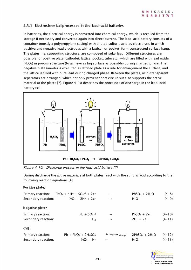
8/14/2019 Photovoltaic Systems Technology SS 2003
http://slidepdf.com/reader/full/photovoltaic-systems-technology-ss-2003 75/155
-71-t 0049- 561 804 6201i www.uni-kassel.de/re
4.3.1 Electrochemical processes in the lead-acid batteries
In batteries, the electrical energy is converted into chemical energy, which is recalled from the
storage if necessary and converted again into direct current. The lead-acid battery consists of a
container (mostly a polypropylene casing) with diluted sulfuric acid as electrolyte, in which
positive and negative lead electrodes with a lattice- or pocket-form constructed surface hang.
The plates, i.e. supporting structure, are composed of solar lead. Different structures are
possible for positive plate (cathode): lattice, pocket, tube etc., which are filled with lead oxide
(PbO2) in porous structure (to achieve as big surface as possible) during charged phase. The
negative plate (anode) is executed as latticed plate as a rule for enlargement the surface, and
the lattice is filled with pure lead during charged phase. Between the plates, acid-transparent
separators are arranged, which not only prevent short circuit but also supports the active
material at the plates [7]. Figure 4-10 describes the processes of discharge in the lead-acid
battery cell.
Figure 4-10: Discharge process in the lead-acid battery [7]
During discharge the active materials at both plates react with the sulfuric acid according to the
following reaction equations [4]:
Positive plate:Primary reaction: PbO2 + 4H+ + SO4
-2 + 2e- → PbSO4 + 2H2O (4-8)
Secondary reaction: ½O2 + 2H+ + 2e- → H2O (4-9)
Negative plate:
Primary reaction: Pb + SO4-2 → PbSO4 + 2e- (4-10)
Secondary reaction: H2 → 2H+ + 2e- (4-11)
Cell:
Primary reaction: Pb + PbO2 + 2H2SO4 discharge charge 2PbSO4 + 2H2O (4-12)
Secondary reaction: ½O2 + H2 → H2O (4-13)
-
Pb
Pb + 2H2SO4 + PbO2 → 2PbSO4 + 2H2O
PbO2
H2SO4
+ - + - +
convert
to
PbSO4PbSO4
Plate
surface
converted
--
PbPb
Pb + 2H2SO4 + PbO2 → 2PbSO4 + 2H2O
PbO2PbO2
H2SO4H2SO4
++ -- ++ -- ++
convert
to
convert
to
PbSO4PbSO4PbSO4PbSO4
Plate
surface
converted
Plate
surface
converted

8/14/2019 Photovoltaic Systems Technology SS 2003
http://slidepdf.com/reader/full/photovoltaic-systems-technology-ss-2003 76/155
-72-t 0049- 561 804 6201i www.uni-kassel.de/re
At the positive plate a part of lead oxide (PbO2) reacts with a part of the sulfuric acid (SO4-ion)
to produce a part of lead sulphate (PbSO4) whereas at the negative plate a part of lead reacts
with a part of acid to produce a part of lead sulphate and 2 parts of water (Fig. 4-11). Since
with the discharge reaction acid is reduced and water is produced, the acid concentration in the
cell drops with increasing discharge.
Figure 4-11: Discharge process in the lead-acid battery
Figure 4-12: Charging process in the lead-acid battery [7]
By the way, regarding the equation (4-12), charging process with electric current supply
provides a reversal of the reaction (Fig. 4-12), i.e. the lead sulphate at the plates is converted to
sulfuric acid and lead or lead oxide, whereby the acid concentration increases [7].
-
Pb PbO2
H2SO4
+ - + -
+
convert
to
PbO2Pb
Plate
surface
PbSO4 PbSO4
Source
-
+
+
Source
-+
Source
-
Pb + 2H2SO4 + PbO2 ← 2PbSO4 + 2H2O
--
PbPb PbO2PbO2
H2SO4H2SO4
++ -- ++ --
++
convert
to
convert
to
PbO2PbO2PbPb
Plate
surface
Plate
surface
PbSO4PbSO4 PbSO4PbSO4
SourceSource
--
++
++
SourceSource
--++
SourceSource
--
Pb + 2H2SO4 + PbO2 ← 2PbSO4 + 2H2O
DiffusionPb
2H2O
H2SO
4
2e-
2H+
PbSO4
2H+
2e-
PbO2
Anode
H2SO
4
Cathode
PbSO4
H2SO
4H
2SO
4
DiffusionPbPb
2H2O2H
2O
H2SO
4H
2SO
4
2e-
2H+
PbSO4
PbSO4
2H+
2e-
PbO2
PbO2
Anode
H2SO
4H
2SO
4
Cathode
PbSO4
PbSO4
H2SO
4H
2SO
4H
2SO
4H
2SO
4
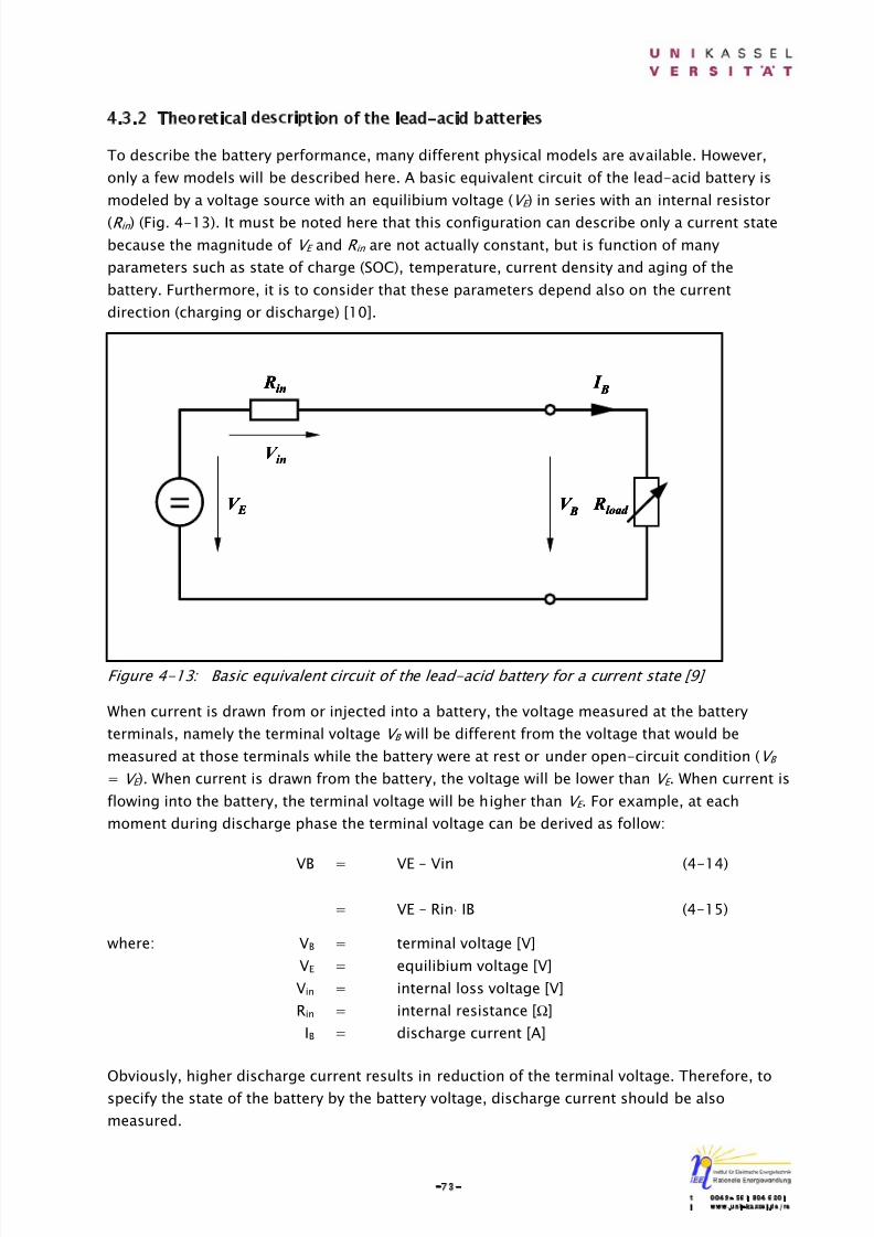
8/14/2019 Photovoltaic Systems Technology SS 2003
http://slidepdf.com/reader/full/photovoltaic-systems-technology-ss-2003 77/155
-73-t 0049- 561 804 6201i www.uni-kassel.de/re
4.3.2 Theoretical description of the lead-acid batteries
To describe the battery performance, many different physical models are available. However,
only a few models will be described here. A basic equivalent circuit of the lead-acid battery is
modeled by a voltage source with an equilibium voltage (V E ) in series with an internal resistor
(R in ) (Fig. 4-13). It must be noted here that this configuration can describe only a current state
because the magnitude of V E and R in are not actually constant, but is function of many
parameters such as state of charge (SOC), temperature, current density and aging of the
battery. Furthermore, it is to consider that these parameters depend also on the current
direction (charging or discharge) [10].
Figure 4-13: Basic equivalent circuit of the lead-acid battery for a current state [9]
When current is drawn from or injected into a battery, the voltage measured at the battery
terminals, namely the terminal voltage V B will be different from the voltage that would be
measured at those terminals while the battery were at rest or under open-circuit condition (V B
= V E ). When current is drawn from the battery, the voltage will be lower than V E . When current is
flowing into the battery, the terminal voltage will be higher than V E . For example, at each
moment during discharge phase the terminal voltage can be derived as follow:
VB = VE – Vin (4-14)
= VE – Rin⋅ IB (4-15)
where: VB = terminal voltage [V]
VE = equilibium voltage [V]
Vin = internal loss voltage [V]
Rin = internal resistance [Ω]
IB = discharge current [A]
Obviously, higher discharge current results in reduction of the terminal voltage. Therefore, tospecify the state of the battery by the battery voltage, discharge current should be also
measured.
V B
V in
I B Rin
V E Rload V B
V B
V in
I B
I B Rin Rin
V E V E Rload Rload

8/14/2019 Photovoltaic Systems Technology SS 2003
http://slidepdf.com/reader/full/photovoltaic-systems-technology-ss-2003 78/155
-74-t 0049- 561 804 6201i www.uni-kassel.de/re
Figure 4-14 illustrates current-voltage characteristics and working points of a battery, which is
directly connected to 2 different ohmic loads by assuming that SOC and temperator of the
battery are constant. A distance between the green line and dash line corresponds to V in .
Figure 4-14: Working points of the battery for different ohmic loads (Source: Kassel University)
In PV systems it is necessary to know the performance of the batteries for longer period.Additional elements are therefore considered to explain a dynamic- and a quasi-static
processes (Fig. 4-15).
Regarding the dynamic processes overvoltages partly due to the chemical reaction and any
processes such as diffusion processes of ions in the electrolyte are simplified summarized and
are described as a polarization voltage (V p ) whereas a voltage drop in the grid and in the
electrolyte is represented by a resistance R Ω .
For the quasi-static processes, a capacitor C p , which is connected in parallel to a resistor R p ,
disappears. This derived model corresponds to the Shepherd model [10, 11], which is perhaps
the most spread model worldwide [12].
0,0
0,5
1,0
1,5
2,0
2,5
3,0
3,5
4,0
0,0 2,0 4,0 6,0 8,0 10,0 12,0 14,0 16,0 18,0 20,0 22,0
Voltage V [V]
C
u r r e n t I [ A ]
High SOC Medium SOC Low SOC Load I Load II
V in

8/14/2019 Photovoltaic Systems Technology SS 2003
http://slidepdf.com/reader/full/photovoltaic-systems-technology-ss-2003 79/155
-75-t 0049- 561 804 6201i www.uni-kassel.de/re
Figure 4-15: Equivalent circuit of the battery regarding the dynamic- and
quasi-static processes [11]
An additional loss in the battery is due to self-discharge, which is represented by a resistor R S
(Fig. 4-15). This resistance is responsible for the emptiness of charged batteries after they are
left for so long although they are never in use. Good solar batteries should therefore have very
high R S in order to keep this loss as small as possible.
IB = I - IS (4-16)
where: I = battery current, which should be provided [A]IS = self-discharge current [A]
Anyway, the rated voltage of the lead-acid battery cell amounts of 2 V. A common 12-V battery
consists therefore of 6 series connected cells. In practical, the terminal voltage varies according
to operating condition. However, due to the fact that acid concentration changes during
charging and discharge as stated before, the equilibrium voltage can be estimated with
following empirical equations:
VE ≈ Vk + acid concentration [g/cm3] (4-17)
where: V E = equilibrium voltage [V]
V k = 0.84…0.88 (dependent on battery types [4])
For example, regarding a battery with H2SO4 concentration 1.28 g/cm3 and V k = 0.84 for Tudor
batteries [9]: thus the equilibium ≈ 0.84 + 1.28 = 2.12 V.
However, long settling time caused by long diffusion time of sulfuric acid is problematic.
Therefore, the battery should be in neutral situation while the acid concentration is measured
[9].
In case of discharge, the minimum voltage level acceptable for a lead-acid battery is defined asdischarge voltage threshold . Falling below this threshold is called deep discharge , with which
R S
I S
I
V B
I B
Rload V E
V p
R p
RΩC p
R S
I S I S
I I
V BV B
I B
I B
Rload Rload V E V E
V p
R p R p
RΩ RΩC pC p
8/14/2019 Photovoltaic Systems Technology SS 2003
http://slidepdf.com/reader/full/photovoltaic-systems-technology-ss-2003 80/155
-76-t 0049- 561 804 6201i www.uni-kassel.de/re
the battery may suffer damage. In case that the battery is left longer after deep discharge, lead
of the support structure is converted to lead sulphate in rough-crystalline form, which during
charging can be only bad or cannot be converted again anymore. As a result, the battery loses a
part of its storage capacity; besides loss of support structure arises as well.
In practice, harmful deep discharge is to be prevented: the consumers will be compulsorydisconnected from battery as soon as the discharge voltage threshold is reached i.e. with the
help of a so-called deep discharge protection (DDP) (Fig. 4-31). This threshold is basically
given in the data sheets by the manufacturer for different discharge currents. Preferably, the
value of this threshold should depend on the discharge current. The relation between the
discharge current and the voltage during discharge for the lead-acid battery is presented in
Figure 4-16 [6].
Figure 4-16: Discharge characteristic curves (Source: HAGEN)
However in PV systems, which are typically characterized by very slow discharges, this threshold
may be conveniently set at approx. 1.95 V per cell or 11.7 V for 12-V battery [1]. Anyway, if the
battery is deep-discharged, it must be recharged immediately.
In order to charge the battery, i.e. to move the sulphate ions from the plates back into the
electrolyte, a voltage higher than the rated voltage must be applied. Consequently, the charge
voltage is situated between 2.0 – 2.4 V per cell or 12 – 14.4 V for 12-V battery. It increasesaccording to rising charges in the battery.
4.3.3 Gassing
With 2.3 – 2.4 V, namely the so-called gassing voltage , gas is developed at the electrodes in the
battery, by which the water is decomposed into hydrogen and oxygen. Both gases mix together
in the battery providing detonating gas (explosive!) and escape through ventilation opening in
the vent plug. With the gassing the battery loses also water, which must be refilled according to
maintenance within regular intervals. The gas is the unwelcome secondary reaction of the
chemical conversion during charging because current is consumed for the electrolysis andtherefore the storage efficiency of the battery is made worse unnecessarily.
8/14/2019 Photovoltaic Systems Technology SS 2003
http://slidepdf.com/reader/full/photovoltaic-systems-technology-ss-2003 81/155
-77-t 0049- 561 804 6201i www.uni-kassel.de/re
After the gassing voltage is exceeded, voltage stays approximately constant. The whole
charging current during this period results in H2 and O2, which is defined as loss. For this
reason, gassing can be represented by a zenor diode in series with a resistor R G (Fig. 4-17).
Figure 4-17: Quasi-static equivalent circuit with representation of gassing [12]
The zenor diode is reverse biased and therefore does not conduct until the charging voltage
exceeds its breakdown voltage, namely the gassing voltage. Then it functions as a voltage
regulator by keeping the voltage across it constant and allows the whole charging current to
pass through, which is dissipated in R G as heat. It must be noted that this concept can be
applied only for lead-acid batteries because gassing destroys gel batteries (sealed type of lead-acid batteries).
Continually, heavy gassing damages the battery, so that in the data sheet the manufacturers
give the so-called maximum charge voltage , which is not allowed to be exceeded during
charging. This voltage is situated about 2.3 – 2.4 V per cell (with 20 °C) corresponding to 13.8 –
14.4 V for 6 cells. In many battery types, small gassing for a short time is however required to
mix the electrolyte and to provide an equal acid concentration for whole cell volume [7].
Nowadays, a great deal of batteries is available on the market. Most of them are starter
batteries. The difference between solar- and starter batteries will be described as follow:
In the electrolyte, ions next to the surface of electrodes can provide immediately chemical
reaction resulting in a potential difference and contribute to current flow. Figure 4-18 shows a
comparison of porous structures of electrodes’ surfaces in solar batteries and in starter
batteries.
R S
I S
V B
RG
V G
I PV
V E
V in
Rin
R S
I S I S
V BV B
RG
V G
I PV I PV
V E V E
V in
Rin Rin
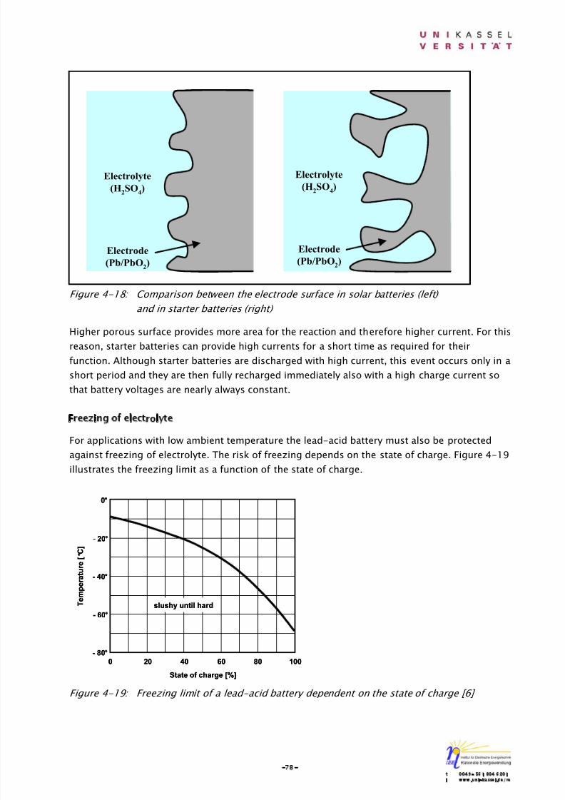
8/14/2019 Photovoltaic Systems Technology SS 2003
http://slidepdf.com/reader/full/photovoltaic-systems-technology-ss-2003 82/155
-78-t 0049- 561 804 6201i www.uni-kassel.de/re
Figure 4-18: Comparison between the electrode surface in solar batteries (left)
and in starter batteries (right)
Higher porous surface provides more area for the reaction and therefore higher current. For this
reason, starter batteries can provide high currents for a short time as required for their
function. Although starter batteries are discharged with high current, this event occurs only in a
short period and they are then fully recharged immediately also with a high charge current so
that battery voltages are nearly always constant.
Freezing of electrolyte
For applications with low ambient temperature the lead-acid battery must also be protected
against freezing of electrolyte. The risk of freezing depends on the state of charge. Figure 4-19
illustrates the freezing limit as a function of the state of charge.
Figure 4-19: Freezing limit of a lead-acid battery dependent on the state of charge [6]
- 80°
- 60°
- 40°
- 20°
0°
0 20 40 60 80 100
State of charge [%]
T e m p e r a t u r e [ C ]
slushy until hard
- 80°
- 60°
- 40°
- 20°
0°
0 20 40 60 80 100
State of charge [%]
T e m p e r a t u r e [ C ]
slushy until hard
Electrode
(Pb/PbO2)
Electrolyte
(H2SO
4)
Electrode
(Pb/PbO2)
Electrolyte
(H2SO
4)
Electrode
(Pb/PbO2)
Electrolyte
(H2SO
4)
Electrode
(Pb/PbO2)
Electrolyte
(H2SO
4)

8/14/2019 Photovoltaic Systems Technology SS 2003
http://slidepdf.com/reader/full/photovoltaic-systems-technology-ss-2003 83/155
-79-t 0049- 561 804 6201i www.uni-kassel.de/re
Cycle life of lead-acid batteries
The cycle life refers to a capability of the battery to withstand a certain number of
charge/discharge cycles of given depth of discharge (DOD). Since the lifetime of the battery
also depends on the average depth of discharge during cycling (expressed in % of rated
capacity), the cycling capability may be more conveniently expressed by multiplying thisaverage depth of discharge by the battery lifetime expressed in number of cycles. The result is
called the nominal cycling capability , which is expressed as the number of equivalent 100 %
nominal capacity cycles.
The starter battery typically has a low cycling capability of less than 100 nominal cycles, which
means that it is able to withstand for example 500 cycles of maximally 20 % depth of discharge.
The battery appropriate for PV application requires a good cycling capability of at least 500
nominal cycles, which means that it should be able to withstand for example 1000 cycles of 50
% depth of discharge (Fig. 4-20) [1].
Figure 4-20: Cycle life as a function of deep of discharge (Source: VARTA special report 3/1987)
4.3.4 The battery capacity
Previously, the storage capacity of a battery is expressed in Ah (Ampere-hours) showing how
many hours a certain current can be taken from the charged battery until the battery is
discharged, i.e. until the battery voltage drops to the discharge voltage threshold.
Nowadays, it might be more favourable to express a battery capacity in dischargeable energy,
namely Wh (Watt-hours) or kWh (kilowatt-hours). However, these two ways of expressing the
battery capacity are equivalent because they are related via the battery voltage, i.e. Ah ⋅ V = Wh.
Unfortunately, the capacity of a battery is not a constant quantity, but depends on the amount
of discharge current. The manufacturers give therefore the rated capacity of their batteries
always with regard to a certain discharge current.
0
20
40
60
80
0 1000 2000 3000 4000 5000
Cycle life [cycles]
D e p t h o f d i s c h a r g e [ % ]
100
100
Industrial batteries
Consumer
(starter)batteries
0
20
40
60
80
0 1000 2000 3000 4000 5000
Cycle life [cycles]
D e p t h o f d i s c h a r g e [ % ]
100
100
Industrial batteries
Consumer
(starter)batteries

8/14/2019 Photovoltaic Systems Technology SS 2003
http://slidepdf.com/reader/full/photovoltaic-systems-technology-ss-2003 84/155
8/14/2019 Photovoltaic Systems Technology SS 2003
http://slidepdf.com/reader/full/photovoltaic-systems-technology-ss-2003 85/155
-81-t 0049- 561 804 6201i www.uni-kassel.de/re
charging (Q C). Self-discharge will affect coulombic efficiency. Furthermore, it is reduced
particularly by the secondary reaction during charging, i.e. gassing.
ηI = Q D / Q C (4-19)
The battery will usually need more charge than was taken out to fill it back up to its startingpoint. Typical average coulombic efficiencies are 80 – 85 % for stand-alone PV systems, with
winter efficiencies increasing to 90 – 95 %, due to higher coulombic efficiencies when the
battery is at a lower state of charge and most of the charge going straight to the load, rather
than into the batteries.
The voltage efficiency, which is determined by the average discharge voltage (VD) and average
charging voltage (VC), is lowered particularly by internal resistance of the battery. It is also
measured at a constant discharge rate and reflecting the fact that charge is recalled from the
battery at a lower voltage than was necessary to put the charge into the battery.
ηV = VD / VC (4-20)
ηΣ should be as high as possible, to be able to pass the biggest proportion of the energy in the
battery, which is generated by the PV generator, further to consumers [4, 5].
Self-discharge
The battery discharges itself even without load connected. This effect is caused by secondary
reactions at it electrodes and proceeds faster with higher temperature or older battery [7].
Thermodynamic instability of the active materials and electrolytes as well as internal- and
external short-circuits lead to capacity losses, which are defined as self-discharge. This loss
should be small, particularly according to annual storage.
Maintenance cost
The maintenance, e.g. water refilling in case of lead-acid batteries, should be kept as low as
possible.
Easy installation and operation
Since batteries are driven often also from non-experts. Easy installation and operation aretherefore favourable.
Power
In special cases battery must be highly loadable for a short time, e.g. at the start of diesel
generators or in case of momentary power extension of PV systems [4, 5].
There are many types of batteries potentially available for use in stand-alone PV systems.
Useful data of available batteries given in Table 4-1 are approximated values and are provided
as a guideline. More information can be found in [1, 2, 4, 5, 7].
Type Cycle life until
80 % DOD
Investment
cost [€/kWh]
Specific kWh
cost [€/kWhΣ]
ηI [%] Self-discharge
[%/month]
Temp. range
[°C]

8/14/2019 Photovoltaic Systems Technology SS 2003
http://slidepdf.com/reader/full/photovoltaic-systems-technology-ss-2003 86/155
-82-t 0049- 561 804 6201i www.uni-kassel.de/re
Pb 500...1500 85...350 0.17…0.30 > 80 3…4 -15°...+50°
NiCd 1500...3500 650…1500 0.30…1.00 71 6…20 -40°...+45°
NiFe 3000 1000 0.33 55 40 0°…+40°
Table 4-1: Comparison between selection criteria of available batteries [4]
Since many values are dependent on charge- and discharge conditions, they have not been
standardized for PV applications and for test purposes until now. Therefore, the comparison
between batteries and selection of the most suitable one for each application are not easy. Due
to particular operating conditions with PV applications in practical operation, the cycle life given
by manufacturer (and in Table 4-1) for cycling load can be reduced more than half.
According to Table 4-1 it follows that in most cases the lead-acid batteries would be the best
choices for PV applications. The selection of suitable choices is to orient in application purpose
[4].
Lead-acid batteries come in a variety of types: deep or shallow cycling, gelled batteries,batteries with captive or liquid electrolyte, sealed or open batteries.
Sealed batteries are regulated to allow for evolution of excess hydrogen gas. However, catalytic
converters are used to convert as much evolved hydrogen and oxygen back to water as
possible. They are called “sealed” because electrolyte cannot be added. They require stringent
charging controls but less maintenance than open batteries.
Open- or flooded electrolyte batteries contain an excess of electrolyte and gassing is used to
reduce electrolyte stratification. The charging regime need not be stringent. However,
electrolyte must be replenished frequently and the battery housing must be well ventilated to
prevent the build-up of hydrogen gas.
Lead-acid batteries are produced with variety of plate types:
o) Pure lead plates have to be handled extremely carefully since the lead is soft and easily
damaged. However, they provide low self-discharge rates and long expectancy.
p) Calcium can be added to the plates (giving lead-calcium plates) to provide strength.
Their initial cost is less than that of pure lead-acid batteries, but they are not suitable
for repeated deep discharge and have slightly shorter lifetimes.
q) Antimony is also often added to lead plates for strength. Lead-antimony batteries are
common in automotive applications. They are substantially cheaper than pure lead or
lead-calcium batteries but have shorter lives and much higher self-discharge rates. In
addition, they degrade rapidly when deep cycled and need to be kept almost fully
charged at all times. They are consequently not ideal for use in stand-alone PV
applications. Lead-antimony batteries are usually only available as “open” batteries, due
to the high rate of electrolyte usage and consequent need for topping-up regularly [5]
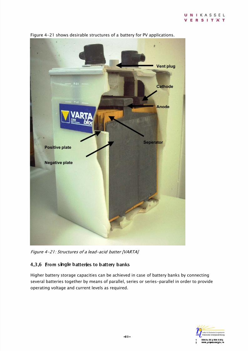
8/14/2019 Photovoltaic Systems Technology SS 2003
http://slidepdf.com/reader/full/photovoltaic-systems-technology-ss-2003 87/155
-83-t 0049- 561 804 6201i www.uni-kassel.de/re
Figure 4-21 shows desirable structures of a battery for PV applications.
Figure 4-21: Structures of a lead-acid batter [VARTA]
4.3.6 From single batteries to battery banks
Higher battery storage capacities can be achieved in case of battery banks by connecting
several batteries together by means of parallel, series or series-parallel in order to provide
operating voltage and current levels as required.
Anode
Cathode
Negative plate
Positive plate
Vent plug
Seperator
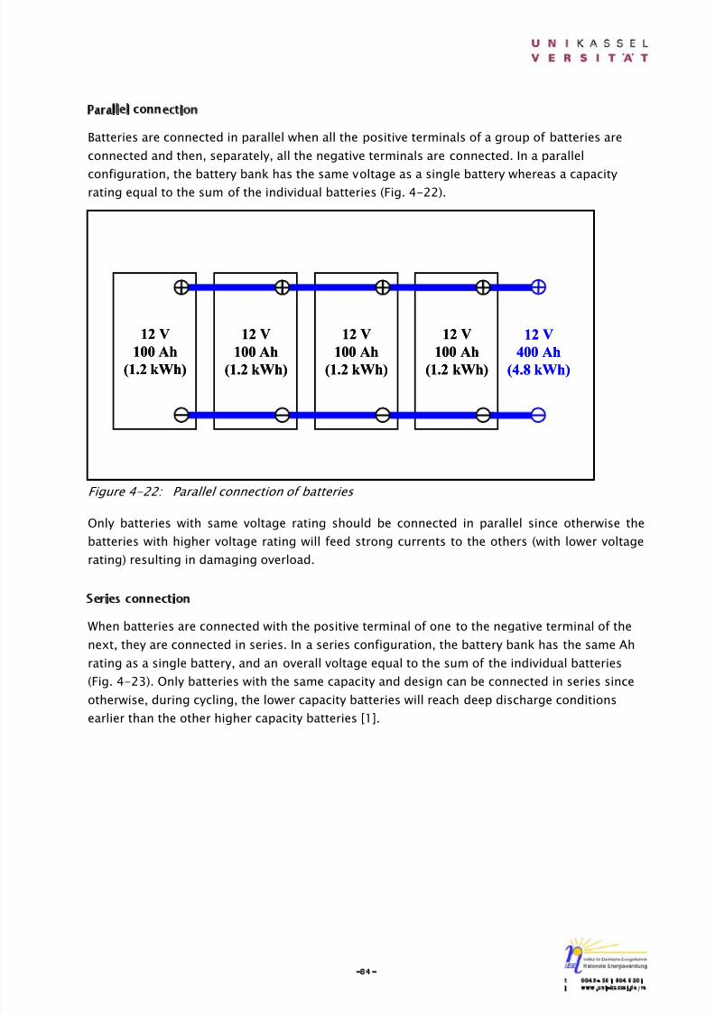
8/14/2019 Photovoltaic Systems Technology SS 2003
http://slidepdf.com/reader/full/photovoltaic-systems-technology-ss-2003 88/155
-84-t 0049- 561 804 6201i www.uni-kassel.de/re
Parallel connection
Batteries are connected in parallel when all the positive terminals of a group of batteries are
connected and then, separately, all the negative terminals are connected. In a parallel
configuration, the battery bank has the same voltage as a single battery whereas a capacityrating equal to the sum of the individual batteries (Fig. 4-22).
Figure 4-22: Parallel connection of batteries
Only batteries with same voltage rating should be connected in parallel since otherwise the
batteries with higher voltage rating will feed strong currents to the others (with lower voltage
rating) resulting in damaging overload.
Series connection
When batteries are connected with the positive terminal of one to the negative terminal of the
next, they are connected in series. In a series configuration, the battery bank has the same Ah
rating as a single battery, and an overall voltage equal to the sum of the individual batteries
(Fig. 4-23). Only batteries with the same capacity and design can be connected in series since
otherwise, during cycling, the lower capacity batteries will reach deep discharge conditions
earlier than the other higher capacity batteries [1].
12 V
100 Ah(1.2 kWh)
12 V
100 Ah(1.2 kWh)
12 V
100 Ah(1.2 kWh)
12 V
100 Ah(1.2 kWh)
12 V
400 Ah(4.8 kWh)
12 V
100 Ah(1.2 kWh)
12 V
100 Ah(1.2 kWh)
12 V
100 Ah(1.2 kWh)
12 V
100 Ah(1.2 kWh)
12 V
400 Ah(4.8 kWh)
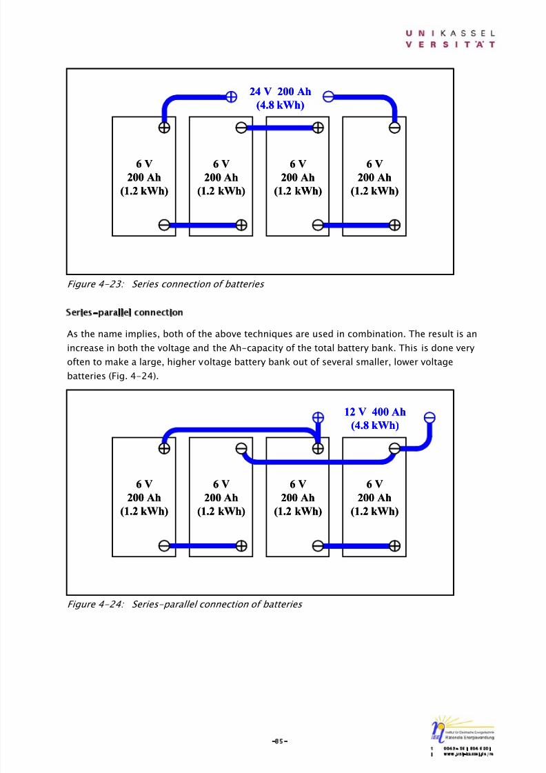
8/14/2019 Photovoltaic Systems Technology SS 2003
http://slidepdf.com/reader/full/photovoltaic-systems-technology-ss-2003 89/155
-85-t 0049- 561 804 6201i www.uni-kassel.de/re
Figure 4-23: Series connection of batteries
Series-parallel connection
As the name implies, both of the above techniques are used in combination. The result is an
increase in both the voltage and the Ah-capacity of the total battery bank. This is done very
often to make a large, higher voltage battery bank out of several smaller, lower voltage
batteries (Fig. 4-24).
Figure 4-24: Series-parallel connection of batteries
6 V
200 Ah
(1.2 kWh)
6 V
200 Ah
(1.2 kWh)
6 V
200 Ah
(1.2 kWh)
6 V
200 Ah
(1.2 kWh)
24 V 200 Ah
(4.8 kWh)
6 V
200 Ah
(1.2 kWh)
6 V
200 Ah
(1.2 kWh)
6 V
200 Ah
(1.2 kWh)
6 V
200 Ah
(1.2 kWh)
24 V 200 Ah
(4.8 kWh)
6 V
200 Ah
(1.2 kWh)
6 V
200 Ah
(1.2 kWh)
6 V
200 Ah
(1.2 kWh)
6 V
200 Ah
(1.2 kWh)
12 V 400 Ah
(4.8 kWh)
6 V
200 Ah
(1.2 kWh)
6 V
200 Ah
(1.2 kWh)
6 V
200 Ah
(1.2 kWh)
6 V
200 Ah
(1.2 kWh)
12 V 400 Ah
(4.8 kWh)
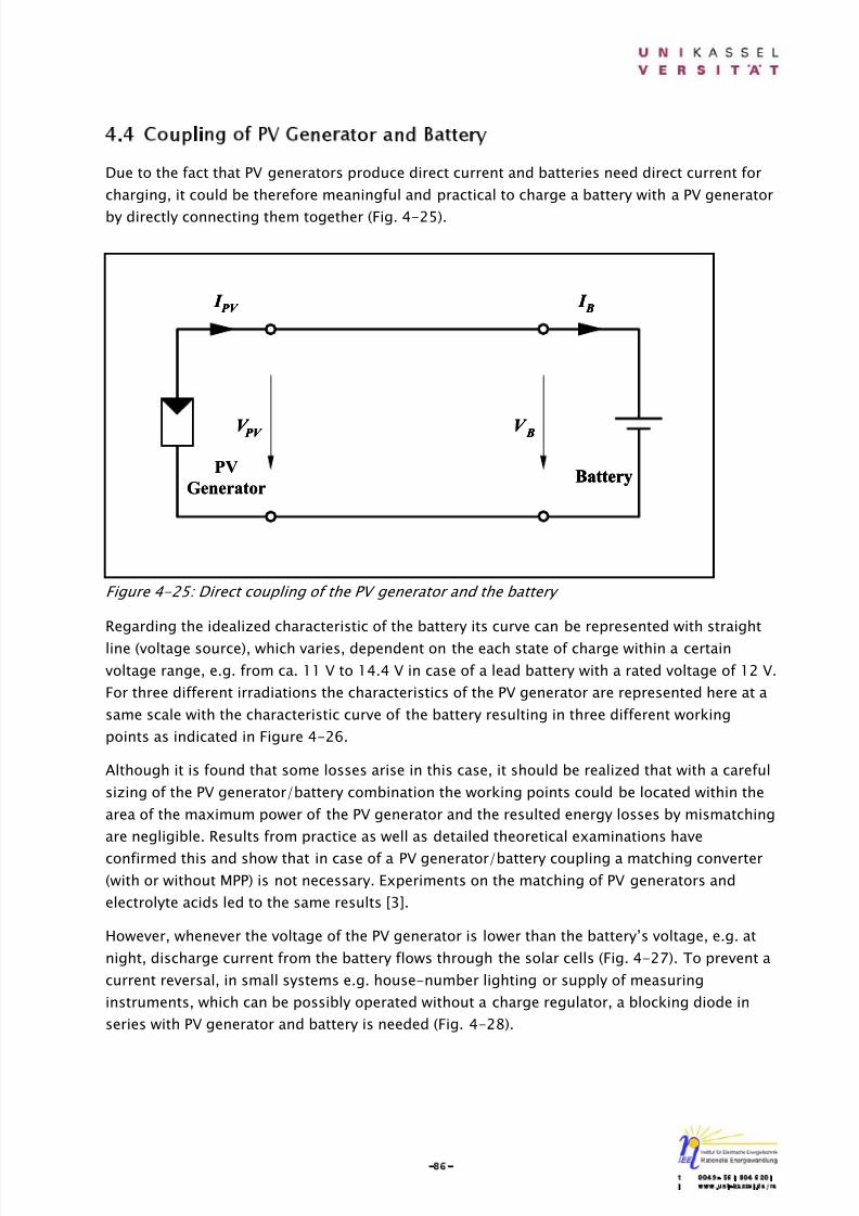
8/14/2019 Photovoltaic Systems Technology SS 2003
http://slidepdf.com/reader/full/photovoltaic-systems-technology-ss-2003 90/155
-86-t 0049- 561 804 6201i www.uni-kassel.de/re
4.4 Coupling of PV Generator and Battery
Due to the fact that PV generators produce direct current and batteries need direct current for
charging, it could be therefore meaningful and practical to charge a battery with a PV generator
by directly connecting them together (Fig. 4-25).
Figure 4-25: Direct coupling of the PV generator and the battery
Regarding the idealized characteristic of the battery its curve can be represented with straight
line (voltage source), which varies, dependent on the each state of charge within a certain
voltage range, e.g. from ca. 11 V to 14.4 V in case of a lead battery with a rated voltage of 12 V.
For three different irradiations the characteristics of the PV generator are represented here at a
same scale with the characteristic curve of the battery resulting in three different working
points as indicated in Figure 4-26.
Although it is found that some losses arise in this case, it should be realized that with a careful
sizing of the PV generator/battery combination the working points could be located within the
area of the maximum power of the PV generator and the resulted energy losses by mismatching
are negligible. Results from practice as well as detailed theoretical examinations have
confirmed this and show that in case of a PV generator/battery coupling a matching converter
(with or without MPP) is not necessary. Experiments on the matching of PV generators and
electrolyte acids led to the same results [3].
However, whenever the voltage of the PV generator is lower than the battery’s voltage, e.g. at
night, discharge current from the battery flows through the solar cells (Fig. 4-27). To prevent a
current reversal, in small systems e.g. house-number lighting or supply of measuring
instruments, which can be possibly operated without a charge regulator, a blocking diode in
series with PV generator and battery is needed (Fig. 4-28).
I B
Battery
V B
I PV
V PV
PV
Generator
I B
I B
BatteryBattery
V BV B
I PV
I PV
V PV V PV
PV
Generator
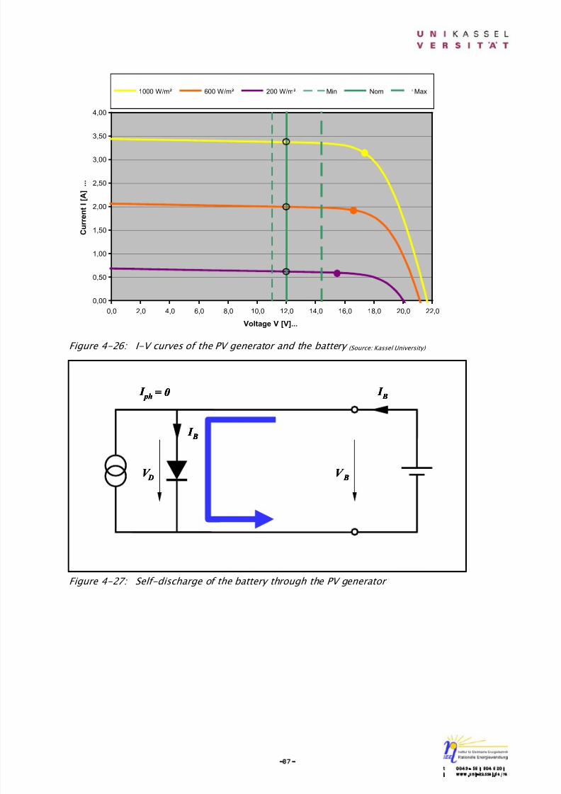
8/14/2019 Photovoltaic Systems Technology SS 2003
http://slidepdf.com/reader/full/photovoltaic-systems-technology-ss-2003 91/155
-87-t 0049- 561 804 6201i www.uni-kassel.de/re
Figure 4-26: I-V curves of the PV generator and the battery (Source: Kassel University)
Figure 4-27: Self-discharge of the battery through the PV generator
V D
I B
I ph = 0
I B
V B
V D
V D
I B
I B
I ph = 0 I ph = 0
I B
I B
V B
V B
0,00
0,50
1,00
1,50
2,00
2,50
3,00
3,50
4,00
0,0 2,0 4,0 6,0 8,0 10,0 12,0 14,0 16,0 18,0 20,0 22,0
Voltage V [V]...
C u r r e n t I [ A ] . . .
1000 W/m² 600 W/m² 200 W/m² Min Nom Max
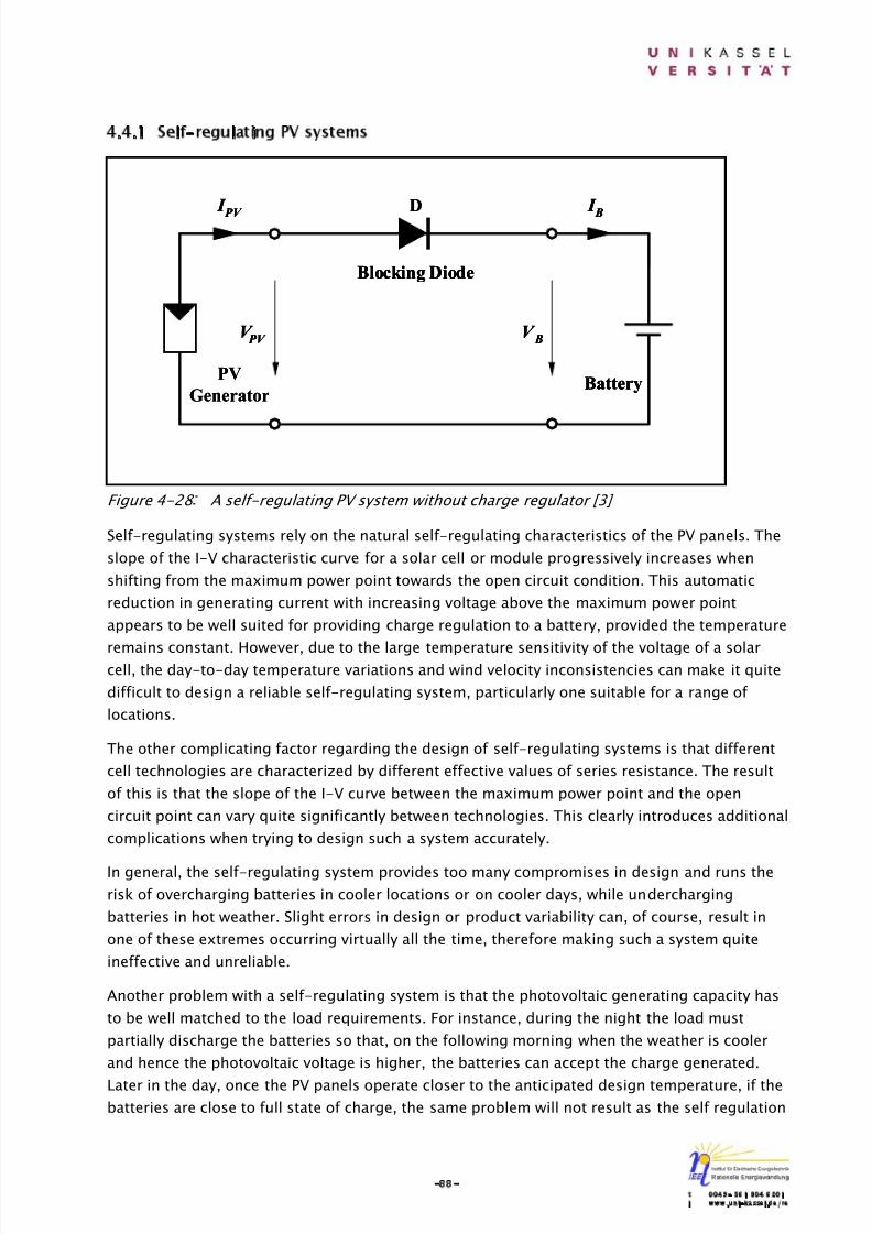
8/14/2019 Photovoltaic Systems Technology SS 2003
http://slidepdf.com/reader/full/photovoltaic-systems-technology-ss-2003 92/155
-88-t 0049- 561 804 6201i www.uni-kassel.de/re
4.4.1 Self-regulating PV systems
Figure 4-28 : A self-regulating PV system without charge regulator [3]
Self-regulating systems rely on the natural self-regulating characteristics of the PV panels. The
slope of the I-V characteristic curve for a solar cell or module progressively increases when
shifting from the maximum power point towards the open circuit condition. This automatic
reduction in generating current with increasing voltage above the maximum power point
appears to be well suited for providing charge regulation to a battery, provided the temperature
remains constant. However, due to the large temperature sensitivity of the voltage of a solarcell, the day-to-day temperature variations and wind velocity inconsistencies can make it quite
difficult to design a reliable self-regulating system, particularly one suitable for a range of
locations.
The other complicating factor regarding the design of self-regulating systems is that different
cell technologies are characterized by different effective values of series resistance. The result
of this is that the slope of the I-V curve between the maximum power point and the open
circuit point can vary quite significantly between technologies. This clearly introduces additional
complications when trying to design such a system accurately.
In general, the self-regulating system provides too many compromises in design and runs the
risk of overcharging batteries in cooler locations or on cooler days, while undercharging
batteries in hot weather. Slight errors in design or product variability can, of course, result in
one of these extremes occurring virtually all the time, therefore making such a system quite
ineffective and unreliable.
Another problem with a self-regulating system is that the photovoltaic generating capacity has
to be well matched to the load requirements. For instance, during the night the load must
partially discharge the batteries so that, on the following morning when the weather is cooler
and hence the photovoltaic voltage is higher, the batteries can accept the charge generated.
Later in the day, once the PV panels operate closer to the anticipated design temperature, if thebatteries are close to full state of charge, the same problem will not result as the self regulation
I PV
V PV
PV
Generator
Blocking Diode
D I B
Battery
V B
I PV
I PV
V PV V PV
PV
Generator
Blocking DiodeBlocking Diode
D I B
I B
BatteryBattery
V BV B
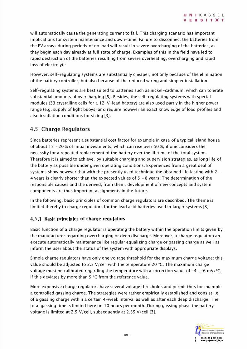
8/14/2019 Photovoltaic Systems Technology SS 2003
http://slidepdf.com/reader/full/photovoltaic-systems-technology-ss-2003 93/155
-89-t 0049- 561 804 6201i www.uni-kassel.de/re
will automatically cause the generating current to fall. This charging scenario has important
implications for system maintenance and down-time. Failure to disconnect the batteries from
the PV arrays during periods of no load will result in severe overcharging of the batteries, as
they begin each day already at full state of charge. Examples of this in the field have led to
rapid destruction of the batteries resulting from severe overheating, overcharging and rapid
loss of electrolyte.
However, self-regulating systems are substantially cheaper, not only because of the elimination
of the battery controller, but also because of the reduced wiring and simpler installation.
Self-regulating systems are best suited to batteries such as nickel-cadmium, which can tolerate
substantial amounts of overcharging [5]. Besides, the self-regulating systems with special
modules (33 crystalline cells for a 12-V-lead battery) are also used partly in the higher power
range (e.g. supply of light buoys) and require however an exact knowledge of load profiles and
also irradiation conditions for sizing [3].
4.5 Charge Regulators
Since batteries represent a substantial cost factor for example in case of a typical island house
of about 15 – 20 % of initial investments, which can rise over 50 %, if one considers the
necessity for a repeated replacement of the battery over the lifetime of the total system.
Therefore it is aimed to achieve, by suitable charging and supervision strategies, as long life of
the battery as possible under given operating conditions. Experiences from a great deal of
systems show however that with the presently used technique the obtained life lasting with 2 –
4 years is clearly shorter than the expected values of 5 – 8 years. The determination of the
responsible causes and the derived, from them, development of new concepts and systemcomponents are thus important assignments in the future.
In the following, basic principles of common charge regulators are described. The theme is
limited thereby to charge regulators for the lead acid batteries used in larger systems [3].
4.5.1 Basic principles of charge regulators
Basic function of a charge regulator is operating the battery within the operation limits given by
the manufacturer regarding overcharging or deep discharge. Moreover, a charge regulator can
execute automatically maintenance like regular equalizing charge or gassing charge as well as
inform the user about the status of the system with appropriate displays.
Simple charge regulators have only one voltage threshold for the maximum charge voltage: this
value should be adjusted to 2.3 V/cell with the temperature 20 °C. The maximum charge
voltage must be calibrated regarding the temperature with a correction value of -4…-6 mV/°C,
if this deviates by more than 5 °C from the reference value.
More expensive charge regulators have several voltage thresholds and permit thus for example
a controlled gassing charge. The strategies were rather empirically established and consist i.e.
of a gassing charge within a certain 4-week interval as well as after each deep discharge. The
total gassing time is limited here on 10 hours per month. During gassing phase the batteryvoltage is limited at 2.5 V/cell, subsequently at 2.35 V/cell [3].
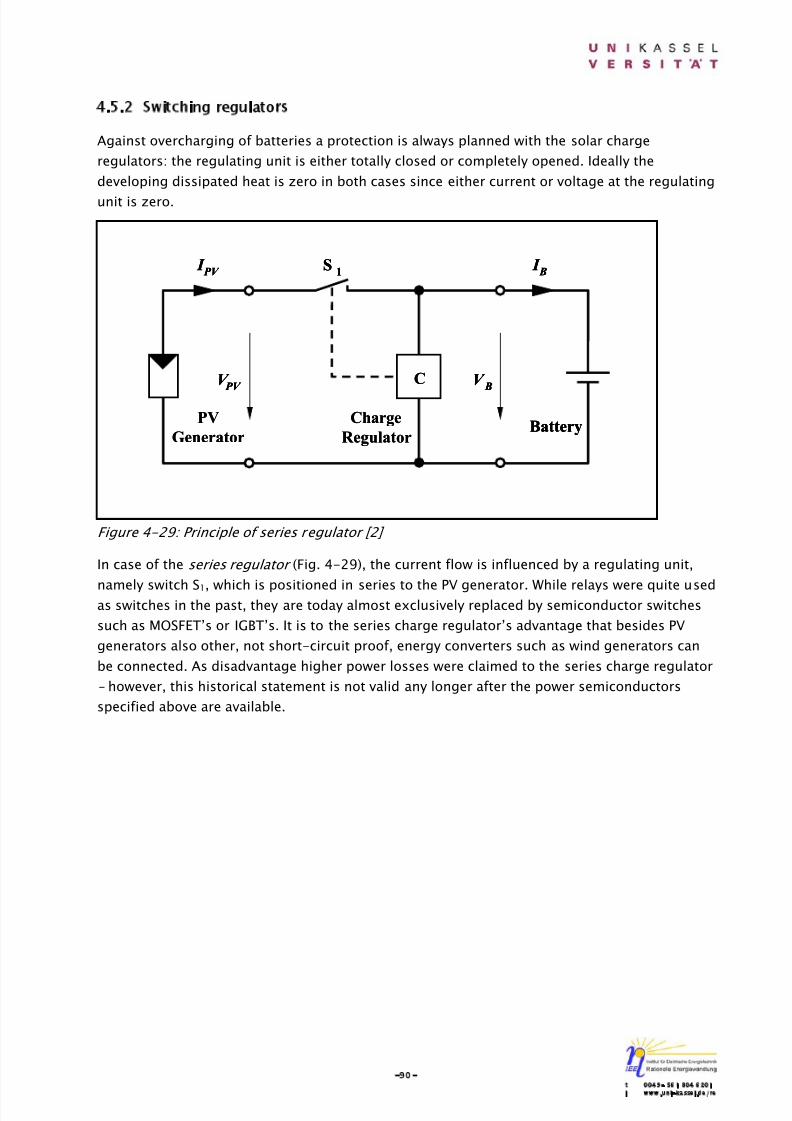
8/14/2019 Photovoltaic Systems Technology SS 2003
http://slidepdf.com/reader/full/photovoltaic-systems-technology-ss-2003 94/155
-90-t 0049- 561 804 6201i www.uni-kassel.de/re
4.5.2 Switching regulators
Against overcharging of batteries a protection is always planned with the solar charge
regulators: the regulating unit is either totally closed or completely opened. Ideally the
developing dissipated heat is zero in both cases since either current or voltage at the regulating
unit is zero.
Figure 4-29: Principle of series regulator [2]
In case of the series regulator (Fig. 4-29), the current flow is influenced by a regulating unit,
namely switch S1, which is positioned in series to the PV generator. While relays were quite usedas switches in the past, they are today almost exclusively replaced by semiconductor switches
such as MOSFET’s or IGBT’s. It is to the series charge regulator’s advantage that besides PV
generators also other, not short-circuit proof, energy converters such as wind generators can
be connected. As disadvantage higher power losses were claimed to the series charge regulator
– however, this historical statement is not valid any longer after the power semiconductors
specified above are available.
S1
C
Charge
Regulator
I PV
V PV
PV
Generator
I B
Battery
V B
S1
S1
C
Charge
Regulator
I PV
I PV
V PV
V PV
PV
Generator
I B
I B
BatteryBattery
V B
V B

8/14/2019 Photovoltaic Systems Technology SS 2003
http://slidepdf.com/reader/full/photovoltaic-systems-technology-ss-2003 95/155
-91-t 0049- 561 804 6201i www.uni-kassel.de/re
Figure 4-30: Principle of shunt regulator [2]
Regarding the parallel- or shunt regulator (Fig. 4-30) the characteristic of PV generators is
applied, namely being able to be short-circuited arbitrarily for a long time. During charging the
PV generator current flows through the diode D into the battery. As achieving the maximum
charge voltage the PV generator is short-circuited by the regulating unit according to one of the
further strategies described below, so that no more charging current can flow. The diode
prevents here, on one hand, the current reversal from the battery into this short-circuited path;
on the other hand it prevents discharging of the battery to the unlighted PV generator at night.
It is favourable with the shunt regulator since it makes a charging current also in the case of a
completely discharged battery flow through the diode and thus the system starts reliably. This
is however not guaranteed in the case of the series regulator with a bad connection design
since there is no energy available to turn on the switch.
Moreover, as mentioned before, if the battery is connected to the load, the deep discharge
protection (DDP) is required, which is represented by the switch S2 in Figure 4-31.
The hybrid regulator represents a modification of the shunt regulator, with which in the
charging phase the blocking diode is bridged by a switch situated in parallel and the dissipated
heat is again minimized. However, it must be emphasized here that this is not relevant to theenergy gains for the energy balance of the total system but, in the foreground of discussion,
rather the reduction of the developing dissipated heat in the regulator that leads to savings at
heat sinks and housings, in addition, contributes to a increased reliability.
S1
Charge
Regulator
C
I Shunt
D I B
Battery
V B
I PV
V PV
PV
Generator
S1
S1
Charge
Regulator
C
I Shunt I Shunt
D I B
I B
BatteryBattery
V B
V B
I PV
I PV
V PV
V PV
PV
Generator

8/14/2019 Photovoltaic Systems Technology SS 2003
http://slidepdf.com/reader/full/photovoltaic-systems-technology-ss-2003 96/155
-92-t 0049- 561 804 6201i www.uni-kassel.de/re
Figure 4-31: Shunt regulator with deep discharge protection (DDP) [2]
In case of higher power of PV generator, the so-called sub array switching is applied, with
which the generator is divided into several subfields that operate at a time over assigned
sections on a combined battery. Here either all sections can be controlled together by an
individual control section or can be however advantageously switched off after a given load
strategy, what provides a better control of the total charging current.
An applied method, only sorted in systems of higher voltage, is the so-called partial shunting ,
with which only one part of the modules interconnected in series is short-circuited by an
additional connection and thus the generator voltage for a further charging becomes too low
[3].
At the first achieving of the maximum charge voltage a battery is not yet completely charged. It
is just fully charged if the whole lead sulphate is converted into lead and lead oxide [7]. To
reach the full charging the battery must be further charged for a longer period with constant
voltage, whereby the charging current decreases slowly (I-V charging). This behavior can be
achieved by suitable control of the regulating unit with the series- and also shunt regulator,
whereby two realistic possibilities are available:
By means of two-step regulator the current, as reaching the maximum charge voltage, isinterrupted (by opening the regulating unit of the series regulator or closing in the case of
shunt regulator), thus the battery voltage drops (Fig. 4-32) [3]. At this moment a characteristic
of the battery has an effect: the battery behaves like a big capacitor. Therefore, the battery
voltage does not drop immediately, but rather follows the discharge curve of a capacitor [6].
S1
Charge
Regulator
C
I Shunt
D S2
Rload Battery
I PV
V PV
PV
Generator
S1
S1
Charge
Regulator
C
I Shunt I Shunt
D S2
S2
Rload
Rload Battery
I PV
I PV
V PV
V PV
PV
Generator

8/14/2019 Photovoltaic Systems Technology SS 2003
http://slidepdf.com/reader/full/photovoltaic-systems-technology-ss-2003 97/155
-93-t 0049- 561 804 6201i www.uni-kassel.de/re
Figure 4-32: Voltage and current characteristics during charging [2]
As reaching a lower voltage threshold, about some millivolts [3], the charging current is again
connected and the voltage rises then corresponding to the charging curve of a capacitor. With
increase in state of charge of the battery the resulting charging phases become ever shorter
and intervening pauses become longer, so that the average value of charging current decreases
as required [6]. The cycle duration of the described phenomenon is not constant, but depends
on the state of charge, battery capacity, the charging- or discharge current as well as selectedvoltage hysteresis: it can therefore vary within the range of milliseconds up to minutes.
The pulse-width-modulated (PWM-) charge regulator operates in principle similarly, however,
the switching frequency of the switch is fixed given here by a timer with e.g. 100 Hz. Firstly the
full charging current flows here also, whereby during approximation to the maximum charge
voltage the relation of charging time to the total cycle time is modified continuously by an
appropriate PWM-modulator of 1 until 0. As indicated in the figure above, this has thereby the
required reduction of the average charging current as a result [3].
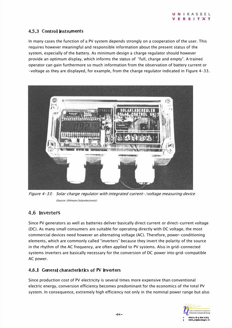
8/14/2019 Photovoltaic Systems Technology SS 2003
http://slidepdf.com/reader/full/photovoltaic-systems-technology-ss-2003 98/155
-94-t 0049- 561 804 6201i www.uni-kassel.de/re
4.5.3 Control instruments
In many cases the function of a PV system depends strongly on a cooperation of the user. This
requires however meaningful and responsible information about the present status of the
system, especially of the battery. As minimum design a charge regulator should however
provide an optimum display, which informs the status of “full, charge and empty”. A trained
operator can gain furthermore so much information from the observation of battery current or
-voltage as they are displayed, for example, from the charge regulator indicated in Figure 4-33.
Figure 4-33: Solar charge regulator with integrated current-/voltage measuring device
(Source: Uhlmann Solarelectronic)
4.6 Inverters
Since PV generators as well as batteries deliver basically direct current or direct-current voltage
(DC). As many small consumers are suitable for operating directly with DC voltage, the mostcommercial devices need however an alternating voltage (AC). Therefore, power-conditioning
elements, which are commonly called “inverters” because they invert the polarity of the source
in the rhythm of the AC frequency, are often applied to PV systems. Also in grid-connected
systems inverters are basically necessary for the conversion of DC power into grid-compatible
AC power.
4.6.1 General characteristics of PV inverters
Since production cost of PV electricity is several times more expensive than conventional
electric energy, conversion efficiency becomes predominant for the economics of the total PVsystem. In consequence, extremely high efficiency not only in the nominal power range but also
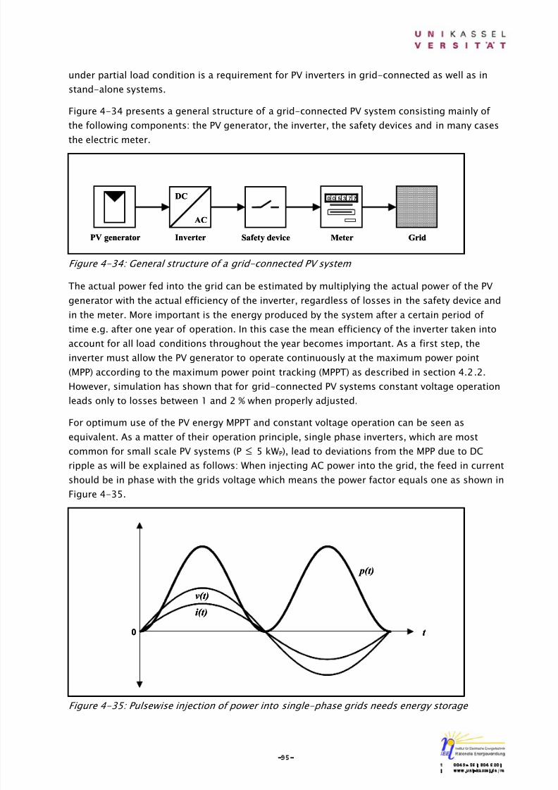
8/14/2019 Photovoltaic Systems Technology SS 2003
http://slidepdf.com/reader/full/photovoltaic-systems-technology-ss-2003 99/155
-95-t 0049- 561 804 6201i www.uni-kassel.de/re
under partial load condition is a requirement for PV inverters in grid-connected as well as in
stand-alone systems.
Figure 4-34 presents a general structure of a grid-connected PV system consisting mainly of
the following components: the PV generator, the inverter, the safety devices and in many cases
the electric meter.
Figure 4-34: General structure of a grid-connected PV system
The actual power fed into the grid can be estimated by multiplying the actual power of the PV
generator with the actual efficiency of the inverter, regardless of losses in the safety device and
in the meter. More important is the energy produced by the system after a certain period of
time e.g. after one year of operation. In this case the mean efficiency of the inverter taken into
account for all load conditions throughout the year becomes important. As a first step, the
inverter must allow the PV generator to operate continuously at the maximum power point
(MPP) according to the maximum power point tracking (MPPT) as described in section 4.2.2.
However, simulation has shown that for grid-connected PV systems constant voltage operation
leads only to losses between 1 and 2 % when properly adjusted.
For optimum use of the PV energy MPPT and constant voltage operation can be seen as
equivalent. As a matter of their operation principle, single phase inverters, which are most
common for small scale PV systems (P ≤ 5 kWP), lead to deviations from the MPP due to DC
ripple as will be explained as follows: When injecting AC power into the grid, the feed in current
should be in phase with the grids voltage which means the power factor equals one as shown in
Figure 4-35.
Figure 4-35: Pulsewise injection of power into single-phase grids needs energy storage
Safety device Meter GridInverterPV generator
DC
AC
773500
Safety device Meter GridInverterPV generator
DC
AC
773500
0
p(t)
v(t)
i(t)
t 0
p(t)
v(t)
i(t)
t
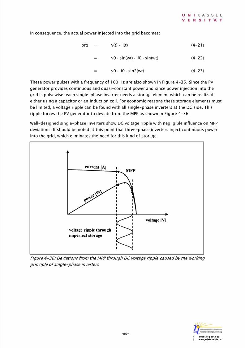
8/14/2019 Photovoltaic Systems Technology SS 2003
http://slidepdf.com/reader/full/photovoltaic-systems-technology-ss-2003 100/155
-96-t 0049- 561 804 6201i www.uni-kassel.de/re
In consequence, the actual power injected into the grid becomes:
p(t) = v(t) ⋅ i(t) (4-21)
= v0 ⋅ sin(wt) ⋅ i0 ⋅ sin(wt) (4-22)
= v0 ⋅ i0 ⋅ sin2(wt) (4-23)
These power pulses with a frequency of 100 Hz are also shown in Figure 4-35. Since the PV
generator provides continuous and quasi-constant power and since power injection into the
grid is pulsewise, each single-phase inverter needs a storage element which can be realized
either using a capacitor or an induction coil. For economic reasons these storage elements must
be limited, a voltage ripple can be found with all single-phase inverters at the DC side. This
ripple forces the PV generator to deviate from the MPP as shown in Figure 4-36.
Well-designed single-phase inverters show DC voltage ripple with negligible influence on MPPdeviations. It should be noted at this point that three-phase inverters inject continuous power
into the grid, which eliminates the need for this kind of storage.
Figure 4-36: Deviations from the MPP through DC voltage ripple caused by the working
principle of single-phase inverters
voltage [V]
current [A]
p o w e r [
W ]
MPP
voltage ripple through
imperfect storage
voltage [V]
current [A]
p o w e r [
W ]
MPP
voltage ripple through
imperfect storage

8/14/2019 Photovoltaic Systems Technology SS 2003
http://slidepdf.com/reader/full/photovoltaic-systems-technology-ss-2003 101/155
-97-t 0049- 561 804 6201i www.uni-kassel.de/re
4.6.2 Inverter principles
The symbol used to describe an inverter is shown in Figure 4-37.
Figure 4-37: Symbol used to describe an inverter
Square-wave inverters
A simple version of such an inverter is shown in Figure 4-38. AC at the primary windings of the
transformer is being produced by alternatively closing the S1 and S2. If S1 is closed, S2 is open
and vice versa. The resulting AC output voltage is of square-wave type, which may be used for
resistive-type loads such as incandescent light bulbs etc.
Figure 4-38: Layout of a simple inverter with square-wave AC output
Anyway, the two primary windings of the transformer can be reduced to one if two more
switches are used (Fig. 4-39).
AC outputDC input
∼AC outputDC input
∼
S1
S2
AC
output
DC
source
S1
S1
S2
S2
AC
output
DC
source
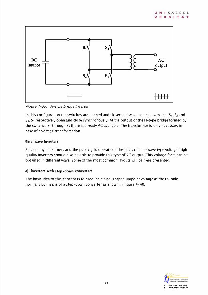
8/14/2019 Photovoltaic Systems Technology SS 2003
http://slidepdf.com/reader/full/photovoltaic-systems-technology-ss-2003 102/155
-98-t 0049- 561 804 6201i www.uni-kassel.de/re
Figure 4-39: H-type bridge inverter
In this configuration the switches are opened and closed pairwise in such a way that S1, S2 and
S3, S4 respectively open and close synchronously. At the output of the H-type bridge formed by
the switches S1 through S4 there is already AC available. The transformer is only necessary in
case of a voltage transformation.
Sine-wave inverters
Since many consumers and the public grid operate on the basis of sine-wave type voltage, high
quality inverters should also be able to provide this type of AC output. This voltage form can beobtained in different ways. Some of the most common layouts will be here presented.
a) Inverters with step-down converters
The basic idea of this concept is to produce a sine-shaped unipolar voltage at the DC side
normally by means of a step-down converter as shown in Figure 4-40.
AC
output
DC
source
S1
S3
S2S
4
AC
output
DC
source
S1
S1
S3
S3
S2S2S
4S
4

8/14/2019 Photovoltaic Systems Technology SS 2003
http://slidepdf.com/reader/full/photovoltaic-systems-technology-ss-2003 103/155
-99-t 0049- 561 804 6201i www.uni-kassel.de/re
Figure 4-40: The combination of a step-down converter with inverter according to
Fig. 4-38 or Fig. 4-39 allow producing sine-shaped AC output voltage
Since in this configuration the actual voltage and the corresponding current at the output of the
step-down converter is no longer constant, the resulting current at the input of the converter
will also fluctuate. In case of using PV generator used as a DC source, a storage capacitor C1
becomes necessary.
The quality of the voltage shape is normally described as total harmonic distortion (THD). The
THD is defined as sum of the amplitudes of all harmonic frequencies compared to the
amplitude of the fundamental signal (the 50 and 60 Hz frequency respectively). In this case
THD is determined by the switching frequency of S0 and by the inductance of L1. With modern
semiconductor switches this frequency can be realized in the range of 100 kHz, which keeps L1
small enough.
The voltage transformation between the DC source V 2 at the output of the step-down converter
can be given as:
V2 = V1 ⋅ T
t on (4-24)
Where t on is the on-time for switch so while T corresponds with the time of one switching
period. This principle, in which the desired output voltage is being produced by means of
variable on-time of the switch is called pulse-width modulation (PWM). The switches S1 and S2
in Figure 4-40 are needed to invert the polarity of every second half-wave in order to form the
AC output.
S0
D
S1
S2
C1
C1
L1
Battery
S0
S0
D
S1
S1
S2
S2
C1
C1
C1
C1
L1
L1
Battery
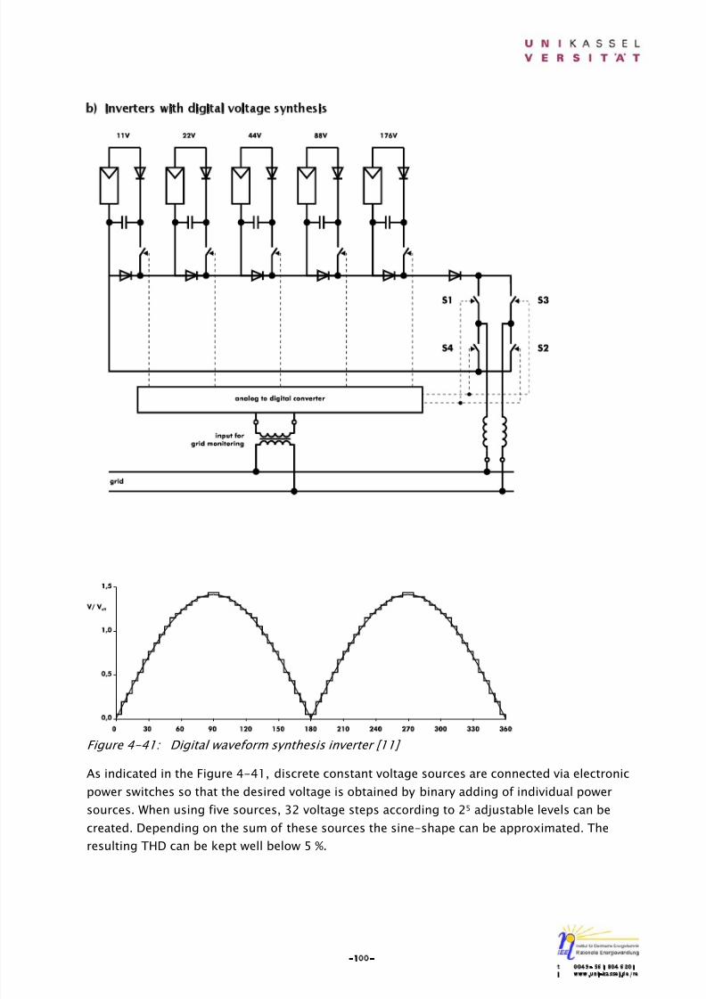
8/14/2019 Photovoltaic Systems Technology SS 2003
http://slidepdf.com/reader/full/photovoltaic-systems-technology-ss-2003 104/155
-100-t 0049- 561 804 6201i www.uni-kassel.de/re
b) Inverters with digital voltage synthesis
Figure 4-41: Digital waveform synthesis inverter [11]
As indicated in the Figure 4-41, discrete constant voltage sources are connected via electronic
power switches so that the desired voltage is obtained by binary adding of individual power
sources. When using five sources, 32 voltage steps according to 25 adjustable levels can be
created. Depending on the sum of these sources the sine-shape can be approximated. The
resulting THD can be kept well below 5 %.
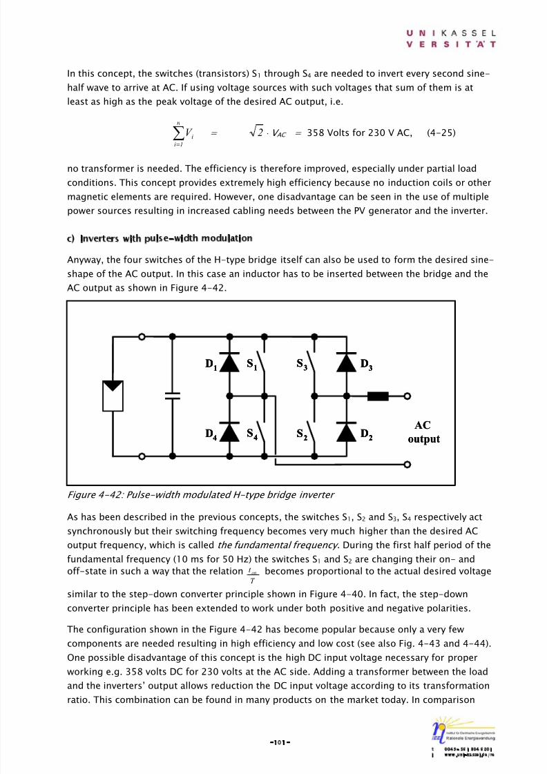
8/14/2019 Photovoltaic Systems Technology SS 2003
http://slidepdf.com/reader/full/photovoltaic-systems-technology-ss-2003 105/155
-101-t 0049- 561 804 6201i www.uni-kassel.de/re
In this concept, the switches (transistors) S1 through S4 are needed to invert every second sine-
half wave to arrive at AC. If using voltage sources with such voltages that sum of them is at
least as high as the peak voltage of the desired AC output, i.e.
∑=
n
1iiV = 2 ⋅ V AC = 358 Volts for 230 V AC, (4-25)
no transformer is needed. The efficiency is therefore improved, especially under partial load
conditions. This concept provides extremely high efficiency because no induction coils or other
magnetic elements are required. However, one disadvantage can be seen in the use of multiple
power sources resulting in increased cabling needs between the PV generator and the inverter.
c) Inverters with pulse-width modulation
Anyway, the four switches of the H-type bridge itself can also be used to form the desired sine-
shape of the AC output. In this case an inductor has to be inserted between the bridge and theAC output as shown in Figure 4-42.
Figure 4-42: Pulse-width modulated H-type bridge inverter
As has been described in the previous concepts, the switches S1, S2 and S3, S4 respectively act
synchronously but their switching frequency becomes very much higher than the desired AC
output frequency, which is called the fundamental frequency . During the first half period of thefundamental frequency (10 ms for 50 Hz) the switches S1 and S2 are changing their on- andoff-state in such a way that the relation
T
t on becomes proportional to the actual desired voltage
similar to the step-down converter principle shown in Figure 4-40. In fact, the step-down
converter principle has been extended to work under both positive and negative polarities.
The configuration shown in the Figure 4-42 has become popular because only a very few
components are needed resulting in high efficiency and low cost (see also Fig. 4-43 and 4-44).
One possible disadvantage of this concept is the high DC input voltage necessary for proper
working e.g. 358 volts DC for 230 volts at the AC side. Adding a transformer between the load
and the inverters’ output allows reduction the DC input voltage according to its transformation
ratio. This combination can be found in many products on the market today. In comparison
S1S
3
S2
AC
output
D1
D4
S4
D3
D2
S1S1S
3S
3
S2
S2
AC
output
D1
D1
D4
D4
S4S4
D3
D3
D2
D2

8/14/2019 Photovoltaic Systems Technology SS 2003
http://slidepdf.com/reader/full/photovoltaic-systems-technology-ss-2003 106/155
-102-t 0049- 561 804 6201i www.uni-kassel.de/re
with the transformerless version, separation of the potential between source and load becomes
feasible. Reduced efficiency and increased investment costs are the consequences however.
The concept explained in the Figure 4-42 allows further operating in a reversed power flow.
This situation may occur for inverters in stand-alone mode if the load is of reactive type or it
surplus power from the AC side is used to charge the battery. In both cases variable AC voltagemust be transformed to the DC voltage level, which is always higher than any value of the AC
voltage as shown in Figure 4-43. By combining S2 and D3 in Figure 4-42, a complete step-down
converter can be realized this way for the positive AC voltage. For the negative part the
combination of S1 and D4 are forming the step-up converter for reversed power flow.
Figure 4-43: Left: Step-down conversion in the forward power flow mode
Right: Step-up conversion in the reversed power flow mode
The concept described above allows reversed power flow only in cases, in which the DC voltage
level is always higher than the peak voltage of the AC side, i.e. VDC ≥ 358 Volts for 230 Volts
AC. There are two possibilities to lower the DC voltage level however, namely to install a
transformer at the AC side or to install a bi-directional DC/DC converter at the DC side. Since a
conventional step-down converter as described before is not able to act as a step-up converter
in the reversed power flow mode either two converters in anti-parallel-mode or a different
conversion concept would be necessary. One topology developed by S. Cuk in 1977, which is
able to fulfill these requirements, is given in Figure 4-44.
DC voltage level DC voltage level
V V
AC voltage AC voltage
t t
DC voltage level DC voltage level
V V
AC voltage AC voltage
t t

8/14/2019 Photovoltaic Systems Technology SS 2003
http://slidepdf.com/reader/full/photovoltaic-systems-technology-ss-2003 107/155
-103-t 0049- 561 804 6201i www.uni-kassel.de/re
Figure 4-44: Bi-directional Cuk-converter
This conversion principle is actually able to perform step-up as well as step-down conversion
in both directions. Switches S1 and S2 operate complementary. The relation between the input
voltage V 1 and the output voltage V 2 becomes:
V 2 =
( )
−−⋅+
⋅−
onoff
ononoff
on1
t t
t 1 t t
t V (4-26)
The configuration shown in Figure 4-42 is also very well suited to be expanded into a three-
phase version as shown in Figure 4-45.
Figure 4-45: Three-phase PWM inverter
This type of inverter is normally suitable for a power range above 5 kW. Connection efforts at
the AC side are somewhat higher because three terminals have to be dealt with. The most
S1
S2
C1R 1
L1
R 2
L2
C2
V 2
V 1
S1
S1
S2
S2
C1C1R 1
R 1
L1
L1
R 2
R 2
L2
L2
C2
C2
V 2
V 2
V 1
V 1
S1
S2
L3
S5
S6
L1
S3
S4
L2
S1S1
S2
S2
L3L3
S5
S5
S6
S6
L1
L1
S3S3
S4
S4
L2
L2

8/14/2019 Photovoltaic Systems Technology SS 2003
http://slidepdf.com/reader/full/photovoltaic-systems-technology-ss-2003 108/155
-104-t 0049- 561 804 6201i www.uni-kassel.de/re
striking advantage of a three-phase concept can be seen in the fact that power output and thus
power input are absolutely constant. As a result, no storage capacitor at the DC input side is
needed. This concept can also be combined with a three-phase transformer in a way as has
been described before.
If potential separation between DC input and AC output is requested and if the bulky 50 Hz-transformer should be avoided, high-frequency (HF) transformer concepts may be used. Three
topologies using HF concepts will be here described.
In a first concept, the configuration as explained in Figure 4-40 is applied to high frequency
(some 100 kHz) using a high-frequency transformer. The high-frequency square-wave AC
output is then rectified as shown in Figure 4-46. Providing the desired DC voltage necessary for
PWM inversion according to the H-type bridge explained in Figure 4-42.
Figure 4-46: HF transformer combined with PWM H-type bridge inverter
In comparison with the low frequency concepts, it becomes obvious that the savings using the
HF transformer are widely being compensated by extra components. This might be one of the
reasons why HF concepts have not widely been used in inverters offered to the market.
When operating the high frequency generator as described in Figure 4-47 in the PWM mode, in
which the desired low frequency is being used for modulation, a PWM series of unipolar half-
waves are resulting after the rectifier at the secondary windings of the HF-transformer.
By means of the combination of L1 and C2 a unipolar series of sinusoidal half-waves are
resulting, which are finally inverted by the H-type bridge as described in Figure 4-37. The 100-Hz pulsewise power injection requests an adequate storage element, which is realized by means
of the capacitor C2. It should be noted that this storage function is realized with C2 in the
topology presented previously in Figure 4-46.
S1
S2
C1 C2
L1
L2
S1
S2
C1 C2
L1
L2

8/14/2019 Photovoltaic Systems Technology SS 2003
http://slidepdf.com/reader/full/photovoltaic-systems-technology-ss-2003 109/155
-105-t 0049- 561 804 6201i www.uni-kassel.de/re
Figure 4-47: HF transformer combined with PWM high-frequency generator at the input side
and a low frequency H-type bridge at the output side
Finally a HF concept is presented, in which AC is directly being produced at the secondary sideof the HF-transformer. In this case the non-controlled rectifier shown in Figure 4-47 has been
replaced by active switches combining the functions of rectification and inversion. This
configuration is presented in Figure 4-48. It should be noted that in this case the switches in
the H-type bridge have to be operated in the rhythm of the high frequency in contrast to the
topology described in Figure 4-47. Since transistors switched with higher frequencies have
higher losses as well as higher investment costs, the benefit of saving the passive rectifier used
in the concept given in Figure 4-47 might be compensated by these facts to a certain extend.
Figure 4-48: Direct AC synthesis at the secondary winding of the HF transformer.
The PWM high-frequency signal is inverted in the low-frequency rhythm and smoothed by
means of L and C2. C1 is needed to store the input energy in the rhythm, which equals twice the
low frequency.
4.6.3 Power quality of inverters
When dealing with power quality, a distinction has to be made between stand-alone and grid-
connected application.
S1
S2
C1 C2
L1
AC output
S1
S2
C1 C2
L1
AC output
S1
S2
C1
C2
L
AC output
S1
S2
C1
C2
L
AC output

8/14/2019 Photovoltaic Systems Technology SS 2003
http://slidepdf.com/reader/full/photovoltaic-systems-technology-ss-2003 110/155
-106-t 0049- 561 804 6201i www.uni-kassel.de/re
a) for stand-alone systems
For stand-alone application, the output waveform becomes important for many applications.
According to the working principle shown in Figure 4-38 or 4-39 square-wave inverters may be
used to power resistive-type loads such as light-bulbs or similar. When feeding power to
reactive-type loads such as motors, proper operation might become difficult and losses insidethe load created by the square-wave character of the supply might occur. For these types of
load ideal sinusoidal voltage supply would be the best. In reality a compromise between this
ideal voltage, which results in high expenses, and a lower quality for cheaper investments must
be found.
The deviation from the ideal sinusoidal voltage is normally described as total harmonic
distortion (THD) as mentioned before. As an example some harmonics and their influence on
the shape of the fundamental waveform are given in Figure 4-49. For high-quality power
supply, the THD of the output voltage should be less than 5 %, which corresponds with the
quality of the public grid.
Figure 4-49: Influence of harmonics of the waveform
As a second and very important power quality element for stand-alone applications, the ability
to provide and to absorb reactive power should be mentioned. Typical loads requesting reactive
power are electric motors. Under these load conditions the load current is no longer in phase
with the voltage as shown in Figure 4-50.
Proper handling of reactive power is only possible with appropriate topologies such as havebeen described and presented in Figure 4-40 and 4-41. In some inverter designs handling of
reactive power is limited depending on the load type. In this case the acceptable power factor,
which corresponds with the cosine of the phase-angle difference between voltage and current,
is defined and the maximum power of the inverter is given in Kilo-Volt-Amperes (kVA) instead
of Kilo-Watts (kW). The energy of the reactive power, which is to be absorbed and afterwards
re-injected to the load, is normally stored in capacitors of appropriate sizes.
8/14/2019 Photovoltaic Systems Technology SS 2003
http://slidepdf.com/reader/full/photovoltaic-systems-technology-ss-2003 111/155
-107-t 0049- 561 804 6201i www.uni-kassel.de/re
Figure 4-50: Power factors ≠ 1 produced by reactive (inductive or capacitive) loads
If all elements in the inverter allow for reverse power flow, a bi-directional inverter is obtained
which can be used to charge the battery when surplus power at the AC side is available. Thecombination of a Cuk-converter shown in Figure 4-42 with a H-type bridge given in Figure 4-
37 allows for such a concept.
Furthermore, stand-alone inverters should also be able to blow fuses. This requirement is
perfectly fulfilled with only a few inverters. The reason can be seen in the high current needed
to blow fuses (Fig. 4-51).
Figure 4-51: Current-time diagram for different fuse-types: Left: characteristic A and
Right: characteristic B
Some inverters produce this high current by reducing the AC-output voltage significantly. The
resulting flicker observed for loads not to be separated by the fuse in question may be accepted
in most cases.
voltage
current
power factor (cos ϕ)
ϕ
voltage
current
power factor (cos ϕ)
ϕ

8/14/2019 Photovoltaic Systems Technology SS 2003
http://slidepdf.com/reader/full/photovoltaic-systems-technology-ss-2003 112/155
-108-t 0049- 561 804 6201i www.uni-kassel.de/re
b) for grid-connected inverters
Since the output voltage of grid-connected inverters has to correspond with the grids’ voltage,
the quality of the current, which is to be injected into the grid, becomes important. Under ideal
circumstances this current should be in phase with the grids’ voltage (power factor = 1). The
deviation from this power factor becomes therefore important for the description of the powerquality. All modern transistor-based inverters have a power factor near unity at nominal load,
with a tendency towards smaller values under partial load condition (Fig. 4-52).
Figure 4-52: Power factor as a function of the output power of an inverter
A second measure for the power quality is the THD of the injected current, which is defined in
the same way as was done for the voltage. A high quality grid-connected inverter shows a THDin the current, which is below 5 %.
4.6.4 Active quality control in the grid
Since the power factor in modern grid-connected inverters can be adjusted by internal control,
this kind of inverters can be used to compensate reactive power flow in the grid which
otherwise must be performed by extra compensation units such as inductors or capacitors. This
ability can either be fixed to a constant value or, in case of an appropriate communication
system, be controlled by the grid operator according to the actual needs.
As a further means of power quality improvement, high quality inverters are able to compensate
deviations in the sinusoidal voltage of the grid. As shown in Figure 4-52, the inverter injects
surplus power into the grid to compensate for the actual deficit in the voltage.
In a later stage of PV applications, inverters have to prevent grid-overloading. Grid-connected
inverters can easily handle this kind of power control by changing DC input voltage from the
MPP in such a way that the PV generator reduces power production to the desired level. This
request may come in a situation, in which several hundreds of Mega-Watts of PV power are
feeding into a local system. To allow for such ability the grid operator must be able to
communicate with these inverters.
power
1
power
factor
cos ϕ
power
1
power
factor
cos ϕ
8/14/2019 Photovoltaic Systems Technology SS 2003
http://slidepdf.com/reader/full/photovoltaic-systems-technology-ss-2003 113/155
-109-t 0049- 561 804 6201i www.uni-kassel.de/re
In consequence, it can be stated that high quality inverters will be able to improve the power
quality in the grid by adjusting the power factor, by reducing the THD and by stabilizing power
flow through power control. To realize these functions appropriate control and the availability
of a communication element become necessary. A few inverters on the market show these
features already today.
4.6.5 Safety aspects with grid-connected inverters
A big issue for grid-connected systems is associated with islanding protection. Islanding may
occur if a part of the local grid is switched off e.g. for maintenance reasons or if the injected
power is equal to the actual load in the separated part of the grid. This situation is indicated in
the Figure 4-53.
Figure 4-53: After switch-off, the separated part of the grid may continue operation
if the injected power by the PV system equals the actual load.
The situation described above becomes very unlikely because not only the effective power but
also the reactive power must be equal between production and consumption. As a first
measure, frequency and voltage monitoring will identify by far the most situations in grids
turned off because the smallest deviations in production or in consumption will lead to changes
in frequency or voltage or in both of them. The experience with big wind farms has shown that
limitation of voltage or frequency may lead to undesired results however.
In case of heavy loads on the grid, both the voltage and the frequency may fall below the set
point. In this situation cut-off of power sources take place when they would be needed urgently
to support the grid. As a further method to identify islanding conditions, monitoring of the
grids’ impedance is being performed by injecting power peaks, which do not correspond with
the fundamental frequency (50 and 60 Hz respectively) by the inverter into the grid and by
monitoring this influence on the grids voltage-shape. This method is currently accepted by
German safety code.
This code, which applies to grid-connected single-phase PV systems smaller than 5 kW,
requests a separation from the grid if the impedance of the grid exceeds 1.75 Ω or if a jump inthe impedance ≥ 0.5 Ω occurs. Reconnection to the grid is allowed for grid impedance smaller
separated part of the grid
Grid∼
separated part of the grid
Grid∼
8/14/2019 Photovoltaic Systems Technology SS 2003
http://slidepdf.com/reader/full/photovoltaic-systems-technology-ss-2003 114/155
-110-t 0049- 561 804 6201i www.uni-kassel.de/re
than 1.25 Ω. There are two independent monitoring and switching systems requested. One of
the two systems must act on a mechanical switch e.g. a relay whereas, for the second system,
the semiconductors of the inverter output bridge are accepted. Figure 4-54 explains this
configuration.
Figure 4-54: Two independent grid supervision units for safety against islanding
In addition to the monitoring of the grid impedance, frequency deviations above ± 0,2 Hz or
voltage difference bigger than -15 % or +10 % must lead to a separation of the grid as well. The
safety protection device can either be integrated into the inverter or installed separately
between the inverter and the grid. The latter may be used preferably in combination with small-scale inverters e.g. module integrated ones. In these cases the investment cost for integrating
the unit in each of the small inverters with a power of not more than few hundred Watts may be
not economic. In case of a separate installation, one supervision could be used to protect
several small module integrated inverters. As an alternative, also accented as a safety device,
voltage monitoring of all three phases of the grid that leads to a separation if one of the three
phases becomes zero can be used in Germany. In case of a single-phase grid, as it is the case
in many rural areas of the world, this method cannot be applied however.
There is a limitation to be expected if a great deal of inverters are testing the grid this way. In
this case interference between the different inverters may lead to unspecific interpretation of the grids’ response. It might therefore become necessary to equip all inverters with
communication capabilities. This feature would allow switching off all relevant inverters by the
grid operator if needed. As a further benefit, power quality improvements controlled by the grid
operator will become feasible as well.

8/14/2019 Photovoltaic Systems Technology SS 2003
http://slidepdf.com/reader/full/photovoltaic-systems-technology-ss-2003 115/155
-111-t 0049- 561 804 6201i www.uni-kassel.de/re
4.7 References
[1] Schmidt, H.: From the solar to the PV generator .
In: Fraunhofer Institute for Solar Energy Systems: Course book for the seminar:
Photovoltaic Systems; Freiburg, 1995. pg. 74.
[2] Sorokin, Alecsei.: Batteries and charge controllers for PV systems .
In: Fraunhofer Institute for Solar Energy Systems: Course book for the seminar:
Photovoltaic Systems; Freiburg, 1995. pg. 109-142.
[3] Schmidt, H.: Anpaßwandler, Maximum Power Point Tracker und Laderegler .
In: Schmid, J. : Photovoltaik: Strom aus der Sonne; Technologie, Wirtschaft-lichkeit und
Marktentwicklung; Heiderberg: Müller, 1999. pg. 117-131.
[4] Garche, J.; Harnisch, P.: Batterien in PV-Anlagen .In: Schmid, J. : Photovol-taik: Strom aus der Sonne; Technologie, Wirtschaftlichkeit und
Marktentwick-lung; Heiderberg: Müller, 1999. pg. 143-174.
[5] Wenham, S.R.; Green, M.A.; Watt, M.E.: Applied Photovoltaics ; Australia. pg. 95-105.
[6] Schmid, J.: Systemkomponenten .
In: Räuber, A.; Jäger, F.: Photovoltaik: Strom aus der Sonne; Technologie,
Wirtschaftlichkeit und Marktentwicklung; Karls-ruhe: Müller, 1990. pg. 62-72.
[7] Ladener, H.: Solare Stromversorgung : Grundlagen, Planung, Anwenddung ; Freiburg:ökobuch Verlag, 1996. pg. 79-103.
[8] Hagmann, G.: Leistungselektronik: Grundlagen und Anwendungen; mit Auf-gaben mit
Lösungen und Lösungswegen; Wiesbaden: Aula-Verlag, 1993. pg. 199-206.
[9] Stadler, I.: Entwicklung eines Batteriemanagementsystems (BMS) für das Hybridsystem
AREP . Diplomarbeit; Universität Fridericiana (TH) Karlsruhe, 1996.
[10] Shepherd, C. M.: Design of Primary and Secondary Cells II – An Equation Describing
Battery Discharge, Journal of Electrochemical Society, Vol. 112, No. 7, Juli 1965. pg.
657-664
[11] Jossen, A., Späth, V.: Simulation von Batterien und Batteriesystemen – Design und
Elektronik Entwicklerforum ; München, 1998.
www.basytec.de/simulation/Batmodell.html
[12] Saupe, G.: Photovoltaische Stromversorgungsanlagen mit Bleibatteriespei-chern;
Analyse der Grundprobleme, Verbesserung der Anlagentechnik, Entwicklung eines
Simulationsmodells für die Batterie . Doktorarbeit; Universität Stuttgart, 1993. pg. 97-
158.
8/14/2019 Photovoltaic Systems Technology SS 2003
http://slidepdf.com/reader/full/photovoltaic-systems-technology-ss-2003 116/155
-112-t 0049- 561 804 6201i www.uni-kassel.de/re
[13] Wilk, H.: Inverters for Photovoltaic systems . In: Fraunhofer Institute for Solar Energy
Systems: Course book for the seminar: Photovoltaic Systems; Freiburg, 1995. pg. 143-
184.
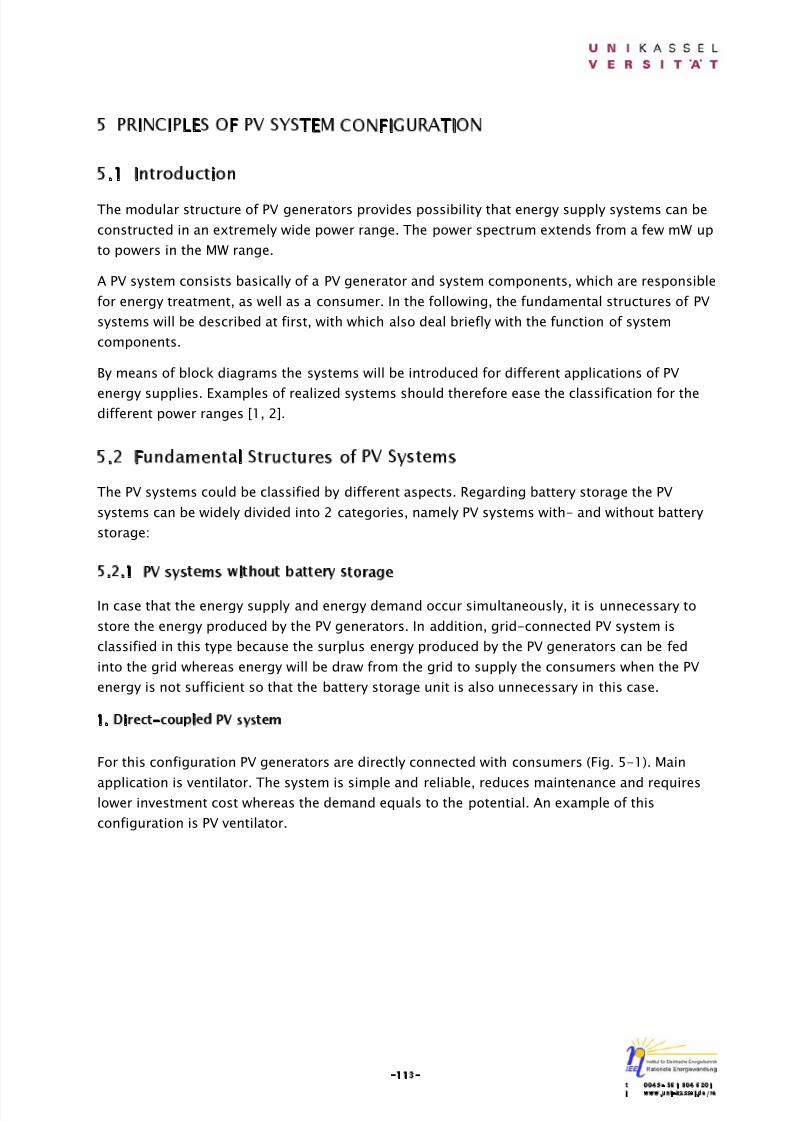
8/14/2019 Photovoltaic Systems Technology SS 2003
http://slidepdf.com/reader/full/photovoltaic-systems-technology-ss-2003 117/155
-113-t 0049- 561 804 6201i www.uni-kassel.de/re
5 PRINCIPLES OF PV SYSTEM CONFIGURATION
5.1 Introduction
The modular structure of PV generators provides possibility that energy supply systems can be
constructed in an extremely wide power range. The power spectrum extends from a few mW up
to powers in the MW range.
A PV system consists basically of a PV generator and system components, which are responsible
for energy treatment, as well as a consumer. In the following, the fundamental structures of PV
systems will be described at first, with which also deal briefly with the function of system
components.
By means of block diagrams the systems will be introduced for different applications of PV
energy supplies. Examples of realized systems should therefore ease the classification for thedifferent power ranges [1, 2].
5.2 Fundamental Structures of PV Systems
The PV systems could be classified by different aspects. Regarding battery storage the PV
systems can be widely divided into 2 categories, namely PV systems with- and without battery
storage:
5.2.1 PV systems without battery storage
In case that the energy supply and energy demand occur simultaneously, it is unnecessary to
store the energy produced by the PV generators. In addition, grid-connected PV system is
classified in this type because the surplus energy produced by the PV generators can be fed
into the grid whereas energy will be draw from the grid to supply the consumers when the PV
energy is not sufficient so that the battery storage unit is also unnecessary in this case.
1. Direct-coupled PV system
For this configuration PV generators are directly connected with consumers (Fig. 5-1). Main
application is ventilator. The system is simple and reliable, reduces maintenance and requireslower investment cost whereas the demand equals to the potential. An example of this
configuration is PV ventilator.
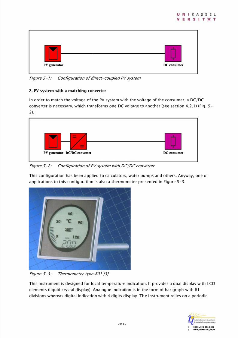
8/14/2019 Photovoltaic Systems Technology SS 2003
http://slidepdf.com/reader/full/photovoltaic-systems-technology-ss-2003 118/155
-114-t 0049- 561 804 6201i www.uni-kassel.de/re
Figure 5-1: Configuration of direct-coupled PV system
2. PV system with a matching converter
In order to match the voltage of the PV system with the voltage of the consumer, a DC/DC
converter is necessary, which transforms one DC voltage to another (see section 4.2.1) (Fig. 5-
2).
Figure 5-2: Configuration of PV system with DC/DC converter
This configuration has been applied to calculators, water pumps and others. Anyway, one of applications to this configuration is also a thermometer presented in Figure 5-3.
Figure 5-3: Thermometer type 801 [3]
This instrument is designed for local temperature indication. It provides a dual display with LCD
elements (liquid crystal display). Analogue indication is in the form of bar graph with 61
divisions whereas digital indication with 4 digits display. The instrument relies on a periodic
DC consumerPV generator DC/DC converter DC consumerPV generator DC/DC converter
DC consumerPV generator DC consumerPV generator
8/14/2019 Photovoltaic Systems Technology SS 2003
http://slidepdf.com/reader/full/photovoltaic-systems-technology-ss-2003 119/155
-115-t 0049- 561 804 6201i www.uni-kassel.de/re
measurement process with 3 seconds cycle time so that the viewer can take a current reading
even in passing. [3].
3. PV powered AC system
With the help of an inverter, which converts DC power into AC power (see section 4.6), ACconsumers can be supplied with solar energy (Fig. 5-4). This kind of system is often used for
water pumping above a certain power range (approx. 2 kW) [1].
Figure 5-4: Configuration of PV powered AC system
Figure 5-5 shows a PV pumping system for a village in Cardeiros, Brazil as an application of
this configuration. Although water demand tends to be roughly constant throughout the year, it
is very desirable to incorporate a covered storage tank in the system for using during periods of
low irradiation or pump breakdown.
Figure 5-5: PV pumping system for a village in Cardeiros, Brazil (Photo: Kassel University)
4. Grid-connected PV system
PV systems can also be connected to the public grid by means of suitable inverters (Fig. 5-6).
As mentioned before, energy storage is not necessary in this case. On sunny days the PVgenerator provides power e.g. for the electrical appliances in a house. Surplus energy is fed into
AC consumerPV generator
∼Inverter AC consumerPV generator
∼Inverter
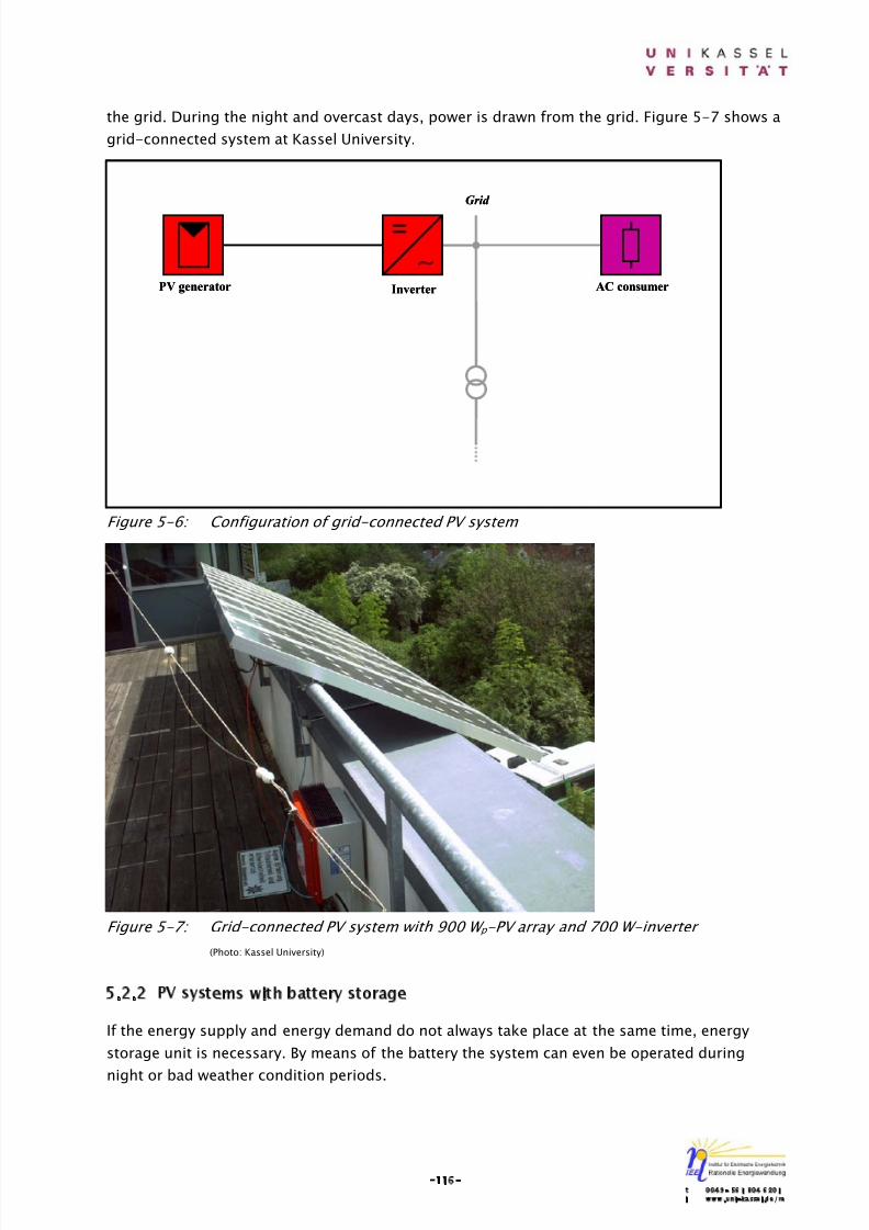
8/14/2019 Photovoltaic Systems Technology SS 2003
http://slidepdf.com/reader/full/photovoltaic-systems-technology-ss-2003 120/155
-116-t 0049- 561 804 6201i www.uni-kassel.de/re
the grid. During the night and overcast days, power is drawn from the grid. Figure 5-7 shows a
grid-connected system at Kassel University.
Figure 5-6: Configuration of grid-connected PV system
Figure 5-7: Grid-connected PV system with 900 W p -PV array and 700 W-inverter
(Photo: Kassel University)
5.2.2 PV systems with battery storage
If the energy supply and energy demand do not always take place at the same time, energy
storage unit is necessary. By means of the battery the system can even be operated during
night or bad weather condition periods.
AC consumer
Grid
∼InverterPV generator AC consumer
Grid
∼InverterPV generator
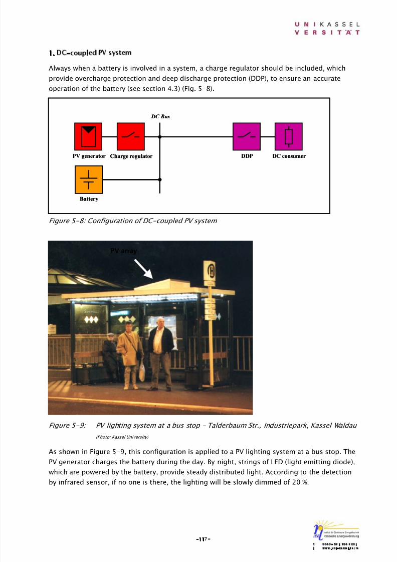
8/14/2019 Photovoltaic Systems Technology SS 2003
http://slidepdf.com/reader/full/photovoltaic-systems-technology-ss-2003 121/155
-117-t 0049- 561 804 6201i www.uni-kassel.de/re
1. DC-coupled PV system
Always when a battery is involved in a system, a charge regulator should be included, which
provide overcharge protection and deep discharge protection (DDP), to ensure an accurate
operation of the battery (see section 4.3) (Fig. 5-8).
Figure 5-8: Configuration of DC-coupled PV system
Figure 5-9: PV lighting system at a bus stop – Talderbaum Str., Industriepark, Kassel Waldau
(Photo: Kassel University)
As shown in Figure 5-9, this configuration is applied to a PV lighting system at a bus stop. The
PV generator charges the battery during the day. By night, strings of LED (light emitting diode),
which are powered by the battery, provide steady distributed light. According to the detection
by infrared sensor, if no one is there, the lighting will be slowly dimmed of 20 %.
PV array
DDP DC consumerPV generator Charge regulator
Battery
DC Bus
DDP DC consumerPV generator Charge regulator
Battery
DC Bus
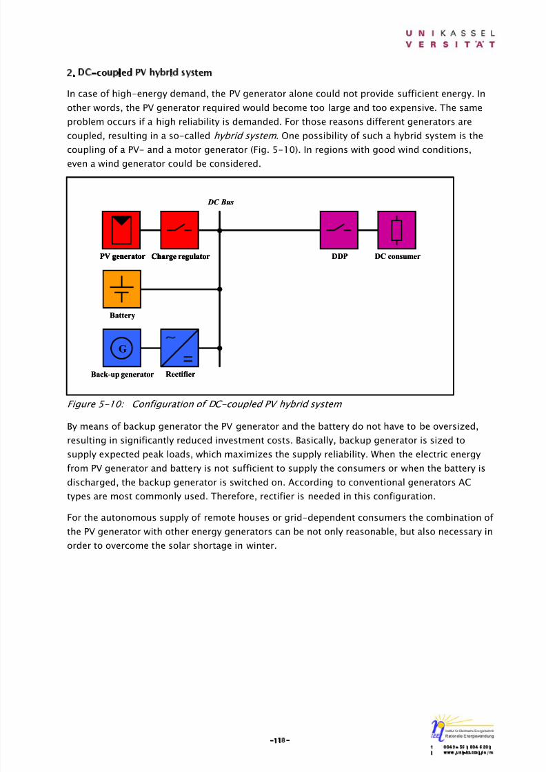
8/14/2019 Photovoltaic Systems Technology SS 2003
http://slidepdf.com/reader/full/photovoltaic-systems-technology-ss-2003 122/155
-118-t 0049- 561 804 6201i www.uni-kassel.de/re
2. DC-coupled PV hybrid system
In case of high-energy demand, the PV generator alone could not provide sufficient energy. In
other words, the PV generator required would become too large and too expensive. The same
problem occurs if a high reliability is demanded. For those reasons different generators are
coupled, resulting in a so-called hybrid system . One possibility of such a hybrid system is thecoupling of a PV- and a motor generator (Fig. 5-10). In regions with good wind conditions,
even a wind generator could be considered.
Figure 5-10: Configuration of DC-coupled PV hybrid system
By means of backup generator the PV generator and the battery do not have to be oversized,
resulting in significantly reduced investment costs. Basically, backup generator is sized to
supply expected peak loads, which maximizes the supply reliability. When the electric energy
from PV generator and battery is not sufficient to supply the consumers or when the battery is
discharged, the backup generator is switched on. According to conventional generators AC
types are most commonly used. Therefore, rectifier is needed in this configuration.
For the autonomous supply of remote houses or grid-dependent consumers the combination of
the PV generator with other energy generators can be not only reasonable, but also necessary in
order to overcome the solar shortage in winter.
PV generator Charge regulator
Battery
Back-up generator Rectifier
G
DC Bus
∼
PV generator Charge regulator DDP DC consumerPV generator Charge regulator
Battery
Back-up generator Rectifier
G
DC Bus
∼
PV generator Charge regulator DDP DC consumer
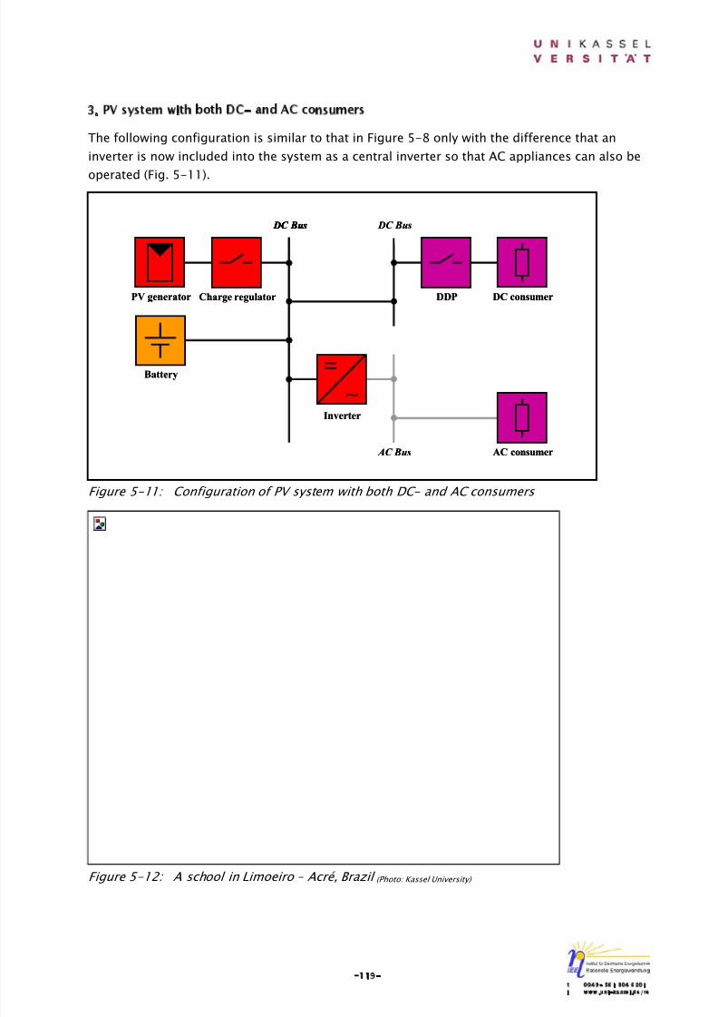
8/14/2019 Photovoltaic Systems Technology SS 2003
http://slidepdf.com/reader/full/photovoltaic-systems-technology-ss-2003 123/155
-119-t 0049- 561 804 6201i www.uni-kassel.de/re
3. PV system with both DC- and AC consumers
The following configuration is similar to that in Figure 5-8 only with the difference that an
inverter is now included into the system as a central inverter so that AC appliances can also be
operated (Fig. 5-11).
Figure 5-11: Configuration of PV system with both DC- and AC consumers
Figure 5-12: A school in Limoeiro – Acré, Brazil (Photo: Kassel University)
∼Inverter
AC consumer
DC Bus
PV generator Charge regulator
Battery
DC Bus
DDP DC consumer
DC Bus
AC Bus
∼Inverter
AC consumer
DC Bus
PV generator Charge regulator
Battery
DC Bus
DDP DC consumer
DC Bus
AC Bus
8/14/2019 Photovoltaic Systems Technology SS 2003
http://slidepdf.com/reader/full/photovoltaic-systems-technology-ss-2003 124/155
-120-t 0049- 561 804 6201i www.uni-kassel.de/re
As shown in Figure 5-12, a school in Limoeiro, Brazil, which is composed of 2 classrooms and 1
kitchen with applainces as follows: 360 W DC lighting, one satellite – for each classroom, one
television and one video player, is supplied by a PV system consisting of 660 Wp-PV array, 5
kWh-battery and 1 kW-inverter.
4. PV hybrid system with both DC- and AC consumers
The following configuration is similar to that in Figure 5-10 only with the difference that an
inverter is now included into the system as a central inverter so that AC appliances can also be
operated (Fig. 5-13).
Figure 5-13: Configuration of PV hybrid system with both DC- and AC consumers
With favourable solar radiation the consumer’s total energy demand is covered by the PV
generator. Surplus energy is stored in batteries. During the night or unfavourable weather the
energy demand is covered by the batteries at first. If deep discharge tends to occur, a diesel- or
gas-fuelled generator produces the electricity and charges the battery at the same time. At
windy sites the system can also be extended with a wind energy converter. Since PV generator
and wind energy converter can complement each other with correct design, the operating time
of the fossil-fuelled generator and thus the fuel consumption are reduced [1, 2].
This configuration can be found, for example, in the Autonomous Renewable Energy Plant
(AREP) (Fig. 5-14), a project supported by EU, which was begun at the Karlsruhe University and
carried out at the Kassel University under the direction of Prof. Dr.-Ing. Jürgen Schmid. An
objective of this project was a development of an innovative Photovoltaic/Wind hybrid system
for rural electrification, which consists of PV generator (1.6 kWp), Wind generator (0.75 kW),
battery (20 kWh) und motor generator (3 kVA) [4].
∼Inverter
AC consumer
DC Bus
PV generator Charge regulator
Battery
DC Bus
DDP DC consumer
DC Bus
AC BusBack-up generator Rectifier
G∼ ∼
Inverter
AC consumer
DC Bus
PV generator Charge regulator
Battery
DC Bus
DDP DC consumer
DC Bus
AC BusBack-up generator Rectifier
G∼
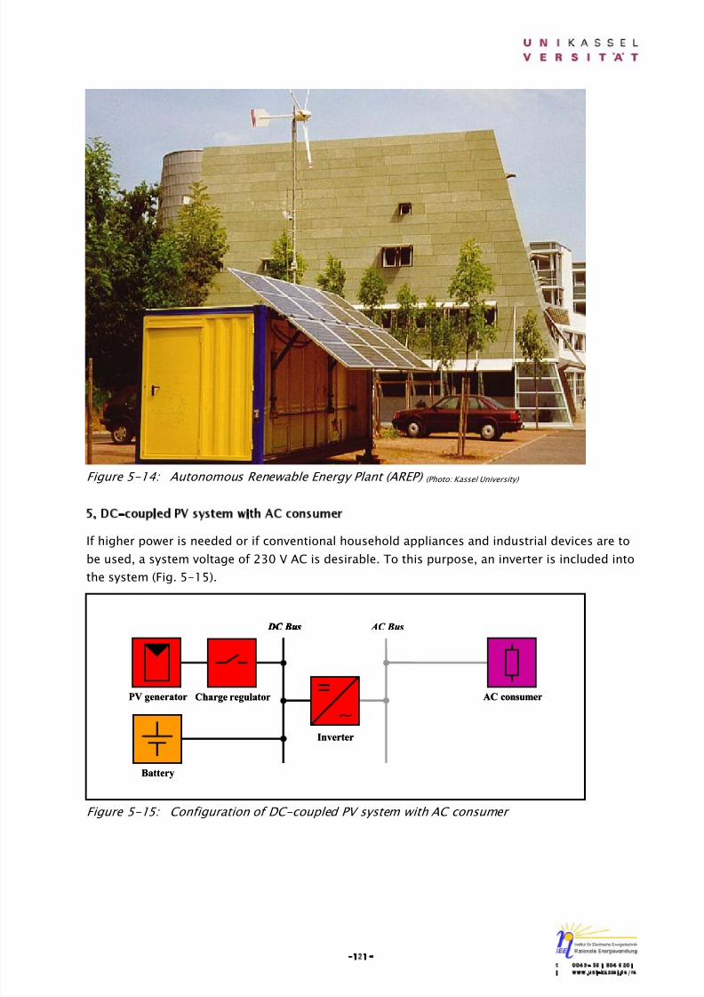
8/14/2019 Photovoltaic Systems Technology SS 2003
http://slidepdf.com/reader/full/photovoltaic-systems-technology-ss-2003 125/155
-121-t 0049- 561 804 6201i www.uni-kassel.de/re
Figure 5-14: Autonomous Renewable Energy Plant (AREP) (Photo: Kassel University)
5. DC-coupled PV system with AC consumer
If higher power is needed or if conventional household appliances and industrial devices are to
be used, a system voltage of 230 V AC is desirable. To this purpose, an inverter is included into
the system (Fig. 5-15).
Figure 5-15: Configuration of DC-coupled PV system with AC consumer
DC Bus
AC consumer
DC Bus AC Bus
∼Inverter
PV generator Charge regulator
Battery
DC Bus
AC consumer
DC Bus AC Bus
∼Inverter
PV generator Charge regulator
Battery
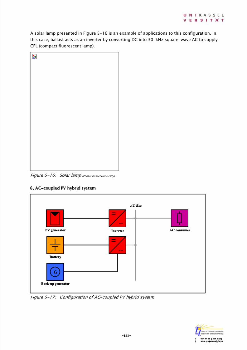
8/14/2019 Photovoltaic Systems Technology SS 2003
http://slidepdf.com/reader/full/photovoltaic-systems-technology-ss-2003 126/155
-122-t 0049- 561 804 6201i www.uni-kassel.de/re
A solar lamp presented in Figure 5-16 is an example of applications to this configuration. In
this case, ballast acts as an inverter by converting DC into 30-kHz square-wave AC to supply
CFL (compact fluorescent lamp).
Figure 5-16: Solar lamp (Photo: Kassel University)
6. AC-coupled PV hybrid system
Figure 5-17: Configuration of AC-coupled PV hybrid system
AC consumer
G
AC Bus
∼Inverter
∼
Back-up generator
PV generator
Battery
AC consumer
G
AC Bus
∼Inverter
∼
Back-up generator
PV generator
Battery
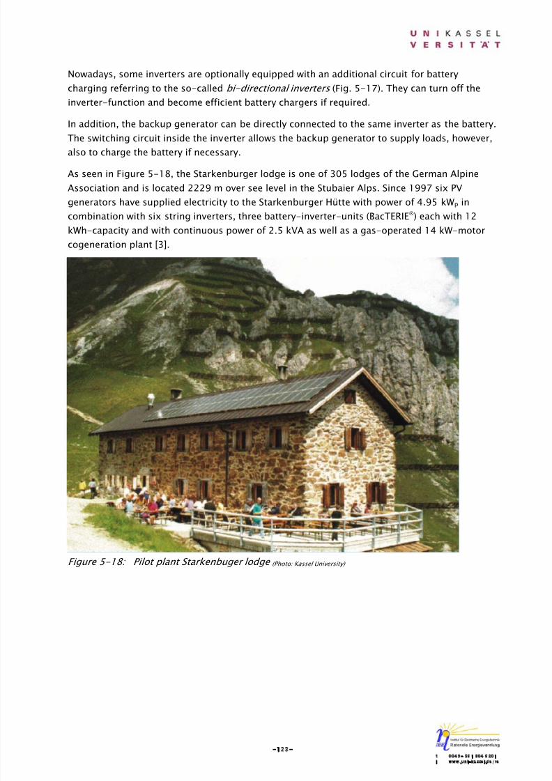
8/14/2019 Photovoltaic Systems Technology SS 2003
http://slidepdf.com/reader/full/photovoltaic-systems-technology-ss-2003 127/155
-123-t 0049- 561 804 6201i www.uni-kassel.de/re
Nowadays, some inverters are optionally equipped with an additional circuit for battery
charging referring to the so-called bi-directional inverters (Fig. 5-17). They can turn off the
inverter-function and become efficient battery chargers if required.
In addition, the backup generator can be directly connected to the same inverter as the battery.
The switching circuit inside the inverter allows the backup generator to supply loads, however,also to charge the battery if necessary.
As seen in Figure 5-18, the Starkenburger lodge is one of 305 lodges of the German Alpine
Association and is located 2229 m over see level in the Stubaier Alps. Since 1997 six PV
generators have supplied electricity to the Starkenburger Hütte with power of 4.95 kWp in
combination with six string inverters, three battery-inverter-units (BacTERIE) each with 12
kWh-capacity and with continuous power of 2.5 kVA as well as a gas-operated 14 kW-motor
cogeneration plant [3].
Figure 5-18: Pilot plant Starkenbuger lodge (Photo: Kassel University)
8/14/2019 Photovoltaic Systems Technology SS 2003
http://slidepdf.com/reader/full/photovoltaic-systems-technology-ss-2003 128/155
-124-t 0049- 561 804 6201i www.uni-kassel.de/re
5.3 Future Trends of PV Systems
Photovoltaics provide an extreme wide range of power. The presented examples show that it is
possible in many cases to replace conventional energy supply systems with a PV power supply.
Advantages, e.g. easy handling, low maintenance costs and less use of batteries, provide
further arguments for photovoltaics in photovoltaically powered appliance section.
In addition, in case of grid-dependent PV systems, PV generators can be coupled with other
power supplies, especially in areas where solar radiation fluctuates strongly. In spite of higher
costs, photovoltaics is often more economical than laying grid connection.
The applications of photovoltaics will increase both for small-decentralized power supplies and
for larger power stations. This makes a significant energy contribution. The rate of this
progress will depend on the amount of expert knowledge contributed by those involved in the
planning, construction and operation of PV systems [1, 2].
5.4 References
[1] Roth, W.: Principles of System Configuration and Application Potential .
In: Fraunhofer Institute for Solar Energy Systems: Course book for the seminar: PV
Systems; Freiburg, 1995. pg. 1-42.
[2] Roth, W.: Prinzipieller Aufbau photovoltaischer Energieversorgungssysteme .
In: Schmid, J. : Photovoltaik: Strom aus der Sonne; Technologie, Wirtschaftlichkeit und
Marktentwicklung; Heiderberg: Müller, 1999. pg. 108-116.
[3] Institut für Solare Energieversorgungstechnik: Jahresbericht 1998 , Kassel
[4] Dach, M.: Konzipierung eines Meßsystems zur energetischen Analyse von AC- und DC-
Kopplung des PV-Generators bei Hybridsystemen . Diplomarbeit; Kassel, 2001. pg. 29-
30.
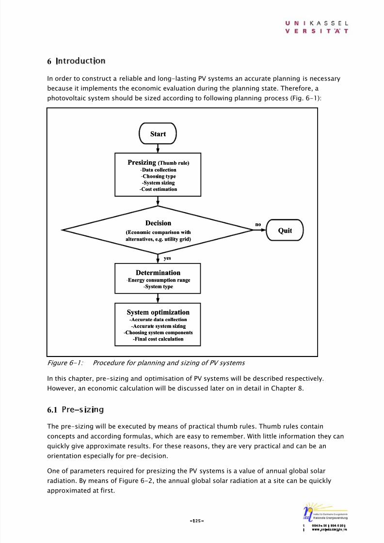
8/14/2019 Photovoltaic Systems Technology SS 2003
http://slidepdf.com/reader/full/photovoltaic-systems-technology-ss-2003 129/155
-125-t 0049- 561 804 6201i www.uni-kassel.de/re
6 Introduction
In order to construct a reliable and long-lasting PV systems an accurate planning is necessary
because it implements the economic evaluation during the planning state. Therefore, a
photovoltaic system should be sized according to following planning process (Fig. 6-1):
Figure 6-1: Procedure for planning and sizing of PV systems
In this chapter, pre-sizing and optimisation of PV systems will be described respectively.However, an economic calculation will be discussed later on in detail in Chapter 8.
6.1 Pre-sizing
The pre-sizing will be executed by means of practical thumb rules. Thumb rules contain
concepts and according formulas, which are easy to remember. With little information they can
quickly give approximate results. For these reasons, they are very practical and can be an
orientation especially for pre-decision.
One of parameters required for presizing the PV systems is a value of annual global solar
radiation. By means of Figure 6-2, the annual global solar radiation at a site can be quickly
approximated at first.
Presizing (Thumb rule)
-Data collection
-Choosing type
-System sizing
-Cost estimation
Decision
(Economic comparison with
alternatives, e.g. utility grid)
Start
yes
no
System optimization-Accurate data collection
-Accurate system sizing
-Choosing system components
-Final cost calculation
Quit
Determination-Energy consumption range
-System type
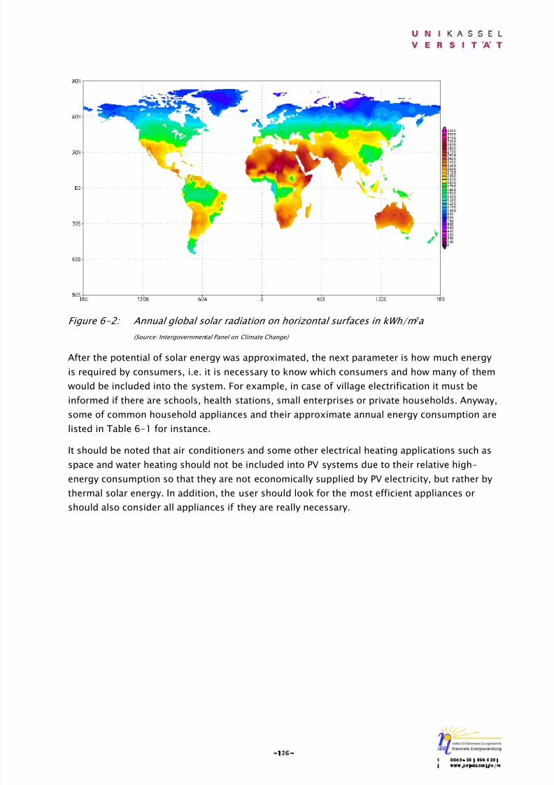
8/14/2019 Photovoltaic Systems Technology SS 2003
http://slidepdf.com/reader/full/photovoltaic-systems-technology-ss-2003 130/155
-126-t 0049- 561 804 6201i www.uni-kassel.de/re
Figure 6-2: Annual global solar radiation on horizontal surfaces in kWh/m 2 a
(Source: Intergovernmental Panel on Climate Change)
After the potential of solar energy was approximated, the next parameter is how much energy
is required by consumers, i.e. it is necessary to know which consumers and how many of them
would be included into the system. For example, in case of village electrification it must be
informed if there are schools, health stations, small enterprises or private households. Anyway,
some of common household appliances and their approximate annual energy consumption arelisted in Table 6-1 for instance.
It should be noted that air conditioners and some other electrical heating applications such as
space and water heating should not be included into PV systems due to their relative high-
energy consumption so that they are not economically supplied by PV electricity, but rather by
thermal solar energy. In addition, the user should look for the most efficient appliances or
should also consider all appliances if they are really necessary.
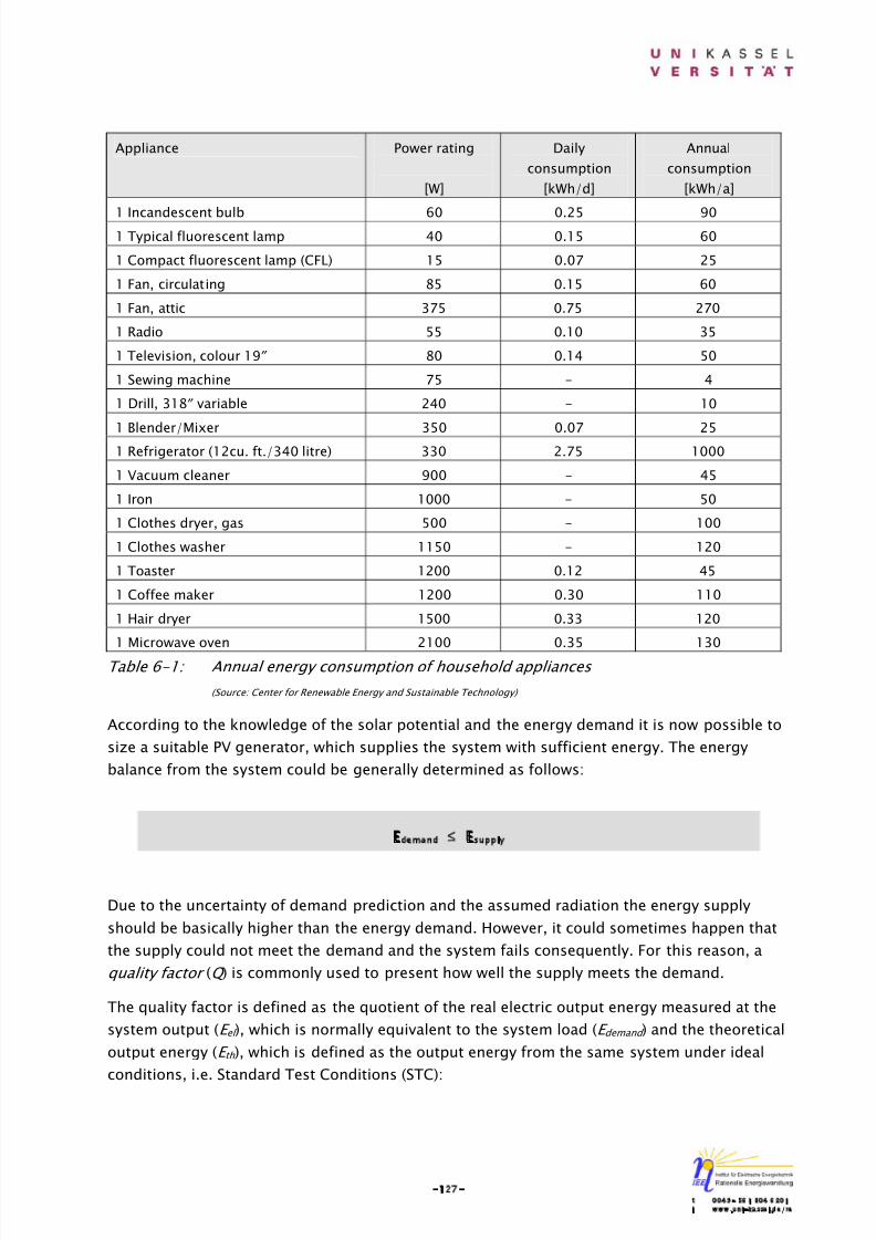
8/14/2019 Photovoltaic Systems Technology SS 2003
http://slidepdf.com/reader/full/photovoltaic-systems-technology-ss-2003 131/155
-127-t 0049- 561 804 6201i www.uni-kassel.de/re
Appliance Power rating
[W]
Daily
consumption
[kWh/d]
Annual
consumption
[kWh/a]
1 Incandescent bulb 60 0.25 901 Typical fluorescent lamp 40 0.15 60
1 Compact fluorescent lamp (CFL) 15 0.07 25
1 Fan, circulating 85 0.15 60
1 Fan, attic 375 0.75 270
1 Radio 55 0.10 35
1 Television, colour 19″ 80 0.14 50
1 Sewing machine 75 - 4
1 Drill, 318″ variable 240 - 10
1 Blender/Mixer 350 0.07 251 Refrigerator (12cu. ft./340 litre) 330 2.75 1000
1 Vacuum cleaner 900 - 45
1 Iron 1000 - 50
1 Clothes dryer, gas 500 - 100
1 Clothes washer 1150 - 120
1 Toaster 1200 0.12 45
1 Coffee maker 1200 0.30 110
1 Hair dryer 1500 0.33 120
1 Microwave oven 2100 0.35 130
Table 6-1: Annual energy consumption of household appliances
(Source: Center for Renewable Energy and Sustainable Technology)
According to the knowledge of the solar potential and the energy demand it is now possible to
size a suitable PV generator, which supplies the system with sufficient energy. The energy
balance from the system could be generally determined as follows:
Due to the uncertainty of demand prediction and the assumed radiation the energy supply
should be basically higher than the energy demand. However, it could sometimes happen that
the supply could not meet the demand and the system fails consequently. For this reason, a
quality factor (Q ) is commonly used to present how well the supply meets the demand.
The quality factor is defined as the quotient of the real electric output energy measured at the
system output (E el ), which is normally equivalent to the system load (E demand ) and the theoretical
output energy (E th ), which is defined as the output energy from the same system under ideal
conditions, i.e. Standard Test Conditions (STC):
Edemand ≤ Esupply
8/14/2019 Photovoltaic Systems Technology SS 2003
http://slidepdf.com/reader/full/photovoltaic-systems-technology-ss-2003 132/155
-128-t 0049- 561 804 6201i www.uni-kassel.de/re
Q =th
el
E
E (6-1)
where: Q = quality factor of the system
Eel = real electric output energy of the system [kWh]
Eth = theoretical output energy of the system [kWh]
The quality factor can be determined over any given time period. In most cases, a time period
of one year is chosen to presize PV systems.
The theoretical output energy (E th ) is defined as the energy output, which is produced by a PV
array with an area of Aarray , the global radiation E glob incident on a horizontal surface and
efficiency η determined under STC:
Eth = η⋅ Eglob⋅ Aarray (6-2)
where: Eth = theoretical output energy of the PV array [kWh]
η = efficiency of the PV array [decimal]
Eglob = global radiation on a horizontal surface [kWh/m2]
Aarray = area of the PV array [m2]
It is often difficult to obtain values like the efficiencies from manufacturers. Besides, the area of
the array is frequently unknown. However, the peak power measured under STC is normally
given (STC: I STC = 1000 W/m2; T STC = 25 °C, AM = 1.5):
Ppeak = η⋅ ISTC ⋅ Aarray (6-3)
where: Ppeak = peak power of the PV array [kWp]
η = efficiency of the PV array [decimal]
ISTC = incident global radiation under STC [1 kW/m2]
Aarray = area of the PV array [m2]
According to the equations (6-2) and (6-3) after substitution of η⋅ Aarray :
Eth =STC
glob
peak I
E P ⋅ (6-4)
According to the equations (6-1) and (6-4) the quality factor can be found out:
Q = STC
peak glob
el I P E
E ⋅
⋅(6-5)
With the quality factor formula above and the empirical quality factors of existing systems it is
easy to presize the PV array:
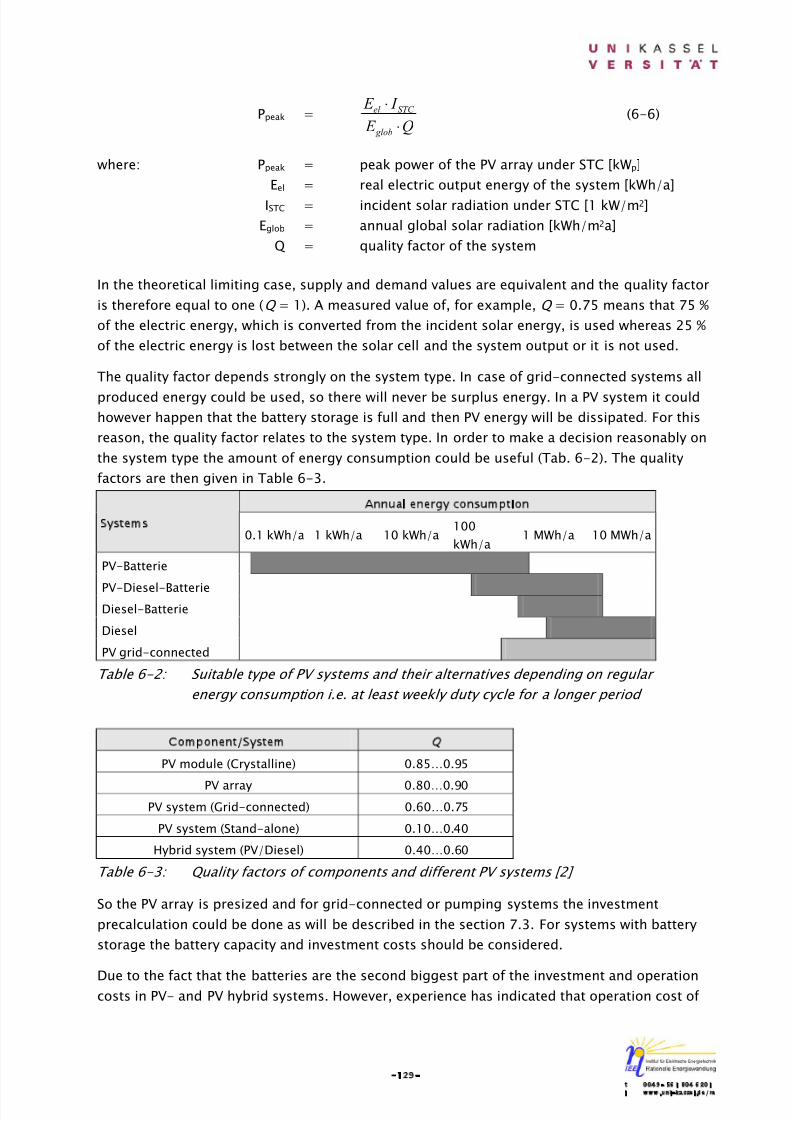
8/14/2019 Photovoltaic Systems Technology SS 2003
http://slidepdf.com/reader/full/photovoltaic-systems-technology-ss-2003 133/155
-129-t 0049- 561 804 6201i www.uni-kassel.de/re
Ppeak =Q E
I E
glob
STC el
⋅
⋅(6-6)
where: Ppeak = peak power of the PV array under STC [kWp]
Eel = real electric output energy of the system [kWh/a]
ISTC = incident solar radiation under STC [1 kW/m2]
Eglob = annual global solar radiation [kWh/m2a]
Q = quality factor of the system
In the theoretical limiting case, supply and demand values are equivalent and the quality factor
is therefore equal to one (Q = 1). A measured value of, for example, Q = 0.75 means that 75 %
of the electric energy, which is converted from the incident solar energy, is used whereas 25 %
of the electric energy is lost between the solar cell and the system output or it is not used.
The quality factor depends strongly on the system type. In case of grid-connected systems all
produced energy could be used, so there will never be surplus energy. In a PV system it couldhowever happen that the battery storage is full and then PV energy will be dissipated. For this
reason, the quality factor relates to the system type. In order to make a decision reasonably on
the system type the amount of energy consumption could be useful (Tab. 6-2). The quality
factors are then given in Table 6-3.
Annual energy consumption
Systems0.1 kWh/a 1 kWh/a 10 kWh/a
100
kWh/a1 MWh/a 10 MWh/a
PV-Batterie
PV-Diesel-BatterieDiesel-Batterie
Diesel
PV grid-connected
Table 6-2: Suitable type of PV systems and their alternatives depending on regular
energy consumption i.e. at least weekly duty cycle for a longer period
Component/System Q
PV module (Crystalline) 0.85…0.95
PV array 0.80…0.90
PV system (Grid-connected) 0.60…0.75
PV system (Stand-alone) 0.10…0.40
Hybrid system (PV/Diesel) 0.40…0.60
Table 6-3: Quality factors of components and different PV systems [2]
So the PV array is presized and for grid-connected or pumping systems the investment
precalculation could be done as will be described in the section 7.3. For systems with battery
storage the battery capacity and investment costs should be considered.
Due to the fact that the batteries are the second biggest part of the investment and operationcosts in PV- and PV hybrid systems. However, experience has indicated that operation cost of
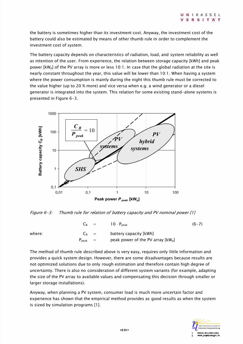
8/14/2019 Photovoltaic Systems Technology SS 2003
http://slidepdf.com/reader/full/photovoltaic-systems-technology-ss-2003 134/155
-130-t 0049- 561 804 6201i www.uni-kassel.de/re
the battery is sometimes higher than its investment cost. Anyway, the investment cost of the
battery could also be estimated by means of other thumb rule in order to complement the
investment cost of system.
The battery capacity depends on characteristics of radiation, load, and system reliability as well
as intention of the user. From experience, the relation between storage capacity [kWh] and peakpower [kWp] of the PV array is more or less 10:1. In case that the global radiation at the site is
nearly constant throughout the year, this value will be lower than 10:1. When having a system
where the power consumption is mainly during the night this thumb rule must be corrected to
the value higher (up to 20 % more) and vice versa when e.g. a wind generator or a diesel
generator is integrated into the system. This relation for some existing stand-alone systems is
presented in Figure 6-3.
Figure 6-3: Thumb rule for relation of battery capacity and PV nominal power [1]
CB = 10 ⋅ Ppeak (6-7)
where: CB = battery capacity [kWh]
Ppeak = peak power of the PV array [kWp]
The method of thumb rule described above is very easy, requires only little information and
provides a quick system design. However, there are some disadvantages because results are
not optimized solutions due to only rough estimation and therefore contain high degree of
uncertainty. There is also no consideration of different system variants (for example, adapting
the size of the PV array to available values and compensating this decision through smaller or
larger storage installations).
Anyway, when planning a PV system, consumer load is much more uncertain factor and
experience has shown that the empirical method provides as good results as when the system
is sized by simulation programs [1].
0,1
1
10
100
1000
0,01 0,1 1 10 100
Peak power P peak [kWp]
B a t t e r y c a p a c i t y C B
[ k W h ]
PV
systems
C B
P peak
= 10
SHS
PV
hybrid
systems

8/14/2019 Photovoltaic Systems Technology SS 2003
http://slidepdf.com/reader/full/photovoltaic-systems-technology-ss-2003 135/155
-131-t 0049- 561 804 6201i www.uni-kassel.de/re
6.2 Approximation of the System Cost
A factor, which strongly influences the user’s decision to invest in the system, is the system
cost. According to the fact that most users have no idea about this cost. In order to give the
user an imagination about this, overall investment cost should be precalculated by means of the
factor relating to the specific cost of PV module from experience:
KPV = kPV ⋅ Ppeak (6-8)
where: KPV = absolute cost of the PV array [€]
kPV = specific cost of the PV module [€/kWp]
Ppeak = peak power of the PV array [kWp]
The factor k PV depends on the individual country, for example, the value for Germany (2002) is
about 4.0…4.5 €/kWp.
In consequence, with the help of a factor of system components, an absolute cost of the system
can be now calculated:
KSystem = f SC ⋅ KPV (6-9)
where: Ksystem = absolute cost of PV system [€]
f SC = factor of additional system components
The factor of additional system components (f SC ) depends however on the type of system as
indicated in Table 6-4.
Component/System fSC
PV system (Grid-connected) 1.20…1.40
PV system (Stand-alone) 1.80…2.40
Hybrid system (PV/Diesel) 1.60…2.20
Table 6-4: Factors of system components for different PV systems (Source: Kassel Unversity)
To show this effect a comparison of the proportion of the PV generator’s investment cost in a
PV/Diesel hybrid system and in a grid-connected system is presented in Figure 6-4.
According to Figure 6-4 it points out that PV/Diesel hybrid systems consist of morecomponents to be invested than grid-connected systems. Therefore, their proportions of PV
generator’s investment costs are smaller than that in grid-connected systems. As a result, their
values of f SC are higher (Tab. 6-4).
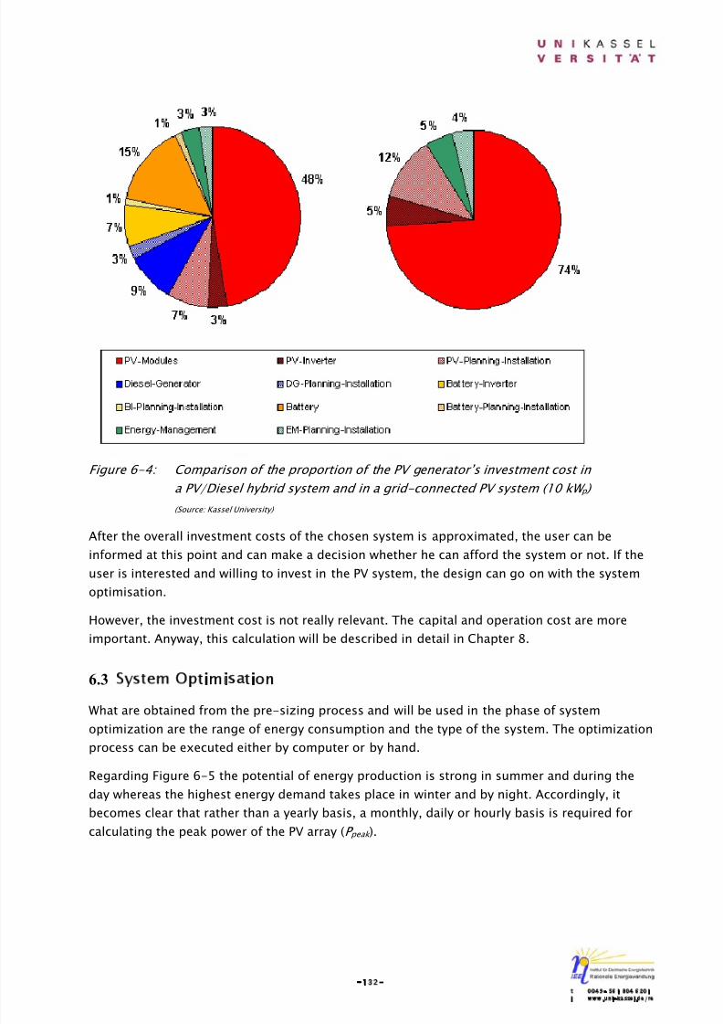
8/14/2019 Photovoltaic Systems Technology SS 2003
http://slidepdf.com/reader/full/photovoltaic-systems-technology-ss-2003 136/155
-132-t 0049- 561 804 6201i www.uni-kassel.de/re
Figure 6-4: Comparison of the proportion of the PV generator’s investment cost in
a PV/Diesel hybrid system and in a grid-connected PV system (10 kW p )
(Source: Kassel University)
After the overall investment costs of the chosen system is approximated, the user can beinformed at this point and can make a decision whether he can afford the system or not. If the
user is interested and willing to invest in the PV system, the design can go on with the system
optimisation.
However, the investment cost is not really relevant. The capital and operation cost are more
important. Anyway, this calculation will be described in detail in Chapter 8.
6.3 System Optimisation
What are obtained from the pre-sizing process and will be used in the phase of system
optimization are the range of energy consumption and the type of the system. The optimization
process can be executed either by computer or by hand.
Regarding Figure 6-5 the potential of energy production is strong in summer and during the
day whereas the highest energy demand takes place in winter and by night. Accordingly, it
becomes clear that rather than a yearly basis, a monthly, daily or hourly basis is required for
calculating the peak power of the PV array (P peak ).
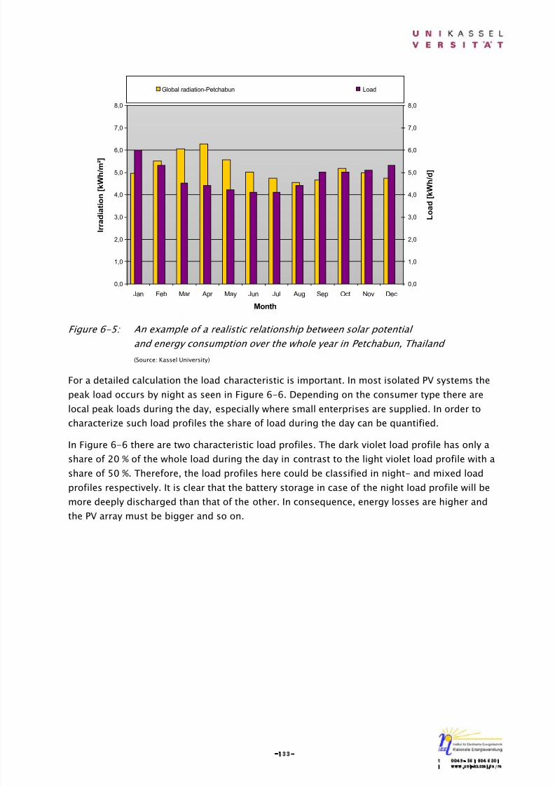
8/14/2019 Photovoltaic Systems Technology SS 2003
http://slidepdf.com/reader/full/photovoltaic-systems-technology-ss-2003 137/155
-133-t 0049- 561 804 6201i www.uni-kassel.de/re
Figure 6-5: An example of a realistic relationship between solar potential
and energy consumption over the whole year in Petchabun, Thailand
(Source: Kassel University)
For a detailed calculation the load characteristic is important. In most isolated PV systems the
peak load occurs by night as seen in Figure 6-6. Depending on the consumer type there are
local peak loads during the day, especially where small enterprises are supplied. In order tocharacterize such load profiles the share of load during the day can be quantified.
In Figure 6-6 there are two characteristic load profiles. The dark violet load profile has only a
share of 20 % of the whole load during the day in contrast to the light violet load profile with a
share of 50 %. Therefore, the load profiles here could be classified in night- and mixed load
profiles respectively. It is clear that the battery storage in case of the night load profile will be
more deeply discharged than that of the other. In consequence, energy losses are higher and
the PV array must be bigger and so on.
0,0
1,0
2,0
3,0
4,0
5,0
6,0
7,0
8,0
Jan Feb Mar Apr May Jun Jul Aug Sep Oct Nov Dec
Month
I r r a d i a t i o n [ k W h / m ² ]
0,0
1,0
2,0
3,0
4,0
5,0
6,0
7,0
8,0
L o a d [ k W h / d ]
Global radiation-Petchabun Load
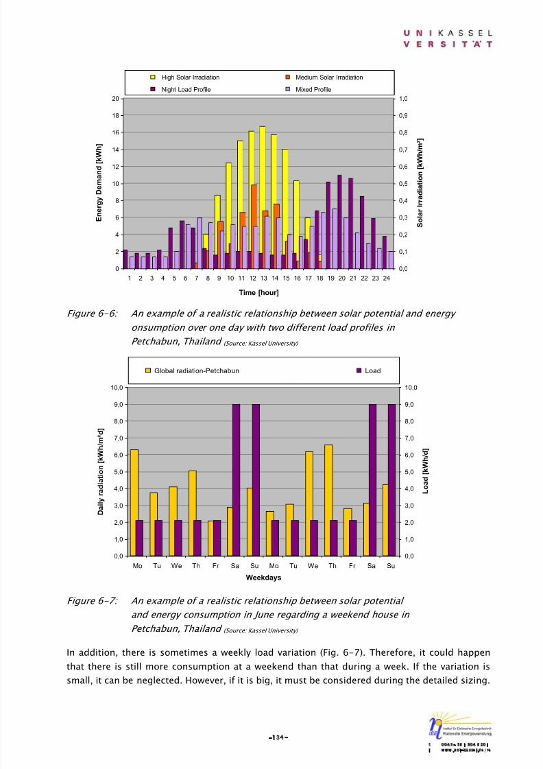
8/14/2019 Photovoltaic Systems Technology SS 2003
http://slidepdf.com/reader/full/photovoltaic-systems-technology-ss-2003 138/155
-134-t 0049- 561 804 6201i www.uni-kassel.de/re
Figure 6-6: An example of a realistic relationship between solar potential and energy
onsumption over one day with two different load profiles in
Petchabun, Thailand (Source: Kassel University)
Figure 6-7: An example of a realistic relationship between solar potential
and energy consumption in June regarding a weekend house in
Petchabun, Thailand (Source: Kassel University)
In addition, there is sometimes a weekly load variation (Fig. 6-7). Therefore, it could happen
that there is still more consumption at a weekend than that during a week. If the variation is
small, it can be neglected. However, if it is big, it must be considered during the detailed sizing.
0
2
4
6
8
10
12
14
16
18
20
1 2 3 4 5 6 7 8 9 10 11 12 13 14 15 16 17 18 19 20 21 22 23 24
Time [hour]
E n e r g y D e m a n d [ k W h ]
0,0
0,1
0,2
0,3
0,4
0,5
0,6
0,7
0,8
0,9
1,0
S o l a r I r r a d i a t i o n [ k W h / m ² ]
High Solar Irradiation Medium Solar Irradiation
Night Load Profile Mixed Profile
0,0
1,0
2,0
3,0
4,0
5,0
6,0
7,0
8,0
9,0
10,0
Mo Tu We Th Fr Sa Su Mo Tu We Th Fr Sa Su
Weekdays
D a i l y r a d i a t i o n [ k W h / m ² d ]
0,0
1,0
2,0
3,0
4,0
5,0
6,0
7,0
8,0
9,0
10,0
L o a d [ k W h / d ]
Global radiation-Petchabun Load
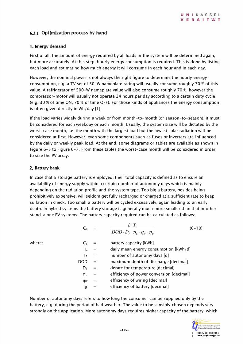
8/14/2019 Photovoltaic Systems Technology SS 2003
http://slidepdf.com/reader/full/photovoltaic-systems-technology-ss-2003 139/155
-135-t 0049- 561 804 6201i www.uni-kassel.de/re
6.3.1 Optimization process by hand
1. Energy demand
First of all, the amount of energy required by all loads in the system will be determined again,
but more accurately. At this step, hourly energy consumption is required. This is done by listing
each load and estimating how much energy it will consume in each hour and in each day.
However, the nominal power is not always the right figure to determine the hourly energy
consumption, e.g. a TV set of 50-W nameplate rating will usually consume roughly 70 % of this
value. A refrigerator of 500-W nameplate value will also consume roughly 70 %, however the
compressor-motor will usually not operate 24 hours per day according to a certain duty cycle
(e.g. 30 % of time ON, 70 % of time OFF). For those kinds of appliances the energy consumption
is often given directly in Wh/day [1].
If the load varies widely during a week or from month-to-month (or season-to-season), it must
be considered for each weekday or each month. Usually, the system size will be dictated by the
worst-case month, i.e. the month with the largest load but the lowest solar radiation will be
considered at first. However, even some components such as fuses or inverters are influenced
by the daily or weekly peak load. At the end, some diagrams or tables are available as shown in
Figure 6-5 to Figure 6-7. From these tables the worst-case month will be considered in order
to size the PV array.
2. Battery bank
In case that a storage battery is employed, their total capacity is defined as to ensure an
availability of energy supply within a certain number of autonomy days which is mainly
depending on the radiation profile and the system type. Too big a battery, besides being
prohibitively expensive, will seldom get fully recharged or charged at a sufficient rate to keep
sulfation in check. Too small a battery will be cycled excessively, again leading to an early
death. In hybrid systems the battery storage is generally much more smaller than that in other
stand-alone PV systems. The battery capacity required can be calculated as follows:
CB = BW C T
A
D DOD
T L
η η η ⋅⋅⋅⋅
⋅(6-10)
where: CB = battery capacity [kWh]
L = daily mean energy consumption [kWh/d]
TA = number of autonomy days [d]
DOD = maximum depth of discharge [decimal]
DT = derate for temperature [decimal]
ηC = efficiency of power conversion [decimal]
ηW = efficiency of wiring [decimal]
ηB = efficiency of battery [decimal]
Number of autonomy days refers to how long the consumer can be supplied only by the
battery, e.g. during the period of bad weather. The value to be sensibly chosen depends very
strongly on the application. More autonomy days requires higher capacity of the battery, which
8/14/2019 Photovoltaic Systems Technology SS 2003
http://slidepdf.com/reader/full/photovoltaic-systems-technology-ss-2003 140/155
-136-t 0049- 561 804 6201i www.uni-kassel.de/re
provides higher supply reliability. The maximum depth of discharge refers to how many percent
of battery capacity are usable in practice (see section 4.3.4).
If the battery will be operated with below 20 °C operating temperature, its capacity will be
reduced. Therefore, a factor that derates the battery capacity for cold operating temperatures is
taken into consideration. If no better information is available, derate a lead-acid battery’scapacity one percent for each degree Celsius below 20 °C operating temperature [4].
However, the operating temperature of the battery in Thailand, for example, is often higher
than 20 °C. The battery capacity will be higher but its lifetime will be shortened. In this case the
factor D T should be assumed to be constant.
The efficiency of power conversion accounts for power loss in systems using power
conditioning components (converters or inverters). The efficiency of wiring accounts for loss
due to wiring and switchgear. This factor can vary from 0.95 to 0.99. The battery efficiency can
be obtained from manufacturer’s data for specific battery [4].
3. PV array
In order to size the PV array in an adequate manner the orientation and the tilt angle of the PV
array must be considered at first. The optimal tilt angel is depending on the latitude of the
system location. For the first assumption the tilt angel should be equivalent to the latitude.
However for the location further from the equator, the tilt angle will be smaller than the latitude
in order to obtain an optimal annual solar potential.
An example gives Figure 6-8. The annual solar potential is here given as a function of
orientation and tilt angle for Kassel. The optimum tilt angle of about 30° is smaller than thelatitude (Kassel: 51° 18 ′ N ) due to the major share of solar radiation between April and August
in the northern hemisphere.
Near of the equator a minimum of tilt angle of 15° is recommended in order to realize a self-
cleaning effect during rainfalls.
The best tilt angle for the worst-case month relates to the sun zenith of this month and could
be estimated as follow:
α ≈ 90 – z (6-11)
where: α = tilt angle [°]
z = sun zenith [°]
In addition, the equations explained above are valid in a similar manner for determination of
cable cross-section at the consumer side [2].
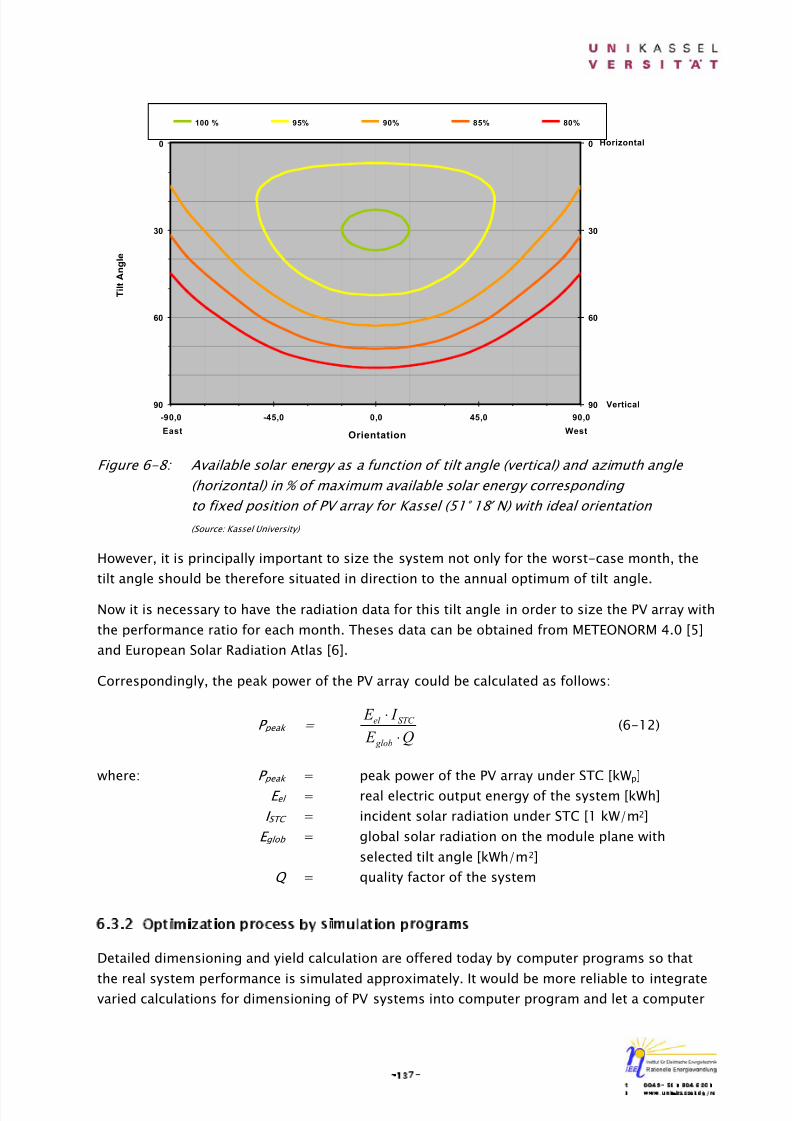
8/14/2019 Photovoltaic Systems Technology SS 2003
http://slidepdf.com/reader/full/photovoltaic-systems-technology-ss-2003 141/155
-137-t 0049- 561 804 6201i www.uni-kassel.de/re
Figure 6-8: Available solar energy as a function of tilt angle (vertical) and azimuth angle
(horizontal) in % of maximum available solar energy corresponding
to fixed position of PV array for Kassel (51° 18 ′ N) with ideal orientation
(Source: Kassel University)
However, it is principally important to size the system not only for the worst-case month, the
tilt angle should be therefore situated in direction to the annual optimum of tilt angle.
Now it is necessary to have the radiation data for this tilt angle in order to size the PV array with
the performance ratio for each month. Theses data can be obtained from METEONORM 4.0 [5]
and European Solar Radiation Atlas [6].
Correspondingly, the peak power of the PV array could be calculated as follows:
P peak = Q E
I E
glob
STC el
⋅
⋅(6-12)
where: P peak = peak power of the PV array under STC [kWp]
E el = real electric output energy of the system [kWh]
I STC = incident solar radiation under STC [1 kW/m2]
E glob = global solar radiation on the module plane with
selected tilt angle [kWh/m2]
Q = quality factor of the system
6.3.2 Optimization process by simulation programs
Detailed dimensioning and yield calculation are offered today by computer programs so that
the real system performance is simulated approximately. It would be more reliable to integratevaried calculations for dimensioning of PV systems into computer program and let a computer
0
30
60
90
-90,0 -45,0 0,0 45,0 90,0
Orientation
T i l t A n g l e
0
30
60
90
100 % 95% 90% 85% 80%
WestEast
Horizontal
Vertical
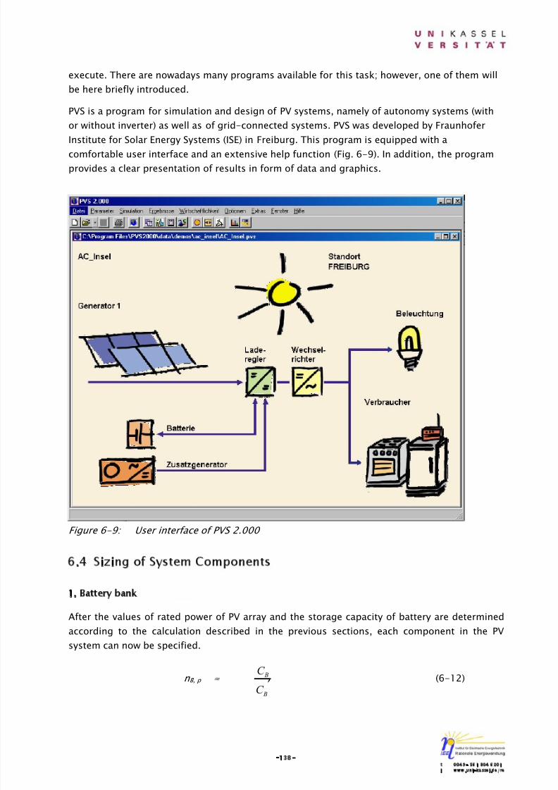
8/14/2019 Photovoltaic Systems Technology SS 2003
http://slidepdf.com/reader/full/photovoltaic-systems-technology-ss-2003 142/155
-138-t 0049- 561 804 6201i www.uni-kassel.de/re
execute. There are nowadays many programs available for this task; however, one of them will
be here briefly introduced.
PVS is a program for simulation and design of PV systems, namely of autonomy systems (with
or without inverter) as well as of grid-connected systems. PVS was developed by Fraunhofer
Institute for Solar Energy Systems (ISE) in Freiburg. This program is equipped with acomfortable user interface and an extensive help function (Fig. 6-9). In addition, the program
provides a clear presentation of results in form of data and graphics.
Figure 6-9: User interface of PVS 2.000
6.4 Sizing of System Components
1. Battery bank
After the values of rated power of PV array and the storage capacity of battery are determined
according to the calculation described in the previous sections, each component in the PV
system can now be specified.
n B, p ≈ ′
B
B
C
C (6-12)
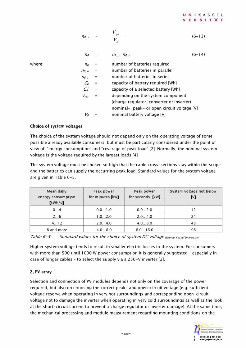
8/14/2019 Photovoltaic Systems Technology SS 2003
http://slidepdf.com/reader/full/photovoltaic-systems-technology-ss-2003 143/155
-139-t 0049- 561 804 6201i www.uni-kassel.de/re
n B, s ≈ B
sys
V
V (6-13)
n B = n B, p ⋅ n B, s (6-14)
where: n B = number of batteries required
n B, p = number of batteries in parallel
n B , s = number of batteries in series
C B = capacity of battery required [Wh]
C B ’ = capacity of a selected battery [Wh]
V sys = depending on the system component
(charge regulator, converter or inverter)
nominal-, peak- or open circuit voltage [V]
V B = nominal battery voltage [V]
Choice of system voltages
The choice of the system voltage should not depend only on the operating voltage of some
possible already available consumers, but must be particularly considered under the point of
view of “energy consumption” and “coverage of peak load” [2]. Normally, the nominal system
voltage is the voltage required by the largest loads [4]
The system voltage must be chosen so high that the cable cross-sections stay within the scope
and the batteries can supply the occurring peak load. Standard values for the system voltage
are given in Table 6-5.
Mean daily
energy consumption
[kWh/d]
Peak power
for minutes [kW]
Peak power
for seconds [kW]
System voltage not below
[V]
0…4 0.0…1.0 0.0…2.0 12
2…6 1.0…2.0 2.0…4.0 24
4…12 2.0…4.0 4.0…8.0 48
8 and more 4.0…8.0 8.0…16.0 96
Table 6-5: Standard values for the choice of system DC voltage (Source: Kassel University)
Higher system voltage tends to result in smaller electric losses in the system. For consumers
with more than 500 until 1000 W power consumption it is generally suggested – especially in
case of longer cables – to select the supply via a 230-V inverter [2].
2. PV array
Selection and connection of PV modules depends not only on the coverage of the power
required, but also on choosing the correct peak- and open-circuit voltage (e.g. sufficient
voltage reserve when operating in very hot surroundings and corresponding open-circuit
voltage not to damage the inverter when operating in very cold surroundings as well as the look
at the short-circuit current to prevent a charge regulator or inverter damage). At the same time,
the mechanical processing and module measurement regarding mounting conditions on the

8/14/2019 Photovoltaic Systems Technology SS 2003
http://slidepdf.com/reader/full/photovoltaic-systems-technology-ss-2003 144/155
-140-t 0049- 561 804 6201i www.uni-kassel.de/re
location and available place complied are also to be considered. To calculate the number of PV
modules the following relations could be used:
n PV, m ≈ m PV
a PV
P
P
,
, (6-15)
where: n PV, m = estimated number of PV modules
P PV, a = nominal power of the PV array [kW]
P PV, m = nominal power of the selected PV mudule [kW]
To calculate the number of serial connected modules the following formula could be used:
n PV, m, s ≈ m PV
sys
V
V
,
(6-16)
where: n PV, m, s = estimated number of PV modules in series
V sys = depending on the system component
(charge regulator, converter or inverter)nominal-, peak- or open circuit voltage [V]
V PV, m = nominal-, peak- or open-circuit voltage of the PV
module [V]
To calculate the number of parallel connected strings the following formula could be used:
n PV, s, p ≈ sm PV
m PV
n
n
,,
,(6-17)
where: n PV, s, p = estimated number of PV strings in paralleln PV, m = estimated number of PV modules
n PV, m, s = estimated number of PV modules serial
In case that the number calculated is not an integer it must be rounded and afterwards the PV
array power must be adapted probably.
3. Charge Regulator
The charge regulator must be able to carry the maximum current occurring at the PV generator
side and its voltage must match with the system voltage. Besides, the load disconnection at the
consumer side must be designed for the maximum current consumed by the consumers. The
battery type (Lead acid or lead gel) should be selectable. Some charge regulators known the
system voltage and adjust them self some others are selectable.
4. Inverter
The grid-connected inverter must be able to carry the maximum current occurring at the PV
array side and it must match with the maximum PV array voltage.
An uncertainty, which occasionally occurs when selecting the battery, is whether long-life, but
very expensive stationary type as lead-acid or lead-gel is preferable in comparison to cheaptype with shorter lifetime and cycling stability. If this question cannot be clearly answered with

8/14/2019 Photovoltaic Systems Technology SS 2003
http://slidepdf.com/reader/full/photovoltaic-systems-technology-ss-2003 145/155
-141-t 0049- 561 804 6201i www.uni-kassel.de/re
type and duration, the decision will be finally met by the customer. Since the customer is not
always ready to pay the high investment cost for the technically better and long-life solution
even if the sum of investment- and operation cost counted over lifetime of the system speaks
rather in the expensive system.
The selection of the stand-alone inverter will be determined especially by the AC power to beprovided and the selected DC voltage. A stand-alone inverter must be able to power all of the
loads that might run at the same time, including any starting surges for pumps and other large
motors. When looking at inverter specifications, play close attention to the part load efficiency
of the inverter. Related to the over sizing related to the peak current security the stand alone
inverter is mostly running in part load about 10 to 30 % of nominal load.
5. Cabling
Due to the fact that PV energy is very expensive all system components should be energy
efficient. The efficiency of the cabling don’t should exide 1 % and 3 % respectively [2]. Cablecross-section can be calculated as follows:
A = sysV v
I l
⋅
⋅⋅⋅ 2 ρ (6-18)
or A = 2
2
sysV v
P l
⋅
⋅⋅⋅ ρ (6-19)
where: A = cable cross-section [mm2]
ρ = specific resistance [Ω⋅mm2/m]
= 0.0179 Ω⋅mm2/m for copper
l = single cable length [m]
I = rated current through the cable [A]
v = permissible loss in the cable (e.g. 3 % → v = 0.03)
V sys = depending on the system component
(charge regulator, converter or inverter)
nominal-, peak- or open circuit voltage [V]
P = power of the PV generator or the device [W]
To calculate size of the cable cross-sections, therefore, the cable’s length of the main cable
(feed line) in the concerned application must be known approximately. The cable length (l ) is
doubled in both of equations above due to single- and return cable.
In practice, according to the value resulted from the calculation the next larger standard size is
to be chosen.
For example, cross-section of a 10-m DC main cable, which connects a 120-W PV generator
with 12-V battery and should show maximum 1 % loss, can be determined by applying (6-4):
8/14/2019 Photovoltaic Systems Technology SS 2003
http://slidepdf.com/reader/full/photovoltaic-systems-technology-ss-2003 146/155
-142-t 0049- 561 804 6201i www.uni-kassel.de/re
A = 21201.0
1201020179.0
⋅
⋅⋅⋅= 29.8 mm2
As a result, a cable with 35 mm2 will be installed. If higher loss is acceptable, a cable with 25
mm2 can be applied instead.
If the system voltage is double chosen with 24 V, the cable cross-section can be reduced to a
quarter.
A = 22401.0
1201020179.0
⋅
⋅⋅⋅= 7.46 mm2
Therefore, a next larger standard cable with 10 mm2 will be used.
In addition, the equations explained above are valid in a similar manner for determination of
cable cross-section at the consumer side [2].
6.5 References
[1] Stadler, I.: PV for the world’s villages Network to Catalyse Sustainable Large Scale
Integration of PV in Developing Countries; Final Report - Task 2; Kassel, 1996.
[2] Ladener, H.: Solare Stromversorgung: Grundlagen, Planung, Anwenddung; Freiburg:
ökobuch Verlag, 1996. pg. 153-182.
[3] Kaiser, R.: Sizing photovoltaic systems. In: Fraunhofer Institute for Solar Energy
Systems: Course book for the seminar: Photovoltaic Systems; Freiburg, 1995. pg. 403-440.
[4] Sandia National Laboratories: Stand-Alone Photovoltaic Systems: A Handbook of
Recommended Design Practices; www.sandia.gov/pv/sysd/Wkshts1-5.html, 1988.
[5] METEOTEST; Swiss Federal Office of Energy: METEONORM 4.0: Global Meteorological
Database for Solar Energy and Applied Meteorology; Bern, Switzerland.
[6] Palz, W.; Greif, J., Commission of the European Communities: Europen Solar Radiation
Atlas: Solar Radiation on Horizontal and Inclined Surfaces: Springer, 1996.
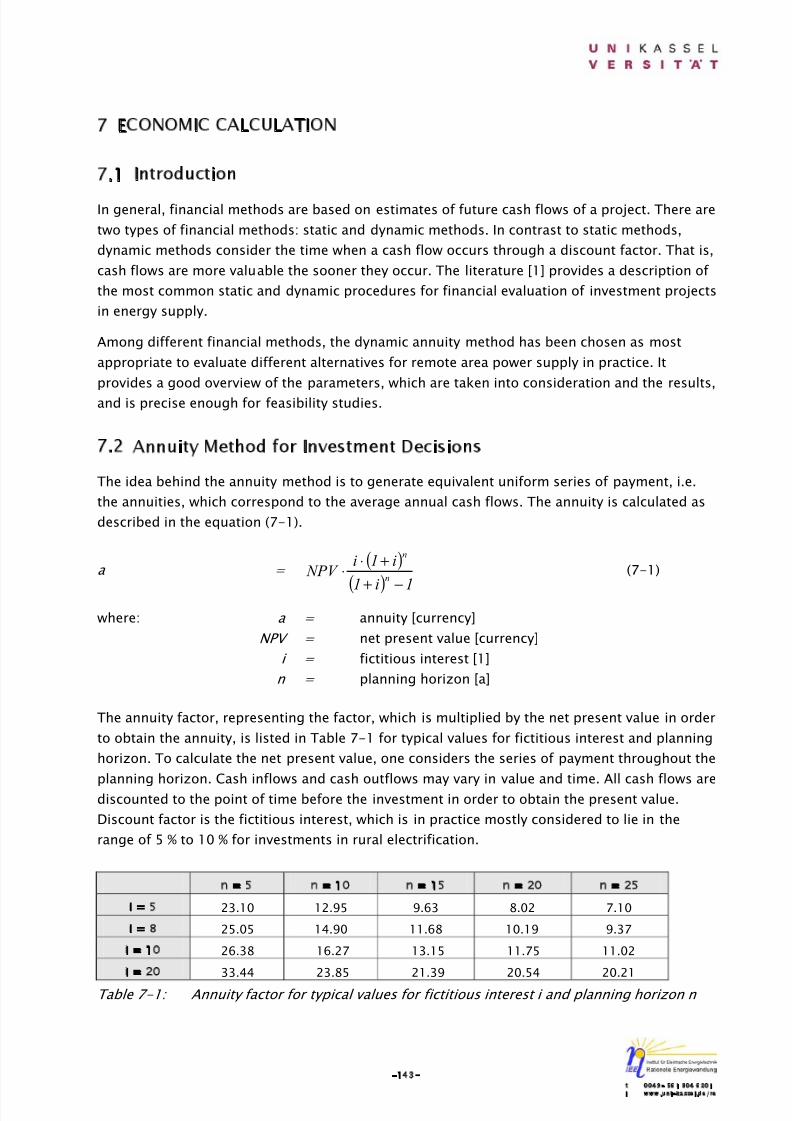
8/14/2019 Photovoltaic Systems Technology SS 2003
http://slidepdf.com/reader/full/photovoltaic-systems-technology-ss-2003 147/155
-143-t 0049- 561 804 6201i www.uni-kassel.de/re
7 ECONOMIC CALCULATION
7.1 Introduction
In general, financial methods are based on estimates of future cash flows of a project. There are
two types of financial methods: static and dynamic methods. In contrast to static methods,
dynamic methods consider the time when a cash flow occurs through a discount factor. That is,
cash flows are more valuable the sooner they occur. The literature [1] provides a description of
the most common static and dynamic procedures for financial evaluation of investment projects
in energy supply.
Among different financial methods, the dynamic annuity method has been chosen as most
appropriate to evaluate different alternatives for remote area power supply in practice. It
provides a good overview of the parameters, which are taken into consideration and the results,
and is precise enough for feasibility studies.
7.2 Annuity Method for Investment Decisions
The idea behind the annuity method is to generate equivalent uniform series of payment, i.e.
the annuities, which correspond to the average annual cash flows. The annuity is calculated as
described in the equation (7-1).
a = ( )
( ) 1i1
i1i NPV
n
n
−+
+⋅⋅ (7-1)
where: a = annuity [currency]
NPV = net present value [currency]
i = fictitious interest [1]
n = planning horizon [a]
The annuity factor, representing the factor, which is multiplied by the net present value in order
to obtain the annuity, is listed in Table 7-1 for typical values for fictitious interest and planning
horizon. To calculate the net present value, one considers the series of payment throughout the
planning horizon. Cash inflows and cash outflows may vary in value and time. All cash flows arediscounted to the point of time before the investment in order to obtain the present value.
Discount factor is the fictitious interest, which is in practice mostly considered to lie in the
range of 5 % to 10 % for investments in rural electrification.
n = 5 n = 10 n = 15 n = 20 n = 25
i = 5 23.10 12.95 9.63 8.02 7.10
i = 8 25.05 14.90 11.68 10.19 9.37
i = 10 26.38 16.27 13.15 11.75 11.02
i = 20 33.44 23.85 21.39 20.54 20.21
Table 7-1: Annuity factor for typical values for fictitious interest i and planning horizon n
8/14/2019 Photovoltaic Systems Technology SS 2003
http://slidepdf.com/reader/full/photovoltaic-systems-technology-ss-2003 148/155
-144-t 0049- 561 804 6201i www.uni-kassel.de/re
The net present value is calculated as the sum of all present values of the net cash flows as
shown in the equation (7-2).
In case that the annual cash flows remain equal, the annual net cash flow equals the annuity
and can be directly used in the annuity calculation.
For the example of photovoltaic power supply, there is often only one investment at the
beginning of the planning horizon whereas all other cash flows consist of uniform payments
such as annual fuel cost or maintenance cost. In this case, one adds the annuity of the
investment, i.e. the investment transformed into average annual cost, directly to all other
annual cost in order to obtain the overall annual cost of the project. The net present value of
the investment equals its value at the time of investment, because the investment takes place at
the beginning of the planning horizon (t = 0).
NPV = ( ) t n
0t
t i1 NCF −
=
+∑ (7-2)
where: NPV = net present value [currency]
NCF t = net cash flow at time t [currency]
t = time of cash flow
i = fictitious interest [1]
n = planning horizon [a]
7.3 Scenario Technique
Scenario technique addresses the problem that future cash flows cannot be predicted precisely
over a period of 20 years. By establishing different scenarios, it is possible to project different
future developments of relevant parameters, e.g. the fictitious interest and lifetimes of system
components.
In this work, a PV/Diesel hybrid system is designed for a village according to certain daily
energy demand. Specific energy cost of the system is then calculated by means of annuity
method. Five scenarios will be established with regard to variation of daily energy demands in
order to find out how specific energy cost depends on daily energy demand. In addition,
variation of load profiles (characteristics of load) will also be considered.
7.4 Economic Calculation for the PV/Diesel Hybrid System
The annuity method described in the previous topic will be applied to calculate the economic
efficiency of a PV-Diesel-Battery System. Values are based on a case study for a village in
Petchabun, Thailand. Result is a specific energy cost [€/kWh] generated by the system at a
given application, i.e. a given energy demand by the users and a given irradiation at the
location.
The calculation will consider investment costs for different system components with their
specific lifetimes as well as a rate for planning and installation.
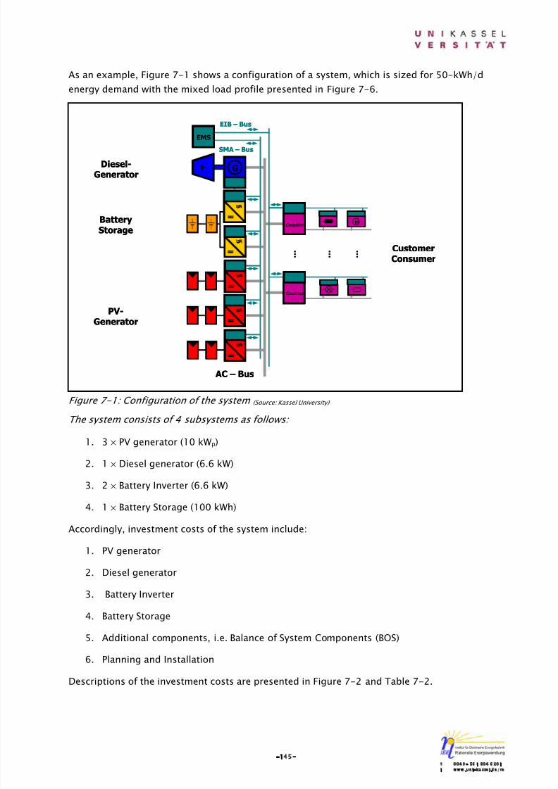
8/14/2019 Photovoltaic Systems Technology SS 2003
http://slidepdf.com/reader/full/photovoltaic-systems-technology-ss-2003 149/155
-145-t 0049- 561 804 6201i www.uni-kassel.de/re
As an example, Figure 7-1 shows a configuration of a system, which is sized for 50-kWh/d
energy demand with the mixed load profile presented in Figure 7-6.
Figure 7-1: Configuration of the system (Source: Kassel University)
The system consists of 4 subsystems as follows:
1. 3 × PV generator (10 kWp)
2. 1 × Diesel generator (6.6 kW)
3. 2 × Battery Inverter (6.6 kW)
4. 1 × Battery Storage (100 kWh)
Accordingly, investment costs of the system include:
1. PV generator
2. Diesel generator
3. Battery Inverter
4. Battery Storage
5. Additional components, i.e. Balance of System Components (BOS)
6. Planning and Installation
Descriptions of the investment costs are presented in Figure 7-2 and Table 7-2.
CustomerConsumer
Diesel-Generator
BatteryStorage
PV-Generator
Counter
CounterM
AC – Bus
EMS
G
EIB – Bus
SMA – Bus
… … … CustomerConsumer
Diesel-Generator
BatteryStorage
PV-Generator
Counter
CounterCounterMM
AC – Bus
EMSEMS
G
EIB – Bus
SMA – Bus
… … …
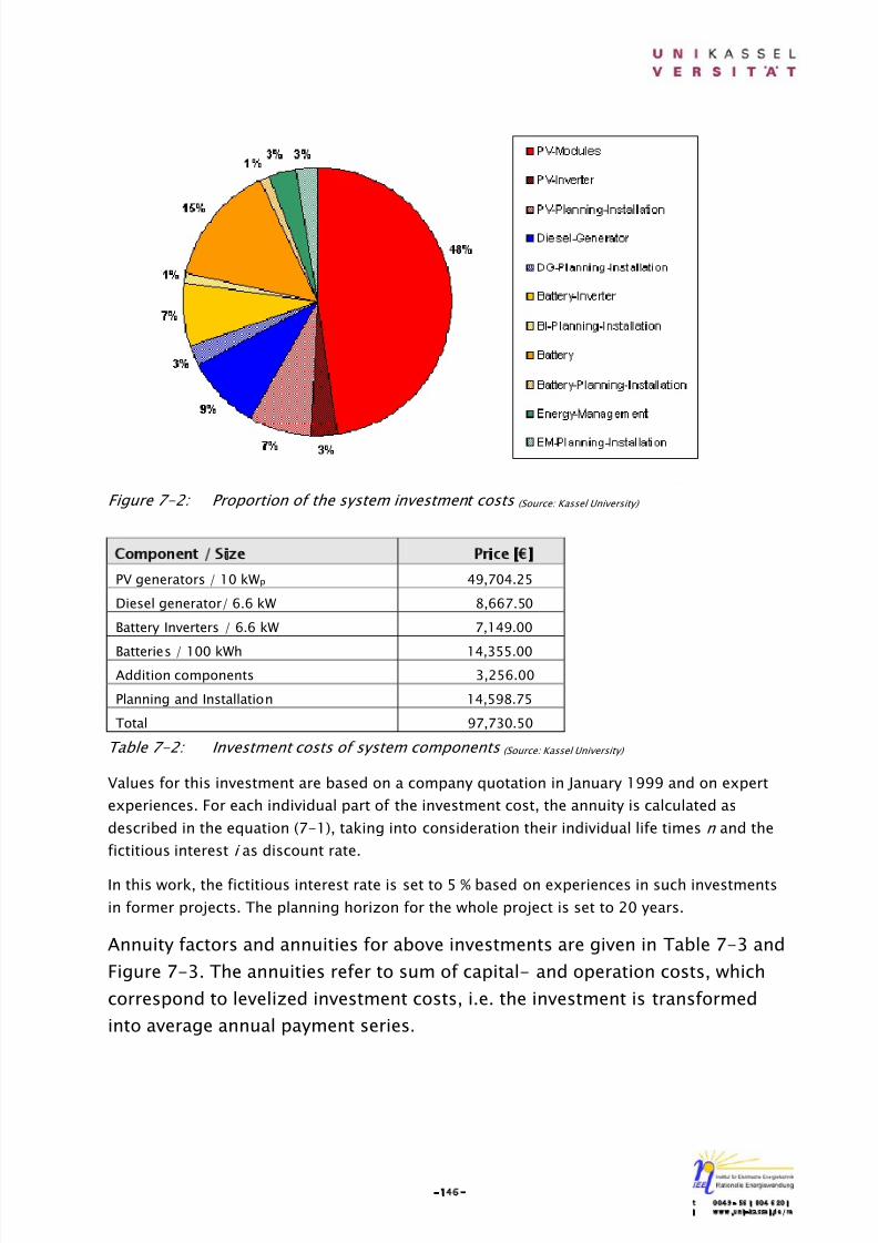
8/14/2019 Photovoltaic Systems Technology SS 2003
http://slidepdf.com/reader/full/photovoltaic-systems-technology-ss-2003 150/155
-146-t 0049- 561 804 6201i www.uni-kassel.de/re
Figure 7-2: Proportion of the system investment costs (Source: Kassel University)
Component / Size Price [€]
PV generators / 10 kWp 49,704.25
Diesel generator/ 6.6 kW 8,667.50
Battery Inverters / 6.6 kW 7,149.00
Batteries / 100 kWh 14,355.00Addition components 3,256.00
Planning and Installation 14,598.75
Total 97,730.50
Table 7-2: Investment costs of system components (Source: Kassel University)
Values for this investment are based on a company quotation in January 1999 and on expert
experiences. For each individual part of the investment cost, the annuity is calculated as
described in the equation (7-1), taking into consideration their individual life times n and the
fictitious interest i as discount rate.
In this work, the fictitious interest rate is set to 5 % based on experiences in such investments
in former projects. The planning horizon for the whole project is set to 20 years.
Annuity factors and annuities for above investments are given in Table 7-3 and
Figure 7-3. The annuities refer to sum of capital- and operation costs, which
correspond to levelized investment costs, i.e. the investment is transformed
into average annual payment series.
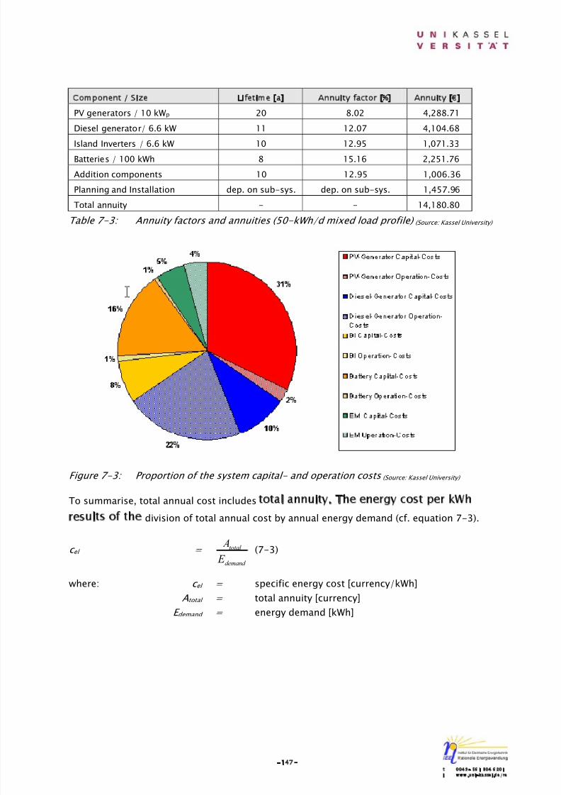
8/14/2019 Photovoltaic Systems Technology SS 2003
http://slidepdf.com/reader/full/photovoltaic-systems-technology-ss-2003 151/155
-147-t 0049- 561 804 6201i www.uni-kassel.de/re
Component / Size Lifetime [a] Annuity factor [%] Annuity [€]
PV generators / 10 kWp 20 8.02 4,288.71
Diesel generator/ 6.6 kW 11 12.07 4,104.68
Island Inverters / 6.6 kW 10 12.95 1,071.33
Batteries / 100 kWh 8 15.16 2,251.76
Addition components 10 12.95 1,006.36
Planning and Installation dep. on sub-sys. dep. on sub-sys. 1,457.96
Total annuity - - 14,180.80
Table 7-3: Annuity factors and annuities (50-kWh/d mixed load profile) (Source: Kassel University)
Figure 7-3: Proportion of the system capital- and operation costs (Source: Kassel University)
To summarise, total annual cost includes total annuity. The energy cost per kWh
results of the division of total annual cost by annual energy demand (cf. equation 7-3).
c el =
demand
total
E
A(7-3)
where: c el = specific energy cost [currency/kWh]
Atotal = total annuity [currency]
E demand = energy demand [kWh]
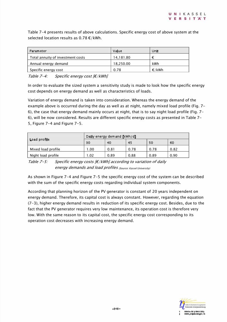
8/14/2019 Photovoltaic Systems Technology SS 2003
http://slidepdf.com/reader/full/photovoltaic-systems-technology-ss-2003 152/155
-148-t 0049- 561 804 6201i www.uni-kassel.de/re
Table 7-4 presents results of above calculations. Specific energy cost of above system at the
selected location results as 0.78 €/kWh.
Parameter Value Unit
Total annuity of investment costs 14,181.80 €
Annual energy demand 18,250.00 kWh
Specific energy cost 0.78 €/kWh
Table 7-4: Specific energy cost [€/kWh]
In order to evaluate the sized system a sensitivity study is made to look how the specific energy
cost depends on energy demand as well as characteristics of loads.
Variation of energy demand is taken into consideration. Whereas the energy demand of the
example above is occurred during the day as well as at night, namely mixed load profile (Fig. 7-
6), the case that energy demand mainly occurs at night, that is to say night load profile (Fig. 7-6), will be now considered. Results are different specific energy costs as presented in Table 7-
5, Figure 7-4 and Figure 7-5.
Daily energy demand [kWh/d]Load profile
30 40 45 50 60
Mixed load profile 1.00 0.81 0.78 0.78 0.82
Night load profile 1.02 0.89 0.88 0.89 0.90
Table 7-5: Specific energy costs [€/kWh] according to variation of daily
energy demands and load profiles (Source: Kassel University)
As shown in Figure 7-4 and Figure 7-5 the specific energy cost of the system can be described
with the sum of the specific energy costs regarding individual system components.
According that planning horizon of the PV generator is constant of 20 years independent on
energy demand. Therefore, its capital cost is always constant. However, regarding the equation
(7-3), higher energy demand results in reduction of its specific energy cost. Besides, due to the
fact that the PV generator requires very low maintenance, its operation cost is therefore very
low. With the same reason to its capital cost, the specific energy cost corresponding to its
operation cost decreases with increasing energy demand.
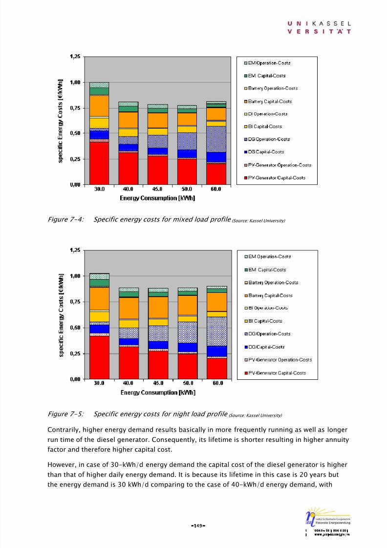
8/14/2019 Photovoltaic Systems Technology SS 2003
http://slidepdf.com/reader/full/photovoltaic-systems-technology-ss-2003 153/155
-149-t 0049- 561 804 6201i www.uni-kassel.de/re
Figure 7-4: Specific energy costs for mixed load profile (Source: Kassel University)
Figure 7-5: Specific energy costs for night load profile (Source: Kassel University)
Contrarily, higher energy demand results basically in more frequently running as well as longer
run time of the diesel generator. Consequently, its lifetime is shorter resulting in higher annuity
factor and therefore higher capital cost.
However, in case of 30-kWh/d energy demand the capital cost of the diesel generator is higher
than that of higher daily energy demand. It is because its lifetime in this case is 20 years but
the energy demand is 30 kWh/d comparing to the case of 40-kWh/d energy demand, with
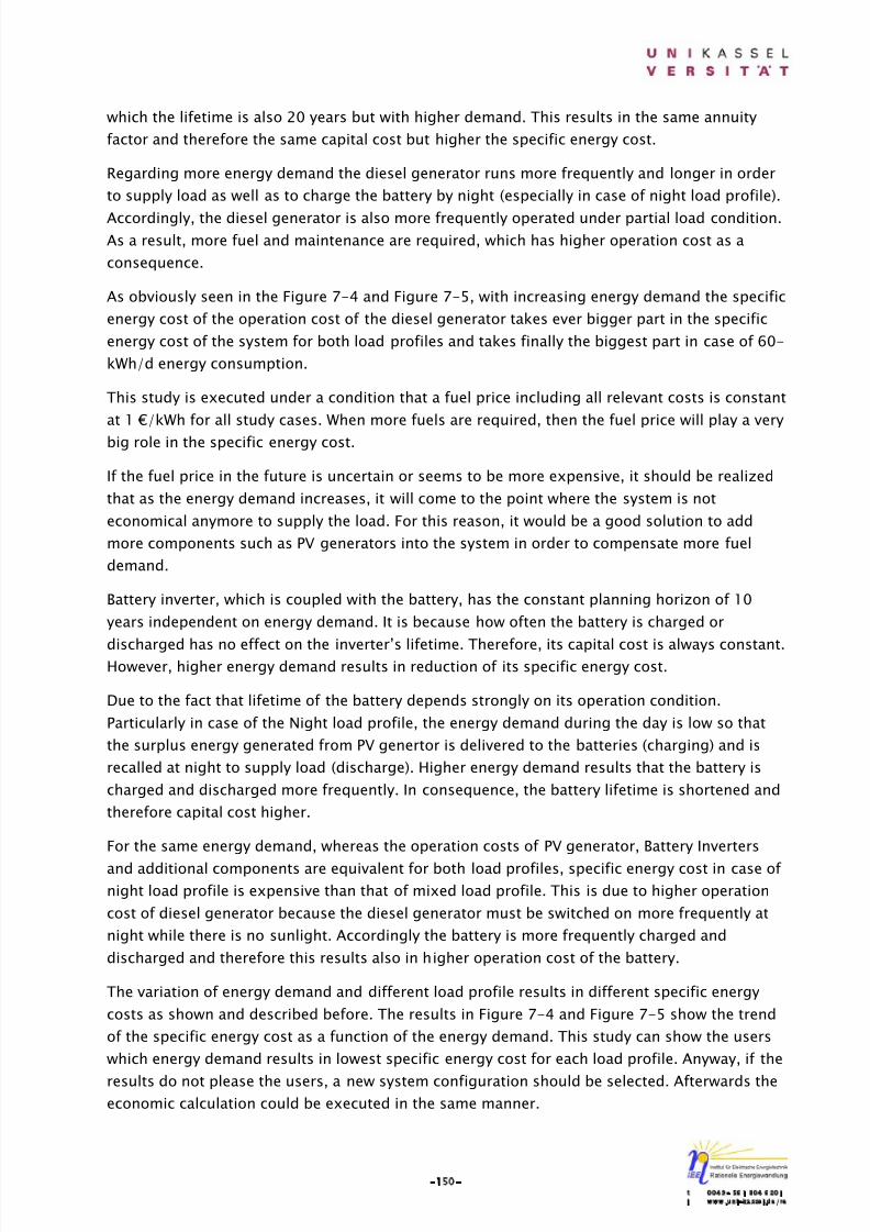
8/14/2019 Photovoltaic Systems Technology SS 2003
http://slidepdf.com/reader/full/photovoltaic-systems-technology-ss-2003 154/155
-150-t 0049- 561 804 6201i www.uni-kassel.de/re
which the lifetime is also 20 years but with higher demand. This results in the same annuity
factor and therefore the same capital cost but higher the specific energy cost.
Regarding more energy demand the diesel generator runs more frequently and longer in order
to supply load as well as to charge the battery by night (especially in case of night load profile).
Accordingly, the diesel generator is also more frequently operated under partial load condition.As a result, more fuel and maintenance are required, which has higher operation cost as a
consequence.
As obviously seen in the Figure 7-4 and Figure 7-5, with increasing energy demand the specific
energy cost of the operation cost of the diesel generator takes ever bigger part in the specific
energy cost of the system for both load profiles and takes finally the biggest part in case of 60-
kWh/d energy consumption.
This study is executed under a condition that a fuel price including all relevant costs is constant
at 1 €/kWh for all study cases. When more fuels are required, then the fuel price will play a very
big role in the specific energy cost.
If the fuel price in the future is uncertain or seems to be more expensive, it should be realized
that as the energy demand increases, it will come to the point where the system is not
economical anymore to supply the load. For this reason, it would be a good solution to add
more components such as PV generators into the system in order to compensate more fuel
demand.
Battery inverter, which is coupled with the battery, has the constant planning horizon of 10
years independent on energy demand. It is because how often the battery is charged or
discharged has no effect on the inverter’s lifetime. Therefore, its capital cost is always constant.However, higher energy demand results in reduction of its specific energy cost.
Due to the fact that lifetime of the battery depends strongly on its operation condition.
Particularly in case of the Night load profile, the energy demand during the day is low so that
the surplus energy generated from PV genertor is delivered to the batteries (charging) and is
recalled at night to supply load (discharge). Higher energy demand results that the battery is
charged and discharged more frequently. In consequence, the battery lifetime is shortened and
therefore capital cost higher.
For the same energy demand, whereas the operation costs of PV generator, Battery Inverters
and additional components are equivalent for both load profiles, specific energy cost in case of night load profile is expensive than that of mixed load profile. This is due to higher operation
cost of diesel generator because the diesel generator must be switched on more frequently at
night while there is no sunlight. Accordingly the battery is more frequently charged and
discharged and therefore this results also in higher operation cost of the battery.
The variation of energy demand and different load profile results in different specific energy
costs as shown and described before. The results in Figure 7-4 and Figure 7-5 show the trend
of the specific energy cost as a function of the energy demand. This study can show the users
which energy demand results in lowest specific energy cost for each load profile. Anyway, if the
results do not please the users, a new system configuration should be selected. Afterwards theeconomic calculation could be executed in the same manner.

8/14/2019 Photovoltaic Systems Technology SS 2003
http://slidepdf.com/reader/full/photovoltaic-systems-technology-ss-2003 155/155
7.5 References
[1] Finck, H.; Oelert, G.: A guide to the financial evaluation of investment projects in
energy supply . Deutsche Gesellschaft für Technische Zusammenarbeit (GTZ) GmbH,
Eschborn, ISBN 3-88085-250-2.