phased array ultrasonic examination of reactor coolant
TRANSCRIPT
PNNL-24920
Phased Array Ultrasonic Examination of Reactor Coolant System (Carbon Steel-to-CASS) Dissimilar Metal Weld Mockup Specimen
November 2015
SL Crawford AA Diaz AD Cinson MT Anderson
PNNL-24920
Phased Array Ultrasonic Examination of Reactor Coolant System (Carbon Steel-to-CASS) Dissimilar Metal Weld Mockup Specimen SL Crawford AA Diaz AD Cinson1 MT Anderson November 2015 Prepared for the U.S. Nuclear Regulatory Commission under a Related Services Agreement with the U.S. Department of Energy Contract DE-AC05-76RL01830 Pacific Northwest National Laboratory Richland, Washington 99352
1 U.S. Nuclear Regulatory Commission Washington, D.C. 20555

iii
Abstract
In the summer of 2009, Pacific Northwest National Laboratory (PNNL) staff traveled to the Electric Power Research Institute (EPRI) NDE Center in Charlotte, North Carolina, to conduct phased array ultrasonic testing on a large-bore, reactor coolant system pipe/elbow-to-safe-end mockup. This mockup was fabricated by FlawTech, Inc. and the configuration originated from the Port St. Lucie nuclear power plant. These plants are Combustion Engineering-designed reactors. This mockup consists of a carbon steel elbow with stainless steel cladding joined to a cast austenitic stainless steel (CASS) safe-end with a dissimilar metal weld and is owned by Florida Power & Light.
The objective of this study, and the data acquisition exercise held at the EPRI NDE Center, were focused on evaluating the capabilities of advanced, low-frequency phased array ultrasonic testing (PA-UT) examination techniques for detection and characterization of implanted circumferential flaws and machined reflectors in a thick-section CASS dissimilar metal weld component. This work was limited to PA-UT assessments using 500 kHz and 800 kHz probes on circumferential flaws only, and evaluated detection and characterization of these flaws and machined reflectors from the CASS safe-end side only. All data were obtained using spatially encoded, manual scanning techniques. The effects of such factors as line-scan versus raster-scan examination approaches were evaluated, and PA-UT detection and characterization performance as a function of inspection frequency/wavelength, were also assessed.
A comparative assessment of the data is provided, using length-sizing root-mean-square-error and position/localization results (flaw start/stop information) as the key criteria for flaw characterization performance. In addition, flaw signal-to-noise ratio was identified as the key criteria for detection performance.

v
Summary
This Technical Letter Report (TLR) summarizes a limited study conducted to assess the capabilities of phased array ultrasonic testing (PA-UT) as applied to a large bore, reactor coolant system elbow-to-safe-end mockup consisting of a carbon steel nozzle joined to a cast austenitic stainless steel (CASS) safe-end with a dissimilar metal weld (DMW). This work, which represents a sub-set of a multi-faceted program on the examination of CASS materials and welds, contributes to the understanding of the challenges and benefits involved in the inspections of these large-bore component configurations when using low-frequency, manual, spatially encoded PA-UT examinations. The results of PNNL’s research on inspection of CASS components can be used by the NRC staff to provide a basis for rulemaking and to assess new proposals such as those put forth by industry in ASME Code, Section XI, Appendix VIII, Supplement 9 for performance demonstration requirements for UT of CASS.
The mockup was designed from specifications based on existing reactor coolant system pipe/elbow-to-safe-end configurations in the Port St. Lucie nuclear plant. This reactor is of a Combustion Engineering-plant design. The mockup contained a total of 14 flaws, including both implanted thermal fatigue cracks (TFCs) and electro-discharge machined (EDM) notches in both circumferential and axial orientations. The flaws were located both in and near the welded region, including the butter. Additionally, some flaws were placed in the CASS safe-end material. While the mockup contained both axially and circumferentially oriented flaws, only the circumferentially oriented flaws were examined. This subset of the 14 implanted flaws included 6 TFCs and 3 EDM notches. During this evaluation PA-UT data were acquired only from the CASS (safe-end) side of the weld, which is considered to be the material most challenging to UT examination.
All six TFCs were detected by line and raster scans using 500 and 800 kHz probes. The three EDM notches were placed in the CASS pipe material away from the weld/butter region in close proximity to an inner diameter (ID) counterbore. A strong response from the counterbore at times masked the notch response, but the three EDM notches were detected with either line or raster scans at 500 or 800 kHz. The approximately 80 percent through-wall deep notch was detected with all four inspection techniques.
Length-sizing accuracy was assessed with root-mean-square-error (RMSE) calculations for all nine reflectors for each frequency and scanning method. Sizing at a −6 dB level as measured at the specimen outer diameter (i.e., not corrected for specimen curvature) gave the least error. Depending on probe frequency and scanning method, the RMSE values were between 9.5 and 12.7 mm (0.37 and 0.50 in.) and within the American Society of Mechanical Engineers (ASME) Boiler and Pressure Vessel Code, Section XI, length-sizing acceptance criterion of RMSE value less than 19.05 mm (0.75 in).
Depth sizing was performed only when flaw tip-diffracted signals were observed. Flaw tip signals were generally not observed for the shallow flaws (< 15 mm or 0.59 in.) as they were masked by the ID corner signal. Depth-sizing error values as measured by RMSE, 5.4 mm (0.21 in.) for 500 kHz data and 7.9 mm (0.31 in.) for 800 kHz data, were above the ASME Code criterion of less than 3.81 mm (0.125 in.). Flaw tilt and geometrical limitations on axial access to two deeper flaws perhaps led to higher error values. If these data points were removed, the RMSE values for raster data were within the ASME criterion. Other, non-standard depth-sizing methods such as loss-of-signal, full matrix capture, and/or non-linear acoustic post-processing techniques could be explored to assess their potential for providing through-wall depth information of flaws when detected in CASS; however, these activities were beyond the scope of the work reported here.
vi
Average signal-to-noise ratio (SNR) values for the 500 kHz data were nominally 16 dB (≈6:1) for line-scan data and 14 dB (≈5:1) for raster data. The SNR values in the 800 kHz data were approximately 12.7 dB (≈4:1), for both line and raster data. While the 800 kHz data provide better flaw resolution, there is typically an increase in grain noise leading to the lower SNR value as compared to the 500 kHz data. This was anticipated, and is predominantly due to the fact that the wavelength is beginning to approach the average size of the CASS grain diameters, increasing the effects of attenuation (i.e., scatter) with increasing frequency.
Typically, raster-scan data are expected to provide better flaw characterization; however, the use of a manual scanner required coarser resolutions in the index axis and the sweep of refracted angles. This likely contributed to the mixed results in that raster data did not always enhance the flaw characterization when compared to line-scan data.
With regard to general mockup design and flaw placement relative to detection impact, it was observed that axial position, with respect to weld and counterbore geometry, of a circumferentially oriented flaw affected detection and depth sizing. Also, general conclusions resulting from this study indicate that acquisition of spatially encoded data is important to providing an effective means for both detection and characterization of flaws.
vii
Acknowledgments
The work reported here was sponsored by the U.S. Nuclear Regulatory Commission (NRC) under U.S. Department of Energy Contract DE-AC05-76RL01830; Pacific Northwest National Laboratory (PNNL) Project No. 62895; NRC JCN V6323. Mr. Wallace Norris was the NRC Program Monitor at the time this work was conducted. PNNL would like to thank Mr. Norris for his guidance and technical direction during this time. Ms. Carol Nove is the present Contracting Officer Representative for this Program, at the time of submission of this technical letter report, and the authors would like to thank her for reviewing the technical content. PNNL would like to thank Mr. Dan Nowakowski of Florida Power & Light (FP&L) for authorizing the use of this mockup for the work described here. PNNL would also like to thank the Electric Power Research Institute (EPRI) NDE Center, in Charlotte, North Carolina, for hosting PNNL and for providing access to the FP&L mockup specimen. In particular, PNNL is grateful to Mr. Doug Kull, James (Leif) Esp, and Ronald (Ronnie) Swain at the EPRI NDE Center for escorting the team while onsite at the facility, and for their hospitality and support during PNNL’s data acquisition activities.
At PNNL, the authors wish to thank Ms. Katie Holton for her coordination and support of PNNL project logistics and for her help in handling travel-related reporting. PNNL is indebted to Mr. Royce Mathews, for providing in-laboratory support in packing and shipping the necessary equipment for the data acquisition effort. The team would also like to extend their gratitude to Ms. Lori Bisping for all of her hard work in providing administrative and financial reporting support to this project. Finally, the authors would like to extend their thanks to Ms. Kay Hass for her ongoing support, attention to detail, and technical editing expertise in preparing and finalizing this technical letter report.
PNNL is operated by Battelle for the U.S. Department of Energy under Contract DE-AC05-76RL01830.

ix
Acronyms and Abbreviations
ASME American Society of Mechanical Engineers CASS cast austenitic stainless steel dB decibels DMW dissimilar metal weld EDM electro-discharge machined EPRI Electric Power Research Institute FP&L Florida Power & Light ID inner diameter ISI inservice inspection kHz kilohertz LOS loss-of-signal MHz megahertz NDE nondestructive examination or evaluation NRC U.S. Nuclear Regulatory Commission OD outside diameter PA phased array PA-UT phased array ultrasonic testing PNNL Pacific Northwest National Laboratory RMSE root mean square error SAFT Synthetic Aperture Focusing Technique SNR signal-to-noise TFC thermal fatigue crack TRL transmit-receive longitudinal UT ultrasonic testing

xi
Contents
Abstract ........................................................................................................................................................ iii Summary ....................................................................................................................................................... v Acknowledgments ....................................................................................................................................... vii Acronyms and Abbreviations ...................................................................................................................... ix 1.0 Introduction ....................................................................................................................................... 1.1 2.0 Objective and Scope .......................................................................................................................... 2.1 3.0 Florida Power & Light Mockup Specimen ........................................................................................ 3.1 4.0 Phased-Array Probes and Simulated Sound Fields ........................................................................... 4.1 5.0 Basis for Using Longer Wavelengths (Lower Frequencies) .............................................................. 5.1 6.0 PA-UT Mockup Data Acquisition ..................................................................................................... 6.1 7.0 Data Analyses and Summary of PA-UT Results ............................................................................... 7.1
7.1 500 kHz Results ........................................................................................................................ 7.1 7.2 800 kHz PA-UT Data Results ................................................................................................... 7.9
8.0 Discussion and Conclusions .............................................................................................................. 8.1 8.1 Discussion ................................................................................................................................. 8.1 8.2 Conclusions ............................................................................................................................... 8.2
9.0 References ......................................................................................................................................... 9.1 Appendix A – 500 kHz and 800 kHz PA-UT Line-Scan and Raster-Scan Data Images .......................... A.1 Appendix B – Merged Line-Scan Data over Entire Specimen Circumference ..........................................B.1
xii
Figures
3.1 Port St. Lucie FP&L Reactor Coolant System DMW Mockup at the EPRI NDE Center ................. 3.1 3.2 Design Drawing Showing the Overall Nominal Dimensions of the FP&L Mockup with
Material Types ................................................................................................................................... 3.2 3.3 Design Drawing Illustrating the Weld Prep Geometry and Nominal Dimensions and Angles
for the DMW ...................................................................................................................................... 3.3 3.4 Design Drawing Illustrating the Flaw-Section View, Pipe-End View, and Flaw
Specifications for Flaws Numbered 1 through 4 ............................................................................... 3.3 3.5 Design Drawing Illustrating the Flaw-Section View, Pipe-End View, and Flaw
Specifications for Flaws Numbered 5 through 8 ............................................................................... 3.4 3.6 Design Drawing Illustrating the Flaw-Section View, Pipe-End View, and Flaw
Specifications for Flaws Numbered 9 through 12 ............................................................................. 3.4 3.7 Design Drawing Illustrating the Flaw-Section View, Pipe-End View, and Flaw
Specifications for Flaws Numbered 13 and 14 .................................................................................. 3.5 4.1 Phased Array Probes with Center Frequencies of 500 kHz and 800 kHz .......................................... 4.1 4.2 Simulated −3 dB Sound Beam B-scan Views and C-scan Views of the Focal Spot for the
500 kHz and 800 kHz PA-UT Probes Used in This Study ................................................................ 4.2 6.1 Data Acquisition System and Laboratory Workstation ..................................................................... 6.1 7.1 Line-Scan Data for TFC #1 at 500 kHz ............................................................................................. 7.1 7.2 Raster Scan Data for TFC #1 ............................................................................................................. 7.2 7.3 EDM Flaw #11 Line Scan Data; Flaw is Not Detected ..................................................................... 7.5 7.4 EDM Flaw #12 Line Scan Data; Flaw is Detected ............................................................................ 7.6 7.5 Flaw Tip Response Indicated by the Red Arrows in 500 kHz Line-Scan Data for TFC #8 .............. 7.7 7.6 Flaw Tip Response Indicated by the Red Arrows in 500 kHz Raster Scan Data for TFC #8 ........... 7.7 7.7 Flaw #1 Raster-Scan Response with 500 kHz Data on the Left and 800 kHz Data on the
Right ................................................................................................................................................ 7.12 7.8 Flaw #5 Raster Scan Response with 500 kHz Data on the Left and 800 kHz Data on the
Right ................................................................................................................................................ 7.12
xiii
Tables
3.1 True-State Flaw Distribution and Specification List ......................................................................... 3.2 4.1 Probe Size Information ...................................................................................................................... 4.1 5.1 Approximate Acoustic Wavelengths in the Mockup ......................................................................... 5.2 7.1 Length Sizing for 500 kHz Data (mm) .............................................................................................. 7.3 7.2 Length Sizing for 500 kHz Data (in.) ................................................................................................ 7.4 7.3 Depth Sizing for 500 kHz Data .......................................................................................................... 7.8 7.4 SNR for 500 kHz Data ....................................................................................................................... 7.9 7.5 Length Sizing for 800 kHz Data (mm) ............................................................................................ 7.10 7.6 Length Sizing for 800 kHz Data (in.) .............................................................................................. 7.10 7.7 Depth Sizing for 800 kHz Data ........................................................................................................ 7.11 7.8 SNR for 800 kHz Data ..................................................................................................................... 7.11

1.1
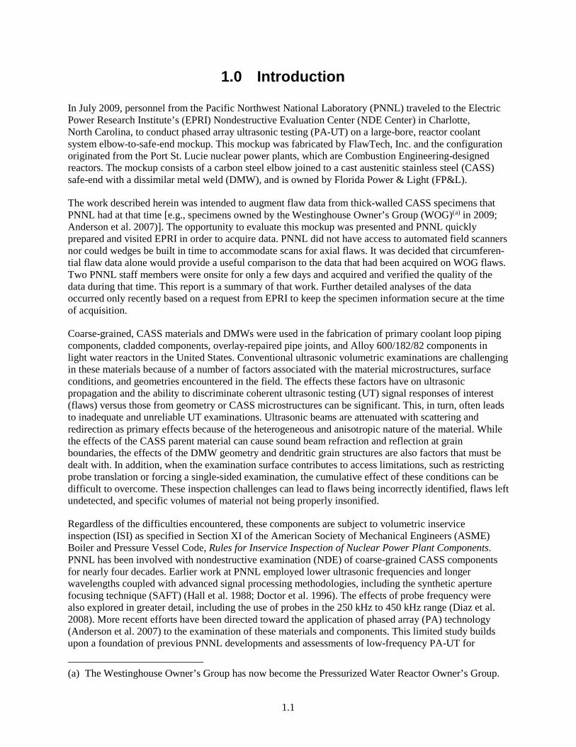
1.0 Introduction
In July 2009, personnel from the Pacific Northwest National Laboratory (PNNL) traveled to the Electric Power Research Institute’s (EPRI) Nondestructive Evaluation Center (NDE Center) in Charlotte, North Carolina, to conduct phased array ultrasonic testing (PA-UT) on a large-bore, reactor coolant system elbow-to-safe-end mockup. This mockup was fabricated by FlawTech, Inc. and the configuration originated from the Port St. Lucie nuclear power plants, which are Combustion Engineering-designed reactors. The mockup consists of a carbon steel elbow joined to a cast austenitic stainless steel (CASS) safe-end with a dissimilar metal weld (DMW), and is owned by Florida Power & Light (FP&L).
The work described herein was intended to augment flaw data from thick-walled CASS specimens that PNNL had at that time [e.g., specimens owned by the Westinghouse Owner’s Group (WOG)(a) in 2009; Anderson et al. 2007)]. The opportunity to evaluate this mockup was presented and PNNL quickly prepared and visited EPRI in order to acquire data. PNNL did not have access to automated field scanners nor could wedges be built in time to accommodate scans for axial flaws. It was decided that circumferen-tial flaw data alone would provide a useful comparison to the data that had been acquired on WOG flaws. Two PNNL staff members were onsite for only a few days and acquired and verified the quality of the data during that time. This report is a summary of that work. Further detailed analyses of the data occurred only recently based on a request from EPRI to keep the specimen information secure at the time of acquisition.
Coarse-grained, CASS materials and DMWs were used in the fabrication of primary coolant loop piping components, cladded components, overlay-repaired pipe joints, and Alloy 600/182/82 components in light water reactors in the United States. Conventional ultrasonic volumetric examinations are challenging in these materials because of a number of factors associated with the material microstructures, surface conditions, and geometries encountered in the field. The effects these factors have on ultrasonic propagation and the ability to discriminate coherent ultrasonic testing (UT) signal responses of interest (flaws) versus those from geometry or CASS microstructures can be significant. This, in turn, often leads to inadequate and unreliable UT examinations. Ultrasonic beams are attenuated with scattering and redirection as primary effects because of the heterogeneous and anisotropic nature of the material. While the effects of the CASS parent material can cause sound beam refraction and reflection at grain boundaries, the effects of the DMW geometry and dendritic grain structures are also factors that must be dealt with. In addition, when the examination surface contributes to access limitations, such as restricting probe translation or forcing a single-sided examination, the cumulative effect of these conditions can be difficult to overcome. These inspection challenges can lead to flaws being incorrectly identified, flaws left undetected, and specific volumes of material not being properly insonified.
Regardless of the difficulties encountered, these components are subject to volumetric inservice inspection (ISI) as specified in Section XI of the American Society of Mechanical Engineers (ASME) Boiler and Pressure Vessel Code, Rules for Inservice Inspection of Nuclear Power Plant Components. PNNL has been involved with nondestructive examination (NDE) of coarse-grained CASS components for nearly four decades. Earlier work at PNNL employed lower ultrasonic frequencies and longer wavelengths coupled with advanced signal processing methodologies, including the synthetic aperture focusing technique (SAFT) (Hall et al. 1988; Doctor et al. 1996). The effects of probe frequency were also explored in greater detail, including the use of probes in the 250 kHz to 450 kHz range (Diaz et al. 2008). More recent efforts have been directed toward the application of phased array (PA) technology (Anderson et al. 2007) to the examination of these materials and components. This limited study builds upon a foundation of previous PNNL developments and assessments of low-frequency PA-UT for
(a) The Westinghouse Owner’s Group has now become the Pressurized Water Reactor Owner’s Group.
1.2
evaluating improved detection and characterization of flaws in DMWs and CASS components. The examinations were conducted using two different PA probes operating at nominal center frequencies of 500 and 800 kHz, and represent probes specifically designed for the evaluation of thick-section, coarse-grained materials.
There has currently been no operational experience with service-induced degradation in CASS piping. Further, it is unclear as to the type(s) of service degradation that may be expected in these materials. However, ASME Section XI requires the examination of welded areas, as these present a material and structural discontinuity in piping systems. The DMW examined as the subject of this report was fabricated with implanted thermal fatigue cracks (TFCs) placed in the weld material, along with machined notches. It is probable that the owner of the specimen intended the implanted flaws to simulate UT responses from primary water stress corrosion cracks, as this is an active degradation mechanism in DMWs. It is unclear whether FP&L planned on using the notches as simulated flaws or calibration reflectors, but these may be used for either purpose. In any event, the FP&L specimen afforded PNNL the opportunity to examine simulated cracks by insonifying from the CASS side of the weld; thus, it was appropriate for that purpose.
This technical letter report (TLR) provides a summary of the study that was conducted at both the EPRI NDE Center (in July of 2009) and the subsequent data analysis at PNNL. The TLR is organized with Section 2.0 providing the objectives and scope of the work. Section 3.0 describes the design of the FP&L mockup, the materials used, and the flaws introduced into the specimen by FlawTech, Inc. PA-UT probe specifications and modeling results (beam simulations) are provided in Section 4.0, while the basis for employing lower frequencies and longer wavelengths is described in Section 5.0. The experimental setup and data acquisition protocol are documented in Section 6.0. Ultrasonic data and analyses are presented in Section 7.0. Lastly, a discussion and conclusions are presented in Section 8.0 with references listed in Section 9.0. Supporting documentation, including line- and raster-scan images from the 500 kHz and 800 kHz examinations, are provided in Appendices A and B.
2.1
2.0 Objective and Scope
The objective of this study, and the data acquisition exercise held at the EPRI NDE Center in 2009, was to evaluate the capabilities of advanced, low-frequency PA-UT examination techniques for detection and characterization of circumferential flaws in thick-section CASS DMW components. In particular, the scope of the work included access to a reactor coolant system mockup, owned by FP&L that resided at the EPRI NDE Center at that time. This mockup (fabricated from the Combustion Engineering-plant design for a Port St. Lucie elbow-to-safe end configuration) was fabricated by FlawTech and contained sets of TFCs and electro-discharge machined (EDM) notches in both axial and circumferential orientations. The scope of this work was limited to an assessment of circumferentially oriented flaws only, and evaluated detection and characterization of flaws from the CASS safe-end side only, which is the material most challenging to UT propagation. The effects of such factors as line-scan versus raster-scan examination approaches were studied, and the detection and characterization performance as a function of UT frequency, and thus wavelength, were also evaluated. It should be noted that the data acquisition exercise reported herein was performed in an open fashion; that is, PNNL staff were aware of the location of the flaws in the mockup.
For this study, 500 kHz and 800 kHz probes were employed for simulations and data acquisition activities. All data were obtained using spatially encoded, manual scanning techniques. In order to better understand the cumulative effects of the CASS material and DMW geometry on the examination effectiveness, the effects of the input ultrasonic inspection parameters such as probe center frequency and refracted and skew angles were evaluated and discussed with respect to the true-state flaw locations and dimensions. A comparative assessment was conducted (with respect to design drawings and true-state data) using length-sizing root-mean-square-error (RMSE) and position/localization data (flaw start/stop information) as the key criteria for flaw characterization performance. In addition, minimum flaw signal-to-noise ratio (SNR) values were identified as a key criterion for detection performance.

3.1
3.0 Florida Power & Light Mockup Specimen
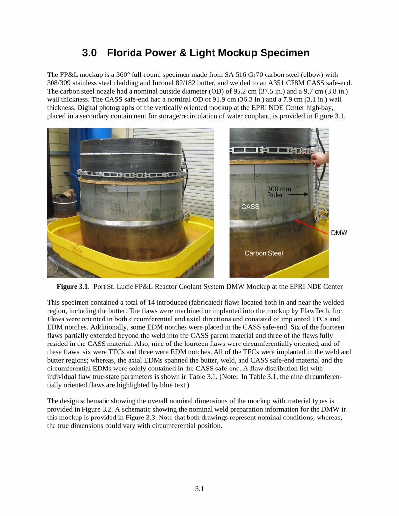
The FP&L mockup is a 360° full-round specimen made from SA 516 Gr70 carbon steel (elbow) with 308/309 stainless steel cladding and Inconel 82/182 butter, and welded to an A351 CF8M CASS safe-end. The carbon steel nozzle had a nominal outside diameter (OD) of 95.2 cm (37.5 in.) and a 9.7 cm (3.8 in.) wall thickness. The CASS safe-end had a nominal OD of 91.9 cm (36.3 in.) and a 7.9 cm (3.1 in.) wall thickness. Digital photographs of the vertically oriented mockup at the EPRI NDE Center high-bay, placed in a secondary containment for storage/recirculation of water couplant, is provided in Figure 3.1.
Figure 3.1. Port St. Lucie FP&L Reactor Coolant System DMW Mockup at the EPRI NDE Center
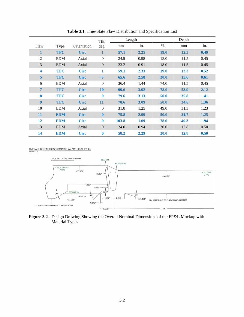
This specimen contained a total of 14 introduced (fabricated) flaws located both in and near the welded region, including the butter. The flaws were machined or implanted into the mockup by FlawTech, Inc. Flaws were oriented in both circumferential and axial directions and consisted of implanted TFCs and EDM notches. Additionally, some EDM notches were placed in the CASS safe-end. Six of the fourteen flaws partially extended beyond the weld into the CASS parent material and three of the flaws fully resided in the CASS material. Also, nine of the fourteen flaws were circumferentially oriented, and of these flaws, six were TFCs and three were EDM notches. All of the TFCs were implanted in the weld and butter regions; whereas, the axial EDMs spanned the butter, weld, and CASS safe-end material and the circumferential EDMs were solely contained in the CASS safe-end. A flaw distribution list with individual flaw true-state parameters is shown in Table 3.1. (Note: In Table 3.1, the nine circumferen-tially oriented flaws are highlighted by blue text.)
The design schematic showing the overall nominal dimensions of the mockup with material types is provided in Figure 3.2. A schematic showing the nominal weld preparation information for the DMW in this mockup is provided in Figure 3.3. Note that both drawings represent nominal conditions; whereas, the true dimensions could vary with circumferential position.
3.2
Table 3.1. True-State Flaw Distribution and Specification List
Flaw Type Orientation Tilt, deg.
Length Depth mm in. % mm in.
1 TFC Circ 1 57.1 2.25 19.0 12.5 0.49 2 EDM Axial 0 24.9 0.98 18.0 11.5 0.45 3 EDM Axial 0 23.2 0.91 18.0 11.5 0.45 4 TFC Circ 1 59.1 2.33 19.0 13.3 0.52 5 TFC Circ −3 65.6 2.58 20.0 15.6 0.61 6 EDM Axial 0 36.4 1.44 74.0 11.5 0.45 7 TFC Circ 10 99.6 3.92 78.0 53.9 2.12 8 TFC Circ 0 79.6 3.13 50.0 35.8 1.41 9 TFC Circ 11 78.6 3.09 50.0 34.6 1.36
10 EDM Axial 0 31.8 1.25 49.0 31.3 1.23 11 EDM Circ 0 75.8 2.99 50.0 31.7 1.25 12 EDM Circ 0 103.8 1.09 78.0 49.3 1.94 13 EDM Axial 0 24.0 0.94 20.0 12.8 0.50 14 EDM Circ 0 58.2 2.29 20.0 12.8 0.50
Figure 3.2. Design Drawing Showing the Overall Nominal Dimensions of the FP&L Mockup with
Material Types
3.3
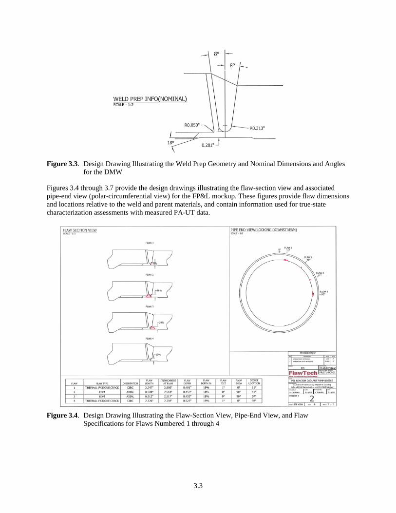
Figure 3.3. Design Drawing Illustrating the Weld Prep Geometry and Nominal Dimensions and Angles
for the DMW
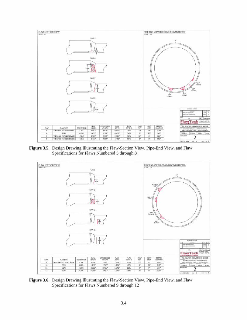
Figures 3.4 through 3.7 provide the design drawings illustrating the flaw-section view and associated pipe-end view (polar-circumferential view) for the FP&L mockup. These figures provide flaw dimensions and locations relative to the weld and parent materials, and contain information used for true-state characterization assessments with measured PA-UT data.
Figure 3.4. Design Drawing Illustrating the Flaw-Section View, Pipe-End View, and Flaw
Specifications for Flaws Numbered 1 through 4
3.4
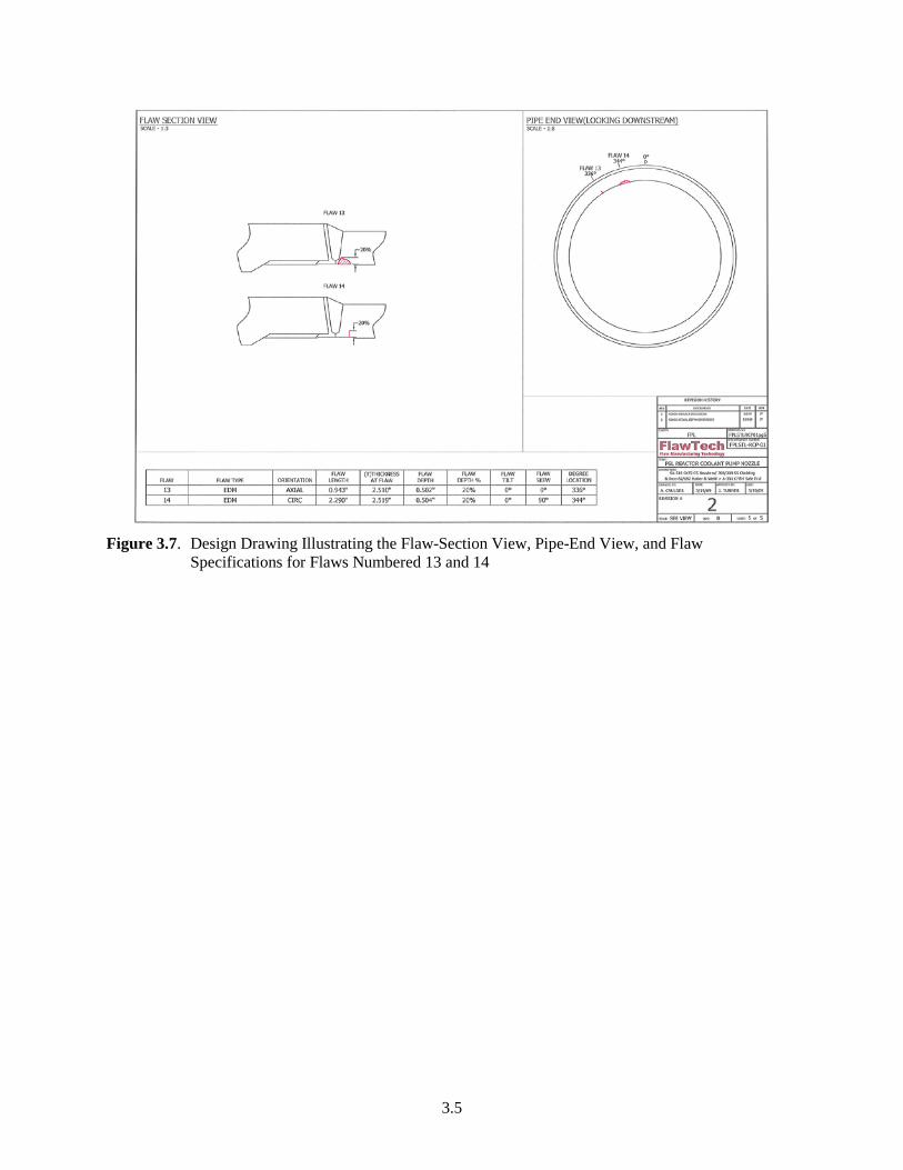
Figure 3.5. Design Drawing Illustrating the Flaw-Section View, Pipe-End View, and Flaw
Specifications for Flaws Numbered 5 through 8
Figure 3.6. Design Drawing Illustrating the Flaw-Section View, Pipe-End View, and Flaw
Specifications for Flaws Numbered 9 through 12
3.5
Figure 3.7. Design Drawing Illustrating the Flaw-Section View, Pipe-End View, and Flaw
Specifications for Flaws Numbered 13 and 14

4.1
4.0 Phased Array Probes and Simulated Sound Fields
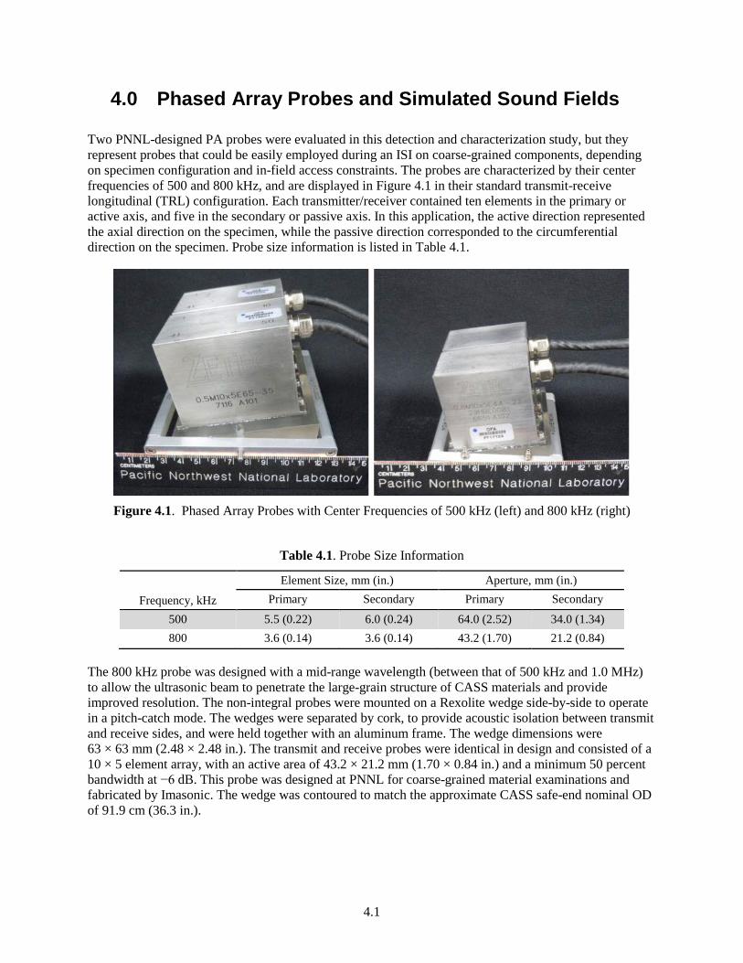
Two PNNL-designed PA probes were evaluated in this detection and characterization study, but they represent probes that could be easily employed during an ISI on coarse-grained components, depending on specimen configuration and in-field access constraints. The probes are characterized by their center frequencies of 500 and 800 kHz, and are displayed in Figure 4.1 in their standard transmit-receive longitudinal (TRL) configuration. Each transmitter/receiver contained ten elements in the primary or active axis, and five in the secondary or passive axis. In this application, the active direction represented the axial direction on the specimen, while the passive direction corresponded to the circumferential direction on the specimen. Probe size information is listed in Table 4.1.
Figure 4.1. Phased Array Probes with Center Frequencies of 500 kHz (left) and 800 kHz (right)
Table 4.1. Probe Size Information
Frequency, kHz
Element Size, mm (in.) Aperture, mm (in.) Primary Secondary Primary Secondary
500 5.5 (0.22) 6.0 (0.24) 64.0 (2.52) 34.0 (1.34) 800 3.6 (0.14) 3.6 (0.14) 43.2 (1.70) 21.2 (0.84)
The 800 kHz probe was designed with a mid-range wavelength (between that of 500 kHz and 1.0 MHz) to allow the ultrasonic beam to penetrate the large-grain structure of CASS materials and provide improved resolution. The non-integral probes were mounted on a Rexolite wedge side-by-side to operate in a pitch-catch mode. The wedges were separated by cork, to provide acoustic isolation between transmit and receive sides, and were held together with an aluminum frame. The wedge dimensions were 63 × 63 mm (2.48 × 2.48 in.). The transmit and receive probes were identical in design and consisted of a 10 × 5 element array, with an active area of 43.2 × 21.2 mm (1.70 × 0.84 in.) and a minimum 50 percent bandwidth at −6 dB. This probe was designed at PNNL for coarse-grained material examinations and fabricated by Imasonic. The wedge was contoured to match the approximate CASS safe-end nominal OD of 91.9 cm (36.3 in.).
4.2
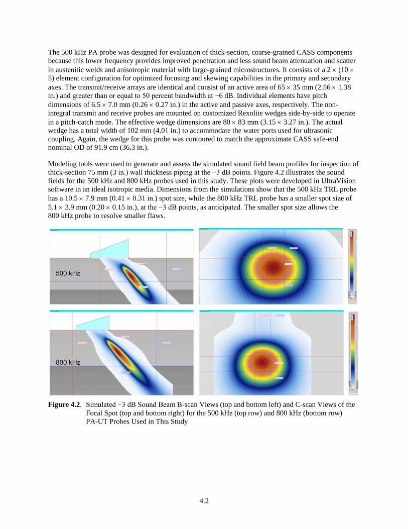
The 500 kHz PA probe was designed for evaluation of thick-section, coarse-grained CASS components because this lower frequency provides improved penetration and less sound beam attenuation and scatter in austenitic welds and anisotropic material with large-grained microstructures. It consists of a 2 × (10 × 5) element configuration for optimized focusing and skewing capabilities in the primary and secondary axes. The transmit/receive arrays are identical and consist of an active area of 65 × 35 mm (2.56 × 1.38 in.) and greater than or equal to 50 percent bandwidth at −6 dB. Individual elements have pitch dimensions of 6.5 × 7.0 mm (0.26 × 0.27 in.) in the active and passive axes, respectively. The non-integral transmit and receive probes are mounted on customized Rexolite wedges side-by-side to operate in a pitch-catch mode. The effective wedge dimensions are 80 × 83 mm (3.15 × 3.27 in.). The actual wedge has a total width of 102 mm (4.01 in.) to accommodate the water ports used for ultrasonic coupling. Again, the wedge for this probe was contoured to match the approximate CASS safe-end nominal OD of 91.9 cm (36.3 in.).
Modeling tools were used to generate and assess the simulated sound field beam profiles for inspection of thick-section 75 mm (3 in.) wall thickness piping at the −3 dB points. Figure 4.2 illustrates the sound fields for the 500 kHz and 800 kHz probes used in this study. These plots were developed in UltraVision software in an ideal isotropic media. Dimensions from the simulations show that the 500 kHz TRL probe has a 10.5 × 7.9 mm (0.41 × 0.31 in.) spot size, while the 800 kHz TRL probe has a smaller spot size of 5.1 × 3.9 mm (0.20 × 0.15 in.), at the −3 dB points, as anticipated. The smaller spot size allows the 800 kHz probe to resolve smaller flaws.
Figure 4.2. Simulated −3 dB Sound Beam B-scan Views (top and bottom left) and C-scan Views of the
Focal Spot (top and bottom right) for the 500 kHz (top row) and 800 kHz (bottom row) PA-UT Probes Used in This Study
5.1
5.0 Basis for Using Longer Wavelengths (Lower Frequencies)
CASS materials commonly used in nuclear power plants are polycrystalline coarse-grained materials that are elastically anisotropic. The interaction of ultrasonic waves with such material results in phenomena such as grain-to-grain sound speed variations, ultrasonic beam redirection and partitioning, large direction-dependent attenuation and background acoustic noise caused by grain-induced scattering, and phase variations across a wave front. These phenomena make reliable ultrasonic inspections highly challenging. Combining these material effects with scanning restrictions caused by access limitations and DMW geometries suggests the use of advanced ultrasonic methods that are capable of addressing these inspection challenges will improve detection and characterization performance over that of conventional UT techniques.
As acoustic waves interact with materials, scattering of energy occurs at interfaces such as grain boundaries. Scattering in the direction of a transmitting element is often referred to as backscatter. However, the scattered energy at any angle (relative to the transmit direction) can be measured, if a receiver can be placed appropriately. Scattering typically occurs if the mean scatterer (grain) size ( D ) is small or comparable to the wavelength (λ) of the acoustic wave, and a change in acoustic impedance is present across the grain boundary (Goebbels 1994). The contrast in acoustic impedance across a grain boundary can occur due to anisotropy of the elastic properties of grains and the different orientation of each grain (Thompson et al. 2008). In general, the scattering behavior of ultrasonic waves from single scatterers may be broadly classed into three regimes (Ensminger and Bond 2011)—Rayleigh, stochastic, and geometric. In the Rayleigh regime, the scatterer or grain size (d) is small relative to the wavelength of the acoustic wave used [typically, d/λ « 1 (Goebbels 1994)]. As the ratio of the grain size-to-wavelength increases, the interactions between the wave and the grains increases, resulting in increased amounts of scattering. In the large-grain limit (d/λ » 1), where the wavelength is much smaller than the grain size, the scattering behavior may be described using geometric principles. For intermediate wavelengths, however, the observed acoustic behavior is best described using stochastic methods. In CASS materials, the grain sizes can vary over a large range (Diaz et al. 2012) and, therefore, the scattering behavior can range from Rayleigh to geometric regimes in a single material volume. Thus, the mean grain size D is often used instead of the individual grain size d to describe the scatterer size and the dominant scattering regime.
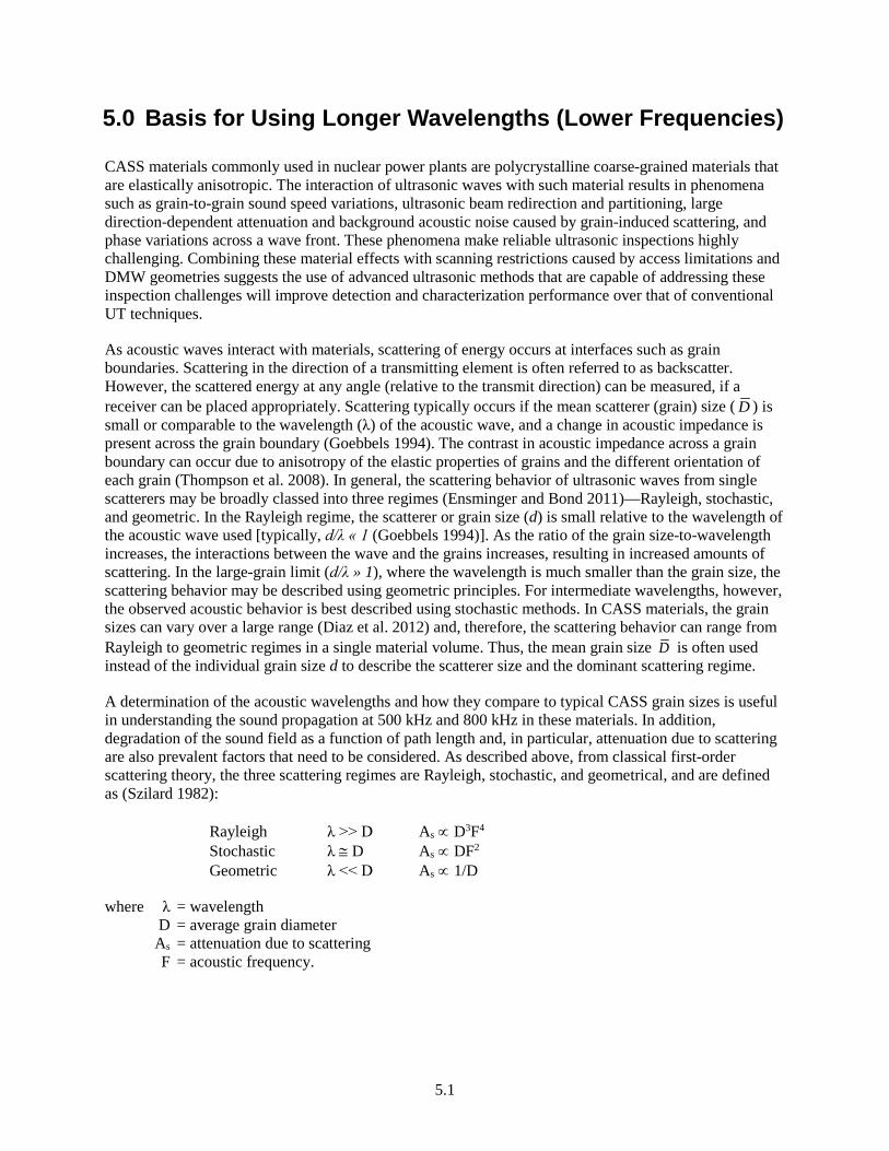
A determination of the acoustic wavelengths and how they compare to typical CASS grain sizes is useful in understanding the sound propagation at 500 kHz and 800 kHz in these materials. In addition, degradation of the sound field as a function of path length and, in particular, attenuation due to scattering are also prevalent factors that need to be considered. As described above, from classical first-order scattering theory, the three scattering regimes are Rayleigh, stochastic, and geometrical, and are defined as (Szilard 1982):
Rayleigh λ >> D As ∝ D3F4 Stochastic λ ≅ D As ∝ DF2 Geometric λ << D As ∝ 1/D
where λ = wavelength D = average grain diameter As = attenuation due to scattering F = acoustic frequency.
5.2
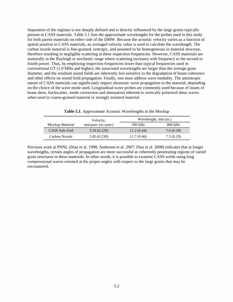
Separation of the regimes is not sharply defined and is directly influenced by the large grains typically present in CASS materials. Table 5.1 lists the approximate wavelengths for the probes used in this study for both parent materials on either side of the DMW. Because the acoustic velocity varies as a function of spatial position in CASS materials, an averaged velocity value is used to calculate the wavelength. The carbon nozzle material is fine-grained, isotropic, and assumed to be homogeneous in material structure, therefore resulting in negligible scattering at these inspection frequencies. However, CASS materials are nominally in the Rayleigh or stochastic range where scattering increases with frequency to the second or fourth power. Thus, by employing inspection frequencies lower than typical frequencies used in conventional UT (1.0 MHz and higher), the associated wavelengths are larger than the average grain diameter, and the resultant sound fields are inherently less sensitive to the degradation of beam coherence and other effects on sound field propagation. Finally, one must address wave modality. The anisotropic nature of CASS materials can significantly impact ultrasonic wave propagation in the material, depending on the choice of the wave mode used. Longitudinal-wave probes are commonly used because of issues of beam skew, backscatter, mode conversion and attenuation inherent to vertically polarized shear waves when used in coarse-grained material or strongly textured material.
Table 5.1. Approximate Acoustic Wavelengths in the Mockup
Mockup Material Velocity,
mm/µsec (in./µsec) Wavelength, mm (in.)
500 kHz 800 kHz CASS Safe-End 5.59 (0.220) 11.2 (0.44) 7.0 (0.28) Carbon Nozzle 5.85 (0.230) 11.7 (0.46) 7.3 (0.29)
Previous work at PNNL (Diaz et al. 1998; Anderson et al. 2007; Diaz et al. 2008) indicates that at longer wavelengths, certain angles of propagation are more successful at coherently penetrating regions of varied grain structures in these materials. In other words, it is possible to examine CASS welds using long compressional waves oriented at the proper angles with respect to the large grains that may be encountered.
6.1
6.0 PA-UT Mockup Data Acquisition
Set up and laboratory configuration for PA-UT data acquisition on the FP&L DMW mockup required the use of a ZETEC manual-encoded scanner mounted directly onto the pipe under inspection (preferred setup) as shown in Figure 3.1. The probe is mounted on an extension arm that is adjustable along the pipe axis. Two encoders on the manual track scanner provide 2D spatial information for both the axial and circumferential directions for line and raster scanning.
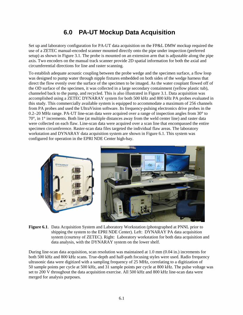
To establish adequate acoustic coupling between the probe wedge and the specimen surface, a flow loop was designed to pump water through nipple fixtures embedded on both sides of the wedge harness that direct the flow evenly over the surface of the specimen to be imaged. As the water couplant flowed off of the OD surface of the specimen, it was collected in a large secondary containment (yellow plastic tub), channeled back to the pump, and recycled. This is also illustrated in Figure 3.1. Data acquisition was accomplished using a ZETEC DYNARAY system for both 500 kHz and 800 kHz PA probes evaluated in this study. This commercially available system is equipped to accommodate a maximum of 256 channels from PA probes and used the UltraVision software. Its frequency-pulsing electronics drive probes in the 0.2–20 MHz range. PA-UT line-scan data were acquired over a range of inspection angles from 30° to 70°, in 1° increments. Both line (at multiple distances away from the weld center line) and raster data were collected on each flaw. Line-scan data were acquired over a scan line that encompassed the entire specimen circumference. Raster-scan data files targeted the individual flaw areas. The laboratory workstation and DYNARAY data acquisition system are shown in Figure 6.1. This system was configured for operation in the EPRI NDE Center high-bay.
Figure 6.1. Data Acquisition System and Laboratory Workstation (photographed at PNNL prior to
shipping the system to the EPRI NDE Center). Left: DYNARAY PA data acquisition system (courtesy of ZETEC). Right: Laboratory workstation for both data acquisition and data analysis, with the DYNARAY system on the lower shelf.
During line-scan data acquisition, scan resolution was maintained at 1.0 mm (0.04 in.) increments for both 500 kHz and 800 kHz scans. True-depth and half-path focusing styles were used. Radio frequency ultrasonic data were digitized with a sampling frequency of 25 MHz, correlating to a digitization of 50 sample points per cycle at 500 kHz, and 31 sample points per cycle at 800 kHz. The pulse voltage was set to 200 V throughout the data acquisition exercise. All 500 kHz and 800 kHz line-scan data were merged for analysis purposes.

6.2
During raster-scan data acquisition, scan resolution was changed. For both 500 kHz and 800 kHz raster scans, step-size resolution was maintained at 0.5 mm (0.02 in.) in the scan axis and 2.0 mm (0.08 in.) in the index axis. The focusing technique did not change; however, the angles obtained during raster scanning were modified to obtain data from 25° to 60° in 5° increments. Pulse voltage, digitization, and sampling were all kept identical to the line-scan protocol. UltraVision software version 3.2R6 was used for both data acquisition and analyses.
7.1
7.0 Data Analyses and Summary of PA-UT Results
The 500 and 800 kHz data were analyzed for flaw detection and flaw characterization as measured by flaw length, and depth sizing, as well as flaw SNR. Section 7.1 presents the 500 kHz data while Section 7.2 presents the 800 kHz data.
7.1 500 kHz Results
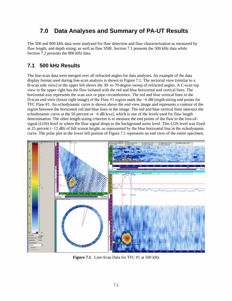
The line-scan data were merged over all refracted angles for data analyses. An example of the data display format used during line-scan analysis is shown in Figure 7.1. The sectorial view (similar to a B-scan side view) in the upper left shows the 30- to 70-degree sweep of refracted angles. A C-scan top view in the upper right has the flaw isolated with the red and blue horizontal and vertical lines. The horizontal axis represents the scan axis or pipe circumference. The red and blue vertical lines in the D-scan end view (lower right image) of the Flaw #1 region mark the −6 dB length-sizing end points for TFC Flaw #1. An echodynamic curve is shown above the end view image and represents a contour of the region between the horizontal red and blue lines in the image. The red and blue vertical lines intersect the echodynamic curve at the 50 percent or −6 dB level, which is one of the levels used for flaw length determination. The other length-sizing criterion is to measure the end points of the flaw to the loss-of-signal (LOS) level or where the flaw signal drops to the background noise level. This LOS level was fixed at 25 percent (−12 dB) of full screen height, as represented by the blue horizontal line in the echodynamic curve. The polar plot in the lower left portion of Figure 7.1 represents an end view of the entire specimen.
Figure 7.1. Line-Scan Data for TFC #1 at 500 kHz
7.2
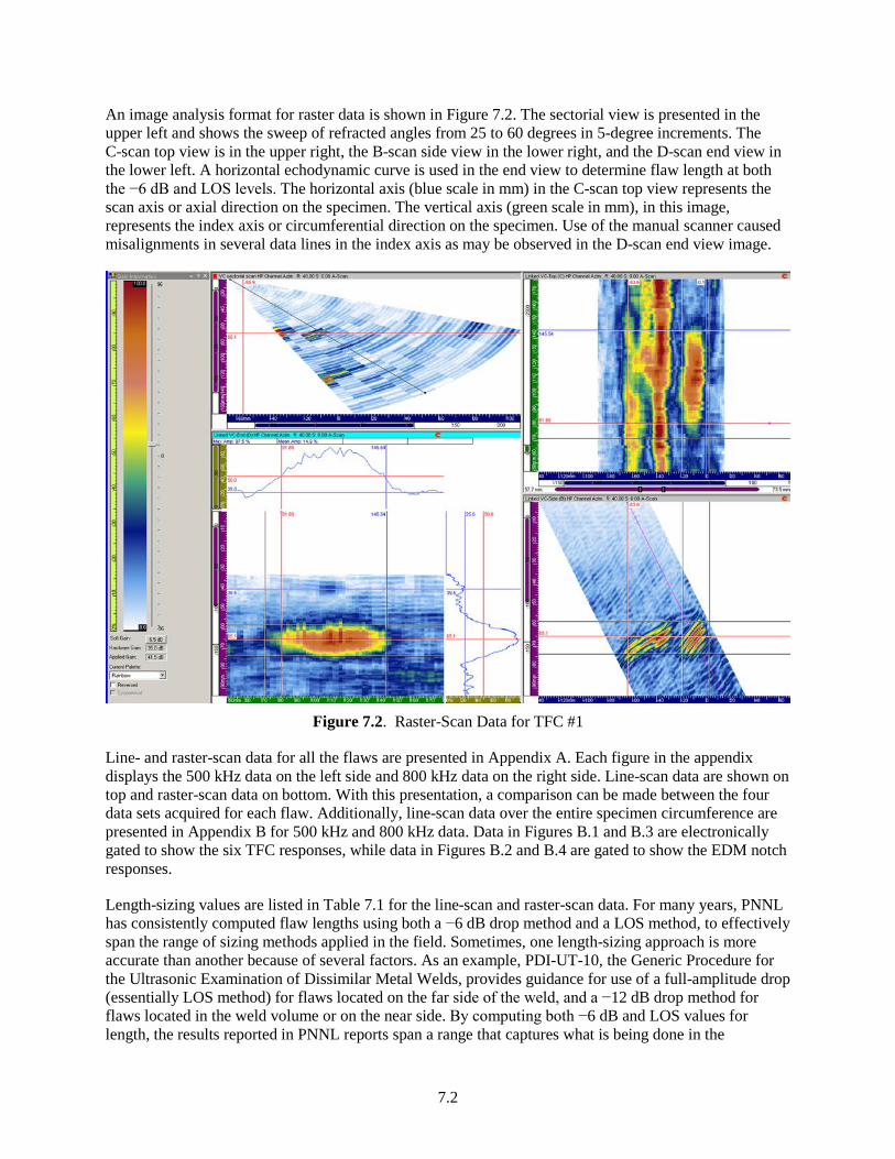
An image analysis format for raster data is shown in Figure 7.2. The sectorial view is presented in the upper left and shows the sweep of refracted angles from 25 to 60 degrees in 5-degree increments. The C-scan top view is in the upper right, the B-scan side view in the lower right, and the D-scan end view in the lower left. A horizontal echodynamic curve is used in the end view to determine flaw length at both the −6 dB and LOS levels. The horizontal axis (blue scale in mm) in the C-scan top view represents the scan axis or axial direction on the specimen. The vertical axis (green scale in mm), in this image, represents the index axis or circumferential direction on the specimen. Use of the manual scanner caused misalignments in several data lines in the index axis as may be observed in the D-scan end view image.
Figure 7.2. Raster-Scan Data for TFC #1
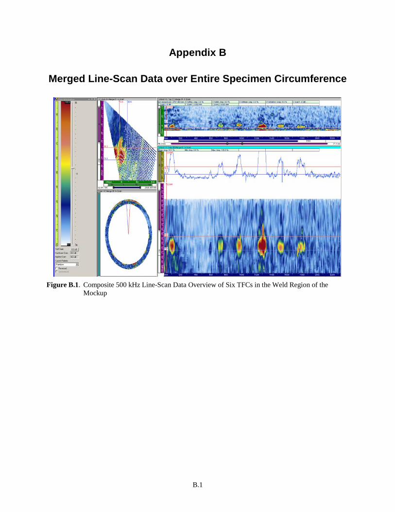
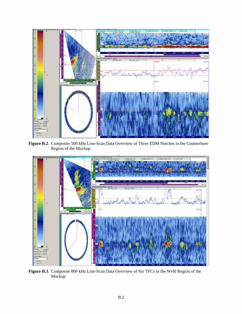
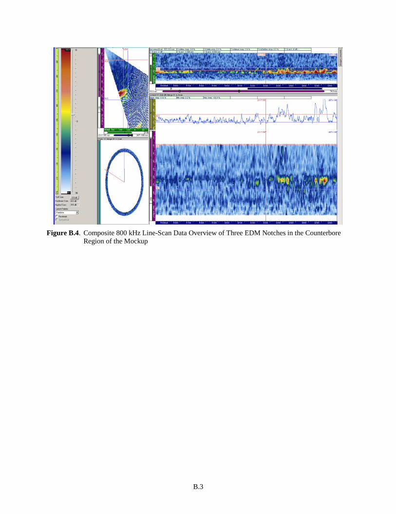
Line- and raster-scan data for all the flaws are presented in Appendix A. Each figure in the appendix displays the 500 kHz data on the left side and 800 kHz data on the right side. Line-scan data are shown on top and raster-scan data on bottom. With this presentation, a comparison can be made between the four data sets acquired for each flaw. Additionally, line-scan data over the entire specimen circumference are presented in Appendix B for 500 kHz and 800 kHz data. Data in Figures B.1 and B.3 are electronically gated to show the six TFC responses, while data in Figures B.2 and B.4 are gated to show the EDM notch responses.
Length-sizing values are listed in Table 7.1 for the line-scan and raster-scan data. For many years, PNNL has consistently computed flaw lengths using both a −6 dB drop method and a LOS method, to effectively span the range of sizing methods applied in the field. Sometimes, one length-sizing approach is more accurate than another because of several factors. As an example, PDI-UT-10, the Generic Procedure for the Ultrasonic Examination of Dissimilar Metal Welds, provides guidance for use of a full-amplitude drop (essentially LOS method) for flaws located on the far side of the weld, and a −12 dB drop method for flaws located in the weld volume or on the near side. By computing both −6 dB and LOS values for length, the results reported in PNNL reports span a range that captures what is being done in the
7.3
laboratory, at PDI, and in the field for flaw length sizing. By reporting this information, the reader can better understand potential variability in sizing results because of factors such as material, flaw type, location, etc.
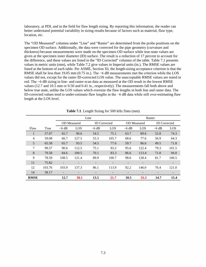
The “OD Measured” columns under “Line” and “Raster” are determined from the probe positions on the specimen OD surface. Additionally, the data were corrected for the pipe geometry (curvature and thickness) because measurements were made on the specimen OD surface while true-state values are given at the specimen inner diameter (ID) surface. The result is a reduction of 17 percent to account for the difference, and these values are listed in the “ID Corrected” columns of the table. Table 7.1 presents values in metric units (mm), while Table 7.2 give values in Imperial units (in.). The RMSE values are listed at the bottom of each table. Per ASME, Section XI, the length-sizing acceptance criterion is that the RMSE shall be less than 19.05 mm (0.75 in.). The −6 dB measurements met the criterion while the LOS values did not, except for the raster ID-corrected LOS value. The unacceptable RMSE values are noted in red. The −6 dB sizing in line- and raster-scan data as measured at the OD result in the lowest RMSE values (12.7 and 10.5 mm or 0.50 and 0.41 in., respectively). The measurements fall both above and below true state, unlike the LOS values which oversize the flaw lengths in both line and raster data. The ID-corrected values tend to under-estimate flaw lengths in the −6 dB data while still over-estimating flaw length at the LOS level.
Table 7.1. Length Sizing for 500 kHz Data (mm)
Line Raster
OD Measured ID Corrected OD Measured ID Corrected Flaw True −6 dB LOS −6 dB LOS −6 dB LOS −6 dB LOS
1 57.07 65.7 90.6 54.5 75.1 63.7 89.6 52.8 74.3 4 59.08 66.7 127.5 55.3 105.7 68.6 77.6 56.9 64.3 5 65.58 65.7 93.5 54.5 77.6 59.7 86.6 49.5 71.8 7 99.57 90.6 112.5 75.1 93.2 95.6 122.4 79.3 101.5 8 79.58 84.6 100.5 70.1 83.3 86.6 113.4 71.8 94.0 9 78.59 108.5 121.4 89.9 100.7 98.6 128.4 81.7 106.5
11 75.82 - - - - - - - - 12 103.76 103.9 137.3 86.1 113.9 92.2 146.0 76.4 121.0 14 58.17 - - - - - - - -
RMSE 12.7 38.1 13.5 21.7 10.5 33.3 14.7 15.4
7.4
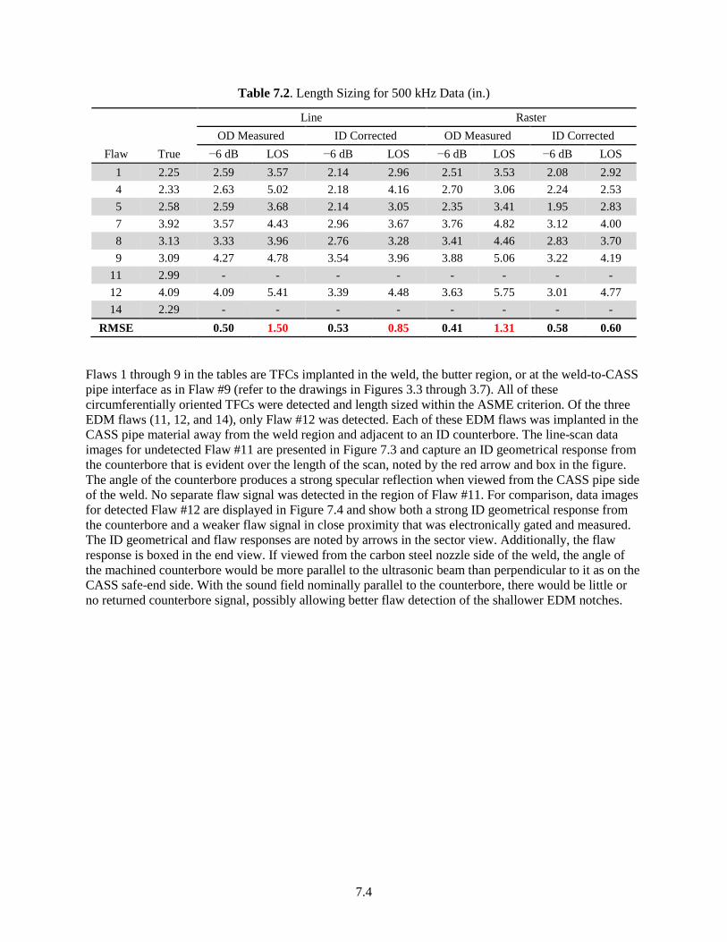
Table 7.2. Length Sizing for 500 kHz Data (in.)
Line Raster
OD Measured ID Corrected OD Measured ID Corrected Flaw True −6 dB LOS −6 dB LOS −6 dB LOS −6 dB LOS
1 2.25 2.59 3.57 2.14 2.96 2.51 3.53 2.08 2.92 4 2.33 2.63 5.02 2.18 4.16 2.70 3.06 2.24 2.53 5 2.58 2.59 3.68 2.14 3.05 2.35 3.41 1.95 2.83 7 3.92 3.57 4.43 2.96 3.67 3.76 4.82 3.12 4.00 8 3.13 3.33 3.96 2.76 3.28 3.41 4.46 2.83 3.70 9 3.09 4.27 4.78 3.54 3.96 3.88 5.06 3.22 4.19
11 2.99 - - - - - - - - 12 4.09 4.09 5.41 3.39 4.48 3.63 5.75 3.01 4.77 14 2.29 - - - - - - - -
RMSE 0.50 1.50 0.53 0.85 0.41 1.31 0.58 0.60
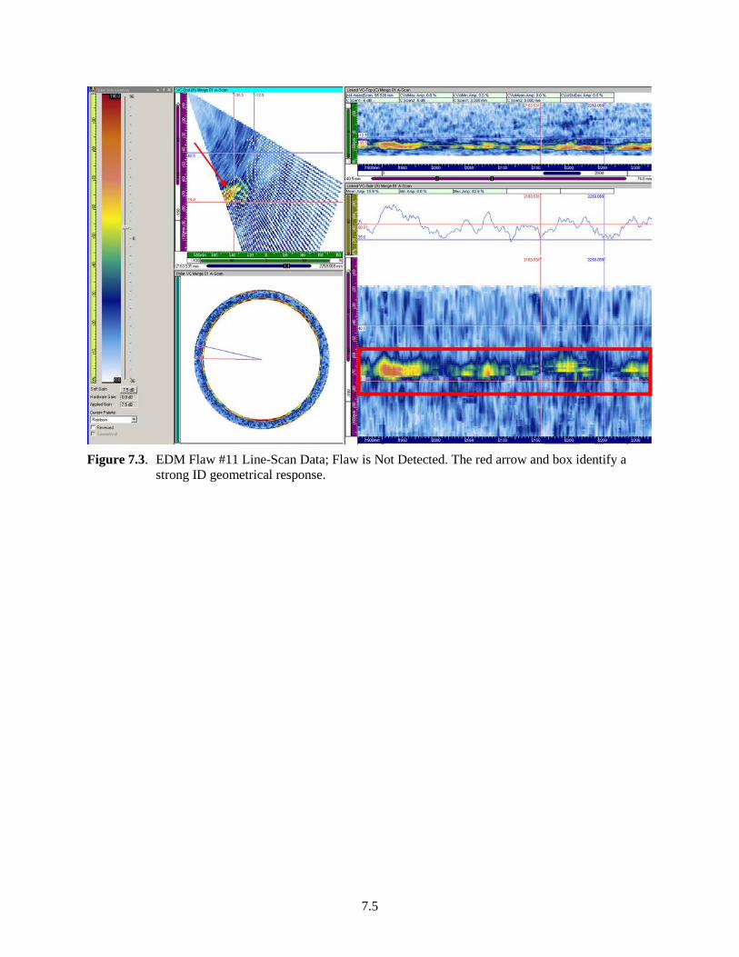
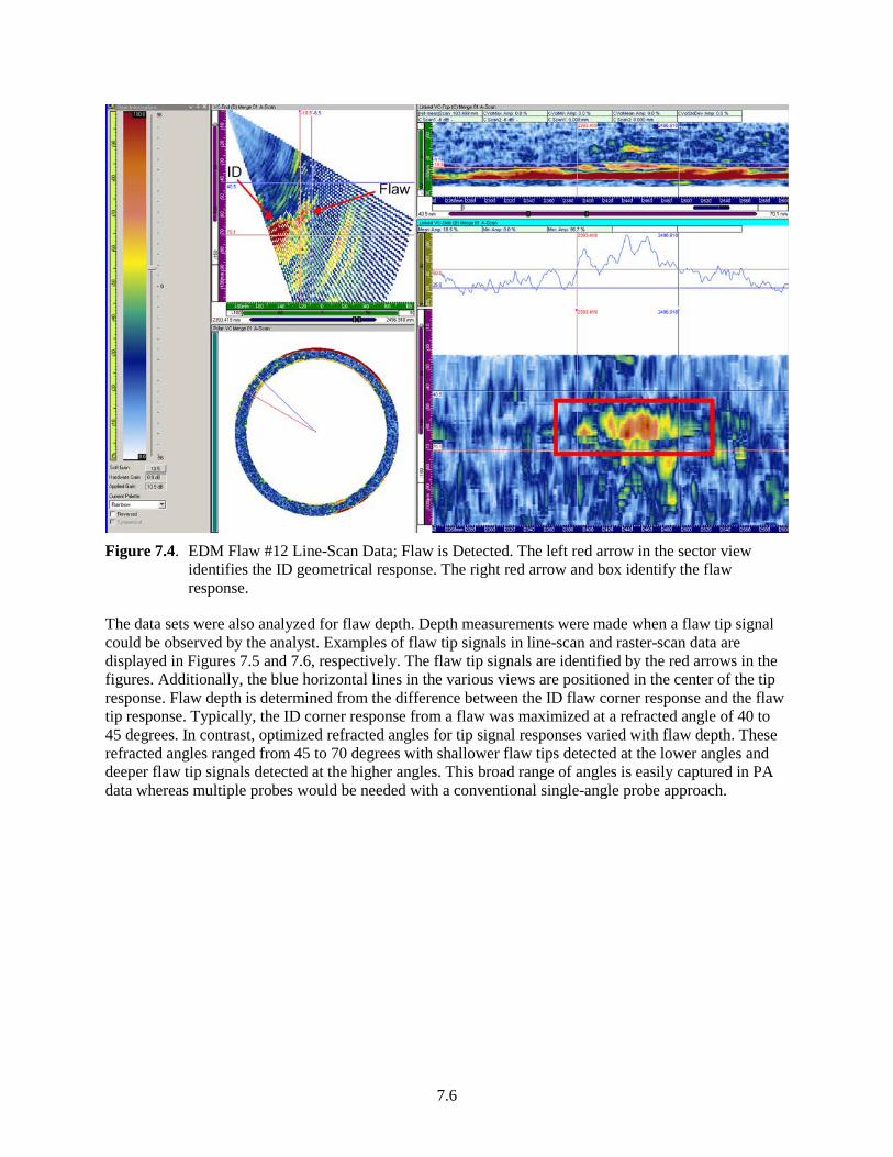
Flaws 1 through 9 in the tables are TFCs implanted in the weld, the butter region, or at the weld-to-CASS pipe interface as in Flaw #9 (refer to the drawings in Figures 3.3 through 3.7). All of these circumferentially oriented TFCs were detected and length sized within the ASME criterion. Of the three EDM flaws (11, 12, and 14), only Flaw #12 was detected. Each of these EDM flaws was implanted in the CASS pipe material away from the weld region and adjacent to an ID counterbore. The line-scan data images for undetected Flaw #11 are presented in Figure 7.3 and capture an ID geometrical response from the counterbore that is evident over the length of the scan, noted by the red arrow and box in the figure. The angle of the counterbore produces a strong specular reflection when viewed from the CASS pipe side of the weld. No separate flaw signal was detected in the region of Flaw #11. For comparison, data images for detected Flaw #12 are displayed in Figure 7.4 and show both a strong ID geometrical response from the counterbore and a weaker flaw signal in close proximity that was electronically gated and measured. The ID geometrical and flaw responses are noted by arrows in the sector view. Additionally, the flaw response is boxed in the end view. If viewed from the carbon steel nozzle side of the weld, the angle of the machined counterbore would be more parallel to the ultrasonic beam than perpendicular to it as on the CASS safe-end side. With the sound field nominally parallel to the counterbore, there would be little or no returned counterbore signal, possibly allowing better flaw detection of the shallower EDM notches.
7.5
Figure 7.3. EDM Flaw #11 Line-Scan Data; Flaw is Not Detected. The red arrow and box identify a
strong ID geometrical response.
7.6
Figure 7.4. EDM Flaw #12 Line-Scan Data; Flaw is Detected. The left red arrow in the sector view
identifies the ID geometrical response. The right red arrow and box identify the flaw response.
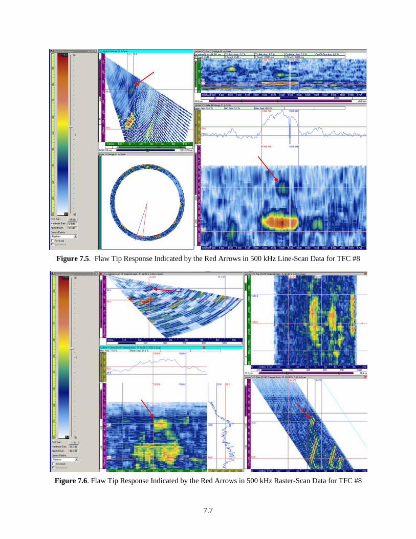
The data sets were also analyzed for flaw depth. Depth measurements were made when a flaw tip signal could be observed by the analyst. Examples of flaw tip signals in line-scan and raster-scan data are displayed in Figures 7.5 and 7.6, respectively. The flaw tip signals are identified by the red arrows in the figures. Additionally, the blue horizontal lines in the various views are positioned in the center of the tip response. Flaw depth is determined from the difference between the ID flaw corner response and the flaw tip response. Typically, the ID corner response from a flaw was maximized at a refracted angle of 40 to 45 degrees. In contrast, optimized refracted angles for tip signal responses varied with flaw depth. These refracted angles ranged from 45 to 70 degrees with shallower flaw tips detected at the lower angles and deeper flaw tip signals detected at the higher angles. This broad range of angles is easily captured in PA data whereas multiple probes would be needed with a conventional single-angle probe approach.
7.7
Figure 7.5. Flaw Tip Response Indicated by the Red Arrows in 500 kHz Line-Scan Data for TFC #8
Figure 7.6. Flaw Tip Response Indicated by the Red Arrows in 500 kHz Raster-Scan Data for TFC #8
7.8
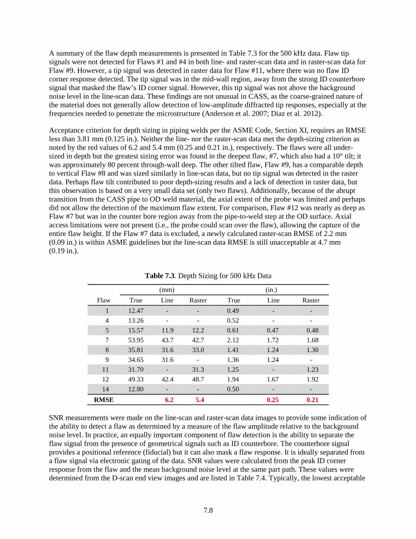
A summary of the flaw depth measurements is presented in Table 7.3 for the 500 kHz data. Flaw tip signals were not detected for Flaws #1 and #4 in both line- and raster-scan data and in raster-scan data for Flaw #9. However, a tip signal was detected in raster data for Flaw #11, where there was no flaw ID corner response detected. The tip signal was in the mid-wall region, away from the strong ID counterbore signal that masked the flaw’s ID corner signal. However, this tip signal was not above the background noise level in the line-scan data. These findings are not unusual in CASS, as the coarse-grained nature of the material does not generally allow detection of low-amplitude diffracted tip responses, especially at the frequencies needed to penetrate the microstructure (Anderson et al. 2007; Diaz et al. 2012).
Acceptance criterion for depth sizing in piping welds per the ASME Code, Section XI, requires an RMSE less than 3.81 mm (0.125 in.). Neither the line- nor the raster-scan data met the depth-sizing criterion as noted by the red values of 6.2 and 5.4 mm (0.25 and 0.21 in.), respectively. The flaws were all under-sized in depth but the greatest sizing error was found in the deepest flaw, #7, which also had a 10° tilt; it was approximately 80 percent through-wall deep. The other tilted flaw, Flaw #9, has a comparable depth to vertical Flaw #8 and was sized similarly in line-scan data, but no tip signal was detected in the raster data. Perhaps flaw tilt contributed to poor depth-sizing results and a lack of detection in raster data, but this observation is based on a very small data set (only two flaws). Additionally, because of the abrupt transition from the CASS pipe to OD weld material, the axial extent of the probe was limited and perhaps did not allow the detection of the maximum flaw extent. For comparison, Flaw #12 was nearly as deep as Flaw #7 but was in the counter bore region away from the pipe-to-weld step at the OD surface. Axial access limitations were not present (i.e., the probe could scan over the flaw), allowing the capture of the entire flaw height. If the Flaw #7 data is excluded, a newly calculated raster-scan RMSE of 2.2 mm (0.09 in.) is within ASME guidelines but the line-scan data RMSE is still unacceptable at 4.7 mm (0.19 in.).
Table 7.3. Depth Sizing for 500 kHz Data
(mm) (in.) Flaw True Line Raster True Line Raster
1 12.47 - - 0.49 - - 4 13.26 - - 0.52 - - 5 15.57 11.9 12.2 0.61 0.47 0.48 7 53.95 43.7 42.7 2.12 1.72 1.68 8 35.81 31.6 33.0 1.41 1.24 1.30 9 34.65 31.6 - 1.36 1.24 -
11 31.70 - 31.3 1.25 - 1.23 12 49.33 42.4 48.7 1.94 1.67 1.92 14 12.80 - - 0.50 - -
RMSE 6.2 5.4 0.25 0.21
SNR measurements were made on the line-scan and raster-scan data images to provide some indication of the ability to detect a flaw as determined by a measure of the flaw amplitude relative to the background noise level. In practice, an equally important component of flaw detection is the ability to separate the flaw signal from the presence of geometrical signals such as ID counterbore. The counterbore signal provides a positional reference (fiducial) but it can also mask a flaw response. It is ideally separated from a flaw signal via electronic gating of the data. SNR values were calculated from the peak ID corner response from the flaw and the mean background noise level at the same part path. These values were determined from the D-scan end view images and are listed in Table 7.4. Typically, the lowest acceptable
7.9
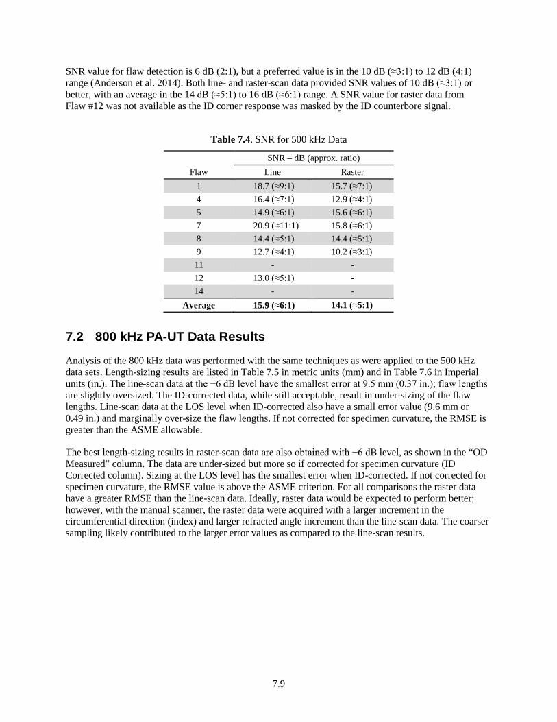
SNR value for flaw detection is 6 dB (2:1), but a preferred value is in the 10 dB (≈3:1) to 12 dB (4:1) range (Anderson et al. 2014). Both line- and raster-scan data provided SNR values of 10 dB (≈3:1) or better, with an average in the 14 dB (≈5:1) to 16 dB (≈6:1) range. A SNR value for raster data from Flaw #12 was not available as the ID corner response was masked by the ID counterbore signal.
Table 7.4. SNR for 500 kHz Data
SNR – dB (approx. ratio) Flaw Line Raster
1 18.7 (≈9:1) 15.7 (≈7:1) 4 16.4 (≈7:1) 12.9 (≈4:1) 5 14.9 (≈6:1) 15.6 (≈6:1) 7 20.9 (≈11:1) 15.8 (≈6:1) 8 14.4 (≈5:1) 14.4 (≈5:1) 9 12.7 (≈4:1) 10.2 (≈3:1) 11 - - 12 13.0 (≈5:1) - 14 - -
Average 15.9 (≈6:1) 14.1 (≈5:1)
7.2 800 kHz PA-UT Data Results
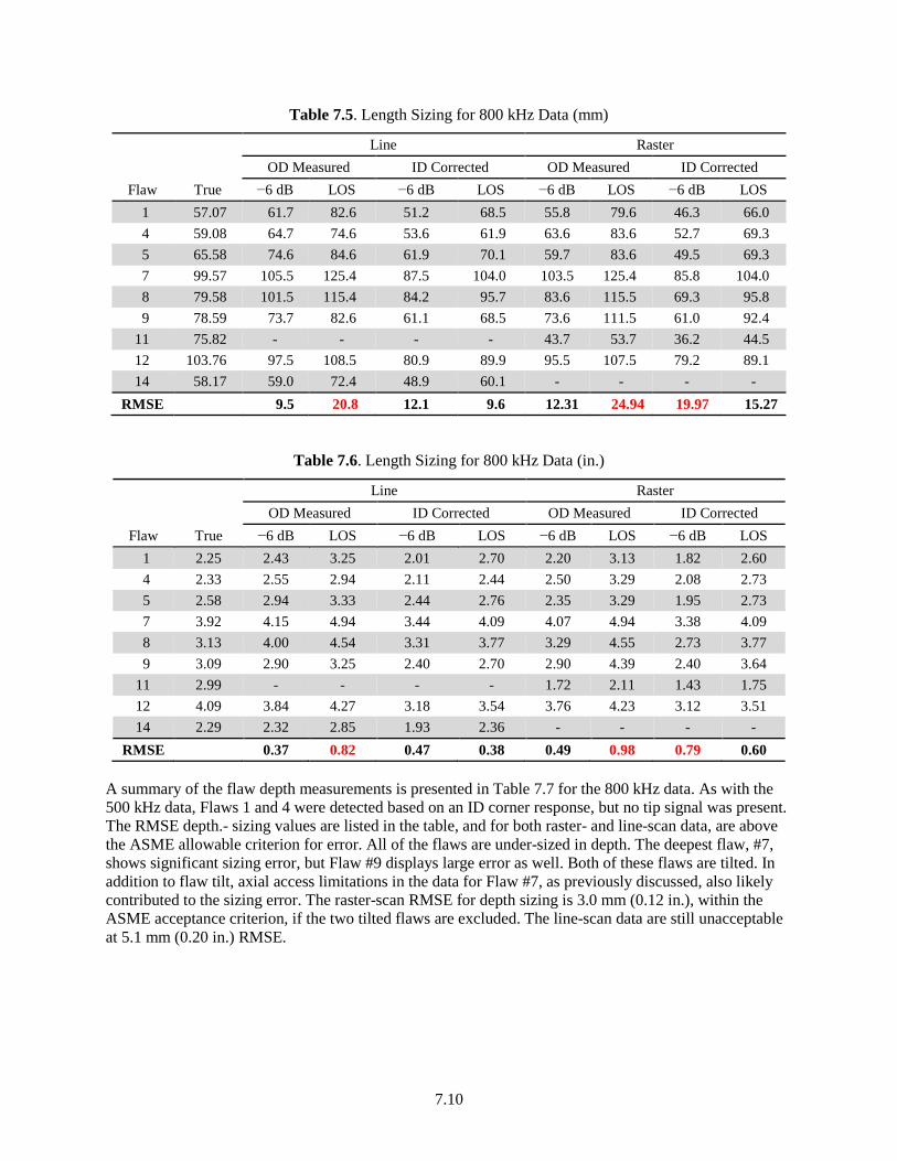
Analysis of the 800 kHz data was performed with the same techniques as were applied to the 500 kHz data sets. Length-sizing results are listed in Table 7.5 in metric units (mm) and in Table 7.6 in Imperial units (in.). The line-scan data at the −6 dB level have the smallest error at 9.5 mm (0.37 in.); flaw lengths are slightly oversized. The ID-corrected data, while still acceptable, result in under-sizing of the flaw lengths. Line-scan data at the LOS level when ID-corrected also have a small error value (9.6 mm or 0.49 in.) and marginally over-size the flaw lengths. If not corrected for specimen curvature, the RMSE is greater than the ASME allowable.
The best length-sizing results in raster-scan data are also obtained with −6 dB level, as shown in the “OD Measured” column. The data are under-sized but more so if corrected for specimen curvature (ID Corrected column). Sizing at the LOS level has the smallest error when ID-corrected. If not corrected for specimen curvature, the RMSE value is above the ASME criterion. For all comparisons the raster data have a greater RMSE than the line-scan data. Ideally, raster data would be expected to perform better; however, with the manual scanner, the raster data were acquired with a larger increment in the circumferential direction (index) and larger refracted angle increment than the line-scan data. The coarser sampling likely contributed to the larger error values as compared to the line-scan results.
7.10
Table 7.5. Length Sizing for 800 kHz Data (mm)
Line Raster
OD Measured ID Corrected OD Measured ID Corrected Flaw True −6 dB LOS −6 dB LOS −6 dB LOS −6 dB LOS
1 57.07 61.7 82.6 51.2 68.5 55.8 79.6 46.3 66.0 4 59.08 64.7 74.6 53.6 61.9 63.6 83.6 52.7 69.3 5 65.58 74.6 84.6 61.9 70.1 59.7 83.6 49.5 69.3 7 99.57 105.5 125.4 87.5 104.0 103.5 125.4 85.8 104.0 8 79.58 101.5 115.4 84.2 95.7 83.6 115.5 69.3 95.8 9 78.59 73.7 82.6 61.1 68.5 73.6 111.5 61.0 92.4
11 75.82 - - - - 43.7 53.7 36.2 44.5 12 103.76 97.5 108.5 80.9 89.9 95.5 107.5 79.2 89.1 14 58.17 59.0 72.4 48.9 60.1 - - - -
RMSE 9.5 20.8 12.1 9.6 12.31 24.94 19.97 15.27
Table 7.6. Length Sizing for 800 kHz Data (in.)
Line Raster
OD Measured ID Corrected OD Measured ID Corrected Flaw True −6 dB LOS −6 dB LOS −6 dB LOS −6 dB LOS
1 2.25 2.43 3.25 2.01 2.70 2.20 3.13 1.82 2.60 4 2.33 2.55 2.94 2.11 2.44 2.50 3.29 2.08 2.73 5 2.58 2.94 3.33 2.44 2.76 2.35 3.29 1.95 2.73 7 3.92 4.15 4.94 3.44 4.09 4.07 4.94 3.38 4.09 8 3.13 4.00 4.54 3.31 3.77 3.29 4.55 2.73 3.77 9 3.09 2.90 3.25 2.40 2.70 2.90 4.39 2.40 3.64
11 2.99 - - - - 1.72 2.11 1.43 1.75 12 4.09 3.84 4.27 3.18 3.54 3.76 4.23 3.12 3.51 14 2.29 2.32 2.85 1.93 2.36 - - - -
RMSE 0.37 0.82 0.47 0.38 0.49 0.98 0.79 0.60
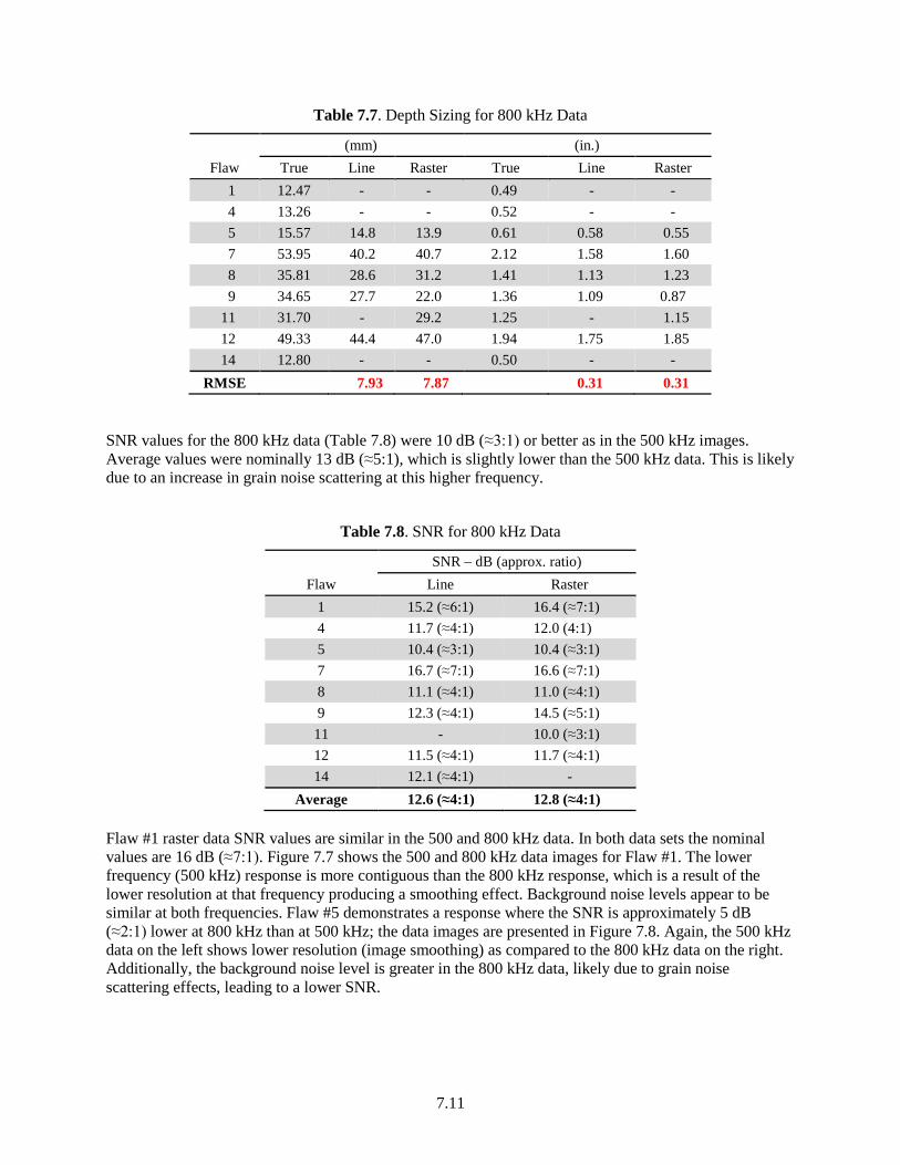
A summary of the flaw depth measurements is presented in Table 7.7 for the 800 kHz data. As with the 500 kHz data, Flaws 1 and 4 were detected based on an ID corner response, but no tip signal was present. The RMSE depth.- sizing values are listed in the table, and for both raster- and line-scan data, are above the ASME allowable criterion for error. All of the flaws are under-sized in depth. The deepest flaw, #7, shows significant sizing error, but Flaw #9 displays large error as well. Both of these flaws are tilted. In addition to flaw tilt, axial access limitations in the data for Flaw #7, as previously discussed, also likely contributed to the sizing error. The raster-scan RMSE for depth sizing is 3.0 mm (0.12 in.), within the ASME acceptance criterion, if the two tilted flaws are excluded. The line-scan data are still unacceptable at 5.1 mm (0.20 in.) RMSE.
7.11
Table 7.7. Depth Sizing for 800 kHz Data
(mm) (in.) Flaw True Line Raster True Line Raster
1 12.47 - - 0.49 - - 4 13.26 - - 0.52 - - 5 15.57 14.8 13.9 0.61 0.58 0.55 7 53.95 40.2 40.7 2.12 1.58 1.60 8 35.81 28.6 31.2 1.41 1.13 1.23 9 34.65 27.7 22.0 1.36 1.09 0.87
11 31.70 - 29.2 1.25 - 1.15 12 49.33 44.4 47.0 1.94 1.75 1.85 14 12.80 - - 0.50 - -
RMSE 7.93 7.87 0.31 0.31
SNR values for the 800 kHz data (Table 7.8) were 10 dB (≈3:1) or better as in the 500 kHz images. Average values were nominally 13 dB (≈5:1), which is slightly lower than the 500 kHz data. This is likely due to an increase in grain noise scattering at this higher frequency.
Table 7.8. SNR for 800 kHz Data
SNR – dB (approx. ratio) Flaw Line Raster
1 15.2 (≈6:1) 16.4 (≈7:1) 4 11.7 (≈4:1) 12.0 (4:1) 5 10.4 (≈3:1) 10.4 (≈3:1) 7 16.7 (≈7:1) 16.6 (≈7:1) 8 11.1 (≈4:1) 11.0 (≈4:1) 9 12.3 (≈4:1) 14.5 (≈5:1) 11 - 10.0 (≈3:1) 12 11.5 (≈4:1) 11.7 (≈4:1) 14 12.1 (≈4:1) -
Average 12.6 (≈4:1) 12.8 (≈4:1)
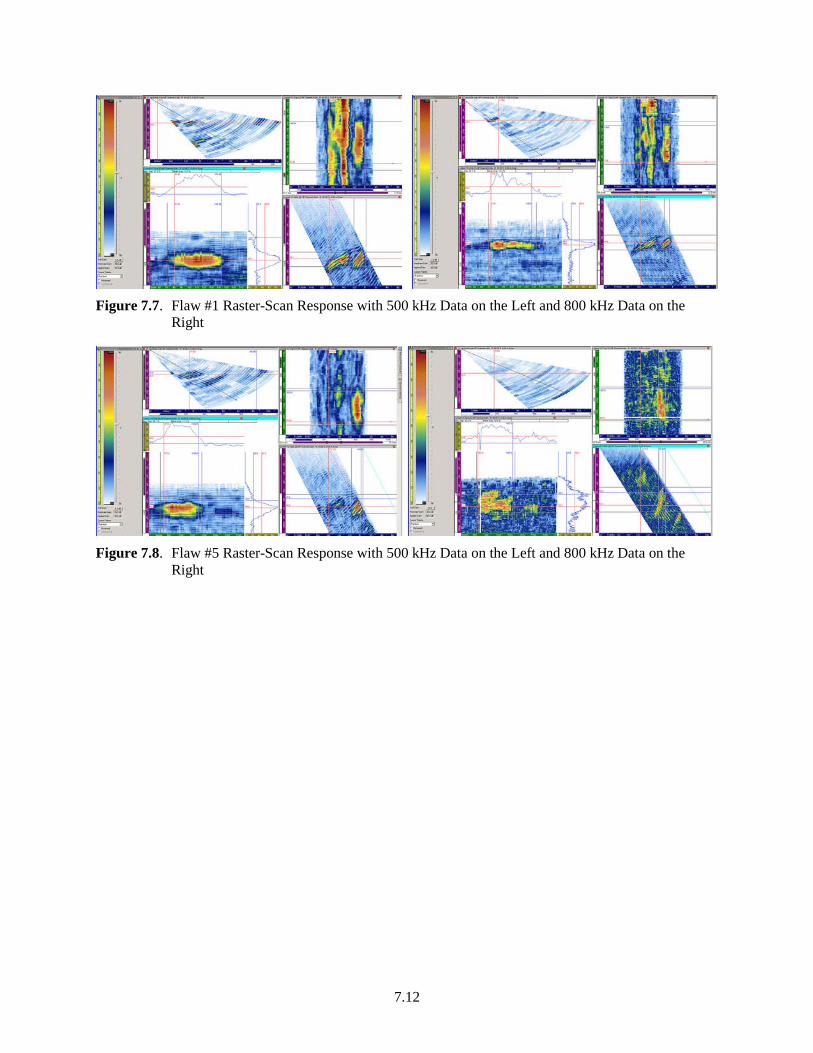
Flaw #1 raster data SNR values are similar in the 500 and 800 kHz data. In both data sets the nominal values are 16 dB (≈7:1). Figure 7.7 shows the 500 and 800 kHz data images for Flaw #1. The lower frequency (500 kHz) response is more contiguous than the 800 kHz response, which is a result of the lower resolution at that frequency producing a smoothing effect. Background noise levels appear to be similar at both frequencies. Flaw #5 demonstrates a response where the SNR is approximately 5 dB (≈2:1) lower at 800 kHz than at 500 kHz; the data images are presented in Figure 7.8. Again, the 500 kHz data on the left shows lower resolution (image smoothing) as compared to the 800 kHz data on the right. Additionally, the background noise level is greater in the 800 kHz data, likely due to grain noise scattering effects, leading to a lower SNR.
7.12
Figure 7.7. Flaw #1 Raster-Scan Response with 500 kHz Data on the Left and 800 kHz Data on the
Right
Figure 7.8. Flaw #5 Raster-Scan Response with 500 kHz Data on the Left and 800 kHz Data on the
Right
8.1
8.0 Discussion and Conclusions
8.1 Discussion
The exercise to acquire manually encoded PA-UT data on a thick-section CASS DMW component and the corresponding data analyses conducted provided an opportunity to further the understanding of the challenges involved in the inspections of such components. While the mockup contained both axially and circumferentially oriented flaws, only the circumferentially oriented flaws were examined. The mockup was designed and fabricated to simulate a Port St. Lucie reactor coolant system elbow/pipe-to-safe end configuration. It contained both implanted TFCs and EDM notches. Encoded, manual scan data were acquired only from the CASS side of the weld.
Six TFCs were implanted in the weld/butter region during the specimen fabrication process and were all detected by line and raster scans at 500 and 800 kHz. The three EDM notches were placed in the CASS pipe material away from the weld/butter region. Exact axial position information was not given, but the drawings show the EDM notches were in close proximity to an ID counterbore. It is likely that the strong ID counterbore signal masked the weaker ID corner response from two of the three EDM notches in the 500 kHz data and in some of the 800 kHz data as well. The deepest EDM notch, #12, approximately 80% through-wall and 103.8 mm (4.1 in.) long, was detected in all scans, however. Additionally, the 800 kHz data improved certain flaw detection in that EDM notch #11 was detected in the raster-scan and EDM notch #14 was detected in line-scan data.
Length-sizing accuracy was assessed with RMSE calculations for all nine flaws for each frequency and scanning method. Sizing at a −6 dB level as measured at the specimen OD (i.e., not corrected for specimen curvature) gave the least error. Depending on probe frequency and scanning method the RMSE values were between 9.5 and 12.7 mm (0.37 and 0.50 in.). An alternative sizing criterion is based on end points measured at the LOS level or −12 dB and this technique oversized the flaw lengths. If corrected for pipe curvature, the LOS values were closer to true state but still oversized flaw lengths. Raster- and line-scan data at 500 and 800 kHz at the −6 dB level all met the ASME length-sizing criterion for a RMSE value of less than 19.05 mm (0.75 in.) whereas the LOS values did not. The 800 kHz data improved flaw detection in that Flaw #11 was detected in raster-scan data while it was not detected in the 500 kHz data.
Depth sizing was performed if a flaw tip-diffracted response was detected. Flaw tips were not detected for two TFCs and one EDM notch, all on the order of 12.7 mm (0.5 in.) in depth, in any of the data. Tip signals were detected for TFCs with depths of 15.6 mm (0.61 in.) and deeper in most all of the data (line and raster, 500 and 800 kHz). The exception was that a tip signal was not found in the 500 kHz raster data for tilted Flaw #9 at 34.7 mm (1.36 in.) deep. A tip signal from the deepest EDM notch (49.3 mm or 1.94 in.), Flaw #12, was found in all data sets while EDM notch Flaw #11 presented a tip signal only in the raster data and at both frequencies. Depth-sizing error values as measured by RMSE, 5.4 mm (0.21 in.) for 500 kHz data and 7.9 mm (0.31 in.) for 800 kHz data, were above the ASME Code criterion of less than 3.81 mm (0.125 in.). Flaw tilt and geometrical limitations on axial access to two flaws perhaps led to higher error values. If these data points were removed, the RMSE values for raster data were within the ASME criterion. It should be noted that non-detection of flaw tip responses is not unusual in CASS (Anderson et al. 2007; Diaz et al. 2012), as the coarse-grained nature of the material does not typically allow detection of low-amplitude signals, such as would be presented by these type of diffracted sound patterns. This is especially true at the frequencies employed in this study, which are needed to penetrate the microstructure. Thus, UT methods to accurately depth-size these flaws remain as yet undeveloped. Other, non-standard depth-sizing methods such as LOS, full matrix capture, and/or non-linear acoustic post-processing techniques could be explored to assess their potential for providing
8.2
through-wall depth information of flaws when detected in CASS. Flaw depth-sizing may ultimately present a problem for field examinations of CASS piping, but this issue was beyond the scope of the work presented in this report.
Signal-to-noise values for the 500 kHz data were nominally 16 dB (≈6:1) for line-scan data and 14 dB (≈5:1) for raster data. The SNR values in the 800 kHz data were approximately 12.7 dB (≈4:1), for both line and raster data. While the 800 kHz data provide better resolution for sizing, there is typically an increase in grain noise leading to the lower SNR value as compared to the 500 kHz data.
Typically, raster-scan data are expected to provide better flaw characterization; however, the use of a manual scanner resulted in coarser resolutions in the index axis, and the sweep of refracted angles during raster scans was at higher angular increments than line scans. These variables likely contributed to the mixed results in that raster data did not always enhance the flaw characterization when compared to line-scan data.
8.2 Conclusions • Flaw Detection
– All six implanted TFCs were detected in all data sets (500k Hz, 800 kHz, line and raster)
– EDM notches, Flaws #11 and 14, were not detected in 500 kHz data but were detected in 800 kHz data—raster-scan data for Flaw #11 and line-scan data for Flaw #14, respectively
– Flaw placement in specimen axial position affects flaw detection
○ Shallow to deep (approximately 20–80% through-wall) TFCs were implanted in the weld and butter regions—all were detected
○ Shallow to mid-wall EDM notches axially positioned near the ID counterbore were less likely to be detected, because data were acquired from the CASS side that produced a strong reflection from the counterbore (pipe side or near side in this specimen) that masked certain EDMs
○ Data, if acquired from the carbon steel nozzle side, may improve flaw detection of missed EDM notches
• Flaw Depth Sizing
– 500 kHz data had no detected tip signals for TFCs #1, #4, and raster data #9; also EDM notch #11 line data and EDM notch #14
– 800 kHz data showed the ability to detect a tip for TFC #9 in the raster data, otherwise results were similar to the 500 kHz data
• 500 kHz and 800 kHz Data Comparison
– 800 kHz improved flaw detection (based on two notches becoming more evident at this frequency in this particular CASS material)
– Greater flaw-sizing resolution at 800 kHz but also greater noise [nominally 13 dB (≈5:1) compared to 15 dB (≈6:1) SNR]
• ASME requirements for length-sizing error were met
• ASME requirements for depth-sizing error were not met, possibly due to flaw tilt and limited axial access to the flaw due to specimen OD geometry at the weld.
9.1
9.0 References
Anderson MT, SL Crawford, SE Cumblidge, KM Denslow, AA Diaz and SR Doctor. 2007. Assessment of Crack Detection in Heavy-Walled Cast Stainless Steel Piping Welds Using Advanced Low-Frequency Ultrasonic Methods. NUREG/CR-6933, PNNL-16292, U.S. Nuclear Regulatory Commission, Washington, D.C. ADAMS Accession No. ML071020410.
Anderson MT, AA Diaz, AD Cinson, SL Crawford, MS Prowant and SR Doctor. 2014. Final Assessment of Manual Ultrasonic Examinations Applied to Detect Flaws in Primary System Dissimilar Metal Welds at North Anna Power Station. PNNL-22553, Pacific Northwest National Laboratory, Richland, Washington. ADAMS Accession No. ML14080A002.
Diaz AA, AD Cinson, SL Crawford, R Mathews, TL Moran, MS Prowant and MT Anderson. 2012. An Evaluation of Ultrasonic Phased Array Testing for Cast Austenitic Stainless Steel Pressurizer Surge Line Piping Welds. NUREG/CR-7122, PNNL-19497, Pacific Northwest National Laboratory, Richland, Washington. ADAMS Accession No. ML12087A061 and ML12087A063.
Diaz AA, SR Doctor, BP Hildebrand, FA Simonen, GJ Schuster, ES Andersen, GP McDonald and RD Hasse. 1998. Evaluation of Ultrasonic Inspection Techniques for Coarse-Grained Materials. NUREG/CR-6594, PNNL-11171, U.S. Nuclear Regulatory Commission, Washington, D.C.
Diaz AA, RV Harris Jr. and SR Doctor. 2008. Field Evaluation of Low-Frequency SAFT-UT on Cast Stainless Steel and Dissimilar Metal Weld Components. NUREG/CR-6984, PNNL-14374, U.S. Nuclear Regulatory Commission, Washington, D.C.
Doctor SR, GJ Schuster, LD Reid and TE Hall. 1996. Real-Time 3-D SAFT-UT Evaluation and Validation. NUREG/CR-6344, PNNL-10571, U.S. Nuclear Regulatory Commission, Washington, D.C.
Ensminger D and LJ Bond. 2011. "Medical Applications of Ultrasonic Energy." In Ultrasonics: Fundamentals, Technology and Applications, Third Edition (Revised and Expanded). CRC Press, Boca Raton, Florida.
Goebbels K. 1994. Materials Characterization for Process Control and Product Conformity. CRC Press, Boca Raton, Florida.
Hall TE, LD Reid and SR Doctor. 1988. The SAFT-UT Real-Time Inspection System - Operational Principles and Implementation. NUREG/CR-5075, PNNL-6413, U.S. Nuclear Regulatory Commission, Washington, D.C.
Szilard J, Ed. 1982. Ultrasonic Testing Non-conventional Testing Techniques. John Wiley & Sons, New York. Chapters 1 and 6.
Thompson RB, FJ Margetan, P Haldipur, L Yu, A Li, P Panetta and H Wasan. 2008. "Scattering of Elastic Waves in Simple and Complex Polycrystals." Wave Motion 45:655-674.

Appendix A –
500 kHz and 800 kHz PA-UT Line-Scan and Raster-Scan Data Images

A.1
Appendix A
500 kHz and 800 kHz PA-UT Line-Scan and Raster-Scan Data Images
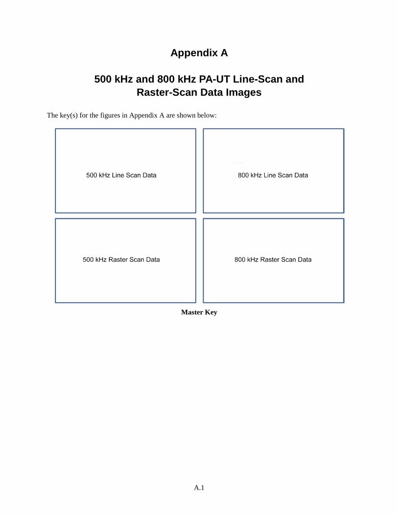
The key(s) for the figures in Appendix A are shown below:
Master Key
A.2
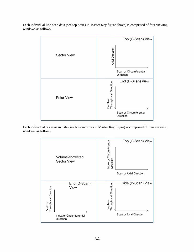
Each individual line-scan data (see top boxes in Master Key figure above) is comprised of four viewing windows as follows:
Each individual raster-scan data (see bottom boxes in Master Key figure) is comprised of four viewing windows as follows:
A.3
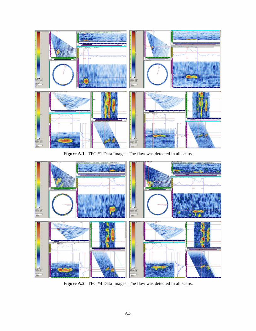
Figure A.1. TFC #1 Data Images. The flaw was detected in all scans.
Figure A.2. TFC #4 Data Images. The flaw was detected in all scans.
A.4
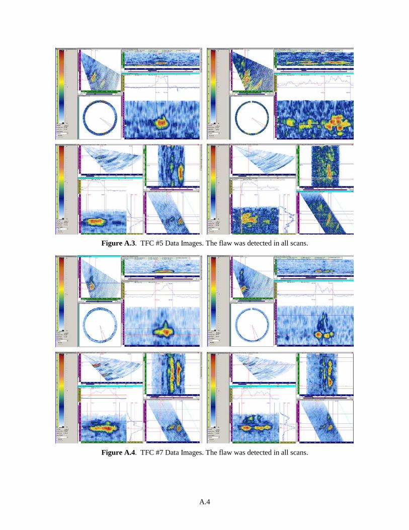
Figure A.3. TFC #5 Data Images. The flaw was detected in all scans.
Figure A.4. TFC #7 Data Images. The flaw was detected in all scans.
A.5
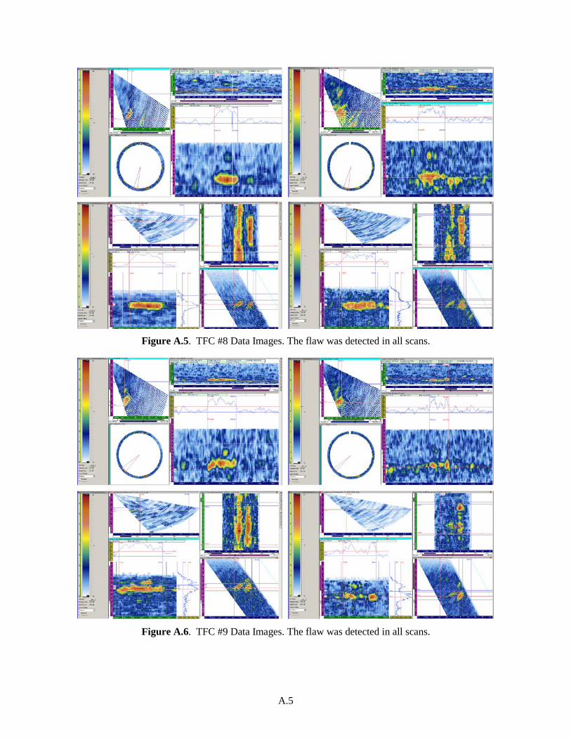
Figure A.5. TFC #8 Data Images. The flaw was detected in all scans.
Figure A.6. TFC #9 Data Images. The flaw was detected in all scans.
A.6
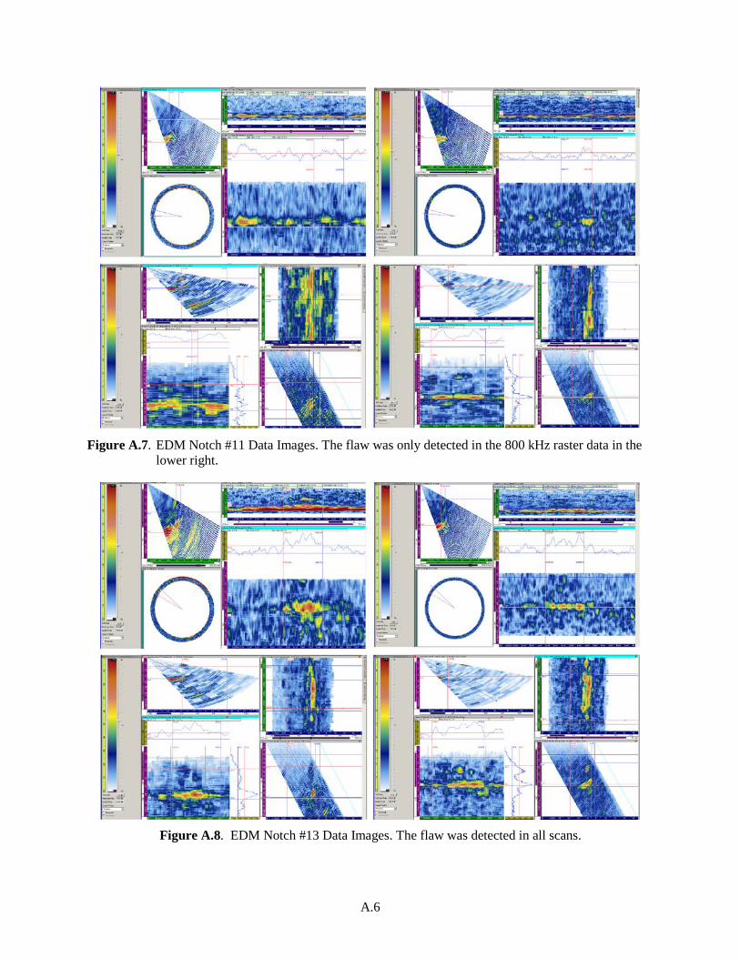
Figure A.7. EDM Notch #11 Data Images. The flaw was only detected in the 800 kHz raster data in the
lower right.
Figure A.8. EDM Notch #13 Data Images. The flaw was detected in all scans.
A.7
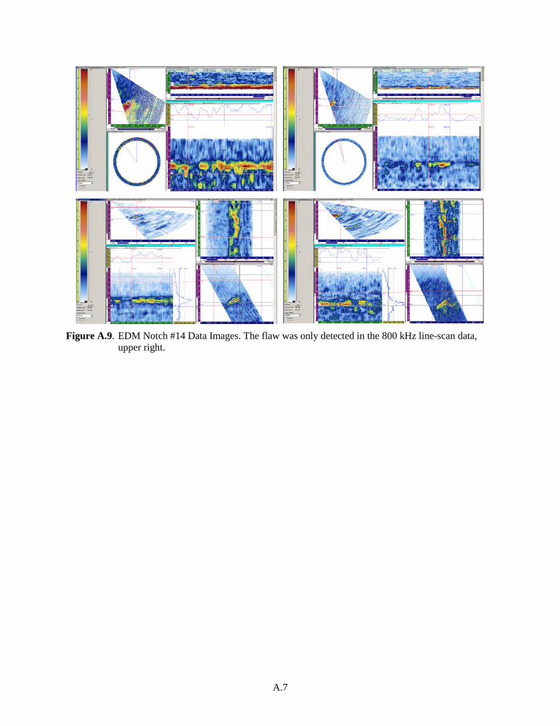
Figure A.9. EDM Notch #14 Data Images. The flaw was only detected in the 800 kHz line-scan data,
upper right.

Appendix B –
Merged Line-Scan Data over Entire Specimen Circumference

B.1
Appendix B
Merged Line-Scan Data over Entire Specimen Circumference
Figure B.1. Composite 500 kHz Line-Scan Data Overview of Six TFCs in the Weld Region of the
Mockup
B.2
Figure B.2. Composite 500 kHz Line-Scan Data Overview of Three EDM Notches in the Counterbore
Region of the Mockup
Figure B.3. Composite 800 kHz Line-Scan Data Overview of Six TFCs in the Weld Region of the
Mockup
B.3
Figure B.4. Composite 800 kHz Line-Scan Data Overview of Three EDM Notches in the Counterbore
Region of the Mockup


