Phase Transitions and Critical Phenomena: An Essay in Natural Philosophy (Thales to Onsager)

Prof. David A. Edwards Department of Mathematics University of Georgia Athens, Georgia 30602 http://www.math.uga.edu/~davide/ http://davidaedwards.tumblr.com/ dedwards@math.uga.edu

§1. Introduction. In this essay we will present a detailed analysis of the concepts and mathematics that underlie statistical mechanics. For a similar discussion of classical and quantum mechanics the reader is referred to [E-1] and [E-4]. For a similar discussion of quantum field theory the reader is referred to [E-2]. For a discussion of quantum geometrodynamics the reader is referred to [E-3] Scientific theories go through many stages in their development, some eventually reaching the stage at which one might say that "the only work left to be done is the computing of the next decimal." We shall call such theories climax theories in analogy with the notion of a climax forest (other analogies are also appropriate). A climax theory has two parts: one theoretical, which has become part of pure mathematics; and the other empirical, which somehow relates the mathematics to experience. The earliest example of a climax theory is Euclidean geometry. That such a development of geometry is even possible is not obvious. One can easily imagine an Egyptian geometer explaining to a Babylonian number theorist why geometry could never become a precise science like number theory because pyramids and other such bodies are intrinsically irregular and fuzzy (similar discussions occur often today between biologists and physicists). Archimedes' fundamental work showing that the four fundamental constants related to circles and spheres (C =αr, A = βr2 , S = ϒr 2, V= δr3 ) are all simply related (1/2α=β = 1/4ϒ= 3/4δ= π), together with his estimate that 3+10/71< π < 3+1/7 will serve for us as the paradigm of what science should be all about. Namely, rigorous derivation from a well defined theory yielding results that are empirically satisfactory. Gauss took geometry a step further by systematically developing non-Euclidean geometries and by attempting to determine which of these was empirically most adequate by measuring the sum of the angles of a triangle formed by three mountain tops. A further step was taken by Einstein who developed a four-dimensional Pseudo-Riemannian geometry of space-time and showed that it provided a better organizing principle of experience than the previous geometries. Thus, the only legitimate philosophical problems that we recognize in a mature scientific theory are the same ones that occur in geometry. Of course, raising a theory to the level at which it attains a Euclidean form requires a great effort. For example, while the Greeks (e.g., Aristotle) were very conscious of the importance of motion, they were only able to mathematically handle celestial mechanics (Ptolemy), and a full mathematical theory of dynamics was only successfully attained with Newton. Newton describes his program in the preface to his opus the Mathematical Principles of Natural Philosophy:

...therefore I offer this work as the mathematical principles of philosophy, for the whole burden of philosophy seems to consist in this - from the phenomena of motions to investigate the forces of nature, and then from these forces to demonstrate the other phenomena; and to this end the general propositions in the first and second books are directed. In the third book I give an example of this in the explication of the System of the World; for by the propositions mathematically demonstrated in the former books in the third I derive from the celestial phenomena the forces of gravity with which bodies tend to the sun and the several planets. Then from these forces by other propositions which are also mathematical, I deduce the motions of the planets, the comets, the moon, and the sea. I wish we could derive the rest of the phenomena of Nature by the same kind of reasoning from mechanical principles for I am induced by many reasons to suspect that they may all depend upon certain forces by which the particles of bodies, by some causes hitherto unknown, are either mutually impelled towards one another, and cohere in regular figures, or are repelled and recede from one another. These forces being unknown, philosophers have hitherto attempted the search of Nature in vain; but I hope the principles here laid down will afford some light either to this or some truer method of philosophy. [S] Newton clearly had a mighty vision. We will be surveying some of the progress made since Newton in deriving “the rest of the phenomena of Nature”.

§2. Statistical Mechanics.

§2.1 The Reductionist Program. At least from the time of the Greeks, it has been a dream of natural philosophers to establish a single model from which all of the phenomena of nature could be rigorously derived. One of the most enticing of such models was atomism. Under this hypothesis, a ground zero description of the world consists of atoms in motion in a void. All other phenomena are to be under stood as collective properties of the atoms. As originally understood, the atomic theory was a realistic theory - the atoms were real things independent of man. We will take a more idealistic approach. Namely, for us an atomic theory will entail the assumption of certain modes of perceiving. The rest of perception should then follow in a manner analogous to the way a long distance view of a Seurat painting follows from a close-up view. The point of atomic theories is to be able to derive the complex phenomena of appearances from simple initial assumptions. For example, one goal of atomic theory would be to derive the temperatures at which water freezes and boils. There were a number of atomic theories in antiquity, for example, those due to Leucippus, Democritus, Plato, Epicurus,-and Lucretius. These theories postulated a space which was either a passive void or an active plenum together with various fundamental particles. Plato's doctrine of geometrical atomism was certainly the most sophisticated. Consider the following passage from the Timaeus [S]. In the first place, then, it is of course obvious to anyone that fire, earth, water, and air are bodies; and all body has depth. Depth, moreover, must be bounded by surface; and every surface that is rectilinear is composed of triangles. Now all triangles are derived from two, each having one right angle and the other angles acute. Of these triangles, one has on either side the half of a right angle, the division of which is determined by equal sides (the right-angled isosceles); the other has unequal parts of a right angle allotted to unequal sides (the right-angled scalene). This we assume as the first beginning of fire and of the other bodies, following the account which combines likelihood with necessity; the principles yet more remote than

these are known to Heaven and to such men as Heaven favours. Now,the question to be determined is this: What are the most perfect bodies that can be constructed, four in number, unlike one another, but such that some can be generated out of one another by resolution? If we can hit upon the answer to this, we have the truth concerning the generation of earth and fire and of the bodies which stand as proportionals between them. For we shall concede to no one that there are visible bodies more perfect than these, each corresponding to a single type. We must do our best, then to construct the four types of body that are most perfect and declare that we have grasped the constitution of these things sufficiently for our purpose. Now, of the two triangles, the isosceles is of one type only; the scalene, of an endless number. Of this unlimited multitude we must choose the best, if we are to make a beginning on our own principles. Accordingly, if anyone can tell us of a better kind that he has chosen for the construction of these bodies, his will be the victory not of an enemy, but of a friend. For ourselves, however, we postulate as the best of these many triangles one kind, passing over all the rest; that, namely, a pair of which compose the equilateral triangle. The reason is too long a story; but if anyone should put the matter to the test and discover that it is not so, the prize is his with all good will. So much, then, for the choice of the two triangles, of which the bodies of fire and of the rest have been wrought: the one isosceles (the half-square),the other having the greater side triple in square of the lesser (the half-equilateral). We must now be more precise upon a point that was not clearly enough stated earlier. It appeared as though all the four kinds could pass through one another into one another; but this appearance is delusive: for the triangles we selected give rise to four types, and whereas three are constructed out of the triangle with unequal sides, the fourth alone is consttucted out of the isosceles. Hence it is not possible for all of them to pass into one another by resolution, many of the small forming a few of the greater and vice versa. But three of them can do this; for these are all composed of one triangle and when the larger bodies are broken up several small ones will be formed of the same triangles, taking on their proper figures; and again when several of the smaller bodies are dispersed into their triangles, the total number made up by them will produce a single new figure of larger size, belonging to a single body. So much for their passing into one another. The next thing to explain is, what sort of figure each body has, and the numbers that combine to compose it. First will come the construction of the simplest and smallest figure (the pyramid). Its element is the triangle whose hypotenuse is double of the shorter side in length. If a pair of such triangles are put together by the diagonal and this is node three times, the diagonals and the shorter sides resting on the same point as a centre, in this way a single equilateral triangle is formed of triangles six in number. If four equilateral triangles are put together, their plane angles meeting in groups of three make a single solid angle, namely the one (180°) that comes next after the most obtuse of plane angles. When four such angles are produced, the simplest solid figure is formed, whose property is to divide the whole circumference into equal and similar parts. A second body (the octahedron) is composed of the same (elementary) triangles when they are combined in a ,set of eight equilateral triangles, and yield a solid angle formed by four plane angles. With the production of six such solid angles the second body is complete. The third body (the icosahedron) is composed of one hundred and twenty of the elementary triangles fitted together, and of twelve solid angles, each contained by five equilateral triangular planes; and it has twenty facts which are equilateral triangles. Here one of the two elements, having generated these bodies has done its part. But the isosceles triangle went on to generate the fourth body, being put together in sets of four, with their right angles meeting at the centre, thus forming a single equilateral quadrangle. Six such quadrangles, joined together, produced eight solid angles, each composed by a set of three plane right

angles. The shape of the resulting body was cubical having six quadrangular equilateral planes as its faces [...] Let us next distribute the figures whose formation we have now described, among fire, earth, water and air. To earth let us assign the cubical figure; for of the four kinds earth is the most immobile and the most plactic of bodies. The figure whose bases are the most stable must best answer that description; and as a base, if we take the triangles we assumed at the outset, the face of the triangle with equal sides is by nature more stable than that of the triangle whose sides are unequal; and further, of the two equilateral surfaces respectively composed of the two triangles, the square is necessarily a more stable base than the triangle, both in its parts and as a whole. Accordingly we shall preserve the probability of our account, if we assign this figure to earth; and of the remainder the least mobile to water, the most mobile to fire, and the intermediate figure to air. Again, we shall assign the smallest body to fire, the largest to water, and the intermediate to air; and again the body with the sharpest angles to fire, the next to air, the third to water. Now, taking all these figures, the one with the fewest faces (pyramid) must be the most mobile, since it has the sharpest cutting edges and the sharpest points in every direction, and moreover the lightest, as being composed of the smallest number of similar parts; the second (octahedron) must stand second in these respects, the third (icosahedron), third. Hence, in accordance with genuine reasoning as well as probability, among the solid figures we have constructed, we may take the pyramid as the element or seed of fire; the second in order of generation (octahedron) as that of air; the third (icosahedron) as that of water. Now we must think of all these bodies as so small that a single body of any one of these kinds is invisible to us because of its smallness; though when a number are aggregated the masses of them can be seen. And with regard to their numbers, there motions, and their powers in general, we must suppose that the god adjusted them in due proportion, when he had brought them in every detail to the most exact perfection permitted by Necessity willingly complying with persuasion. Now, from all that we have said in the foregoing account concerning the kinds, the following would be the most probable description of the facts. Earth, when it meets with fire and is dissolved by its sharpness, would drift about - whether, when dissovled, it be enveloped in fire itself or in a mass of air or of water - until its own parts somewhere encounter one another, are fitted together and again become earth; for they can never pass into any other kind. But (I) when water is divided into parts by fire, or again by air, it is possible for one particle of fire and two of air to arise, by combination; and (2) the fragments of air, from a single particle that is dissolved, can become two particles of fire. And conversely, (3) when a little fire, enveloped in a large quantity of air or water or (it may be) earth, is kept in motion within these masses which are moving in place, and makes a fight, and then is overcome and shattered into fragments, two particles of fire combine to make a sinqle figure of air. And (4) when air is overpowered and broken small, from two and a half complete figures, a single complete figure of water will be compacted. Let us reconsider this account once more as follows. (a) When one of the other kinds is enveloped in fire and cut up by the sharpness of its angles and edges, then (a), if it is recombined into the shape of fire, there is an end to the cutting up; for no kind which is homogeneous and identical can effect any change in, or suffer any change from, that which is the same condition as itself. But (P) so long as, passing into some other kind, a weaker body is contending with a stronger, the resolution does not come to an end. And, on the other hand, (b) when a few smaller particles are enveloped in a large number of bigger ones and are being shattered and quenched, then (a) if they consent to combine into the figure of the prevailing kind, the quenching process comes to an end: from fire comes air, from air, water. But (p) if they (the smaller particles) are on their way to these (air or water), and one of the other kinds meets them and comes into conflict, the process of their resolution does not stop until either they are wholly dissolved by the thrusting and escape of their kindred, or they are

overcome and a number of them form a single body uniform with the victorious body and take up their abode with it. [...] In this way, then, the formation of all the uncompounded and primary bodies is accounted for. The reason why there are several varieties within their kinds lies in the construction of each of the two elements: the construction in each case originally produced its triangle not of one size only, but some smaller, some larger, the number of these differences being the same as that of the varieties in the kinds. Hence, when they are mixed with themselves or with one another, there is an endless diversity, which must be studied by one who is to put forward a probable account of Nature. Lucretius' systematic exposition of atomic theories On the Nature of Things is also quite interesting. For example, the following passage shows that Lucretius was aware of "Brownian motion" and its explanation in terms of invisible atomic collisions. Do but apply your scrutiny when the sun's light and his rays penetrate and spread through a dark room: you will see many minute specks mingling in many ways throughout the void in the light itself of the rays, and as it were in everlasting conflict struggling, fighting, battling in troops without any pause, driven about with frequent meetings and partings; so that you may conjecture from this what it is for the first-beginnings of things to be ever tossed about in the great void. So far as it goes, a small thing may give an analogy of great things, and show tracks of knowledge. Even more for another reason it is proper that you give attention to these bodies which are seen to be in turmoil within the sun's rays, because such turmoil indicates that there are secret and blind motions also hidden in matter. For there you will see how many things set in motion by blind blows change their course and beaten back return back again now this way now that way, in all directions. You may be sure that all take their restlessness from the first- beginnings. For first the first-beginnings of things move of themselves; then the bodies that form a small combination and as one may say are nearest to the powers of the beginnings, are set moving, driven by the blind blows of these, while they in their turn attack those that are a little larger. Thus the movement ascends from the beginnings and by successive degrees emerges upon our senses, so that those bodies also are moved which we are able to perceive in the sun's light, yet it does not openly appear by what blows they are made to do so. [S] The following passage hypothesizes the need for "particle interactions" (in modern terms) in order to obtain an interesting universe. One further point in this matter I desire you to understand: that while the first bodies are being carried downwards by their own weight in a straight line through the void, at times quite uncertain and in uncertain places, they swerve a little from their course, just so much as you might call a change of motion. For if they were not apt to include, all would fall downwards like raindrops through the profound void, no collision would take place and no blow would be caused amongst the first-beginnings: thus nature would never have produced anything. These atomic theories are basically world views. They were capable of explaining everything in principal, but were not sufficiently developed to explain anything in detail. They were research programs that might (?) have been developed into climax theories but were not. Plato's theory had the advantage of starting from foundations which were the simplest and the easiest to formulate in terms of the existing mathematics. But nowhere in Greek science do we find atomic theories crystallizing into climax theories comparable to Euclid's Elements or Ptolemy's Almagest. None of these theories were capable of providing a prediction of the boiling temperature of water. In the seventeenth century Gassendi revived the atomic theory and Hooke, and later Daniel Bernoulli, saw that some of the basic properties of gasses, such as Boyle's law (at constant temperature, pressure is inversely proportional to volume), were easily explicable from an atomic model of hard spheres. The basic Mathematical program of Newton's Principia is the

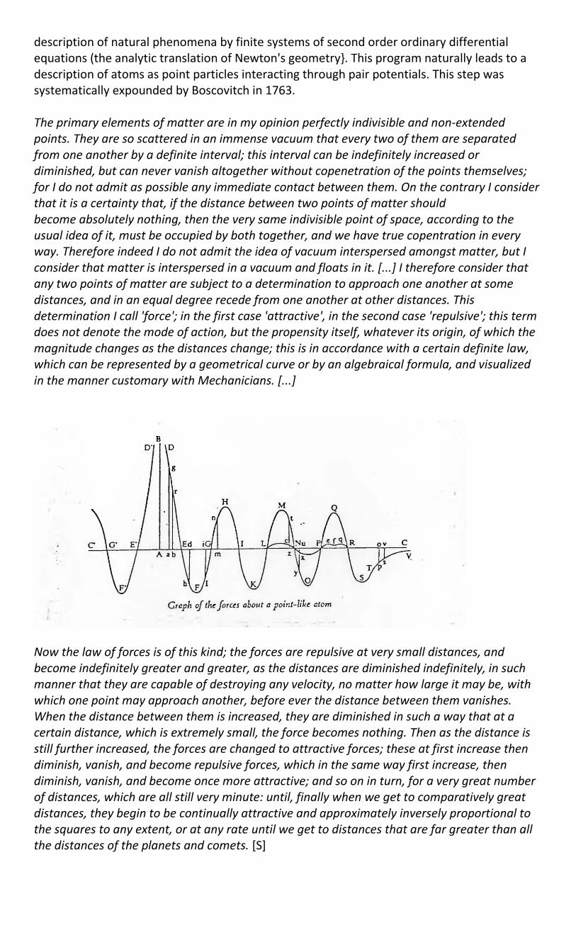
description of natural phenomena by finite systems of second order ordinary differential equations (the analytic translation of Newton's geometry}. This program naturally leads to a description of atoms as point particles interacting through pair potentials. This step was systematically expounded by Boscovitch in 1763. The primary elements of matter are in my opinion perfectly indivisible and non-extended points. They are so scattered in an immense vacuum that every two of them are separated from one another by a definite interval; this interval can be indefinitely increased or diminished, but can never vanish altogether without copenetration of the points themselves; for I do not admit as possible any immediate contact between them. On the contrary I consider that it is a certainty that, if the distance between two points of matter should become absolutely nothing, then the very same indivisible point of space, according to the usual idea of it, must be occupied by both together, and we have true copentration in every way. Therefore indeed I do not admit the idea of vacuum interspersed amongst matter, but I consider that matter is interspersed in a vacuum and floats in it. [...] I therefore consider that any two points of matter are subject to a determination to approach one another at some distances, and in an equal degree recede from one another at other distances. This determination I call 'force'; in the first case 'attractive', in the second case 'repulsive'; this term does not denote the mode of action, but the propensity itself, whatever its origin, of which the magnitude changes as the distances change; this is in accordance with a certain definite law, which can be represented by a geometrical curve or by an algebraical formula, and visualized in the manner customary with Mechanicians. [...]

Now the law of forces is of this kind; the forces are repulsive at very small distances, and become indefinitely greater and greater, as the distances are diminished indefinitely, in such manner that they are capable of destroying any velocity, no matter how large it may be, with which one point may approach another, before ever the distance between them vanishes. When the distance between them is increased, they are diminished in such a way that at a certain distance, which is extremely small, the force becomes nothing. Then as the distance is still further increased, the forces are changed to attractive forces; these at first increase then diminish, vanish, and become repulsive forces, which in the same way first increase, then diminish, vanish, and become once more attractive; and so on in turn, for a very great number of distances, which are all still very minute: until, finally when we get to comparatively great distances, they begin to be continually attractive and approximately inversely proportional to the squares to any extent, or at any rate until we get to distances that are far greater than all the distances of the planets and comets. [S]

Interestingly enough, this natural outcome of the methods and view point of the Principia were definitely not Newton's own view of an intellectually satisfying "ultimate" theory. Newton wrote the following in a letter to Bentley. It is inconceivable, that inanimate brute Matter should, without the Mediation of something else, which is not material, operate upon, and affect other Matter without mutual Contact, as it must be, if Gravitation in the Sense of Epicurus, be essential and inherent in it. And this is one reason why I desired you would not ascribe innate Gravity to me. That Gravity should be innate, inherent and essential to Matter, so that one Body may act upon another at a distance thro' a Vacuum, without the Mediation of anything else, by and through which their Action and Force may be conveyed from one to another, is to me so great an absurdity, that I believe no man who has in philosophical matters a competent faculty of thinking, can ever fall into it. Gravity must be caused by an agent acting constantly according to certain laws; but whether this agent be material or immaterial, I have left to the consideration, of my readers. [S] Boscovitch's theory has many of the same attractions as Plato's theory of geometrical atomism. It is the simplest interesting atomic model within classical mechanics. It was further investigated by Kelvin in the nineteenth century, and, along with its quantum mechanical analog, has been intensely investigated in this century. Kelvin also investigated a very different atomic model which was inspired by Helmholtz's theory of vortices and his own experiments with smoke rings. The mathematics is now that of partial as opposed to ordinary differential equations. This mathematics was developed during the eighteenth century by Euler and others in their attempts to extend Newton's particle mechanics to continuum mechanics. Kelvin worked very hard trying to develop this theory. For example, he computed the vibrational properties of such rings hoping to obtain a theoretical understanding of the spectral lines of atoms that had then been recently discovered. He and Tait also investigated-knot theory and related topics in topology in the hope of founding the ultimate theory. What Kelvin lacked was, mainly, the quantum mechanical algorithm for computing probabilities. Many of his geometric ideas have resurfaced recently in quantum mechanical guise. During the nineteenth century atoms began to be taken much more seriously. Dalton introduced them into chemistry around 1802 and by the middle of the century an essentially modern perspective had been attained. Kelvin had even estimated the size of atoms on the basis of phenomena such as Newton's rings and capillary action. But, though they were constantly appealed to as an explanatory aid, no clear conception of atoms was attained in the nineteenth century.

§2.2. Kinetic Theory. In the second half of the nineteenth century atomic theory entered a new stage with the development of kinetic theory by Clausius, Maxwell and Boltzmann. The exact solution of an N-body problem for large N is certainly not feasible. So, instead, Maxwell introduced the idea of computing certain distribution functions of the system, such as the velocity distribution function f(v,t). For a homogeneous gas in equilibrium, Maxwell was led to the now famous Maxwell distribution f(v)=Ae^(-B|v|2) . Boltzmann extended Maxwell's work by considering the non-equilibrium situation. He derived an integro-differential equation-the Boltzmann equation-for f(v,t) and showed that the Maxwell distribution was its only stationary solution. Furthermore, he introduced the H-integral H(t) = ∫f(v,t) ln f(v,t)dv and showed that if f satisfies the Boltzmann equation, then dH/dt≤ 0 and equals zero only for the Maxwell distribution. Thus, as time goes on the velocity distribution function must go asymptotically to the Maxwell distribution. Boltzmann related H to thermodynamical entropy and considered his H-theorem dH/dt≤ 0 as a microscopic derivation of the second law of thermodynamics. There were (are) a

number of conceptual problems surrounding the Maxwell-Boltzmann theory. As pointed out by Kelvin, Loschmidt, and Zermelo, the microscopic models that the theory was believed to rest upon were time reversible and satisfied Poincare recurrence (a bounded (Hamiltonian) dynamical system will almost surely return arbitrarily close to any initial configuration). Thus, equilibrium will never be attained and H must increase and decrease. If nothing else, these criticisms showed that the "derivations" given by Maxwell and Boltzmann were suspect. Boltzmann responded to Zermelo's criticism as if the situation were really quite simple and he had simply been misunderstood. He accepted the existence of Poincare cycles, but pointed out that they would take so long as to be essentially unobservable. He was thus led to take a "statistical" view of the second law of thermodynamics and to view the Maxwell-Boltzmann theory as merely an approximation valid for large N and relatively small t. Zermelo, in rebuttal, pointed out that while Boltzmann's new viewpoint was certainly conceivable, it was at that time (and still is) only a conjecture, since it was not backed up by hard estimates giving the precise relationship between the exact micro-model and the approximate Maxwell-Boltzmann theory. In any case, the Boltzmann equation can be used as a starting point for the derivation of the transport properties of matter (such as the coefficients in the Navier-Stokes equation of hydrodynamics). Such derivations form the main goal of kinetic theory as envisioned by Maxwell and Boltzmann, and were systematically and successfully developed in the twentieth century by Hilbert, Chapman, Enskog and others. One dramatic success of this later work was the prediction of thermal diffusion. One of the most striking early successes of Maxwell's theory was his theoretical prediction and subsequent empirical verification of the seemingly counter-intuitive fact that the viscosity of a gas is independent of its density. This prediction convinced most physicists to take the kinetic theory seriously. Still, there was uncertainty, and even skepticism, concerning the actual existence of atoms until Einstein's theoretical work on Brownian motion, which analyzed the fluctuations a large particle would undergo due to atomic impacts, was empirically verified by Perrin. By about 1910 the existence of atoms became as unquestioned by physicists as the existence of trees. The Boltzmann equation was meant to describe a dilute gas and only binary collisions were taken into account in its 'derivation'. Attempts to incorporate multiple collisions have run into divergence problems. Even for the Boltzmann equation itself, most work on obtaining approximate solutions (e.g., that of Chapman and Enskog) do not include the hard estimates that would be necessary for full justification of the results claimed. Thus, there is still much work to be done before the Maxwell-Boltzmann program can be said to have truly attained climax status.

§2.3. Statistical Mechanics. While the Maxwell-Boltzmann program was empirically successful, the criticisms of it by Zermelo and others showed that some deeper perspective was necessary. The use of the velocity distribution function is a case of using continuous models even when one believes that the underlying structure is really discrete (see, for comparison, the case studies of the structure of galaxies and of slime mold amoeba in [L-S, Ch. 1]). In almost all cases where such models are used, the precise relationship between the continuum model and the underlying discrete model is quite fuzzy. Most 'derivations' of continuous models from discrete models are really merely plausibility arguments for the continuous model. The continuous model's success or failure is judged more by its simplicity and empirical accuracy than by the rigor of its derivations. But, if such a theory is found to be very successful, it then presents a challenge

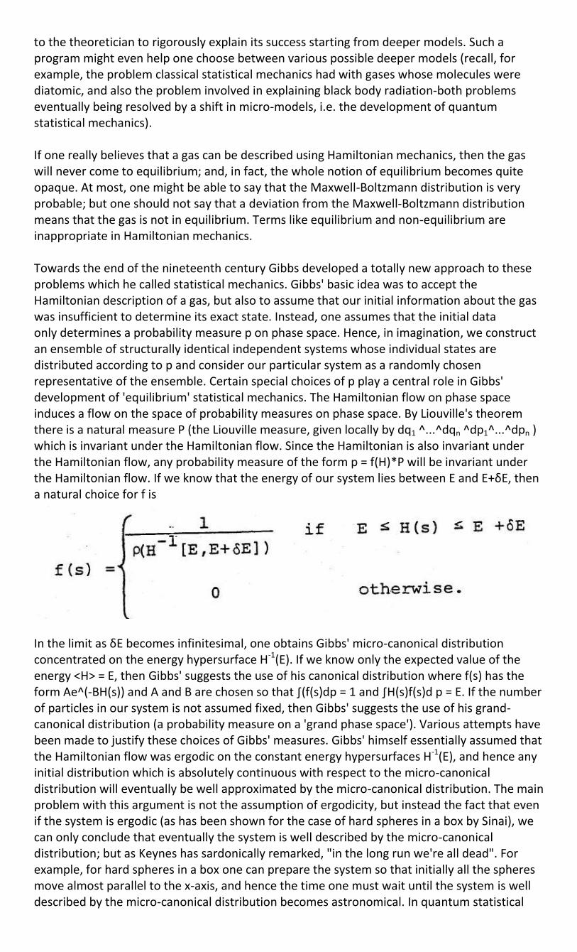
to the theoretician to rigorously explain its success starting from deeper models. Such a program might even help one choose between various possible deeper models (recall, for example, the problem classical statistical mechanics had with gases whose molecules were diatomic, and also the problem involved in explaining black body radiation-both problems eventually being resolved by a shift in micro-models, i.e. the development of quantum statistical mechanics). If one really believes that a gas can be described using Hamiltonian mechanics, then the gas will never come to equilibrium; and, in fact, the whole notion of equilibrium becomes quite opaque. At most, one might be able to say that the Maxwell-Boltzmann distribution is very probable; but one should not say that a deviation from the Maxwell-Boltzmann distribution means that the gas is not in equilibrium. Terms like equilibrium and non-equilibrium are inappropriate in Hamiltonian mechanics. Towards the end of the nineteenth century Gibbs developed a totally new approach to these problems which he called statistical mechanics. Gibbs' basic idea was to accept the Hamiltonian description of a gas, but also to assume that our initial information about the gas was insufficient to determine its exact state. Instead, one assumes that the initial data only determines a probability measure p on phase space. Hence, in imagination, we construct an ensemble of structurally identical independent systems whose individual states are distributed according to p and consider our particular system as a randomly chosen representative of the ensemble. Certain special choices of p play a central role in Gibbs' development of 'equilibrium' statistical mechanics. The Hamiltonian flow on phase space induces a flow on the space of probability measures on phase space. By Liouville's theorem there is a natural measure P (the Liouville measure, given locally by dq1 ^...^dqn ^dp1^...^dpn ) which is invariant under the Hamiltonian flow. Since the Hamiltonian is also invariant under the Hamiltonian flow, any probability measure of the form p = f(H)*P will be invariant under the Hamiltonian flow. If we know that the energy of our system lies between E and E+δE, then a natural choice for f is

In the limit as δE becomes infinitesimal, one obtains Gibbs' micro-canonical distribution concentrated on the energy hypersurface H-1(E). If we know only the expected value of the energy <H> = E, then Gibbs' suggests the use of his canonical distribution where f(s) has the form Ae^(-BH(s)) and A and B are chosen so that ∫(f(s)dp = 1 and ∫H(s)f(s)d p = E. If the number of particles in our system is not assumed fixed, then Gibbs' suggests the use of his grand-canonical distribution (a probability measure on a 'grand phase space'). Various attempts have been made to justify these choices of Gibbs' measures. Gibbs' himself essentially assumed that the Hamiltonian flow was ergodic on the constant energy hypersurfaces H-1(E), and hence any initial distribution which is absolutely continuous with respect to the micro-canonical distribution will eventually be well approximated by the micro-canonical distribution. The main problem with this argument is not the assumption of ergodicity, but instead the fact that even if the system is ergodic (as has been shown for the case of hard spheres in a box by Sinai), we can only conclude that eventually the system is well described by the micro-canonical distribution; but as Keynes has sardonically remarked, "in the long run we're all dead". For example, for hard spheres in a box one can prepare the system so that initially all the spheres move almost parallel to the x-axis, and hence the time one must wait until the system is well described by the micro-canonical distribution becomes astronomical. In quantum statistical

mechanics the situation is even worse in that the appropriate ergodic theorems don't even hold for many models of physical interest. So, instead of trying to justify the use of the Gibbs' measures via ergodic theorems and hard estimates, one can simply recognize their use as a basic postulate concerning the manner in which the system was prepared. Gibbs' variational theorems showing that his canonical distributions minimized a certain integral (which would today be called the information integral) subject to appropriate constraints could be interpreted as a step in this direction. Gibbs also provided arguments which show that if a large system is to be described by the micro-canonical distribution, then a small part of it will often be well described by the canonical or grand-canonical distributions. Applying this argument to a particular particle in a large system yields a 'derivation' of the Maxwell-Boltzmann distribution. A different derivation of the Maxwell-Boltzmann distribution comes by showing that for an ensemble described by one of Gibbs' canoncial distributions an overwhelmingly large proportion of the systems in the ensemble have velocity distributions which are well approximated by the Maxwell-Boltzmann distribution. In Gibbs' approach to statistical mechanics the reasons for using probability arguments are that we are ignorant of the precise initial state of the system and/or we don't want to or can't carry out precise calculations of the Hamiltonian flow. Another point of view is suggested by quantum mechanics. An ensemble of systems of fixed energy E would be described in quantum mechanics by the eigenfunction FE of the Hamiltonian H (we are assuming that E is a non-degenerate eigenvlaue). In the standard interpretation of quantum mechanics, FE determines a priori probability distributions for the results of measurements on the system; the use of probability here being considered intrinsic and not due to any ignorance on the part of the observer. In particular, FE is assumed to be applicable not only to the ensemble but also to each individual system in the ensemble. For example, a container of gas could be looked at with a position microscope which would yield a collection of points in R. FE determines a probability distribution on the set of such collections of points. The "atoms" are not assumed to be somewhere before the measurement; an atomic model in quantum mechanics makes an assumption of certain modes of perceiving and not that of the existence of certain small objects (see [E-1] for a detailed discussion of these issues). The classical analog of FE is the micro-canonical distribution PE (assuming that the Hamiltonian determines an ergodic flow on the hypersurface H = E). This suggests taking a quantum mechanical viewpoint even when the "logic" of the system is Boolean. We are suggesting that the microcanonical distribution p may not only be applicable to ensembles of systems but also to individual systems. This viewpoint has several advantages. First of all, it allows us to talk about an individual sample of gas being in equilibrium; namely, its state is pE, which doesn't change in time. Furthermore, we not only get equilibrium, but also fluctuations whose probability can be computed using pE. Moreover, in the nonequilibrium situation, it allows us to consider much more general possibilities for the dynamics of the system. For example, instead of assuming that the dynamics is generated by an underlying Hamiltonian flow, one can instead assume that one only has the semi-group R acting on the probability measures on phase space. Thus, one might choose an evolution which really does evolve towards equilibrium. This would be analogous to taking a master equation as fundamental and not considering it as an approximation to underlying Liouville equations. This viewpoint also suggests the possibility of the compatibility of statistical mechanics with the Boltzmann equation interpreted in a new way. In this view, f would not represent the evolution of the velocity distribution function for a single system (and hence the original derivation of the Boltzmann equation for f would be invalidated); but, instead, it would represent a distribution near which, with overwhelming probability, the actual measured distribution would be found. This point of view would be particularly important in quantum mechanics because in the usual description of particles via the Schrodinger equation the 'particles' don't have trajectories (a similar point could also be

made about the usual Hamiltonian formulation of Mechanics wherein there are no trajectory questions). This relationship has been worked out in detail for some simplified models such as the Kac ring model (see [T, p. 23]). This viewpoint is strikingly different from the original viewpoint of Maxwell and Boltzmann.

§2.4 Thermodynamical Analogies and other Applications of Statistical Mechanics. One of the main goals of statistical mechanics is the derivation and explication of macroscopic phenomena starting from microscopic models; three paradigmatic cases being the usual explanations of pressure, temperature, and Brownian motion. Let us consider these paradigmatic cases more carefully. The macroscopic phenomena of pressure exerted by a gas on its container walls is usually explained as due to the impacts of the gas molecules on those walls. In fact, quite simple models even allow one to derive such quantitative relations as Boyle's Law. Brownian motion is usually explained as due to fluctuations in the impacts of the fluid molecules on the larger suspended particles. From this picture and statistical mechanics, Einstein was able to derive quantitative relations governing Brownian motion. Temperature is also usually explained as due to the average motion of the molecules. These standard explanations, besides being quantitatively accurate, are also intellectually very satisfying in that they fulfill our normal everyday criteria for a satisfying, causal, mechanistic explanation. Unfortunately, these satisfying accounts of macroscopic phenomena unravel when one passes from classical mechanical models of atoms and molecules over to quantum mechanical models. This is because in the usual Schrodinger model of atoms, one has position observables, but no trajectory observables, i.e. the atoms have no paths. So, immediately our explanations and calculations which were based upon the notion of impacts of molecules dissolve. A compensation is that one can now rigorously derive the Maxwell-Boltzmann distribution for the energy distribution of molecules of a gas in equilibrium (note, this is an energy distribution and not a velocity distribution because in the usual Schrodinger model, molecules have momentum and energy observables but no velocity observables). One also gains an understanding of why the specific heats of gases whose molecules are diatomic behave as if their molecules have only five instead of six degrees of freedom. There are these, and many other similar compensations for our lost mechanical explanations; but in order to obtain these compensations we must first find some connection between our microscopic and macroscopic models. This connection is obtained by defining certain functions of our statistical mechanical model which are to be identified with certain functions occurring in thermodynamics. The most important of these functions are the thermodynamical potentials, ψ the Helmholtz free energy, and φ, the Gibbs potential. In thermodynamics these functions are defined by ψ=U - TS and φ=U - TS + PV and one proves the following theorem (see [T] ) THEOREM: 1. For a mechanically isolated system at constant temperature, ψ never increases. The thermal equilibrium state for such a system is then the state of minimum ψ. 2. For a system at constant pressure and temperature, φ never increases. The equilibrium state for such a system is then the state of minimum φ. If ψ is viewed as a function of V and T by eliminating its explicit dependence upon P through an equation of state relating P, V and T, then one can derive various Maxwell relations such as P = - (d ψ /dV)T and S=-(d ψ /dT)V . Conversely, if ψ is given as a function of V and T, then the Maxwell relations can be converted into definitions and equations of state. One thus sees that all thermodynamic relations are obtainable from an explicit knowledge of ψ as a function of V and T. In thermodynamics the explicit form for ψ appropriate to describe some physical system must be taken as a fundamental assumption. (Particular assumptions being, of course, motivated by the hope of obtaining a close analogy between the behavior of the physical system and of the model.) One of the main goals of statistical mechanics is to derive explicit

forms for ψ starting from its deeper assumptions. But one must then not forget that in statistical mechanics concepts such as pressure are being defined by the Maxwell relations, and no longer carry such colorful images as being do to impacts. This point will become clearer as we examine some explicit models.

§ 2.5 The Ising Model Since its introduction in the 1920's by Lenz and Ising, The Ising Model has become one of the most important models in modern physics because it is the simplest non-trivial model of cooperative phenomena. The model consists of a finite collection σ = {σi l 1<= i<=N} of compatible two-valued observables σi, where the index i is viewed to vary over a square lattice of side L (N = Ld , where d is the dimension of the lattice). If the values of σi are denoted by -1 and +1, then a configuration of σ determines a point in C= {-1, + 1}N , and a joint probability measure u for the σi’s determines a probability measure on C. From the state u one can compute various means such as < σi >, < σi σj>, etc. These means can be empirically determined (at least approximately) by choosing a large ensemble of identically prepared systems (i.e., each is in a state determined by the a priori probability distribution u) and computing the average over the ensemble of the values empirically obtained for σi, σiσj, etc. (of course, the actual means < σi >, < σi σj> would only be obtained in this way with probability one in the limit of an infinitely large ensemble.) In this way we obtain new observables < σi >, <σiσj>, etc., which we shall call second order observables. If we have a family of states u depending upon a parameter a varying, say, in Rn then we would naturally be interested in the analytic properties < σi >a, < σiσj>a, etc., as a function of the parameter a. In this way we could introduce new (third order) observables

etc. In statistical mechanics particular attention is focused upon the probability measures first introduced by Gibbs. In the context of The Ising Model, the Gibbs distributions are defined as follows: a) the micro-canonical distribution uM corresponding to a fixed total energy E associates a probability

each σ such that H(σ) = E, where H is the Hamiltonian of the system (e.g., in the simplest case taken to be

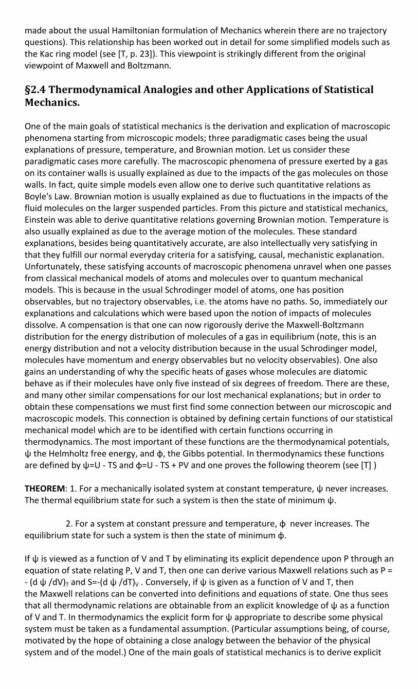
; b) the canonical distribution corresponding to a fixed mean energy <H> = E is given by

, where β is chosen so that

(Note, that since we want uc

β to be a probability measure, it is necessary that β be an extended real number, but nothing in the model requires that β > 0. This suggests that one should look for phenomena for which it would be appropriate to ascribe a 'negative' temperature and develop the appropriate thermodynamics.) c) The grand canonical distribution corresponding to a fixed mean energy <H> = E and a fixed mean number of particles is given by

There are various ways of attempting to motivate these distributions. These distributions can be shown to minimize "information" (equivalently, maximize entropy) subject to their respective constraints. Furthermore, if one assumes that the micro-canonical distribution applies to a large system, central limit type arguments lead to the canonical or grand canonical distributions for the description of certain small subsystems. But the way we favor most of motivating these distributions is to simply recognize the use of these Gibbs' measures as a basic postulate concerning the manner of preparation of the system. Alternatively, from the point of view of pure probability theory, these Gibbs' measures define a simple model of a family of random variables which are strongly dependent upon their neighbors. To the Gibbs' canonical and grand canonical distributions one associates the partition functions

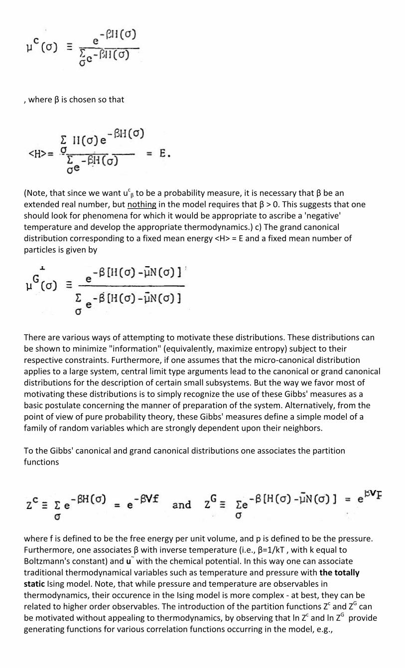
where f is defined to be the free energy per unit volume, and p is defined to be the pressure. Furthermore, one associates β with inverse temperature (i.e., β=1/kT , with k equal to Boltzmann's constant) and u~ with the chemical potential. In this way one can associate traditional thermodynamical variables such as temperature and pressure with the totally static Ising model. Note, that while pressure and temperature are observables in thermodynamics, their occurence in the Ising model is more complex - at best, they can be related to higher order observables. The introduction of the partition functions Zc and ZG can be motivated without appealing to thermodynamics, by observing that ln Zc and ln ZG provide generating functions for various correlation functions occurring in the model, e.g.,

,

Obvious extensions of The Ising Model are obtained by considering more general lattices, Hamiltonians, and spin variables (i.e., allowing sigmai to take on values in a range X more general than Z2 , e.g. X = R or S2 ). One can also consider quantum mechanical analogs where not all the sigmai are compatible; in this case one uses Gibbs-von Neumann density matrices such

with its associated partition function

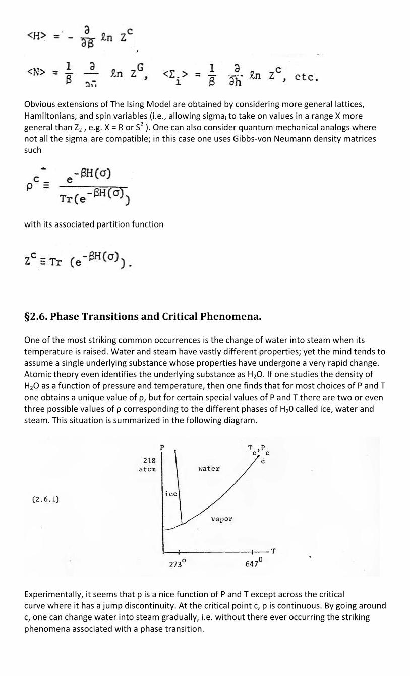
§2.6. Phase Transitions and Critical Phenomena. One of the most striking common occurrences is the change of water into steam when its temperature is raised. Water and steam have vastly different properties; yet the mind tends to assume a single underlying substance whose properties have undergone a very rapid change. Atomic theory even identifies the underlying substance as H2O. If one studies the density of H2O as a function of pressure and temperature, then one finds that for most choices of P and T one obtains a unique value of ρ, but for certain special values of P and T there are two or even three possible values of ρ corresponding to the different phases of H20 called ice, water and steam. This situation is summarized in the following diagram.

Experimentally, it seems that ρ is a nice function of P and T except across the critical curve where it has a jump discontinuity. At the critical point c, ρ is continuous. By going around c, one can change water into steam gradually, i.e. without there ever occurring the striking phenomena associated with a phase transition.

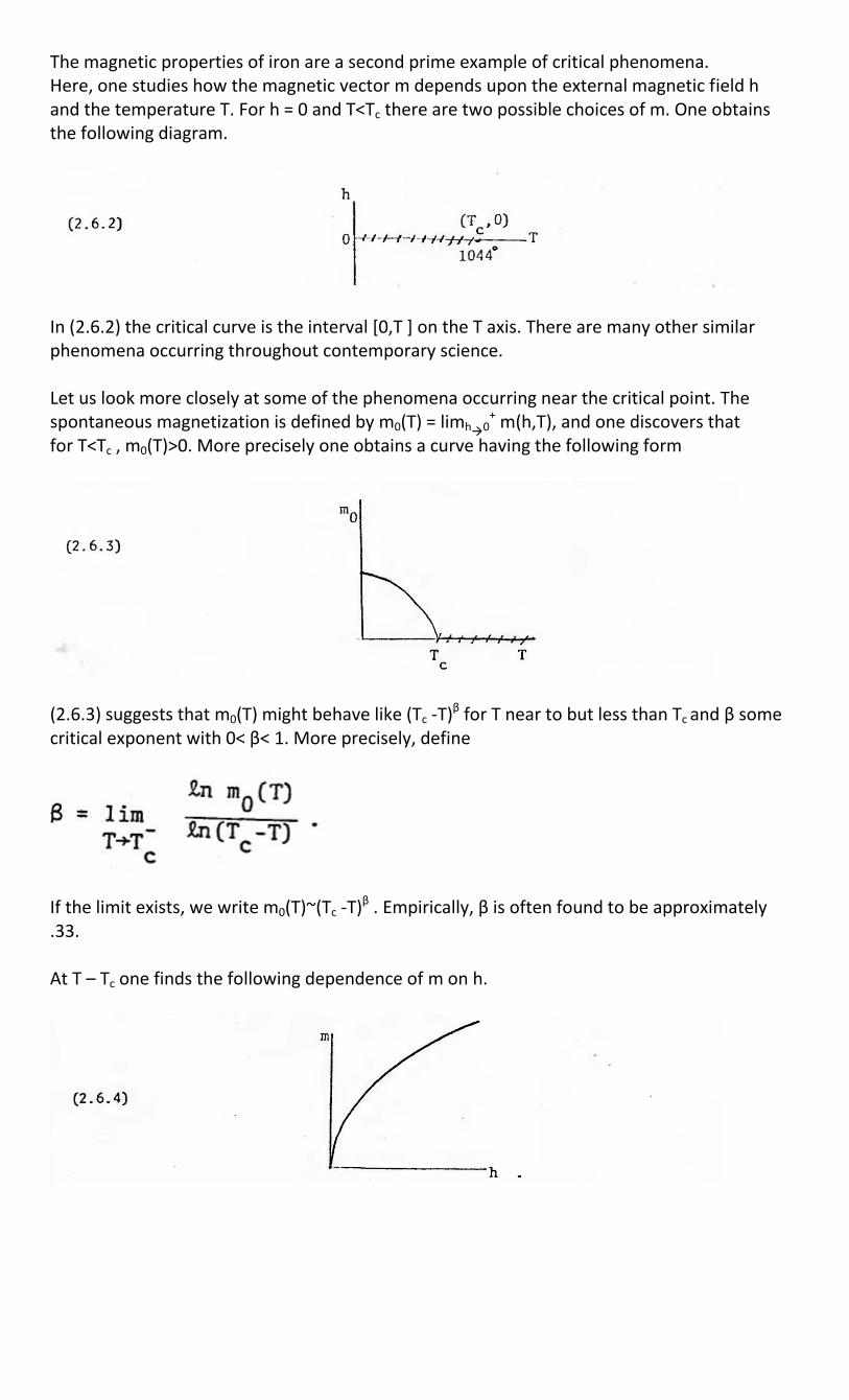
The magnetic properties of iron are a second prime example of critical phenomena. Here, one studies how the magnetic vector m depends upon the external magnetic field h and the temperature T. For h = 0 and T<Tc there are two possible choices of m. One obtains the following diagram.

In (2.6.2) the critical curve is the interval [0,T ] on the T axis. There are many other similar phenomena occurring throughout contemporary science. Let us look more closely at some of the phenomena occurring near the critical point. The spontaneous magnetization is defined by m0(T) = limh

0

+ m(h,T), and one discovers that for T<Tc , m0(T)>0. More precisely one obtains a curve having the following form

(2.6.3) suggests that m0(T) might behave like (Tc -T)β for T near to but less than Tc and β some critical exponent with 0< β< 1. More precisely, define

If the limit exists, we write m0(T)~(Tc -T)β . Empirically, β is often found to be approximately .33. At T – Tc one finds the following dependence of m on h.

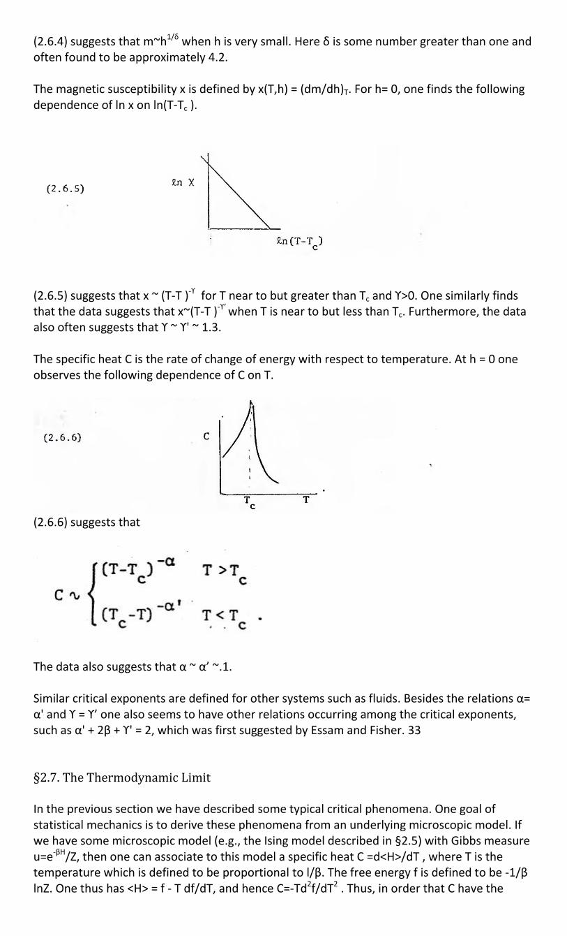
(2.6.4) suggests that m~h1/δ when h is very small. Here δ is some number greater than one and often found to be approximately 4.2. The magnetic susceptibility x is defined by x(T,h) = (dm/dh)T. For h= 0, one finds the following dependence of ln x on ln(T-Tc ).

(2.6.5) suggests that x ~ (T-T )-ϒ for T near to but greater than Tc and ϒ>0. One similarly finds that the data suggests that x~(T-T )-ϒ’ when T is near to but less than Tc. Furthermore, the data also often suggests that ϒ ~ ϒ' ~ 1.3. The specific heat C is the rate of change of energy with respect to temperature. At h = 0 one observes the following dependence of C on T.

(2.6.6) suggests that

The data also suggests that α ~ α’ ~.1. Similar critical exponents are defined for other systems such as fluids. Besides the relations α= α' and ϒ = ϒ’ one also seems to have other relations occurring among the critical exponents, such as α' + 2β + ϒ' = 2, which was first suggested by Essam and Fisher. 33 §2.7. The Thermodynamic Limit In the previous section we have described some typical critical phenomena. One goal of statistical mechanics is to derive these phenomena from an underlying microscopic model. If we have some microscopic model (e.g., the Ising model described in §2.5) with Gibbs measure u=e-βH/Z, then one can associate to this model a specific heat C =d<H>/dT , where T is the temperature which is defined to be proportional to l/β. The free energy f is defined to be -1/β lnZ. One thus has <H> = f - T df/dT, and hence C=-Td2f/dT2 . Thus, in order that C have the

singularity structure at the critical temperature Tc which was described in §2.6, it is necessary that f be a non-analytic function of T at T=Tc . In the case of the Ising model for N spins, one has

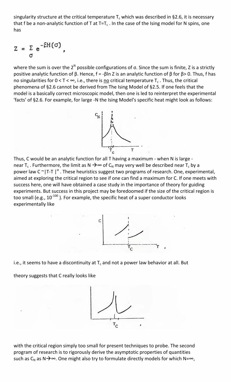
where the sum is over the 2N possible configurations of σ. Since the sum is finite, Z is a strictly positive analytic function of β. Hence, f = -βln Z is an analytic function of β for β> 0. Thus, f has no singularities for 0 < T < ∞, i.e., there is no critical temperature Tc . Thus, the critical phenomena of §2.6 cannot be derived from The Ising Model of §2.5. If one feels that the model is a basically correct microscopic model, then one is led to reinterpret the experimental 'facts' of §2.6. For example, for large -N the Ising Model's specific heat might look as follows:

Thus, C would be an analytic function for all T having a maximum - when N is large - near Tc . Furthermore, the limit as N ∞ of CN may very well be described near Tc by a power law C ~|T-T |α . These heuristics suggest two programs of research. One, experimental, aimed at exploring the critical region to see if one can find a maximum for C. If one meets with success here, one will have obtained a case study in the importance of theory for guiding experiments. But success in this project may be foredoomed if the size of the critical region is too small (e.g., 10-100 ). For example, the specific heat of a super conductor looks experimentally like

i.e., it seems to have a discontinuity at Tc and not a power law behavior at all. But theory suggests that C really looks like

with the critical region simply too small for present techniques to probe. The second program of research is to rigorously derive the asymptotic properties of quantities such as CN as N∞. One might also try to formulate directly models for which N=∞,

and to derive their thermodynamic properties.

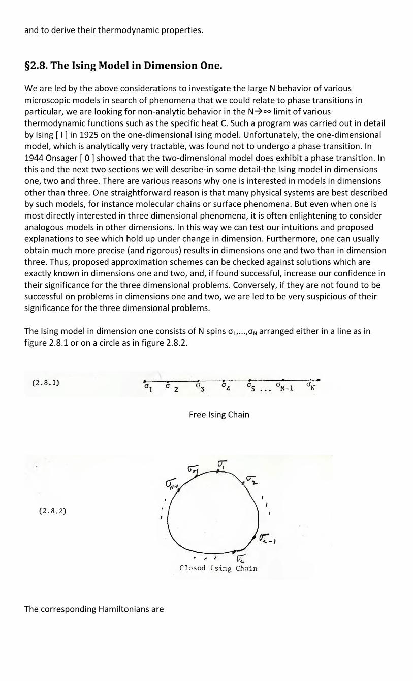
§2.8. The Ising Model in Dimension One. We are led by the above considerations to investigate the large N behavior of various microscopic models in search of phenomena that we could relate to phase transitions in particular, we are looking for non-analytic behavior in the N∞ limit of various thermodynamic functions such as the specific heat C. Such a program was carried out in detail by Ising [ I ] in 1925 on the one-dimensional Ising model. Unfortunately, the one-dimensional model, which is analytically very tractable, was found not to undergo a phase transition. In 1944 Onsager [ 0 ] showed that the two-dimensional model does exhibit a phase transition. In this and the next two sections we will describe-in some detail-the Ising model in dimensions one, two and three. There are various reasons why one is interested in models in dimensions other than three. One straightforward reason is that many physical systems are best described by such models, for instance molecular chains or surface phenomena. But even when one is most directly interested in three dimensional phenomena, it is often enlightening to consider analogous models in other dimensions. In this way we can test our intuitions and proposed explanations to see which hold up under change in dimension. Furthermore, one can usually obtain much more precise (and rigorous) results in dimensions one and two than in dimension three. Thus, proposed approximation schemes can be checked against solutions which are exactly known in dimensions one and two, and, if found successful, increase our confidence in their significance for the three dimensional problems. Conversely, if they are not found to be successful on problems in dimensions one and two, we are led to be very suspicious of their significance for the three dimensional problems. The Ising model in dimension one consists of N spins σ1,...,σN arranged either in a line as in figure 2.8.1 or on a circle as in figure 2.8.2.

Free Ising Chain

The corresponding Hamiltonians are

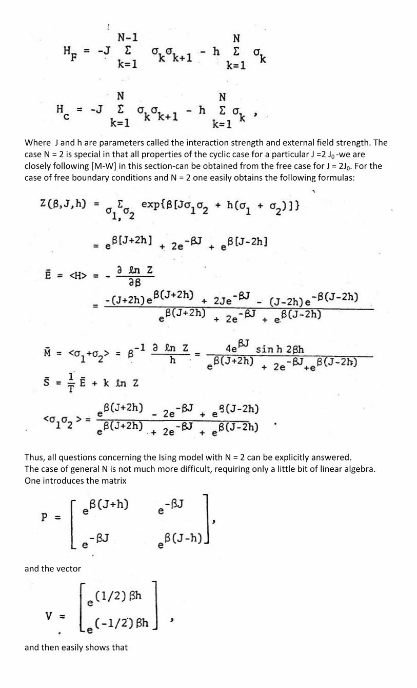
Where J and h are parameters called the interaction strength and external field strength. The case N = 2 is special in that all properties of the cyclic case for a particular J =2 J0 -we are closely following [M-W] in this section-can be obtained from the free case for J = 2J0. For the case of free boundary conditions and N = 2 one easily obtains the following formulas:

Thus, all questions concerning the Ising model with N = 2 can be explicitly answered. The case of general N is not much more difficult, requiring only a little bit of linear algebra. One introduces the matrix

and the vector

and then easily shows that

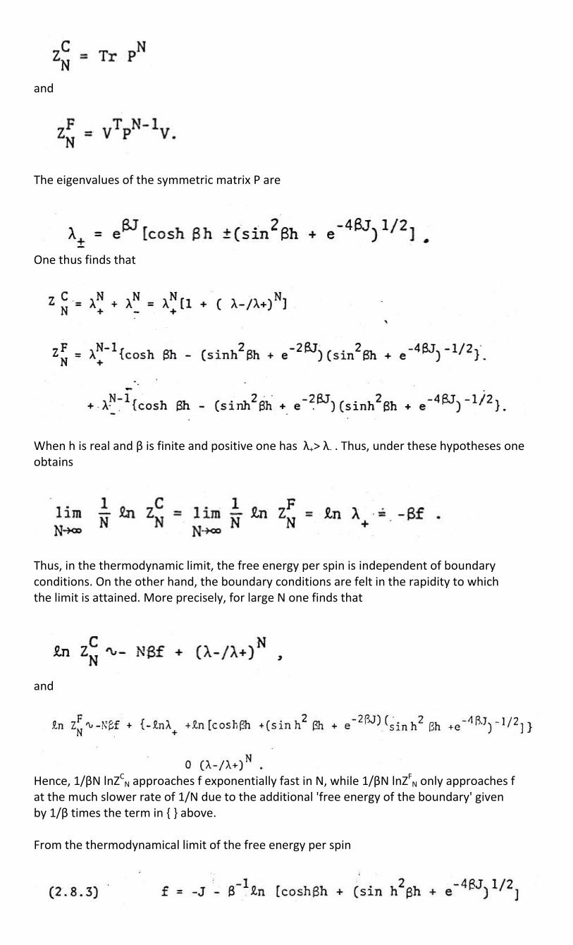
and

The eigenvalues of the symmetric matrix P are

One thus finds that

When h is real and β is finite and positive one has λ+> λ- . Thus, under these hypotheses one obtains

Thus, in the thermodynamic limit, the free energy per spin is independent of boundary conditions. On the other hand, the boundary conditions are felt in the rapidity to which the limit is attained. More precisely, for large N one finds that

and

Hence, 1/βN lnZC

N approaches f exponentially fast in N, while 1/βN lnZFN only approaches f

at the much slower rate of 1/N due to the additional 'free energy of the boundary' given by 1/β times the term in { } above. From the thermodynamical limit of the free energy per spin

we can obtain the other thermodynamic quantities such as the specific heat

and the magnetization

Below are some graphs (from [M-W]) for the ferromagnetic case J/k = 1

From the explicit form of f (2.8.3) we see that f is an analytic function of its parameters for all real J and h and all P >0. Thus, the Ising model in dimension one does not undergo a phase transition (in the sense of non-analytic points of f for 'physical' values of its parameters). One can go further and compute the various spin-spin correlation functions. For <σiσj>

FN one

obtains a mess that depends explicitly on i and j and not only on i-j. Thus, various thermodynamic limits can be taken of this quantity. If we hold i and j fixed and let N∞ we obtain the asymptotic form of the correlation of two spins which are a finite distance from the

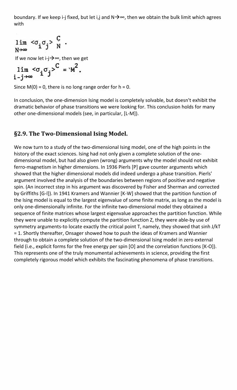
boundary. If we keep i-j fixed, but let i,j and N∞, then we obtain the bulk limit which agrees with

If we now let i-j∞, then we get

Since M(0) = 0, there is no long range order for h = 0. In conclusion, the one-dimension Ising model is completely solvable, but doesn't exhibit the dramatic behavior of phase transitions we were looking for. This conclusion holds for many other one-dimensional models (see, in particular, [L-M]).

§2.9. The Two-Dimensional Ising Model. We now turn to a study of the two-dimensional Ising model, one of the high points in the history of the exact sciences. Ising had not only given a complete solution of the one-dimensional model, but had also given (wrong) arguments why the model should not exhibit ferro-magnetism in higher dimensions. In 1936 Pierls [P] gave counter arguments which showed that the higher dimensional models did indeed undergo a phase transition. Pierls' argument involved the analysis of the boundaries between regions of positive and negative spin. (An incorrect step in his argument was discovered by Fisher and Sherman and corrected by Griffiths [G-l]). In 1941 Kramers and Wannier [K-W] showed that the partition function of the Ising model is equal to the largest eigenvalue of some finite matrix, as long as the model is only one-dimensionally infinite. For the infinite two-dimensional model they obtained a sequence of finite matrices whose largest eigenvalue approaches the partition function. While they were unable to explicitly compute the partition function Z, they were able-by use of symmetry arguments-to locate exactly the critical point T, namely, they showed that sinh J/kT = 1. Shortly thereafter, Onsager showed how to push the ideas of Kramers and Wannier through to obtain a complete solution of the two-dimensional Ising model in zero external field (i.e., explicit forms for the free energy per spin [O] and the correlation functions [K-O]). This represents one of the truly monumental achievements in science, providing the first completely rigorous model which exhibits the fascinating phenomena of phase transitions.

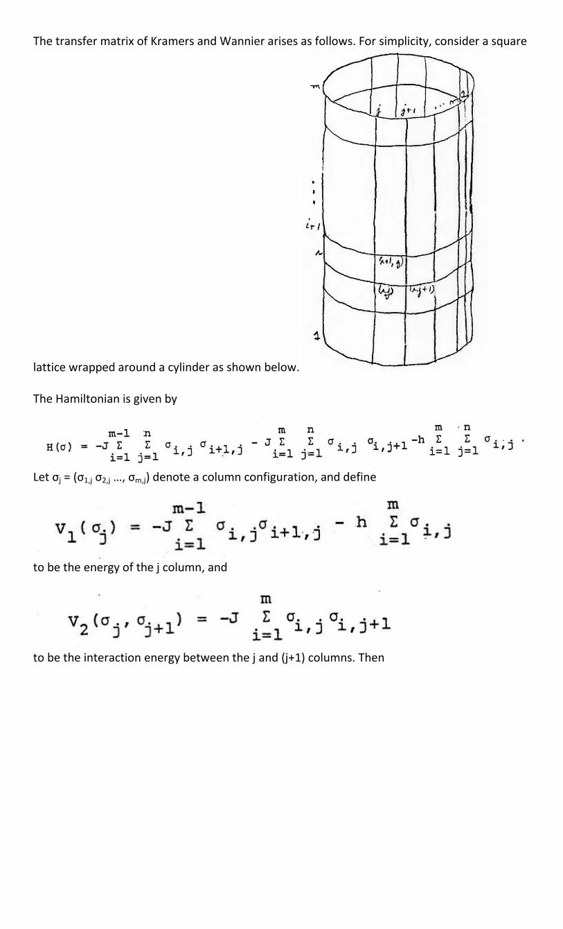
The transfer matrix of Kramers and Wannier arises as follows. For simplicity, consider a square

lattice wrapped around a cylinder as shown below. The Hamiltonian is given by

Let σj = (σ1,j σ2,j …, σm,j) denote a column configuration, and define

to be the energy of the j column, and

to be the interaction energy between the j and (j+1) columns. Then

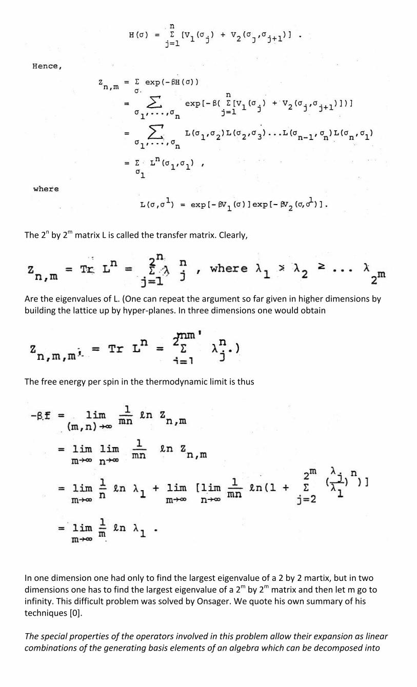
The 2n by 2m matrix L is called the transfer matrix. Clearly,

Are the eigenvalues of L. (One can repeat the argument so far given in higher dimensions by building the lattice up by hyper-planes. In three dimensions one would obtain

The free energy per spin in the thermodynamic limit is thus

In one dimension one had only to find the largest eigenvalue of a 2 by 2 martix, but in two dimensions one has to find the largest eigenvalue of a 2m by 2m matrix and then let m go to infinity. This difficult problem was solved by Onsager. We quote his own summary of his techniques [0]. The special properties of the operators involved in this problem allow their expansion as linear combinations of the generating basis elements of an algebra which can be decomposed into

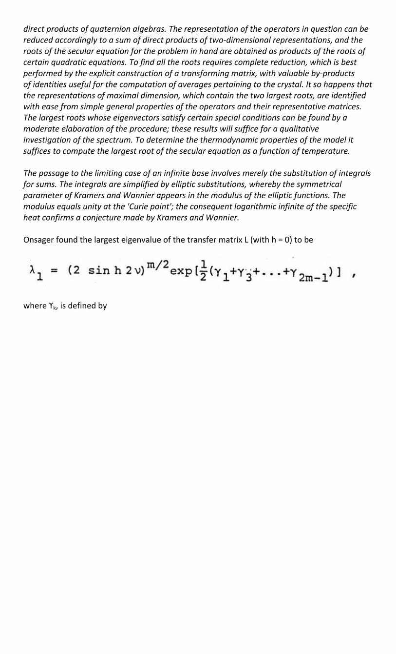
direct products of quaternion algebras. The representation of the operators in question can be reduced accordingly to a sum of direct products of two-dimensional representations, and the roots of the secular equation for the problem in hand are obtained as products of the roots of certain quadratic equations. To find all the roots requires complete reduction, which is best performed by the explicit construction of a transforming matrix, with valuable by-products of identities useful for the computation of averages pertaining to the crystal. It so happens that the representations of maximal dimension, which contain the two largest roots, are identified with ease from simple general properties of the operators and their representative matrices. The largest roots whose eigenvectors satisfy certain special conditions can be found by a moderate elaboration of the procedure; these results will suffice for a qualitative investigation of the spectrum. To determine the thermodynamic properties of the model it suffices to compute the largest root of the secular equation as a function of temperature. The passage to the limiting case of an infinite base involves merely the substitution of integrals for sums. The integrals are simplified by elliptic substitutions, whereby the symmetrical parameter of Kramers and Wannier appears in the modulus of the elliptic functions. The modulus equals unity at the 'Curie point'; the consequent logarithmic infinite of the specific heat confirms a conjecture made by Kramers and Wannier. Onsager found the largest eigenvalue of the transfer matrix L (with h = 0) to be

where ϒk, is defined by

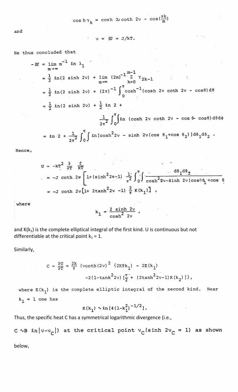
and K(k1) is the complete elliptical integral of the first kind. U is continuous but not differentiable at the critical point k1 = 1. Similarly,

Thus, the specific heat C has a symmetrical logarithmic divergence (i.e.,

below,

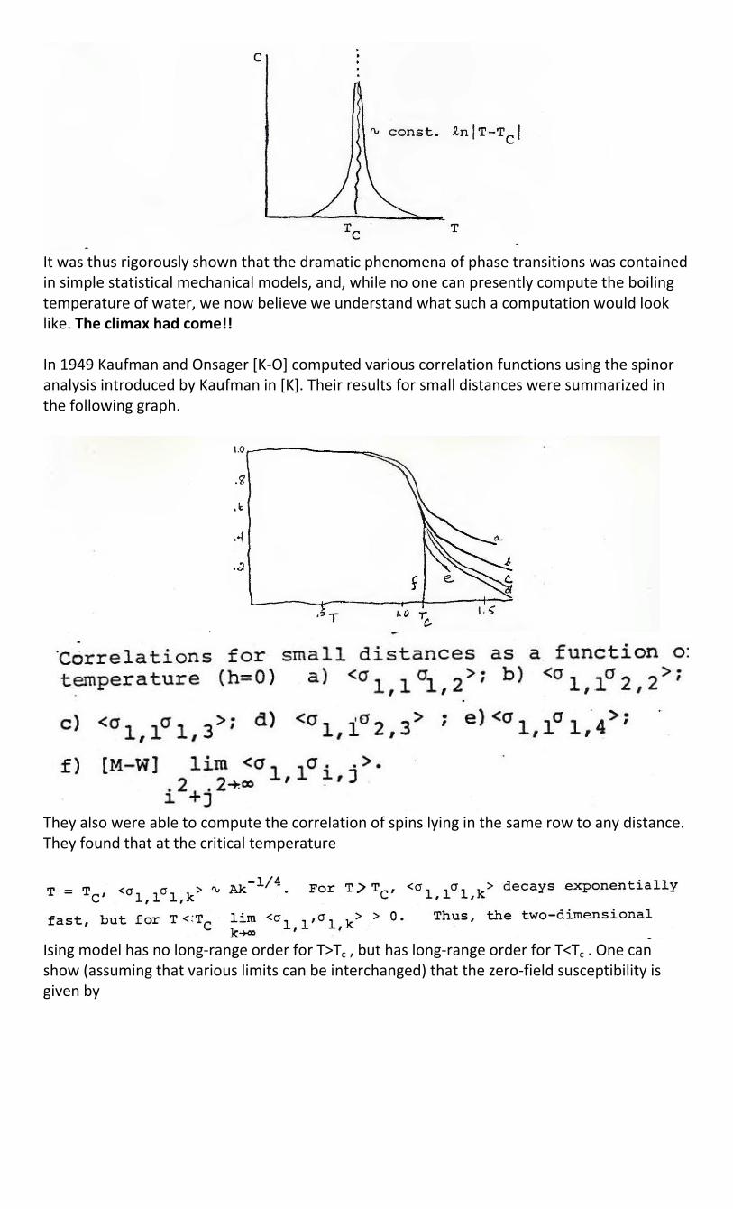
It was thus rigorously shown that the dramatic phenomena of phase transitions was contained in simple statistical mechanical models, and, while no one can presently compute the boiling temperature of water, we now believe we understand what such a computation would look like. The climax had come!! In 1949 Kaufman and Onsager [K-O] computed various correlation functions using the spinor analysis introduced by Kaufman in [K]. Their results for small distances were summarized in the following graph.

They also were able to compute the correlation of spins lying in the same row to any distance. They found that at the critical temperature

Ising model has no long-range order for T>Tc , but has long-range order for T<Tc . One can show (assuming that various limits can be interchanged) that the zero-field susceptibility is given by

These formulas can be verified on the one-dimensional model which can be solved exactly even for h~=0. For the two-dimensional model, no one has been able to explicitly compute the free energy per spin for h~= 0. But one can show [M-W] that the limit

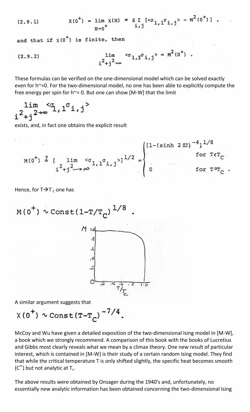
exists, and, in fact one obtains the explicit result

Hence, for TT-

C one has

A similar argument suggests that

McCoy and Wu have given a detailed exposition of the two-dimensional Ising model in [M-W], a book which we strongly recommend. A comparison of this book with the books of Lucretius and Gibbs most clearly reveals what we mean by a climax theory. One new result of particular interest, which is contained in [M-W] is their study of a certain random Ising model. They find that while the critical temperature T is only shifted slightly, the specific heat becomes smooth (C∞) but not analytic at Tc. The above results were obtained by Onsager during the 1940's and, unfortunately, no essentially new analytic information has been obtained concerning the two-dimensional Ising

model since then. The model can be reformulated as a dimer problem, and any dimer problem on a planar lattice can be solved and the solution expressed as a Pfaffian. One can also introduce a quantum field theory formalism in terms of admission and absorption of bonds. These alternative formalisms all yield the same results.

References

[Br-1] S. Brush, History of the Lenz-Ising Model, Rev. Mod. Phys. 39, 883 (1967). [Br-2]_______________, Kinetic Theory, 3 vols., Pergamon Press, Elmsford,N.Y.TT965). [Br-3] _______________, The Kind of Motion we call Heat, 2 vols.,North Holland Pub. Co., New York (1976). [D-G] C. Domb and M. Green, Phase Transitions and Critical Phenomena, 6 vols., Academic Press(1972). [E-1] D. Edwards, The Mathematical Foundations of Quantum Mechanics, http://www.springerlink.com/content/g047367766j30t07/ [E-2] D. Edwards, The Mathematical Foundations of Quantum Field Theory, http://www.springerlink.com/content/m474808n785m3491/

[E-3] D. Edwards, The Structure of Superspace, published in: Studies in Topology, Academic Press, 1975

[E-4] D. Edwards, Atomic Discourse in the Feynman Lectures on Physics, http://www.springerlink.com/content/v60l01k93n272141/

[E-W] D. Edwards and S. Wilcox, Unity, Disunity and Pluralism in Science,

http://arxiv.org/abs/1110.6545

[E-E] P. Ehrenfest and T. Ehrenfest, The Conceptual Foundations of the Statistical Approach in Mechanics, Cornell University Press, Ithaca, N.Y. [G] J. Gibbs, Collected Works, Yale University Press. [G-l] R. Griffiths, Pierls Proof of Spontaneous Magnetization in a two-dimensional Ising Fierromagnetic, Phys. Rev. 136A, 437 (1964). [I] E. Ising, Beitrag zur Theorie des Ferromagnetismus, Z. Physik 31, 253 (1925). [K] B. Kaufman, Crystal Statistics, II. Partition Function Evaluated by Spinor Analysis, Phys. Rev. 76, 1232 (1949). [K-0] _________________ and L. Onsager, Crystal Statistics,III. Short Range Order in a Binary Ising Lattice, Phys. Rev. 76, 1244 (1949). [K-W] H. Kramers and G. Wannier, Statistics of the Two-dimensional Fierromagnet, I and II, Phys. Rev. 60, 252, 263 (1941). [L-Y] T. Lee and C. Yang, Statistical theory of Equations of State and Phase Transitions, I and II, Phys. Rev. 87, 404, 410. (1952).

[L-M] E. Lieb and D. Mattis, Mathematical Physics in One Dimension, Academic Press, New York (1966). [L-Sl C. Lin and L. Segel, Mathematics Applied to Deterministic Problems in the Natural Sciences, McMillan. [M] S. Ma, Modern Theory of Critical Phenomena, W. A. Benjamin, Inc. (1976). [M-Wl B. McCoy and T. Wu, The Two-Dimensional Ising Model, Harvard University Press (1973). [0] L. Onsager, Crystal Statistics, I. A. Two-Dimensional Model with an Order-Disorder Transition, Phys. Rev. 65, 117 (1944). [P] R. Pierls, On Ising's Model of Ferromagnetism, Proc. Cambridge Phil. Soc. 32, 477 (1936). [R] D. Ruelle, Statistical Mechanics: Rigorous Results, W. A. Benjamin, New York (1969). [S] S. Sambursky, Physical Thought from the Pre-Socratics to the Quantum Physicists, PICA Press, New York (1974). [T] C. Thompson, Mathematical Statistical Mechanics, Princeton University Press (1979).