CALPHAD: Computer Coupling of Phase Diagrams and Thermochemistry 33 (2009) 237–243

Contents lists available at ScienceDirect

CALPHAD: Computer Coupling of Phase Diagrams andThermochemistry

journal homepage: www.elsevier.com/locate/calphad

Phase field simulations in miscibility gapsM.H. Braga a,∗, J.C.R.E. Oliveira b, L.F. Malheiros c, J.A. Ferreira da CEMUC, Department of Eng. Physics, FEUP, R. Dr. Roberto Frias s/n, 4200-465 Porto, Portugalb CFP, Department of Eng. Physics, FEUP, R. Dr. Roberto Frias s/n, 4200-465 Porto, Portugalc CEMUC, Department of Metall. and Mat. Eng., FEUP, R. Dr. Roberto Frias s/n, 4200-465 Porto, Portugald LNEG Laboratory, R. da Amieira - Apartado 1089, S. Mamede Infesta, Portugal

a r t i c l e i n f o

Article history:Received 19 May 2008Received in revised form29 September 2008Accepted 6 October 2008Available online 6 November 2008

Keywords:SpinodalPhase field simulationsBi–ZnVycorSol–gel

a b s t r a c t

Using phase field simulations, it is possible to simulate the dynamics and morphology of immiscibleliquids/solids appearing at the miscibility gap of any system. These simulations may also be used todetermine the asymptotic compositions of the fluids for a given Gibbs energy. Even more, it is knownthat different parameters of the excess Gibbs energy of a certain phase may exhibit different asymptoticmorphologies, in spite of the similarity of the associated equilibrium curves. This method can be usedto choose the best excess Gibbs energy’ parameters for the liquid (or solid) phase of a system that willsuffer spinodal decomposition. It can also be important (like in the sol–gel process) to choose the bestcomposition, temperature and time to obtain a certain wanted morphology, just by means of the Gibbsenergy of the respective phase. In thiswork, we have performed phase field simulations of the two liquid’sseparation occurring in the Bi–Zn system, for different temperatures, concentrations and times. We havefound a rich diversity of asymptotic morphologies for different points of the Bi–Zn phase diagram. Twodifferent Gibbs energieswere used to showhow themorphologieswill be affected by different parametersof the excess Gibbs energy.

© 2008 Elsevier Ltd. All rights reserved.

1. Introduction

There are many systems that present miscibility gaps in theliquid or solid phase. These systems are, for example, Bi–Zn, Li–Zr,Mg–Mn, S–Sb, Sn–P, Ti–W, Cu–Ni–Sn or even glasses, such asVycor r©, that contains approximately 75wt% SiO2, 20wt% B2O3 and5 wt% Na2O.In the ternary phase diagram of B2O3–SiO2–Na2O, Vycor r© cor-

responds to a composition in which at a given temperature, twoimmiscible liquid phases are formed, one of them rich in SiO2.When the sample is quenched from the miscibility gap, the twophases corresponding to the immiscible liquids are kept. For indus-try and for most of the applications only the SiO2 rich phase is im-portant, and so the other phase will be leach out leaving a porous,high-silica skeleton [1].In this paper, the dynamics of a thermodynamically unstable

solution with respect to composition variations is studied. In sucha regime, nucleation of the new phase is not necessary. The phasetransformation occurs spontaneously by spinodal decomposition

∗ Corresponding author. Tel.: +351 225081420; fax: +351 225081447.E-mail addresses:mbraga@fe.up.pt (M.H. Braga), jespain@fe.up.pt

(J.C.R.E. Oliveira), lfmf@fe.up.pt (L.F. Malheiros), Jorge.Ferreira@ineti.pt(J.A. Ferreira).

0364-5916/$ – see front matter© 2008 Elsevier Ltd. All rights reserved.doi:10.1016/j.calphad.2008.10.004

and may result in a multi-phase microstructure in which phasesare highly interconnected (for a certain range of compositions andtemperatures of the spinodal region). The latter microstructureshave numerous applications: one of them already mentioned isVycor r© glass, whose silica structure can be the matrix for otherapplications such as the study of superfluids [2].Another very important and up-to-date application concerns

the sol–gels for the production of nanoparticles [3] and mem-branes, with applications in health and in food technology [4].The spinodal decomposition may also be used to improve the

mechanical properties of certain materials since, in general, spin-odally decomposed materials can exhibit very fine scale compo-sition modulations, resulting in very high strength materials. Thephase field simulations of solid or liquid miscibility gaps may beused to determine how the mechanical properties (local stress,strain fields or Young’s modulus) depend on the composition ofthe blend. For example, Cu–Ni–Sn alloys can be hardened by spin-odal transformation and are used in electrical contact materialsthat grip by elastic springback, such as in computer connectors [5].Lead free solder materials are under investigation for environ-

mental reasons. Structural and mechanical properties are also ofgreat importance in what concerns solders. In order to study themechanical properties of amorphous solders alloys, it is crucial tostudy the liquid phase.The phase field method is a subject of interest since a

long time ago. Based on the Ginzburg–Landau theory of phase

238 M.H. Braga et al. / CALPHAD: Computer Coupling of Phase Diagrams and Thermochemistry 33 (2009) 237–243

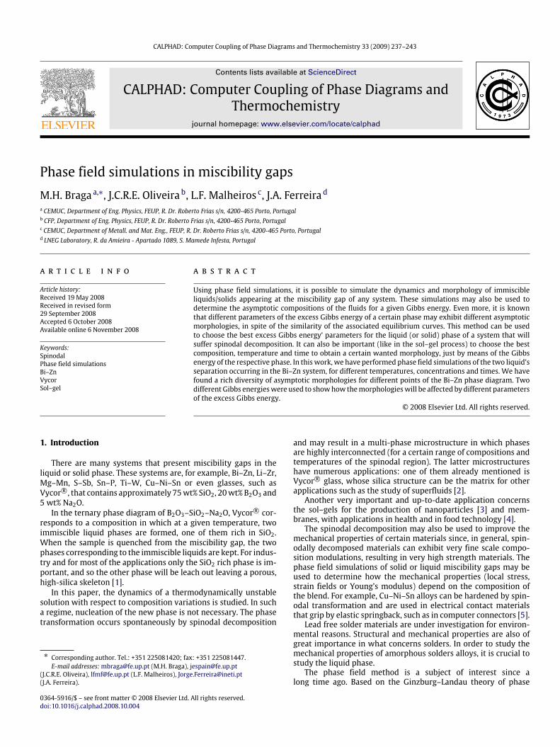
Fig. 1. The zoom of the miscibility gap occurring in the liquid region as well asits spinodal region obtained from Gibbs energy by [16] after [14]. The scale limits,which are the values of φ for each temperature obtained with the simulations,are represented by the two opposing circles in the phase diagram miscibility gapcurve (x(Liquid#1, Zn) and x(liquid#2, Zn)); points in squares present variations ofthe simulated asymptotic morphology at different temperatures and compositionsshown in Fig. 3.

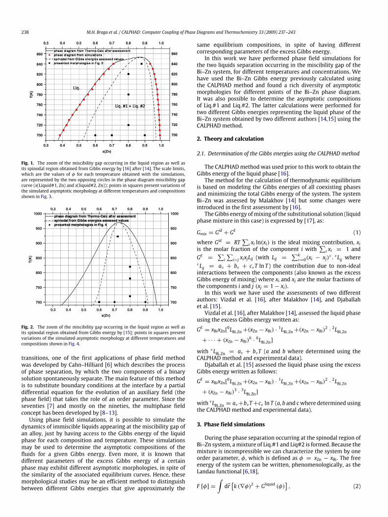
Fig. 2. The zoom of the miscibility gap occurring in the liquid region as well asits spinodal region obtained from Gibbs energy by [15]; points in squares presentvariations of the simulated asymptotic morphology at different temperatures andcompositions shown in Fig. 4.

transitions, one of the first applications of phase field methodwas developed by Cahn–Hilliard [6] which describes the processof phase separation, by which the two components of a binarysolution spontaneously separate. The main feature of this methodis to substitute boundary conditions at the interface by a partialdifferential equation for the evolution of an auxiliary field (thephase field) that takes the role of an order parameter. Since theseventies [7] and mostly on the nineties, the multiphase fieldconcept has been developed by [8–13].Using phase field simulations, it is possible to simulate the

dynamics of immiscible liquids appearing at the miscibility gap ofan alloy, just by having access to the Gibbs energy of the liquidphase for each composition and temperature. These simulationsmay be used to determine the asymptotic compositions of thefluids for a given Gibbs energy. Even more, it is known thatdifferent parameters of the excess Gibbs energy of a certainphase may exhibit different asymptotic morphologies, in spite ofthe similarity of the associated equilibrium curves. Hence, thesemorphological studies may be an efficient method to distinguishbetween different Gibbs energies that give approximately the

same equilibrium compositions, in spite of having differentcorresponding parameters of the excess Gibbs energy.In this work we have performed phase field simulations for

the two liquids separation occurring in the miscibility gap of theBi–Zn system, for different temperatures and concentrations. Wehave used the Bi–Zn Gibbs energy previously calculated usingthe CALPHAD method and found a rich diversity of asymptoticmorphologies for different points of the Bi–Zn phase diagram.It was also possible to determine the asymptotic compositionsof Liq.#1 and Liq.#2. The latter calculations were performed fortwo different Gibbs energies representing the liquid phase of theBi–Zn system obtained by two different authors [14,15] using theCALPHAD method.

2. Theory and calculation

2.1. Determination of the Gibbs energies using the CALPHAD method

The CALPHADmethod was used prior to this work to obtain theGibbs energy of the liquid phase [16].The method for the calculation of thermodynamic equilibrium

is based on modeling the Gibbs energies of all coexisting phasesand minimizing the total Gibbs energy of the system. The systemBi–Zn was assessed by Malakhov [14] but some changes wereintroduced in the first assessment by [16].The Gibbs energy ofmixing of the substitutional solution (liquid

phase mixture in this case) is expressed by [17], as:

Gmix = Gid + GE (1)

where Gid = RT∑i xi ln(xi) is the ideal mixing contribution, xi

is the molar fraction of the component i with∑i xi = 1 and

GE =∑i∑i>j xixjLij (with Lij =

∑kν=0(xi − xj)

ν . νLij whereνLij = aν + bν + cνT ln T ) the contribution due to non-idealinteractions between the components (also known as the excessGibbs energy of mixing) where xi and xj are the molar fractions ofthe components i and j (xj = 1− xi).In this work we have used the assessments of two different

authors: Vizdal et al. [16], after Malakhov [14], and Djaballahet al. [15].Vizdal et al. [16], after Malakhov [14], assessed the liquid phase

using the excess Gibbs energy written as:

GE = xBixZn[0LBi,Zn+(xZn − xBi) ·1LBi,Zn+(xZn − xBi)

2·2LBi,Zn

+ · · · + (xZn − xBi)6 · 6LBi,Zn]

with νLBi,Zn = aν + bνT (a and b where determined using theCALPHAD method and experimental data).Djaballah et al. [15] assessed the liquid phase using the excess

Gibbs energy written as follows:

GE = xBixZn[0LBi,Zn+(xZn − xBi) ·1LBi,Zn+(xZn − xBi)

2·2LBi,Zn

+ (xZn − xBi)3 · 3LBi,Zn]

with νLBi,Zn = aν+bνT+cν ln T (a, b and cwhere determined usingthe CALPHAD method and experimental data).

3. Phase field simulations

During the phase separation occurring at the spinodal region ofBi–Zn system, amixture of Liq.#1 and Liq#2 is formed. Because themixture is incompressible we can characterize the system by oneorder parameter, φ, which is defined as φ = xZn − xBi. The freeenergy of the system can be written, phenomenologically, as theLandau functional [6,18],

F [φ] =∫dEr[k (∇φ)2 + Gliquid (φ)

], (2)

M.H. Braga et al. / CALPHAD: Computer Coupling of Phase Diagrams and Thermochemistry 33 (2009) 237–243 239

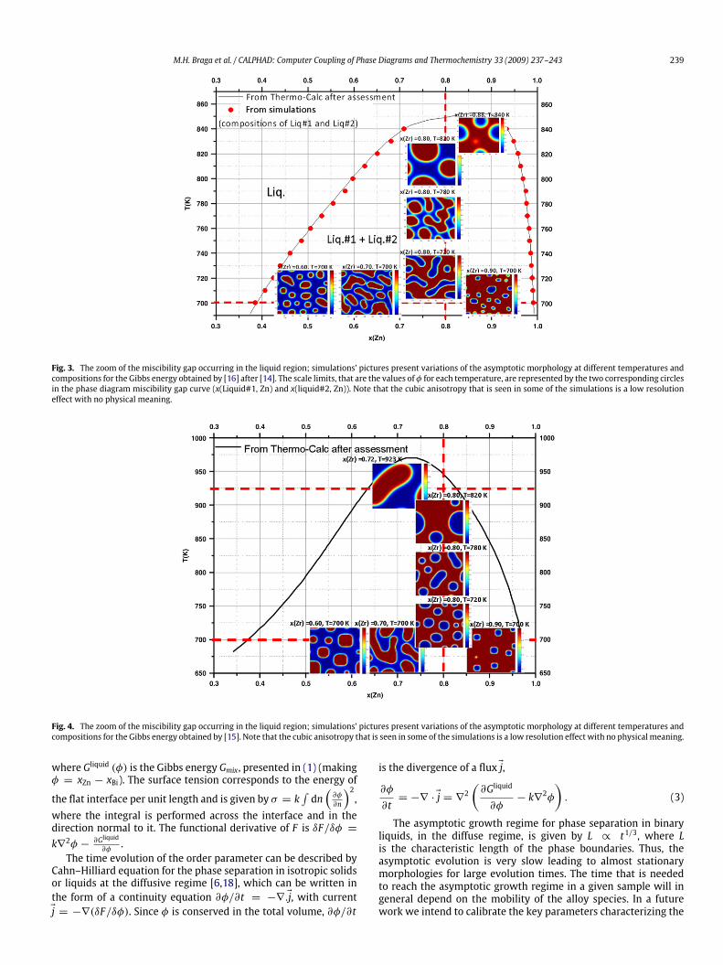
Fig. 3. The zoom of the miscibility gap occurring in the liquid region; simulations’ pictures present variations of the asymptotic morphology at different temperatures andcompositions for the Gibbs energy obtained by [16] after [14]. The scale limits, that are the values of φ for each temperature, are represented by the two corresponding circlesin the phase diagram miscibility gap curve (x(Liquid#1, Zn) and x(liquid#2, Zn)). Note that the cubic anisotropy that is seen in some of the simulations is a low resolutioneffect with no physical meaning.

Fig. 4. The zoom of the miscibility gap occurring in the liquid region; simulations’ pictures present variations of the asymptotic morphology at different temperatures andcompositions for the Gibbs energy obtained by [15]. Note that the cubic anisotropy that is seen in some of the simulations is a low resolution effect with no physical meaning.

where Gliquid (φ) is the Gibbs energy Gmix, presented in (1) (makingφ = xZn − xBi). The surface tension corresponds to the energy of

the flat interface per unit length and is given by σ = k∫dn(∂φ

∂n

)2,

where the integral is performed across the interface and in thedirection normal to it. The functional derivative of F is δF/δφ =k∇2φ − ∂Gliquid

∂φ.

The time evolution of the order parameter can be described byCahn–Hilliard equation for the phase separation in isotropic solidsor liquids at the diffusive regime [6,18], which can be written inthe form of a continuity equation ∂φ/∂t = −∇.Ej, with currentEj = −∇(δF/δφ). Since φ is conserved in the total volume, ∂φ/∂t

is the divergence of a fluxEj,

∂φ

∂t= −∇ ·Ej = ∇2

(∂Gliquid

∂φ− k∇2φ

). (3)

The asymptotic growth regime for phase separation in binaryliquids, in the diffuse regime, is given by L ∝ t1/3, where Lis the characteristic length of the phase boundaries. Thus, theasymptotic evolution is very slow leading to almost stationarymorphologies for large evolution times. The time that is neededto reach the asymptotic growth regime in a given sample will ingeneral depend on the mobility of the alloy species. In a futurework we intend to calibrate the key parameters characterizing the

240 M.H. Braga et al. / CALPHAD: Computer Coupling of Phase Diagrams and Thermochemistry 33 (2009) 237–243

Fig. 5. Differentmorphologies obtained for the same composition x(Zn)= 0.8 and time, at different indicated temperatures, to allowa comparison between themorphologiesobtained with different Gibbs energies (Gibbs1 by [14,16] and Gibbs2 [15]). Time increases from left to right starting above (time in each large square is the same). The scalescorrespond to the values of φ.

system by performing a detailed quantitative study of the timeevolution of L in the simulations and a subsequent comparisonwith the observed one in different system samples.In Eq. (3) changing the time scale can scale out k. In fact the

same dynamics can be obtained with a different surface tensionby changing the size of the simulation box accordingly. Hence, theasymptoticmorphology of the system is just a function of theGibbsenergy and not of the value of k.In the alloy system, the atoms of A and B (Bi and Zn in this

case) can exchange position only locally (not over large distances),leading then to a diffusive transport of the order parameter.We have integrated (3) using a standard finite-difference

method [19]. In all simulations we have used initial randomconditions for φ and k = 1.

4. Results and discussion

In Figs. 1 and 2 both the miscibility gap and spinodal curves,obtained after the assessments of [14,16] and [15] respectively, canbe observed. In Fig. 1 the points corresponding to the asymptoticvalues of x(Liq.#1, Zn) and x(Liq.#2, Zn), obtained in this work byphase field simulations, can also be observed.In Fig. 3, themiscibility gap curve of the Bi–Zn system is shown.

A good agreement, between the equilibrium curve calculatedin [16] and the one obtained by the simulations was found asexpected. Here, the simulations’ images for different compositions

and temperatures represent the asymptotic morphologies of theBi–Zn system near the equilibrium configuration. It can be seenthat the size and shape of the domains change considerablywith temperature for the same concentration, and with theconcentration, for the same temperature.In Fig. 4 equivalent results to those of Fig. 3 are shown. It can

be observed that the morphologies corresponding to the sametemperatures and compositions are considerably different. Forinstance, interconnected structures may appear in a region of themiscibility gap of Fig. 4 where in Fig. 3 round shaped domainsappear.By the analysis of the asymptotic morphologies shown inside

the miscibility gap, it can be seen that for the compositions neareach side of the spinodal line (Figs. 1–4), there is a matrix of themore abundant liquid and inside thismatrix, isolated round shapeddomains of the other liquid phase appear. Concerning the system’compositions that are more in the middle of the spinodal region,for the same temperature as the previously referredmorphologies,interconnected domains can be observed. These interconnecteddomains have many applications and the identification of thecompositions for which they appear is crucial [20,21].Note for example that, for x(Zn) = 0.8 in Fig. 3, interconnected

domains appear at least for T ≤ 780 K.Only round shapeddomainscan be observed for x(Zn) = 0.8 in Fig. 4. If the phase diagramsand spinodal lines are compared, it can be seen that the lattercomposition in the miscibility gap of Fig. 1 corresponds to thecenter of the spinodal region and that at T = 720 K it is clear

M.H. Braga et al. / CALPHAD: Computer Coupling of Phase Diagrams and Thermochemistry 33 (2009) 237–243 241

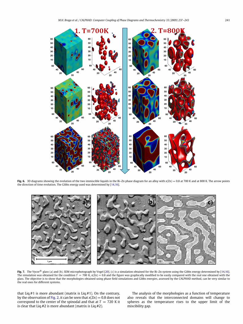
Fig. 6. 3D diagrams showing the evolution of the two immiscible liquids in the Bi–Zn phase diagram for an alloy with x(Zn)= 0.8 at 700 K and at 800 K. The arrow pointsthe direction of time evolution. The Gibbs energy used was determined by [14,16].

Fig. 7. The Vycor r© glass (a) and (b). SEM microphotograph by Vogel [20]. (c) is a simulation obtained for the Bi–Zn system using the Gibbs energy determined by [14,16].The simulation was obtained for the condition T = 700 K, x(Zn) = 0.8 and the figure was graphically modified to be easily compared with the real one obtained with theglass. The objective is to show that the morphologies obtained using phase field simulations and Gibbs energies, assessed by the CALPHAD method, can be very similar tothe real ones for different systems.

that Liq.#1 is more abundant (matrix is Liq.#1). On the contrary,by the observation of Fig. 2, it can be seen that x(Zn)= 0.8 does notcorrespond to the center of the spinodal and that at T = 720 K itis clear that Liq.#2 is more abundant (matrix is Liq.#2).

The analysis of the morphologies as a function of temperaturealso reveals that the interconnected domains will change tospheres as the temperature rises to the upper limit of themiscibility gap.

242 M.H. Braga et al. / CALPHAD: Computer Coupling of Phase Diagrams and Thermochemistry 33 (2009) 237–243

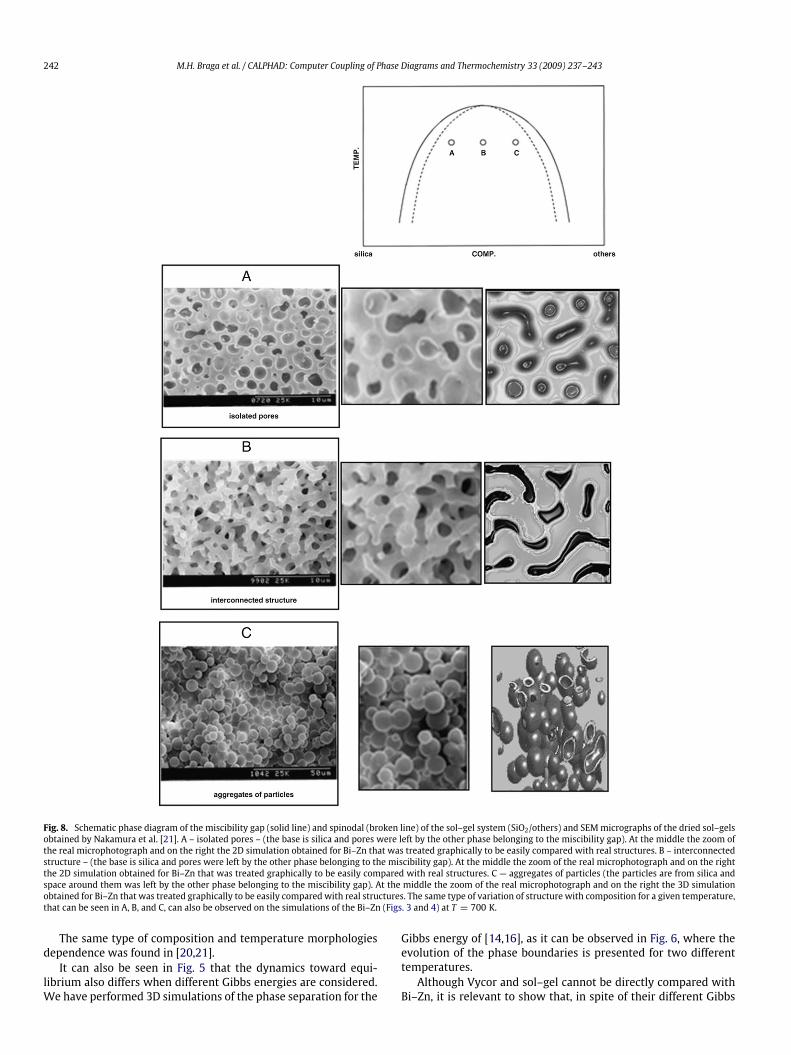
Fig. 8. Schematic phase diagram of the miscibility gap (solid line) and spinodal (broken line) of the sol–gel system (SiO2/others) and SEMmicrographs of the dried sol–gelsobtained by Nakamura et al. [21]. A – isolated pores – (the base is silica and pores were left by the other phase belonging to the miscibility gap). At the middle the zoom ofthe real microphotograph and on the right the 2D simulation obtained for Bi–Zn that was treated graphically to be easily compared with real structures. B – interconnectedstructure – (the base is silica and pores were left by the other phase belonging to the miscibility gap). At the middle the zoom of the real microphotograph and on the rightthe 2D simulation obtained for Bi–Zn that was treated graphically to be easily compared with real structures. C — aggregates of particles (the particles are from silica andspace around them was left by the other phase belonging to the miscibility gap). At the middle the zoom of the real microphotograph and on the right the 3D simulationobtained for Bi–Zn that was treated graphically to be easily compared with real structures. The same type of variation of structure with composition for a given temperature,that can be seen in A, B, and C, can also be observed on the simulations of the Bi–Zn (Figs. 3 and 4) at T = 700 K.

The same type of composition and temperature morphologiesdependence was found in [20,21].It can also be seen in Fig. 5 that the dynamics toward equi-

librium also differs when different Gibbs energies are considered.We have performed 3D simulations of the phase separation for the

Gibbs energy of [14,16], as it can be observed in Fig. 6, where theevolution of the phase boundaries is presented for two differenttemperatures.Although Vycor and sol–gel cannot be directly compared with

Bi–Zn, it is relevant to show that, in spite of their different Gibbs

M.H. Braga et al. / CALPHAD: Computer Coupling of Phase Diagrams and Thermochemistry 33 (2009) 237–243 243

energies, similar morphologies can be observed in correspondingrelative positions of the miscibility gap and spinodal regions. Thisfact enhances the possible applications of the method.Figs. 7 and 8 show comparisons between our Bi–Zn simulated

morphologies (obtainedwith the Gibbs energy [14,16]) and similarones for observed samples of Vycor r© [20] and sol–gel [21],respectively.

5. Conclusions

Using phase field simulations, the dynamics of the twoimmiscible liquids appearing on the phase diagram of the Bi–Znsystem was studied. Good agreement between the miscibility gapcurve determined by the simulations and the one obtained by theCALPHAD method was found, as expected.It was found a rich diversity of asymptotic morphologies for

different points of the Bi–Zn phase diagram.We have compared the morphologies for two different

Gibbs energies determined by Calphad method and found verydifferent morphologies for the same times, concentrations andtemperatures. Thus, it can be concluded that the differentmorphologies and the time it takes to reach them is a signature ofthe calculated excess Gibbs energy parameters for a given system.It could also be verified the similarities between the simulated

structures and those observed in different real systems, such asVycor r© glass and sol–gel.It can be pointed out, that for a given temperature, the

morphologies of the Bi–Zn system depend on the composition ina similar way as those observed in the sol–gel system, especiallythe morphologies obtained with one of the Gibbs energies.The results obtained in this work show that using the Gibbs

energies, obtained for example with the CALPHAD method andphase field simulations, we have a straightforward method todetermine the morphologies of the miscibility gap as a function

of the concentration, temperature and time. This method may beuseful to find the best structures, depending on the applicationsand purposes; for instance, for the fabrication of nanoparticles.

Acknowledgements

The authors would like to acknowledge the COST MP0602action: ‘‘Advanced SolderMaterials for High-Temperature Applica-tion — their nature, design, process and control in a multiscaledomain’’.

References

[1] M.H. Bartl, K. Gatterer, H.P. Fritzer, S. Arafa, Spectrochim. Acta A 57 (2001)1991–1999.

[2] B. Peter, B. Paul, L. Gavin, C. Lee, M. Akira, I. Osamu, M. Pinaki, Phys. Lett. A 310(4) (2003) 311–321.

[3] A. Bouchara, G. Mosser, G.J.A.A. Soler-Illia, J.-Y. Chane-Ching, C. Sanchez,J. Mater. Chem. 14 (2004) 2347–2354.

[4] P. Schurtenberger, Nanotech 2005, California, U.S.A., May 8–12, 2005.[5] S.M. Allen, E.L. Thomas, The Structure of Materials, Wiley MIT, 1999, pp. 374.[6] J.W. Cahn, J.E. Hilliard, J. Chem. Phys. 28 (2) (1958) 258.[7] J.S. Langer, H. Müller-Krumbhaar, Acta Metall. 26 (1978) 1681, 1689, 1697.[8] L.Q. Chen, A.G. Khachaturyan, Acta Metall. Mater 39 (11) (1991).[9] A.A.Wheeler,W.J. Boettinger, G.B.Mc Fadden, Phys. Rev. A 45 (10) (1992) 7424.[10] G. Caginalp, E. Socolovsky, SIAM J. Sci. Comput. 15 (1) (1994) 106.[11] R. Kobayashi, Physica D 63 (3,4) (1993) 410.[12] A.A. Wheeler, B.T. Murray, R.J. Schaefer, Physica D 66 (1,2) (1993) 243.[13] J. Steinbach, F. Pezzolla, B. Nestler, M. Seeßelberg, R. Prieler, G.J. Schmitz,

J.L.L. Rezende, Physica D 94 (1996) 135.[14] D.V. Malakhov, CALPHAD 24 (2000) 1–14.[15] Y. Djaballah, L. Bennour, F. Bouharkat, A. Belgacem-Bouzida, Modeling. Simul.

Mater. Sci. Eng. 13 (2005) 361–369.[16] J. Vizdal, M.H. Braga, A. Kroupa, K.W. Richter, D. Soares, L.F. Malheiros,

J. Ferreira, CALPHAD 31 (2007) 438–448.[17] O. Redlich, A. Kister, Ind. Eng. Chem. 40 (1948) 411–420.[18] A.J. Bray, Adv. Phys. 43 (1994) 357–458.[19] J.C.R.E. Oliveira, C.J.A.P. Martins, P.P. Avelino, Phys. Rev. D 71 (2005) 083509.[20] W. Vogel, Chemistry of the Glass, The American Ceramics Society, 1985, pp. 83.[21] N. Nakamura, R. Takahashi, S. Sato, T. Sodesawa, S. Yoshida, Phys. Chem. Chem.

Phys. 2 (2000) 4983–4990.