petrel tips&tricks from scm - scm e&p solutions, inc. · pdf filefault model quality...

K n o w l e d g e W o r t h S h a r i n g

Petrel TIPS&TRICKS from SCM

Petrel is a mark of Schlumberger

4801 Woodway Drive, Suite 150W • Houston, TX 77056 • www.scminc.com • [email protected]

© 2011 SCM E&P Solutions, Inc.

1

Fault Model Quality Control Most Petrel projects are faulted. This means that fault models must be built and then checked for accuracy in almost every 3D Grid that is built. If you are new to Petrel or have only built a few faulted frameworks, this Tips & Tricks will provide a guide for checking the quality of your faults as well as hints for speeding the QC process. If you are an experienced Petrel modeler and have built many faulted structural frameworks, then this Tips & Tricks will provide a quick review of the methods commonly used to check fault accuracy and perhaps remind you of issues you may have forgotten.

We are often asked how much of the Petrel modeling effort is spent on QC and our answer is always 35% to 40%. This usually surprises those new to modeling and those on the sidelines watching the modeling process. Old time modelers will sometimes question these numbers for a while but when asked about visually checking the quality of each surface, fault, or property they build, checking its statistics, its histograms, how it honors input data, etc. they quickly realize how much time they spend on QC. The QC must be done when the object is built, not later, for to move on with a poor product means you are only postponing the redo and likely increasing the amount that must ultimately be re‐done.

Review – Fault Data and Modeling Methods

A quick review of fault data and modeling methods will make sure everyone has the same background when we discuss QC.

Typical Fault Data

Fault sticks – The intersection of a seismic section and a fault plane defines a line. If that line is digitized and stored in the seismic interpretation it is called a fault stick. Multiple sticks representing one fault are normally grouped together in one file. Sometimes these are converted from sticks to “horizons” so they can be output just as an interpreted horizon is.

Fault polygons – The intersection of a fault plane with a structural surface defines a line refereed to as a fault trace and is stored as a polygon in mapping systems. The polygon is usually a closed figure having two sides, up‐thrown and down‐thrown. Often polygons for multiple faults are joined together into one large convoluted shaped polygon. These large multi‐fault polygons must be separated at the bifurcations before being used in the fault modeling process.

Fault cuts – The intersection of a well bore and the fault plane is a point. These points are normally stored in the tops file as a fault cut. The fault cut is used in fault modeling to ensure that the fault plane stays correctly positioned along the well bore.

Fault gaps – The fault gap is the space between the up‐thrown structure surface and the down‐thrown surface. Vertical faults will have no gap, reversed faults will have an overlap region and normal fault will have a gap. Interpreted horizons usually have approximate gaps and because of the difficulty in interpreting near faults will sometimes be wider or narrower than the actual gap.




2

Fault face – For a single structural surface this is the portion of the fault plan between the up‐thrown side of the fault and the down‐thrown side of the fault. When an interpreted horizon is gridded, the grid nodes will have values calculated in the fault gap that approximate the fault plane. These we will refer to as the fault face. Because the gap is normally a little wider than actual the calculated fault face will be a little gentler than actual.

Modeling Methods

Automatic Key Pillar Construction – Automatic implies that something is done for you and with fault modeling this means the program generates the Key Pillars. This automation only happens when using Fault Sticks or Fault Polygons as the primary input. It can also happen when using 2D Grids representing the fault surfaces as primary input (often built from: sticks, sticks in horizon format, polygons, or a combination of data types). The quality of these automatically generated Key Pillars is highly variable with polygons usually producing the worst and 2D Grids the best Key Pillars. The fault sticks selected for automatic conversion to Key Pillars must not cross one another and should be aligned as near as possible in the down dip direction.

Digitizing Key Pillars – Digitizing means that data, representing a fault, is displayed and then X‐Y‐Z locations captured from that data as Key Pillar shape points. The authors have found that digitizing can be quite fast and generally produces the best quality fault model. Digitizing is used when fault sticks will not create good Pillars automatically, when fault data have not been captured but cross sections through the interpretation (showing the gap and displacement) demonstrate where the fault should be located, or when 2D Structure grids show the fault position in a 3D or 2D window as a break in slope.

Quality Control Check of the Fault Model

QC methods vary from individual to individual and project to project. Also, the QC used to check a single fault may not be the same QC used to check a group of faults. The discussion below is separated into QC checks for single, small groups, and all fault models and for Pillar gridded faults.

QC – The Single Fault Model

Each fault’s model should be looked at and either signed off as being acceptable or fixed to make it acceptable. The fault’s model is usually constructed using one set of data although often several types of data will exist for the fault. QC is initially done with the data used to build the fault model. QC is not complete until the fault’s model is checked against all data available for the fault.

QC the Primary Fault Data

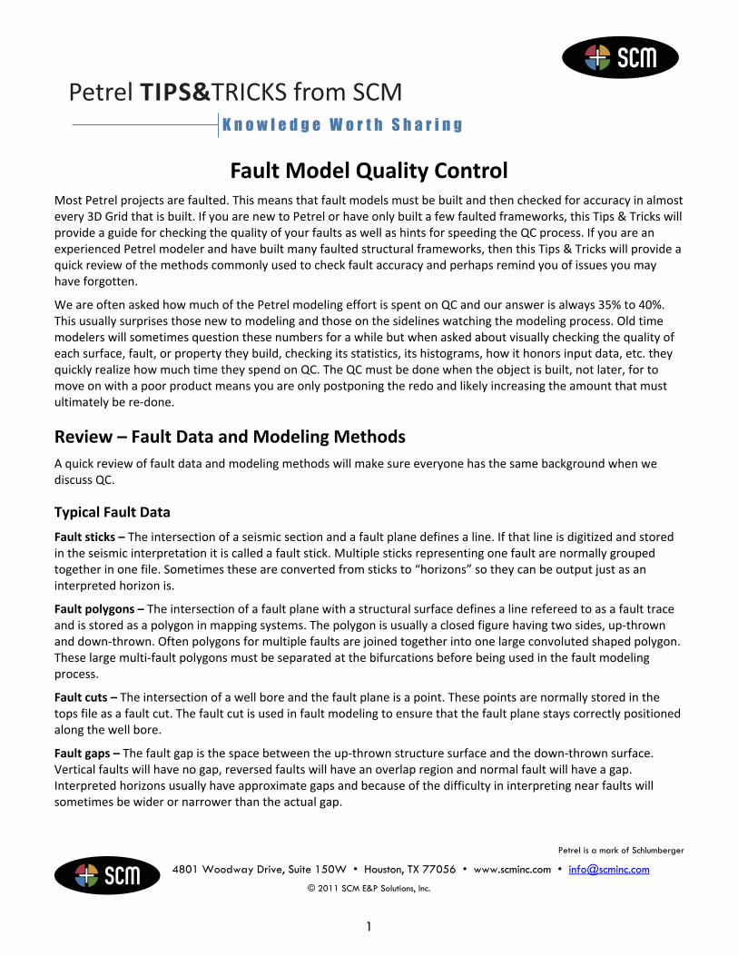
In a 3D window, display the fault model for only one fault. Display the data used to build that fault model. Rotate the display so you are at one end of the fault model and looking directly down the Key Pillars on that end. Work your way across the fault checking:

To see that the Key Pillars run through the center of the data.




3

Figure: Key Pillars viewed from above show the fault shifted off the data (top) and moved to the “center” of the data (bottom).

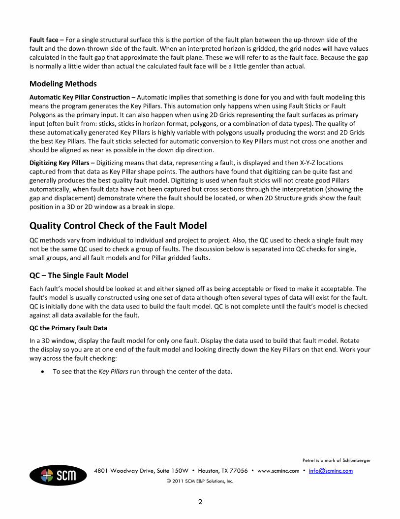
If the data curves significantly in the vertical direction then see if shape points (3 or 5) are needed to allow the Pillar to bend with the data.

Figure: Two shape point Key Pillars do not always honor the form of the fault (top) and the use of three shape points will sometimes do a better job (bottom).

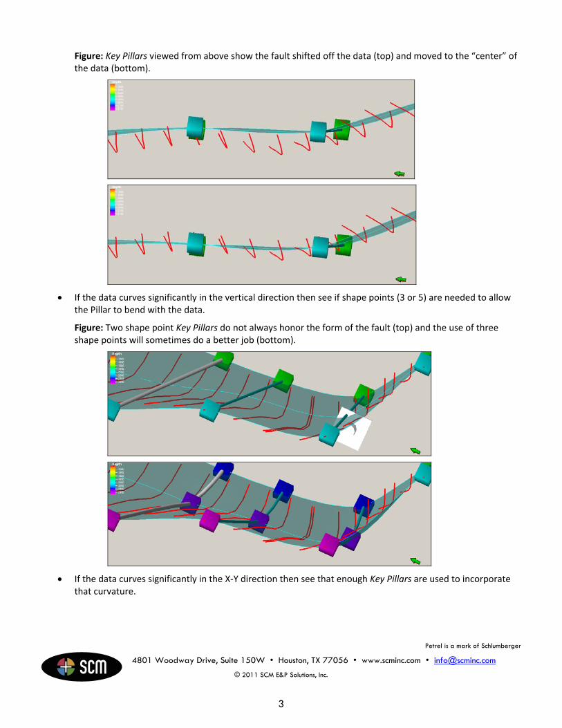
If the data curves significantly in the X‐Y direction then see that enough Key Pillars are used to incorporate that curvature.




4

Figure: Too few Key Pillars to follow the fault’s curvature in X‐Y (top) and enough Key Pillars to honor fault form (bottom).

To see that Key Pillars and Shape Points are spaced as far apart as possible while still honoring the changing trends of the data. You do not want to and won’t be able to honor every “kink” in the fault, only its trends.

Figure: Key Pillars too close together to allow easy edit and QC (top) and properly positioned (bottom).

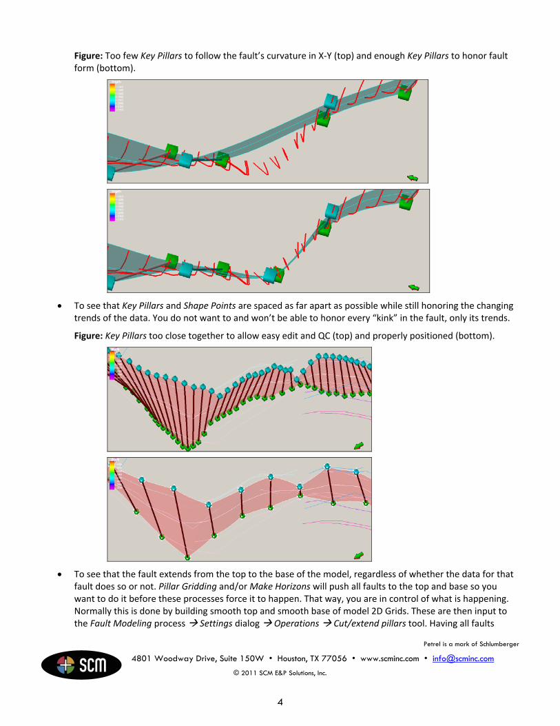
To see that the fault extends from the top to the base of the model, regardless of whether the data for that fault does so or not. Pillar Gridding and/or Make Horizons will push all faults to the top and base so you want to do it before these processes force it to happen. That way, you are in control of what is happening. Normally this is done by building smooth top and smooth base of model 2D Grids. These are then input to the Fault Modeling process Settings dialog Operations Cut/extend pillars tool. Having all faults




5

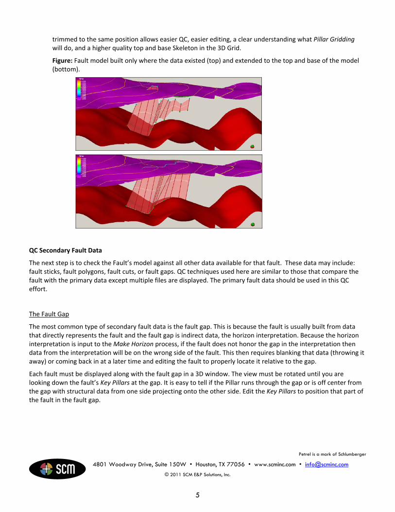
trimmed to the same position allows easier QC, easier editing, a clear understanding what Pillar Gridding will do, and a higher quality top and base Skeleton in the 3D Grid.

Figure: Fault model built only where the data existed (top) and extended to the top and base of the model (bottom).

QC Secondary Fault Data

The next step is to check the Fault’s model against all other data available for that fault. These data may include: fault sticks, fault polygons, fault cuts, or fault gaps. QC techniques used here are similar to those that compare the fault with the primary data except multiple files are displayed. The primary fault data should be used in this QC effort.

The Fault Gap

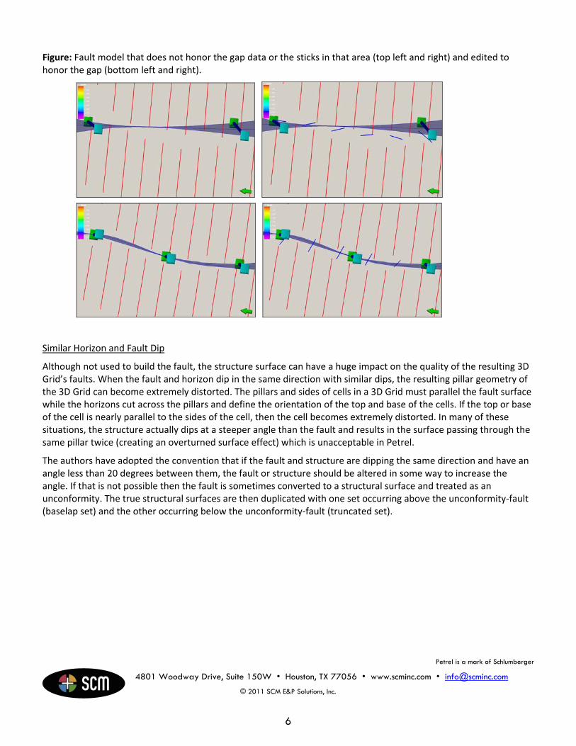
The most common type of secondary fault data is the fault gap. This is because the fault is usually built from data that directly represents the fault and the fault gap is indirect data, the horizon interpretation. Because the horizon interpretation is input to the Make Horizon process, if the fault does not honor the gap in the interpretation then data from the interpretation will be on the wrong side of the fault. This then requires blanking that data (throwing it away) or coming back in at a later time and editing the fault to properly locate it relative to the gap.

Each fault must be displayed along with the fault gap in a 3D window. The view must be rotated until you are looking down the fault’s Key Pillars at the gap. It is easy to tell if the Pillar runs through the gap or is off center from the gap with structural data from one side projecting onto the other side. Edit the Key Pillars to position that part of the fault in the fault gap.




6

Figure: Fault model that does not honor the gap data or the sticks in that area (top left and right) and edited to honor the gap (bottom left and right).

Similar Horizon and Fault Dip

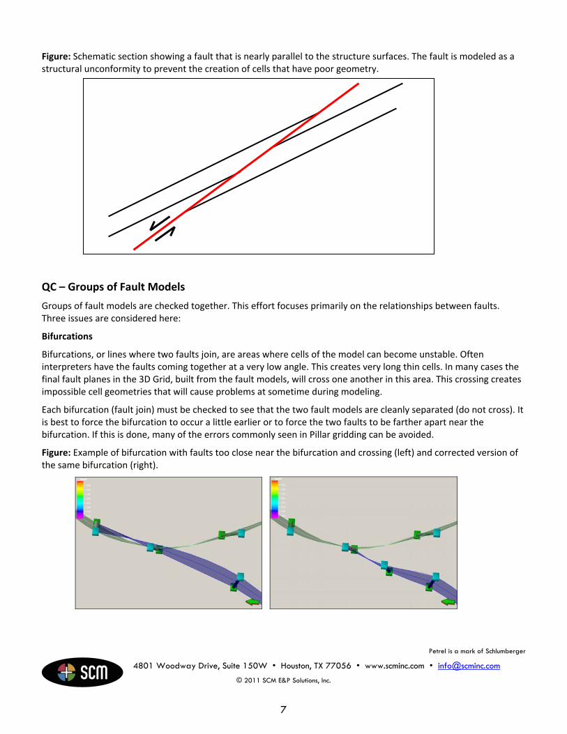
Although not used to build the fault, the structure surface can have a huge impact on the quality of the resulting 3D Grid’s faults. When the fault and horizon dip in the same direction with similar dips, the resulting pillar geometry of the 3D Grid can become extremely distorted. The pillars and sides of cells in a 3D Grid must parallel the fault surface while the horizons cut across the pillars and define the orientation of the top and base of the cells. If the top or base of the cell is nearly parallel to the sides of the cell, then the cell becomes extremely distorted. In many of these situations, the structure actually dips at a steeper angle than the fault and results in the surface passing through the same pillar twice (creating an overturned surface effect) which is unacceptable in Petrel.

The authors have adopted the convention that if the fault and structure are dipping the same direction and have an angle less than 20 degrees between them, the fault or structure should be altered in some way to increase the angle. If that is not possible then the fault is sometimes converted to a structural surface and treated as an unconformity. The true structural surfaces are then duplicated with one set occurring above the unconformity‐fault (baselap set) and the other occurring below the unconformity‐fault (truncated set).




7

Figure: Schematic section showing a fault that is nearly parallel to the structure surfaces. The fault is modeled as a structural unconformity to prevent the creation of cells that have poor geometry.

QC – Groups of Fault Models

Groups of fault models are checked together. This effort focuses primarily on the relationships between faults. Three issues are considered here:

Bifurcations

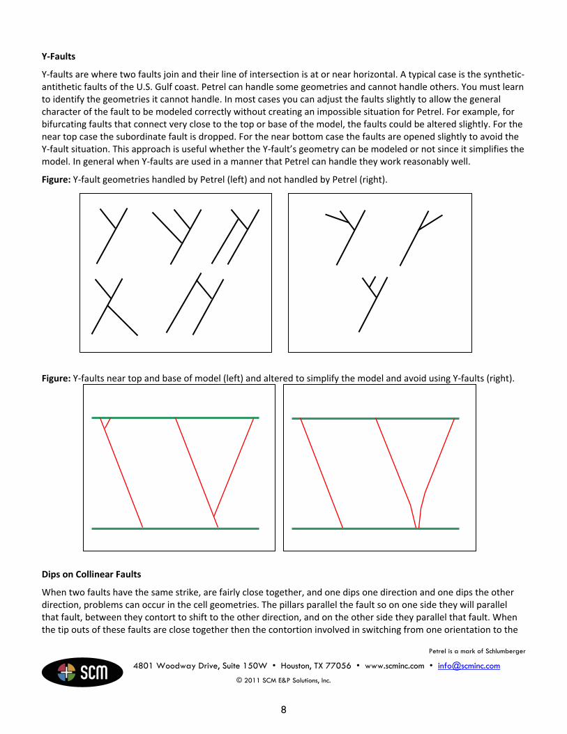
Bifurcations, or lines where two faults join, are areas where cells of the model can become unstable. Often interpreters have the faults coming together at a very low angle. This creates very long thin cells. In many cases the final fault planes in the 3D Grid, built from the fault models, will cross one another in this area. This crossing creates impossible cell geometries that will cause problems at sometime during modeling.

Each bifurcation (fault join) must be checked to see that the two fault models are cleanly separated (do not cross). It is best to force the bifurcation to occur a little earlier or to force the two faults to be farther apart near the bifurcation. If this is done, many of the errors commonly seen in Pillar gridding can be avoided.

Figure: Example of bifurcation with faults too close near the bifurcation and crossing (left) and corrected version of the same bifurcation (right).




8

Y‐Faults

Y‐faults are where two faults join and their line of intersection is at or near horizontal. A typical case is the synthetic‐antithetic faults of the U.S. Gulf coast. Petrel can handle some geometries and cannot handle others. You must learn to identify the geometries it cannot handle. In most cases you can adjust the faults slightly to allow the general character of the fault to be modeled correctly without creating an impossible situation for Petrel. For example, for bifurcating faults that connect very close to the top or base of the model, the faults could be altered slightly. For the near top case the subordinate fault is dropped. For the near bottom case the faults are opened slightly to avoid the Y‐fault situation. This approach is useful whether the Y‐fault’s geometry can be modeled or not since it simplifies the model. In general when Y‐faults are used in a manner that Petrel can handle they work reasonably well.

Figure: Y‐fault geometries handled by Petrel (left) and not handled by Petrel (right).

Figure: Y‐faults near top and base of model (left) and altered to simplify the model and avoid using Y‐faults (right).

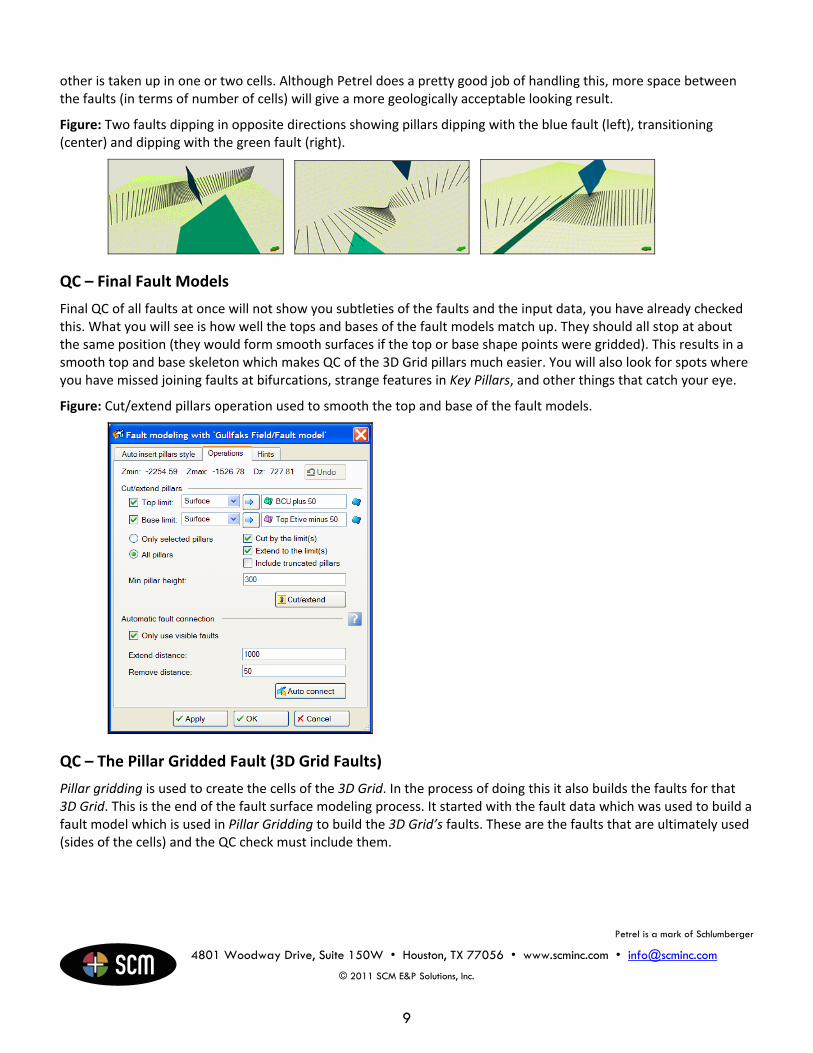
Dips on Collinear Faults

When two faults have the same strike, are fairly close together, and one dips one direction and one dips the other direction, problems can occur in the cell geometries. The pillars parallel the fault so on one side they will parallel that fault, between they contort to shift to the other direction, and on the other side they parallel that fault. When the tip outs of these faults are close together then the contortion involved in switching from one orientation to the




9

other is taken up in one or two cells. Although Petrel does a pretty good job of handling this, more space between the faults (in terms of number of cells) will give a more geologically acceptable looking result.

Figure: Two faults dipping in opposite directions showing pillars dipping with the blue fault (left), transitioning (center) and dipping with the green fault (right).

QC – Final Fault Models

Final QC of all faults at once will not show you subtleties of the faults and the input data, you have already checked this. What you will see is how well the tops and bases of the fault models match up. They should all stop at about the same position (they would form smooth surfaces if the top or base shape points were gridded). This results in a smooth top and base skeleton which makes QC of the 3D Grid pillars much easier. You will also look for spots where you have missed joining faults at bifurcations, strange features in Key Pillars, and other things that catch your eye.

Figure: Cut/extend pillars operation used to smooth the top and base of the fault models.

QC – The Pillar Gridded Fault (3D Grid Faults)

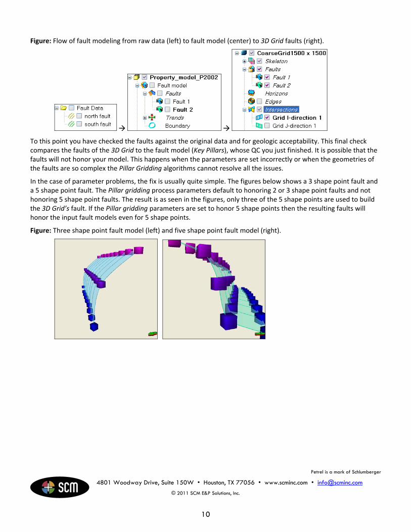
Pillar gridding is used to create the cells of the 3D Grid. In the process of doing this it also builds the faults for that 3D Grid. This is the end of the fault surface modeling process. It started with the fault data which was used to build a fault model which is used in Pillar Gridding to build the 3D Grid’s faults. These are the faults that are ultimately used (sides of the cells) and the QC check must include them.




10

Figure: Flow of fault modeling from raw data (left) to fault model (center) to 3D Grid faults (right).

To this point you have checked the faults against the original data and for geologic acceptability. This final check compares the faults of the 3D Grid to the fault model (Key Pillars), whose QC you just finished. It is possible that the faults will not honor your model. This happens when the parameters are set incorrectly or when the geometries of the faults are so complex the Pillar Gridding algorithms cannot resolve all the issues.

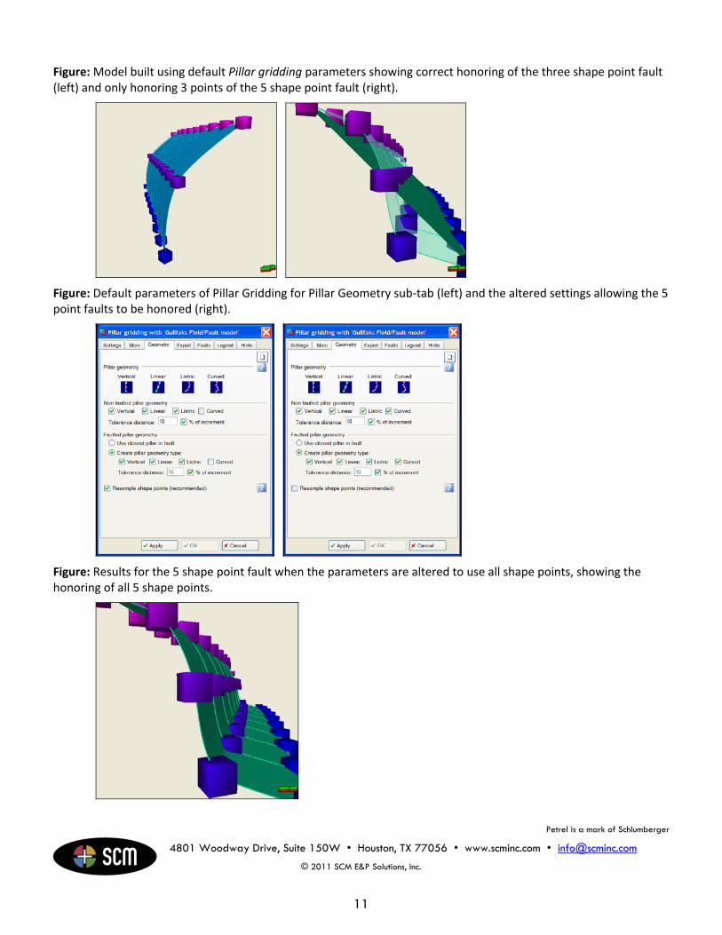
In the case of parameter problems, the fix is usually quite simple. The figures below shows a 3 shape point fault and a 5 shape point fault. The Pillar gridding process parameters default to honoring 2 or 3 shape point faults and not honoring 5 shape point faults. The result is as seen in the figures, only three of the 5 shape points are used to build the 3D Grid’s fault. If the Pillar gridding parameters are set to honor 5 shape points then the resulting faults will honor the input fault models even for 5 shape points.

Figure: Three shape point fault model (left) and five shape point fault model (right).




11

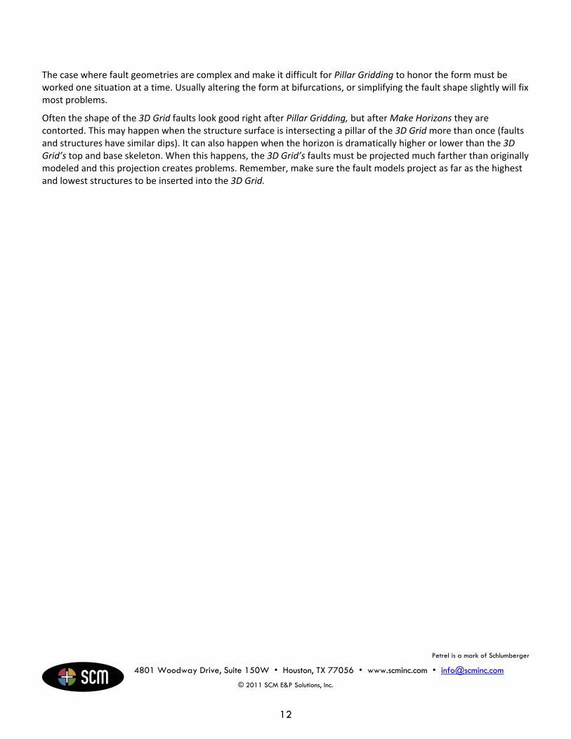
Figure: Model built using default Pillar gridding parameters showing correct honoring of the three shape point fault (left) and only honoring 3 points of the 5 shape point fault (right).

Figure: Default parameters of Pillar Gridding for Pillar Geometry sub‐tab (left) and the altered settings allowing the 5 point faults to be honored (right).

Figure: Results for the 5 shape point fault when the parameters are altered to use all shape points, showing the honoring of all 5 shape points.




12

The case where fault geometries are complex and make it difficult for Pillar Gridding to honor the form must be worked one situation at a time. Usually altering the form at bifurcations, or simplifying the fault shape slightly will fix most problems.

Often the shape of the 3D Grid faults look good right after Pillar Gridding, but after Make Horizons they are contorted. This may happen when the structure surface is intersecting a pillar of the 3D Grid more than once (faults and structures have similar dips). It can also happen when the horizon is dramatically higher or lower than the 3D Grid’s top and base skeleton. When this happens, the 3D Grid’s faults must be projected much farther than originally modeled and this projection creates problems. Remember, make sure the fault models project as far as the highest and lowest structures to be inserted into the 3D Grid.

petrel tips&tricks from scm - scm e&p solutions, inc. · pdf filefault model quality...

Documents