petrel tips&tricks from scm - scminc.com · petrel tips&tricks from scm create fault...

Petrel is a mark of Schlumberger

4801 Woodway Drive, Suite 150W • Houston, TX 77056 • www.scminc.com • [email protected]

© 2010 SCM E&P Solutions, Inc.

1

K n o w l e d g e W o r t h S h a r i n g

Petrel TIPS&TRICKS from SCM

Create Fault Polygons and Map

This is the first in a series of TIPS&TRICKS focused on the geophysical and seismic aspects of Petrel. Petrel combines geophysics, geology and reservoir engineering modules to enable a full seismic to simulation workflow. Reservoir modeling practices can be made more efficient if the interpreter is involved in modeling early in the game. The “Create fault polygons and map” operation found in the Operations tab of the Settings window for the seismic horizon helps create high quality geologically sound maps, is also a good QC tool and an excellent introduction to reservoir modeling.

Fault exclusion polygons are a part of nearly every seismic interpretation workflow. They are commonly used in map presentations of seismic horizon interpretations and can even be used in the fault modeling process in Petrel. An interpreter has, in the past, had to manually draw exclusion polygons by hand. This was done by digitizing polygons around null values or areas of gaps in the interpretation. This can prove to be a painstaking process with only a moderate number of faults.

Petrel offers a seismic interpretation horizon operation, available for the first time in the 2009 release that automatically constructs polygons from seismic fault interpretations. Fault segments and a horizon interpretation created in the seismic interpretation process are used as inputs. Accurate fault polygons are created by intersecting the seismic horizon interpretation data with the fault interpretation. The only requirements are that the faults must be collected together in a folder and the seismic horizon must be in Petrel seismic interpretation format.

The output is a surface that is gridded through the faults and fault exclusion polygons. A faulted 3D grid model of the surface is also created as an added bonus. This can be used to QC the seismic interpretation to ensure that it is geologically sound and to identify any problem area prior to larger scale modeling.

Zones can be added to the resulting model to perform gross rock volume (GRV) calculations using the volumetric calculation process.

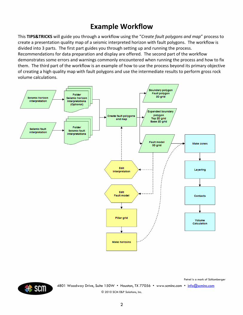
Example Workflow This TIPS&TRICKS will guide you through a workflow using the “Create fault polygons and map” process to create a presentation quality map of a seismic interpreted horizon with fault polygons. The workflow is divided into 3 parts. The first part guides you through setting up and running the process. Recommendations for data preparation and display are offered. The second part of the workflow demonstrates some errors and warnings commonly encountered when running the process and how to fix them. The third part of the workflow is an example of how to use the process beyond its primary objective of creating a high quality map with fault polygons and use the intermediate results to perform gross rock volume calculations.




2

Prepare data and displays The “Convert fault polygons and map” process is available under Settings > Operations > Convert points/polygons/surfaces for seismic interpreted horizons only. Seismic horizons and faults are interpreted in Petrel or imported from ASCII files. If they interpreted in Petrel, there is no further preparation of the horizons, except to optionally group them into a common folder. Creating a folder of

grouped horizons allows you to use the “Similar objects” option to perform the operation on all of the horizons in the folder. If the seismic horizons were imported as points or polygon lines it may be necessary to convert them to Petrel seismic interpretation format.

The only required input for the operation is a folder containing the seismic fault interpretations to be used. The folder should contain only those seismic fault interpretations that intersect the seismic horizon interpretation you are running the process on. The process will issue a warning if some of the seismic fault interpretations in the folder do not intersect the seismic horizon interpretation. The process will fail with no output if none of the faults intersect the seismic horizon interpretation.

It is recommended by the author that a 2D or 3D window also be prepared at this time. If there is problem with the pillar gridding, it will be highlighted but only temporarily. A pop-up dialog box will appear when a problem is encountered. You must respond to it before continuing. In the case of a problem in pillar gridding, the problem areas are highlighted in a 2D or 3D display. You must make a mental note of the problem pillars because the highlighting will disappear after responding to the pop-up warning dialog.

The data used in the following examples is the Gulfaks demo data set available to all current Petrel license holders.

Figure – Folder containing faults to be Figure – Faults displayed in 3D window used in operation for pillar grid QC




3

Run Operation There are two data inputs to consider for the operation. One is for the seismic fault interpretation folder. It is the only required input for the operation to run. The other is optional and is used for the geometry of the output results of the operation. This optional input can be either a seismic cube, seismic interpreted horizon, or a regular surface. If no surface is input for the optional geometry, it will be determined from the selected seismic horizon interpretation data.

You can follow the recommended workflow outlined below using the Petrel provided Gulfaks demo data set to run the operation.

1. Double click on the seismic horizon interpretation name (Top Ness) in the Input tab.

2. Go to the Operations tab of the settings dialogue window and expand the “Convert points/polygons/surfaces” folder.

3. Click on “Create fault polygons and map”.

Operations > Convert points/polygons/surfaces > Create fault polygons and map

4. Use the blue arrow to enter the faults folder containing the seismic fault interpretation (Fault Sticks).

5. This example will not use the optional object to use for the XY limits and geometry of resulting surfaces. We will let the input seismic horizon interpretation determine the geometry.

6. Uncheck the “Clean faults segments” option. It is recommended that you run the operation without this option activated. This option resamples and decimates the original interpretation with no control over the parameters and the results can be dramatically different from the original




4




5

interpretation. The figures below illustrate this effect on the example data set. The same data was input into the process for both figures, the only difference being the activation of the “Clean faults segments” option. It is better to run the operation without the cleaning option and let the program inform you of problems with the pillar gridding. You can then make corrections to the problem areas and rerun the operation. An example of this procedure will be presented in the QC and edit workflow.

Figure – Clean fault segments active Figure – Clean fault segments not active

7. Put a check mark in the box next to the option labeled “Keep intermediate results”. The author recommends that this option be activated to validate the process. The intermediate results are also required in the last part of the example workflow. The final results consist of a folder in the Input tab that initially contains a boundary polygon file, a 2D grid file, and a fault polygon file. These alone are not enough to properly QC and edit the process.

8. Click on Run to execute the process.

The process actually consists of several auxiliary processes run in sequence in the background to arrive at the final result. The results of these auxiliary processes are referred to as the intermediate results and are saved by activating the “Keep intermediate results” option. The intermediate results consist of 3 additional objects found in the Input tab folder created by the process. In addition to the final results you will find an expanded version of the boundary along with a top and base surface. The top and base surfaces are smoothed versions of the original input seismic horizon interpretation that have been shifted up and down in depth. These are used to condition the fault interpretation when creating the fault model. The faults are clipped and extended to the top and base surfaces. This narrows the focus of the model on the surface of interest and helps avoid any problematic fault connections above or below the surface of interest when pillar gridding.

Figure – Intermediate results saved in the Input tab

There will also be a new 3D grid with a fault model in the Models tab that bears the name of the seismic horizon interpretation used in the process. The model will be used for 2 purposes in this workflow example. First we will use it to QC the results of the pillar gridding process that runs in the background. We will also use it in the last part of the workflow to create a layered model to use for calculating GRV.

Figure – Intermediate results saved in the Models tab




6

QC/edit results The process was run on all of the seismic horizon interpretations in a folder (Horizons) for the example.

Figure – Seismic horizon interpretation folder One of the horizons in the folder (Seabed) did not intersect any of the fault interpretations. The following series of 4 error messages were issued and no output was created for the horizon. For the example we answer yes to the last dialogue box to continue the process to the next horizon in the folder.

The message below is issued when there are some fault interpretations that do not intersect the seismic horizon interpretation. This was the Base Cretaceous horizon in the example. If you answer Yes, the bad faults are dropped and the process continues without them. If you answer No, the process is stopped and nothing is saved.




7

The message below is issued if the process has difficulty auto connecting the faults in the fault model as is the case with the Etive horizon in the example data set. This is where you need the fault interpretation display described in the Prepare Data and Displays section of this article. You must make a mental note of where the problem areas are because the fault model and the highlighted problem pillars disappear from the display when the process ends. Answering yes allows the process to run and create the output data. If you selected to keep the intermediate results, you can now QC the results of the fault model and 3D grid.




8

The figure below shows the QC and editing workflow. The problem area is highlighted and indentified during the process execution. You can clearly see, in the figures below, an unwanted kink in the fault model and a peculiar structure in the 3D grid. There are two ways to approach this problem. One is to manually edit the fault model, rerun pillar gridding, rerun make horizons, and create fault polygons from the 3D grid on your own. This workflow requires some knowledge of the Petrel modeling process. The author recommends another method for the interpreting geophysicist. Simply edit the seismic fault interpretation and rerun the “Make fault polygons and map” process. This has two benefits. One, it is much simpler than the manual method mentioned previously. Another is that the seismic interpretation is made model centric. The seismic interpretation enables the modeling process instead of complicating it. The modeling process is made more efficient because the problem area in pillar gridding have been indentified and fixed in the interpretation stage.

1. Make a mental note of the problem areas as the process runs. 2. Answer Yes to the notification dialogue to continue the process. 3. Display the fault interpretation along with the new fault model in a 3D window. 4. Make the Seismic interpretation process active. 5. Click on the icon to enter Fault interpretation mode. 6. Select the problem segment and delete it. 7. Rerun the “Make fault polygons and map” process.

High quality, geologically accurate fault polygons are now available to produce presentation maps.




9

Gross Rock Volume Calculations The intermediate results from the process are essential in QC and editing and can also be used to calculate gross rock volume. The following example leads you through a workflow to add zones and layering, and create fluid contacts for volume calculations using the 3D grid output from the process above. A. Depth convert 3D grid The resulting 3D grid is currently in the time domain. The model must be converted to depth to run the volume calculation workflow.

1. Make sure the correct model is active in the Models tab (Top Tarbert). 2. Double click on the Depth convert 3D grid process under Structural modeling in the Processes tab.

Processes > Structural modeling > Depth convert 3D grid 3. Select “Velocity Model 1” as the velocity model. 4. Click on OK to run the domain conversion.

B. Add zones Zones can quickly be added to the 3D grid created in the intermediate results by running the Make zones process. Well top picks are input to build conformable zones. This works well as log as the zones stay within +- 50 depth units of the original interpretation. More than that and the top and base surface created by the process must be adjusted to extend the faults a short distance beyond the highest and lowest zone.




10

1. Make sure the correct model is active in the Models tab (Top Tarbert). 2. Double click on the Make zones process found under Structural modeling in the Processes tab.

Processes > Structural modeling > Make zones 3. Insert 3 rows, one for each well top pick to be used (Tarbert2, Tarbert1, Top Ness) 4. Make the input type Conformable.

C. Layering Once the zones are created, the layering process can be run. Each individual zone may be layered as desired.

1. Make sure the correct model is active. 2. Double click on the Layering process under Structural modeling in the Processes tab.

Process > Structural modeling > Layering 3. Set the layering method to Proportional 4. Set the number of layers to 10 for each zone.




11

D. Create fluid contact Contacts can be added using the Make Contacts process. An oil/water and a gas/oil contact are the most common types of contacts used. The contact can have a constant value or be represented by a gridded surface.

1. Make sure the correct model is active. 2. Double click on the Make contacts process under Structural modeling in the Processes tab.

Processes > Structural modeling > Make Contacts 3. Click on the Create new radio button and enter a name for the contact set. 4. Insert 2 new rows by clicking on the icon. 5. Click on the first one to highlight it and make it active. Set the Contact type to Gas oil contact and

name it something like GOC. 6. Enter a constant value for the gas/oil contact. (-1800 works well with the Top Tarbert example.) 7. Click on the second row to make it active and make the contact type Oil water contact. Name it

something like OWC. 8. Enter a constant value for the oil/water constant. (-1850 works well for the Top Tarbert example.) 9. Click on OK and the contacts are made.

E. Run volumetrics At this point you have a model with multiple zones and layering. You may also have created fluid contacts. It is possible now to calculate the gross rock volume of the 3D grid. Calculations from the 3D grid are more accurate than results from more traditional 2D mapping methods most interpreters are accustomed to.

1. Double click on the Volume calculation process under Utilities in the Processes tab. Processes > Utilities > Volume calculation

2. Enter a case name. 3. Select the 3D grid for input.




12

4. Go to the Properties tab and enter the contacts. Do this by highlighting the fluid contact from the 3D grid in the Models tab and using the blue arrow to insert it.

5. Go to the General properties tab. Make sure the net to gross and porosity are set to a constant 1. 6. Go to the Oil properties tab and make sure the water saturation is set to a constant of 0. 7. Go to the Output tab under the Results tab and select Bulk volume, HCPV oil, and HCPV gas volume

height maps to output. 8. Select to output a spreadsheet report. 9. Click on Report settings and select to report Bulk volume, HCPV oil, and HCPV gas. Click on OK. 10. Click on Run and the volumes are calculated for each zone and each segment (fault block)




13




14

Conclusion The primary object of the “Make fault polygons and map” process is to produce high quality fault polygons and associated maps for presentation in an exploration project. The traditional workflow is to manually digitize polygons around gaps in the interpretation. Petrel 2009 automates this workflow with a new process. This new process creates a polygon file and 2D surface grid and places them in a new folder in the Input tab. The polygons are created from a 3D grid and fault model that are made in the background. The background, or intermediate, results can optionally be saved during the process and used for QC and editing purposes. This also serves as an interpreter’s introduction to the reservoir modeling workflows in Petrel. The interpreter gains a new respect for the modeler by running this process and viewing the results, especially if it does not work the first time and the interpretation needs to be modified for the process to run successfully. The intermediate results can also be used to calculate preliminary gross rock volumes in exploration type workflows.

petrel tips&tricks from scm - scminc.com · petrel tips&tricks from scm create fault...

Documents