FORWARD MODELING AND INVERSION

OF DC RESISTIVITY AND MMR DATA

by

PETER ROBERT MCGILLIVRAY

A THESIS SUBMITTED IN PARTIAL FULFILLMENT OF

THE REQUIREMENTS FOR THE DEGREE OF

DOCTOR OF PHILOSOPHY

in

THE FACULTY OF GRADUATE STUDIES

Department of Geophysics and Astronomy

We accept this thesis as conforming

to the required standard

THE UNIVERSITY OF BRITISH COLUMBIA

January 1992

© Peter McGillivray, 1992

In presenting this thesis in partial fulfilment of the requirements for an advanced

degree at the University of British Columbia, I agree that the Library shall make it

freely available for reference and study. I further agree that permission for extensive

copying of this thesis for scholarly purposes may be granted by the head of my

department or by his or her representatives. It is understood that copying or

publication of this thesis for financial gain shall not be allowed without my written

permission.

______________________

Department of

_____________________

The University of British ColumbiaVancouver, Canada

Date /_

DE-6 (2188)

Abstract

This thesis is a presentation of research that has addressed the forward and inverse problems

for the DC resistivity and magnetometric resistivity (MMR) experiments. The emphasis has been on

the development of practical numerical procedures for solving problems involving a large number of

data and unknowns. The relative value, in terms of information content, of the different data sets

arising from DC resistivity or MMR experiments has also been emphasized. For the purposes of this

work, a two-dimensional conductivity structure was assumed, although the results can be extended

to three-dimensions.

The first part of this research focused on the development of numerical algorithms to accurately

and efficiently solve the forward problem. A forward modeling algorithm based on the integrated

finite difference discretization was first developed. The algorithm was designed to model a variety

of different responses, including pole-pole, pole-dipole, dipole-dipole and MMR measurements

for surface, cross-borehole and borehole-to-surface arrays. Complex conductivity structures and

topography can also be specified. The high accuracy of the algorithm was demonstrated by comparing

forward modeled results with analytic solutions for different conductivity models. The algorithm was

then used in the development of a multi-grid procedure for iteratively computing DC resistivity

responses. The multi-grid algorithm makes use of a sequence of grids of increasing fineness to

accelerate convergence. Testing of the multi-grid algorithm demonstrated its value as a fast and

accurate solver for the DC resistivity problem. The use of non-coextensive grids was also found

to be useful for achieving higher resolution in the vicinity of singularities and rapid changes in the

conductivity. The multi-grid approach was used in the development of a novel adaptive grid design

procedure that iteratively refines an initial numerical grid. The application of this algorithm to the

modeling of DC resistivity responses for different conductivity structures illustrated the usefulness

H

of the approach, and demonstrated the need for assessing the accuracy of a numerically computed

solution.

The second part of this research focused on the calculation of the sensitivities of the modeled

responses to changes in the model parameters — quantities that are essential to the solution of the non

linear inverse problem. A study of the available techniques for numerically computing sensitivities

was carried out to determine the most suitable approach. Based on this study, an adjoint formulation

for the 2D resistivity and MMR problem was developed. A comparison of these numerically computed

sensitivities to ones obtained by perturbing the model parameters verified the accuracy of the approach.

The final part of this research focused on the solution of the inverse problem. The inversion

of DC resistivity data has traditionally employed a coarse parameterization of the model to reduce

the non-uniqueness of the problem. Although this can succeed in reducing the non-uniqueness, it

can also lead to problems of poor stability and slow convergence. In this work, a strategy of using

a fine parameterization of the model was adopted. The resulting non-uniqueness was reduced by

requiring that the final solution minimize a global norm of the model. Computational problems

were addressed using a re-parameterization based on a generalized subspace approach. The use

of linearized information to avoid computing a large number of forward solutions was examined.

The resulting generalized subspace algorithm was tested by inverting synthetic data sets generated

for pole-pole, pole-dipole, dipole-dipole and cross-borehole electrode configurations. The success

of these inversions demonstrated the stability and efficiency of the generalized subspace approach.

Synthetic MMR data Sets were also inverted, both individually and in a joint inversion with pole-

pole resistivity data. The results indicated that the additional information provided by the magnetic

field data can help to better resolve the subsurface. An E-SCAN pole-pole field data Set was also

inverted, and a solution that delineated two conductors was obtained. The solution was consistent

with geological cross-Sections that were available for the study area.

lii

Table of Contents

Abstract.

List of Figures ix

Acknowledgments xv

Introduction 1

1.1 The DC resistivity experiment 1

1.1.1 Field procedure 2

1.1.2 Applications 3

1.1.3 Relationship between electrical resistivity and other parameters 4

1.1.4 Interpretation 5

1.2 The magnetometric resisrivity (MMR) experiment 7

1.2.1 Field procedure 7

1.2.2 Applications 8

1.2.3 Processing and interpretation 9

1.3 The E-SCAN pole-pole experiment 10

1.4 Solution of large-scale forward and inverse problems 12

1.4.1 Solution of the forward problem 12

1.4.2 Calculation of sensitivities 14

1.4.3 Solution of the inverse problem

iv

15

2 Finite Difference Solution of the 2D Pole-pole Resistivity and MMR Forward Problems. . . 17

2.1 Introduction 17

2.2 Mathematical formulation

2.2.1 Transformed problem

2.3 Discretization of the forward problem

2.3.1 Discretization to obtain the FD operator and truncation error

2.3.2 Approximation of boundary conditions

2.3.3 Assembly of the mathx system

2.4 Singularity removal

2.4.1 Modeling of secondary potentials

2.4.2 Discretization of secondary potential problem

2.5 Method of solving the discrete matrix equations

2.6 Inversion of the Fourier transform

2.7 Examples

2.8 Modeling of topographic responses

2.9 Calculation of MMR. responses

2.10 Examples

2.11 Conclusions

3 Multi-grid and Multi-Level Solution of the DC Resistivity Forward Problem

3.1 Introduction

3.2 Multi-grid solution of the forward problem

3.2.1 Basic two-level multi-grid iteration

3.2.2 General N-level multi-grid iteration

V

18

19

20

21

25

26

26

27

28

33

34

36

45

47

48

49

51

51

52

53

56

3.2.3 Convergence rate of the N-level multi-grid iteration 59

3.2.4 Computation work for the N-level multi-grid solution 59

3.2.5 Variations on the basic multi-grid iteration 60

3.2.6 Applications of multi-grid methods to DC resistivity modeling 63

3.2.7 Examples — convergence rates for various models and operators 69

3.3 The multi-level adaptive technique 77

3.3.1 Multi-level adaptive technique 78

3.3.2 Example 82

3.4 Conclusions 83

4 Adaptive Grid-design Using the Multi-grid Approach 85

4.1 Introduction 85

4.2 Numerical error and grid design considerations 86

4.2.1 Factors controlling truncation error strengths 87

4.3 Adaptive solution of the numerical forward problem 89

4.3.1 Two-level multi-grid approach to adaptive grid design 90

4.3.2 Efficiency of the adaptive multi-grid approach 93

4.4 Examples 96

4.5 Conclusions 106

5 Numerical calculation of sensitivities 108

5.1 Introduction 108

5.2 Solution of the non-linear inverse problem 109

5.3 Solution of the non-linear parametric inverse problem Ill

vi

5.4 Calculation of Differential Sensitivities 113

5.4.1 Perturbation approach 113

5.4.2 Sensitivity equation approach 113

5.4.3 Adjoint equation approach 117

5.4.4 Example — Calculation of sensitivities for the 1 D resistivity problem . . . 119

5.5 Adjoint sensitivities for the 2D resistivity and MMR problem 129

5.5.1 Choice of model and model parameterization 129

5.5.2 Calculation of 2D pole-pole sensitivities 130

5.5.3 Calculation of 2D MIVIR sensitivities 135

5.6 Conclusions 138

6 Subspace Inversion of DC Resistivity and MMR Data 140

6.1 Introduction 140

6.2 Generalized subspace inversion 141

6.2.1 Non-linear least-squares approach 142

6.2.2 Minimization of a global model norm 143

6.2.3 Computational aspects of the Gauss-Newton approach . 144

6.2.4 Subspace formulation 147

6.2.5 Use of additional basis vectors — the generalized subspace approach 148

6.3 Regularization of the inverse problem 152

6.3.1 Choice of weighting matrix 153

vii

6.3.2 Weighting schemes for cells along grid boundaries

6.3.3 Non-uniform mesh spacing

6.3.4 Determining the optimum ridge regression parameter.

6.3.5 Problems related to regularization

6.3.6 Subspace steepest descent algorithm

6.4 Inversion of DC resistivity and MMR data

6.4.1 Choice of data for the inversion

6.4.2 Development of the 2D inversion algorithm

6.5 Examples

6.5.1 Inversion of pole-pole responses

6.5.2 Inversion of pole-dipole and dipole-dipole responses

6.5.3 Inversion of cross-borehole pole-pole responses . .

6.5.4 Inversion of MMR responses

6.5.5 Joint inversion of MMR and pole-pole resistivity responses

6.5.6 Inversion of E-SCAN field data

6.6 Conclusions

7 Summary and Conclusions

References

155

156

158

161

163

165

165

166

168

169

178

179

186

189

190

195

197

Appendix A — Adjoint Equation Formulation for the Frequency Domain EM Problem 208

200

viii

List of Figures

1.1 Electrode configuration for the pole-pole, pole-dipole and dipole-dipole arrays 2

1.2 Electrode configuration for an E-SCAN survey 11

2.1 Two dimensional finite difference grid used to discretize the transformed DC resistivity

problem 21

2.2 Finite difference operator used in the discretization of the transformed DC resistivity

problem 22

2.3 Quarterspace problem used to illustrate the accuracy problems associated with a

non-conservative discretization of the secondary source 30

2.4 Secondary potentials computed using conservative and non-conservative discretization

schemes compared to the analytic solution for the model in Figure 2.3 32

2.5 Finite difference grid used to solve the transformed resistivity problem 36

2.6 Detail of the finite difference grid in Figure 2.5 37

2.7 Quarterspace model used to test the results of the finite difference algorithm 37

2.8 Forward modeled results for the quarterspace model in Figure 2.7 38

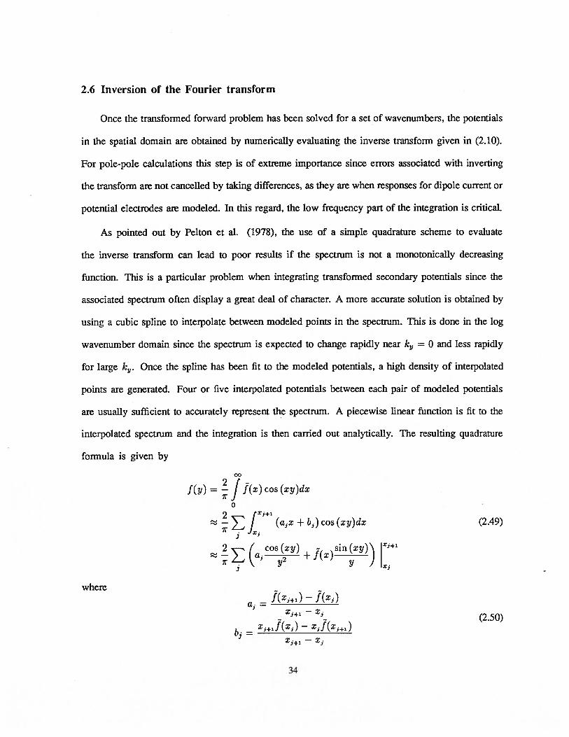
2.9 Vertical dike model used to test the results of the finite difference algorithm 39

2.10 Forward modeled results for the vertical dike model in Figure 2.9 40

2.11 Layered earth model used to test the results of the finite difference algorithm 41

2.12 Forward modeled results for the layered earth model in Figure 2.11 42

2.13 Conductive prism model used to test the accuracy of the inverse Fourier cosine

transform 43

2.14 Forward modeled results for the conductive prism model in Figure 2.13 44

ix

2.15 Cliff model used to illustrate the calculation of terrain effects using the finite difference

algorithm 45

2.16 Forward modeled results for the cliff model in Figure 2.15 46

2.17 Numerically modeled B and B fields for the layered earth problem in Figure 2.11,

and B field for the quarterspace problem in Figure 2.7 49

3.1 Examples of a coarse grid !H and fine grid 1h for use in the two-level multi-grid

algorithm 54

3.2 Examples of a four-level multi-grid iteration using the “V-cycle” and the “W-cycle”

scheme 58

3.3 Example of a four-level FMG multi-grid iteration 62

3.4 Full weighting restriction from fine grid to coarse grid 64

3.5 Injection from fine grid to coarse grid 67

3.6 Bilinear interpolation from the coarse grid to the fine grid 68

3.7 Higher order operator based interpolation from the coarse grid to the fine grid 68

3.8 Two prism problem used to illustrate the convergence properties of the multi-grid

forward modeling algorithm 69

3.9 Coarsest grid in the multi-grid discretization of the problem in Figure 3.8 70

3.10 Convergence of the two-level multi-grid solution for the problem in Figure 3.8 71

3.11 Results of a two, three and four-level multi-grid solution for the problem in Figure 3.8. . 72

3.12 Convergence rates of the four-level multi-grid algorithm for different multi-grid transfer

operators 73

3.13 Convergence rates of the four-level multi-grid algorithm for different relaxation

schemes 74

3.14 Convergence rates of the four-level multi-grid algorithm for different wavenumbers and

conductivity contrasts 75

x

3.15 Four-level multi-grid solution for the problem in Figure 3.8 76

3.16 Comparison of the solutions computed using a direct solver and the four-level

multi-grid solver for the problem in Figure 3.8 77

3.17 A sequence of three coextensive grids used in the standard multi-grid iteration 78

3.18 A sequence of three non-coextensive grids. The finer grids extend over only a

sub-region of the coarser grids in the sequence 79

3.19 A sequence of composite grids where hanging nodes have been tied in to the rest of the

grid using rotated finite difference operators 81

3.20 Composite grid generated using the MLAT algorithm for the problem in Figure 3.8. . . 82

3.21 Transformed secondary potentials computed using the MLAT algorithm for the problem

in Figure 3.8 83

4.1 Conductivity model used to illustrate the use of the two-level adaptive multi-grid

algorithm 96

4.2 Sequence of four coarse grids generated by the adaptive multi-grid algorithm for the

model in Figure 4.1 97

4.3 Profiles of the total potentials computed for the sequence of four grids generated in the

first example 98

4.4 Relative error computed at the control node for each of iteration of the adaptive

solution of the problem in Figure 4.2 99

4.5 Two resistive prism problem 100

4.6 First, second, third and fifth coarse grids generated by the adaptive multi-grid algorithm

for the model in Figure 4.5 101

4.7 Profiles of the secondary potentials computed for the sequence of grids in Figure 4.5.. 102

4.8 Relative error computed at the control node for each of iteration of the adaptive

solution of the problem in Figure 4.5 102

xi

4.9 Model used in the third two-level adaptive multi-grid example 103

4.10 Sequence of three coarse grids generated by the adaptive multi-grid algorithm for the

model in Figure 4.9 104

4.11 Profiles of the secondary potentials computed for the sequence of three grids in Figure

4.10 105

4.12 Relative error computed at the control node for each of iteration of the adaptive

solution of the problem in Figure 4.9 105

5.1 Conductivty model and transformed surface potential used in the 1D resistivity

example 123

5.2 Sensitivity as a function of depth for A = 0.005 computed using the perturbation

method, the sensitivity equation method, and the adjoint equation method 124

5.3 Perturbed model for step length parameter s = 1.0 and s = 2.0 128

5.4 Transformed potential as a function of the step length parameter .s computed using the

tracking sensitivity approach 129

5.5 Parameterization of the 1000 2m uniform halfspace model that was used to demonstrate

the accuracy of sensitivities calculated using the adjoint equation approach 133

5.6 Pole-pole sensitivities computed for the 1000 fm uniform halfspace problem shown in

Figure 5.5 134

5.7 Sensitivities computed for the By response from an MMR experiment for the 1000 c2m

uniform halfspace problem shown in Figure 5.5 137

6.1 Cpu time required to perform a Golub-Reinsch singular value decomposition of an

M x M matrix as a function of the number of parameters M 146

6.2 Parameterization of a 2D model 158

6.3 Data misfit plotted against the ridge regression parameter R generated through the

course of a non-linear line search 160

xli

6.4 Non-linear data misfit and linearized approximation to the data misfit plotted against the

ridge regression parameter ,u 160

6.5 Model and parameterization used in the solution of the inverse problem 168

6.6 Cross-sections showing the log resistivities (log10(p)) obtained by inverting pole-pole

resistivity data for the model in Figure 6.5 170

6.7 Convergence of the generalized subspace algorithm for the results in Figure 6.6. . . . 171

6.8 Cross-section showing the log resistivities obtained after 40 iterations of the two basis

vector subspace formulation. Pole-pole resistivity data for the model in Figure 6.5 were

used in the inversion 172

6.9 Convergence of the generalized subspace algorithm for the results in Figure 6.8. . . . 172

6.10 Results of the generalized subspace inversion of pole-pole data using additional

“blocky” basis vectors 173

6.11 Convergence of the generalized subspace algorithm for the results in Figure 6.10. . . 174

6.12 Cross-sections showing the log resistivities obtained by inverting pole-pole resistivity

data for the model in Figure 6.5 for two different choices of a3 175

6.13 Convergence of the generalized subspace algorithm for two different choices of a5. . 176

6.14 Cross-sections showing the log resistivities obtained by inverting pole-pole resistivity

data for the model in Figure 6.5 177

6.15 Convergence of the generalized subspace algorithm for the result in Figure 6.14. . . . 177

6.16 Cross-sections showing the log resistivities obtained by inverting pole-dipole and

dipole-dipole data sets for the model in Figure 6.5 178

6.17 Model and parameterization used in the cross-borehole inversion examples 180

6.18 Cross-section showing the log resistivities obtained by inverting cross-borehole

pole-pole resistivity data for the model in Figure 6.17 181

6.19 Convergence of the generalized subspace algorithm for the result in Figure 6i8. . . . 182

XII 1

6.20 Model and numerical grid used to generate the synthetic data for the cross-borehole

resistivity example for a parameterization inconsistent with the true model 183

6.21 Cross-section showing the log resistivities obtained by inverting cross-borehole

pole-pole resistivity data for a shifted version of the model in Figure 6.17 184

6.22 Cross-section showing the log resistivities obtained by inverting only surface pole-pole

resistivity data for the model in Figure 6.17 185

6.23 Cross-sections showing the log resistivities obtained by inverting MMR data sets for the

model in Figure 6.6 187

6.24 Convergence of the generalized subspace algorithm for the results in Figure 6.23. . . 188

6.25 Cross-section showing the log resistivities obtained by inverting pole—pole potential and

Bx MMR data sets for the model in Figure 6.6 189

6.26 Current and potential electrode layout for the E-SCAN data set used in the generalized

subspace inversion 190

6.27 Numerical grid used to discretize the model for the inversion of the E-SCAN field data

set 191

6.28 Cross-sections showing the log resistivities (1og10(p)) obtained by inverting an E-SCAN

field data set 192

6.29 Convergence of the generalized subspace algorithm for the results in Figure 6.28. . . 193

6.30 Comparison of the observed and predicted apparent resistivities for the inversion of the

E-SCAN field data 194

xiv

Acknowledgments

I would like to thank my supervisor. Dr. Doug Oldenburg, for his support, guidance and

encouragement over the years. I am also grateful to Dr. Mart Yedlin and Dr. Rob Ellis for our

numerous and enlightening discussions. I would also like to thank the people in the electromagnetics

group at the Schiumberger-Doll Research lab, including Dr. Michael Oristaglio, Dr. Brian Spies and

Dr. Tarek Habashy, who gave me the opportunity to apply many of the results presented in this thesis

in an industrial research environment. Funding for this research work was provided by an NSERC

post-graduate scholarship, a University Graduate Fellowship and NSERC research grant 5-84270.

xv

Chapter 1

Introduction

The research presented in this thesis has focused on the solution of forward and inverse problems

for the direct current (DC) resistivity and magnetometric resistivity (MMR) experiments. There were

two primary objectives of this research The first was to develop numerical procedures that could

be used in the analysis of data from these surveys. Because of the size of the problems that were

to be solved, considerable attention was given to developing procedures that were both accurate and

efficient. The second objective was to assess the relative value, in terms of information content, of the

different data sets arising from DC resistivity or MMR experiments. These included pole-pole, pole-

dipole and dipole-dipole measurements for surface and borehole electrode configurations, and MMR

magnetic field measurements. The inversion of these different data sets, either separately or in a joint

analysis, was used to demonstrate their relative usefulness in recovering accurate representations of

the subsurface.

1.1 The DC resistivity experiment

The DC resistivity method has been used in the geophysical exploration of the subsurface for

many years. The simplicity of the equipment, the low cost of carrying out the survey and the

abundance of interpretation methods make it a popular alternative to drilling and testing. Although

there are many variations of the DC resistivity technique, the basic procedure is to establish a

subsurface current distribution by injecting current into the ground between two electrodes (Figure

1

1.1). A series of potential differences are measured between pairs of potential electrodes in a line

or grid, and are then interpreted to yield information about the electrical conductivity beneath the

study area.

1.1.1 Field procedure

Numerous ways of arranging the current and potential electrodes in a resistivity survey are

possible. Both the geometric configuration of the electrodes (i.e. the array used) and the relative

spacing between electrodes can vary from survey to survey. Because both the depth of penetration

and vertical resolution depend on the particular arrangement of electrodes used (Roy and Apparao

1971, Roy 1972, Ward 1990), a proper choice of array is important to the success of the experiment.

This choice must be based on the nature of the target (such as depth of burial and resistivity contrast),

as well as on the complexity of the surrounding medium. Arrays that are frequently encountered

include the pole-pole, pole-dipole, and dipole-dipole array. These are illustrated in Figure 1.1. Other

popular arrays include the Wenner, Schiumberger and the gradient arrays (e.g. Ward 1990).

---0-1

Figure 1.1 Electrode configuration for the pole-pole, pole-dipole and dipole-dipole arrays. Dashedlines indicate electrodes located at infinity.

‘—0--i

2

The most common way of acquiring resistivity data is to make use of one or more traverse

lines. To image lateral changes in the subsurface, the center of the array is moved along one of

the traverse lines while keeping the electrode separations fixed. This mode of acquisition is referred

to as profiling. Expanding the electrode array about a fixed point to image successively deeper

regions of the earth is referred to as depth sounding. Combining the two techniques into a depth

sounding/profiling survey is also possible.

1.1.2 Applications

The resistivity technique has been used extensively in the detection and mapping of groundwater

contamination (Klefstad et al. 1975, Stollar and Roux 1975, Kelly 1976, Urish 1983, Buselli et al.

1990, Mazac Ct al. 1990a, Ross et al. 1990). Considerable work has also been done to apply the

technique to the evaluation of groundwater resources and in the quantitative evaluation of aquifer

parameters that control groundwater flow (Schwartz and McClymont 1977, Kelly 1977, Kosinski

and Kelly 1981, Sri Niwas and Singhal 1981, Sri Niwas and Singhal 1985, Mazac et al. 1990b).

Resistivity measurements have also been used in the geostatistical extrapolation of aquifer parameters

away from well control (Ahmed et al. 1988). The use of geoelectric methods in the monitoring of

enhanced oil recovery (EOR) processes (Beasley 1989) and in archeological applications (Clark

1986, Imai 1987) has also been described.

The use of DC resistivity surveys in mining exploration has been less widespread. This is

primarily due to the small influence that disseminated mineralization often has on the resistivity, as

well as strong competition from the induced polarization (IP) method. Successful use of the DC

resistivity technique in the mapping of both massive and disseminated ore deposits have, however,

been described (e.g. Leney 1966, Maillot and Sumner 1966). The technique has also seen some use

in the exploration for hydrocarbons (e.g. Yungul 1962).

3

1.1.3 Relationship between electrical resistivity and other parameters

The close relationship between electrical current flow and porous media transport has stimulated

considerable interest in the application of DC resistivity methods to groundwater resource and

contamination problems. Much of the attention in recent years has focused on the relationships

between electrical resistivity and parameters governing porous media flow (Worthington 1976,

Frohlich and Kelly 1985, Mazac et al. 1985, Huntley 1986, Mazac Ct al. 1990b). Often these

relationships are based on experiment, and can only be applied to very specific situations. Nonetheless,

they provide a way of characterizing properties of an aquifer or reservoir once the electrical structure

has been recovered.

The starting point for most studies is to relate the bulk electrical resistivity Pb to the resistivity

of the pore fluid p using a constant formation factor F, where

(1.1)Pf

Assuming the formation factor is indeed constant, this allows one to determine the ionic content

of the pore fluid, and hence the water quality, once the bulk resistivity has been estimated. The

assumption of a constant formation factor, as pointed out by Worthington (1976), will be invalid for

problems where matrix conduction is significant. In these cases, more complicated formulae must

be considered.

For problems where the porous medium is non-homogeneous, theoretical relations like Archie’s

law

(1.2)

can be used to relate the formation factor to the porosity z9. Combining (1.1) and (1.2), one obtains

= log (aPf/Pb) (1.3)

(1.3) can be used to determine the porosity of the medium, given an estimate of its bulk electrical

resistivity.

4

Relationships between formation factor and other aquifer parameters like hydraulic conductivity

and permeability have also been examined (Frohlich and Kelly 1984, Mazac et al. 1985, Huntley

1986). Hydraulic conductivity can be correlated directly with porosity, or it can depend on other

parameters (e.g. grain size, packing) which are related to porosity. One can thus observe either a

direct or an inverse relationship. The formation factor can also display a direct or inverse correlation

with porosity, depending primarily on the mode of conduction. The need to establish the correct

relationship between electrical resistivity and the parameter of interest is essential to the success of

any geoelectric survey. In the groundwater problem this is usually done by comparing the resistivity

sounding results to aquifer parameters estimated from pump tests at nearby wells.

1.1.4 Interpretation

The first step in a typical interpretation of resistivity data is to convert the measured potentials

into apparent resistivities — the apparent resistivity, Pa’ being the resistivity of a homogeneous earth

corresponding to the particular potential measurement (x, y, z). For the pole-pole experiment the

apparent resistivity is given by

pa/(X_Xs)2+(yys)2+(Z_Zs)2(X,y,Z) (1.4)

Data from depth soundings are most often presented as apparent resistivity vs electrode separation

plots, and are interpreted using type curves generated from simple layered-earth models (e.g. Orellana

and Mooney 1966). A more elaborate interpretation of sounding data makes use of the auxiliary point

method (Parasnis 1986). This involves matching successive branches of the sounding plots to two

or three-layer type curves, thereby constructing a more complete multi-layer cross-section. More

sophisticated direct interpretation or inversion techniques based on a lD model assumption have also

been used (Pekeris 1940, Zhohdy 1965, Koefoed 1966, Inman Ct al. 1973, Inman 1975, Oldenburg

1978).

5

Apparent resistivity data obtained from profiling surveys are usually displayed as pseudo-sections

or contoured plan maps and interpreted qualitatively. Analytic solutions for spheres, vertical dikes

and other simple earth structures are often used to aid in the interpretation (e.g. Van Nostrand and

Cook 1966). To model more complicated structures, 2D and 3D forward modeling techniques are

often used. Recent work on the forward modeling of DC resistivity data has concentrated on the

use of standard numerical procedures, including the finite element method (Coggon 1971, Rijo 1977,

Pridmore et al. 1981, Fox et al. 1980, Holcombe et al. 1984), finite difference method (Mufti 1976,

Dey and Morrison 1979a,b, Mundry 1984, James 1985, Lowry et al. 1989) and boundary element

method (Snyder 1976, Oppliger 1984).

A number of attempts have been made to solve the inverse problem for 2D and 3D conductivity

distributions. Pelton et al. (1978) examined the inversion of resistivity and W data over simple 2D

structures using a data base of synthetic data generated for different models. Because of the need to

restrict the size of the data base, only 9 parameters were actually used to describe the model. These

included the thickness of an overburden layer, width and height of a buried prism, and resistivity and

polarizability of the overburden layer, prism and host. Petrick et al. (1981) presented a 3D inversion

scheme based on the use of alpha centers. Smith and Vozoff (1984) used a least-squares approach

to solve the 2D inverse problem for resistivity and IP data sets. Although the finite difference

algorithm they used in the inversion permits a highly detailed model, they chose to solve for the

conductivity of only a small number of sub-regions. Tripp et al. (1984) presented an algorithm for

inverting dipole-dipole data over a 2D earth. Again, the conductivity of only a small number of

sub-regions was solved for in the inversion. Sasaki (1989) considered the joint inversion of MT and

dipole-dipole resistivity data using a least-squares approach, and later Sasaki (1990), using a similar

strategy, examined the inversion of cross-borehole data for 2D conductivity structures. Park and Van

(1991) examined the inversion of surface pole-pole data for a 3D conductivity structure. Because

of the computational problems encountered in solving the 3D problem, the conductivities of only a

6

small number of cells were solved for in the inversion.

Although the use of inversion techniques for the interpretation of 2D and 3D problems is highly

desirable, good results have been limited by the small number of parameters that can be solved for.

1.2 The magnetometric resistivity (MMR) experiment

The magnetometric resistivity (MMR) method is an electrical prospecting technique that was

first proposed by J. Jakosky in 1933 (e.g. Jakosky 1940). The method involves measuring the small

magnetic field that arises due to current injected into the ground as it flows through the subsurface.

The magnetic field is described by the Biot-Savart law

y, z) = f J(x’, y’, z’) x‘ [ 2__1__2 2]

dx’dy’dz’ (1.5)4K D /(-) +(y-y) +(z-z)

where P(x, y, z) is the magnetic field measured at some point (x, y, z) outside of the source region,

J is the subsurface current density and D is the domain of the problem. J can be related to the

subsurface conductivity a(x, y, z) by Ohm’s law

y, z) = —cr(x, y, y, z) (1.6)

where (x, y, z) is the electrical potential. Equation (1.6) thus establishes a relationship that can be

used to infer the subsurface conductivity distribution given surface measurements of the magnetic

field responses.

1.2.1 Field procedure

In a typical MMR survey over a two-dimensional structure, a pair of fixed current electrodes

are placed parallel to strike several kilometers apart. A slowly alternating current is then injected

into the ground. Measurements of one or more components of the resulting magnetic field are made

over the study area and anomalies in the field are then used to determine the electrical properties

of the subsurface. Although anomalies in an MMR survey are typically quite small — on the order

7

of 0.1 nanoteslas for a current of several amps — they can still be measured to a high degree of

accuracy using sensitive flux-gate magnetometers (Edwards and Howell 1976). Accuracies of several

thousandths of a nanotesla can usually be expected.

Besides the linear MMR array described above, other configurations are possible, including cross-

borehole and borehole-to-surface configurations. As with the DC resistivity method, the MMR array

must be based on the nature of the target that is being studied, and the objectives of the survey.

Several aspects of the magnetic field response associated with MMR survey make it a particularly

useful tool for geophysical exploration problems. Unlike the potential field, the primary or “normalt’

magnetic field for a current electrode at the surface of a uniform halfspace is independent of

conductivity (Edwards et al. 1978) and is thus easily subtracted from the measured response. As

well, a simple application of Ampere’s law reveals that no magnetic field anomaly is observed

at the surface for a current electrode over a layered halfspace. Thus our ability to resolve three

dimensional structures buried within a sequence of layers should be less sensitive to our knowledge

of the background layering. The MMR response is also less sensitive to near surface inhomogeneities

and local topography (Edwards and Howell 1976). Another advantage of the MMR technique is that

the receiver does not have to be in physical contact with the earth. This has important practical

consequences when making measurements over highly resistive ground or from within a cased

borehole — situations where making electrical measurements is difficult or impossible.

1.2.2 Applications

Applications of the MMR technique to various geophysical problems have demonstrated the

value of this particular data set. The method was first used successfully by Edwards and Howell

(1976) to delineate the contact between two basement rocks of differing conductivity. Acosta and

Worthington (1983) used a borehole magnetometer and subsurface current electrode configuration to

carry out a cross-borehole MMR experiment over a landfill site. The results of 2D forward modeling

8

were then used to delineate zones of fissuring within underlying limestone bedrock. Nabighian et

al. (1984) used an integral equation approach to interpret a cross-borehole MMR data set acquired

over a massive sulfide deposit. A combined DC resistivity and MMR survey were successfully used

by Szarka (1987) to study basement relief beneath a test site in Hungary. Variations on the MMR

technique have also been used to study the electrical conductivity of the oceanic crust (Edwards et

al. 1981, 1984).

1.2.3 Processing and interpretation

The processing of MMR data prior to interpretation is usually very straightforward. A “normal”

field, equal to the magnetic field response over a uniform halfspace, is first defined. If, for example,

B(x, y, 0) is measured, then the normal field B(x, y, 0) for a current electrode at (0,0,0)

is given by

B(x,y,0)=4iry2+x2

(1.7)

(Edwards et al. 1978). The normal field is subtracted from the measured magnetic field, and the

result is normalized by the normal field computed at a fixed reference location. For the x component,

Edwards et al. (1978) take the reference location to be (x, 0,0). The MMR anomaly is then given by

MMR anomaly = 100%•B(x, 0) — B(x, y, 0)

(1.8)B(x,0,0)

Other normalizations are also possible — the appropriate normalization depending on the nature of

the survey and the component being measured.

Once the measured data have been normalized, the resulting MMR anomaly is plotted in profile

form for subsequent interpretation. Until recently, the interpretation of MMR data has relied primarily

on comparisons to closed form analytic solutions and numerical forward modeling. Although the

number of analytic solutions for the MMR problem is somewhat limited, they can still yield valuable

information about the nature of the MMR response. Edwards et al. (1978) presented an extensive suite

9

of analytic solutions for MMR problems, and demonstrated the advantages of the MMR technique.

Edwards and Howell (1976) made use of analytic solutions for a vertical contact and a vertical dike

to estimate the conductivities on either side of a basement contact.

More recently, numerical and analogue forward modeling have also been used in an effort to

obtain more detailed information from MMR data. Pai and Edwards (1983) describe a finite difference

code for modeling the MMR responses over general 2D earth structures. Acosta and Worthington

(1983) make use of a similar finite difference code to forward model cross-borehole MMR responses

measured over a landfill site. Nabighian et al. (1984) used an integral equation approach to forward

model the results of a cross-borehole MMR study. Gomez-Trevino and Edwards (1979) use a 2D

boundary element code to demonstrate the usefulness of the MMR technique in the presence of

conductive overburden. Szarka (1987) used analogue modeling to interpret a joint potential and

MMR data set.

Thus far, the only attempt to apply formal inverse techniques to study MMR data was carried

out by Sezinger (1989). He employed a non-linear least-squares algorithm to simultaneously invert

synthetic cross-borehole MMR and dipole-dipole potential data for a 2D earth structure. The regional

conductivity outside the area of investigation was assumed known, and a parameterization that was

consistent with the known model was used. A line current source, rather than a point current source,

was also assumed. In this thesis, a more practical approach is developed that does not assume

information is available to specify the regional conductivity or parameterization. As well, a more

realistic point current source is used in the formulation.

1.3 The E-SCAN pole-pole experiment

The E-SCAN experiment is a relatively new DC resistivity technique based on the pole-pole

array. The survey involves recording a set of pole-pole measurements using a two-dimensional grid

of electrodes (Figure 1.2). Each electrode in the grid is in turn activated as a current electrode,

10

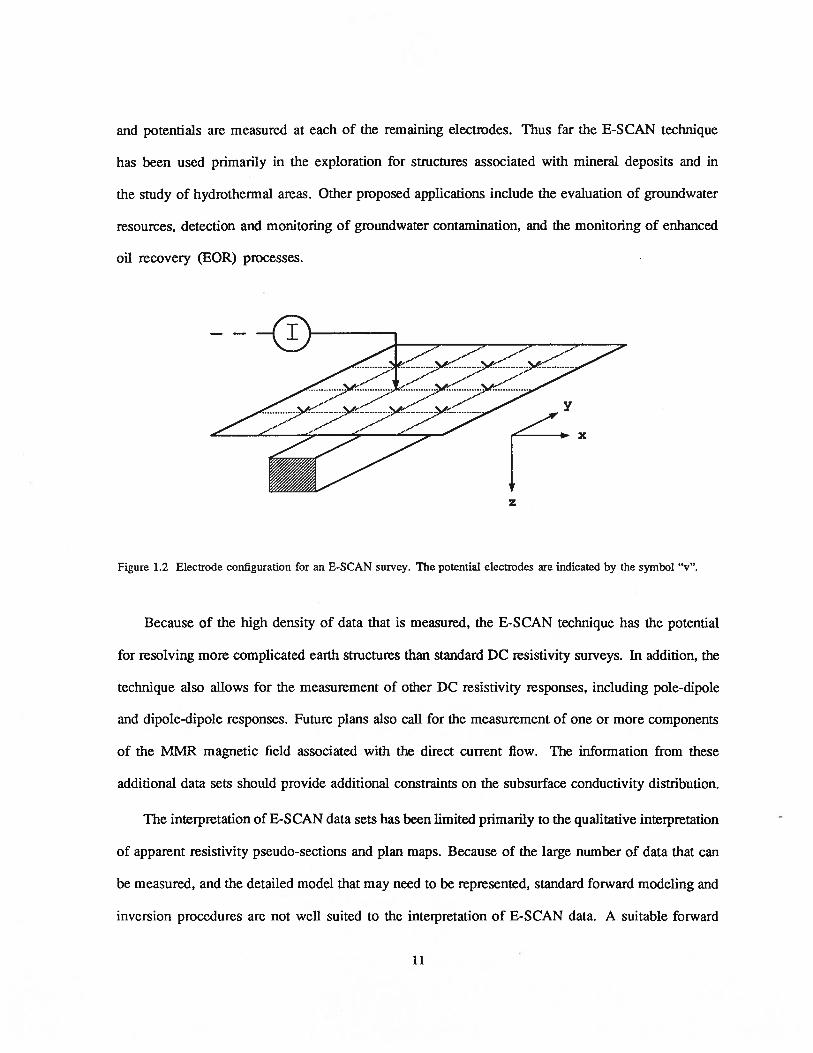
and potentials are measured at each of the remaining electrodes. Thus far the E-S CAN technique

has been used primarily in the exploration for structures associated with mineral deposits and in

the study of hydrothermal areas. Other proposed applications include the evaluation of groundwater

resources, detection and monitoring of groundwater contamination, and the monitoring of enhanced

oil recovery (EOR) processes.

Figure 1.2 Electrode configuration for an E-SCAN survey. The potential electrodes are indicated by the symbol “v”.

Because of the high density of data that is measured, the E-SCAN technique has the potential

for resolving more complicated earth structures than standard DC resistivity surveys. In addition, the

technique also allows for the measurement of other DC resistivity responses, including pole-dipole

and dipole-dipole responses. Future plans also call for the measurement of one or more components

of the MMR magnetic field associated with the direct current flow. The infonnation from these

additional data sets shonid provide additional constraints on the subsurface conductivity distribution.

The interpretation of E-SCAN data sets has been limited primarily to the qualitative interpretation

of apparent resistivity pseudo-sections and plan maps. Because of the large number of data that can

be measured, and the detailed model that may need to be represented, standard forward modeling and

inversion procedures are not well suited to the interpretation of E-SCAN data. A suitable forward

x

z

11

modeling algorithm must be able to accurately model a large and varied set of responses, including

pole-pole, pole-dipole, dipole-dipole data for either a line or a two-dimensional grid of electrodes.

A suitable inversion algorithm must be capable of inverting these large data sets, and have enough

flexibility to permit a very detailed representation of the subsurface. These requirements can make

the use of standard modeling and inversion procedures extremely expensive.

1.4 Solution of large-scale forward and inverse problems

To deal with the large-scale forward and inverse problems that are associated with B-SCAN,

MMR and conventional DC resistivity surveys, new, more efficient numerical procedures were needed.

1 4 1 Solution of the forward problem

The use of standard numerical techniques to model large-scale pole-pole resistivity and MMR data

sets is plagued by problems with accuracy and efficiency. Because of the large number of current

electrodes, and the complexity of the model that must be represented, the numerical grid used in

forward modeling can become very detailed. This can result in an excessively expensive calculation,

both in terms of computation time and memory requirements. In order to obtain a sufficiently accurate

solution without making the problem excessively expensive to solve, new approaches are needed. To

meet this need, the first phase of research was devoted to the development of accurate and efficient

forward modeling algorithms for the pole-pole resistivity and MMR forward problems.

In the initial stages of research a more traditional forward modeling algorithm, based on the

integrated finite difference technique, was developed. Particular emphasis was placed on accounting

for the errors that result from representing the continuous problem by a discrete problem. The method

of solving the discrete problem was selected so that the problem could be solved efficiently for a large

number of source locations. A secondary potential formulation for removing a singularity associated

with the current electrode was also incorporated into this basic algorithm. By properly removing the

12

singularity, considerable improvements in accuracy could be realized. The development and testing

of this finite difference algorithm is the focus of Chapter 2 of this thesis.

Because of the need to solve large problems, and to achieve the necessary resolution in the vicinity

of singularities, an iterative solution to the forward problem based on the multi-grid approach was

also developed. Rather than solving the numerical problem on a single grid, as is usually done, a

sequence of grids of increasing fineness is used. Since resolution is often required in only a small

region of the model near the electrodes, the grids in the sequence can also be made spatially less

extensive as they become finer. In this way the fine grids are used only to achieve accuracy in the

region of interest, while the coarser, more extensive grids are used to satisfy the boundary conditions

and to accelerate convergence of the fine grid solution. This can result in considerable computational

savings over more conventional approaches. As well, solutions are generated for grids of increasing

fineness, so that the numerical accuracy of the final solution can be assessed.

The application of the multi-grid algorithm to the solution of a particular problem requires a

careful choice of operators used in the multi-grid process. This is particularly critical in the DC

resistivity case, where discontinuities in the model and singularities in the solution can easily degrade

the convergence rate of the algorithm. Because of this, and the general complexity of the algorithm,

it has not been previously applied to geophysical problems of this nature. The development and

testing of a suitable multi-grid algorithm, and its use in the modeling of pole-pole resistivity data

are presented in Chapter 3.

Since the design of the numerical grid used in the solution of the forward problem results in a

trade-off between computational woiic and accuracy, it is important that the grid be properly designed.

If the grid is too coarse where the solution is changing rapidly, the accuracy of the numerical solution

will be poor. On the other hand, if the grid is too fine then the cost of the calculation will be

excessively high. Since the accuracy of the solution for a particular grid will depend on the model

and the survey geometry, it is difficult to design an adequate grid a priori. Based on the development

13

in Chapter 3, however, a study of the factors that control the accuracy of the solution can be helpful

in designing an adequate grid. These considerations led to the development of the adaptive grid

design procedure presented in Chapter 4. This approach requires solving the problem on a sequence

of grids, where each grid is obtained from a partial refinement of the previous grid in the sequence.

The refinement criterion is based on an analysis of the relative error between the solution on the

two finest grids. This approach can result in considerable computational savings since only those

regions of the model that contribute most to the error in the solution are finely discretized. An

adaptive multi-grid forward modeling algorithm that makes use of this strategy was developed for

the pole-pole DC resistivity problem. The development of this algorithm, and its use in the modeling

of pole-pole resistivity data, is presented in Chapter 4.

1.4.2 Calculation of sensitivities

In order to make the solution of 2D and 3D inverse problems tractable, the conductivity model

is usually parameterized by subdividing it into a number of sub-regions or blocks. The resistivities of

each block are then the parameters that are solved for in the inversion. Since the relationship between

the model parameters and the data is generally non-linear, an iterative solution to the inverse problem

is required. This involves improving, in an iterative manner, an initial estimate of the solution so

as to achieve a better fit to the observed data. These changes in the model can be related to the

desired improvement in the data by the sensitivities or partial derivatives of the data with respect

to the model parameters. Since sensitivities form the basis of most optimization procedures, their

calculation is fundamental to the solution of the inverse problem.

A variety of approaches exists for the numerical calculation of sensitivities. The approaches

differ, both in terms of the type of sensitivity information that is obtained, and in the computational

requirements of the algorithms. To assess these approaches, and to determine which was most suited

to the problem being addressed here, a detailed study of existing techniques was carried out. The

14

results of the study were used in the development of an efficient algorithm for the calculation of

sensitivities for the 2D pole-pole resistivity and MMR problem. The development and testing of this

algorithm is the focus of Chapter 5 of this thesis.

1.4.3 Solution of the inverse problem

Since only a finite number of data are available for characterizing what can be an arbitrarily

complicated earth, the inverse problem is inherently non-unique — there is generally an infinite

number of models that fit the observed data. In order to avoid problems with non-uniqueness, most

attempts at solving the inverse problem use a relatively coarse parameterization of the model. To

further reduce the non-uniqueness, the regional model is often specified a priori, and the resistivity of

only a small portion of the model is solved for in the inversion. Although these strategies can reduce

the mathematical non-uniqueness, other difficulties are likely to result from the loss of flexibility in

the solution. In particular, the outcome of the inversion will be strongly influenced by the form of the

parameterization and choice of regional model. The lack of flexibility in the solution can also lead to

poor convergence (or even divergence) of the model iterates, even if the form of the parameterization

is consistent with the true earth structure.

To avoid these problems the strategy adopted here is to make use of as fine a parameterization of

the model as possible. This gives the inversion algorithm maximum flexibility, and makes the outcome

of the inversion less sensitive to the way in which the parameterization is specified. Unfortunately,

this strategy can also result in a very significant increase in computational expense. Much of the

research presented here has focused on making the solution of these large-scale inverse problems

practical. In particular, an optimization procedure based on a generalized subspace formulation has

been developed. This reduces the number of effective parameters that must be solved for in the

inversion, while still maintaining the needed flexibility.

15

To deal with problems of non-uniqueness that arise when specifying a fine parameterization,

the solution to the inverse problem was required to have minimum structure relative to a specified

reference model. This was achieved by requiring that the model not only fit the observed data,

but also minimize an appropriate model objective function. Character that is not demanded by the

data is thus suppressed, leading to improved stability in the inversion. The use of this fonnulation

also allows one to take advantage of any a priori information about the true solution that might

be available. For example, the model norm can be chosen to emphasize certain features that are

anticipated in the solution.

The combined use of efficient forward modeling and optimization strategies, and the minimization

of a global norm of the model, leads to an inversion procedure that is both stable and computationally

practical. The development of an inversion procedure for large-scale problems is presented in Chapter

6. The use of this algorithm in inverting a variety of synthetic DC resistivity and MMR data sets,

and an E-SCAN field data set, is also presented.

16

Chapter 2

Finite Difference Solution of the 2D Pole-pole Resistivityand MMR Forward Problems

2.1 Introduction

Various algorithms have already been described for modeling resistivity data collected using

Schiumberger, dipole-dipole and other commonly used electrode arrays. These include algorithms

based on the finite difference, finite element and boundary element methods. In spite of the availability

of existing algorithms, none was found suitable for all of the problems that were considered in this

study.

A particular problem with existing forward modeling algorithms is the poor accuracy obtained

when modeling pole-pole responses. To obtain an accurate numerical solution it is first necessary to

understand where errors in the solution arise. This can be done through a study of the discretization

error that results from representing the differential operator by a discrete operator. The information

that this yields can then assist in the design of a more accurate numerical grid and can form the basis

of an adaptive approach to the solution of the forward problem. Although these are important

considerations in computing any numerical solution, they have received very little attention in

geophysics.

Second only in importance to accuracy, is the efficiency of the forward modeling algorithm. This

is particularly true if the algorithm is to be used in the solution of the inverse problem, where many

forward solutions may be required to obtain a model that fits the data. Two ways of maximizing the

17

efficiency of the forward modeling algorithm can be considercd. The first is to keep the numerical

grid as coarse as possible without degrading accuracy. An algorithm that can be made more accurate

will thus also be more efficient. The second approach is to consider alternate numerical formulations

that are inherently more efficient. The need for more efficient procedures led to the investigation of

the multi-grid and multi-level approaches presented in Chapter 3.

Because of the desire to examine a wide variety of problems, it was important to develop an

algorithm with as much flexibility as possible. Of particular importance was having the flexibility

to model a variety of different responses, including pole-pole, pole-dipole, dipole-dipole and MMR

measurements for surface, cross-borehole and borehole-to-surface arrays. The flexibility to consider

complex conductivity structures and to include topography was also considered essential. As discussed

in Chapter 5, the sensitivities, which are at the heart of most inversion routines, can be computed

using the same forward code used to compute the forward responses. The forward modeling algorithm

must thus be able to model a large number of sensitivities accurately and efficiently if the solution

to the inverse problem is to be practical.

To meet the needs of this research, a forward modeling algorithm based on the integrated finite-

difference formulation was developed. The basic algorithm was then used in the formulation of

more efficient multi-level and adaptive multi-grid solvers described in Chapters 3 and 4, and was

also incorporated into the generalized sub-space inversion algorithm presented in Chapter 6. The

development and testing of the algorithm is the focus of this chapter.

2.2 Mathematical formulation

The first step in obtaining a numerical solution to any forward problem is to derive the governing

equation and boundary conditions that describe the physical experiment. For the DC resistivity

experiment these are developed from basic physical principles, beginning with the expression for

18

conservation of charge

(2.1)

where J is the current density and I is the current injected into the ground at = (x3,y3,z3).

Ohm’s law for a 2D conductivity model u(x, z) can be written as

1= —u(x,z) (2.2)

where (x, y, z) is the scalar potential. The governing differential equation for the DC resistivity

problem, obtained by combining (2.1) and (2.2), is then found to be

= —. (c(x,z)’c) = 15(x— Xs)’5(y — ys)(z — z3) (2.3)

For a horizontal air-earth interface the potential must also satisfy the boundary conditions

(9(2.4)

and

= 0 (2.5)

where R = — x)2 + (y — y5)2 + (z—z3)2. Topography can be included in the problem by

assigning small values of conductivity to regions above the air-earth interface.

2.2.1 Transformed problem

Although a two-dimensional conductivity structure has been assumed in this work, the potential

field that results from injecting current into the ground at a single point current electrode is still

three-dimensional. The effective dimensionality of the problem can be reduced by considering the

Fourier cosine transform of the total potential, given by

= (x,k,z) = J(xyz)cos(kvy)dy (2.6)

19

where k is a spatial wavenumber in the y direction. (e.g. Snyder 1976, Dey and Morrison 1979a,

Gomez-Trevino and Edwards 1979, Mundry 1984). The transformed potential is then found to

satisfy the boundary value problem

= _—o(x, z) + k(x, z) — -cr(x, z).i = — x)ö(z — z) (2.7)

= 0 (2.8)

0 (2.9)

where r8 = — x3)2 + (z — z)2. The factor of on the right hand side of (2.7) arises because

the limits of the integral transform in (2.6) are from zero to infinity and the problem is symmetric

about the y axis.

If (2.7-2.9) is solved for a series of wavenumbers, then the potential in the spatial domain can

be obtained by numerically evaluating the inverse Fourier cosine transform

ó(xy,z) = f(x,k,z)cos(ky)dkv (2.10)

The full 3D problem is thus reduced to a more tractable set of uncoupled 2D problems.

2.3 Discretization of the forward problem

Except when dealing with very simple models one must usually resort to numerical methods to

obtain a solution to (2.3-2.5) or (2.7-2.9). Recent work on the numerical solution of the DC resistivity

forward problem has concentrated on the use of the finite element method (Coggon 1971, Rijo 1977,

Pridmore et aL 1981, Fox et al. 1980, Holcombe et al. 1984), finite difference method (Mufti 1976,

Dey and Morrison 1979a,b, Mundry 1984, James 1985, Lowry et al. 1989) and boundary element

method (Snyder 1976, Oppliger 1984). A variation on the solution of the finite difference method

for the 2D pole-pole problem is presented below.

20

— a(x,z) dl+kf u(x,z)dA

=

I(x — x)S(z — z3) dA

2

SI SI -

:1z___Figure 2.1 Two dimensional finite difference grid used to discretize the transformed DC resistivity problem. The

current electrode is indicated by an arrow, the potential electrodes by V’s.

2.3.1 Discretization to obtain the FD operator and truncation error

The first step in formulating the numerical problem is to develop a discrete approximation to (2.7).

Given a 2D earth model, a rectangular grid is first superimposed over the model and conductivity

values are assigned to each element in the grid, as shown in Figures 2.1 and 2.2.

For the ij internal node, the governing equation (2.7) is integrated over the corresponding cell

(shaded in Figure 2.2), yielding

(2.11)

z

21

The two terms on the left side of (2.11) are expanded as

z+Iz/2

—

dl= —f

+x1/2,z) dz

+f

-(x,zj +zj/2) dx +f 1-(x,zj +izj/2) dx

(2.12)

— f — x_i/2,z) dz —

z,+4z, /2

— fui(x + x/2,z) dz

z—zz1_1/2

iji—1

j —1

4,, ::

_______

—

1+1]Z

•1•1

ijk-1

Ax_1 L\x

Figure 2.2 Finite difference operator used in the discretization of the transformed DC resistivityproblem. The shaded region corresponds to the ij cell.

22

andr.+.x,/2 z+1z,/2

k fci(x, z) dA = kf Ju.i(x, z) dx dz

+k J J.iics(x,z)dxdz + ... (2.13)

—x_1/2 Zj

x,+ix,/2 z,

+kf Ja1(x, z) dx dx

X,z,—z,_i /2

Taylor series expansions are then used to relate the integrands to the values of the potential at

the ij and adjacent nodes. For example -

+ x/2,z) = + (a)+1+(z — z)

— + (ux)xzI,++ x(z — z)

——

(2.14)

+(x)xxzI+i+(Xi)2(Z— zj) + x)zzI,+j+xi(z —

— zj)3 + 0(h4)

andc(x,z) = + (a)I+,+(x — x) + (a)I÷+(z — z)

— x)2 + ()zI,+1+(x — x)(z — zj) (2.15)

— z)2 + 0(h3)

where h = and 0(h’) is a term that approaches zero as quickly as

h as h —÷ 0. Limits in the expansions, for example

(c) j++ = lim (2.16)

are assumed to exist.

Carrying out the integrations in (2.12) and (2.13), and combining terms, yields the five-point

finite difference operator

a1,_1+b1_1 + + + = Li + (2.17)

23

wherec7_1_1LZ_1+ o-,_13z1

a,, =— 2x1_,

b— + °j_L’

2Lz,_,

k2c,, = —(a,, + b,, + d,, + e,,) + - (o1t.x4z +_1,x,_1z,

+ cr_1x4z,.1+o1_11_1x,_1z_1) (2.18)

d —

— + c7,,zx,‘2

— 2z

—— o.ij_1zj_1+

— 2x

and f,, the integrated source term, is given by

= f 6(x — x8)6(z — z)dx dz = for electrode at ij’th node2 D,, 2 (2.19)

= 0 otherwise

The truncation error, is given by

= z,.(x2(u)I+ —

+ 48(.3(cb)I + x(crcb)I,-)

+‘ +x,_i

(z()+ —(2.20)

+‘ ‘‘

(z(u&),+

+ 0(h5)

For a continuous model and uniform grid the first term in (2.20) vanishes, leading to an 0(h2)

approximation. Otherwise, the approximation is 0(h). Since the order of the approximation

approaches zero as h —f 0, the scheme is said to be consistent. Consistency guarantees that for

a stable problem (i.e. one for which a unique solution exists) the numerical solution will converge

to the exact solution as the grid spacing is reduced.

24

2.3.2 Approximation of boundary conditions

Finite difference equations for nodes along the upper boundary of the grid are derived in the

same way, with the boundary condition (2.8) being applied prior to integration. Nodes along the

left, right, and lower boundaries require special attention since the infinity boundary condition (2.9)

cannot be used on a finite grid. To describe the solution along one of these boundaries, the mixed

boundary condition

k, z) + a(x, k, z) 0 (2.21)

is used (Dey and Morrison 1979a,b). This has the advantage of specifying the form of the solution

without restricting its amplitude. The coefficient a is determined from the asymptotic behavior of the

potential away from the source region. Using this approach, the true source distribution (including

secondary sources) is represented by a point source located at or below the center of the electrode

array. For a point source in a halfspace of conductivity a1!2’ the asymptotic transformed potential

is given by

.K0(k) (2.22)2ira112

where r3 = — x)2 + (z — z3)2. The appropriate value for a at a particular boundary node is

then obtained by substituting the analytic solution for the point source into (2.21), yielding

K1(kyr.) aa = 1c , —r (2.23)

IkO(kyr.) an

For this asymptotic representation to be accurate the boundaries must be far enough from the

anomalous region that the source distribution can in fact be represented by a single point source.

The accuracy of the representation is poorer for small wavenumber components of the solution,

which have energy out to greater distances from the electrode. This limits the value of the smallest

wavenumber that can be accurately modeled on a particular grid.

25

The finite difference approximations for boundary nodes arc found to be of the same form as

(2.17-2.19). Expressions for the truncation error show that the approximations are again 0(h2) for a

smoothly varying model and uniform grid spacing, and 0(h) otherwise.

2.3.3 Assembly of the matrix system

Having obtained discrete representations for the governing equation and boundary conditions at

each node, the transformed forward problem can be written as the system of linear equations

Lçb = f (2.24)

where 1, is the sparse, banded matrix whose entries are the finite difference coefficients for each node.

2.4 Singularity removal

The singular nature of the source term in (2 3) can present difficulties when the potentials are

solved for directly. Note that close to the current electrode the potential will approach the halfspace

response

(x,y,z)=

___

12 2

(2.25)2ircr0 r-+(y-y) +(z-z)

where o is the conductivity around the current electrode. Taking the Fourier cosine transform of

the halfspace response yields

K(kyr.) (2.26)2iru0

which displays a logarithmic singularity as r5 = /(x — x3)2 + (z— z)2 — 0.

One method for treating the singularity is to refine the mesh in the area around the singularity.

This approach is most practical when used in a multi-grid formulation, where the refinement can be

done without an overwhelming increase in cost. For numerical modeling algorithms that construct

the solution from a set of basis functions (i.e. the finite element or boundary element methods) one

can augment the set with higher order basis functions (Cavendish et al. 1969). These higher order

26

functions are chosen so that the solution can be represented more accurately near the singularity.

Another possibility is to make use of a local solution defined on an “analytic patch” containing the

singularity (Cavendish et al. 1969, Hayes et al. 1977, Charbeneau and Street 1979a,b). The local

solution represents the singularity exactly, so that the total solution less the local analytic solution

can be more accurately modeled.

2.4.1 Modeling of secondary potentials

The approach used in this work involves reformulating the problem so that only the secondary

response is modeled. (The secondary response is defined as the total response less some analytic

reference or primary response that includes the singularity.) Coggon (1971) and Rijo (1977) apply this

technique to the modeling of EM and DC resistivity responses using the finite element method. Pelton

et al. (1978) discuss some of the advantages and disadvantages of modeling anomalous potentials for

the DC resistivity problem. Lowry et al. (1989) model anomalous potentials for various electrode

arrays using an integral finite difference scheme. Although the modeling of secondary responses is not

new, the way in which the secondary problem has been formulated in the past can lead to poor results

for certain kinds of models. An improved solution for the secondary responses is described below.

To deal with the singularity associated with the 2D pole-pole resistivity problem, a primary po

tential (x, k, z) and a secondary potential 5(x, k, z) are first defined. The reference conductivity

structure can be a halfspace, or any other model for which transformed potentials can be computed

analytically (i.e. a dike, vertical contact or layered halfspace), and is chosen so that the secondary

response is small relative to the primary response. Let u,,(x, z) and u3(x, z) = a(x, z)—

o(x, z)

denote the reference and anomalous conductivity respectively. Substituting for q. = + cb in (2.7)

and noting that

44 = —

z) + ka(x, z)4—

u(x,z) = — — z) (2.27)

27

leads to the governing equation for the secondary potentials

ic= __cr(x,z)-. + ka(x,z)5—o.(x,z)-i

=—

(2.28)

where

_(L—4)p=-as(x,z) —ku(x,z) +_(x,z)2 (2.29)

Note that the point source representing the current electrode in the original problem has been replaced

in the secondary problem by a current density distributed throughout the domain. The boundary

conditions for the secondary problem are

0-= 0 (2.30)

and

= 0 (2.31)

Together, (2.28-2.31) constitute the boundary value problem that must be solved to obtain the

secondary potentials.

2.4.2 Discretization of secondary potential problem

Applying the finite difference discretization scheme described earlier to the secondary problem

(2.28-2.31) yields the system of linear equations

= .f (2.32)

where the coefficient matrix L is the same as that used in solving for the total potentials, and

f8 is a discrete approximation to the secondary source term. Care must be taken in obtaining an

accurate representation of the source term for the secondary problem. Previous efforts at solving for

secondary potentials have made use of the same finite difference operator to discretize both sides of

the governing equation. Thus the discrete problem

=—

(I—

L) (2.33)

28

is solved, where L is the coefficient matrix that results from discretizing the primary potential

problem and is the continuous primary potential sampled at each node in the grid. Although

this discretization appears reasonable, it can lead to large errors in the computed solution, particularly

when the current electrode is buried in a region that is conductive relative to other regions in the

model.

To show why (2.33) is not an appropriate representation for the secondary source term, the

truncation error for the discretization must be examined. Note that the exact solution to the continuous

total potential problem, cont’ satisfies

= f + f (2.34)

where is the truncation error. As well

= f + (2.35)

Combining (2.34) and (2.35) yields

s,con =—

(L—

L) p,cont + —(2.36)

The truncation error that results from using the discretization in (2.33) is thus

=—(2.37)

29

Medium 1 Medium 2

Figure 2.3 Quarterspace problem used to illustrate the accuracy problems associated with the

discretization scheme given by (2.33)

To illustrate the result of using the discretization in (2.33), the quarterspace problem shown in

Figure 2.3 was considered. Substituting the analytic solution for the secondary potential into (2.20),

yields expressions for the truncation error f in each medium. These are

(x,k,z) = r12 (4 + — b)2 +Y2) . (2.38)

in medium 1, and

f3(x,k,z) = r21-• (-- + — b)2 + y2) (2.39)

in medium 2, where r12 = = —r1, and = zj = for all i and j. If o-i >> u2 then

the resulting error contributed to the solution in medium 1 is proportional to i/o-i and the relative

error is independent of the conductivity in either medium. In medium 2, the error is proportional

to i/a2 so that the relative error is proportional to o-i/o-2. Clearly for the case of cr >> CT2, the

discretization scheme in (2.33) will lead to large errors in the more resistive quarterspace.

A more accurate representation of the secondary source term can be obtained using the dis

cretization

= fs,int + tnt (2.40)

30

where frjj is obtained by integrating the analytic secondary source distribution over each cell in

the grid. For the cell in Figure 2.2 this yields

= —f (—4)dxdz

= fD,( Ox Ox— kcT8 + s)dxdz (2.41)

1 (+--cixdzOx 9z OzJ

Since the model is assumed to consist of a set of homogeneous blocks, the derivatives of the

conductivity in (2.41) can be written as

Oo— J’ (u2j — c_1)6(x — x) for z> zj

— 1 (u — a_ii)6(x — x) for z < Z

(2.42)

Oos— f (oj — — z) for x > x

— 1 (i_i — z1) for x < x

Equation (2.41) then becomes

(!s,int)ii = — a_1) J+ (u_1

—) f(2.43)

+(ij_1j) f (x1,k,z)dz

+ (_ —u) f k, z) dz

z1—z3_1/2

A five-point Gaussian quadrature scheme was used to evaluate each of the integrals in (2.43). Since

this results in a very accurate integration, the error in discretizing the source term is essentially zero.

Since all of the source is accounted for in (2.40), the scheme is said to be conservative. Clearly this

will not be the case with the discretization in (2.33) since — (L — L) c, will be non-zero wherever

the conductivity differs from that at the current electrode.

31

An analysis of the truncation error for the quarterspace problem can also be carried out for

the discretization scheme in (2.40). The relative error in both quarterspaces is then found to be

independent of the conductivities.

To illustrate the impact of using a non-conservative discretization, secondary potentials were

computed for the vertical contact model in Figure 2.3. In the first case the left quarterspace, which

contained the electrode, had a resistivity of 10.0 m and the right quarterspace had a resistivity of

1000.0 fm. For the second case the resistivities of the two quarterspace were interchanged. The

secondary potentials for y = 100.0 m obtained using the two discretization schemes are compared

to the analytic solutions for the two models in Figure 2.4. As expected, a severe error is observed

in the solution corresponding to the non-conservative scheme when the electrode is buried in the

more conductive quarterspace. When the resistivities are interchanged, the discretizations are found

to yield comparible results. Although this analysis was carried out for a simple model it is clear

that similar problems will be encountered for the non-conservative scheme whenever the current

electrode is placed in a locally conductive region.

0.08

0.06

0

0.02

0.00—800 —400 0 400 800 —800 —400 0 400 800

X position (m) X position (m)

Figure 2.4 Secondary potentials computed using the conservative discretization scheme (triangles) and non-conservative

scheme (dashed line) compared to the analytic solution (solid line) for the model in Figure 2.3 with (a)

= [0.0 Qm and P2 1000.0 m, and (b) with P’ = 1000.0 Qm and P2 = 10.0 f2m. For both

problems, a current of 10 A was injected at the surface of medium 1 at x = —67.0 m and the

potentials were modeled for y = 100.0 m. The contact was located at x = 67.0 m.

>

0

C0

0a-

32

2.5 Method of solving the discrete matrix equations

For the solution of matrix problems the matrix problems in (2.24) and (2.32), a direct solver based

on the Cholesky decomposition (Golub and Van Loan 1983) was used. For the general problem

Aii= (2.44)

the Cholesky decomposition involves factoring the coefficient matrix A into a lower and an upper

triangular matrix

A = LLT (2.45)

where L and LT are respectively lower and upper triangular matrices. The system in (2.44) becomes

LLTi = b (2.46)

Letting

LTII = (2.47)

the vector can be computed by solving

(2.48)

by forward substitution; the solution ñ is then obtained by solving (2.47) by backward substitution.

Although the Cholesky factorization can be expensive, obtaining solutions for different right

hand sides is relatively economical once the factors have been computed. This is an important

consideration in the DC resistivity forward problem, where each current electrode in the physical

problem corresponds to a different right hand side that must be solved for in the numerical problem.

As well, if the inverse problem is also to be addressed, the sensitivities must also be forward modeled.

This involves solving the original forward problem repeatedly for sources located at each observation

location. Because of the need to solve for a large number of right hand sides in the DC resistivity

problem, the Cholesky factorization was considered a practical choice.

33

2.6 Inversion of the Fourier transform

Once the transformed forward problem has been solved for a set of wavenumbers, the potentials

in the spatial domain are obtained by numerically evaluating the inverse transform given in (2.10).

For pole-pole calculations this step is of extreme importance since errors associated with inverting

the transform are not cancelled by taking differences, as they are when responses for dipole current or

potential electrodes are modeled. In this regard, the low frequency part of the integration is critical.

As pointed out by Pelton et al. (1978), the use of a simple quadrature scheme to evaluate

the inverse transform can lead to poor results if the spectrum is not a monotonically decreasing

function. This is a particular problem when integrating transformed secondary potentials since the

associated spectrum often display a great deal of character. A more accurate solution is obtained by

using a cubic spline to interpolate between modeled points in the spectrum. This is done in the log

wavenumber domain since the spectrum is expected to change rapidly near = 0 and less rapidly

for large k. Once the spline has been fit to the modeled potentials, a high density of interpolated

points are generated. Four or five interpolated potentials between each pair of modeled potentials

are usually sufficient to accurately represent the spectrum. A piecewise linear function is fit to the

interpolated spectrum and the integration is then carried out analytically. The resulting quadrature

formula is given by

f(y) = Jf(x)cos(xy)dx

2(ax+bjcos(xy)dx (2.49)

7r

(a,C0 +j(x)s)

where

= f(x,) f(x)

-x,+1 —

(2.50)— —

xf(x1)

34

In the solution of the 2D pole-pole inverse problem, it is often necessary to integrate a large

number of transformed sensitivities for each iteration. Since accuracy is less important in the

calculation of the sensitivities, the use of the integration scheme described above is not necessary.

Instead of using a spline to generate a denser sampling of the spectrum, a piecewise exponential

function is fit to the modeled data and the integration is carried out analytically using

f(y) = JJ(x)cos(xy)dx

2 f be cos (xy)dx (2.51)

j xi

2V-\j( )a3sin(XY) ycos(xy) X+i

a+y2

where

a.=’’’xi+1 —

- (2.52)

= expx+1lnf — xlnf+,

xi+1 —

This is the same approach used by Dey and Morrison (1979a), and others.

The accuracy of the integration depends on how well the spectrum is initially sampled. Best

results have been obtained by sampling the spectrum for ten or more approximately logarithmically

spaced wavenumbers. When selecting the range of wavenumbers to be sampled it is important to

consider whether one needs to calculate potentials for non-zero values of y, in which case more care

must be taken in sampling the low frequency portion of the spectrum. Although these are useful rules,

they are very approximate. Generally it is worthwhile to examine spectra of the modeled potentials

for selected locations to insure proper sampling.

2.7 Examples

To demonstrate the accuracy of the integrated finite difference algorithm, total and secondary

potentials were modeled for a series of example problems. For consistency, the grid depicted in

35

Figure 2.5 was used in all of the forward modeling calculations. A detail of the center portion of the

grid below the area of interest is shown in Figure 2.6. A standard suite of 16 wavenumbers (0.000 1,

0.000325, 0.0005, 0.001, 0.0025, 0.00325, 0.005, 0.01, 0.025, 0.05, 0.1, 0.3, 0.7, 1.0, 5.0, 10.0)

was used in all of the examples.

As a test of the overall accuracy of the finite difference algorithm, transfonned potentials were

first modeled for the quarterspace problem shown in Figure 2.7. A current of 10 A was injected

into the ground at = (—67.0,0,0) m. The transfonned total and secondary potentials modeled

for a potential electrode at = (0, 100,0) m are shown as solid lines in Figures 2.8a and 2.8b

respectively. The same results are shown for a potential electrode at CF,, = (167, 100, 0) m in Figures

2.8c and 2.8d. The numerically computed transformed potentials, indicated by triangles, are in good

agreement with the analytic solutions, which are indicated by solid lines. For both total and secondary

potentials the spectrum varies exponentially over most of the range of sampled wavenumbers and

an exponential interpolation would be expected to perform well. Using the inverse Fourier cosine

transform algorithm described earlier, the potential profiles in Figure 2.8e and 2.8f were obtained.

As expected, these results are also in good agreement with the analytic solutions. Only at the node

0.0

______

r:4-

E

4J0-.a)0

4000.0

—4000.0 0.0 4000.0

Distance (m)

Figure 2.5 Finite difference grid used to solve the transformed resistivity problem.

36

corresponding to the current electrode at x = —67 m, for the total potential result in Figure 2.8e,

does the error become large.

0.0 — — —

C

4J

G)

1000.0

—1000.0

zz:z:0.0

Distance (m)

1000.0

Figure 2.6 Detail of the finite difference grid in Figure 2.5.

0.0

C

6)

0.0

Distance (m)

Figure 2.7 Quarterspace model used to test the results of the finite difference algorithm. The resistivities of theleft and right quarterspaces are 10 fm and 1000 flm respectively and the contact is at x = 67 m. Acurrent of 10 A was injected into the ground at i = (—67.0,0,0) m.

EHHHHE1000.0

—1000. 0 1000.0

37

1 40

E>

100Ca)00

•0a)

E0

C0

120

80

60

40

20

0

io-

120

100

80

° 600

40

20F-

0

iO-

0.20

0.15

0

0.100a-

0.05

0.00

101

101

E>

0

Ca)00

-oa)E0

C0

F—

io— io— 10—2 101 10° 101

Wavenumber (rn—1)

60

50

0

Ca)0a.

-oa)20U,C0

I—

40

30

20

10

N

0

0.08

-: 0.06

0

0.04

0.02

r, nra

iO- 10—2 10—1 10°

Wovenumber (rn—1)

d.

101

—800 —400 0 400X position (m)

800

Figure 2.8 Forward modeled results for the quarterspace model in Figure 2.7. (a) Transformed total potentials for

(0, 100, 0) m. (b) Transformed secondary potentials for i (0, 100, 0) m. (c) Transformed total

potentials for = (167, 100, 0) m. (d) Transformed secondary potentials for i = (167, 100, 0) m. (e) Total

potentials computed by numerically evaluating the inverse Fourier cosine transform. (f) Secondary potentials.

The numerically computed quantities are shown as triangles, the analytic solutions as solid lines.

iO— 10—2 10’ 10°Wovenumber (m’)

10—i 102 1O— 100

Wovenumber (m1)

—800 —400 0 400 800

X position (m)

38

As a second test, transformed potentials were modeled for the vertical dike problem shown in

Figure 2.9. The transformed total and secondary potentials at I, = (0, 100,0) m are compared to the

corresponding analytic solutions in Figures 2.lOa and 2.lOb. The numerically computed transformed

potentials are again in good agreement with the analytic solutions.

0.0

———————f——— -

EZZ]1000.0

—1000 .0

Figure 2.9 Vertical dike model used to test the results of the finite difference algorithm. The resistivities of the left andright quarterspaces are 10 Qm and 100 m respectively. The resistivity of the dike is 1000 2m.

4)

a)

0.0

Distance Cm)

1000.0

39

>

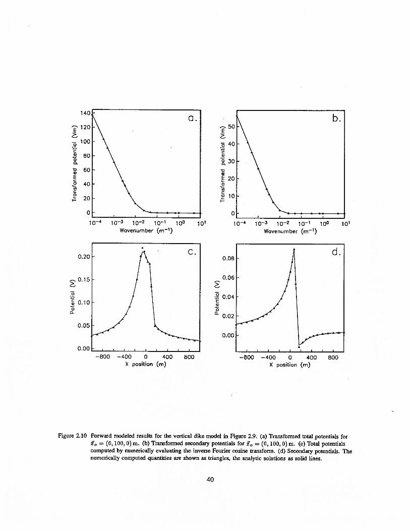
0

C0

00

>

0

C0

00

io— 10—2 10—1 100 10’Wavenumber (m1)

Figure 2.10 Forward modeled results for the vertical dike model in Figure 2.9. (a) Transformed total potentials for= (0, 100, 0) m. (b) Transformed secondary potentials for i = (0, 100, 0) m. (c) Total potentials

computed by numerically evaluating the inverse Fourier cosine transform. (d) Secondary potentials. Thenumerically computed quantities are shown as triangles, the analytic solutions as solid lines.

140

120>

100

C

.i 8000.

60E.2 40

20

b.

io0

iO- io— 10—2 10 100

Wovenumber (m’)

101

—800 —400 0 400X position (m)

800 —800 —400 0 400X position (m)

800

40

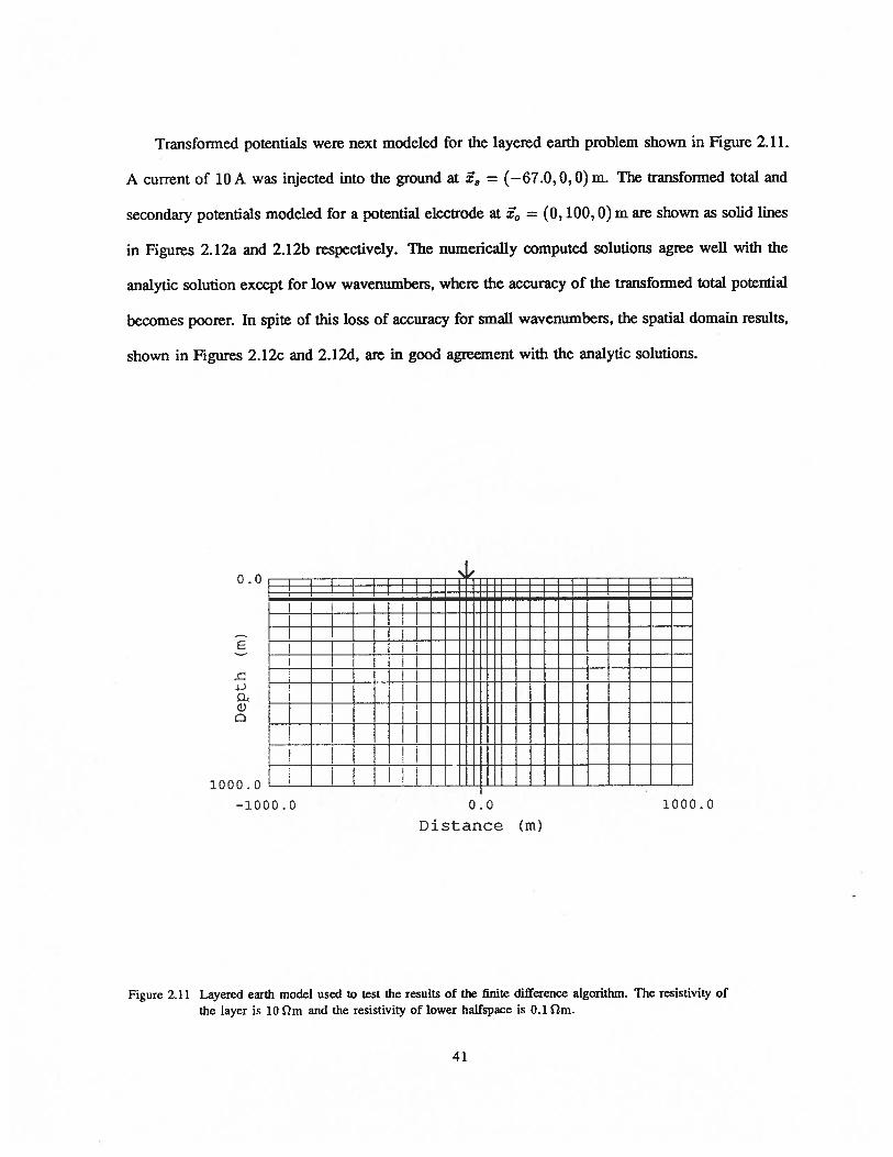
Transformed potentials were next modeled for the layered earth problem shown in Figure 2.11.

A current of 1OA was injected into the ground at = (—67.0, 0, 0) m. The transformed total and

secondary potentials modeled for a potential electrode at , = (0, 100,0) m are shown as solid lines

in Figures 2.12a and 2.12b respectively. The numerically computed solutions agree well with the

analytic solution except for low wavenumbers, where the accuracy of the transformed total potential

becomes poorer. In spite of this loss of accuracy for small wavenumbers, the spatial domain results,

shown in Figures 2.12c and 2.12d, are in good agreement with the analytic solutions.

E

-1J

0)

Figure 2.11 Layered earth model used to test the results of the finite difference algorithm. The resistivity of

the layer is 10 !m and the resistivity of lower halfspace is 0.1 !lm.

0.0

::z:::

I

z:z:rzz:]Dz::1000.0

—1000.0 0.0Distance (m)

1000.0

41

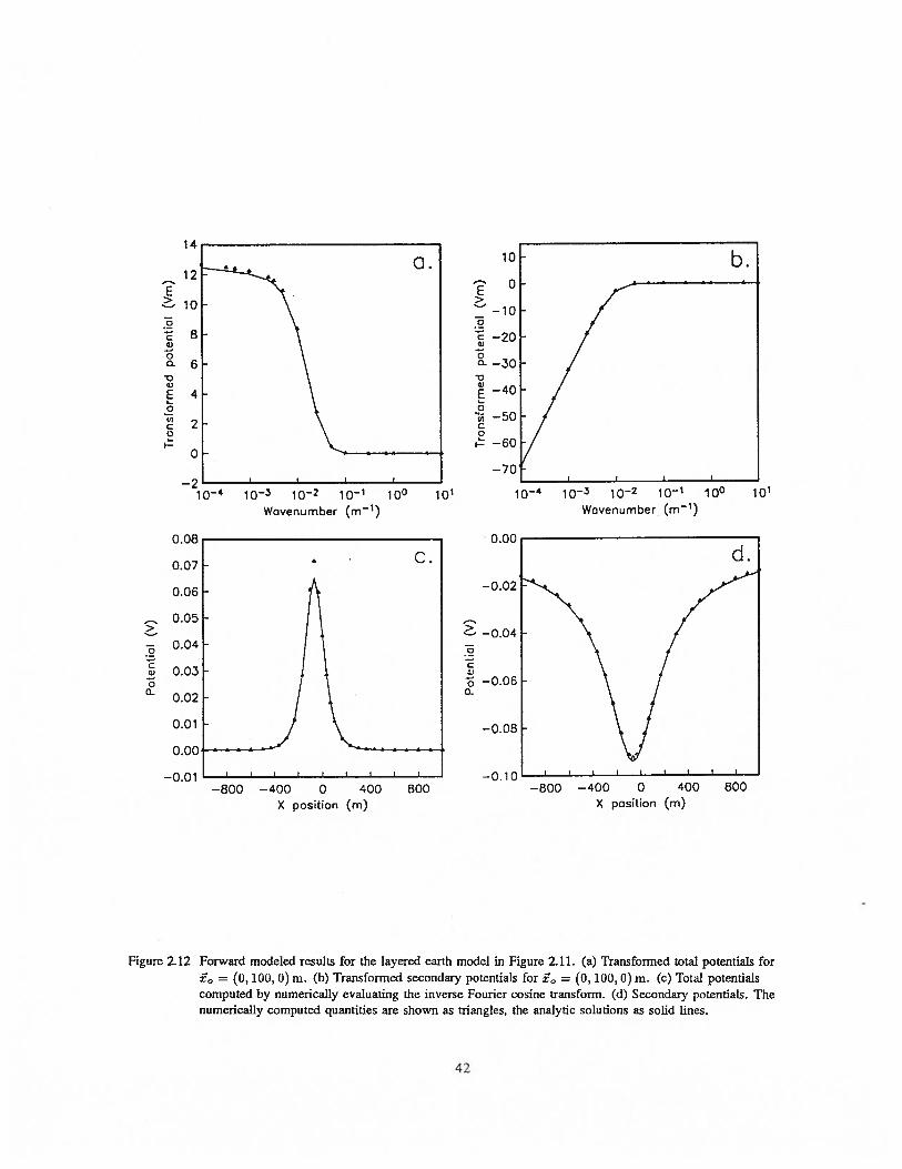
IA

Figure 2.12 Forward modeled results for the layered earth model in Figure 2.11. (a) Transformed total potentials for= (0, 100, 0) m. (b) Transformed secondary potentials for = (0, 100, 0) m. (c) Total potentials

computed by numerically evaluating the inverse Fourier cosine transform. (d) Secondary potentials. Thenumerically computed quantities are shown as triangles, the analytic solutions as solid lines.

E>

0

C

00.

5,

E05C0

I—

12

10

8

6

4

2

0

6>

0

C5)

0a.•05,60aCC

I-

10

0

—10

—20

—30

—40

—50

—60

—70— —

io- 10—s 10—2 10 100 101

Wovenumber (m)

io— 10—2 10—1 10°Wovenumber (m’)

101

>

0

C5)

0a-

>

C

Ca)0

a-

—800 —400 0 400 800X position (m)

—800 —400 0 400

X position (m)800

42

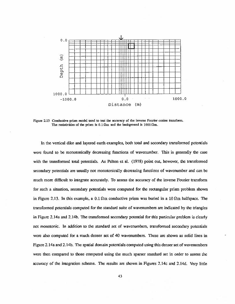
0.0

1000.0

—1000.0 0.0 1000.0

Distance (m)

Figure 2.13 Conductive prism model used to test the accuracy of the inverse Fourier cosine transform.The resistivities of the prism is 0.1 fm and the background is 1000 2m.

In the vertical dike and layered earth examples, both total and secondary transformed potentials

were found to be monotonically decreasing functions of wavenumber. This is generally the case

with the transformed total potentials. As Pelton et al. (1978) point out, however, the transformed

secondary potentials are usually not monotonically decreasing functions of wavenumber and can be

much more difficult to integrate accurately. To assess the accuracy of the inverse Fourier transform

for such a situation, secondary potentials were computed for the rectangular prism problem shown

in Figure 2.13. In this example, a 0.1 2m conductive prism was buried in a 10 Qm halfspace. The

transformed potentials computed for the standard suite of wavenumbers are indicated by the triangles

in Figure 2. 14a and 2. 14b. The transformed secondary potential for this particular problem is clearly

not monotonic. In addition to the standard set of wavenumbers, transformed secondary potentials

were also computed for a much denser set of 40 wavenumbers. These are shown as solid lines in

Figure 2. 14a and 2. 14b. The spatial domain potentials computed using this denser set of wavenumbers

were then compared to those computed using the much sparser standard set in order to assess the

accuracy of the integration scheme. The results are shown in Figures 2.14c and 2.14d. Very little

43

E>

a

V

00

E0

C0

Figure 2.14 Forward modeled results for the conductive prism model in Figure 2.13. (a) Transformed total potentials for= (0, 100, 0) m. The triangles indicate the coarsely sampled spectrum (16 wavenumbers),

the solid line indicates the more finely sampled spectrum (40 wavenumbers). (b) Transformedsecondary potentials for = (0, 100, 0) m. (c) Total potentials computed by numericallyevaluating the inverse Fourier cosine transform using 16 and 40 wavenumbers, shown as trianglesand solid lines respectively. (d) Secondary potentials computed by numerically evaluatingthe inverse Fourier cosine transform using the two sets of wavenumbers.

difference is seen between the results computed with the different sets of wavenumbers, indicating

an accurate integration.

80

>

600

5000.4Q0VE 300

20CC- 10

0

io-

0.14

0.12

iO 10—2 10—1 100 101

Wavenumber (rn—1)iO— 10—2 10—1

Wavenumber (m1)

._.. 0.10>

0.08CV

0.06a-

0.04

0.02

0.00

>

0

CV

00.

—800 —400 0 400 800 —800 —400 0 400 800X position (m) x position (m)

44

2.8 Modeling of topographic responses

Because electrical surveys are seldom canied out over flat terrain it is important to be able

to include topography into any forward modeling problem. Modeling the effects of topography is

relatively straightforward with the boundary element and finite element methods, where irregular

boundaries can be easily generated. The nature of the finite difference4method makes it more

difficult to represent irregular boundaries. A simple solution is to approximate regions of air around

topographic highs by elements having small but non-zero conductivities. In this way a rectangular

grid can still be used to represent the domain.

To verify this approximation is accurate, the finite difference algorithm was used to model the

terrain effect due to the “cliff’ shown in Figure 2.15. For the numerical computations a resistivity

0.0

E

41

0)

1000.0

—1000.0 1000.0

Figure 2.15 Cliff model used to illustrate the calculation of terrain effects using the finite differencealgorithm. The resistivity of the left quarter space prism is 10 fm. To simulate a region ofair, the right quarterspace was assigned a resistivity of 1.0 x irn.

0.0

Distance (m)

45

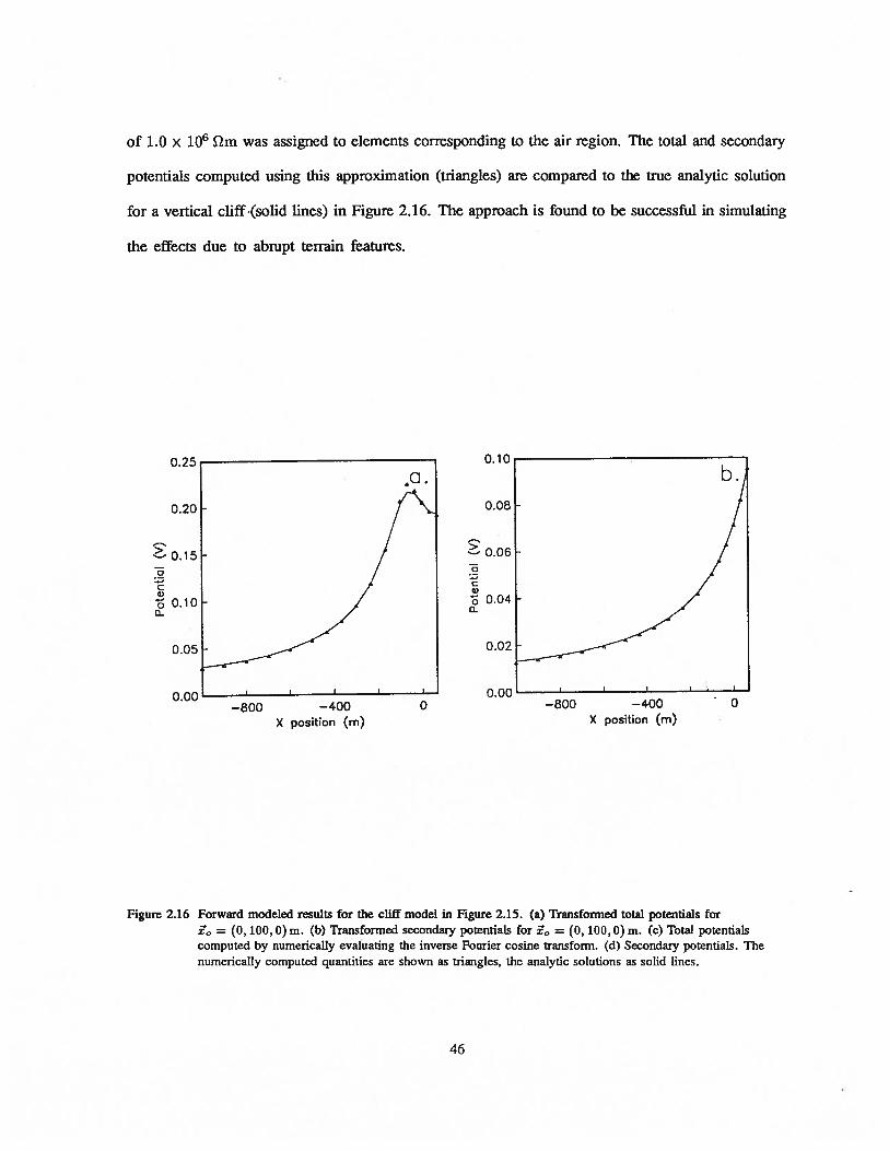
Figure 2.16 Forward modeled results for the cliff model in Figure 2.15. (a) Transformed total potentials for= (0, 100, 0) m. (b) Transformed secondary potentials for £,, = (0, 100,0) m. (c) Total potentials

computed by numerically evaluating the inverse Fourier cosine transform. (d) Secondary potentials. Thenumerically computed quantities are shown as triangles, the analytic solutions as solid lines.

of 1.0 x 106 m was assigned to elements corresponding to the air region. The total and secondary

potentials computed using this approximation (triangles) are compared to the true analytic solution

for a vertical cliff (solid lines) in Figure 2.16. The approach is found to be successful in simulating

the effects due to abrupt terrain features.

0.25

0.20

0.15C

C5)

0.10ci.

0.05

0.00

>

0

C5)

00

—800 —400 0

X position (m)

—800 —400X position (m)

0

46

2.9 Calculation of MMR responses

Once the transformed potentials have been computed for a particular 2D problem throughout the

domain, the subsurface current density can easily be approximated. This allows the corresponding

magnetic field response to be computed through an application of the Biot-Savart law, given in (1.5).

To simplify calculations of the magnetic field responses the modified Biot-Savart law

y, z) =

• j dx’dy’dz’ (2.53)

is used instead (Edwards et al. 1978). To apply this to the 2D problem, equivalent expressions

for each magnetic field component in the wavenumber domain are needed. Consider first the B

component

B(x, y, z) = f f j • a’ /(x_xl)2+(y_y)2+(z_z)2dx’dy’dz’ (2.54)

Note that y, z) and .,f( ,)2(1,)2(,)2 are odd and even functions of y respectively.

Taking the Fourier sine transform of B

F[B]= J B(x, y, z) sin (ky)dy (2.55)

and making use of the convolution theorem for Fourier sine transforms

Fs[f*g] =F[fj.F[g] (2.56)

where f and g are odd and even functions of y respectively, and the relationships

F = —kF[f 1 (2.57)

F1 1 = Ko(kr’) (2.58)

./(x_zI)2+(y_y1)2+(z_zl)2 J

the Fourier sine transform of (2.54) becomes

F5[B] 1 f(’)I(’) . KoQCr’) dx’dz’ (2.59)

47

Similarly, for the other components

F[B} = —

[0

— i(xk,z’) Ko(k,,r’) dx’dz’ (2.60)

F8[B21 =j

jkyq5(xky,z’)u(xz’) . Ko(kyr’) dx’dz’

Since these expressions involve integrals of modeled potentials or their gradients, they are

relatively inexpensive to evaluate once the forward problem has been solved. It is then a simple

matter to invert the Fourier sine and cosine transforms (using the same algorithm described earlier)

to obtain the magnetic field components in the spatial domain.

In calculating the transformed magnetic field components, care must be taken in performing the

required integrations because of the singular nature of the Bessel functions near each observation

location. It was found that accurate results could be obtained using a 5 point Gaussian quadrature

formula for each boundary segment. Values for the transformed potential at any desired point

were obtained by linearly interpolating between nodes, while potential gradients (computed using a

simple difference scheme) were assumed constant along segment boundaries. For secondary potential

calculations the analytic primary potentials were added to the computed secondary potentials before

integration. Although more accurate results could be obtained by computing transformed secondary

magnetic field components and adding the primary to it after inverting the transform, this would

restrict calculations to fiat earth models.

2.10 Examples

To verify the accuracy of the magnetic field calculations, the integrated finite difference algorithm

was used to compute the B and B components for the layered earth problem in Figure 2.11, and

B for the quarterspace problem in Figure 2.7. The numerical results are compared to the respective

analytic solutions (Edwards et al. 1978) in Figure 2.17. The results are in excellent agreement with

the analytic solutions in all cases.

48

—2

F-C —4

x

—6

—8

—10

0.0

—0.5

I—C C

> N1.0a

—1.5

—2.0

—800 —400 0 400 800X position (m)

Figure 2.17 Numerically modeled MMR responses (triangles) compared to analytic solutions (solid lines) fory = lOOm. (a) B field for the layered earth problem in Figure 2.11. (b) B field for the layered earthproblem in Figure 2.11. (c) B field for the quarterspace problem in Figure 2.7.

2.11 Conclusions

An integrated finite difference algorithm for the forward modeling of DC resistivity and MMR

responses has been developed. The algorithm allows for the modeling of total or secondary potentials

for a variety of electrode configurations including pole-pole, pole-dipole and dipole-dipole arrays. The

ability to place sources at depth also allows cross-borehole and borehole-to-surface configurations to

be modeled. MMR responses for a variety of electrode configurations can also be modeled. The

—800 —400 0 400 800X position (m)

—800 —400 0 400 800X position (m)

49

ability to represent complex conductivity structures and topography makes the algorithm particularly

usefiji.

Comparisons of forward modeled results with analytic solutions for a variety of models indicated

that the algorithm was accurate, even when used to model pole-pole responses. High accuracy was

achieved through the use of appropriate boundary conditions, a careful integration of the transformed

potentials to effect the inverse Fourier transform, and a reformulation of the problem to remove

the source singularity. Problems that have been encountered in the past with the removal of the

singularity and the inverse Fourier transform have been addressed.

The use of a direct Cholesky decomposition to solve the discrete problem allowed for the efficient

calculation of solutions corresponding to different source distributions. Not only did this result in an

efficient forward modeling code, but it also makes the calculation of the large number of sensitivities

needed for the solution of the inverse problem practical. The efficiency afforded by using a direct

solver is also used to advantage in the development of the multi-grid and multi-level algorithms in

Chapter 3, and in the development of an adaptive multi-grid algorithm in Chapter 4.

50

Chapter 3

Multi-grid and Multi-Level Solution of the DC Resistivity Forward Problem

3.1 Introduction

In obtaining a solution to the forward problem in Chapter 2, a direct approach utilizing a

banded Cholesky decomposition was used. Although the banded Choleski decomposition requires

considerably less computational effort and storage than would be needed if the matrix were simply

inverted, it is still relatively inefficient. Other direct solvers that make better use of the structure of

the coefficient matrix are available, including the cyclic reduction and nested dissection algorithms.

Even after taking maximum advantage of the stmcture of the coefficient matrix, however, direct

methods may still be impractical when many unknowns must be solved for.

Iterative methods, because they require the storage of only the solution itself, can sometimes

be better suited to large-scale problems. A disadvantage of most iterative schemes, however, is

that they are local processes. This invariably results in a poor rate of convergence for the low

frequency components of the solution, particularly when a large number of unknowns are involved.

The convergence rate is also problem dependent, and can degrade considerably when discontinuities

in the material properties and unusual boundary conditions are imposed.

In addition to the computational problems associated with the direct solution of large-scale

forward problems, there is also the problem of how to obtain a suffIciently accurate discretization.

In designing a numerical grid, the region of the domain below the survey must be finely discretized

51

if the rapid changes in the solution near the current electrodes are to be accurately represented. At

the same time, the grid must be extensive enough so that the infinity boundary conditions imposed in

the numerical problem are reasonably accurate. These two requirements can lead to an excessively

expensive calculation unless the nature of the solution is taken into account in designing a suitable

grid. Because the solution is usually computed on a single grid, there is no opportunity to uncover

problems in the discretization and to optimize the grid design.

To address these difficulties, the use of the multi-grid technique (Brandt 1977, Stuben and

Trottenberg 1982, Hackbusch 1985) was examined as a fast iterative solver for large-scale DC

resistivity problems. Rather than solving the forward problem on a single grid, as is done with

traditional forward solvers, a sequence of grids of increasing fineness is used to obtain a solution.

This provides an opportunity to assess the accuracy of the solution and decide on regions of the

numerical grid that need further refinement. Since the multi-grid technique is an iterative method, the

storage requirements are also relatively small. In spite of the advantages of the multi-grid technique,

it appears that no attempt has been made to apply the method to the solution of the DC resistivity

problem. The goal of the research presented in this chapter was to develop a multi-grid procedure

for the DC resistivity problem and to demonstrate that multi-grid methods can be used as fast and

accurate solvers for the solution of the DC resistivity forward problem.

3.2 Multi-grid solution of the forward problem

The rate of convergence of iterative relaxation schemes will in general be good for high frequency

components of the solution, and poorer for low frequency components (e.g. Hackbusch 1985). This

is due to the ability of the relaxation operator to easily resolve only local features of the error in the

solution. For problems involving a large number of unknowns, the convergence of the low frequency

components becomes even poorer.

52

Recognizing that the low frequency components of the solution are responsible for the poor

convergence of iterative solvers, one can consider how the convergence rate for these components

might be accelerated. One possibility is to construct a grid with twice the grid spacing and to resolve

the low frequency part of the solution on this coarser grid. If an iterative solver is used, the low

frequency part of the solution will converge more quickly on the coarser grid. As well, because

the coarse grid has fewer unknowns, relaxations can be carried out more economically than on the

fine grid. The high frequency part of the solution, which is resolved on the fine grid, can then be

improved by adding the low frequency component as a correction. Low frequencies that cannot be

resolved easily on the coarse grid can be resolved on an even coarser grid, resulting in a procedure

that uses a sequence of grids of increasing coarseness to obtain a solution.

For this multi-grid approach to be effective, it is important that the relaxation operator used on

a particular grid be an effective smoother. This results in rapid convergence of the high frequencies

and allows for a proper separation of low and high frequency components between grids. Since low

frequency corrections are computed on the coarser grids, the overall convergence rate of the relaxation

scheme is less important. The use of this coarse grid correction strategy to accelerate convergence

of an iterative scheme is fundamental to the multi-grid algorithm.

3.2.1 Basic two-level multi-grid iteration

In formulating a multi-grid solution, it is first necessary to develop a multi-grid procedure

involving only a pair of grids. This two-level procedure can then be used to recursively define

a more general N-level multi-grid procedure.

Consider the numerical solution of the continuous boundary value problem

£u=f inD(3.1)

M’u=g on6D

where D is the domain of the problem and ÔD is its boundary. In the basic two-level multi-grid

iteration the boundary value problem is discretized using both a fine grid 2h and a coarse grid Qij

53

(Figure 3.1), where ii and II = 2h denote the grid spacing for the respective grids. The number of

elements in either direction are assumed to equal 2k for some possibly large integer k.

tH=2h

Figure 3.1 Examples of a coarse grid fH and fine grid fh for use in the two-level multi-grid algorithm.

and

The solutions on the fine and coarse grid, 1h and 1H’ will satisfy the discrete problems

Lhiih = fh

LHi1H ff1

(3.2)

(3.3)

respectively, where the operators Lh and LH are the corresponding finite difference or finite element

coefficient matrices derived from the governing equation and boundary conditions.

Let Üh be some initial approximation to h In order to improve this initial approximation, v1

iterations of a suitable relaxation scheme are used to reduce the high frequency components of the

error. This procedure is written symbolically as

Uk —

(SJl)vhih (3.4)

+

54

where Sj, is the operator corresponding to a single relaxation sweep. Rather than performing

more relaxation sweeps in an attempt to further reduce the error (which is now dominated by low

frequencies), a correction to the fine grid solution is computed on the coarse grid. To accomplish this,

the residual ‘h = fh — £hh is first computed. Note that the residual acts as a source to the problem

Lhh = Th (3.5)

where 5h = Uh — Uh is the correction that must be added to -h to obtain the fine grid solution. The

residual is transferred to the coarse grid and the correction to the fine grid solution is computed there.

The residual on the coarse grid is given by

rH = Ifrh (3.6)

where If is the fine-to-coarse grid transfer (or restriction) operator. Possible choices for the restriction

operator include the injection operator, represented by the stencil

000I= 0 1 0 (3.7)

000

and the full-weighting operator, represented by the stencil

11212 4 2 (3.8)121

The stencils I in (3.7) and (3.8) represent the 2-dimensional operators corresponding to a row of

the matrix operator If.

After transferring the residuals to cjj, the correction is computed. This can be done using

either a direct or iterative solver. The next step is to transfer the correction to 1h’ where it is used

to correct uh. This opcration is denoted by

Uh h + Iil11 (3.9)

55

where I is the coarse-to-fine grid transfer (or interpolation) operator. For most applications, the

bilinear interpolation operator, denoted by the stencil

1212 4 2 (3.10)121

is used.

Once the fine grid solution has been corrected, a final v2 relaxation sweeps are then used to

remove any high frequency errors that result from the interpolation. This operation is denoted by

‘Uh —* (Sh)v2h (3.11)

The solution after this second smoothing phase then becomes the starting approximation for the next

multi-grid iteration. The sequence of operations involved in a single two-level multi-grid iteration

is depicted in (3.12).

S’1h Suk

4 VhrZIVH ‘S

(3 12)1’

rH=Ifr Lijqr

3.2.2 General N-level multi-grid iteration

The use of the two-level multi-grid iteration in (3.12) still requires the solution of the coarse

grid problem

LHH = (3.13)

in order to obtain the coarse grid correction. Although solving this problem is computationally more

feasible than solving the original problem on the fine grid, a direct solution may still be impractical.

The usual way of solving the coarse grid correction problem is to introduce another, even coarser

grid, with grid spacing 4h, and to perform a two-level multi-grid iteration between it and the second

coarsest grid. The coarse grid correction for this problem is in turn computed through the application

56

of yet another two-level multi-grid iteration. The multi-grid procedure then becomes recursive, with

the solution at the finest level and corrections on each of the coarser levels being computed using a

sequence of relaxations, a coarse grid correction, and a final sequence of relaxations. The addition

of coarser grids is continued until the direct solution of the coarse grid correction becomes trivial.

Denoting the level number by k, where levels are numbered from coarse to fine, the problem to

be solved on the kt level is given by

Lk’iJk = Tk (3.14)

where ‘15N = UN and rN = fjv. For k < N, ‘15k is a correction for the quantity being computed on

the (k + 1)th level, and ik is the residual for the problem on the (k + l)t level restricted to the kt

level. The N-level multi-grid algorithm, in its simplest fonn, is then given by

1. For all levels, initialize k, to zero

2. Beginning with the finest grid and working down to the second coarsest grid

a. carry out v1 smoothing iterations on the kth grid level

Vk —(3.15)

b. compute the residual and transfer it to the next coarsest grid

= it-’ ( -L) (3.16)

3. Solve L1 i = i for the correction on the coarsest grid

4. Beginning with the second coarsest grid and proceding up to the finest grid

a. interpolate the correction from the (k — l)th grid and apply the correction to i)k

Vk + 4_1Vk_1 (3.17)

57

b. carry out ‘2 relaxations on the kth grid level

Vk — (3.18)

A single iteration of this process, illustrated for N = 4 in Figure 3.2a, is referred to as a “V-cycle”.

It results when only a single multi-grid iteration is used to compute a coarse grid correction on any

given level. In general, 7 iterations are used to compute the coarse grid correction. If two iterations

are used, the result is the “W-cycle” iteration shown in Figure 3.2b.

Figure 3.2 Examples of a four-level multi-grid iteration using (a) the “V-cycle” scheme and (b) the “W-cycle”

scheme. Each level in the multi-grid sequence is indicated by a thin horizontal line. Downward

pointing arrows indicate restriction of a residual to a coarser level and upward pointing

arrows indicate interpolation of an interpolation to a finer grid.

58

3.2.3 Convergence rate of the N-level multi-grid iteration

Bounds on convergence rates for the multi-grid algorithm can be obtained by studying the

multi-grid process for a problems involving simple models and boundary conditions. For Poisson’s

equation on a uniform grid a bound on the asymptotic convergence rate can be derived (e.g. Stuben

and Trottenberg 1982). Not only is the convergence rate for the two-level multi-grid scheme found

to be excellent for a proper choice of multi-grid operators, but it is also seen to be independent of

the grid spacing h (or equivalently the number of unknowns in the problem). This h-independency

is a common goal in the design of all multi-grid algorithms. An h-independent convergence rate for

the N-level multi-grid iteration can also be derived (Stuben and Trottenberg 1982, Hackbusch 1985).

The analysis of the multi-grid algorithm based on simple models provides understanding of

the multi-grid process and presents one with a tool for debugging computer programs. It should

be realized, however, that bounds on convergence rates are problem specific, and may not be

meaningful when applied to more difficult problems. When solving problems with discontinuities

in the material properties or singularities in the source distribution, for example, these estimates can

be very optimistic. The challenge of developing a multi-grid algorithm to solve a specific problem

is how to best design the multi-grid operators so as to maintain the h-independent convergence rate

while still keeping the computational work to a minimum.

3.2.4 Computation work for the N-level multi-grid solution

Having defined the operators for the entire multi-grid process, it is a simple matter to quantify

the computational work required for a single two-level multi-grid iteration. The number of floating

point operations for relaxations, residual calculations and grid transfers are all found to 0(n2). The

calculation of the coarse grid correction using a Cholesky decomposition, however, requires O(n1)

operations for the initial decomposition and 0(n3) operations to solve for each correction.

59

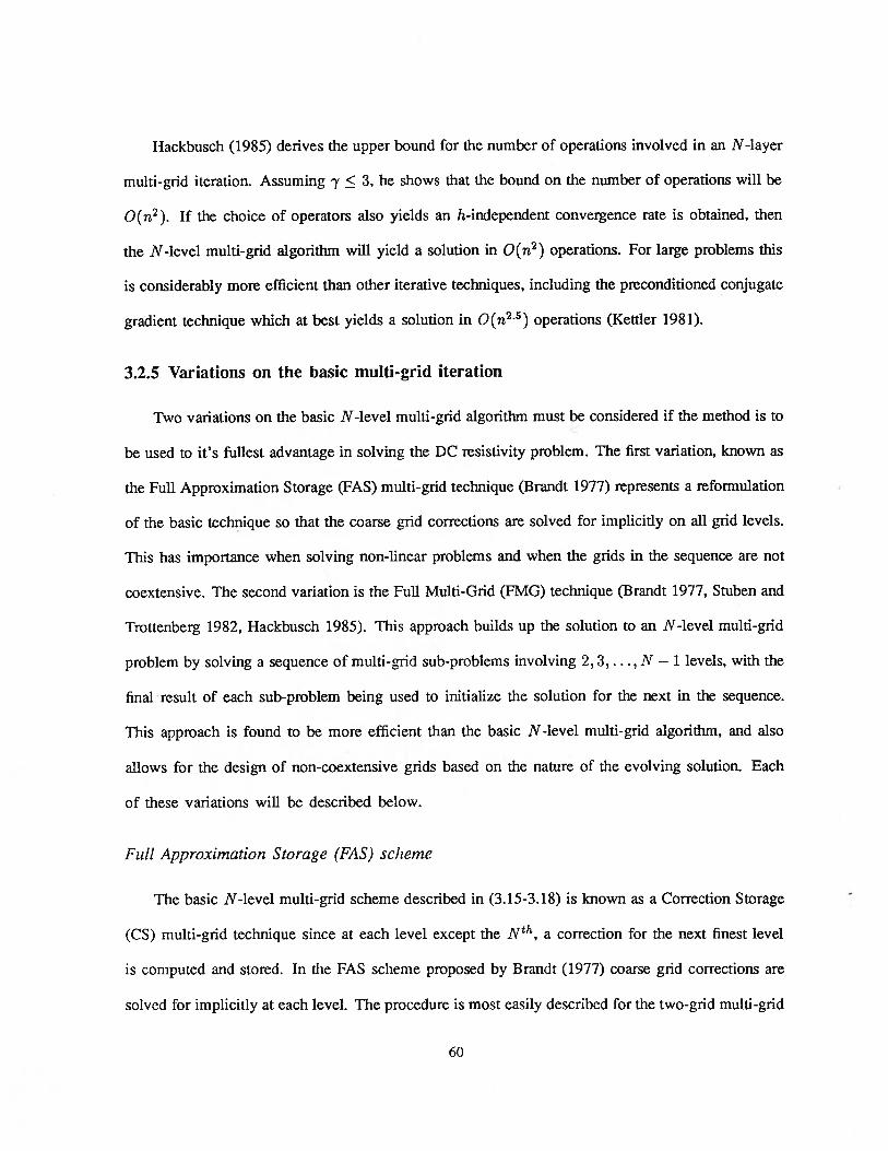
Hackbusch (1985) derives the upper bound for the number of operations involved in an N-layer

multi-grid iteration. Assuming 7 < 3, he shows that the bound on the number of operations will be

0(n2). If the choice of operators also yields an h-independent convergence rate is obtained, then

the N-level multi-grid algorithm will yield a solution in 0(n2) operations. For large problems this

is considerably more efficient than other iterative techniques, including the preconditioned conjugate

gradient technique which at best yields a solution in 0(n25)operations (Kettler 1981).

3.2.5 Variations on the basic multi-grid iteration

Two variations on the basic N-level multi-grid algorithm must be considered if the method is to

be used to it’s fullest advantage in solving the DC resistivity problem. The first variation, known as

the Full Approximation Storage (FAS) multi-grid technique (Brandt 1977) represents a reformulation

of the basic technique so that the coarse grid corrections are solved for implicitly on all grid levels.

This has importance when solving non-linear problems and when the grids in the sequence are not

coextensive. The second variation is the Full Multi-Grid (FMG) technique (Brandt 1977, Stuben and

Trottenberg 1982, Hackbusch 1985). This approach builds up the solution to an N-level multi-grid

problem by solving a sequence of multi-grid sub-problems involving 2, 3 — 1 levels, with the

final result of each sub-problem being used to initialize the solution for the next in the sequence.

This approach is found to be more efficient than the basic N-level multi-grid algorithm, and also

allows for the design of non-coextensive grids based on the nature of the evolving solution. Each

of these variations will be described below.

Full Approximation Storage (FAS) scheme

The basic N-level multi-grid scheme described in (3.15-3.18) is known as a Correction Storage

(CS) multi-grid technique since at each level except the NtI, a correction for the next finest level

is computed and stored. In the FAS scheme proposed by Brandt (1977) coarse grid corrections are

solved for implicitly at each level. The procedure is most easily described for the two-grid multi-grid

60

iteration. Let Üh be an initial approximation to the fine grid solution iZh. As before, v1 iterations of a

relaxation scheme are used to smooth the initial error, and the residual f = — Lhüh is computed

and transferred to the coarse grid. As well, the approximation to the fine grid solution, ith, is also

transferred to the coarse grid. This is denoted by

UH = 11’Uh (3.19)

where ]T1 is another restriction operator, possibly different from the one used to transfer the residual.

After transferring the residuals to 1H. the correction is computed implicitly by solving

LHZH = LHfIH + TH (3.20)

The correction i3’H — UH is then transferred to h, where it is used to correct This is

denoted by

Uh Uh +I(H UH) (3.21)

It is not appropriate to simply transfer H to the fine grid since only corrections can be interpolated

accurately without introducing aliased energy back into the fine grid solution. The sequence of

operations involved in a single two-level FAS iteration is shown in (3.22).

SZ2h

Vh=I.(WH—11H) —f “(322)

I 1’=]f =Ij —+ LHH=LffH+7H

Generalization of the two-level FAS iteration to an N-level FAS iteration is straightforward.

From (3.22) it is clear that the correction computed using FAS will be identical to that computed

using the CS approach. The advantage of using FAS is that the approach can be used even if the

problem is non-linear. As well, if I is chosen to be the injection operator, then the solutions h

and ÜH both converge to uh. This is important if the coarse and fine grids are not coextensive, since

the coarse grid can then be used to solve for corrections to the fine grid solution and a coarse grid

solution simultaneously. This is not possible in the CS formulation where only corrections can be

solved for on the coarse grid.

61

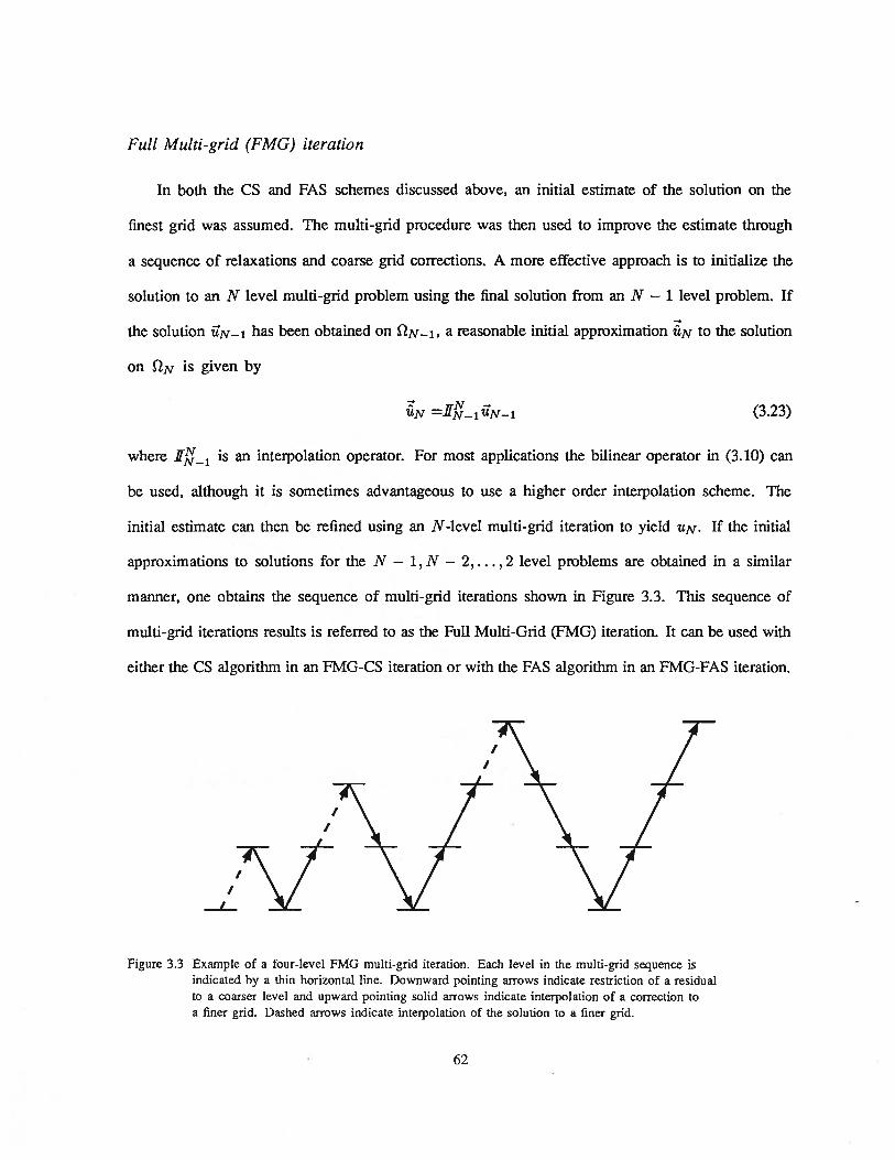
Full Multi-grid (FMG) iteration

In both the CS and FAS schemes discussed above, an initial estimate of the solution on the

finest grid was assumed. The multi-grid procedure was then used to improve the estimate through

a sequence of relaxations and coarse grid corrections. A more effective approach is to initialize the

solution to an N level multi-grid problem using the final solution from an N — 1 level problem. If

the solution tiN—i has been obtained on a reasonable initial approximation UN to the solution

on N is given by

UN ffLiUN_1 (3.23)

where I is an interpolation operator. For most applications the bilinear operator in (3.10) can

be used, although it is sometimes advantageous to use a higher order interpolation scheme. The

initial estimate can then be refined using an N-level multi-grid iteration to yield ‘uN. If the initial

approximations to solutions for the N — 1, N — 2,. . . , 2 level problems are obtained in a similar

manner, one obtains the sequence of multi-grid iterations shown in Figure 3.3. This sequence of

multi-grid iterations results is referred to as the Full Multi-Grid (FMG) iteration. It can be used with

either the CS algorithm in an FMG-CS iteration or with the FAS algorithm in an FMG-FAS iteration.

Figure 3.3 Example of a four-level FMG multi-grid iteration. Each level in the multi-grid sequence isindicated by a thin horizontal line. Downward pointing arrows indicate restriction of a residualto a coarser level and upward pointing solid arrows indicate interpolation of a correction toa finer grid. Dashed arrows indicate interpolation of the solution to a finer grid.

I/

/

/

62

3.2.6 Applications of multi-grid methods to DC resistivity modeling

Because of its small memory requirements and h-independent convergence rate, the multi-grid

technique is well suited to the solution of large-scale pole-pole DC resistivity problems. Since it

is a technique that has never been applied to this geophysical problem, it was unclear how well it

would perform. The goal of this research was to apply the multi-grid algorithm to the modeling

of pole-pole DC resistivity data, and to examine the convergence properties of the algorithm for

different conductivities and source-receiver geometries. To this end, a flexible N-level multi-grid

code was developed to model the transformed potential responses. The development and testing of

the multi-grid algorithm is detailed below.

Several aspects of the pole-pole DC resistivity problem must be considered when developing

an appropriate multi-grid algorithm. Discontinuities and corners in the material properties, source

singularities associated with the current electrode and/or distributed secondary sources, and the use

of non-Dirichiet boundary conditions could potentially degrade the convergence rate of an iterative

solution. The design of the various multi-grid operators must take these aspects of the problem into

account if an acceptable convergence rate is to be maintained. The design of the multi-grid operators

that were used in the solution of the pole-pole DC resistivity problem is detailed below.

Relaxation

For a relaxation scheme to work well in a multi-grid algorithm it must act as an effective smoother

of the error. Since the low frequency components of the error are computed on the coarser grids in

the sequence, the convergence of these components is less ctitial.

To assess the smoothing properties of a particular relaxation scheme, Fourier methods can be

used (e.g. Brandt 1977, Stuben and Trottenberg 1982). Since only changes in local features of the

solution are of interest, details of the domain and the model can be ignored for the analysis. The

63

material properties of the medium can be “frozen” (i.e. assumed equal to some constant) and the

action of the relaxation operator on a Fourier component of the error can be examined.

Although local Fourier analysis is not valid for problems with rapid variations in the material

properties or non-uniform grid spacing, it can still serve as a guide for selecting an appropriate

relaxation scheme. It is well known from local Fourier analysis, for example, that point relaxation

schemes display very poor smoothing rates for strongly anisotropic problems. In these cases there

is a decoupling of the solution in the two directions corresponding to the major and minor axis of

anisotropy. To obtain a good smoothing rate, the solution along lines parallel to the major axis

must be relaxed simultaneously. This suggests the use of a line relaxation scheme as a smoother for

strongly anisotropic problems. For problems with strong discontinuities in the material properties,

a similar decoupling of the solution also occurs between different blocks in the model. The need

to use block or alternating direction line relaxation as a smoother for these type of problems has

been discussed by several authors (e.g. Alcouffe et al 1981, Rude and Zenger 1985). Kettler (1981)

compares the use of various relaxation schemes and shows that line relaxation schemes are superior

to point relaxation when discontinuities are present. Thus, to allow for the possibility of strong

discontinuities in the conductivity, alternating direction Gauss-Seidel line relaxation (e.g. Lapidus

and Pinder 1982) was selected as the smoothing operator for the DC resistivity problem.

Besides the basic line relaxation smoother, several variations were also examined. Because of

the localized nature of the source terms for both the total and secondary potential problems it was

felt that partial relaxations, as suggested by Brandt (1977) and Bai and Brandt (1987), could be used

to improve the overall multi-grid convergence rate. At each iteration this involved using additional

point Gauss-Seidel relaxation sweeps around source locations. This was also used in the vicinity of

corners in the model, where large, high frequency residuals often remained after the basic smoothing

cycle was complete. The use of the partial relaxation strategy was found to yield a somewhat

improved convergence rate. Another variation on the basic smoother was to make use of a simple

64

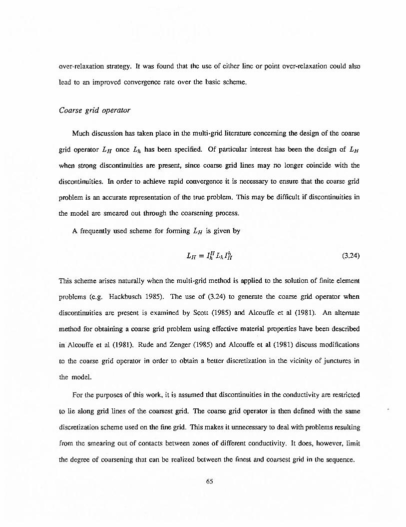
over-relaxation strategy. It was found that the use of either line or point over-relaxation could also

lead to an improved convergence rate over the basic scheme.

Coarse grid operator

Much discussion has taken place in the multi-grid literature concerning the design of the coarse

grid operator LH once Lh has been specified. Of particular interest has been the design of LH

when strong discontinuities are present, since coarse grid lines may no longer coincide with the

discontinuities. In order to achieve rapid convergence it is necessary to ensure that the coarse grid

problem is an accurate representation of the true problem. This may be difficult if discontinuities in

the model are smeared out through the coarsening process.

A frequently used scheme for forming LH is given by

LH = I,’LhI (3.24)

This scheme arises naturally when the multi-grid method is applied to the solution of finite element

problems (e.g. Hackbusch 1985). The use of (3.24) to generate the coarse grid operator when

diseontinuities are present is examined by Scott (1985) and Alcouffe et al (1981). An alternate

method for obtaining a coarse grid problem using effective material properties have been described

in Alcouffe et al (1981). Rude and Zenger (1985) and Alcouffe et al (1981) discuss modifications

to the coarse grid operator in order to obtain a better discretization in the vicinity of junctures in

the model.

For the purposes of this work, it is assumed that discontinuities in the conductivity are restricted

to lie along grid lines of the coarsest grid. The coarse grid operator is then defined with the same

discretization scheme used on the fine grid. This makes it unnecessary to deal with problems resulting

from the smearing out of contacts between zones of different conductivity. It does, however, limit

the degree of coarsening that can be realized between the finest and coarsest grid in the sequence.

65

Solver on coarsest grid

Since the coarsest grid is visited frequently during a single multi-grid iteration, a direct solver

based on the Cholesky decomposition was selected as the solver for the coarsest grid. This takes full

advantage of work done in factorizing the coarse grid coefficient matrix since the same factors can

be used to solve for all coarse grid corrections for each current electrode location.

Restriction of residuals

Because of the presence of discontinuities in the conductivity and singular source terms, the

residuals that are calculated after the first smoothing phase will still contain considerable high

frequency energy (Alcouffe et al 1981). To prevent aliasing, it is necessary to smooth the residuals

before transferring them to the coarse grid. This suggests the use of the full weighting restriction

operator (3.8). Using this operator, a weighted average of the residuals in the vicinity of the

injection point are computed prior to injection. The weighting scheme is illustrated in Figure 3.4.

Since weighted averages of the residuals are transferred, components of the residual that cannot be

represented on the coarser grid are effectively eliminated.

Figure 3.4 Full weighting restriction from fine grid to coarse grid. The coarse grid solution is a

weighted average of the solutions on the fine grid.

c2h

66

Another consideration in deciding on an appropriate restriction operator is the relative weighting

of residuals in different regions of the model. From the form of the truncation error for the DC

resistivity problem it is clear that residuals will be scaled by the conductivity on either side of a

discontinuity. Rude and Zenger (1985) suggest scaling the residuals by the reciprocal of the local

conductivity before using a full weighting restriction. The residuals on the coarse grid can then be

re-scaled by the conductivity. This modified full weighting operator and the usual full weighting

operator were both incorporated into the CS and FAS multi-grid codes. For restriction of the solution

in the FAS code, the injection operator (3.7) was selected. The operator is illustrated in Figure 3.5.

Figure 3.5 Injection from fine grid to coarse grid. For fine grid nodes corresponding to coarse grid nodes

the fine grid solution is simply transferred to the coarse grid.

Interpolation of corrections

Previous work by Alcouffe et al (1981) and Rude and Zenger (1985) describe problems that

can be encountered when simple interpolation schemes are used for the coarse to fine correction

transfers across a discontinuity. Since it has been assumed in this case that all discontinuities in the

conductivity lie along grid lines of the coarsest grid, this problem cannot arise. Thus the bilinear

interpolation operator given in (3.10) was used to interpolate corrections in both the FAS and CS

codes. The interpolation scheme is illustrated in Figure 3.6.

67

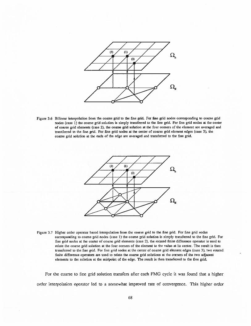
Figure 3.6 Bilinear interpolation from the coarse grid to the fine grid. For fine grid nodes corresponding to coarse grid

nodes (case 1) the coarse grid solution is simply transferred to the fine grid. For fine grid nodes at the center

of coarse grid elements (case 2), the coarse grid solution at the four corners of the element are averaged andtransferred to the fine grid. For fine grid nodes at the center of coarse grid element edges (case 3), thecoarse grid solution at the ends of the edge are averaged and transferred to the fine grid.

Figure 3.7 Higher order operator based interpolation from the coarse grid to the fine grid. For fine grid nodescorresponding to coarse grid nodes (case 1) the coarse grid solution is simply transferred to the fine grid. Forfine grid nodes at the center of coarse grid elements (case 2), the rotated finite difference operator is used torelate the coarse grid solution at the four corners of the element to the value at its center. The result is thentransferred to the fine grid. For fine grid nodes at the center of coarse grid element edges (case 3), two rotatedfinite difference operators are used to relate the coarse grid solutions at the corners of the two adjacentelements to the solution at the midpoint of the edge. The result is then transferred to the fine grid.

For the coarse to fine grid solution transfers after each FMG cycle it was found that a higher

order interpolation operator led to a somewhat improved rate of convergence. This higher order

68

interpolation operator was obtained using a rotated finite difference scheme (Figure 3.7). Although

a scheme using cubic interpolation was considered, it would have required the use of less accurate

one-sided operators in the vicinity of discontinuities, and was not implemented.

3.2.7 Examples — convergence rates for various models and operators

To illustrate the convergence properties of the multi-grid algorithm, the problem illustrated in

Figure 3.8 was considered. The model consists of a pair of 1000 m prisms buried in a 10 m

halfspace. Note that the prisms meet at a juncture located at (x, z) = (250, 100) m. A current

electrode at (x, z) = (0, 0)m is used to inject a current of iDA.

l000Qm I150 m

_L.. 1000 2m

10 2m

I 250m I

Figure 3.8 Two prism problem used to illustrate the convergence properties of the multi-grid forward modelingalgorithm. The model consists of a pair of 1000 m resistive prisms in a 10 flm halfspace.

An initial discretization of the two-prism problem is superimposed over the model in Figure 3.9.

This was used as the coarse grid in an FAS-FMG solution of the transformed secondary problem

for k = 0.001 rn1. Parameters -y = 2, i-’ = 2, v2 = 1 were selected for the multi-grid iterations

in this example.

69

500.0

—1000.0 0.0 1000.0

Distance (m)

Figure 3.9 Coarsest grid in the multi-grid discretization of the problem in Figure 3.8. A verticalexaggeration of 4 times was used in the display.

To determine the convergence rate of the multi-grid algorithm, the errors in the fine grid solution

and the residuals were monitored for a sequence of two-level multi-grid iterations. The maximum

absolute error and the maximum absolute residual are plotted as functions of operation number in

Figures 3. lOa and 3. lOb respectively. Operations include the interpolation of the coarse grid solution

to the fine grid (square), fine grid relaxations (triangles) and coarse grid corrections (stars). Each

multi-grid iteration is seen to reduce the maximum absolute error by a factor of 10 or more. A similar

reduction in residual is also observed. In particular, rapid decreases in the error occur after each coarse

grid correction, demonstrating the role of the coarse grid correction in accelerating convergence of

the relaxations. Note that in some cases the coarse grid correction actually leads to an increase in

the maximum absolute residual — a rapid decrease being observed only after the second smoothing

phase. The coarse-to-fine grid interpolation has clearly generated additional high frequency residuals.

Hence the need for the second smoothing phase prior to transfer of the solution to the next leveL

0.0

4J

G)

70

100 — 10—1

101 10—2

E

? 10-2 s—

0

2io—3 io

EE

E iO 10

iO 10-s

10—6 II

io—

0 5 10 15 0 5 10 15Operation number Operation number

Figure 3.10 Convergence of the two-level multi-grid solution for the problem in Figure 3.8. (a) The maximumabsolute error in the fine grid solution for each multi-grid operation. (b) The maximum absoluteresidual for each operation. The interpolation of the coarse grid solution is indicated by asquare, relaxations by triangles and coarse grid corrections by stars.

Profiles of the transfomed secondary potentials computed using two, three and four-level multi-

grid iterations are shown in Figure 3.1 la. Note that there are large changes in the solution as

more grids are added to the sequence. This indicates an underlying problem in the finite difference

discretization in the vicinity of the corners and, in particular, at the juncture where the two prisms

meet. This aspect of the problem will be discussed in detail in Chapter 4. The maximum absolute

residual for each solution is shown as a function of iteration number in Figure 3.1 lb. Although the

goal of h-independence has not been fully realized, the overall convergence rate for the multi-grid

algorithm is seen to be excellent. Only a single iteration on the finest grid is needed, for example,

to reduce the maximum absolute residual by a factor of about 50.

a. b.

20 20

71

1.8— 10-1

10-21.6

1.4 ‘? io-- io-

E 1.2

i.o ia-7.2 ‘ -8— ‘- IVC V.0

F i090.6

0.4

0.210—13

0.0 10-14I I

—1000 1000 0 2 4 6Iterotion number

Figure 3.11 Results of a two, three and four-level multi-grid solution for the problem in Figure

3.8. (a) Profiles of the final transformed potentials on each of the four levels. (b) Themaximum absolute residual for each multi-grid iteration.

Since the convergence rate of the multi-grid algorithm depends on the choice of operators used,

it is worth examining different variations to see if improvements in efficiency can be achieved.

Convergence rates for the four-level multi-grid scheme using different coarse grid correction operators

are compared in Figure 3.12 to the convergence rate achieved using the basic scheme (shown dashed).

In Figure 3. 12a, V-cycle iterations were used instead of W-cycles, resulting in a poorer convergence

rate. Although more expensive, the W-cycle iteration was found to be more efficient in terms of

execution time needed to achieve a given reduction in the maximum absolute error. In Figure 3. l2b,

the higher order interpolation scheme described earlier was used instead of bilinear interpolation,

without a significant improvement in accuracy. In Figure 3.12c, injection was used as the restriction

operator for the residuals, resulting in a dramatic deterioration in the convergence rate. The transfer

of residuals in the DC resistivity problem clearly results in significant aliasing unless the residuals are

filtered prior to injection. In Figure 3. l2d, the conductivity scaled full-weighting scheme proposed by

Rude and Zenger (1985) led to no significant improvement over the standard full-weighting scheme.

a. b.

0X position (m)

8 10

72

10—1 10-1

102 102

io— —S iD

iD—i - iD-i

- ic-s iO-D

io-

io-E F

io— i0

ic—9 iO

10_la 10—10

b_fl bO_fi

10—12 10—120 2 4 6 8 10

Iteration number

10—1 10-1

10-2 10-2

iO— —S

io— . io-

3 i0 i0D

io- .2 1065) 5)L i— ‘- io-

io io

io‘ 10-g

io—° i0

10_il 10

10—12 I I 10—12 II

0 2 4 6 8 10 0 2 4 6 8 10

Iteration number Iteration number

Figure 3.12 Convergence rates of the four-level multi-grid algorithm for the problem in Figure 3.8. Resultsobtained using different multi-grid operators (solid lines) are compared to that obtained usingthe basic algorithm (dashed). (a) V-cycle iterations used instead of W-cycle iterations. (b) Higher

order inteqolation of solution used in FMG iteration. Cc) Injection instead of full-weighting restriction.(d) Conductivity scaled full-weighting used instead of full-weighting restriction.

In addition to studying different transfer operators and cycling strategies, various relaxation

schemes were also examined to detemfine the optimum procedure. Point Gauss-Seidel relaxation

iterations were used instead of line relaxations to yield the results in Figure 3.1 3a. The convergence

rate for the multi-grid iteration using point relaxation is clearly inferior to that using the line

relaxation scheme. If 8 point relaxation sweeps were perfonned for every line relaxation sweep,

then the convergence rate approaches that of the basic multi-grid scheme (Figure 3.13b). The cost

a. b.

0 2 4 6 8 10

Iteration number

d.\

73

of performing such a large number of point relaxations, however, makes this a less efficient strategy.

The use of over-relaxation, with a relaxation parameter of 0.5, leads to a marked improvement in

the convergence rate of the single point Gauss-Seidel iteration (Figure 3. 13c). Results with other

models and wavenumbers, however, indicate that the optimum relaxation parameter is very problem

dependent and may in practice be difficult to determine a priori. The use of partial relaxation in the

10—1

10—2

io—io—

E io—io—

‘- io—E

10

•g ic-910-10

10

10_12

10—1

10-2

—‘ iO-

io--ö iO-

10-6

io—io-io-

10_11

10—12

10—1

10-2

__

ic-3i0-

.ö io-io—

E io—g io-

10_li

10_12

10-1

10-2

ic-k- io-

io-ic-v

E10

io-10-10

10_Il

1012

Figure 3.13 Convergence rates of the four-level multi-grid algorithm for the problem in Figure 3.8. Results obtainedusing different relaxation schemes (solid lines) are compared to that obtained using the basic algorithm(dashed). (a) One point Gauss-Seidel relaxation used instead of each line relaxation. (b) Eight pointrelaxations used instead of each line relaxation. (c) One point Gauss-Seidel over-relaxation used instead ofeach line relaxation. A value of 0.5 was used for the over-relaxation parameter. (d) Basic line relaxationscheme supplemented with partial relaxations in the vicinity of the juncture in the model.

0 2 4 6 8 10

tercton number

0 2 4 6

Iteration number

C.

a 10

I I

0 2 4 6 8 10 0 2 4 6

Iteration number Iteration number

8 10

74

the vicinity of the juncture leads to an improved convergence rate (Figure 3.1 3d) without adding

significantly to the cost of the solution.

The perfonnance of the multi-grid algorithm was also studied for a wide variety of models and

source configurations. The convergence rates observed were very similar to those described above.

One factor that was found to influence the convergence rate of the algorithm was the wavenumber

being modeled. The multi-grid algorithm was found to converge more quickly for larger wavenumbers

(Figure 3. 14a). The nature of the model was also found to influence the convergence rate. In Figure

3. 14b, results for a more resistive and less resistive set of prisms were compared to those from the

previous model. The lower resistivity contrast yielded much better convergence rates, while the

higher resistivity prisms resulted in a somewhat poorer rate. In general it was found that resistive

targets, as in the example, yielded the slowest convergence. The proximity of the current electrode

to resistive corners in the model seemed to be the primary cause of the poorer convergence rate.

b.10-1 10-1

10—2 10-2

iO- —.- ic-3

1O . ic-i_5 1O— 5 iO-

io- . i0-C

i07 ‘- ic-7E E ic-s

-g io- g10—10 10—10

10—11 10—11

10—12 10—120 2 4 6 8 10

Iteration number

Figure 3.14 Convergence rates of the four-level multi-grid algorithm for variations on the problem in Figure 3.8. Results

obtained using different wavenumbers and conductivity contrasts (solid lines) are compared to that

obtained for the problem in Figure 3.8. (a) Results for wavenumbers of 0.01 rn_i and 0.0001 m1

(solid lines) are compared to those for 0.001 rn1 (dashed). (b) Results for prism resistivities of

100 fm and 10, 000 2m (solid lines) are compared to those for 1000 2m (dashed).

0 2 4 6 8 10Iteration number

I I I

75

It was found that the convergence rates depicted in Figures 3.12-3.14 were typical, and that the

algorithm was well suited to the solution of the DC resistivity problem. The multi-grid algorithm was

used to model transformed potentials for a range of wavenumbers, and the solution on each level was

inverse Fourier transformed. The results are shown in Figure 3.15a. The solution is seen to change

considerably between each grid level, indicating a problem with the underlying discretization. This

problem will be discussed in Chapter 4, and a method of extrapolating the solution will be presented.

The same model was used to study the solution of total potentials using the multi-grid algorithm.

Similar convergence rates were observed as with the modeling of secondary potentials. The apparent

resistivities computed for the total potential problem using the four-level multi-grid solution is shown

in Figure 3. 15b. As before, the solution changes considerably between each grid level.

b.18 —

0.00017

0.0025

-

16

c’ 0.0020 /> 15

0015 1 :V

12

0.0005 11

0.00009 _1____ -

—1000 0 1000 —1000 1000X pstion (m) X poston (m)

Figure 3.15 Four-level multi-grid solution for the problem in Figure 3.8. (a) Profiles of the secondary

potentials on each of the four levels. (b) Profiles of the apparent resistivites computed

from the total potentials on each of the four levels.

A comparison of the multi-grid results (triangles) on the fourth level to those obtained using

a direct solver (solid line) was used to verifly the multi-grid procedure (Figure 3.16). Only two

iterations for the smaller wavenumbers, and a single iteration for the larger wavenumbers were

needed to achieve a fit of less than 0.5% over the entire profile. The execution time required to solve

0

76

the fine grid problem directly was 1059.2 cpu seconds on a Sun 4/330. The time required to obtain

each multi-grid solution was 41.6 cpu seconds.

I0

0.003017

0.0025

‘0.0020 >15

140.0015

C

0 —

° 0.0010 12

0.0005 -11

100.0000

I 9’—1000 1000 —1000 0 1000

X position (m) X position (m)

Figure 3.16 Comparison of the solutions computed using a direct solver (solid line) and the four-level multi-gridsolver (triangles> for the problem in Figure 3.8. (a) Profile of the secondary potentials computed on thefinest level. (b) Profile of the apparent resistivities computed on the finest level.

3.3 The multi-level adaptive technique

A variation of the multi-grid procedure, originally proposed by Brandt (1977), is the Multi-Level

Adaptive Technique (MLAT). In this strategy, a sequence of non-coextensive grids is constructed as

the solution is being calculated — the spatial extent of the grids in the sequence being based on the

nature of the evolving solution. This allows both the grid design and solution processes to be carried

out simultaneously, resulting in considerable computational savings. Although the algorithmic details

of the MLAT strategy have been described in the literature, it’s application to practical problems has

been somewhat limited. This is primarily due to the general complexity of the algorithm and the need

for a suitable grid refinement criterion. The purpose of this research was to apply the multi-level

algorithm to the solution of the pole-pole resistivity problem. A new criterion for grid refinement

based on an analysis of the relative truncation error will be described in Chapter 4.

a. b.

0

I

77

3.3.1 Multi-level adaptive technique

Consider first the solution of the general problem (3.1) using the standard multi-grid approach.

The sequence of grids f2,.. ., 1Zi,... is used to obtain a solution on the finest grid where

the coarser grids in the sequence are used to accelerate convergence of the relaxation scheme on

N by providing a low frequency correction to the fine grid solution. One of the basic assumptions

in the standard multi-grid algorithm is that the N grids in the sequence completely overlap, or are

coextensive (Figure 3.17). In most cases, however, the use of coextensive grids is very inefficient.

With the DC resistivity problem, for example, only portions of the domain adjacent to sources and

discontinuities in the conductivity require a fine discretization. The remainder of the domain can be

discretized quite coarsely without affecting accuracy. Although a non-uniform grid spacing can be

used at each grid level to achieve different degrees of resolution in different parts of the domain,

this is still not optimal. The use of non-uniform grid spacing with the finite difference technique

invariably leads to a large number of long, thin elements towards the edge of the grid. As well, a

non-uniform discretization is considerably less accurate than a uniform one.

Figure 3.17 A sequence of three coextensive grids used in the standard multi-grid iteration. Each gridcompletely overlaps the previous grids in the sequence.

78

A more efficient approach is to make use of a sequence of non-coextensive grids, as shown in

Figure 3.18. By allowing the size of each successive grid in the sequence to become smaller, the

extent of the fine grids can be restricted to only those regions where a fine discretization is needed to

achieve the desired accuracy. The coarser, more extensive grids are used only to satisfy the boundary

conditions and to accelerate convergence of the solution on the finer grids. Using this strategy, the

fine grids can be made considerably less extensive than in a standard multi-grid solution. Thus the

total computational work expended in obtaining a solution can be dramatically reduced.

Figure 3.18 A sequence of three non-coextensive grids. The finer grids extend over only a

sub-region of the coarser grids in the sequence.

If all grids in the multi-grid sequence are coextensive, then the solution can be obtained using

either the CS or FAS schemes. If the grids are not co-extensive, then the CS scheme cannot be used.

Recall that in the CS scheme the problem that must be solved on the kth grid, Qk, is given by

Lkk = = — rk+1) (3.25)

This yields the correction ‘15k that is then interpolated to and used to correct k+1• If 12,-- does

not completely overlap k, then the CS formulation breaks down since one cannot simultaneously

c1

79

solve for both ‘7k outside the region of overlap and k within the region of overlap. For this reason

the FAS scheme must be used for problems involving non-coextensive grids.

Let k be the portion of k that k+1 overlaps. An FAS scheme suitable for use with non-

coextensive grids can be obtained by considering the problem

LkUk = fk (3.26)

whereUk=Ikk+lUk+1+Vk °

(3.27)

Uk Ofl kk

and7 rrrk — rk f r —

Jk = .L,kL1k+lUk+1 + ‘k+l ik+1 — .LIk+lUk+1) Ofl Lk

(3.28)

fk Ofl 12kk

Since the boundaries of k+1 may not correspond to those of k, new boundary conditions must be

specified before Lk+l can be formed. One way of doing this is to apply Dirichlet boundary conditions

along Dlk+1, where the values of Uk+1 at boundary nodes are obtained by interpolating Tip, from 2j.

To examine how the fine and coarse grids interact in this scheme, note that for a two-level

iteration, the coarse grid problem can be written as

- -H H= fH + Th + ‘h 7h (3.29)

where only the portion of the grid in the region of overlap is considered. The quantity =

LHKjüh — is clearly an estimate of the relative truncation error 4 based on the approximate

solution to the fine grid problem. At convergence, h = 0, so that the coarse grid problem will be

corrected by the addition of to its right hand side in the region of overlap. In this way, fine grid

accuracy is transmitted to the coarse grid even if the grids do not fuliy overlap.

The MLAT algorithm proposed by Brandt (1977) makes use of the FAS scheme described

above to adaptively design a sequence of non-coextensive grids around the solution as it is being

calculated. Assume that a solution has been obtained using the sequence of non-coextensive grids

80

Sl2,. . . ,!2r_. Based on some grid refinement criterion, a subregion of N—1, denoted by c2N.1,

is identified as being too coarse. This subregion of 2N—1 is refined, yielding the next grid in the

sequence, 11N The solution on N—1 is then interpolated to and it becomes the initial estimate

for the fine grid solution. The non-coextensive FAS algorithm is then used to correct this initial

estimate, yielding UN. The algorithm is terminated when the change in the solution due to the

addition of the next finest grid is less than some tolerance.

Figure 3.19 A sequence of composite grids where hanging nodes (indicated by dots) have been tied

in to the rest of the grid using rotated finite difference operators.

In the development of an MLAT solution to the pole-pole DC resistivity problem, an approach

similar to that of McCormick and Thomas (1986) was adopted. To form a fine grid in this scheme,

rotated finite difference operators are used to relate fine grid boundary nodes to coarse grid nodes

(Figure 3.19). Relaxations are carried out only over the square portion of the fine sub-grids. In

calculating the residuals for transfer to the next coarser grid, Dirichlet boundary conditions are not

assumed along the boundaries of the sub-grid, as they are in the original MLAT formulation. Instead,

the rotated operator is used to compute the residual as if the entire composite grid had been relaxed.

81

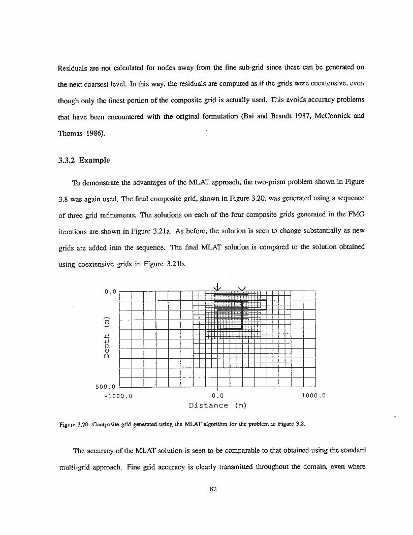
Residuals are not calculated for nodes away from the fine sub-grid since these can be generated on

the next coarsest level. In this way, the residuals are computed as if the grids were coextensive, even

though only the finest portion of the composite grid is actually used. This avoids accuracy problems

that have been encountered with the original formulation (Bai and Brandt 1987, McCormick and

Thomas 1986).

3.3.2 Example

To demonstrate the advantages of the MLAT approach, the two-prism problem shown in Figure

3.8 was again used. The final composite grid, shown in Figure 3.20, was generated using a sequence

of three grid refinements. The solutions on each of the four composite grids generated in the FMG

iterations are shown in Figure 3.21a. As before, the solution is seen to change substantially as new

grids are added into the sequence. The final MLAT solution is compared to the solution obtained

using coextensive grids in Figure 3.21b.

w

::L: L!t!J4J

a)

500.0

—1000.0 0.0 1000.0

Distance (m)

Figure 3.20 Composite grid generated using the MLAT algorithm for the problem in Figure 3.8.

The accuracy of the MLAT solution is seen to be comparable to that obtained using the standard

multi-grid approach. Fine grid accuracy is clearly transmitted throughout the domain, even where

82

the fine grid is not present. Because of the limited extent of the finest grids, however, the MLAT

algorithm is considerably more efficient than the standard multi-grid algorithm. In this case, the cpu

time required for the four-level multi-grid solution using coextensive grids was about 6 times that

required to generate the MLAT solution. A further extension of this approach that would allow for

the evolution of more than one fine grid sequence would result in even better efficiency.

1.8 1.8’

1.6 1.6

1.4 1.4

1.2> >— 1.0 ‘ 1.0.20.8

5)

0.6

0.4 0.4

0.2 0.2

0.0 0.0’

—1000 1000 —1000 1000

Figure 3.21 Transformed secondary potentials computed using the MLAT algorithm for the problem in Figure 3.8. (a)

The transformed secondary potentials computed at each stage of the FMG sequence. (b) The final MLAT

solution (triangles) compared to the multi-grid solution obtained using coextensive grids (solid line).

3.4 Conclusions

The use of the multi-grid approach to the solution of the DC resistivity forward problem was

found to yield accurate results for both total and secondary potential problems. The convergence rate

for a proper choice of multi-grid operators was found to be excellent. Because of the small memory

requirements of the algorithm much larger problems could be solved than would be possible with the

direct Cholesky solver. The speed of the algorithm, even when a large number of current electrodes

was being modeled, was considerably better than could be achieved with the direct solver.

In addition to the efficiency of the algorithm, the full multi-grid algorithm also yielded solutions

on a sequence of grids of increasing fineness, allowing the accuracy of the solution on the finest

0. b.

0X poSition (m)

0X position (m)

83

grid to be assessed. For many problems that have been examined the solution was found to change

lithe between grid levels once a reasonable degree of refinement had been achieved. In other cases,

including the problem illustrated here, large changes were observed even between relatively fine

grids, indicating an underlying problem with the discretization and the need for further refinement.

The development of a multi-level approach, where finer grids in the sequence were permitted

to become spatially less extensive, also led to an efficient forward modeling algorithm. The use of

non-coextensive grids permitted the region around singularities and rapid changes in the material

properties to be detailed, without the need for refining the entire grid. A strategy that was found

useftil was to design a 2 or 3 level sequence of coextensive grids around the model, and to use an

additional 2 or 3 levels of non-coextensive grids to refine the area around the current electrode. The

refinement grids are then moved with the current electrode, while the coextensive grids remain fixed.

This provided a systematic approach to the grid refinement process, and allowed for an accurate

discretization for all current electrode positions. The additional flexibility of allowing for multiple

refinement sequences would have made the multi-level solver even more efficient.

84

Chapter 4

Adaptive Grid-design Using the Multi-grid Approach

4.1 Introduction

Because of the difficulty of estimating the accuracy of a numerical solution a priori, it is important

that a direct verification of accuracy be made before the solution can be considered reliable. The usual

approach for verifying the overall accuracy of a numerical algorithm is to compare the numerical

results to analytic solutions for simple model geometries. Although this is useful for debugging

purposes, it is impossible to assess the accuracy of an algorithm for more general models based on

this kind of comparison. A way of verifying the accuracy of a numerical solution for a specific model

and electrode configuration is needed. A simple way of doing this is by re-solving the numerical

problem using a more accurate discretization, and observing how much the solution changes. This

approach can be extremely expensive, however, if standard methods are used.

If the numerical solution for a particular model is found to be inaccurate, steps must then be

taken to improve the discretization. Because there is a trade-off between accuracy and computational

expense, this improvement cannot be based solely on the desire to compute a highly accurate solution.

A procedure is needed for designing a discretization that achieves a specified error level while

minimizing the computational work required. The desigu of such an “optimum” discretization

is particularly desirable in two and three dimensional problems where the number of operations

involved in a forward solution can become quite large. Although a truly optimum discretization

85

is never attainable, a near-optimum solution can be found through partial refinements of an initial

discretization. Because the numerical error is problem dependent, an “adaptive” approach to the

design of discretization is needed. Ultimately, an algorithm is desired that monitors the accuracy

of a numerical solution and, if necessary, adapts the discretization to the solution itself, providing

a fine discretization only where required.

4.2 Numerical error and grid design considerations

In order to assess the accuracy of a given discretization, and to help in the design of an accurate

numerical grid, one needs to consider the factors that control the error distribution in the solution.

Let u be the solution to the problem

£u=f (4.1)

and let

LiZ=f (4.2)

be the discrete approximation to (4.1). If we let ‘L7cont be the solution to the continuous problem

sampled at each grid point, then 1cont satisfies the problem

LfZ0 = (4.3)

where is the truncation error. Subtracting (4.2) from (4.3) yields the new problem

L= (4.4)

where = —

ii is the error in the numerical solution. The truncation error, f, acts as the source

of numerical error in exactly the same way that the current electrode acts as the source in the original

problem. The magnitude of the error at a particular node in the grid will depend on the strength

of these sources as well as their proximity. Since the sources can be either positive or negative, a

86

certain amount of error cancellation will always occur. In some cases, particularly when the model

displays a high degree of symmetry, this cancellation can result in an error that is small even though

the discretization is quite poor. This has serious implications as far as the testing of numerical codes

with simple analytic solutions is concerned.

4.2.1 Factors controlling truncation error strengths

As can be seen from (2.20), the strength of the truncation error sources will depend not only on

the local grid spacing, but also on local features of the model and the solution. Factors that control

the truncation error in the DC resistivity problem are described below.

Large gradients in the potential

These are particularly important in the DC resistivity problem where localized source distributions

and discontinuities in the conductivity lead to rapid changes in the potential and its derivatives. When

solving for total potentials, the large gradients associated with the logarithmic singularity at the current

electrode lead to large truncation errors at the current electrode node and at the three adjacent nodes

(four adjacent nodes in the case of a buried current electrode). These truncation errors are found to

nearly cancel however, so that the finite difference approximation in the vicinity of the electrode is

still found to be 0(h2) (Bai and Brandt 1987). The resulting error in the numerical solution for a

uniform grid is also found to be 0(h2) (Bai and Brandt 1987, Rude 1988).

When secondary potentials are computed, the point Current electrode is replaced by surface

sources distributed along discontinuities in the model. Although the solution remains finite, rapid

changes in the solution near the discontinuities still lead to large truncation errors.

Another major contribution to the error arises from a singularity that occurs at corners in the

model (Alcouffe et al 1981, Rude and Zenger 1985, Liggett and Liu 1983). At these singular points

the gradients in the potential do not approach a limiting value, so that the expression for the truncation

87

error (2.20) is no longer valid. Rude and Zenger (1985) show that the solution error in the vicinity of

a corner is O(hj where a depends on the angle of the corner and the conductivity contrast. In some

cases a can be quite small, resulting in a large error in the numerical solution which only gradually

decreases as the grid is refined. This slow convergence to the true solution is particularly severe for

highly resistive, small angled wedges and four-corner junctures. Although corner singularities will

be present in both total and secondary potential problems, they are most prominent in the secondary

problem, where sources are placed directly on the corners.

Grid spacing

The truncation error also depends on the local coarseness of the grid, as well as its uniformity. For

a constant conductivity model and uniform grid spacing the 0(h3) terms cancel in (2.20), leaving

only terms of order 4 and higher. For non-uniform grids, if the grid spacing changes quickly so

that one of the 0(h3) terms in (2.20) dominates, a large truncation error may result. Care must

therefore be taken when partially refining an existing grid since the resulting non-uniformity can lead

to significant errors in the solution.

Approximate boundaiy conditions

Since the boundary condition (2.21) used in the numerical problem is only approximate, an error

in the discretization along the right, left and lower boundaries will occur. The resulting distribution of

truncation error will act as a source of error that will decay away from the boundaries, contaminating

the solution towards the center of the grid. By placing the boundaries farther from the source region,

the strength of these truncation errors can be reduced.

Since the truncation error distribution depends on both the model and the current electrode

location, the design of a numerical grid to minimize the resulting error in the solution is problem

88

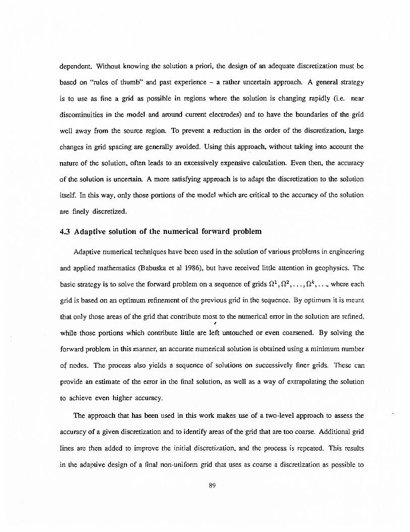
dependent. Without knowing the solution a priori, the design of an adequate discretization must be

based on “rules of thumb” and past experience — a rather uncertain approach. A general strategy

is to use as fine a grid as possible in regions where the solution is changing rapidly (i.e. near

discontinuities in the model and around current electrodes) and to have the boundaries of the grid

well away from the source region. To prevent a reduction in the order of the discretization, large

changes in grid spacing are generally avoided. Using this approach, without taking into account the

nature of the solution, often leads to an excessively expensive calculation. Even then, the accuracy

of the solution is uncertain. A more satisfying approach is to adapt the discretization to the solution

itself. In this way, only those portions of the model which are critical to the accuracy of the solution

are finely discretized.

4.3 Adaptive solution of the numerical forward problem

Adaptive numerical techniques have been used in the solution of various problems in engineering

and applied mathematics (Babuska et al 1986), but have received little attention in geophysics. The

basic strategy is to solve the forward problem on a sequence of grids c, , where each

grid is based on an optimum refinement of the previous grid in the sequence. By optimum it is meant

that only those areas of the grid that contribute most to the numerical error in the solution are refined,4.

while those portions which contribute little are left untouched or even coarsened. By solving the

forward problem in this manner, an accurate numerical solution is obtained using a minimum number

of nodes. The process also yields a sequence of solutions on successively finer grids. These can

provide an estimate of the error in the final solution, as well as a way of extrapolating the solution

to achieve even higher accuracy.

The approach that has been used in this work makes use of a two-level approach to assess the

accuracy of a given discretization and to identify areas of the grid that are too coarse. Additional grid

lines arc then added to improve the initial discretization, and the process is repeated. This results

in the adaptive design of a final non-uniform grid that uses as coarse a discretization as possible to

89

achieve the desired accuracy. The development of this algorithm, and its application to the pole-pole

DC resistivity problem, is described below.

4.3.1 Two-level multi-grid approach to adaptive grid design

As a standard procedure when computing any numerical solution, the forward problem will often

be solved on a pair of grids, the first being one’s best attempt at an accurate discretization based on

experience and rules of thumb. The second grid, being somewhat finer than the original, is used to

assess the accuracy of the numerical solution. If the solution does not change significantly between

the two grids, the numerical solution is then considered to be accurate. If the solution does change

significantly, then the grid must be redesigned to improve its accuracy. The use of an adaptive

approach to grid design based on the two-level multi-grid algorithm is an attempt to formalize this

procedure.

Consider the numerical solution of the general problem (4.1) on a pair of grids f2 and c.

It will be assumed that S2 is obtained through a complete refinement of Note that the grid

spacings can be non-unifonn, even though the constants h and H are used to designate the two grids.

Let the fine and coarse grid solutions iZh and ilH satisfy the discrete problems

= on (4.5)

and

= fi-i on (4.6)

respectively. The relative error, e, which is the error in the coarse grid solution relative to the fine

grid solution, is given by

IjUh — UH (4.7)

Examination of the relative error at selected nodes provides a simple way of verifying the accuracy

of the fine grid solution. A small relative error indicates that the fine grid and coarse grid solutions

have converged and that little improvement will be realized through further refinement.

90

Although the relative error quantifies the improvement in the solution resulting from the refine

ment of the grid, it provides no direct information about which areas of the grid were primarily

responsible for the improvement. To identify areas that contribute most to the relative error, and

hence determine where further refinement is needed, we introduce the relative truncation error,

defined by

=LHI,ith—fH (4.8)

Combining (4.6-4.8) yields

(4.9)

Note that the relative truncation errors at each node act as sources of relative error. To find the

contribution from each of these sources to the relative error at the lj node (called the control node),

the discrete adjoint Green’s function problem

= 8H,l (4.10)

is solved, where 8H1 is zero except for the 1th ent which is one, and is the discrete adjoint

Green’s function. L7 is the adjoint operator corresponding to LH, and is defined such that

— = 0 (4.11)

for all H and ?iH• Since many problems in geophysics are seif-adjoint, L is often found to

be identical to LH. Note that self-adjointness of the continuous problem does not guarantee self

adjointness of the discrete problem unless the discretization is symmetric. In this case, the use of the

integral finite difference scheme leads to a discrete problem which is self-adjoint.

Multiplying (4.10) by (4[)T and (4.9) by (ff11,1)T, and then subtracting yields

—H T -T - -H T -.T II(Ch ) LH — gfJ1LJfc/ = (Ch ) “,i

— 2111’h (4.12)

91

Since (4.11) must be satisijed, the left side of (4.12) is identically zero, and hence

(e’)1 = (.H,1)T?L1 (4.13)

where the summation is taken over all nodes of c. A map of (H,1)j(,,H)j thus yields the

contribution from each part of 1 to the relative error at the control node.

In general, the accuracy of the solution at a number of control nodes (perhaps corresponding to

several field data acquisition locations) will need to be monitored. Since an adjoint Green’s function

problem must be solved for each control node, the use of (4.13) may no longer be practical. A

way of reducing the number of forward problems that must be solved is to define the new discrete

adjoint problem

LH = W([)1H,l (4.14)

where the summation is taken over all nodes in The w1’s are weighting coefficients which are

set to zero except at the control nodes. Using this new adj Dint problem, one obtains

= = (4.15)

Thus a map of (ff)(q) yields the contribution from each part of the coarse grid to the relative

error energy ER = w?(4’). The use of (4.15) to compute the error contribution map is very

efficient since only a single adjoint Green’s function must be computed in this case.

Being able to identify regions of the grid that contribute the most to the relative error or relative

error energy allows a grid refinement procedure to be formulated. Assume first that a grid f

is available from the previous grid refinement. A fine grid ! is generated through a complete

refinement of !. This involves adding an additional grid line midway between each of the original

grid lines. A direct solver employing a Cholesky factorization is then used to compute ijj on

An initial approximation to the fine grid solution, üj1 can be obtained by interpolating ‘H to

92

Bccausc the same forward problem must be solved on both a coarse and fine grid, it would

be desirable if work done in calculating the coarse grid solution could be used to reduce the work

required on the fine grid. This suggests the use of the two-level multi-grid algorithm to improve

the initial approximation to the fine grid solution. Since a Cholesky decomposition is used to solve

the coarse grid problem for iZH, the factors can be used again to solve for each of the coarse grid

corrections, making this a very efficient iteration.

Once a satisfactory fine grid solution has been obtained, it is transferred to the coarse grid

and used to compute the relative truncation error using (4.8). The Green’s function is computed

by solving either (4.10) or (4.14). Again, the factors of the coefficient matrix generated from the

solution of the coarse grid problem can be used to compute the Green’s function on Finally,

the appropriate error contribution map is generated using either (4.13) or (4.15).

In most cases, only isolated regions of % will contribute significantly to the relative error or

relative error energy. This suggests carrying out a partial refinement of , refining only those

parts of the grid that are the major contributors. The strategy used in this work is to refine those

vertical or horizontal strips of elements that contribute more than a specified percentage to the relative

error at the control node by adding additional grid lines. Strips of elements that do not contribute

significantly to the relative error can be coarsened by removing grid lines, provided that the grid

lines do not coincide with discontinuities in the model. The result of this partial refinement is a grid

that yields the same accuracy at the control node as the fine grid. This partially refined grid can

be used as Q’, the next grid in the grid sequence, and the refinement process can be continued.

The process is terminated when little change in the solution is observed between the coarse and fine

grids, indicating convergence of the numerical solution.

4.3.2 Efficiency of the adaptive multi-grid approach

A comparison of the number of operations needed to compute a two-level multi-grid solution

93

with the number needed to solve the problem on directly can be used to demonstrate the efficiency

of the adaptive multi-grid algorithm. To obtain a fine grid solution on an N by M grid, the number

of multiplications/divisions needed using a banded Cholesky direct solver are given below.

1. Decomposition

NM + M2(9N— 2M) — M2 — (4.16)

2. Solution

2NM2+ M(2N — M) — M (4.17)

For a 61 by 41 grid, a total of 2,400,000 operations must be performed using the direct solver. The

number of multiplications/divisions which are needed for each operation in the two-level multi-grid

algorithm are given below.

1. Gauss-Seidel red/black alternating direction line relaxation

4NM — 2(N + M) + (i-’ +v2)[1ONM —4(J\,r + M)] (4.18)

2. Residual calculation (assuming a black left/right pass for the last relaxation sweep)

2NM—N—l (4.19)

3. Full-weighting restriction

(4.20)

94

4. Coarse grid decomposition (banded Cholesky decomposition)

NM + M2(27N— M) + M(5I\T

— M) + (2lN — 47M) — (4.21)

5. Coarse grid solution

NM2 + NM + (4.22)

6. Interpolation (bilinear)

— (N + M) — (4.23)

For a 61 by 41 grid the coarse grid solution requires 189,000 operations. To obtain the fine grid

solution using the multi-grid procedure requires an additional 122,000 operations. This is almost a

20 fold increase in efficiency over the direct solver. If the problem must be solved for more than one

current electrode using the same grid, the difference is not as great. If, for example, solutions are

needed for 21 current electrode locations, a total of 6,600,000 operations using the direct solver, and

2,560,000 operations using the multi-grid solver are needed. Only a 2.5 fold increase in efficiency

is then realized. However, using the same grid to solve for different current electrode locations is

not usually desirable since considerably more nodes are then needed to achieve the same overall

accuracy. Since the strategy we have adopted uses a different grid for each current source, the two-

level multi-grid algorithm is considerably more efficient — particularly when the size of the problem

is large. Another advantage of the multi-grid algorithm is that the fine grid solution from the previous

grid refinement can be used to initialize the fine grid problem. This can further reduce the number

of V-cycle iterations and relaxation sweeps which are necessary at each refinement stage.

95

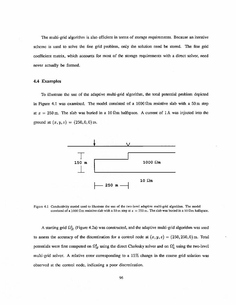
The multi-grid algorithm is also efficient in terms of storage requirements. Because an iterative

scheme is used to solve the fine grid problem, only the solution need be stored. The fine grid

coefficient matrix, which accounts for most of the storage requirements with a direct solver, need

never actually be formed.

4.4 Examples

To illustrate the use of the adaptive multi-grid algorithm, the total potential problem depicted

in Figure 4.1 was examined. The model consisted of a 1000 fZm resistive slab with a 50 m step

at x = 250 m. The slab was buried in a 10 m halfspace. A current of 1 A was injected into the

ground at (x,y,z) = (250,0,0)m.

T150 m

I

Figure 4.1 Conductivity model used to illustrate the use of the two-level adaptive multi-grid algorithm. The modelconsisted of a 1000 fm resistive slab with a 50 m step at x = 250 m. The slab was buried in a 10 m halfspace.

A starting grid (Figure 4.2a) was constructed, and the adaptive multi-grid algorithm was used

to assess the accuracy of the discretization for a control node at (x, y, z) = (250, 250,0) m. Total

potentials were first computed on fl using the direct Cholesky solver and on using the two-level

multi-grid solver. A relative error corresponding to a 15% change in the coarse grid solution was

observed at the control node, indicating a poor discretization.

1000 Qm

H— 250 m —H10 Qm

96

Depth

(m)

Depth

(m)

Ui

0 CD 0

Depth

(m)

0 0

1.11

CDCD

CD CD

,i-

CD -I _C

D

0 0

\CO

Di

U 0 0<— Di 0 p CD O

H

-iCD

8 oq

0 0

H 0 CD

Ui

0 0 0

Depth

(m)

0

(ii

0o

I0

•H

o0

00 0 0

to C,,

Ct

00

S

H 0 0 0

to In (-i

Di 00

H 0 0 0 0

H 0 0 0 0

to H-

Cc,

çt cv 00

S

H 0 0 0 0

a-

I-

-I

—----

-

I

0 0 0 0

to H 0, (-I

ci)00

S

H 0 0 0 0

-I

::z

!‘

0

C)

The error contribution map for the initial grid pair is shown in Figure 4.2a. Grey regions of the

error contribution map correspond to error contributions greater than a specified tolerance . was

chosen such that the sum of the error contributions greater than accounted for 90% of the relative

error at the control node. A partial grid refinement based on an examination of the error contribution

map was used to generate (Figure 4.2b), resulting in a new relative error of 4%. The largest error

contributions in this case are clearly associated with the current electrode and the corners in the model.

The second refinement resulted in the grid in Figure 4.2c. A relative error of 2% was observed, with

the largest error contributions associated with the coarse part of the grid between x = —500 m and

x = —125 m, as well as the region around the corners in the model. A third refinement resulted in

the grid shown in Figure 4.2d. Less than a 1% change was observed between the coarse and fine

grid solutions. Examination of the error contribution map (Figure 4.2d) indicated that if a further

reduction of the relative error was desired, refinement of the entire grid would be necessary. Profiles

of the coarse grid solutions for each grid refinement are shown in Figure 4.3. The modeled potentials,

particularly over the resistive ledge, are seen to change substantially as the grid evolves.

>

0

Ca,00

0

0I—

X position (m)

Figure 4.3 Profiles of the total potentials computed for the sequence of four grids generated in the first example.

—800 —400 0 400 800

98

18

16

14

10

0

4

2

4.0

Figure 4.4 Relative error computed at the control node for each of iteration of the adaptive solution of the problem inFigure 4.2. (a) ej plotted against iteration number. (b) e[ plotted against iteration number tothe power of —1.3. The dashed line shows the curve extrapolated to the origin.

Knowing how e changes with grid spacing allows the magnitude of the numerical error on

the final grid to be estimated. Note that if the numerical error is O(h1), then u = ‘uh + chm and

u = UH + c2h. The relative error = ilj, — UH = ch1(2 — 1) is also found to be O(h1). The

error on the fine grid solution is then given by

U— U= 2—

(4.24)

For this example, plots of the relative error as a function of iteration number (Figures 4.4a and 4.4b)

indicate an O(h’3)relative error. (4.24) gives an error on the final fine grid of about 1%. Note that

if the solution on f2 had been accepted as the final result, an error at the control node of about

26% would have resulted. The need to assess the error in the numerical solution, and the subsequent

need to refine the numerical grid, is apparent.

a. 0.0012

0.0010

>

0.0008

w 0.0006>

0

c 0.0004

0.0002

1.0 2.0 3.0Iteration number

0.00000.0 0.4 0.8 1.2

(Iteration number)13

99

As a second example, the secondary potential problem depicted in Figure 4.5 was examined. This

is the same problem used to illustrate the N-level multi-grid and multi-level algorithms developed

in Chapter 3. The adaptive multi-grid algorithm was used to generate the sequence of grids shown

in Figure 4.6a-d.

10002m

150 m1000 Qm

102m

250 m —i

Figure 4.5 Two resistive prism problem. The model for this problem consists of a pair of

1000 c2m resistive prisms in a 10 i2m halfspace.

The main contribution to the relative error in this case is seen to come from the point where the

two prisms meet. This point is known to correspond to a severe singularity in the potential gradient,

as discussed earlier. The result is a solution which changes considerably as the solution is refined

(Figure 4.7). Plots of the relative error as a function of iteration number (Figure 4.8) indicate an

O(h°55) relative error. This low order results in slow convergence of the numerical solution to the

final solution. Despite this poor convergence rate, the potentials will achieve a limiting value as

the mesh spacing approaches zero, as indicated by Figure 4.8. A limiting value of 3.45 mV for the

solution at the control node was estimated using (4.24).

100

U,

0 0 0

U,

0D

epth

(m)

oI

0I-

.0

00

0 0 0

‘-4

T1 4.

,4o.

C

‘<

0 0 0 0

ci I-’

rt

U,

I.fl

00

Depth

(m)

00

00

0 0 0

Dep

th(r

n)0

0 0 0

ci In rt

I-.

0 0 0 0

ci I-.

(0 r1 1”

I-.

0 0 0 0

0 0 0 0

ci I-.

In C) CD

0 0 0 0 0 0C-)

>

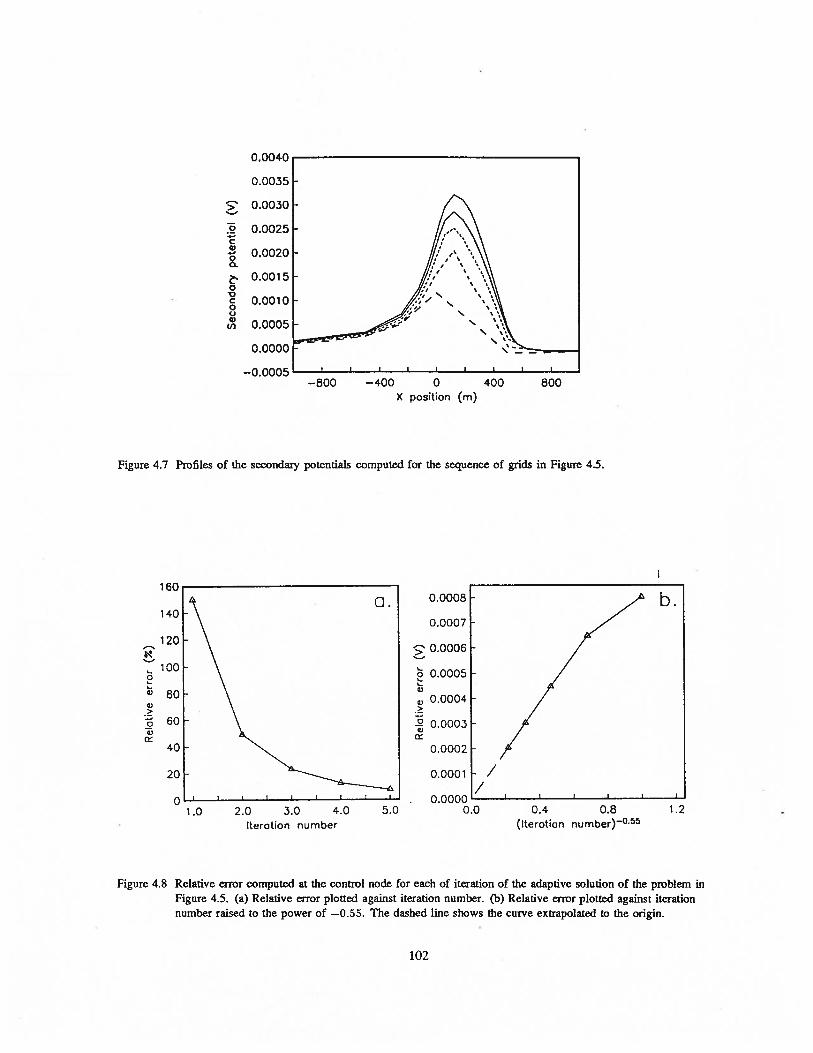
0

Ca00.

0

C00a

Figure 4.8 Relative error computed at the control node for each of iteration of the adaptive solution of the problem inFigure 4.5. (a) Relative error plotted against iteration number. (b) Relative error plotted against iterationnumber raised to the power of —0.5.5. The dashed line shows the curve extrapolated to the origin.

0.0040

0.0035

0.0030

0.0025

0.0020

0.0015

0.0010

0.0005

0.0000

—0.0005

X posftion (m)

Figure 4.7 Profiles of the secondary potentials computed for the sequence of grids in Figure 4.5.

1 60

1 40

—800 —400 0 400 800

a.

0

a)a>

Ca)

120

100

80

60

40

20

0

0.0008

0,0007

0.000 6

0.0005L

a, 0.0004>

0.0002

0.0001

• 0.0000 -

5.0 0.0

b.

I I

1.0 2.0 3.0 4.0Iterotion number

//

0.4 0.8(IterotJon number)”°’55

1.2

102

As a final example, the secondary potential problem depicted in Figure 4.9 was examined. The

model for this example was identical to the previous one, except that the resistivities of the prisms

were 0.1 1m. The sequence of grids generated by the adaptive multi-grid algorithm is shown in

Figure 4.lOa-c. Profiles of the coarse grid solutions for each grid refinement are shown in Figure

4.11. A relative error of less than 0.1 % after the second grid refinement indicates that the numerical

solution is extremely accurate in this case (Figure 4.12).

4*

T 0.112m

150 in0.1Qm

10 Qm

250 in -H

Figure 4.9 Model used in the third two-level adaptive multi-grid example. The model was identical to the one inthe second example (Figure 4.5), except that the resistivities of the prisms were 0.1 2m.

The results of these three examples illustrate how dependent on the model geometry the numerical

error is, and clearly show the importance of assessing the accuracy of the discretization for the

specific model at hand.

103

0.0a.

.1J0.a,

500.0

—1000.0 1000.0

0.0b.

E

0.a,

500.0

—1000.0 1000.0

0.0C.

E

4)0.a)0

500.0

—1000.0 1000.0

Figure 4.10 Sequence of three coarse grids generated by the adaptive multi-grid algorithm for the model in Figure 4.9.

0.0

Distance (m)

0.0

Distance (m)

0.0

Distance (m)

104

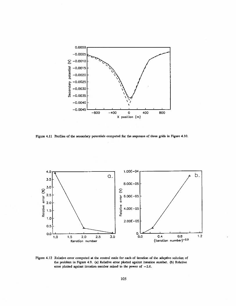
0.0000

—0.0005

—0.0010

—0.0015

—0.0020

. —0.0025

—0.0030

—0.0035

—0.0040

—0.0045—800 —400 0

X position (m)400 800

Figure 4.11 Profiles of the secondary potentials computed for the sequence of three grids in Figure 4.10.

Figure 4.12 Relative error computed at the control node for each of iteration of the adaptive solution ofthe problem in Figure 4.9. (a) Relative error plotted against iteration number. (b) Relativeerror plotted against iteration number raised to the power of —2.0.

‘-I

I I

—

I

0

Ii)>

00

1 ,00E—04

8,00E—05

6.OOE—05

4.OOE—05

2.OOE—05

>

I0I..

0

0>

00

b.

0. I

0.0 0.4 0.8 1 .2(Iteration number)2°

1.0 1.5 2.0 2.5Iteration number

3.0

105

4.5 Conclusions

Little work has been done to assess the accuracy of numerical techniques that are used regularly

to solve forward modeling problems in geophysics. It is generally assumed that if a numerical

algorithm performs well on simple models, where the solution can be generated analytically, it will

achieve comparable accuracy on more general problems. This chapter clearly shows this not to be

the case. In particular, corners and junctures are known to lead to singularities in the solution, which

in turn can lead to large errors in the numerical approximation. Because of the need to model DC

resistivity data over intruded and faulted regions, the influence of these features on the numerical

results cannot be ignored.

The magnitude of numerical errors that result from a poor discretization depends on the model,

as well as on the location of any current electrode sources, and is thus highly problem dependent. For

the 2D DC resistivity problem, large errors in the solution were encountered for some of the models

examined. In other problems, with very similar model geometries, the solution was found to be quite

accurate. Although rules of thumb can be formulated for constructing accurate discretizations, it is

difficult to predict a priori what accuracy will be achieved. Hence the need for verifying the accuracy

of a discretization for the problem at hand.

The verification of a numerical solution for a general model can only be done by re-solving the

problem on a finer grid and observing how much the solution changes. This is not done on a regular

basis because of the additional expense involved. For a 2D problem, computing the fine grid solution

using a direct Cholesky solver leads to a 17-fold increase in the number of operations required, and a

9-fold increase in the memory requirements. An efficient algorithm for solving the fine grid problem

that makes use of a two-level multi-grid algorithm has been presented. Work expended in calculating

the coarse grid solution is used in the multi-grid iteration to significantly reduce the effort required

to solve the problem on the fine grid. A modest two-fold increase in the number of operations is

then realized for large problems. Since the multi-grid algorithm makes use of an iterative procedure

106

on the fine grid, there is also very little additional storage requirements.

In some cases, the comparison of coarse and fine grid solutions to verify the accuracy of the

solution will indicate a large discretization error for the initial grid. In order to obtain a more accurate

solution in these cases, an adaptive grid refinement procedure was developed. This refinement

procedure is based on the contribution from the discretization error at each part of the grid to the

error at a particular control node. In most cases a sequence of two or three grid refinements was

found to be sufficient to achieve an acceptable solution. For problems involving strong singularities,

however, convergence to the final solution was found to be quite slow. In these cases, a large

number of refinements can be avoided by determining the order of the relative error. This establishes

a relationship between the relative error and the error on the fine grid solution, allowing the final

solution to be estimated.

107

Chapter 5

Numerical calculation of sensitivities

5.1 Introduction

A fundamental step in the solution of most non-linear inverse problems is to establish a

relationship between changes in a proposed model and resulting changes in the forward modeled

data. Once this relationship has been established, it becomes possible to refine an initial model to

obtain an improved fit to the observed data. In a linearized analysis the Fréchet derivative is the

connecting link between changes in the model and changes in the data. In some simple cases an

analytic expression for the Fréchet derivative may be derived. For more complicated problems where

it is not possible to obtain an expression for the Fréchet derivative, it is necessary to parameterize

the model and numerically solve for the sensitivities — i.e. the partial derivatives of the data with

respect to model parameters.

Literature in various fields illustrates how the sensitivities can be computed for specific problems.

However, there does not exist a detailed comparison of the approaches that are available for more

general problems. As such, when faced with solving an inverse problem, there is indecision about

what options exist and how best to formulate the sensitivity problem. Questions of accuracy and

computational efficiency also arise. The purpose of this work is to examine the various techniques

that are available, and to demonstrate their use in the calculation of sensitivities for the 1D DC

resistivity problem. Based on these results, an adjoint approach to the calculation of sensitivities for

108

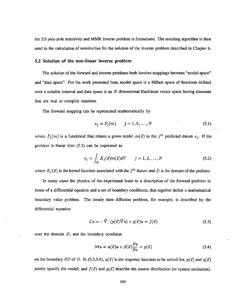
the 2D pole-pole resistivity and MMR inverse problem is formulated. The resulting algorithm is then

used in the calculation of sensitivities for the solution of the inverse problem described in Chapter 6.

5.2 Solution of the non-linear inverse problem

The solution of the forward and inverse problems both involve mappings between “model space”

and “data space”. For the work presented here, model space is a Hilbert space of functions defined

over a suitable interval and data space is an N dimensional Euclidean vector space having elements

that are real or complex numbers.

The forward mapping can be represented mathematically by

e3 =Fj(m) j 1,2,...,N (5.1)

where Fj(m) is a functional that relates a given model m() to the j’ predicted datum e. If the

problem is linear then (5.1) can be expressed as

e = fI(()m()dV j = 1,2,.. .,N (5.2)

where I( () is the kernel function associated with the th datum and B is the domain of the problem.

In many cases the physics of the experiment leads to a description of the forward problem in

terms of a differential equation and a set of boundary conditions, that together define a mathematical

boundary value problem. The steady state diffusion problem, for example, is described by the

differential equation

Lu = —f. (p(u) + q()ti = f() (5.3)

over the domain D, and the boundary condition

Mu = c(i)u + (ã) = g() (5.4)

on the boundary UD of D. In (5.3,5.4), u() is the response function to be solved for, p(s) and q()

jointly specify the model, and f() and g() describe the source distribution (or system excitation).

109

Although for simple geometries it may be possiNe to find a closed form solution to (5.3,5.4), it is

generally necessary to solve these numerically.

In the inverse problem, a model m* () is sought such that

ers = Fj(m*) j = 1,2,.. .,N (5.5)

where e is the th observed datum. If the forward problem is linear then a variety of standard

techniques can be used to solve the set of equations in (5.5) for m*() (e.g. Parker 197Th, Menke

1984, Oldenburg 1984); the particular technique used defines the inverse mapping. Although non-

iterative inverse mappings can be found for non-linear problems (e.g. Gel’fand-Levitan approaches

for inverse scattering problems), the techniques are often unstable in the presence of noise. Also,

for many non-linear problems encountered in geophysics, no direct inverse mapping has been found.

The usual strategy in these cases is to start with an estimated solution, mest(), and to solve the

forward problem to obtain the predicted data. A perturbation Sm(s) is then sought which, when

added to mest (i), yields a model that better reproduces the observed data. The procedure is repeated

until an acceptable fit to the data is achieved.

To derive equations that accomplish this, the th observation can be written in terms of the

expansion

= Fj(mest) + Fj’(mest)6m + 2)(mest)6m2 +... (5.6)

where the operator Fj’°(m) is the th order Fréchet derivative ofF3(m) (Griffel 1981, Zeidler 1985).

The first order derivative Fj’ (m) is referred to simply as the Fréchet derivative.

Letting 5e =— Fj(mes) be the misfit for the jul? observation, then (5.6) can be written as

6e =Fj1(mesi)6m + O(IIomII2) (5.7)

If the higher order terms represented by O(l6mI(2)are neglected, then (5.7) can be written as

6e ID mt)Sm()dV (5.8)

110

where Kj(, rn) is the Frdchet kernel associated with the jf!l observation. It is this kernel that estab

lishes the relationship between a small (first order) perturbation in the model and the corresponding

change in the datum. Since (5.8) is linear, the perturbation m() can be readily computed using stan

dard techniques once an analytic expression for the Fréchet kernel has been derived. General methods

for obtaining closed form expressions for the Fréchet derivative, with applications to the solution of

the 1D DC resistivity problem, are presented by McGillivray and Oldenburg (1990). Unfortunately,

with most problems of interest it is not possible to implement these techniques and one is forced to

appeal to numerical procedures. In these cases the inverse problem must be re-fonnulated and solved

using non-linear iterative methods for a set of unknowns that describe the model parametrically.

5.3 Solution of the non-linear parametric inverse problem

In a parametric formulation of the inverse problem, the model is written as

m() = mkk(x) (5.9)

where {kQ)} is a set of basis functions. The choice of basis functions determines the form of

parameterization to be used. For example, the domain D can be divided into subdomains Dk with

the kth basis function defined to be unity over the kth subdomain and zero elsewhere. The kth

parameter rnj is then the value of the model over the corresponding subdomain. Another approach

is to define a grid of nodes over D and to let the kth parameter be the value of m() at the location

of the kthl node. {bk} is determined by the interpolation method used to define the model between

nodes. A third possibility is to choose {l’k} as a set of regional basis functions (e.g. sinusoidal

functions used in a Fourier expansion).

Regardless of the parameterization selected, the model is completely specified in terms of the

vector n = (m1,m2,. . ., mM). The forward mapping is then represented by

e = Fj(ñ) j = 1,2 (5.10)

111

and the solution to the inverse problem is now the vector of parameters ni’ such that

j = l,2,...,i\ (5.11)

is satisfied.

As before, the relationship between the data and the model parameters is generally non-linear, and

an iterative approach must be used to solve (5.11) for ni. Numerous procedures for solving the non

linear parametric inverse problem are available, including the steepest descent, conjugate gradient and

quasi-Newton methods (Gill et al. 1981). These approaches make use of steepest descent directions

associated with a misfit objective function to iteratively improve some initial model estimate. The

perturbations are thus based on the sensitivity of an objective function to changes in the model

parameters. A standard procedure for solving non-linear parametric inverse problems that makes use

of sensitivities of each individual datum is the Gauss-Newton method (Gill et al. 1981). In this

formulation, the Taylor series expansion

M _ MM

= I(ñlest) + t)6mk + 6mkrnj +... (5.12)k1 k=1 1=1

is considered, where &Fj(i’ñ)/amkaml is the n’ order sensitivity of Fj(ni) with respect to the

kth,ltl,... parameters. Equation (5.12) can also be written as

cobs= (est) + + O(II6Ij2) (5.13)

Neglecting the higher order terms encompassed by O(njj2)yields the linearized equations

e= J6n. (5.14)

where J is the N x M Jacobian matrix whose elements J3,, = ôFj /Dmi, are the first order sensitivities.

It is clear therefore that the calculation of sensitivities is of fundamental importance to the solution

of the non-linear inverse problem.

112

5.4 Calculation of Differential Sensitivities

Given that a parametric solution to the inverse problem is required, and that the forward problem

can be expressed as a boundary value problem, there are three ways to obtain the sensitivities. In

the first method the sensitivities are computed from their finite difference approximations. For each

sensitivity the corresponding parameter is slightly perturbed and the forward problem is re-solved.

In the second method, a new boundary value problem is derived for each of the sensitivities, and

the sensitivities are solved for directly. In the third, the sensitivities are computed using the solution

to an adjoint Green’s function problem. All three approaches will be investigated here. Particular

attention is paid to the comparison of accuracy and numerical requirements of the algorithms.

5.4.1 Perturbation approach

The most straightforward way to calculate the differential sensitivities is to approximate them

using the one sided finite difference fonnula

(ñ) (+&iik)-F(ffI)(515)

amk mk

The perturbed forward response Fj(nz+ ff’k) is obtained by re-solving the forward problem after the

kth parameter has been perturbed by an amount lmk. Since the model must be altered to compute

the perturbed responses, each sensitivity requires the solution of a completely new problem. As such,

this ‘brute force’ method is inefficient, but it can nevertheless yield useful results (e.g. Edwards et al.

1984). The technique is also useful in providing numerical checks for the more efficient approaches

that are presented below.

5.4.2 Sensitivity equation approach

In the sensitivity equation method a new forward problem is derived whose solution is the

desired sensitivity function k(). Problems that have been addressed using this approach include

113

the 2D magnetotelluric problem (Rodi 1976, Jupp and Vozoff 1975, Cerv and Pek 1981, Hohmann

and Raiche 1988), the 2D electromagnetic problem (Oristaglio and Worthington 1980) and computer

aided design problems (Brayton and Spence 1980). Vemuri et al. (1969), McElwee (1982) and

Townley and Wilson (1985) use the approach to address problems in groundwater flow.

To illustrate the technique we consider the steady state diffusion problem given in (5.3,5.4).

Taking p() to be the model, and assuming the parameterization

= (5.16)

yields

Lu = —. (pl1(u) + q()u = f(s) in D (5.17)

-. -.

cx(x)u + = 0 on (5.18)

Differentiating (5.17,5.18) with respect to pk and writing pk(i5) = au()/apk, yields the sensitivity

problem

Pk = — (()c) + q()y = (b(ã$)zt) in D (5.19)

a()yk + = 0 on (5.20)

To compute the sensitivities for a model p(s), the forward problem (5.3,5.4) is first solved to

obtain u() at all points in D. For each parameter pk the corresponding sensitivity problem must

then be solved to obtain cpk () which is then evaluated at each of the observation locations. Note

that the source term V . (bk()u) differs for each k, so that a total of M + 1 forward problems

must be solved to obtain all of the sensitivities.

Since the M sensitivity problems and the original forward problem differ only in terms of their

right hand sides, they can all be solved using the same numerical forward algorithm. Note that if

114

the same scheme is used to discretize both the left and right sides of the sensitivity problem, then

the computed sensitivities will be exact in the sense that they will exactly predict how the numerical

solution will change as the model is perturbed by some small amount. In this way the calculation of

the predicted data and the sensitivities is consistent. When inverting real field data, the applicability

of the sensitivities will depend only on the ability of the forward modeling algorithm to represent

the true earth structure.

Since the sensitivity problem and the forward problem are identical except for their respective

source terms, their numerical solution can be done very efficiently if a direct solver (e.g. Cholesky

factorization) is used in the forward code. In that case only a single coefficient matrix factorization

is required to solve all M + 1 forward problems. This represents a considerable saving over the

perturbation method which would require forming and factoring the coefficient matrix once for each

parameter in the problem.

The sensitivity equation method is easily extended to the calculation of other sensitivities. For

example, the directional sensitivity, a(), given by

y) = Zkk(x) (5.21)

where o is a unit vector in parameter space, can be computed by first multiplying (5.19,5.20) by ak

and then summing over k to obtain the new problem

=. (p()) + q() = in D (5.22)

a(i)ya + = 0 on (5.23)

The directional sensitivity may then be solved for directly. Directional sensitivities are useful for

determining an optimum model perturbation once a direction for the perturbation has been selected

(e.g. Townley and Wilson 1985).

115

The sensitivity equation method can also be extended to the calculation of higher order sensi

tivities. For example, differentiating (5.19) and (5.20) with respect to the new parameter P1 yields

the problem

= — (p(’Y’s’,x) + q(F)çokl = (&,(yi) + (i(Ty,) in D (5.24)

a(pk1 + 3(F)-1 = 0 on (5.25)

whose solution is the second order sensitivity function cc’k, () = 82 u()/Upk Opi. Since the right side

of (5.24) is a function of Yk and,

a total of M2 + M +1 forward problems must be solved to obtain

all of the second order sensitivities. Several parameter estimation schemes that make use of these

higher order sensitivities to achieve rapid convergence are available (e.g. Brayton and Spence 1980,

Gill et al. 1981). The use of second order sensitivities in the estimation of parameter uncertainty

has also been described (Townley and Wilson 1985).

Another possibility is to consider the finite model perturbation given by

(5.26)

where = s and is a unit vector in parameter space. The resulting change in the response

is given by the Taylor series expansion

u() + u() = u(s) + Ya()8 + 2(X) 2 + a3(X) +... (5.27)

where the j order directional sensitivity pi is found to satisfy

=. (p()c’ci) + q(ai = . in D (5.28)

a() + = 0 on OD (5.29)

116

The tracking sensitivity, given by

=

____

= ()+a2().5+3().52 +... (5.30)

can be computed by solving (5.28,5.29) recursively for the required directional sensitivities.

Note that once a sufficient number of derivatives in the direction has been computed, (5.30)

can be used to predict how u(ã) will vary as the length of the model perturbation is increased. This

radial exploration strategy fonns the basis of an optimization algorithm proposed by Tahim (1979). In

a more general optimization procedure it could be used to replace direct line searches, thus avoiding

the need to solve the forward problem repeatedly for models corresponding to different values of .s.

5.4.3 Adjoint equation approach

The third method for calculating sensitivities is based on the adjoint Green’s function concept

discussed earlier. Some problems to which the adjoint equation approach has been applied include the

seismic problem (Tarantola 1984, Chen 1985), the DC resistivity problem (Smith and Vozoff 1984),

the magnetotelluric problem (Weidelt 1975, Park 1987), the groundwater flow problem (Neuman

1980, Carrera and Neuman 1984, Sykes and Wilson 1984, Sykes et al. 1985, Townley and Wilson

1985), the reservoir evaluation problem (Carter et al. 1974), and various problems in computer aided

design (Director and Rohrer 1969, Branin 1973, Brayton and Spence 1980). An equivalent approach,

based on a reciprocity relationship for transmission networks, has also been described (Madden 1972,

Tripp et al. 1984).

As an illustration, consider again the steady state diffusion problem given in (5.3,5.4). Having

obtained the sensitivity problem in (5.19,5.20), we consider the problem

= (i— ) (5.31)

where C is an adjoint operator and G(’ ) is an adjoint Green s function

117

Multiplying (5.19) by G* and (5.31) by ‘k’ and subtracting yields the expression

G* S°k — (pkl.G = G*(k) —

6(1—

13) (5.32)

Integrating both sides of (5.32) over the domain I), and making use of the properties of the Dirac

delta function, yields

ID{G*C S’k — S0k1*G*idV

= IDG* (bku) dV — SL)k(Xj) (5.33)

If the operator £* and the adjoint boundary conditions are chosen such that

. f

J [GL Yk — Yk G*jdV = 0 (5.34)D

for all G* and Yk. then the sensitivity for an observation location lj is given by

Yk(Xj)= L G*

. (ku)dV (5.35)

In this case the adjoint problem that satisfies (5.34) is found to be

LG* = —V (p(1)VG*) + q(1)G*= 6(1

—

lj) in D (5.36)

a(1)G* + p(1)---— = 0 on (5.37)

To compute the sensitivities, (5.36) and (5.37) must be solved for each observation location lj.

The integration in (5.35) is then carried out for each parameter. Since the source term in (5.36)

differs for each observation location, a total of N + 1 forward problems must be solved, although

this can be done efficiently if a Cholesky or other factorization is used.

In some cases the sensitivity of an objective function is desired. For example, if a steepest

descent method is to be used to minimize the objective function

= — e]2 (5.38)

118

where e = Fj(ñ), then sensitivities of the form

ôTflk

=_2(ebS Cj)Yk(j) (5.39)

must be calculated. Although this could be done by solving for each k(j). a more practical method

can be arrived at by considering the modified adjoint problem

L*7= in D (5.40)

(.).*+/3(.)&Go 01) (5.41)

The objective function sensitivities can then be computed from

= f ? (bku)dV (5.42)Omk D

When working with second order diffusion-type equations like those describing the DC resistivity

problem, obtaining the appropriate adjoint problem is relatively straightforward and can usually be

done by inspection. For problems described by more complicated governing equations, the adjoint

problem can sometimes be more easily derived from the coupled first order equations upon which

the governing second order equation is based. An example of this approach is presented for the

frequency domain EM induction problem in Appendix A.

5.4.4 Example — Calculation of sensitivities for the 1D resistivity problem

To illustrate the numerical computation of sensitivities, consider the DC resistivity problem for

a 1D earth. The governing equations are

£q5=—‘•

(oc5) =Th(ã5—) (5.43)

0 (5.44)

119

and

x,y,z)IR_ = 0 (5.45)

where (x, y, z) is the potential due to a single current electrode located at = (0, 0, z), u(x, y, z)

is the subsurface conductivity and R = -/x2 + y2 + (z — z3)2. When the conductivity varies only

with depth, (5.43-5.45) can be written as

Lq5 = _-(r) — — = —6(r) 6(z — z) (5.46)

0) = 0 • (5.47)

r, z)Iz_ = 0 (5.48)

where r = /x2 + y2.

Symmetry suggests taking the Hankel transform of

(A, z)= f r(r, z)Jo(Ar)dr (5.49)

where Jo(Ar) is a Bessel function of the first kind of order 0. The transformed response h(A, z) =

A(A, z) can then be shown to satisfy the forward problem

d2h dh 2 Al—-—- + + A h

= 2ircr(z)6(z

— z) (5.50)

h(A,0) 0 (5.51)

= 0 (5.52)

1dc7 ldpwhere w(z) = —— — = —

dz pdz

120

To parameterize the problem, let m(z) = lnp(z) be the model and represent the earth by a

sequence of layers of constant conductivity. Then

w(z) = mk-bk(z) (5.53)

where

k(Z)= { 1 for zk < < z4 (5.54)

0 otherwise

and Zk is the depth to the top of the kth layer.

Before the problem of computing the sensitivities can be addressed, an efficient solution to the

forward problem must be available. To meet this need, a forward modeling algorithm based on a

propagator matrix formulation was developed.

Let the earth be represented by a sequence of ML layers of constant conductivity overlying a

halfspace. Within any of the layers or the halfspace the governing differential equation for the 1D

resistivity problem reduces to

— + A2h = 0 (5.55)dz

The general solution to (5.55) for the kth layer can be written as

h(A, z) = Uke_ k1Z) + Dke(1_z) (5.56)

and for the half space as

h(A,z) = DML+le)(zML_z) (5.57)

The U and D coefficients for the kthi layer are then solved for in terms of those for the k + lj layer.

This requires the continuity of the electric potential

h(A,zt) — h(A,z) = 0 (5.58)

121

and the conservation of charge relationship

fork=k8 (5.59)A dz A dz 1 0 otherwise

where k3 denotes the source index for the case of a buried electrode.

Substituting (5.56) into (5.58) and (5.59) leads to the propagator matrix expression

(.) =Ak(.’) +8k (5.60)

where

e”’ 0 1 1 rkk= o etk tk rk 1

and

— 2ak _kUk+1tk — , — (5.62)

k + k+1 Uk + k+1

The source vector is given by

( —)d

sk={41rc7k(_eACtk)fork=k (5.63)

0 otherwise

Combining the propagator matrix expressions for each layer yields

(Ui)= A1A2 . ( 0 ) + A1A2 . (5.64)D1

U1 and D1 can be related using the boundary condition at z = 0 which requires that h(A, z) satisfy

—- -—h (A, o) = —ui(Ui — D1)= { for surface electrode (565)

A dz 0 otherwise

The solution h(A, 0) = U1 + D1 is then obtained from (5.64) and (5.65).

For the calculation of the sensitivities, the model shown in Figure 5.la was used. The model

consists of a 100 clm conductive zone buried within a more resistive 1000 Qm half-space. The

interval between z = 0 m and z = 400 m was divided into 20 m thick layers and the log resistivities

of all but the first layer were taken to be parameters. The transformed potentials for different values

122

of A were computed using the propagator matrix algorithm. Those results are shown in Figure 5.lb.

The presence of the conductive zone is indicated by the anomalously low values of the transformed

potential.

1 0—i

nE

((1

>‘

>

U

C0

C)

180

160

140>

120

100

80

0 50 100 150 200 250 300 350 400Depth (m)

io— 10—6 iO io i0(m)

Figure 5.1 (a) Conductivty model used in the 1D resistivity example.potential h(,X, 0) computed for the model shown in (a)

(b) Transformed surface

The transformed potential for A 0.005, corresponding to the maximum anomaly in Figure

5.lb, was selected as the single datum. The differential sensitivities k(A,O) = ôh(A,0)/ômk for

this wavenumber were then computed using each of the three basic methods.

10-2

a.

b.

10—2 10—1 10°

123

E

>.

>

(IC

Cl)

20

115>

>.

>

(nCV

U)

5

00 100

0

400

300 400

20

115>

>‘

>

C0)

U)

10

5

00 100 300 400

Figure 5.2 Sensitivity as a function of depth for A = 0.005 computed using (a) the perturbation method, (b)the sensitivity equation method, and (c) the adjoint equation method.

First, making use of the perturbation approach and the approximation given in (5.15), the sensitiv

ities for each layer were computed using perturbations corresponding to increases in the conductivity

of 1.0%, 10.0% and 100.0%. The sensitivities were computed using different perturbations so that

the effect of perturbation size on the accuracy of the approximation could be examined. The results,

plotted as functions of depth, are shown in Figure 5.2a. As expected, the transformed potential is

found to be most sensitive to changes in the near surface conductivity, and a rapid decrease in sen

sitivity is observed at the top of the conductive zone. The shielding effect of the conductive layer is

0 100 200 300Depth (m)

200Depth (m)

200Depth (m)

124

also apparent, resulting in the transformed potential being insensitive to changes in the conductivity

below the layer. A comparison of the sensitivities obtained for the three different perturbation steps

indicates that this approach is reasonably accurate except when large perturbations are used. The

computational work involved, however, is great for problems that involve a large number of param

eters relative to the number of data available. For this example a total of 20 forward problems had

to be solved to obtain the sensitivities for only one datum.

The sensitivity equation formulation is obtained by substituting the model expansion (5.53) into

(5.50-5.52) and differentiating with respect to mk. This yields

d?yk dpk 2 — dk dh—-------+w(z)——+-\ k—dz dz dz dz (5 66)

= —[(z — zk_1) — 6(z —

0 (5.67)

= 0 (5.68)

The current source in the original problem must be replaced by two buried sources — one on either

side of the ktI layer. Although dh/dz is discontinuous at each of the layer boundaries, the right

hand side of (5.66) can still be evaluated by noting that

dh Idh

J ö(z — zi)—dz= J 6(z — z1) Li H(z —

Z1L

[1_H(z_zi)]]dz

dh dlz=L J (z—zi)dz+ f6(z_zi)dz

(569)

id/i dli=

.; L +

where H(z) is the Heaviside step function. Thus the source term on the right side of (5.66) can be

replaced by the equivalent source

dh 11db dli 1- z)- = 6(z -

+- L-j (5.70)

125

which is easily evaluated. The sensitivity function yk(A,z) is obtained by using the propagator

matrix algorithm to solve (5.66-5.68) for each layer. The sensitivity vs depth relationship is shown

in Figure 5.2b. A total of 20 forward problems again had to be solved to compute the sensitivities

for the one value of ?. Comparing Figures 5.2a and 5.2b it is found that the sensitivities computed

using this method correspond to those found by the perturbation approach for o/o —i 0.

To solve for the sensitivities using the adjoint equation approach, an adjoint operator and boundary

conditions satisfying (5.34) must be found. Multiplying the first tenn in (5.66) by G* and integrating

by parts yields

G-dz =(thkG*

— k-3_) : + /° YkddZ (5.71)

Similarly, for the second term

j Gwdz = YkGW0

- j Yk-dZ (5.72)

The appropriate adjoint problem is found to be

— d2G— (w(z)G*) + A2G* = (z) (5.73)

0 (5.74)

= 0 (5.75)

The sensitivity yk(A, 0) is then given by

Yk(A,0) = _JG*(A,z)[6(z_zk_l)_6(z_zk)]h(A,z)dz (5.76)0 dz

The integrand in (5.76) can be evaluated using expressions similar to (5.70).

The adjoint problem in (5.73-5.75) can also be solved (after some manipulation) using the

propagator matrix algorithm, although a simple relationship can be found that allows G*(., z) to be

126

calculated directly from h(A, z). Note that if a new function G* = G*p is defined, then G*(A, z)

is found to satisfy the same forward problem as h(A, z) except that the current source is scaled by

—AI/2ir. Since the original governing differential equation is linear, the Green’s function G*(A, z)

required in (5.76) can be related to h(A, z) by

G*(A,z) =— h(A,z)

(577)Al p(z)

Once the forward problem has been solved for h(A, z), then (5.77) is used to obtain G(A, z) and the

integrations in (5.76) are carried out to compute the sensitivities. The results, shown in Figure 5.2c,

are identical to those found using the sensitivity equation method. Only a single forward solution is

required to generate all of the sensitivities using this approach.

Although the perturbation, sensitivity equation and adjoint equation methods form a powerful

arsenal for solving parametric inverse problems, variations on these basic techniques are also useful.

In particular, tracking sensitivities allow one to explore model space along a particular direction

without having to solve a large number of forward problems. To compute the tracking sensitivities

for the transformed response h(A, 0), the directional sensitivity problems

d(c-’ / dh

d2 d— dz2 + w(z) + A2.. =

‘N d(5.78)

—‘ Z ak?,bk J p-1 n = 2,3,...\k=i /

(A,0) = 0 (5.79)

= 0 (5.80)

are solved recursively for ii = 1,. . ., N. The tracking sensitivity expansion

_______

1 2= = x)+ c2(A,O)8+ cr3(A,0)9 +.3 2 6 (5.81)

127

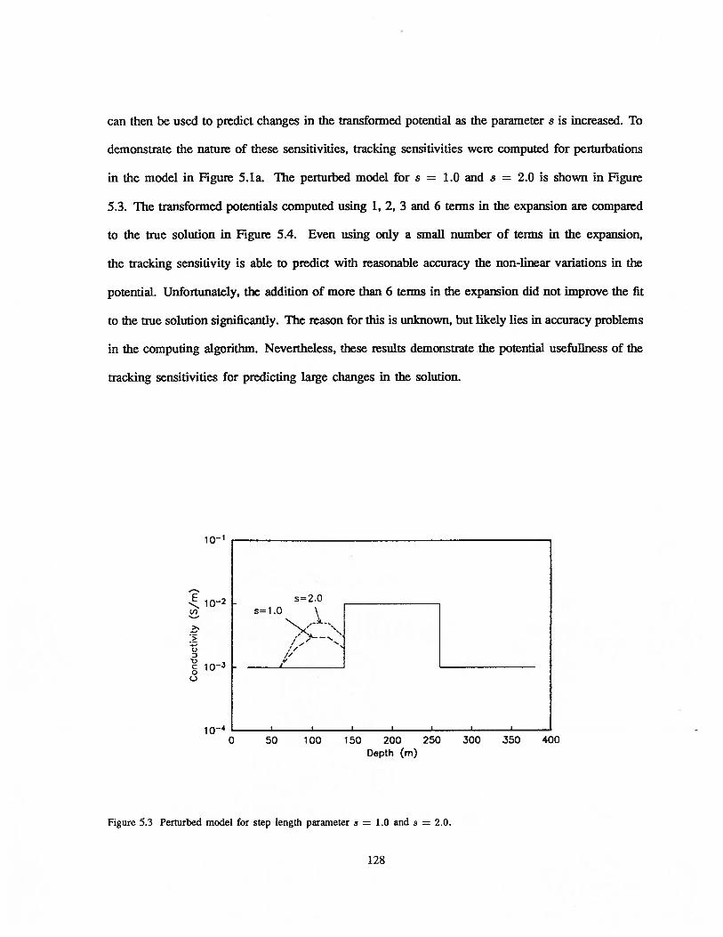
can then be used to predict changes in the transformed potential as the parameter s is increased. To

demonstrate the nature of these sensitivities, tracking sensitivities were computed for perturbations

in the model in Figure 5.la. The perturbed model for s = 1.0 and s = 2.0 is shown in Figure

5.3. The transformed potentials computed using 1, 2, 3 and 6 terms in the expansion are compared

to the true solution in Figure 5.4. Even using only a small number of terms in the expansion,

the tracking sensitivity is able to predict with reasonable accuracy the non-linear variations in the

potential. Unfortunately, the addition of more than 6 terms in the expansion did not improve the fit

to the true solution significantly. The reason for this is unknown, but likely lies in accuracy problems

in the computing algorithm. Nevertheless, these results demonstrate the potential usefuliness of the

tracking sensitivities for predicting large changes in the solution.

10-1

•-..- 10C’)

>‘

>

C,D

ic-3

iO0 50 100 150 200 250 300

Depth (m)

Figure 5.3 Perturbed model for step length parameter s = 10 and s = 2.0.

128

350 400

s=2.0s=1.0

E>

0

C

0a-

2.0s parameter

Figure 5.4 Transformed potential as a function of the step length parameter s computed using the tracking sensitivityapproach. The exact transformed potentials, calculated directly, are shown as a solid line.

5.5 Adjoint sensitivities for the 2D resistivity and MMR problem

The methods developed in the previous section can all be applied to the calculation of sensitivities

for the 2D resistivity and MMR inverse problems. Because of the size of the problems that are to

be solved, it is critical that the sensitivity calculations be done as efficiently as possible. For most of

the inverse problems that will be addressed, there will be considerably more parameters than data.

This avoids problems with convergence that often result from an overly restrictive parameterization.

For such underdetermined problems, the sensitivities are most efficiently calculated using an adjoint

equation approach. The use of a direct solver and an efficient inverse Fourier transform algorithm to

compute the various sensitivities can also be used to improve efficiency. The development of suitable

adjoint problems for the calculation of 2D resistivity and MMR sensitivities is presented below.

5.5.1 Choice of model and model parameterization

In formulating a solution to the inverse problem it is first necessary to define the model to be

recovered in the inversion. For most problems the conductivity u() is expected to vary over several

orders of magnitude. It will also be strictly positive. A natural choice is to consider the log resistivity

0.0 0.4 0.8 1.2 1.6

129

m() = — log (o)) = log (p(s)) as the quantity to be recovered. This imposes a natural positivity

constraint, and allows regions of high and low resistivity to be weighted equally in the inversion.

For the work been done here, the model is assumed to be two-dimensional, with variations

in material properties permitted only in the x and z directions. The model is parameterized by

representing the continuous 2D structure o(x, z) by a set of M rectangular prisms of constant

conductivity extending to infinity in the y direction. The continuous conductivity model is then

given by

u(x,z) = kk(x,z) (5.82)

where bk(x, z), the kth basis function, is unity across the kth prism and zero elsewhere. k and mk

are the conductivity and log resistivity of the ktI prism. This parameterization scheme is consistent

with the assumptions made in the forward modeling algorithm developed in Chapter 2.

5.5.2 Calculation of 2D pole-pole sensitivities

Making use of the adjoint equation approach, the expansion of the model in terms of the basis

functions (5.82) is substituted into the governing equation and boundary conditions for the transformed

pole-pole potential problem, given in (2.7-2.9). Differentiating with respect to Uk yields the sensitivity

problem

_() +kk_L(Uk) = (k) _kk+(k) (5.83)

Pk(X,k,0) 0 (5.84)

on ODøo (5.85)

where [)D corresponds to the left, right and bottom boundaries of the grid, and k(x, 1c, z) =

9k(x, k, z) is the desired sensitivity in the transform domain.

130

To compute the sensitivity at (x0b3,Yobs, Zobs) an adjoint operator and boundary conditions that

satisfy (5.34) must be obtained. For the sensitivity problem in (5.83-5.85), the appropriate adjoint

problem is

—- (u) + kuG* —

(*)= 6(x

— 2-obs, Z — (5.86)

—G (x,k,O)=O (5.87)

on (5.88)

Since the form of (5.86-5.88) is identical to that of the original tranformed forward problem, the same

finite difference algorithm can be used to solve both problems. Full advantage can then be taken of

the computational savings associated with decomposing the original coefficient matrix.

Note that for the resistivity problem it will often be the case that an electrode used to make one

or more potential measurements will have also been used at some point in the survey as a current

electrode. If this occurs, then (5.86-5.88) need not be solved since G(x, k, z, Zobs, Z0b3) can always

be computed directly from the forward modeled response qS(x, k, z) due to the current electrode

at (xobs,zobs).

Once the adjoint Green’s function has been obtained, the sensitivity of the corresponding

transformed potential can be computed from

- at 2 -

YkQobs, k, Z0b)= JD

—

(5.89)

The sanie procedure for discretizing the original forward problem must be used to evaluate the

integral in (5.89). This ensures that the sensitivities are exact for the given forward modeled solution.

131

Assuming the ij element in the forward problem corresponds to the kth parameter, the discrete

form for (5.89) is given by

k2pk(Xobs, k,z0b3) = —- + G÷1,1q1i,,+

G+1,1+i+

Liz, (:+i,—

ix (i,j+1 —

2x+

2zj

—

+Ixi

— (5.90)+ i+1,j 2zz 2z

—

£x—+G1

2x+

2Lzj

— i+1,j+1) (+ —

2x 2z1

Once the transformed sensitivities have been computed, an inverse Fourier cosine transform is

required to obtain the sensitivies in the spatial domain. This is given by

Yk(Xobs, Yobs, Zob3) = j k(Xobs, k,z0b5)cos (ky0b5)dk (5.91)

Taking the model to be the logarithm of the resistivity, the sensitivity of the kth model parameter

is then computed from

(Xobs, Yobs,z0bs) = kYk(Xobs, Yobs, Zobs) (5.92)ãmk

132

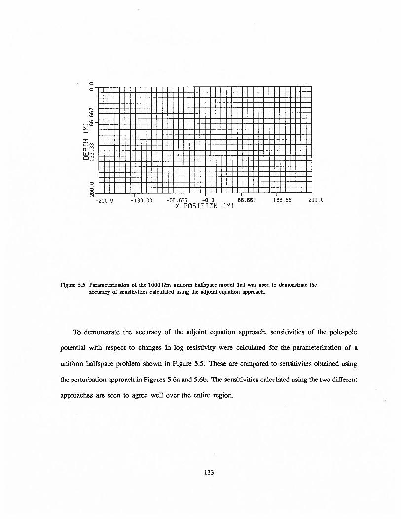
)0 .0

Figure 5.5 Parameterization of the 1000 Qm uniform halfspace model that was used to demonstrate theaccuracy of sensitivities calculated using the adjoint equation approach.

To demonstrate the accuracy of the adjoint equation approach, sensitivities of the pole-pole

potential with respect to changes in log resistivity were calculated for the parameterization of a

uniform halfspace problem shown in Figure 5.5. These are compared to sensitivites obtained using

the perturbation approach in Figures 5.6a and 5.6b. The sensitivities calculated using the two different

approaches are seen to agree well over the entire region.

CDCD

CDCD

(V)

-65.667 -0.0X POSITION (M)

133

c,Q C

)C

..,•

CD

Q

N)

C C C>

CD

CD

8.

5— U

)°

U)

U)

U)

II. CD

CD.

><cn 0

,C)

lD-j

0’—

C

0 (I)

C—

—

—4

)

E.

a,o

0’ a,

(D

CCD

a,C)

0o

CD‘

U)

U)

U)

U)

II—

‘0C

D CN

)o

-iC C C

CD.

DEP

TH(M

)133.3

366.6

67

0.0

N)

C C b U)

U)

U)

0)

0,

0•)

0,

-D-J

0 U’,

H)

—C

00 0

,0

, a) a)

5.5.3 CaLculation of 2D MMR sensitivities

Since the transformed magnetic field components are linear functions of the modeled potentials,

an adjoint approach can be formulated for the calculation of the magnetic field sensitivities. Consider,

for example, the transformed x component of the magnetic field, given by

E(x,k,z) =.— j f dx’dz’ (5.93)

where r’ = — x’)2 + (z — z’)2. Substituting the model expansion (5.82) into (5.93) and

differentiating with respect to k yields

——E(x,k,z)= _.Jf

_

ky[k(x’,ky,z’)—-c(x’,z’)—_ Z (5.94)

+(x’, k, z’) (x’, z’)] 1 (kr’) dx’dz’

Evaluation of the term

tl =—

f00f dx’dz’ (5.95)

is straightforward since will be known throughout the domain once the forward problem has been

solved. Exactly the same algorithm that is used to carry out the integration in (5.93) can be used to

evaluate ti. Less straightforward is the evaluation of the term

0000

=

— j j dx’dz’ (5.96)

To evaluate t2 directly, k must be computed throughout the domain, requiring the solution of a

forward problem for each parameter. For the underdetermined inverse problem, it would be better

to formulate an adjoint problem whose solution allows t2 to be computed without having to solve a

large number of additional forward problems.

Assuming a linear variation of k along each cell edge, t2 is given by

= JLOky(cxj,

—u,1)[()i J (x

—

x’)i=1 j=1 (5.97)

.KO(k7.6)dx’ + f (x’—

xi) Ko(kYrb5)dx’]

135

where rOb3 = \/(Xobs — x’) + (Zobs — z)2. Now consider the adjoint problem

OIOG*N2 * Of OG——(cT--——I+kgG——u—--—

Ox\ Oxj Oz\ OzN—1 N, rpok v—’ i6(xx,zzi)

— L1 (c7ij—oij_i)I2ir

i=1=1 I (5.98)

•

[+1

(x.1— x’)Ko(kyr5,)dx’ +

6(x — xj1,Z — zj)

xi+1

f (x’— x)Ko(kYrbS,)dx’]

subject to

_G*(x,k,O) = 0 (5.99)

G*(x,ky,z)+aG*(x,ky,z)=0 Ofl OD (5.100)

Multiplying (5.98) by ck and (5.83) by G*, subtracting the results and integrating over the domain

yields

t2= L i: [ (k) — kbk+

- (5.101)

()] G(x, k, Z Z0b3,zobs) dx dz

Note that this is identical to the integral in (5.89) that must be evaluated when computing k by the

adjoint Green’s function approach — only the Green’s function has changed. The same scheme used

to numerically evaluate (5.89) is also used to evaluate (5.101). The calculation of the sensitivities

for the y and z components of the transformed magnetic fields are carried out in a similar manner.

To illustrate the accuracy of the magnetic field sensitivity calculations, sensitivities of the y

component of the magnetic field were computed using the adjoint approach for the uniform halfspace

problem in Figure 5.5. These are compared to those obtained using the perturbation approach in

Figures 5.7a and 5.Th. Again, the sensitivities calculated using the two approaches agree well over

the entire region.

136

a.

200.0

200 0

Figure 5.7 Sensitivities computed for the By response from an MMR experiment for the 1000 lm uniformhalfspace problem shown in Figure 5.5. a) Sensitivities of the MMR response computed usingthe adjoint equation approach for a current electrode at = (—100, 0,0) m and a magneticfield measurement at = (100, 0,0) m. b) Sensitivities computed using the perturbationapproach. A perturbation of 1% in the conductivity was used in the calculation.

CD

CD.—CD

I— C)

LU 0’

cD2

-200.0 -133.33 -66.667 -0.0 66.667 133.33X POSITION IM)

b.

I—CDCD

CD— CD

II— (‘

CLmLUcD0’

-66.67 -0.0X POSITION IM)

137

5.6 Conclusions

Although numerous procedures are available for the solution of the parametric inverse problem,

the choice of procedure is often limited by the size of the problem at hand. Clearly, the size of the

problem will restrict the number of forward solutions that can reasonably be carried Out through the

course of an inversion. This will in turn limit the types of sensitivities that can be computed. The

calculation of higher order data sensitivities, for example, will generally be impractical because of the

number of forward problems that must be solved. This usually rules out the use of the second-order

Newton optimization procedure for all but the simplest of problems. For 2D problems, and smaller

3D problems it may be feasible to compute the first order data sensitivities required for Gauss-Newton

optimization. In these cases, the use of a sensitivity equation approach for overdetermined problems

and the adjoint equation approach for underdetermined problems will minimize the number of forward

solutions that are required. The use of a perturbation approach is almost always impractical because

of the need to form and decompose a new finite difference coefficient matrix for each forward

solution. For truely large-scale inverse problems it may be computationally practical to solve only

a few forward problems. In these cases it may be necessary to solve for the sensitivities of a data

misfit objective function, in which case a modified adjoint approach can often be used to minimize

the number of forward solutions. For problems where only objective function sensitivities can be

computed, a steepest descent or conjugate gradient approach can be used in the inversion.

For the 2D inversion of DC resistivity and MMR data it was found feasible to solve for

sensitivities of each datum, thus permitting the use of an optimization procedure based on the Gauss-

Newton approach. Since in most cases considerably more parameters than data will be used in the

solution of the inverse problem, an adjoint equation approach was employed. The use of a direct solver

for the forward modeling algorithm, and the use of an efficient inverse Fourier transform scheme

permitted the rapid calculation of the sensitivities. The computed sensitivities were found to be exact

in the sense that they exactly predicted the changes in the numerical solution for small changes in

138

the model parameters. A comparison of the numerically computed sensitivities to those computed

using the perturbation approach was used to verify this accuracy. Further examples illustrating

the calculation of the 2D sensitivities and a comparison to analytic solutions for a halfspace are

presented in McGillivray and Oldenburg (1990). The successful use of these numerically calculated

sensitivities in the inversion of DC resistivity and MMR data, presented in Chapter 6, further verified

their accuracy.

139

Chapter 6

Subspace Inversion of DC Resistivity and MMR Data

6.1 Introduction

Early work on the inversion of DC resistivity data was devoted almost exclusively to the 1D

problem (eg. Pekeris 1940, Zohdy 1965, Koefoed 1966, Inman et al. 1973, Inman 1975, Oldenburg

1978). In recent years, however, the focus has shifted towards the solution of the multi-dimensional

inverse problem (Vozoff 1960, Pelton et al. 1978, Petrick Ct al. 1981, Smith and Vozoff 1984,

Tripp et al. 1984, Sasaki 1989, Sasaki 1990, Sezenger 1990, Park and Van 1991). Because of

the complexity of these higher dimensional problems, parametric inverse techniques have been used

almost exclusively.

Many recent attempts to solve the parametric inverse problem have relied on a coarse param

eterization of the model to help stabilize the inversion. The form of this parameterization (i.e. the

number and geometry of the parameter elements) is based ideally on available geological information

that might be available, but often is chosen as a matter of convenience to simplify the numerical

computations in the inversion. In many cases the regional model is specified before hand, and only

a small sub-region of the model is solved for in the inversion. In the absence of detailed geological

information either of these strategies involves considerable risk since the outcome of the inversion

will likely be influenced by the regional model and parameterization scheme used. As well, the lack

140

of flexibility in the solution that results from a coarse parameterization can lead to poor convergence

(or even divergence) of the model iterates.

These problems can be avoided by using a large number of parameters to represent the model.

This gives the inversion algorithm more flexibility, and makes the outcome of the inversion less

sensitive to the form of the parameterization. Unfortunately, the use of a large number of parameters

in an inversion can also lead to serious problems with non-uniqueness.

An approach for inverting DC resistivity and MMR data that avoids these problems was the

focus of the work presented in this chapter. A strategy of solving for a large number of parameters

relative to the number of data was adopted. The minimization of a global norm of the model was used

to address problems with non-uniqueness and to drive the inversion towards an acceptable solution.

Procedures for making the inversion computationally feasible were also developed. The resulting

inversion algorithm was then tested by inverting a variety of synthetic DC resistivity and MMR data

sets. A set of E-SCAN field data for a prospect in Nevada was also inverted.

6.2 Generalized subspace inversion

In order to achieve a reliable result when detailed geological information is not available, the

parameterization must be fIne enough to yield a solution that is independent of the parameterization.

At the same time, solution space must be restricted enough so that the inversion is both stable and

computationally practical. The strategy that has been adopted in this work is to make use of as fine

a parameterization of the model as possible. Parameterizations that result in a thousand unknowns

for the 2D problem are typical. In order to deal with problems of non-uniqueness that arise from the

use of such a large number of parameters, a global model objective function is also minimized. A

reformulation of the least-squares procedure based on a generalized subspace approach has also been

developed to deal with the computational problems associated with inverting for a large number of

unknowns. This involves a re-parameterization of the model perturbation in terms of a set of basis

141

vectors that are chosen in some responsible manner. The development of the generalized subspace

approach, and its application to the DC resistivity problem, is described below.

6.2.1 Non-linear least-squares approach

The generalized subspace approach is based on a reformulation of the non-linear least-squares

solution of the parametric inverse problem. The more familiar least-squares approach is obtained

through a minimization of the data misfit objective function, given by

= Iv’— e()5 = (ë COb)(e Cobs) (6.1)

where tobs and ë. are the observed and predicted data respectively. In this work it will be assumed

that the data have been normalized by their estimated standard deviations. Given an estimate of

the model nV’, a perturbed model n = n—1 + Lñi is sought that minimizes (n4 + ni).

Using the expansion

(fl_1 + tWt) = e(n’) + JL\ni (6.2)

yields the linearized approximation

11(nV’ + Ln) = (J — )T(j — ë’) (6.3)

where = — (n’). Minimizing (6.3) with respect to each Lmk yields the model

perturbation

= (JTJ)_lJT (6.4)

The least-squares update to the previous model estimate is then given by

= ff’’ + (JTJ)_lJTië (6.5)

142

A single iteration of the least-squares procedure involves computing the data misfits and sen

sitivities for the model from the previous iteration. The model is then updated using (6.5) and

the procedure is repeated until either an adequate fit to the data is achieved, or until no further

improvement is observed.

6.2.2 Minimization of a global model norm

Since there is usually insufficient information to uniquely resolve the entire parameter set, the

solution of the non-linear inverse problem using (6.5) is often unstable. This is characterized by the

singular, or nearly singular, nature of the matrix ,jT j that must be inverted to compute the perturbation

in (6.5). To control this instability, further constraints on the nature of the recovered solution must

be imposed. This can be accomplished by requiring that the model perturbation minimize the model

norm objective function

= iiwnii2= TWTW (6.6)

where W is a weighting matrix used to define the norm. Note that W must be invertible for IIWn

to be considered a true norm. In practice this will always be ensured. The perturbation is required

to satisfy the linearized data misfit constraint

= (J —

— e) = (6.7)

where is the final target misfit that is selected on the basis of the assumed observation errors.

Minimizing (6.6) subject to (6.7) yields the damped least-squares or Gauss-Newton update

= ñz1’ + (JTJ + ,tWTW)_lJT (6.8)

The ridge regression parameter p is selected so that the updated model computed from (6.8) satisfies

either the linearized misfit constraint (6.7) or the non-linear constraint

= (e(n’ + ñ) — eobs) (e(rn’ + n)— = (6.9)

143

Although computing the linearized data misfit does not involve any additional forward modeling, it

is not valid for large perturbations and must therefore be used with some care.

The use of (6.6) to control the nature of solution recovered in the inversion leads to a “creeping”

strategy, where only the norm of the model perturbation is minimized. In a “leaping” strategy, the

global norm of the model relative to a reference model ñiref is minimized. This is achieved by

minimizing the global model norm objective function

= lIW(nV’1+ zni— mref)U2 (6.10)

The corresponding Gauss-Newton update is then found to be

= n-1 + (JTJ + iLWTW)_lJT(Li+ WTW(ñ_l mref)) (6.11)

Minimizing a global model norm allows for the specification of a reference model in the model

objective function. Since the distance from this reference model will be minimized in the inversion,

it can be used to incorporate a priori imfonnation about the true earth. The use of a global model

norm also allows for unnecessary structure to be removed from the solution once the inversion has

achieved the desired level of misfit.

6.2.3 Computational aspects of the Gauss-Newton approach

The use of the traditional Gauss-Newton approach to solve for a large number of parameters

in an inversion can result in an excessively costly calculation, both in terms of execution time and

memory. To examine where the majority of the computer resources are actually used, consider the

parameterization shown in Figure 6.2. Let M and M2 be the number of cells in the x and z

directions respectively, and assume that the same mesh is used to discretize the forward problem and

parameterize the model for the inverse problem. The number of floating point operations and the

memory requirements for each of the basic steps in a Gauss-Newton iteration are given below.

144

Solution of the forward problem

The finite difference algorithm developed in Chapter 2 makes use of a Cholesky decomposition

to solve the DC resistivity forward problem. Since M > M for most problems, the nodes in the

numerical grid are assumed to be numbered by columns to minimize the bandwidth of the coefficient

matrix. For a large problem, with n,9 unique source locations, the computer resources required to

perform the Cholesky decomposition and to solve for the n right hand sides are given by

Nw = + n3 2MM flops2 (6.12)

Ns = entries

(Golub and Van Loan 1983, p. 96), where Nw is the number of floating point operations (flops)

required to obtain a solution and Ns is the number of non-zero entries that must be stored. For

large problems, a significant amount of work is clearly required to initially decompose the matrix.

Solutions for different source locations can then be computed relatively cheaply.

Calculation of the sensitivities

Once the coefficient matrix has been factored and stored, the forward modeling of the sensitivities

using the adjoint equation approach can be computed relatively cheaply. For a large problem, with

obs unique observation locations, the computer resources required are

Nw = n0 2MrM flops (6.13)

Inversion of the matrix (jTj + 11WTW)

The inversion of the matrix (JTJ +1tWTW) is carried out using the Golub-Reinsch singular

value decomposition routine (Golub and Van Loan 1983). i.e., (jTj + = RA_1RT.

The resources required to store the matrix and factor it are

6MM flops(6.14)

1Ts = MM entries

145

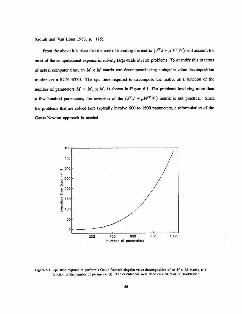
(Golub and Van Loan 1983, P. 175).

From the above it is clear that the cost of inverting the matrix (jTJ + pWT W) will account for

most of the computational expense in solving large-scale inverse problems. To quantify this in terms

of actual computer time, an M x M matrix was decomposed using a singular value decomposition

routine on a SUN 4/330. The cpu time required to decompose the matrix as a function of the

number of parameters M = Ma, x M is shown in Figure 6.1. For problems involving more than

a few hundred parameters, the inversion of the (JTJ + ILWTW) matrix is not practical. Since

the problems that are solved here typically involve 500 to 1500 parameters, a reformulation of the

Gauss-Newton approach is needed.

A (V

350

_,. 300

E250

0U

200E

0

U

x

150

100

50

0

1000

Figure 6.1 Cpu time required to perform a Golub-Reinsch singular value decomposition of an M x M matrix as afunction of the number of parameters M. The calculations were done on a SUN 41330 workstation.

200 400 600 800Number of parameters

146

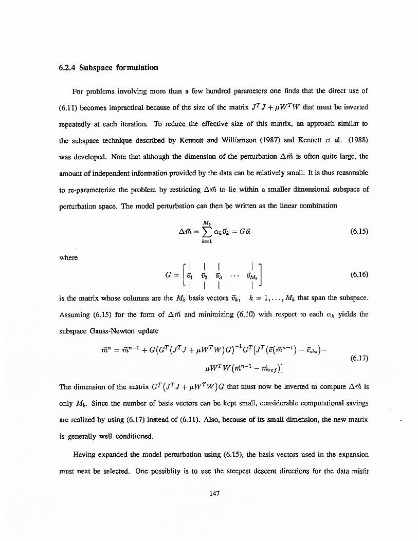
6.2.4 Subspace formulation

For problems involving more than a few hundred parameters one finds that the direct use of

(6.11) becomes impractical because of the size of the matrix jTj + ,uWTW that must be inverted

repeatedly at each iteration. To reduce the effective size of this matrix, an approach similar to

the subspace technique described by Kennett and Williamson (1987) and Kennett et al. (1988)

was developed. Note that although the dimension of the perturbation Lni is often quite large, the

amount of independent information provided by the data can be relatively small. It is thus reasonable

to re-parameterize the problem by restricting to lie within a smaller dimensional subspace of

perturbation space. The model perturbation can then be written as the linear combination

Mb

rn=akvk=Gc1 (615)

where

(6.16)

I Iis the matrix whose columns are the M5 basis vectors k, k = 1,. . . , M that span the subspace.

Assuming (6.15) for the form of iñi and minimizing (6.10) with respect to each k yields the

subspace Gauss-Newton update

fl = n-1 +G(GT(JTJ+WTW)G)GT[JT((il_1) —Ebs)—(6.17)

T47TW(ñi)l— ?Tl,.f)]

The dimension of the matrix GT (jTj + 11WTW) G that must now be inverted to compute ni is

only M&. Since the number of basis vectors can be kept small, considerable computational savings

are realized by using (6.17) instead of (6.11). Also, because of its small dimension, the new matrix

is generally well conditioned.

Having expanded the model perturbation using (6.15), the basis vectors used in the expansion

must next be selected. One possiblity is to use the steepest descent directions for the data misfit

147

and global model objective functions as basis vectors. For the data misfit term, a perturbation in the

steepest descent direction, Lni, satisfies the problem

minimize {IIW = jTWTW}

(6.18)

subject to 4)(nV—’ + n) = 4)(M’) + =

(e.g. Gill et al. 1981, p. 102). The solution to (6.18),

=

— 4)(n_1) —

(WTW)_l 4) (6.19)V4)T (WT W)-’ V 4)

defines the direction for the first basis vector. Substituting for 4) in (6.19) and ignoring scale factors,

yields the basis vector

= _(WTW)_1.= _2(WTW)_1JT(ë_ eobs) (6.20)

Note that the steepest descent direction used to obtain (6.20) has been defined with respect to the

same norm used in the global model objective function. Since the perturbation corresponding to

(6.20) will minimize this norm, the global model objective function will remain small through the

course of the inversion.

Similarly, the steepest descent direction for the global model objective function yields the second

basis vector

V2 _(TzVTy1T= ñirej) (6.21)

The basis vectors in (6.20) and (6.21) are equivalent to those used by Kennett and Williamson

(1987) in their initial subspace formulation.

6.2.5 Use of additional basis vectors — the generalized subspace approach

In formulating a solution to the DC resistivity inverse problem it was necessary to develop a

more general subspace algorithm that makes use of an expanded set of basis vectors (McGillivray

148

and Oldenburg 1991). Since the DC resistivity inverse problem is often very non-linear, serious

convergence problems can result from the use of an overly restrictive basis set. In the generalized

formulation, steepest descent directions corresponding to different subsets of the data are used to

define the basis set. Basis vectors that lead to accelerated convergence are also used to supplement

the basis set. Additional basis vectors are also selected so that unnecessary character can be removed

from the solution as the inversion progresses. This is particularly important in the solution of the DC

resistivity problem, where the localized nature of the pole-pole sensitivities often leads to artifacts

in the solution that are not required to fit the data.

The use of a large number of basis vectors in this generalized subspace approach can significantly

increase the cost of the inversion. Since the number of basis vectors included in the set must be kept

to a minimum, it is important that they be chosen with some care. The most important considerations

in selecting the basis vectors are that they be reasonably independent, and that they provide a rapid

decrease in either the data misfit or global model norm. Although there are many basis vectors that

meet these requirements, several were found to be particularly useful. These are described below.

Directions corresponding to sub-objective functions

In most cases a geophysical survey will consist of a set of distinct experiments, each involving

measurements made around a particular source location. In the pole-pole DC resistivity experiment,

for example, measuring the voltages due to a single current electrode would constitute a distinct

experiment. A common source gather is thus a natural way of grouping the data. This grouping leads

to a collection of sub-data sets that are spatially independent. It is also computationally convenient

to group the data in this manner since with forward modeling techniques like the finite difference

and finite element method, the responses due to each source excitation are modeled separately.

Using a common source grouping, a separate data misfit can be defined for each sub-data set.

149

i.e.

k(rn)

=

(e03, e,k)2 (6.22)

where k is the number of measurements made using the kill source, and and e,k are the

corresponding obsers’ed and predicted data respectively. The total misfit is given by

= k(rn) (6.23)

where n. is the number of sources used in the survey.

Having defined the data misfit functions {k, k = 1,.. . , n8} , a set of basis vectors can be

constructed from the corresponding gradient vectors {\k(ni), k = 1,. . ., n} . Thus the kth basis

vector is given by

t’k _(WTW)_’4k = _2(WTW) JT(ë— éobs,k) (6.24)

Since each 5k is a descent direction for a çb, the total data misfit 5 = cbj. will be sensitive to

model changes in any of the ‘ilk directions. As well, since each corresponds to a new source

location, the basis vectors will be reasonably independent.

If more basis vectors are desired, other data groupings are also possible. For example, the data

set can be further subdivided into near, middle and far offset measurements. These new basis vectors

should also be reasonably independent. The subdivision of the data set can be carried to its extreme,

with a basis vector being associated with each individual datum. However, since the data in the

complete data set display a certain amount of dependence, only a relatively small number of subsets

should be required.

Constant and linear basis vectors

Throughout the course of an inversion the Gauss-Newton algorithm will be attempting not only

to fit the data, but also to minimize a norm of the model. Once a fit to the data has been achieved,

150

the algorithm will then attempt to reduce the model norm by removing unnecessary structure from

the solution. Note, however, that since none of the basis vectors have energy where the data has low

sensitivity, the model cannot change in these regions even if it would lead to a significant reduction

in the global model norm. To allow the inversion to change the model in this region, it may be

necessary to supplement the set of basis vectors with additional vectors that have energy where the

data is insensitive. Possibilities include vectors corresponding to linear functions of depth, layers,

and rectangular rectangular cells. The form of these basis vectors can be based on a prior knowledge

of the true earth structure.

Basis vectors corresponding to the high frequency component of the model

Another way of allowing the algorithm to remove structure that has been built up in the model

is to include in the basis set the vector

Vk = (ift— rnref) — S(ifl — mref) (6.25)

where S is some smoothing operator. This new basis vector will be dominated by the high frequency

structures associated with the global model perturbation. By including this vector in the basis set,

the algorithm can be given the flexibility to remove high frequency components of the model that

are not required by the data. For a 2D problem with constant mesh spacing, a possible choice for

the matrix S is denoted by the stencil

1010S=— 1 4 1 (6.26)

8o 10

where the stencil represents the two-dimensional operator that is applied to the grid of model values.

Basis vectors corresponding to perturbations from previous iterations

In some cases the recovered model is found to oscillate between two different models as the

inversion approaches a fit to the data. The misfit is found to decrease for each pair of iterations, but

151

only slowly. This problem usually occurs when the weighting matrix used to smooth the sub-gradient

vectors results in basis vectors that are nearly parallel to the level lines of the misfit objective function.

A way of avoiding these oscillations, and to generally improve the convergence rate of the subspace

method, is to include perturbations from previous iterations in the basis set. Thus the vectors

= n-1 — n-2

= n-2 — n-3

(6.27)

Vk+2 =—

are included. These provide directions in model space that are closer to the general direction the

recovered model is moving towards, thus avoiding oscillations along level lines of the misfit.

The use of perturbations from previous iterations as basis vectors arises in the conjugate gradient

method, defined by the iteration

= niY + cxfft

= —e(nV) +/3n—i(n_1 — n_2)

(6.28)—

—

where c minimizes the misfit along the search direction j5 (Gill et al. 1981, p. 146). Note that the

conjugate gradient search direction lies in the subspace spanned by the gradient of the total misfit,

(ñi7) and the perturbation from the previous iteration. Thus the subspace approach using the

basis vectors in (6.27) constitutes a generalization of the conjugate gradient method.

6.3 Regularization of the inverse problem

Because of the non-uniqueness associated with the inverse problem, some form of regularization

is required. This is particularly important in large-scale problems where the number of unknowns

can sometimes greatly exceed the number of independent data. Although the need for regularization

is well known, little work has been done in formalizing a comprehensive strategy for problems like

152

the DC resistivity problem. The regularization strategy that has been used here is based on the

minimization of the global model norm objective function, given in (6.10). At each iteration in the

inversion, a new model is sought that achieves a target decrease in the data misfit and also leads

to the smallest increase in the global model norm. Deviations from the reference model that are

not demanded by the data are thus suppressed, leading to improved stability in the inversion. This

formulation also allows one to take advantage of a priori information about the true solution that

might be available. For example, the model norm can be chosen to emphasize certain features that

are anticipated in the solution. As well, the reference model can be specified as a smoothed version

of one’s best estimate of the true earth. In the absence of any reliable information, a half-space can

be used as the reference model and a norm that emphasizes general smoothness can be used.

Since the regularization is controlled by the choice of weighting matrix W and the value for

the ridge regression parameter p, their selection is of considerable importance to the solution of

the inverse problem. Criteria for selecting an appropriate weighting scheme, and procedures for

determining an optimum value for are discussed below.

6.3.1 Choice of weighting matrix

Because of the emphasis placed on minimizing a global model norm, it is clear that the outcome

of the inversion will be influenced by the choice of weighting scheme used in the definition of the

weighting matrix W. Several different possibilities have been examined. These include weighting

schemes that minimize the energy of the model, energy of the Laplacian of the model and energy of

the first or second derivatives of the model. These are described below for the parameterization of

a two-dimensional model using constant mesh spacing.

Smallest energy model

Minimization of the energy of the model, given by

E(m) IImI2 (6.29)

153

is the most frequently used strategy for regularizing the inverse problem. A minimum energy result

is obtained by using the identity matrix as the weighting matrix. The model objective function is

then given by

‘IJ(n) = (n + rn — Tflref) (rn + — 7ñref) (6.30)

This choice of objective function yields a final solution that has the smallest energy relative to the

reference model ñref. Although this weighting scheme is often encountered, it can lead to highly

oscillatory solutions, particularly when the problem is underdetermined. This is especially true when

dealing with the DC resistivity problem, where the sensitivity functions are singular at the electrodes.

Smallest Laplacian model

A scheme for regularizing the inverse problem that has recently become quite popular is based on

a minimization of the energy of the Laplacian of the model. The quantity to be minimized is given by

Ev2(m) = 1v2m112 (6.31)

To minimize Ev2 in the discrete problem, the rows of the weighting matrix are taken to be the

finite difference approximations to the Laplacian operator. For a 2D problem the smallest Laplacian

weighting matrix WV2 is represented by the stencil

010W2 = 1 —4 1 (6.32)

010

The discrete model objective function is then given by

(ni + Lni’ — ref)TW’2WV2(ffi +

— ref) (6.33)

The use of (6.33) in an inversion will yield smoother solutions than would be obtained using (6.30).

154

Smallest th order derivative model

Ii a 112 II a 112E(m) = cII—mII + aII—mII

II&x II IIOz II

An important consideration when forming the weighting matrices for norms involving derivatives

(i.e. the smallest Laplacian and the smallest n0’ order derivative norms) is how to modify the

weighting scheme for cells along the boundaries of the problem. This problem will be addressed for

smallest Laplacian weighting, although the results are easily applied to other weighting schemes.

One way of obtaining a weighting operator for cells along the boundary of the domain is to

consider a row of imaginary cells around the outside of the domain. The standard five-point Laplacian

operator can then be used for all of the cells within the domain. The nature of the weighting scheme

will depend on the model values that are assigned to the imaginary cells. One possible scheme,

Another possible regularization scheme for 2D problems is to minimize the energies in the flth

order derivatives of the model. This can be achieved by minimizing

(6.34)

where c and a are coefficients that control the trade-off between smoothness in the x and z

directions. For this particular objective function, two weighting matrices W and W are required —

one corresponding to the finite difference approximation to the derivative in each of the directions.

For n = 1, possible choices for W and W, are represented by the stencils

000 000W, = 0 —1 1 W = 0 —1 0 (6.35)

000 010

The global model norm objective function is then given by

= (ñ + i7i — ñirej)T [aIVTJV+

(6.36)azi’Vz2’14”z](ñ + rn

— mref)

6.3.2 Weighting schemes for cells along grid boundaries

155

obtained by fixing the model parameters associated with the imaginary cells, is described for cells

below the upper boundary by the stencil

WV2= ] (6.37)

Although the model directly below the boundary can still change through the course of the inversion,

large changes from the starting model are discouraged.

In most cases it would be preferable to allow the model more flexibility to change along the

boundaries of the problem. This is particularly true along the upper boundary, where the solution is

well represented in the data. This can be accomplished by assuming the model parameters are the

same on either side of the domain boundary. The resulting weighting scheme for the upper boundary

is described by the stencil

W.= [ ;3

(6.38)

6.3.3 Non-uniform mesh spacing

In order to maintain accuracy, it is usually necessary to use a non-uniform mesh spacing when

solving the forward problem numerically. The mesh must be fine in the vicinity of the sources and

measurement sites, but can be coarser towards the boundaries. Because of the decrease of resolution

with distance from the source, it is also reasonable to parameterize the model for the inverse problem

using a similar non-uniform mesh. In many cases, the same non-uniform mesh is used to discretize the

forward problem and parameterize the model for the inverse problem. It is therefore necessary that the

weighting matrix used to regularize the inversion be able to deal with non-uniform cell dimensions.

For the smallest model norm, this is relatively straightforward. For a 2D problem, the energy

of the model is given by

jm(x,z)II2 = Jfm2(x,z)dxdz (6.39)

156

Expanding the model in terms of the basis functions yields

m(x,z) = (6.40)

The energy of the model can then be written as

IIm(x,z)U2 = (6.41)

where is the area of the ij’ cell. If the th row of the smallest model weighting matrix W

is given by the stencil

000w1=/AJ 0 1 0 (6.42)

000

then

iIT’VII2 = TWTW = = IIm(x,z)112 (6.43)

and the model norm for the continuous and discrete solutions are consistent.

For norms involving derivatives of the model, the finite difference approximations to the

derivatives can be used in the construction of the weighting matrix. For the smallest Laplacian

model norm, for example, the norm is given by

IIV2m(x,z)W2= fJ {V2m(x,z)]2dxdz (6.44)

For the cell in the parameterization shown in Figure 6.2, the Laplacian of the model is

approximated using the finite difference formula

V2rn4 — — — m,_1

+

_

zj+ + 2zj + zj_i zj+i + zj zj + zj_i4 (rn+i, —

—— m_1,

x1 + 2x + i’.. /x31 + x2 + Lx_1

The weighting matrix is then represented by the stencil

0 0

= ajj cjj ejj (6.46)0 0

157

where4

=

(x+ + 2x + + zx_1)4

=(zzi + 2z + i.z_i)(Liz, + Liz_i)

4d1 =

(zj1 + 2Lz + i-zj_i)(’zj÷I + z)4

e, =(x+i + 2x + tx_i)(x+i + tx)

cjj = — (a3 + b- + d2 + e3)

.— AX. —I I— Ax. —. s— Ax.

—ai-I I I

md1

m11 mjj m11, Az

—

m1,1 LZj1

Figure 6.2 Parameterization of a 2D model.

6.3.4 Determining the optimum ridge regression parameter

The usual approach for carrying out a parametric inversion is to include the model norm in the

problem only to stabilize the solution. No effort is made to find a model that actually minimizes the

norm. The usual strategy is to set the ridge regression parameter to some large value (e.g. Lines and

Treitel 1984) and to keep it fixed until the data misfit no longer decreases. At this point t is reduced

until a decrease in the data misfit is realized. If this is not possible, then the inversion is terminated.

158

(6.47)

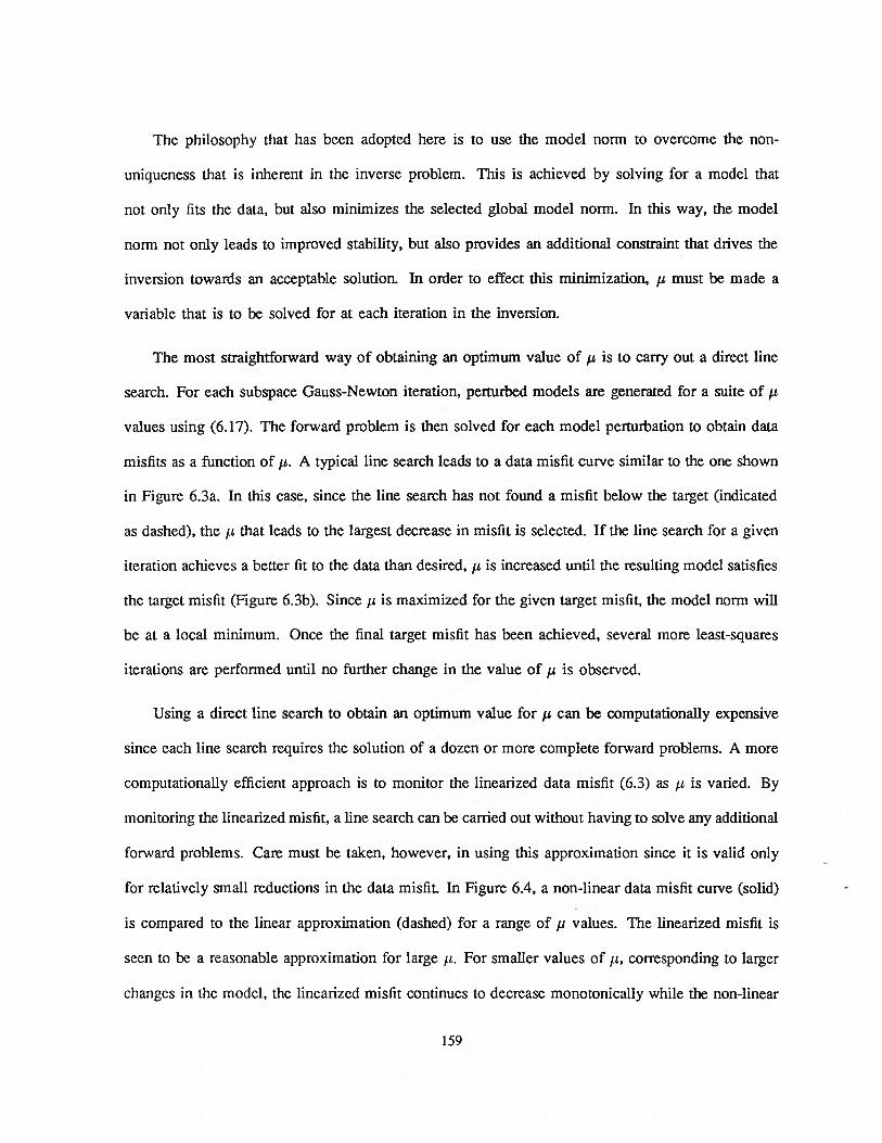
The philosophy that has been adopted here is to use the model norm to overcome the non-

uniqueness that is inherent in the inverse problem. This is achieved by solving for a model that

not only fits the data, but also minimizes the selected global model norm. In this way, the model

norm not only leads to improved stability, but also provides an additional constraint that drives the

inversion towards an acceptable solution. In order to effect this minimization, p must be made a

variable that is to be solved for at each iteration in the inversion.

The most straightforward way of obtaining an optimum value of p is to cany out a direct line

search. For each subspace Gauss-Newton iteration, perturbed models are generated for a suite of p

values using (6.17). The forward problem is then solved for each model perturbation to obtain data

misfits as a function of p. A typical line search leads to a data misfit curve similar to the one shown

in Figure 6.3a. In this case, since the line search has not found a misfit below the target (indicated

as dashed), the p that leads to the largest decrease in misfit is selected. If the line search for a given

iteration achieves a better fit to the data than desired, p is increased until the resulting model satisfies

the target misfit (Figure 6.3b). Since p is maximized for the given target misfit, the model norm will

be at a local minimum. Once the final target misfit has been achieved, several more least-squares

iterations are performed until no further change in the value of p is observed.

Using a direct line search to obtain an optimum value for p can be computationally expensive

since each line search requires the solution of a dozen or more complete forward problems. A more

computationally efficient approach is to monitor the linearized data misfit (6.3) as p is varied. By

monitoring the linearized misfit, a line search can be carried out without having to solve any additional

forward problems. Care must be taken, however, in using this approximation since it is valid only

for relatively small reductions in the data misfit. In Figure 6.4, a non-linear data misfit curve (solid)

is compared to the linear approximation (dashed) for a range of p values. The linearized misfit is

seen to be a reasonable approximation for large For smaller values of p, corresponding to larger

changes in the model, the linearized misfit continues to decrease monotonically while the non-linear

159

101 102 i0

Figure 6.3 Data misfit plotted against the ridge regression parameter p generated through the course of a non-linear line

search. a) Since the target misfit (dashed line) is not achieved, the p value corresponding to the minimum

chi-squared misfit is selected for the final perturbation. b) In this case the target misfit was achieved.

The largest p value corresponding to the target misfit is selected for the final perturbation.

25000

20000

0L0

15000

10000

101

IL

Figure 6.4 Non-linear data misfit (solid line) and linearized approximation to the data misfit (dashed

line) plotted against the ridge regression parameter p.

160

a.

misfit reaches a minimum and then increases very rapidly. Clearly the linear misfit will be a very

poor approximation in this region.

25000 25000

20000 20000

00

015000

0 ° 15000U)I I

10000C-)

10000

5000

101 102 iO

102 iO

6.3.5 Problems related to regularization

Two difficulties were encountered when regularizing the DC resistivity inverse problem. The

first arises because of the minimization of the norm of the model relative to a reference model. When

minimizing only the norm of the perturbation, the Gauss-Newton iteration is given by

= (jTj + WTW)’JT(e(rW_1)— eo6s) (6.48)

Assuming W is non-singular

lim = (WTW)_1JT(ë(ñin_1)— ëobs) = _(WTW)_1(ñi) (6.49)

Since— ( WTW)_1 (n,) is a descent direction, the Gauss-Newton iteration is guaranteed to reduce

the misfit on each successive iteration. When minimizing a norm of the model relative to a reference

model, however, the Gauss-Newton iteration is given by

ñi,= (JTJ+/T TTW) [JT(*(n_1)—

(6.50)ILWT1V(ni7

— iTiref)]

and, assuming W is non-singular

Jim = _(n_1. ñif) (6.51)

Increasing the ridge regression parameter returns the solution back to the reference model. Thus

there is no guarantee that the iteration will reduce the misfit, regardless of what ridge regression

parameter is used. Any inversion algorithm that makes use of a global model norm should therefore

be safeguarded against increases in misfit. This can be done by temporarily setting ñiref to ñ7’

and recomputing the perturbation if an increase in misfit is observed.

The second problem results from the use of a model norm only involving derivatives of the

model. Note that for the smallest energy model, where T4 = I, the matrix jTj + I must be

inverted to compute the model perturbation in (6.11). The stability of the matrix inversion results

from adding the well conditioned matrix ,til to the possibly singular matrix jTj•

161

For model norms involving only derivatives, the weighting matrix itself may not be well

conditioned. Consider, for example, the smallest Laplacian weighting matrix Wv2. The eigenvalues

of the matrix are found by solving the problem

WV2i3’=A (6.52)

For each interior node, (6.52) can be written as

v_i, + v_i — (4 + A)v, + v,,1 + = 0 (6.53)

where i = 1,.. . , M2, and j = 1,. . ., M. Using a discrete form of separation of variables (Goldberg

1986), let vjj = X1Z3. (6.53) then becomes

+ X] + + Z1]— (4+ A(k1)) = 0 (6.54)

so that for some constant 0

xi_1 + x+1 = ox(6.55)

Z_1 + Z2 = (4 + A — O)Z

The general solution to (6.53), assuming the homogeneous Dirichiet boundary conditions

= = 0(6.56)

= = 0

yields the eigenvectors and eigenvalues

(ki) . / kin ‘\ . / linjV.. =sinI Isini

\Mr+1) \.M+l

(6.57)

r.2i kin 2” hrA ‘ = 2[sln

2(M + 1)) + 2(M2 + 1)

where k = 1 ,...,M and 1 = 1, . . . , M. The condition number of l4’2 Wv2, given by

— sin2 (2(1))+2

(2(1))C/T — (6.58)

V2

(2(A1:+1)) +sin2

162

will be large. Thus there will be components of the solution that the model norm will not be very

sensitive to. From (6.57) these are seen to correspond to low frequency components of the solution.

If the data are also not sensitive to these low frequency components, then inversion of the matrix

jTj + pWWv2 will be unstable. Increasing the ridge regression parameter in an attempt to

stabilize the iteration will be largely unsuccessful.

To successfully regularize a problem it may be necessary to add a smallest model contribution

to the model objective function. For the smallest Laplacian model this yields

= IIWv2( + zm— rnref)112 + asIjñi + ñi

— ñref 112 (659)

The constant a3 controls the trade-off between smallest Laplacian and smallest model contributions

in the model objective function. Similarly, for the smallest first derivative model

= aIIW( + ini— rnref)Ij + aIIW(ni +

—

(6.60)+aIlm + Lrn

— rnrefW

6.3.6 Subspace steepest descent algorithm

Although the generalized subspace Gauss-Newton algorithm is quite efficient in terms of the

size of matrices that must be inverted, it still requires the calculation of a large number of data

sensitivities. Since forming the complete sensitivity matrix requires the solution of as many forward

problems as there are measurement locations, this can result in a rather expensive calculation. The

subspace steepest descent algorithm, an algorithm that make use of only gradient information, was

developed in an effort to address this problem.

The subspace steepest descent algorithm is a generalization of the steepest descent optimization

procedure that allows for the minimization of a global model norm. Following the procedure used

163

to develop the subspace Gauss-Newton iteration, a solution to the problem

minimize {IiW(n + Ln—

ñrej)W =

(n_1 + rn — rn ) WTW(rnfll + jrn — } (6.61)

subject to (n_1 + zñi) = (ni) + =

is sought, where the perturbation is of the form ni = G. Minimizing

O( A) = (n_1 + G& — ñtref) WTW(m?11+ Gó rnref)+

(6.62)2A((ni’) + T(ñ_1)G_ )

with respect to and A and solving for zñi yields the subspace steepest descent iteration

= n-1— G(GTWTWG)GT{WTW(ni1

— ñif) + (6.63)

where A is given by

A — —

— TG(GTWT7G)1GTWTT17(n_1— rnref)

(664)- TG(GTTTwG)’GT

Although these expressions appear complicated, they are easy to form because of the small dimension

of the matrices involved. A single iteration of the subspace steepest descent procedure involves

computing the data misfits and objective function sensitivities for the model from the previous

iteration. Since only objective function sensitivities are required in (6.63) and (6.64), the number of

forward solutions is kept to a minimum. As well, the optimum value of A can be computed without

a line search, further reducing the number of forward modeling evaluations.

Inversions that were carried out using the subspace steepest descent algorithm showed that

the linear approximation used to derive (6.63) and (6.64) was adequate for early iterations of the

inversion. For later iterations, however, the use of higher order information was needed to maintain

a good rate of convergence. A full inversion was thus carried out by using the subspace steepest

descent iteration until convergence became poor. The subspace Gauss-Newton algorithm was then

used for the remainder of the inversion. The use of this hybrid algorithm saves considerable forward

modeling evaluations, while still maintaining a good convergence rate. The use of this approach in

the solution of three-dimensional problems would be particularly advantageous.

164

6.4 Inversion of DC resistivity and MMR data

The generalized subspace approach was applied to the inversion of various DC resistivity data

sets, including data sets generated for the pole-pole, pole-dipole and dipole-dipole electrode config

urations. The use of cross-borehole pole-pole measurements to supplement surface measurements

was also examined. The objective of this work was to demonstrate the usefulness of the generalized

subspace approach in the solution of a wide variety of problems, and to examine aspects of the algo

rithm that have been discussed. The relative merits of the various data sets in resolving subsurface

structures was also of interest.

The subspace approach was also applied to the inversion of surface MMR data in an effort

to determine the usefulness of magnetic field information in resolving subsurface structures. From

comparisons of the sensitivities computed for both the MMR and DC resistivity experiments (Chapter

5) it was clear that the information contained in the two surveys is quite different. It was hoped that

the use of MMR data in a joint MMR/DC resistivity inversion might provide additional information

that might help to better resolve subsurface structures.

6.4.1 Choice of data for the inversion

In formulating a solution to a specific inverse problem it is first necessary to select an appropriate

response to use as data in the inversion. For the pole-pole potential problems, it was assumed that

the measurements ‘$obs,j , j = 1,. . . , N were contaminated with Gaussian uncorrelated errors having

a standard deviation s = ajcobs,j. The misfit function that was used to monitor the fit to the data

was the Chi-squared misfit

=

(_(i))2

(6.65)j=1 .1 obs,j

For a sufficiently large data set the expected value of the chi-squared distribution will equal the

number of data in the problem. This provides a good criterion for selecting the target misfit in an

actual inversion.

165

Data for pole-dipole and dipole-dipole inversions were taken to be the corresponding potential

differences normalized by their assumed standard deviations. Similarly, the magnetic field compo

nents normalized by their assumed standard deviations were used as data in the MMR inversions.

6.4.2 Development of the 2D inversion algorithm

Having decided on a suitable choice for the data, errors, and misfit criterion, an inversion

algorithm based on the generalized subspace approach was developed to invert various DC resistivity

and MMR data sets. To compute the predicted data required in the inversion, the 2D finite difference

program described in Chapter 2 was used. The code is accurate for a wide range of problems, and

is quite flexible in terms of the kinds of models and survey geometries that can be accommodated.

It is also quite efficient, particularly if the problem must be solved for many different right hand

sides. The sensitivities for the DC resistivity and MMR responses were also computed using the

finite difference code, making use of the adjoint equation formulation developed in Chapter 5.

In defining a basis set for the subspace approach, separate data misfit sub-objective functions

were associated with each current electrode or current dipole in the survey. The steepest descent

directions associated with each sub-objective function were then used to form the basis set. The

algorithm also allowed for the possibility of further subdividing the data set into near and far offset

data, down well and cross-well data, and other groupings. For problems where joint inversions were

to be carried out, separate sub-objective functions were defined for each of the different responses.

In addition to the basis vectors derived from the data misfits, the algorithm also allowed for the

use of other basis vectors to accelerate convergence and facilitate minimization of the model norm.

These include the steepest descent direction of the global model norm, linear functions of depth and

other linear trends, layers, rectangular cells, high and low frequency components of the solution, and

perturbations from previous iterations.

166

Regularization of the inversion was effected by minimizing a global model norm at each iteration

of the inversion. The algorithm allowed for the use of various weighting matrices to define the

appropriate model norm. In most cases the norm corresponding to the weighted sum of the energy in

the first derivatives of the model (6.36) was used. This particular norm has considerable flexibility

since it allows for a trade-off between smoothness in each of the two directions. The reference model

that was used in most cases was a uniform halfspace, although an arbitrary conductivity structure

could be specified.

To obtain a minimum in the model norm at each iteration, a line search making use of either the

linear or non-linear data misfit was used to determine the appropriate value for the ridge regression

parameter. In most cases the line search based on the linear approximation was only useful for the

first few iterations. For later iterations, it was usually necessary to switch to a line search based on

the non-linear misfit to further improve the fit to the data. At each iteration, the line search attempted

to reduce the data misfit by 50% until the target fell below the expected chi-squared misfit, at which

point the target was set to the expected misfit. Once the inversion had achieved the expected chi

squared misfit, further iterations were carried out in an effort to further reduce the global model norm.

The inversion was terminated after a fixed number of iterations, or once changes in the solution were

no longer observed.

The resulting algorithm was quite flexible in terms of the models that could be recovered and the

types of data that could be inverted. Data for almost any electrode configuration for either the MMR

or DC resistivity problem can be used in the inversion. Source and measurement locations can be

located on the surface or placed at depth to simulate a cross-borehole configuration. A fixed regional

conductivity structure can be specified, or it can be left as an unknown in the inversion. Topography

can also be represented in the problem. Extensive testing of the algorithm was carried out for various

models and synthetic data sets. The results of this testing were, on the whole, quite successful and

demonstrated the power of the generalized subspace approach. Applications of the algorithm to the

167

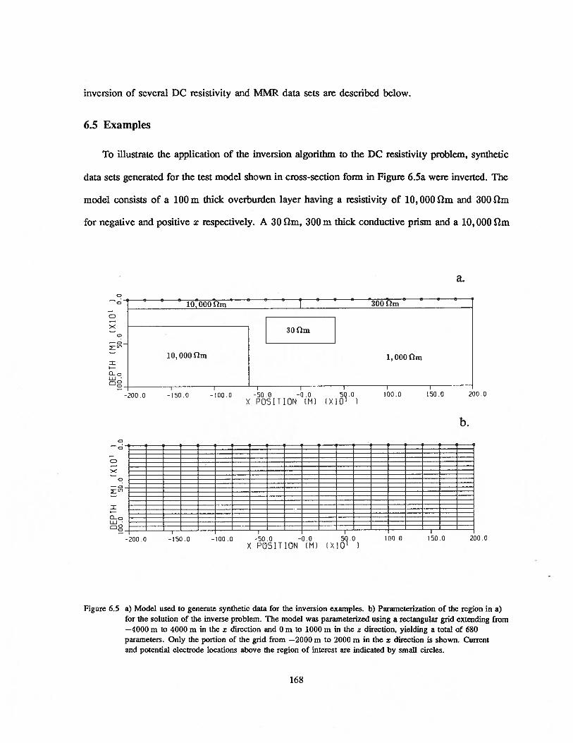
inversion of several DC resistivity and MMR data sets are described below.

6.5 Examples

To illustrate the application of the inversion algorithm to the DC resistivity problem, synthetic

data sets generated for the test model shown in cross-section form in Figure 6.5a were inverted. The

model consists of a 100 m thick overburden layer having a resistivity of 10,000 m and 300 1m

for negative and positive x respectively. A 30 Qm, 300 in thick conductive prism and a 10,000 m

a.0

e S e ‘ - , e a a S — a S p p

0 10 000 fm 300 Zm

30m

10,000fm 1,O00fm

0LUo

_______________________ ____________________________________________

0_I I I I

-200.0 —150.0 —100.0 —50.0 —0.0 5Q.0 100.0 150.0 200.0X POSITION (M) IXIO’

b.0

>< ——

0 — — — — — — — — — —

—C- — — — — — — — — — —

— — — — — — — — — —

El EE El. El El El El El El El El El El

0-c, — — — — — — — — — — — — — — — — — — — —uJ. —

00

-200.0 -150.0 -100.0 -50 0 —0.0 5Q.0 100 0 150.0 200.0X POSITION (M) (XIO’ I

Figure 6.5 a) Model used to generate synthetic data for the inversion examples. b) Parameterization of the region in a)for the solution of the inverse problem. The model was parameterized using a rectangular grid extending from—4000 m to 4000 m in the x direction and 0 m to 1000 m in the z direction, yielding a total of 680parameters. Only the portion of the grid from —2000 in to 2000 in in the z direction is shown. Currentand potential electrode locations above the region of interest are indicated by small circles.

168

resistive ledge are buried below the layer in a 1,000 fm uniform background. The model was

parameterized using a rectangular grid extending from —4000 m to 4000 m in the x direction and

0 m to 1000 m in the z direction, yielding a total of 680 parameters. The region of interest, in this

case the portion of the grid from —2000 m to 2000 m in the x direction, is shown in Figure 6.5b

and subsequent cross-sections.

To image the region of interest, 21 current electrodes were placed along the surface every 200 m

from —2000 m to 2000 m. On either side of each current electrode, 5 potential electrodes were placed

200 m apart, yielding a total of 10 pole-pole potential readings for each current gather. The integrated

finite difference algorithm described in Chapter 2 was then used to model the 210 pole-pole potentials

to be used in the first set of inversions.

6.5.1 Inversion of pole-pole responses

For the first set of examples, 5% Gaussian noise was added to the modeled pole-pole potentials,

and the data were then inverted using the generalized subspace algorithm. A 500 lm uniform

halfspace was used as both the starting model and reference model. Note that this is not the same as

the true background resistivity of 1000 !m. A total of 22 basis vectors (one corresponding to each

current electrode sub-data misfit function and an additional one corresponding to the global model

norm) were used to form the subspace in this set of examples. To regularize the inversion, the model

objective function given in (6.60) was minimized. Values of (a3,a, a) = (1 x iO, 10,1) were

selected for the coefficients controlling the trade-off between energy and energy in the derivatives in

the x and z directions. This choice of coefficients was based on experimentation, and was found to

be suitable for a wide variety of models and survey geometries. The results of the inversion after

3, 5, 15 and 40 iterations are shown in cross-section form in Figure 6.6. Because of the difficulty

in generating adequate greyscale displays for comparing the different results, contour displays were

169

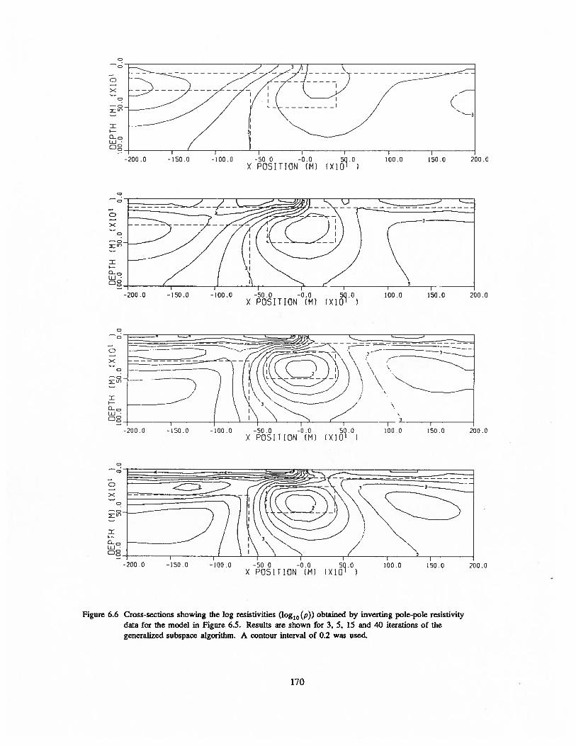
-r1

—,, 0

(o

8 C o.-

‘1

0 c

C

0

0

used. The inversion was successful in recovering all features in the true model. Both the conductive

and resistive sections of the surface layer and the resistive bench were well resolved. The buried

conductive prism was also recovered, although its boundaries are somewhat less certain. To examine

the convergence of the inversion algorithm, the model nonn and chi-squared misfit are shown for each

iteration in Figure 6.7. The algorithm is seen to have converged quickly for the firstS iterations, after

which a somewhat poorer rate of convergence was observed. This is due to the difficulty in removing

the conductive surface layer that has appeared on the left of the model in Figure 6.6b. In spite of

this problem, the algorithm was able to achieve a solution that fit the data to the target chi-squared

misfit after 25 iterations. No further change in the solution was observed for subsequent iterations.

The use of the linearized misfit to carry out the line search for the first 8 iterations yielded essentially

the same results as shown in Figure 6.6, although the cost of the inversion was about 15% less.

i°4

Cl,

E

C)

0DCCl,

(-I

10 20 30 10 20 30

Iteration number Iteration number

Figure 6 7 Convergence of the generalized subspace algorithm for the results in Figure 6 6 a) Chi squared misfit for eachiteration The target misfit of 210 is indicated by the dashed line b) Global model norm for each iteration

To illustrate how the convergence rate of the solution can be influenced by the choice of basis

vectors, the same inversion was carried out using the two basis vector formulation proposed initially

by Kennett and Williamson (1987). In this formulation only the steepest descent directions of the

data misfit and global model norm objective functions are used in the inversion. The result after 40

171

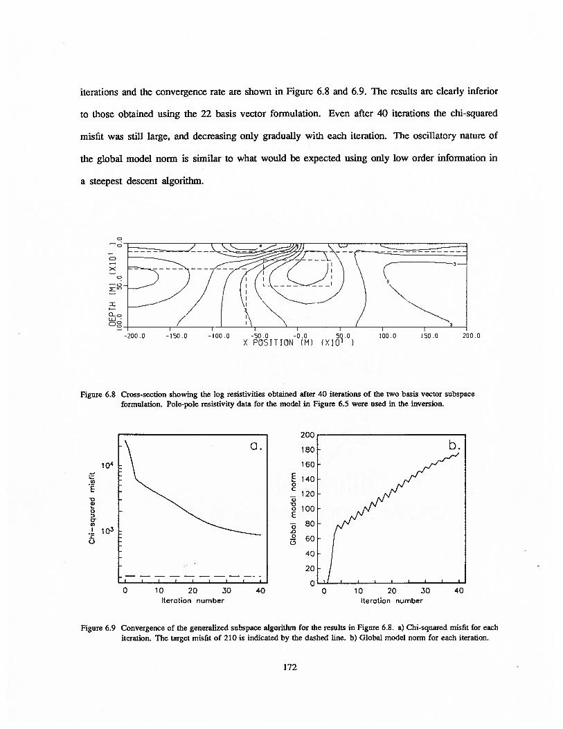
Figure 6.8 Cross-section showing the log resistivities obtained after 40 iterations of the two basis vector subspaceformulation. Pole-pole resistivity data for the model in Figure 6.5 were used in the inversion.

Figure 6.9 Convergence of the generalized subspace algorithm for the results in Figure 6.8. a) Chi-squared misfit for eachiteration. The target misfit of 210 is indicated by the dashed line. b) Global model norm for each iteration.

iterations and the convergence rate are shown in Figure 6.8 and 6.9. The results are clearly inferior

to those obtained using the 22 basis vector fonnulation. Even after 40 iterations the chi-squared

misfit was still large, and decreasing only gradually with each iteration. The oscillatory nature of

the global model nomi is similar to what would be expected using only low order information in

a steepest descent algorithm.

0

JO 0-50 0 -0.0 5Q.OX POSITION (Ml (XlO’

a.i04

C,)

E•0

0

0U)

iOC-)

E0C

a)-o0

E

0

0(7

0I I I

10 20 30Iteration number

40 0 10 20 30 40

Iteration number

172

C

><

—c

_____ _____

i: Lfl

____ ____ ____ ____ ____ ____ ____

-

____

CuJ.— I

200(1 —150.0 -100.0 —50.0 —0.0 5Q.0 101.0 150.0X POSITION (Ni) {XlO’

Since reducing the dimension of the subspace leads to poorer result, adding additional vectors

to the original basis set should lead to an improvement. To show that this is the case, an inversion

was carried out using the 22 basis vector set and an additional set of 95 “blocky” basis vectors. The

new basis vectors were generated by subdividing the model into a set of 95 rectangular cells, with

cells being made finer in region below the electrodes. The subdivisions used to generate the basis

vectors are shown for the region of interest in Figure 6.lOa.

a.9

200 (1

.0

0

b.

Figure 6.10 Results of the generalized subspace inversion of pole-pole data using additional “blocky” basisvectors, a) Cross-section showing the sub-regions used to define the “blocky” basis vectors inthe region of interest. b) Cross-section showing the log resistivities obtained after 40 iterationsPole-pole resistivity data for the model in Figure 6.5 were used in the inversion.

173

Each additional basis vector was taken to be unity over one of the cells and zero elsewhere. The

result of this inversion after 40 iterations and the convergence rate are shown in Figure 6. lOb and

Figure 6.11. As seen in Figure 6.11, the use of the additional basis vectors increases the convergence

rate of the algorithm considerably, although each iteration requires about 3 times as much execution

time as a 22 basis vector iteration. The use of this larger basis set does not significantly improve

the final solution, as can be seen by comparing Figure 6.6d to Figure 6.lOb. It does, however,

demonstrate that the final inversion result has not been degraded by the use of only 22 basis vectors

in the original formulation.

The convergence rate of the inversion clearly depends on the choice of basis vectors used in the

subspace formulation. As well, the convergence rate will also depend on the degree of smoothness

that is imposed on the solution by the choice of model norm. To illustrate this, inversions were carried

out for the 22 basis vector problem using both larger and smaller values of ct9, the parameter that

controls the relative contribution of the smallest energy component in the global model norm. The

inversion results after 40 iterations are shown in Figure 6.12, and the data misfits and global model

norms for each iteration are shown in Figure 6.13. In both cases, the inversion has not yet converged

a.

I I

1 4

E.2E C

00 -o

0

E0 —

0) aiO

- .2(.) 0

0 10 20 30 40 0 10 20 30 40Iteration number Iteration number

Figure 6.11 Convergence of the generalized subspace algorithm for the results in Figure 6.10. a) Chi-squared misfit foreach iteration. The target misfit of 210 is indicated by the dashed line. b) Global model norm for each iteration.

174

to a model that fits the data. For the choice of the larger value of a, the inversion is permitted to

build up excessive amounts of structure near the surface that is not easily removed at later iterations.

For the smaller value of a3, the basis vectors become excessively smooth, and cannot duplicate the

rapid changes in resistivity that are needed to satisfy the data. The oscillatory nature of the global

model norm (Figure 6.13c) for this result is typical of an inversion that is too strongly regularized.

The descent vectors that are used to construct the perturbation at each iteration become almost parallel

to the level lines of the misfit objective function, leading to an oscillation between two different points

a.

Figure 6.12 Cross-sections showing the log resistivities obtained by inverting pole-pole resistivity data for the model in

Figure 6.5. a) Result obtained using c. I x iO. b) Result obtained using . = 1 x 1O.

b.

—50 0 -0.0 50.0X POSITION (M) rxiO

175

in model space. These oscillations can be reduced and faster convergence achieved by supplementing

the basis set with vectors corresponding to perturbations from the previous two iterations. The result

obtained after 40 iterations, shown in Figure 6.14, was a considerable improvement over that obtained

without the two additional vectors (Figure 6. 12b). In particular, the region on the left side of the

model is much better resolved. The overall convergence rate, shown in Figure 6.15, is also improved.

E

0D0U,

.1C-)

E•0

0D0

-cC)

Figure 6.13 Convergence of the generalized subspace algorithm for two choices of a. a) Chi-squared misfit for

each iteration for a — 1 x i0. The target misfit of 210 is indicated by the dashed line. b) Global

model norm for each iteration for a — 1 x i04. c) Chi-squared misfit for each iteration for

o = 1 x 10. d) Global model norm for each iteration for a = I x l0.

iO

a.

E0C

Q)

0E

C.00

0 10 20 30 40Iteration number

1 o

Iteration number

C.250

200

150

100

50

E0C

0-o0

EC-o0

C-)

0 10 20 30iteration number

400

0 10 20 30iteration number

40

176

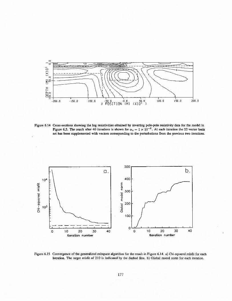
.0

Figure 6.14 Cross-sections showing the log resistivities obtained by inverting pole-pole resistivity data for the model inFigure 6.5. The result after 40 iterations is shown for s = 1 x 10_B. At each iteration the 22 vector basisset has been supplemented with vectors corresponding to the pertorbations from the previous two iterations.

40

Figure 6.15 Convergence of the generalized subspace algorithm for the result in Figure 6.14. a) Chi-squared misfit for eachiteration. The target misfit of 210 is indicated by the dashed line. b) Global model norm for each iteration.

177

-500 -0.0 50 0X POSITION (MI (X1O’ I

0.

(Il

E0

0

U,

-cC-)

i0

0

B)-o0E

0-o0

C-)

I i Li —— 1 --

0 10 20 30Iteration number

40 0 10 20 30Iteration number

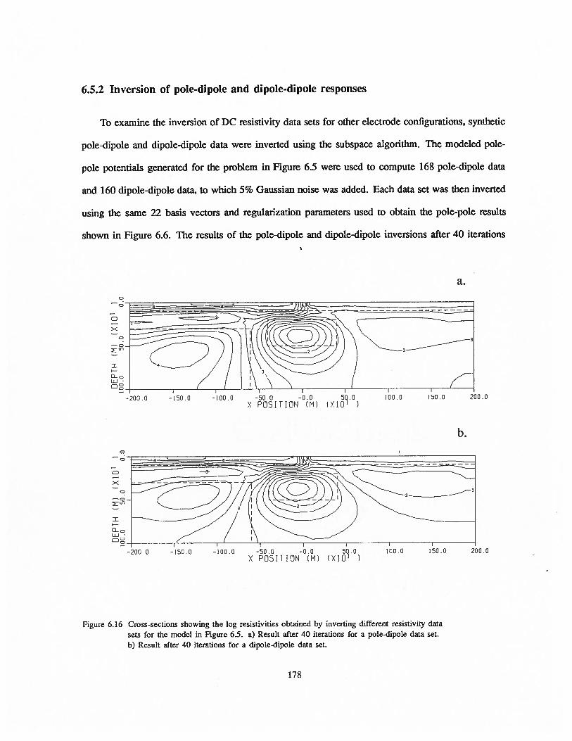
6.5.2 Inversion of pole-dipole and dipole-dipole responses

To examine the inversion of DC resistivity data sets for other electrode configurations, synthetic

pole-dipole and dipole-dipole data were inverted using the subspace algorithm. The modeled pole-

pole potentials generated for the problem in Figure 6.5 were used to compute 168 pole-dipole data

and 160 dipole-dipole data, to which 5% Gaussian noise was added. Each data set was then inverted

using the same 22 basis vectors and regularization parameters used to obtain the pole-pole results

shown in Figure 6.6. The results of the pole-dipole and dipole-dipole inversions after 40 iterations

0

><

0

0

0LU

Figure 6.16 Cross-sections showing the log resistivities obtained by inverting different resistivity datasets for the model in Figure 6.5. a) Result after 40 iterations for a pole-dipole data set.b) Result after 40 iterations for a dipole-dipole data set.

a.

.0

200.0

b.

-200.0 —0.0 —100.0 —50 0 —0.0 50.0 100.0 150.0X POSITION (Mi (XlO’ I

178

are shown in Figure 6.16. In both cases the target chi-squared misfit was achieved, although the

convergence was slower than in the pole-pole case. The final results are quite similar to the pole-pole

result, (Figure 6.6d), although somewhat better resolution appears to have been achieved using the

pole-dipole and dipole-dipole data sets.

6.5.3 Inversion of cross-borehole pole-pole responses

A further investigation was carried out to examine the use of cross-borehole data to further

constrain the inversion of surface pole-pole data. For the purposes of the cross-borehole examples

the model used in the previous examples was retained. The location of the borehole and surface

electrode positions is shown in Figure 6.17a. Because of the denser data set that was to be inverted,

the model was parameterized using a finer discretization over a smaller region than in the previous

examples. In this case a rectangular grid extending from —2000 rn to 2000 m in the x direction and

0 m to 2000 m in the z direction was used, yielding a total of 1024 parameters. The portion of the

grid from —l000m to l000m in the x direction and Urn to l000rn in the z direction is shown in

Figure 6.17b and subsequent cross-sections.

To image the region of interest, 5 electrodes were placed every 200 m in each of the two wells.

An additional 11 electrodes were placed on the surface every 200 m from —1000 m to 1000 m. For

current injected at a particular electrode, potentials at each of the remaining electrodes were modeled,

resulting in a total of 420 synthetic pole-pole data. 5% Gaussian noise was again added to the modeled

pole-pole potentials, and the data were inverted using the generalized subspace algorithm. In this

inversion, three basis vectors were associated with each current electrode gather — one corresponding

to potential electrodes in each of the two wells, and one corresponding to surface potential electrodes.

All other parameters for the inversion were identical to those used to obtain the pole-pole results

shown in Figure 6.6. The result after 40 iterations is shown in Figure 6.18. Resolution of all features

of the model was found to be excellent. The resistivilics of the various features were very close

179

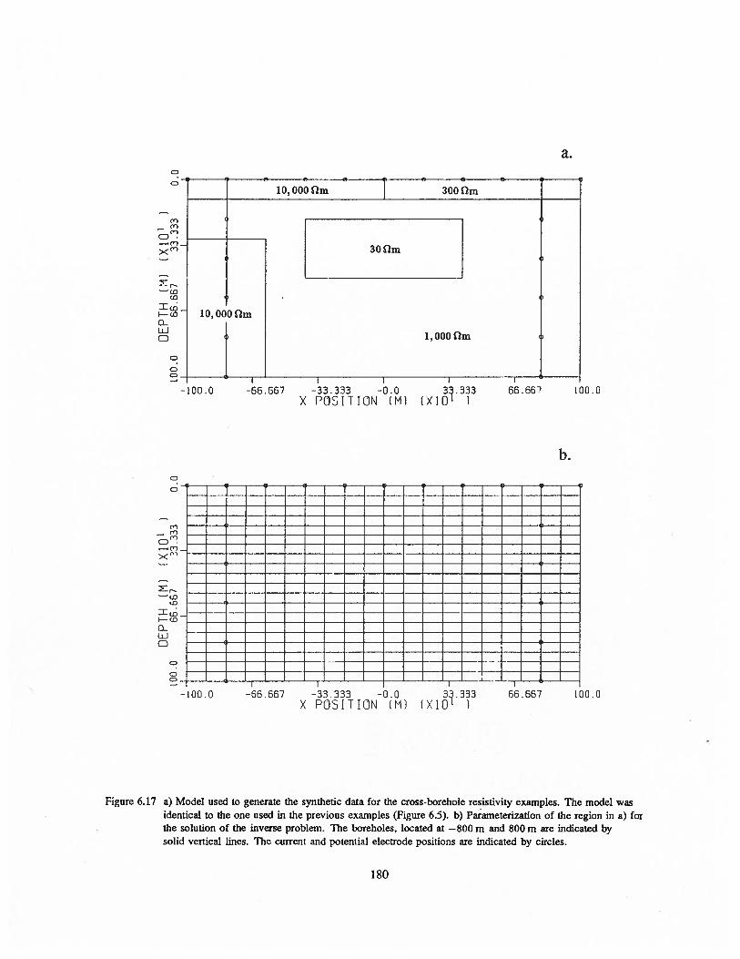
a.

CD

I.- CD

abJ0

C,-)— C,-)

— Cr) -

>< en

CDCo

lCd.I— CO

aUi0

0

b.

Cr)-

— Cr)

>< C)

-

—100.0 -56.567 -33333 -.0 3.333 66.667 100.0X POSITION IM) (X1O’ 1

Figure 6.17 a) Model used to generate the synthetic data for the cross-borehole resistivity examples. The model wasidentical to the one used in the previous examples (Figure 6.5). b) Parameterization of the region in a) forthe solution of the inverse problem. The boreholes, located at —800 m and 800 m are indicated bysolid vertical lines. The current and potential electrode positions are indicated by circles.

180

to their true values, and the boundaries of the buried conductor were extremely well defined. The

convergence rate observed for this inversion, shown in Figure 6.19, was also excellent. The inversion

was able to achieve the target misfit of 420 after only 12 iterations.

—100.0 —66.667 —33.333 —0.0 3.333 100.0X POSITION (M) (X1O’

Figure 6.18 Cross-section showing the log resistivities obtained by inverting cross-borehole pole-pole resistivitydata for the model in Figure 6.17. The result after 40 iterations is shown.

Co- Co

cD— Co

><.,

— (C(0

H-CD

0LU0

C

66.C7

181

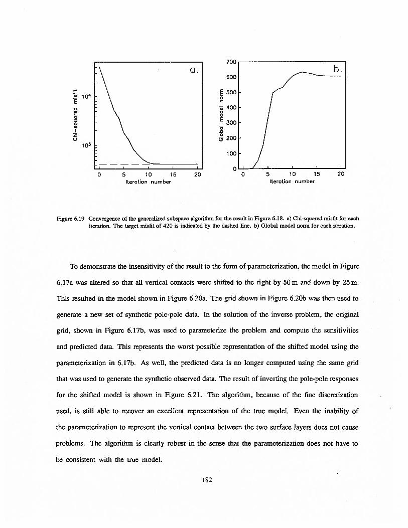
700

600

E500. i0E c

400

E300U)

o C,1 o

100

010 15

Iteration number

Figure 6.19 Convergence of the generalized subspace algorithm for the result in Figure 6.18. a) Chi-squared misfit for eachiteration. The target misfit of 420 is indicated by the dashed line. b) Global model norm for each iteration.

To demonstrate the insensitivity of the result to the form of parameterization, the model in Figure

6. 17a was altered so that all vertical contacts were shifted to the right by 50 m and down by 25 m.

This resulted in the model shown in Figure 6.20a. The grid shown in Figure 6.20b was then used to

generate a new set of synthetic pole-pole data. In the solution of the inverse problem, the original

grid, shown in Figure 6. 17b, was used to parameterize the problem and compute the sensitivities

and predicted data. This represents the worst possible representation of the shifted model using the

parameterization in 6. l7b. As well, the predicted data is no longer computed using the same grid

that was used to generate the synthetic observed data. The result of inverting the pole-pole responses

for the shifted model is shown in Figure 6.21. The algorithm, because of the fine discretization

used, is still able to recover an excellent representation of the true model. Even the inability of

the parameterization to represent the vertical contact between the two surface layers does not cause

problems. The algorithm is clearly robust in the sense that the parameterization does not have to

be consistent with the true model.

a.

0 5 20 0 5 10 15 20Iteration number

182

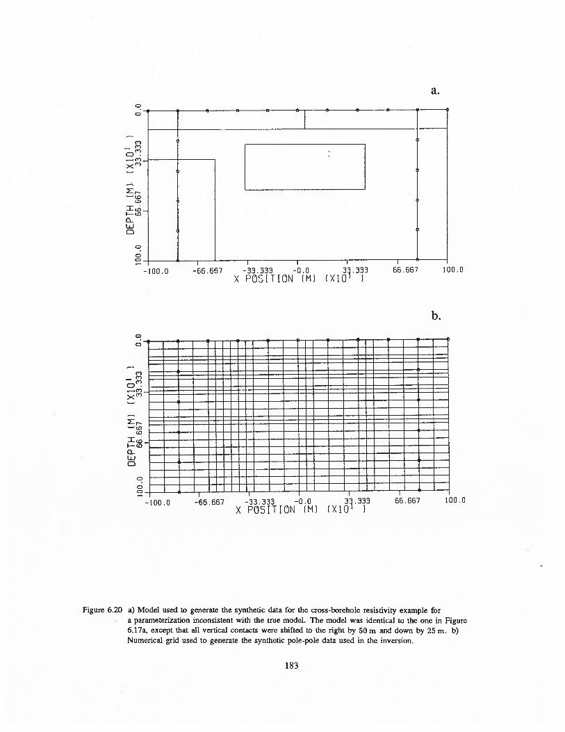
‘1

zp

8

cc

‘

><

,t3

)

(-nh)

gC)

C)

cJJ

—.

C)

><

0

U)

C)

U)

CD

01- 0

0

DEP

TH(M

).(X

10

1I

100.

06

66

67

33.3

33

0.0

cD a, 0)

0)

><

U)

U)

U)

U)

U)

U)

0)

0) a, 0)

pp

—

100.0

Figure 6.21 Cross-section showing the log resistivities obtained by inverting cross-borehole pole-pole resistivitydata for a shifted version of the model in Figure 6.17. The result after 40 iterations is shown. Theparameterization used in the solution of the inverse problem is shown in Figure 6.17b.

To illustrate the importance of borehole data, an inversion using only the surface data for the

problem in Figure 6.17 was attempted. The result after 40 iterations is shown in Figure 6.22. The

ability of this particular data set to image the subsurface is clearly quite poor. The image of the

buried conductor is extremely diffuse, and its center has been shifted to the left by about 100 m. The

presence of the resistive ledge is also not detected.

(9—(9

—(9.>< (9

CDCD

CDCu-i0

—100.0 -66.667 -33.333 -0.0 3.333 66.667X POSITION (M) (X1O1

184

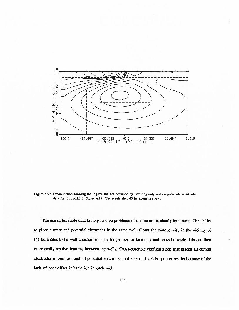
100 0

Figure 6.22 Cross-section showing the log resistivities obtained by inverting only surface pole-pole resistivitydata for the model in Figure 6.17. The result after 40 iterations is shown.

The use of borehole data to help resolve problems of this nature is clearly important. The ability

to place current and potential electrodes in the same well allows the conductivity in the vicinity of

the boreholes to be well constrained The long-offset surface data and cross-borehole data can then

more easily resolve features between the wells. Cross-borehole configurations that placed all current

electrodes in one well and all potential electrodes in the second yielded poorer results because of the

lack of near-offset information in each well.

C,-)— ()

— C’_)

CDCD

I— CD

0uJ0

-33.333 -0.0 3.333)< PO5IIION (Mi IXIU’ I

185

6.5.4 Inversion of MMR responses

To assess the ability of magnetic field information to resolve the subsurface, MMR data sets

were inverted using the generalized subspace algorithm. Synthetic B, B and B magnetic field

components for the problem in Figure 6.5 were computed for each station used in the first pole-pole

example. The stations in this case were offset 500 m in the y direction from the current electrodes.

As before, 5% Gaussian noise was added to the modeled data. Each data set was then inverted

separately using the same 22 basis vectors and regularization parameters used to obtain the pole-pole

results shown in Figure 6.6. The results of the MMR inversions after 20 iterations are shown in

Figure 6.23 and the respective convergence rates are shown in Figure 6.24.

Inversions using the B and B data sets fit the target misfit after 12 iterations and yielded

similar results. In both cases the top of the buried conductor and the conductive section of the layer

on the right were well resolved, although the resistive features on the left were undetected. The

recovered resistivities were also biased towards lower resistivities. This is not surprising considering

the MMR responses are sensitive only to the relative resistivity — absolute values of resistivity cannot

be obtained using only magnetic field information. Because of this, the inversion algorithm is free

to add a constant to the resistivity model without changing the misfit to the observed data.

The inversion of the B data set was also able to resolve the buried conductive target. Although

the inversion was unable to fit the data after 20 iterations, the conductive structure was still visible

in the recovered model. An examination of the sensitivities for the B component suggested that

this component is more sensitive to near surface vanations in the conductivity This high sensitivity

may have resulted in the slow convergence observed for this irn ersion To obtain a better rate of

convergence, it may be necessary to augment the standard basis set, or to make use of a different

regularization scheme.

186

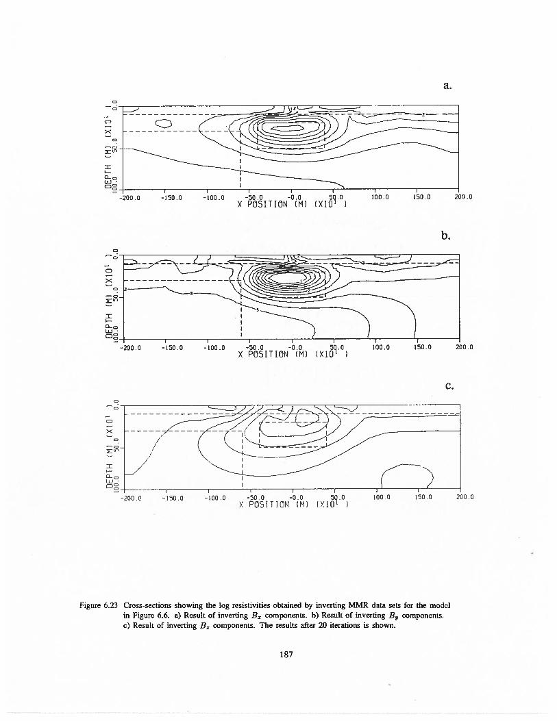
.-11

1 CD t.)

pg.

CD 8

.CD

D -.

C)CD

—‘

CD

,-1

co ..—

— ni. “

C CD ‘-0

OEP

TH(M

)(X

1fJ

100.0

50

.0

>< -tJ

QD

Cf)

o

0

0•

b

02

C

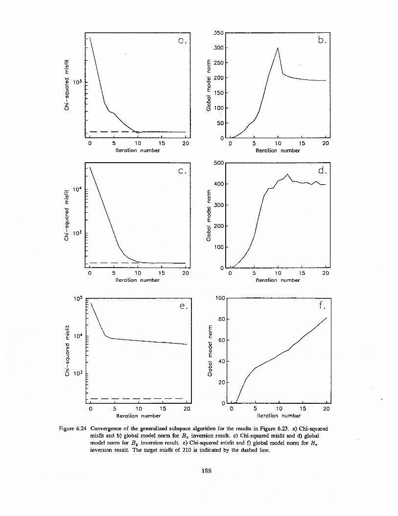
0,

E

0 5 10 15 20terotion number

E

E - C

-v -a,0

D E0(a -

I -

o

0 5 10 15 20terotion number

io5

E4 0

E 10 c

-

a, -o0

DC

.0

C) C,

0 5 10 15 20iteration number

Figure 6.24 Convergence of the generalized subspace aigorithm for the results in Figure 6.23. a) Chi-squaredmisfit and b) global model norm for B,, inversion result. c) Chi-squared misfit and d) globalmodel norm for B inversion result. e) Chi-squared misfit and f) global model norm for B,inversion result. The target misfit of 210 is indicated by the dashed line.

188

a.

E0C

a,-C0

E

0.00

(3

C.

iteration number

Iteration number

e.

0 5 10 15 20iteration number

6.5.5 Joint inversion of MMR and pole-pole resistivity responses

The inversion of various synthetic MMR data sets was generally found to be successful in

recovering highly resolved images of conductive targets. The use of magnetic field information

alone, however, was unable to completely resolve other features of the model. In particular, resistive

targets and ‘ayered structures were often poorly resolved, and only relative resistivities could be

obtained from the data. In contrast, the use of only potential field information generally led to a

more complete image of the subsurface, although resolution was often poor. It was hoped that a joint

a.

0

Figure 6.25 Cross-section showing the log resistivities obtained by inverting pole—pole potentiai and

B MMR data sets for the model in Figure 6.6. a) The result of jointly inverting the two

data sets. b) The result of inverting only the pole-pole potential data.

189

b.

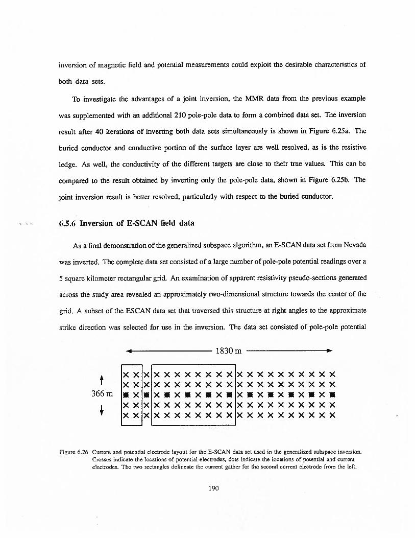
inversion of magnetic field and potential measurements could exploit the desirable characteristics of

both data sets.

To investigate the advantages of a joint inversion, the MMR data from the previous example

was supplemented with an additional 210 pole-pole data to form a combined data set. The inversion

result after 40 iterations of inverting both data sets simultaneously is shown in Figure 6.25a. The

buried conductor and conductive portion of the surface layer are well resolved, as is the resistive

ledge. As well, the conductivity of the different targets are close to their true values. This can be

compared to the result obtained by inverting only the pole-pole data, shown in Figure 6.25b. The

joint inversion result is better resolved, particularly with respect to the buried conductor.

6.5.6 Inversion of E-SCAN field data

As a final demonstration of the generalized subspace algorithm, an E-SCAN data set from Nevada

was inverted. The complete data set consisted of a large number of pole-pole potential readings over a

5 square kilometer rectangular grid. An examination of apparent resistivity pseudo-sections generated

across the study area revealed an approximately two-dimensional structure towards the center of the

grid. A subset of the ESCAN data set that traversed this structure at right angles to the approximate

strike direction was selected for use in the inversion. The data set consisted of pole-pole potential

1830m

A XX XXXXXXXXXXT xx xxxxxxxxxx

366m. x•xxxx

I xxxxxxxxxxy

Figure 6.26 Current and potential electrode layout for the E-SCAN data set used in the generalized subspace inversion.

Crosses indicate the locations of potential electrodes, dots indicate the locations of potential and currentelectrodes. The two rectangles delineate the current gather for the second current electrode from the left.

XxXXxxxxxxxxXxxxxxxsxxsx•

xxxXxXxxxxxxxxxXxx

190

- CD

CD

0-i

CD

go

)—0

—C

D•

II0

oo

—CD

HCD CD

Hg

.0

CD

Dep

th(m

)

C)

Z\D

cD

00

00

oo

0o

o

III’

IIiI

IIJII

IIII

III.

1 _

CDCD

CDfl)

C,,

dSD

<CD

CD -lC

DC

DC

CDCD

-—

CD—

.CD

,-

C,

I—’

• -laC

CD

CD

c,.,•

Ep’

CD

C,,

CDCD

D

e—

aCD

2CD

CD

CDCD

——

i-

CD

gCD

CD -CD C

,,

;D

CD

p.’-

ci

CD-

CDD)

CDg

CD- C

‘

CD-

0CD

--

CD-

0’

CDCD

00

-

CD0

CDCD

CD-

-iCD

0•

CDCD

I—

CDCD

CD-

—

CDCD

-CD

CDCD

C,D

CD C,,

CD

_

CDCD

‘C

CDCD

‘CCD

CCD

ga

CD-

CD—

C’,

00

I—

0001—

009—

009—

00-f

r—>< -

00

—C —

.0

0

00

00f

00

9

00

9

0001

001

,—

0rj

C—

.CD CD -<

-‘

0CD

—.

C,,

C/) CD

CD ‘‘

CDCD

Q -0

‘Ca

aC

-i

CD

CDC

CD-

CD-

oCD

-lo CD

)CD ‘C

CD-

0C.

’)CD

CD>

CDCD

C..’)

•

a‘,

CD CDCD

cCD

-CD

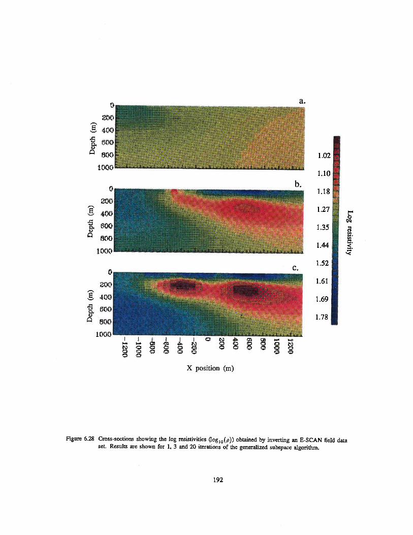
04f1A)i

4cx

600

I

C.

1.02

1.10

l.18

1.27

1.35

1.44

1.52

1.61

1.69

1.78

X position (m)

Figure 6.28 Cross-sections showing the log resistivities (1og10(p)) obtained by inverting an E-SCAN field dataset. Results are shown for 1, 3 and 20 iterations of the generalized subspace algorithm.

I 4.. 0’.i. a a a a

t . C C C C Ca a a a aa a

192

at most 2 percent for the modeled potentials. The grid was then used to define the parameterization

for the inverse problem, yielding a total of 900 parameters.

In formulating the generalized subspace inversion, a basis vector corresponding to the steepest

descent directions for the data misfits associated with each current electrode gather was defined.

An additional basis vector corresponding to the steepest descent direction for the global model

objective function was also defined. This yielded 11 basis vectors in total. The parameters defining

the weighting matrix used to regularize the problem were identical to those used in the synthetic

examples. The results of the inversion, shown after 1, 3 and 20 iterations are shown in Figure 6.28.

The convergence rate, and the apparent resistivity pseudo-section generated for the observed and

predicted data for the final iteration are shown in Figures 6.29 and 6.30 respectively. The inversion

converged quickly, achieving the target misfit in only 9 iterations. The recovered model indicates

a pair of well resolved conductors centered at (x, z) = (—400,200) m and (x, z) (600, 200) m.

Above the conductive region is a variable, highly resistive near surface layer. A deep, resistive

region to the left of the section is also visible.

50

40E

E— 30

-o a

0D

-200

-o

(_)

10

0

0 5 10 15 20 0 5 10 15

teration number Iteration number

Figure 6.29 Convergence of the generalized subspace algorithm for the results in Figure 6.28. a) Chi-squared misfit for

each iteration. The target misfit of 680 is indicated by the dashed line. b) Global model norm for each iteration.

a. b.

20

193

a.

1.24

1.27

1.31

1.340

1.37

1.40

1.44

1.47

1.50

1.53

Figure 6.30 Comparison of a) the observed apparent resistivities and b) the apparent resistivities predicted by the final

inversion result. The predicted apparent resistivities are shown for the inversion result after 20 iterations.

b.

X position (m)

194

Although there were several wells in the area, much of the geological information was con

fidential, and hence not available for confirming the results of the inversion. The company that

had aquired the data did, however, provide several highly schematic geological cross-sections which

indicated the presence of intermittent silicified clays overlying a more resistive andesite basement.

The depth of these silicified clays, and their potentially high conductivity, was consistent with the

anomalies that were recovered in the inversion. To further investigate the nature of these anoma

lies, more detailed geological information and information about the electrical conductivities of the

various units would be required.

6.6 Conclusions

Because of the problems that have been encountered in the past, a new strategy for the parametric

inversion of DC resistivity data was needed. In an effort to make the solution of the inverse problem

less dependent on the choice of parameterization, a large number of parameters were used in the

formulation. The use of a generalized subspace approach was developed to make the solution of

these large-scale problems practical.

For a suitable choice of basis vectors the convergence rate of the generalized subspace algorithm

was found to be good to excellent. Using more basis vectors in the formulation was found to improve

the rate of convergence, but also increased the cost of the inversion. A good compromise was to define

data misfit objective functions for each current electrode and to use the corresponding steepest descent

directions as basis vectors. An additional vector corresponding to the steepest descent direction of the

global model norm was also included. Convergence of the algorithm using this expanded basis set

was found to be considerably superior to that obtained using only the original two-vector formulation.

Convergence was also found to be influenced by the choice of global model norm used to control

the smoothness of the solution. For norms that did not emphasize smoothness, the solution often

displayed excessive structure, and sometimes became trapped in a local minimum. The use of a

195

model norm that excessively emphasized smoothness, however, could also lead to slow convergence

in some cases.

The use of linearized information to carry out line searches for early iterations was examined,

and found to be useful in reducing the number of forward modeling evaluations. The need to use

higher order information to achieve a good rate of convergence for later iterations was recognized. A

subspace approach based on the steepest descent algorithm was also examined. This approach also

avoided a large number of forward modeling evaluations and the inversion of large matrices.

The inversion of synthetic DC resistivity data sets for various electrode configurations and models

was used to illustrate the versatility of the generalized subspace algorithm. The inversion of pole-

pole, pole-dipole and dipole-dipole data were found to yield similar results, although the resolution

of the pole-dipole and dipole-dipole data was generally better. The use of cross-borehole data to

supplement surface data in an inversion was found to be particularly successful in obtaining a high

resolution result.

The use of synthetic MMR data in an inversion also yielded good results. The resolution of the

MMR responses was found to be excellent, allowing for an accurate estimation of the true resistivity

contrast of conductive targets. The MMR. data was, however, unable to resolve resistive structures

and layering. As well, it was not possible to obtain the absolute resistivity from the data — only the

resistivity contrast. Supplementing the MMR data with potential measurements in a joint inversion

led to much improved results. The ability of the joint data set to resolve both resistive and conductive

features, and to characterize the absolute resistivity of the background was demonstrated.

To demonstrate the performance of the generalized subspace algorithm with field data, an E

SCAN data set from Nevada was inverted. The algorithm was able to achieve a 5% fit to the

observed data in only 9 iterations, and yielded results that were consistent with available geology

and results from other analyses.

196

Chapter 7

Summary and Conclusions

The work presented in this thesis has focused on the solution of large-scale forward and

inverse problems, with applications to the interpretation of DC resistivity and MMR data over two-

dimensional structures. The emphasis has been on the development of practical procedures that

facilitate rapid and stable analyses of a wide variety of data sets.

Of particular importance to this work was the need to accurately and efficiently model synthetic

data and the sensitivities of these data to changes in the model parameters. An integrated finite

difference algorithm for modeling a wide variety of DC resistivity and MMR responses was thus

developed. The specification of appropriate boundary conditions, a careful integration of the

transfonned potentials to effect the inverse Fourier transform, and a reformulation of the problem

to remove the source singularity were used to obtain an accurate solution. Comparisons of forward

modeled results with analytic solutions for different conductivity models demonstrated the accuracy of

this algorithm. The use of a direct solver based on the Cholesky decomposition permitted the efficient

calculation of solutions for different source distributions. This made the algorithm particularly

applicable to the non-linear inverse problem, where forward solutions for many different source

distributions are often required.

Because of the need to solve large forward modeling problems involving complicated earth

structures, the use of a direct solver is sometimes impractical. A more practical procedure based

197

on the multi-grid approach was developed that makes use of a sequence of grids of increasing

fineness to iteratively compute a solution. The direct solver is used only on the coarsest grid, where

computational requirements are less demanding. The work carried out here demonstrated that multi-

grid methods can be used as fast and accurate solvers for the DC resistivity forward problem. The

use of non-coextensive grids in a multi-level formulation was also found to be useful for achieving

higher resolution in the vicinity of singularities and rapid changes in the conductivity.

Because the multi-grid solution is computed on a sequence of grids, there is also the opportunity

to uncover problems in the discretization and to optimize the design of the numerical grid. This led

to the development of a novel adaptive grid design procedure. In this procedure an initial numerical

grid is iteratively refined as the solution is being calculated. Each grid refinement is based on an

analysis of the errors that are observed between two grids of different fineness. The algorithm makes

use of a two-level multi-grid solver to efficiently compute the solutions on the two grids, and an

error contribution map to identify regions of the grid that require further refinement. The use of

this algorithm to model DC resistivity responses over different conductivity structures illustrated the

usefulness of this adaptive approach. The need for assessing the accuracy of a numerical solution

for the specific model being considered was also clearly demonstrated.

Prior to addressing the inverse problem, a formulation for calculating sensitivities of modeled

responses to changes in the model parameters was needed. A study of the various techniques for

numerically computing sensitivities was carried out to determine the most suitable approach. Based

on these results, an adjoint approach to the calculation of sensitivities for the 2D resistivity and MMR

inverse problem was fonnulated. This minimized the number of forward solutions that are required

for problems involving a large number of parameters. The use of a direct solver for the forward

modeling algorithm and an economical approach to performing the inverse Fourier transform resulted

in a particularly efficient algorithm. A comparison of the numerically computed sensitivities to those

obtained by perturbing the model parameters was used to verify their accuracy.

198

Once the forward problem arid calculation of the sensitivities had been addressed, it was possible

to formulate a solution to the inverse problem. The non-uniqueness was controlled by minimizing a

global norm of the solution subject to satisfying the data constraints. To develop a practical algorithm,

a strategy of solving for a large number of parameters relative to the number of data was adopted. A

generalized subspace procedure for reducing the effective number of parameters was also developed.

This, coupled with the use of linear information to avoid carrying out a large number of forward

solutions resulted in a flexible inversion algorithm that was both stable and computationally efficient.

The algorithm was tested by inverting a variety of synthetic data sets, including pole-pole, pole-dipole,

dipole-dipole, and cross-borehole DC resistivity responses. The inversion of MMR magnetic field

data was also examined. The ability of magnetic field information to further constrain an inversion

of potential field data was demonstrated. A set of E-SCAN field data for a prospect in Nevada was

inverted, and a solution that delineated two well defined conductors was obtained. The inversion

result was consistent with geological Cross-Sections that were available for the study area.

The final result of this research was the development of a set of practical procedures for forward

modeling and inverting large-scale DC resistivity and MMR data sets over two-dimensional structures.

The fundamental problems of accuracy, efficiency, and non-uniqueness have been addressed in a

responsible manner. The procedures that were developed are general, and can be extended to the

analysis of other data sets, and to problems in three dimensions.

199

References

Acosta, J.E. and Worthington, M.H. 1983. A borehole magnetometric resistivity experiment. Geo

physical Prospecting 31, 800-809.

Ahmed, A., de Marsily, G., and Talbot, A. 1988. Combined use of hydraulic and electrical properties

of an aquifer in a geostatistical estimation of transmissivity. Ground Water 26, 78-86.

Alcouffe, R.E., Brandt, A., Dendy, J.E. Jr., and Painter, J.W. 1981. The multi-grid method for

the diffusion equation with strongly discontinuous coefficients. SIAM Journal of Scientific and

Statistical Computing 2, 43 1-454.

Babuska, I., Zienkiewicz, O.C., Gago, J., de A. Oliveira, E.R. (Editors) 1986. Accuracy estimates

and adaptive refinements in finite element computations. John Wiley and Sons, Chichester, Great

Britain.

Bai, D. and Brandt, A. 1987. Local mesh refinement multilevel techniques. SIAM Journal of

Scientific and Statistical Computing 8, 109-134.

Beasley, C.W. 1989. Cross-borehole resistivity inversion: theory and application to monitoring

enhanced oil recovery. Ph.D. thesis, Department of Geology and Geophysics, The University of

Utah.

Brandt, A. 1977. Multi-level adaptive solutions to boundary-value problems. Mathematics of

Computation 31, 333-390.

Branin, F.H., Jr. 1973. Network sensitivity and noise analysis simplified. IEEE Transactions on

Circuit Theory CT-20, 285-288.

Brayton, R.K., and Spence, R. 1980. Sensitivity and Optimization. Elsevier Science Publishers.

Buselli, G., Barber, C., Davis, G.B. and Salama, R.B. 1990. Detection of groundwater contamination

near waste disposal sites with transient electromagnetic and electrical methods. In: Geotechnicaland Environmental Geophysics, Volume II: Environmental and Groundwater, Society of Exploration Geophysicists, 27-40.

Carrera, J., and Neuman, S.P. 1984. Adjoint state finite element estimation of aquifer parametersunder steady-state and transient conditions. In: Proceedings of the 5th International Conference

on Finite Elements in Water Resources. Springer-Verlag.

Carter, R.D., Kemp, L.F. Jr., Pierce, A.C. and Williams, D.L. 1974. Performance matching withconstraints. Society of Petroleum Engineering Journal 14, 187-196.

Cavendish, J.C., Price, H.S., and Varga, R.S. 1969. Galcrkin methods for the numerical solution ofboundary value problems. Society of Petroleum Engineers Journal 246, 204-220.

200

Cerv, V. and Pek, J. 1981. Numerical solution of the two dimensional inverse geomagnetic inductionproblem. Studia Geophysica et Geodaetica 25, 69-80.

Charbeneau, J.R., and Street, R.L. 1979a. Modeling groundwater flow fields containing pointsingularities: A technique for singularity removal. Water Resources Research 15, 583-594.

Charbeneau, J.R., and Street, R.L. 1979b. Modeling groundwater flow fileds containing pointsingularities: Streamlines, travel times, and breakthrough curves. Water Resources Research 15,1445-1450

Chen, Y.M. 1985. Generalized pulse-spectrum technique. Geophysics 50, 1664-1675.

Clark, A. 1986. Archaeological geophysics in Britain. Geophysics 51, 1404-1413.

Coggon, J.H. 1971. Electromagnetic and electrical modeling by the finite element method. Geophysics 36, 132-155.

Daily, W. and Owen, E. 1991. Cross-borehole resistivity tomography. Geophysics 56, 1228-1235.

Dey, A., and Morrison, H.F. 1979a. Resistivity modeling for arbitrarily shaped two-dimensional

structures. Geophysical Prospecting 27, 106-136.

Dey, A., and Morrison, H.F. l979b. Resistivity modeling for arbitrarily shaped three-dimensionalstructures. Geophysics 44, 753-780.

Director, S.W., and Rohrer, R.A. 1969. The generalized adjoint network and network sensitivities.IEEE Transactions on Circuit Theory CT-16, 313-323.

Edwards, R.N., and Howell, E.C. 1976. A field test of the magnetometric resistivity (MMR) method.Geophysics 41, 1170-1183.

Edwards, R.N., Law, L.K. and DeLaurier, J.M. 1981. On measuring the electrical conductivity of theoceanic crust by a modified magnetometric resistivity method. Journal of Geophysical Research86, 11,609-11,615.

Edwards, R.N., Lee, H. and Nabighian, M.N. 1978. On the theory of magnetometric resistivity(MMR) methods. Geophysics 43, 1176-1203.

Edwards, R.N., Nobes, D.C., and Gomez-Trevino, E. 1984. Offshore electrical exploration ofsedimentary basins: The effects of anisotropy in horizontally isotropic, layered media. Geophysics49, 566-576.

Frohlich, R.K. and Kelly, W.E. 1985. The relation between hydraulic transmissivity and transverseresistance in a complicated aquifer of glacial outwash deposits. Journal of Hydrology 79, 2 15-229.

Fox, R.C., Hohmann, G.W., Kilipack, T.J. and Rijo, L. 1980. Topographic effects in resistivity andinduced-polarization surveys. Geophysics 45, 75-93.

George, A. and Liu, J.W. 1981. Computer Solution of Large Sparse Positive Definite Systems.

Gill, P.E., Murray, W. and Wright, M.11. 1981. Practical Optimization. Academic Press, London.

201

Goldberg, S. 1986. Introduction to Difference Equations. Dover Publications, New York.

Golub, G.H., and Van Loan, C.F. 1983. Matrix Computations. John Hopkins University Press.

Gomez-Trevino, E. and Edwards, R.N. 1979. Magnetometric resistivity (MMR) anomalies of two-

dimensional structures. Geophysics 44, 947-958.

Griffel, D.H. 1981. Applied Functional Analysis. Ellis Horwood Limited.

Hackbusch, W. 1985. Multi-grid methods and applications. Springer-Verlag, Berlin.

Hayes, L.J., Kendall, R.P., and Wheeler, M.F. 1977. The treatment of sources and sinks in steady-

state reservoir engineering simulations. In: Advances in Computer Methods for Partial Differential

Equations II (R. Vichnevetsky, Editor), International Association for Mathematics and Computers

in Simulation, New Brunswick, N.J., 301-306.

Hohmann, G.W. 1975. Three-dimensional induced polarization and electromagnetic modeling.

Geophysics 40, 309-324.

Hohmann, G.W., and Raiche, A.P. 1988. Inversion of controlled source electromagnetic data. In:

Electromagnetic Methods in Applied Geophysics, Vol. 1, Theory, M. Nabighian (ed.). Society

of Exploration Geophysics.

Holcombe, H.T. and Jiracek, G.R. 1984. Three-dimensional terrain corrections in resistivity surveys.

Geophysics 49, 439-452.

Huntley, D. 1986. Relations between permeability and electrical resistivity in granular aquifers.

Ground Water 24, 466-474.

Imai, T., Sakayama, T. and Kanemori, T. 1987. Use of ground-probing radar and resistivity surveys

for archaeological investigations. Geophysics 52, 137-150.

Inman, J.R., Ryu, 3. and Ward, S.H. 1973. Resistivity inversion. Geophysics, 38, 1088-1108.

Inrnan, J.R. 1975. Resistivity inversion with ridge regression. Geophysics 40, 798-8 17.

Jakosky, J.J. 1940. Exploration geophysics. Los Angeles, Times-Mirror.

James, B.A. 1985. Efficient microcomputer-based finite-difference resistivity modeling via Polozhii

decomposition. Geophysics 50, 443-465.

Jupp, D.L.B., and Vozoff, K. 1975. Stable iterative methods for the inversion of geophysical data.

Geophysical Journal of the Royal Astronomical Society 42, 957-976.

Kelly, W.E. 1976. Geoelectric sounding for delineating ground-water contamination. Ground Water

14, 6-10.

Kelly, W.E. 1977. Geoelectric sounding for estimating aquifer hydraulic conductivity. Ground Water

15, 420-425.

202

Kennett, B.L.N. and Williamson, P.R. 1987. Subspace methods for large scale nonlinear inversion,

in Mathematical geophysics: a survey of recent developments in seismology and geodynamics, ccl.Vlaar, N.J., Nolet, G., Wortcl, M.J.R. and Cloetingh, S.A.P.L., D. Reidel, Dordrecht.

Kennett, B.L.N., Sambridge, M.S. and Williamson, P.R. 1988. Subspace methods for large inverse

problems with multiple parameter classes. Geophysical Journal, 94, 237-247.

Kettler, R. 1981. Analysis and comparison of relaxation schemes in robuast multigrid and precon

ditioned conjugate gradient methods. In Multigrid Methods, Proceedings of the Conference held

at Koln-Porz, Springer-Verlag, 502-534.

Klefstad, G., Sendlein, L.V.A. and Palmquist, R.C. 1975. Limitations of the electhcal resistivity

method in landfill investigations. Ground Water 13, 418-427.

Koefoed, 0. 1966. The direct interpretation of resistivity observations made with a Wenner electrode

configuration. Geophysical Prospecting 14, 71-79.

Kosinski, W.K. and Kelly, W.E. 1981. Geoelectric soundings for predicting aquifer properties.

Ground Water 19, 163-171.

Leney, G.W. 1966. Field studies in iron ore geophysics. In: Mining Geophysics, Volume I, Case

Histories, Society of Exploration Geophysicists, 391-417.

Lapidus, L., and Pinder, G.F. 1982. Numerical solution of partial differential equations in science

and engineering. John Wiley and Sons, New York.

Liggett, J.A., and Liu, P.L.F. 1983. The boundary integral equation method for porous media flow.

Allen and Unwin, London.

Lines. L.R. and Treitel, S. 1984. A review of least-squares inversion and its application to geophysical

problems. Geophysical Prospecting, 32, 159-186.

Lowry, T., Allen, M.B. and Shive, P.N. 1989. Singularity removal: A refinement of resistivity

modeling techniques. Geophysics 54, 766-774.

Madden, T.R. 1972. Transmission systems and network analogies to geophysical forward and inverse

problems, Report 72-3, Department of Earth and Planetary Sciences, MIT.

Maillot, E.E. and Sumner, J.S. 1966. Electrical properties of porphyry deposits at Ajo, Morenci,

and Bisbee, Arizona. In: Mining Geophysics, Volume I, Case Histories, Society of Exploration

Geophysicists, 273-287.

Mazac, 0., W.E. Kelly and I. Landa 1985. A hydrogeophysical model for relations between electrical

and hydraulic properties of aquifers. Journal of Hydrology 79, 1-19.

Mazac, 0. 1990a. Determination of the extent of oil contamination in groundwater by geoelectri

cal methods. In: Geotcchnical and Environmental Geophysics, Volume II: Environmental and

Groundwater, Society of Exploration Geophysicists, 107-112.

203

Mazac, 0. 1990b. Determination of hydraulic conductivities by surface geoclectrical methods. In:

Geotechnical and Environmental Geophysics, Volume II: Environmental and Groundwater, Society

of Exploration Geophysicists, 125-132.

McCormick, S. and Thomas, J. 1986. The fast adaptive composite grid (FAC) method for elliptic

equations. Mathematics of computation, 46, 439-456.

McElwee, C.D. 1982. Sensitivity analysis and the ground-water inverse problem. Groundwater, 20,

723-735.

McGillivray, P.R. and Oldenburg, D.W. 1990. Methods for calculating Frechet derivatives and

sensitivities for the non-linear inverse problem: a comparative study. Geophysical Prospecting

38, 499-524.

McGillivray, P.R. and Oldenburg, D.W. 1991. The inversion of E-SCAN resistivity data in the

solution of ground water contamination and enhanced oil recovery problems. In: Proceedings of

the Fifth CanadianJAmerican Conference on Hydrogeology, Calgary, Alberta, 262—274.

Menke, W. 1984. Geophysical Data Analysis: Discrete Inverse Theory. Academic Press.

Mufti, I.R. 1976. Finite-difference modeling for arbitrarily shaped two-dimensional structures.

Geophysics 41, 62-78.

Mundry, E. 1984. Geoelectrical model calculations for two-dimensional resistivity distributions.

Geophysical Prospecting 32, 124-131.

Nabighian, M.N., Oppliger, G.L., Edwards, R.N., Lo, B.B.H., and Cheesman, S.J. 1984. Cross-hole

magnetometric resistivity (MMR). Geophysics 49, 1313-1326.

Neuman, S.P. 1980. Adjoint-state finite element equations for parameter estimation. In: Proceed

ings of the Third International Congress on Finite Elements in Water Resources, University of

Mississippi, 2.66-2.75.

Oldenburg, D.W. 1978. The interpretation of direct current resistivity measurements. Geophysics,

43, 610-625.

Oldenburg, D.W. 1984. An introduction to linear inverse theory. IEEE Transactions on Geoscience

and Remote Sensing GE-22, 665-674.

Oppliger, G.L. 1984. Three-dimensional terrain corrections for mise-a-la-masse and magnetometric

resistivity surveys. Geophysics 49, 17 18—1729.

Oristaglio, M.L., and Worthington, M.H. 1980. Inversion of surface and borehole electromagnetic

data for two-dimensional electrical conductivity models. Geophysical Prospecting 28, 633-657.

Orellana, E. and Mooney, H.M. 1966. Master tables and curves for vertical electrical sounding overlayered structures. Interciencia, Madrid.

2()4

Pai, D., and Edwards, R.N. 1983. Programme MMR2DFD: Finite difference modelling of MMRanomalies, Reports in Applied Geophysics, No. 25, University of Toronto, Department ofGeophysics.

Parasnis, D.S. 1986. Principles of Applied Geophysics. Chapman and Hall.

Park, S.K. 1987. Inversion of magnetotelluric data for multi-dimensional structures. IGPP Report

87/6, University of California.

Park, S.K. and Van, G.P. 1991. Inversion of pole-pole data for 3-D resistivity structure beneath

arrays of electrodes. Geophysics 56, 951-960.

Parker, R.L. 1977a. The Fréchet derivative for the one-dimensional electromagnetic induction

problem. Geophysical Journal of the Royal Astronomical Society 49, 543-547.

Parker, R.L. l977b. Understanding inverse theory. Annual Reviews of Earth and Planetary Sciences

5, 35-64.

Pekeris, C.K. 1940. Direct method of interpretation in in resistivity prospecting. Geophysics 5, 31-42.

Pelton, W.H., Rijo, L. and Swift, C.M. Jr. 1978. Inversion of two-dimensional resistivity and

induced polarization data. Geophysics 43, 788-803.

Petrick, W.R. Jr., Sill, W.R., and Ward, S.H. 1981. Three-dimensional resistivity inversion usingalpha centers. Geophysics 46, 1148-1162.

Pridmore, D.F., Hohmann, G.W., Ward, S.H. and Sill, W.R. 1981. An investigation of finite-elementmodeling for electrical and electromagnetic data in three dimensions. Geophysics 46, 1009-1024.

Rijo, L. 1977. Electromagnetic modeling by the finite element method, Ph.D. thesis, University of

Utah.

Rodi, W.L. 1976. A technique for improving the accuracy of finited element solutions for MT data.Geophysical Journal of the Royal Astronomical Society 44, 483-506.

Ross, H.P., Mackelprang, C.E. and Wright, P.M. 1990. Dipole-dipole electrical resistivity surveys

at waste disposal study sites in northern Utah. In: Geotechnical and Environmental Geophysics,Volume II Environmental and Groundwater Society of Exploration Geophysicists 145-152

Roy, A. and Apparao, A. 1971. Depth of investigation in direct current methods. Geophysics 36,943-959.

Roy, A. 1972. Depth of investigation in Wenner, three-electrode and dipole-dipole DC resistivity

methods. Geophysical Prospecting 20, 329-340.

Rude, U. 1988. On the accurate computation of singular solutions of Laplace’s and Poisson’sEquation. In Multigrid Methods: Theory, Applications, and Supercomputing, 5 17-540.

205

Rude, U. and Zenger, Chr. 1985. On the treatment of singularities in the multigrid method.In Multigrid Methods II, Proceedings of the 2nd European Conference on Multigrid Methods,Springer-Verlag, 261-271.

Sasaki, Y. 1989. Two-dimensional joint inversion of magnetotelluric and dipole-dipole resistivity

data. Geophysics 54, 254-262.

Sasaki, Y. 1990. Model studies of resistivity tomography using borcholes. Presented at the Society of

Exploration Geophysics Symposium on Borehole Geophysics: Petroleum, Hydrogeology, Mining

and Engineering Applications.

Schwartz, F.W. and McClymont, G.L. 1977. Applications of surface resistivity methods. Ground

Water 15, 197-202.

Scott, T. 1985. Multigrid methods for oil reservoir simulation in three dimensions. In Multigrid

Methods for Intergral and Differential Equations, Claredon Press, 283-300.

Sezginer, A. 1990. Joint inversion of magnetic and potential data for subsurface resistivity. Presented

at the IEEE Geoscience and Remote Sensing Symposium.

Smith, N.C., and Vozoff, K. 1984. Two-dimensional DC resistivity inversion for dipole-dipole data.

IEEE Transactions on Geoscience and Remote Sensing GE-22, 21-28.

Snyder, D.D. 1976. A method for modeling the resistivity and P response of two dimensionalbodies. Geophysics 41, 997-1015.

Sri Niwas and Singhal, D.C. 1981. Estimation of aquifer transmissivity from Dar-Zarrouk parametersin porous media. Journal of Hydrology 50, 393-399.

Sri Niwas and Singhal, D.C. 1985. Aquifer transmissivity of porous media from resistivity data.Journal of Hydrology 82, 143-153.

Stollar, R.L. and Roux, P. 1975. Earth resistivity surveys — a method for defining ground-watercontamination. Ground Water 13, 145-150.

Stuben, K. and Trottenberg, U. 1982. Multigrid methods: Fundamental algorithms, model problemanalysis and applications. In Multigrid Methods, Proceedings of the Conference held at KoinPorz, Springer-Verlag, 1-176.

Sykes, J.F., and Wilson, J.L. 1984. Adjoint sensitivity theory for the finite element method. In:Proceedings of the Fifth International Congress on Finite Elements in Water Resources, 3-12.

Sykes, J.F., Wilson, J.L., and Andrews, R.W. 1985. Sensitivity analysis for steady stare groundwaterflow using adjoint operators. Water Resources Research 21, 359-371.

Szarka, L. 1987. Geophysical mapping by stationary electric and magnetic field components:a combination of potential gradient mapping and magnetometric resistivity (MMR) methods.Geophysical Prospecting 35, 424-444.

206

Tahim, K.S. 1979. A radial exploration approach to manufacturing yield estimation and designcentering. IEEE Transactions on Circuits and Systems 9, 768-774.

Tarantola, A. 1984. Linearized inversion of seismic reflection data. Geophysical Prospecting 32,998-1015.

Townley, L.R., and Wilson, J.L. 1985. Computationally efficient algorithms for parameter estimationand uncertainty propagation in numerical models of groundwater flow. Water Resources Research21, 1851-1860.

Tripp, A.C., Hohmann, G.W., and Swift, C.M. Jr. 1984. Two-dimensional resistivity inversion.

Geophysics 49, 1708-1717.

Urish, D.W. 1983. The practical application of surface electrical resistivity to detection of groundwater pollution. Ground Water 21, 144-152.

Van Nostrand, R.G. and Cook K.L. 1966. Intrepretation of resistivity data: U.S. Geological Survey,Professional Paper 499.

Vemuri, V., Dracup, J.A., Erdmann, R.C. and Vemuri, N. 1969. Sensitivity analysis method of system

identification and its potential in hydrologic research. Water Resources Research 5, 341-349.

Vozoff, K. 1960. Numerical resistivity interpretation: general inhomogeneity. Geophysics 25, 1184-1194.

Ward, S.H. 1990. Resistivity and induced polarization methods. In: Geotechnical and EnvironmentalGeophysics, Volume I: Review and Tutorial, Society of Exploration Geophysicists, 147-190.

Weidelt, P. 1975. Inversion of two-dimensional conductivity structures. Physics of the Earth andPlanetary Interiors 10, 282-291.

Worthington, P.F. 1976. Hydrogeophysical equivalence of water salinity, porosity and matrixconduction in areriaceous aquifers. Ground Water 14, 224-232.

Yungel, S.H. 1962. The role of the surface electrical methods of geophysical prospecting in thepetroleum industry. Geophysics 27, 393-396.

Zeidler, E. 1985. Nonlinear Functional Analysis and its Applications III — Variational Methods andOptimization, Springer-Verlag.

Zohdy, A.A.R. 1965. The auxiliary point method of electrical sounding interpretation, and its

relationship to the Dar Zarrouk parameters. Geophysics 30, 644-660.

207

Appendix A

Adjoint Equation Formulation for the Frequency Domain EM Problem

To obtain the adjoint problem for the frequency domain EM induction problem, consider

Maxwell’s equations

(A.l)

x ft = (a - iwc) +

where E and ft are the electric and magnetic fields due to the imposed electric and magnetic current

densities E and M. a, c and p are the conductivity, permittivity and penneability of the medium

and w is the angular frequency. Substituting the model expansion

=

a(x) (A.2)

into (A. 1) and differentiating with respect to ak yields the sensitivity equations

-. ai . aftV x =

(A3)ft

-

V x — (a—

+ bk(x)E

Note that the source for the original problem is replaced in the sensitivity problem by a distributed

current source having a strength equal to F over the ktIL block and zero elsewhere. Consider the

adjoint problem

(A.4)xft*= (a_iwc)i*+J

208

where the adjoint electric and magnetic sources : and M are yet to be defined. Use of the vector

identity

(A.5)

allows (A.3) and (A.4) to be combined, yielding

(E*xOh’OExll*)_ -•+J - E*.Ebk(x) (A.6)k O0k aCk

The choice of source excitation for the adjoint problem is determined by the field response of interest.

To obtain the sensitivities for H, for example, let

(A.7)

and

(A.8)

Integrating (A.6) over the infinite domain D, and noting that

f.(*x_xft*)dT7 / (P*x_xll*).d4JD 0k ôk J3D k k

(A.9)

=0

yields

a°__jE*.Ek(x)dl7 (A.lO)

Thus to compute the sensitivities for li at the observation location, the forward problem must

first be solved for the electric field E throughout the domain. The adjoint problem is then solved for

a unit vertical magnetic dipole placed at fi. This yields the adjoint electric field E* throughout the

domain. The quantity E* F is then integrated over each parameter block, yielding the corresponding

sensitivities.

To compute the sensitivities for the magnetic field in any other direction, the source for the

adjoint problem must be a unit magnetic dipole in the same direction placed at the observation

209

location. To compute the sensitivities of the electric field, the source must be a unit electric dipole.

In all cases the adjoint electric field is computed using (A.4), and (A.lO) is then used to obtain the

corresponding sensitivity.

210