Pesticide Removal from Water

A Major Qualifying Project

Completed in Partial Fulfillment

of the Bachelor of Science Degree

Worcester Polytechnic Institute

Worcester, Massachusetts

April 25, 2012

Submitted by

Amy Bourgeois

Erik Klinkhamer

Joshua Price

Submitted to Professor John Bergendahl

i

Executive Summary Commercial pesticide use has the potential to contribute to significant human symptomatic illnesses,

both acute and toxic. These may result from direct pesticide contact during application as well as from

mobile or persistent pesticides that remain in the soil which can over time enter groundwater and

drinking water supplies. Pesticide persistence or mobility in the environment varies with a multitude of

conditions, including surrounding soil and temperature conditions as well as the solubility, degradation

kinetics, and other properties of the pesticide. The EPA, European Union, and other international

organizations set standards for safe pesticide use as well as maximum levels of pesticides that may be

present in drinking water. These and other regulations attempt to minimize detrimental effects of

pesticides and their degradation byproducts on humans, wildlife, and the ecosystem.

Water treatment facilities employ a number of treatment techniques to reduce potentially harmful and

disruptive contaminants, such as pesticides. Some techniques include, but are not limited to, adsorption

to activated carbon, reactions with oxidants such as potassium ferrate and chlorine, and free radical

degradation using ozonation and UV exposure. The goal of this project was to test these techniques for

their effectiveness and their respective feasibility of implementation. In order to test these techniques,

three pesticides were chosen for evaluation: glyphosate, alachlor, and atrazine. These are three

commonly used pesticides which have been linked to detrimental health effects.

Standard solutions were prepared for each chemical, and concentrations were correlated to UV

absorbance in a spectrophotometer. This enabled measurement of pesticide concentrations in solutions

after treatment. Granular activated carbon was contacted with pesticide solutions with varied mass

ratios relative to the mass of pesticide in water: from 1:1 to 50:1, at a pH of 7. Removal was measured

after 24 hours of contact, followed by centrifugation. Aqueous calcium hypochlorite was added in molar

ratios from 1:1 to 25:1 and agitated for 24 hours, at pH 4 and 9. Potassium ferrate was added in molar

ratios from 1:1 to 25:1 and agitated for 24 hours at pH 3. UV radiation was supplied by a low-pressure

254 nm wavelength lamp for residence times ranging from 5 to 90 minutes, with and without hydrogen

peroxide addition in molar ratios from 1:1 to 100:1. Ozone gas was applied to solutions for contact times

of 5 to 90 minutes. All three pesticides were treated with activated carbon and UV. Alachlor and atrazine

were also treated with chlorine and ozone. None of the three pesticides were effectively treated with

ferrate since no feasible method for removal of the insoluble byproducts could be developed.

Activated carbon and UV with hydrogen peroxide were most successful at reducing pesticide

concentrations. Activated carbon at mass ratios of 25:1 for alachlor, 18:1 for atrazine, and 15:1 for

glyphosate removed 98, 90, and 51%, respectively, after 24 hours. UV without hydrogen peroxide led to

significant byproduct formation and persistence for alachlor and glyphosate, but removed 87% of

atrazine in 75 minutes according to first order degradation. UV with 25:1 molar ratios of hydrogen

peroxide led to byproduct formation as well but with continued contact removed 95% of alachlor and

52% of glyphosate after 90 minutes, and 92% of atrazine after 120 minutes with a molar ratio of 100:1.

Removal of alachlor and atrazine was first order; removal of glyphosate was zero order. Chlorine

(hypochlorite ion) at 25:1 molar ratios removed a maximum of 59% of alachlor and 11% of atrazine at

pH 9. Ozonation led to significant byproduct formation for alachlor, tested for 90 minutes, but removed

17% of atrazine in 30 minutes.

Byproduct formation was observed with UV exposure and ozonation for all tested pesticides, though the

identities of the byproducts could not be determined using the UV spectrophotometer detection

ii

method. Byproducts then degraded with continued treatment but experiments were not conducted to

attempt to determine the time to significantly reduce byproducts since large contact times would

become impractical for use in a treatment facility.

Activated carbon adsorption and UV with hydrogen peroxide are therefore recommended as effective

treatment techniques that can be implemented, and are already commonly used, in large-scale

treatment facilities. Both were tested at pH 7. Chlorine use would likely require pH adjustment to

maximize removal with the hypochlorite ion above the pKa of 7.6. Recommendations for further

research include hydrogen peroxide addition during ozonation. Further work to develop a method for

quantifying concentration reduction using ferrate is required. Identification and monitoring of

byproducts is recommended to develop further understanding of reaction kinetics.

iii

Acknowledgements This MQP team would like to thank Professor John Bergendahl for his guidance and feedback

throughout our project. We would also like to thank Don Pellegrino for his very helpful assistance in the

laboratory.

Table of Contents Executive Summary ........................................................................................................................................ i

Acknowledgements ...................................................................................................................................... iii

Introduction .................................................................................................................................................. 1

Background ................................................................................................................................................... 2

Generations of Pesticides ......................................................................................................................... 2

Types of Pesticides .................................................................................................................................... 2

Organochloride Pesticides .................................................................................................................... 2

Organophosphates ................................................................................................................................ 2

Carbamate Pesticides ............................................................................................................................ 3

Pyrethroids ............................................................................................................................................ 3

Legislation ................................................................................................................................................. 3

Domestic Legislation ............................................................................................................................. 3

International Legislation ....................................................................................................................... 7

European Union Legislature .................................................................................................................. 7

Health Impacts and Toxicity ...................................................................................................................... 8

Toxicity Information .............................................................................................................................. 8

Health Effects ........................................................................................................................................ 9

Fate in the Environment ......................................................................................................................... 12

Degradation in Water or Soil .............................................................................................................. 12

Adsorption in Soil ................................................................................................................................ 13

Transport in Soil and Water ................................................................................................................ 14

Pesticides of Interest ............................................................................................................................... 15

Alachlor ............................................................................................................................................... 15

Atrazine ............................................................................................................................................... 18

Glyphosate .......................................................................................................................................... 21

Methods for Pesticide Removal from Water .......................................................................................... 25

Activated Carbon Adsorption .............................................................................................................. 25

Chlorination ........................................................................................................................................ 27

UV Photolysis ...................................................................................................................................... 29

Ozonation ............................................................................................................................................ 32

Ferrate ................................................................................................................................................. 34

Methodology ............................................................................................................................................... 38

Solution Preparation ............................................................................................................................... 38

Formation of Calibration Curves ............................................................................................................. 39

Activated Carbon Adsorption.................................................................................................................. 40

Chlorination ............................................................................................................................................ 41

Ozonation ................................................................................................................................................ 42

UV Photolysis .......................................................................................................................................... 43

Hydrogen Peroxide Addition ............................................................................................................... 43

Ferrate Oxidation .................................................................................................................................... 44

Results and Analysis .................................................................................................................................... 45

Activated Carbon Adsorption.................................................................................................................. 45

Alachlor ............................................................................................................................................... 45

Atrazine ............................................................................................................................................... 46

Glyphosate .......................................................................................................................................... 47

Activated Carbon Adsorption Summary ............................................................................................. 48

Chlorination ............................................................................................................................................ 49

Alachlor ............................................................................................................................................... 49

Atrazine ............................................................................................................................................... 51

Chlorination Summary ........................................................................................................................ 51

Ferrate ..................................................................................................................................................... 51

Ozonation ................................................................................................................................................ 53

Alachlor ............................................................................................................................................... 53

Atrazine ............................................................................................................................................... 54

Rate Law Analysis ................................................................................................................................ 55

Ozonation Summary ........................................................................................................................... 55

UV Photolysis .......................................................................................................................................... 55

Alachlor ............................................................................................................................................... 55

Atrazine ............................................................................................................................................... 59

Glyphosate .......................................................................................................................................... 62

UV Photolysis Summary ...................................................................................................................... 64

Error Analysis .......................................................................................................................................... 66

Conclusions and Recommendations ........................................................................................................... 68

References .................................................................................................................................................. 69

Appendices .................................................................................................................................................. 74

Appendix A: Organic Chemicals’ Maximum Contaminant Levels (Complete)12 ..................................... 74

Appendix B: Price of Using Ozonation80 .................................................................................................. 76

Appendix C: Activated Carbon Adsorption Data ..................................................................................... 77

Alachlor ............................................................................................................................................... 77

Freundlich Isotherm for Alachlor ........................................................................................................ 77

Atrazine ............................................................................................................................................... 78

Freundlich Isotherm for Atrazine ........................................................................................................ 78

Glyphosate .......................................................................................................................................... 79

Freundlich Isotherm for Glyphosate ................................................................................................... 80

Appendix D: Chlorination Data ............................................................................................................... 81

Calcium Hypochlorite Calibration Curve, 265 nm, pH 9 ..................................................................... 81

Calcium Hypochlorite Calibration Curve, 265 nm, pH 4 ..................................................................... 81

Calcium Hypochlorite Calibration Curve, 255 nm, pH 9 ..................................................................... 82

Calcium Hypochlorite Calibration Curve, 255 nm, pH 4 ..................................................................... 82

Alachlor, pH 9 ...................................................................................................................................... 83

Alachlor, pH 4 ...................................................................................................................................... 83

Atrazine, pH 9 ...................................................................................................................................... 84

Atrazine, pH 4 ...................................................................................................................................... 84

Appendix E: UV Photolysis/UV + H2O2 Data ............................................................................................ 85

Alachlor ............................................................................................................................................... 85

Atrazine ............................................................................................................................................... 86

Glyphosate .......................................................................................................................................... 87

Appendix F: Ozonation Data ................................................................................................................... 88

Alachlor ............................................................................................................................................... 88

Atrazine ............................................................................................................................................... 88

Appendix G: Kinetics Analysis Data ......................................................................................................... 88

Ozonation Rate ................................................................................................................................... 88

UV Photolysis Rates ............................................................................................................................ 89

Table of Figures

Figure 1: Pesticides Fate in the Environment 23 .......................................................................................... 12

Figure 2: Chemical Structure of Alachlor .................................................................................................... 15

Figure 3: Chemical Structure of Atrazine .................................................................................................... 18

Figure 4: Degradation Pathways of Atrazine45 ............................................................................................ 20

Figure 5: Chemical Structure of Glyphosate ............................................................................................... 21

Figure 6: Chemical Structure of POEA ......................................................................................................... 21

Figure 7: Degradation Pathway for Glyphosate52 ....................................................................................... 24

Figure 8: Activated Carbon Adsorption Process and Mechanism48 ............................................................ 26

Figure 9: Sample Freundlich Isotherm Curve60 ........................................................................................... 27

Figure 10: Ozonation Mechanism77 ............................................................................................................ 33

Figure 11: Ferrate Reaction Mechanism81 .................................................................................................. 35

Figure 12: Decomposition of Ferrate over Time81 ...................................................................................... 37

Figure 13: Calibration Curve for Alachlor at 265 nm .................................................................................. 39

Figure 14: Calibration Curve for Atrazine at 265 nm .................................................................................. 39

Figure 15: Calibration Curve for Glyphosate at 255 nm ............................................................................. 40

Figure 16: Activated Carbon ....................................................................................................................... 40

Figure 17: Ozonation Contactor .................................................................................................................. 42

Figure 18: UV Treatment Set Up ................................................................................................................. 43

Figure 19: Potassium Ferrate Solid and in Aqueous Pesticide Solution ..................................................... 44

Figure 20: Alachlor GAC Isotherm ............................................................................................................... 46

Figure 21: Atrazine GAC Isotherm............................................................................................................... 47

Figure 22: Glyphosate GAC Isotherm .......................................................................................................... 48

Figure 23: Activated Carbon Isotherms and Freundlich Models ................................................................ 49

Figure 24: Scans of Calcium Hypochlorite Treated Alachlor Solutions (pH 9) ............................................ 50

Figure 25: Glyphosate Solutions after Ferrate Treatment, pH 3 ................................................................ 52

Figure 26: Glyphosate Solutions after Ferrate Treatment and Solid Removal, pH 8 .................................. 53

Figure 27: Increase in Alachlor Absorbance at 265 nm with Ozone Treatment ......................................... 54

Figure 28: Reduction in Atrazine Concentration with Ozone Treatment ................................................... 54

Figure 29: Scan of Alachlor Solution Treated for 5 Minutes with UV light, 500-200 nm ............................ 55

Figure 30: Increase in Alachlor Absorbance with UV Photolysis ................................................................ 56

Figure 31: Degradation of Alachlor with UV + H2O2 (25:1 Molar Ratio) ..................................................... 58

Figure 32: First Order Degradation of Alachlor with UV + H2O2 (25:1 Molar Ratio) ................................... 59

Figure 33: Degradation of Atrazine with UV Photolysis .............................................................................. 59

Figure 34: Degradation of Atrazine with UV + H2O2 (100:1 Molar Ratio) ................................................... 60

Figure 35: First Order Degradation of Atrazine with UV Photolysis ........................................................... 61

Figure 36: First Order Degradation of Atrazine with UV + H202 (100:1 Molar Ratio) .................................. 61

Figure 37: Increase in Glyphosate Absorbance with UV Photolysis ........................................................... 62

Figure 38: Degradation of Glyphosate with UV + H2O2 (25:1 Molar Ratio) ................................................. 63

Figure 39: Zero Order Degradation of Glyphosate with UV + H2O2 (25:1 Molar Ratio) .............................. 64

Figure 40: Alachlor and Glyphosate Byproduct Formation with UV photolysis ......................................... 65

Figure 41: First Order Degradation of Alachlor and Atrazine with UV + H2O2 ............................................ 66

Table of Tables

Table 1: Levels of Carcinogeneticy8 .............................................................................................................. 4

Table 2: Organic Chemicals’ MCL’s (Incomplete)12 ....................................................................................... 6

Table 3: Acute Toxicity Measures and Warnings13 ....................................................................................... 9

Table 4: LD50 Concentrations and Restricted-Entry Intervals for Selected Herbicides18 .............................. 9

Table 5: Known Endocrine Disruptors Used in the US2 ............................................................................... 11

Table 6: Pesticides Most Often Implicated in Symptomatic Illnesses, 1996* 13 ......................................... 12

Table 7: Groundwater Contamination Potential as Influenced by Water, Pesticide, and Soil

Characteristics24 .......................................................................................................................................... 14

Table 8: Estimates of Relative Potency of Toxicological Interaction of Glyphosate and POEA52 ............... 23

Table 9: Degradation of Selected Pesticides through Ozonation79 ............................................................. 34

Table 10: Price of Using Ozonation80 .......................................................................................................... 34

Table 11: Oxidative Potentials of Common Disinfectants/Oxidants81 ........................................................ 36

Table 12: Oxidative Potentials of Oxidants Studied .................................................................................... 38

Table 13: Ca(OCl)2 in Water Calibration Curves .......................................................................................... 41

Table 14: Alachlor Removal with Granular Activated Carbon (24 Hour Contact Time) .............................. 45

Table 15: Atrazine Removal with Granular Activated Carbon (24 Hour Contact Time) ............................. 46

Table 16: Glyphosate Removal with Granular Activated Carbon (24 Hour Contact Time) ......................... 47

Table 17: Alachlor Concentration Reduction with Calcium Hypochlorite Treatment (pH 9) ..................... 50

Table 18: Atrazine Concentration Reduction with Calcium Hypochlorite Treatment (pH 9) ..................... 51

Table 19: Evaluation of Various Molar Ratios of Hydrogen Peroxide:Alachlor for Use in UV Photolysis ... 57

Table 20: Reduction in Alachlor Absorbance with UV + H2O2 (25:1 Molar Ratio) ...................................... 57

Table 21: Reduction in Glyphosate Absorbance with UV + H2O2 (25:1 Molar Ratio) ................................. 63

1

Introduction A pesticide is any substance, chemical, biological or otherwise, that is used for the purpose of

preventing, destroying, or controlling pests. Pests may mean any species of plants or animals that

interferes with the desired plants’ growth and harms its production, processing, storage, transport, or

marketing. Pesticides also include substances that are used before or after the desired plant is harvested

to protect it during storage and transport.1 Ideally, an applied pesticide would target only the specific

pest that is bothersome. This would be a narrow-spectrum pesticide. However, most pesticides are

broad-spectrum and their effects cannot be limited to target individual pests. Beneficial organisms may

be damaged by pesticides as well.

Pesticides can have many benefits and lead to greater crop harvests. They can also help to limit the

health dangers that insects carrying diseases pose to humans. However, there are major problems with

some pesticides also. Some pesticides’ usefulness deteriorates over time when the pests they are

targeting develop resistances to them. In these cases, larger concentrations of pesticides or applications

of stronger, more toxic pesticides must be used. In some extreme cases, pests can develop resistances

to all types of pesticides legally permitted for their treatment. Furthermore, the introduction of

pesticides into the environment can lead to the imbalance of ecosystems if certain species’ populations

are altered in significant ways, the effects of which may be more widespread than considered since

broad-spectrum pesticides can eliminate multiple species rather than merely the targeted species.

The detrimental environmental and health effects of pesticides on humans have been documented in

the past decades. Prior to many studies, highly toxic pesticides were used in large quantities and in

sensitive areas with great environmental and human exposure. For example, large-scale spraying of

trees and plants in the 1960’s was common. One pesticide used for this was DDT

(dichlorodiphenyltrichloroethane) which has been shown to have significant health consequences.2

To humans specifically, pesticides can pose a threat when they leach into groundwater and enter into

drinking water supplies. Degradation may occur during the time between application to crops and when

the water enters a drinking water treatment facility. However, degradation may be a slow process and

large amounts of the base compound may remain. The byproducts themselves may be more toxic than

the base compound. Treatment facilities may not always feature adequate treatment methods to

reduce pesticide concentrations. For example, in agricultural areas, heavy pesticide application may lead

to difficult removal from water while in other areas, fewer pesticides may be present in water but they

may be of more persistent nature. Treatment facilities not targeting specific pesticides in their water

supplies (which may also vary seasonally or if accidental spills occur) may need additional water

treatment techniques to reduce concentrations to a safe level.

The purpose of this research was to investigate a wide range of treatment methods for removing

pesticides from E-Pure water, which is reagent-grade bacteria free water. This end was accomplished by

experimenting with techniques that range from new technologies to traditional methods used in the

water treatment industry. Common pesticides alachlor (trade name Lasso), atrazine, and glyphosate

(trade name Roundup) were used as examples from the organochloride and organophosphate families

of pesticides, to study the effectiveness of treatment methods for multiple types of pesticides. The data

acquired for each treatment method was then evaluated against each other to determine the relative

effectiveness of each method, in addition to inferring reasons for a methods success or failure.

2

Background The following chapter presents a background on pesticide usage, the three specific pesticides studied

here, and the five treatment methods studied here are established. The health and environmental

impacts are stressed to demonstrate that pesticide contamination of water supplies is a current,

significant problem for which continued data regarding new treatment techniques should be gathered.

Generations of Pesticides First generation pesticides refer to the pesticides commonly produced and used prior to the 1940’s.

These first generation pesticides were organic pesticides, naturally-occurring, typically withdrawn from

plant compounds. When drawn from plants, pesticides are called botanicals. They do not persist in the

environment and are easily degraded, but can be very toxic to aquatic life before they have degraded.

Second generation pesticides refer to synthetic pesticides produced after the 1940’s, which are modified

forms of botanicals to have more targeted effects on pests. These can be more poisonous than first

generation pesticides and are more likely to persist in the environment. Their persistence depends on

their class and type of pesticide. Currently, over 2,000 types of pesticide products are commercially

available.2

Types of Pesticides There are many types of pesticides that target different types of pests: insecticides to kill insects,

herbicides to kill harmful vegetation, rodenticides to kill rodents, fungicides to kill funguses, and so on.

Pesticides may employ a number of different mechanisms to eliminate harmful pests. The types of

pesticides used, classified by their treatment methods, include: chemical pesticides, biological

pesticides, antimicrobials, and pest control devices. The major groups of chemical pesticides include

organophosphates, carbamate pesticides, organochloride pesticides, and pyrethroid pesticides. They

vary in the mechanism that targets and inactivates or inhibits pests.

Organochloride Pesticides Organochloride pesticides were used heavily in the 1940’s-1960’s but are not as widely used today since

they have a high potential for chronic health effects and they persist in the environment for months or

even years. These chlorinated hydrocarbons are broad-spectrum. They are primarily used as

insecticides. They can include chlorinated ethane derivatives such as DDT, cyclodienes, and

hexachlorocyclohexanes.3 Some that remain in use today include alachlor, atrazine, lindane, and

methoxychlor.

The most famous type of organochloride insecticide is DDT (dichlorodiphenyltrichloroethane), perhaps

one of the most well-known of all pesticides. The wide-spread toxic effects of DDT were studied by

Rachel Carson and published in her 1962 book Silent Spring, which revealed the detrimental effects of

pesticides on bird populations, particularly eagles and others at the top of the food chain, and the

significant weakening of their eggs’ shells. This book is sometimes credited with helping to truly launch

the environmental movement and was published prior to the formation of the US Environmental

Protection Agency in 1970.2 DDT also has effects on the human immune system.

Organophosphates Organophosphates (OPs) are insecticides that contain phosphorous and kill insects by targeting an

enzyme that regulates the neurotransmitter acetylcholinesterase, disrupting brain function. Following

3

the decreased usage of organochloride insecticides, organophosphates have become the most widely

used today. They were originally developed during WWII. Some organophosphates are highly poisonous,

comparable to poisons such as arsenic and cyanide. However, they degrade in the environment readily

and do not have long-term environmental effects.4 Because of this dichotomy, many organophosphates

are used in large-scale agriculture settings but are not available on smaller scales because of their highly

toxic properties. Some examples of organophosphates include glyphosate, dimethoate, and malathion.2

Carbamate Pesticides Carbamate pesticides are insecticides that were derived from carbamic acid and functions in a way

similar to organophosphates, inhibiting the cholinesterase enzymes. They were first introduced in the

1950’s and remain widely used because of their relatively low toxicity compared to other insecticides,

particularly the organophosphates. Like the other types of insecticides, these can affect the human

nervous system with routes similar to those that affect the target insects. Respiratory problems result

from poisoning, but the inhibition of acetylcholinesterase is reversible so short-duration exposure may

not be extremely detrimental.5 Two common carbamates are carbaryl and aldicarb.

Pyrethroids Pyrethroids were synthesized to have the same effects as the naturally-occurring pesticide pyrethrum,

extracted from the chrysanthemum flower, but be increasingly stable without persisting in the

environment.4 They are widely used. An example of a pyrethroid is cypermethrin. However, the effects

of pyrethroids on the human immune system have not been extensively studied since they were

developed relatively recently.3

There are hundreds of types of each of these 4 types of chemical pesticides.

Legislation The US federal government has passed many laws surrounding the use of pesticides. After pesticides’

application, laws also govern acceptable residue limits found on food and the allowable contaminant

levels found in drinking water and surface water bodies. Internationally, the World Health Organization

and divisions of the United Nations work to maintain standards for pesticide use as well, in addition to

foreign governments. The European Union also sets standards to regulate concentrations in water and

on foods.

Domestic Legislation Some of the major laws governing pesticide use within the US are the Food, Drug, and Cosmetics Act

(FDCA), the Federal Insecticide, Fungicide, and Rodenticide Act (FIFRA), the Food Quality Protection Act,

the Clean Water Act, and the Safe Drinking Water Act. The Environmental Protection Agency (EPA) is

empowered by these laws to monitor pesticide registration, use, and concentrations in foods and water

supplies.

Food, Drug, and Cosmetics Act (FDCA) This act, originally passed in 1938, was amended in 1954 to allow for the establishment of standards for

acceptable and unacceptable levels of pesticides found in food. This was the first means for regulating

pesticide levels in foods. With a later amendment called the Delaney Clause added in 1958, it also

specifies that no processed foods can contain any pesticides that have been shown to cause cancer in

animals during laboratory tests. However, this clause did not cover raw foods such as vegetables, meats,

or milk, and also was difficult to enforce since not a lot of data was available at the time to link specific

pesticides to cancers.2

4

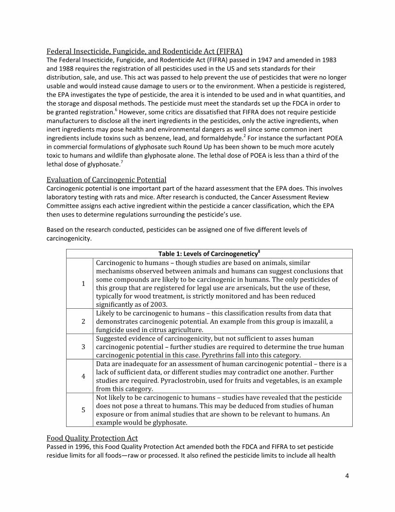
Federal Insecticide, Fungicide, and Rodenticide Act (FIFRA) The Federal Insecticide, Fungicide, and Rodenticide Act (FIFRA) passed in 1947 and amended in 1983

and 1988 requires the registration of all pesticides used in the US and sets standards for their

distribution, sale, and use. This act was passed to help prevent the use of pesticides that were no longer

usable and would instead cause damage to users or to the environment. When a pesticide is registered,

the EPA investigates the type of pesticide, the area it is intended to be used and in what quantities, and

the storage and disposal methods. The pesticide must meet the standards set up the FDCA in order to

be granted registration.6 However, some critics are dissatisfied that FIFRA does not require pesticide

manufacturers to disclose all the inert ingredients in the pesticides, only the active ingredients, when

inert ingredients may pose health and environmental dangers as well since some common inert

ingredients include toxins such as benzene, lead, and formaldehyde.2 For instance the surfactant POEA

in commercial formulations of glyphosate such Round Up has been shown to be much more acutely

toxic to humans and wildlife than glyphosate alone. The lethal dose of POEA is less than a third of the

lethal dose of glyphosate.7

Evaluation of Carcinogenic Potential Carcinogenic potential is one important part of the hazard assessment that the EPA does. This involves

laboratory testing with rats and mice. After research is conducted, the Cancer Assessment Review

Committee assigns each active ingredient within the pesticide a cancer classification, which the EPA

then uses to determine regulations surrounding the pesticide’s use.

Based on the research conducted, pesticides can be assigned one of five different levels of

carcinogenicity.

Table 1: Levels of Carcinogeneticy8

1

Carcinogenic to humans – though studies are based on animals, similar

mechanisms observed between animals and humans can suggest conclusions that

some compounds are likely to be carcinogenic in humans. The only pesticides of

this group that are registered for legal use are arsenicals, but the use of these,

typically for wood treatment, is strictly monitored and has been reduced

significantly as of 2003.

2

Likely to be carcinogenic to humans – this classification results from data that

demonstrates carcinogenic potential. An example from this group is imazalil, a

fungicide used in citrus agriculture.

3

Suggested evidence of carcinogenicity, but not sufficient to asses human

carcinogenic potential – further studies are required to determine the true human

carcinogenic potential in this case. Pyrethrins fall into this category.

4

Data are inadequate for an assessment of human carcinogenic potential – there is a

lack of sufficient data, or different studies may contradict one another. Further

studies are required. Pyraclostrobin, used for fruits and vegetables, is an example

from this category.

5

Not likely to be carcinogenic to humans – studies have revealed that the pesticide

does not pose a threat to humans. This may be deduced from studies of human

exposure or from animal studies that are shown to be relevant to humans. An

example would be glyphosate.

Food Quality Protection Act Passed in 1996, this Food Quality Protection Act amended both the FDCA and FIFRA to set pesticide

residue limits for all foods—raw or processed. It also refined the pesticide limits to include all health

5

risks rather than simply cancer, and to take into consideration the higher risks that children and infants

face. This act also sharply reduces the amount of time between when a pesticide is banned to the time it

must be removed completely from use (from 10 years to 14 months).2

Clean Water Act The Clean Water Act (CWA), originally passed in 1948 and expanded in 1972 with amendments in 1977

is the primary federal law monitoring water quality which sets the structure for regulating

concentrations of pollutants in surface water supplies. Ground water is not described in this law. It

protects “navigable” water bodies by limiting point source discharges that manufacturers and other

facilities may make into surface water bodies with the goal of making them safe for fishing and

swimming.9 Non-point sources are more difficult to monitor and regulate, and the approach for this

involves education, technical assistance to manufacturers, and similar approaches. Water quality

standards specify water quality standards (WQS) for allowable pollutant levels that water bodies must

meet, involving total maximum daily loads (TMDLs).10

The basis of these standards is the protection of aquatic life as well as human health. Aquatic life must

maintain a certain quality of water, including sufficient oxygen and nutrient levels, limits on alkalinity,

dissolved solids, turbidity, dissolved metals, and other potential pollutants. pH must be in the range of

6.5 – 9. Temperature is species dependent for the aquatic life criteria. Human life criteria consider

pollutants effects upon humans and the environment.9

Safe Drinking Water Act This act was first passed in 1974 and amended in 1986 and 1996. It regulates drinking water quality in

public water supply systems as well as their sources. The EPA sets primary and secondary drinking water

standards that water treatment facilities must comply with before discharge to public water distribution

systems. These standards involve treatment processes that must be included as well as permissible

contaminant levels in the plant’s effluent. States may also set their own drinking water standards as long

as they are at least as stringent as the national standards.11

Under this portion of the law, both drinking water health regulations and advisories are made. The

National Primary Drinking Water Regulations (NPDWRs) specify maximum contaminant levels (MCLs) of

a contaminant that is the highest permissible and safe concentration in water discharged to public water

systems. These contaminants include microorganisms, disinfectants and byproducts, inorganic

chemicals, organic chemicals, and radionuclides. Many pesticides have specified MCLs, including alachlor

(0.002 mg/L), atrazine (0.003 mg/L) and glyphosate (0.7 mg/L).12 Potential health effects are included in

this analysis. Table 2 lists some of the organic chemicals’ MCLs listed by the EPA. The full list is shown in

Appendix A. Maximum contaminant level goals (MCLGs) are non-enforceable recommendations below

which there is no expected health effects.12

Secondary standards also exist which encompass aesthetic aspects or cosmetic effects. Drinking water

advisories are made, which provide information and about contaminants’ health effects upon humans.12

6

Table 2: Organic Chemicals’ MCL’s (Incomplete)12

Contaminant MCLG1

(mg/L)2

MCL or

TT1

(mg/L)2

Potential Health Effects

from Long-Term Exposure

Above the MCL (unless

specified as short-term)

Sources of Contaminant in

Drinking Water

Acrylamide zero TT8

Nervous system or blood

problems; increased risk of

cancer

Added to water during

sewage/wastewater

treatment

Alachlor zero 0.002 Eye, liver, kidney or spleen

problems; anemia; increased

risk of cancer

Runoff from herbicide used

on row crops

Atrazine 0.003 0.003 Cardiovascular system or

reproductive problems

Runoff from herbicide used

on row crops

Benzene zero 0.005

Anemia; decrease in blood

platelets; increased risk of

cancer

Discharge from factories;

leaching from gas storage

tanks and landfills

Benzo(a)pyrene

(PAHs) zero 0.0002

Reproductive difficulties;

increased risk of cancer

Leaching from linings of

water storage tanks and

distribution lines

Carbofuran 0.04 0.04

Problems with blood,

nervous system, or

reproductive system

Leaching of soil fumigant

used on rice and alfalfa

Carbon

tetrachloride zero 0.005

Liver problems; increased

risk of cancer

Discharge from chemical

plants and other industrial

activities

Chlordane zero 0.002

Liver or nervous system

problems; increased risk of

cancer

Residue of banned

termiticide

Monitoring Foods for Quality The Food and Drug Administration (FDA) and US Department of Agriculture (USDA) enforce the

tolerance limits for residues of pesticides left on foods that are sold for human consumption. The limits

are set by the EPA. If the residue concentrations are found to be greater than the allowable standards,

the food must be destroyed, which provides incentive for farmers to abide by the limits.13 More

recently, the EPA has increased the number of tests conducted on foods commonly eaten by infants and

children in attempts to more closely protect the more susceptible younger populations.14

7

International Legislation Internationally, the International Code of Conduct on the Distribution and Use of Pesticides was passed

in 1985 by the United Nations’ Food and Agriculture Organization (FAO) and revised many times since

then, the latest in 2002, to set voluntary standards for the use of pesticides. Though countries are not

obligated to abide by these standards, they help raise awareness of the potential consequences

associated with use of pesticides and serve as a reference that is considered the “globally accepted

standard for pesticide management”.1 National legislatures maintain the standards that each country

must abide by but in some cases, particularly in developing countries, monitoring compliance with laws

is difficult.

European Union Legislature More formally, the European Union (EU) has detailed legislation surrounding the use of pesticides in

member nations. In doing this, the EU has separated its legislation into two main divisions: the

classification and usage of pesticides, and the official maximum residue level for each compound. These

two divisions work together to set a standard for pesticide restriction in order to keep the general public

safe.

Classification and Usage The first initiative in which the European Union started to standardize the restriction and legislation of

pesticides occurred in 1993 when Directive 91/414 was passed by the EU. This directive stated that over

the next 14 years a council was to be created to review all pesticides, their uses and the products in

which they were found. The review would establish whether the pesticides and products were harmful

to the community and would either allow continued production of the pesticide or ban the product

and/or pesticide. This stemmed from concern regarding the effects of pesticides on the food market

both within and outside the European Union. 15

The classification of the pesticide would be based on information from manufacturers, regarding

pesticide efficiency, main purpose, and potential harm to humans and the environment. The

classification would simply list the chemicals followed by this information. The EU would then make a

decision to either ban or allow the continued production of this pesticide. This process, otherwise

known as risk assessment, took into account the possible damage the pesticide could present should

there be a contamination in the local water system. Risks to humans as well as the possible risks to the

environment and wildlife were of paramount importance. In December of 2008, the review process was

extended until 2010 and then later until 2012. Prior to this directive the legislature on pesticide

restriction was dealt with on the national level only.15

The next directive, Directive 2009/128/EC, was passed in November 2009 and states that each national

community will develop and/or adopt a National Action Plan. This plan would be used on the national

level to reduce the risk to human and environmental life when dealing with pesticide usage. The hope of

this Directive is to focus on the pesticide concentration in food products. The plan was passed in hopes

to advocate the research and development of new techniques and delivery methods.15

In May 2011, the Plant Protection Products Regulation Act established a list of approved chemicals and

products for use in the EU. This list shows the accepted purity, date of approval, as well as the expiration

of approval. Once a pesticide’s approval expires, the review committee reevaluates the chemical and

may either continue to approve the usage or ban the pesticide. Coinciding with Directive 91/414, a list

was also established which lists banned substances in the European Union.16

8

Maximum Residue Level The second division of the European Union’s pesticide legislation involves the investigation of each

pesticide in order to establish a maximum residue level. This maximum residue level is the maximum

concentration that is found in local crops. The European Union defines these levels as the “highest

possible level of a pesticide residue that is legally authorized in food and feed.” In September 2008, the

EU passed Regulation 396/2005. This regulation set a standard for maximum residue levels in all EU

governed states. This regulation was to ensure that a product would not be legal in one country and yet

above the maximum residue level in another community.17

Health Impacts and Toxicity In addition to the desired effects on targeted pests, pesticides can also have detrimental effects on

human health. Acute effects occurring within minutes or hours after a single exposure, as well as chronic

effects spanning multiple exposures and weeks to years can be sustained. Various mechanisms of

contact with the pesticide can lead to different symptoms. Chronic toxicity is much more difficult to

monitor and observe since the effects are widespread, and depend on individuals’ various degrees of

contact with the substance and the individuals’ own health affected by genetics and various other

factors, and may have synergistic effects with other substances or lifestyles the individual was exposed

to. Chronic effects include birth defects, tumor formation, cancer, blood disorders, and nerve disorders.

Both long and short-term effects are tested by subjecting test animals to concentrations of pesticides to

simulate human effects, either for short exposures or, in chronic tests, the equivalent of extended

exposures.

Toxicity Information Dermal contact is responsible for the majority (~90%) of pesticide poisonings, typically during pesticide

application, handling, or other routine uses.13 Ingestion and inhalation are the other means. The

seriousness of dermal exposure and the degree of the effects then depend on the rate of absorption of

the substance through the skin, the size of the area of skin exposure, the length of contact time, the

number and concentration of the substances that contacted the skin, and of course, the level of toxicity

of the pesticide(s). Pesticides that volatilize can be inhaled from the atmosphere. Eye irritation can also

result from direct contact with pesticides.

Acute toxicity levels are measured by the half lethal dose, or LD50: the dosage at which 50% of animals

exposed to the substance were killed. The lower the LD50 is for a particular pesticide, the greater the

toxicity. This acute toxicity level determines the type of labeling required for pesticide containers, to

help warn users of their dangers. Table 3 shows the acute toxicity level standards. Highly toxic pesticides

must have the words “danger” and “poison” displayed on them, as well as the universally understood

skull and crossbones picture. Only a few drops of highly toxic pesticides could be fatal for a 150-pound

person. Moderately toxic pesticides have “warning” labels and either slightly toxic or relatively non-toxic

pesticides read “caution.” Even pesticides classified as relatively non-toxic can still be hazardous if

proper care if not taken to use them as directed and avoid excessive exposure.18

9

Table 3: Acute Toxicity Measures and Warnings13

LD50 LD50 LC50

Categories Signal Word Oral

mg/kg

Dermal

mg/kg

Inhale

mg/l Oral Lethal Dose*

I Highly Toxic DANGER, POISON (skull &

crossbones) 0 to 50 0 to 200 0 to 0.2

a few drops to a

teaspoonful

II Moderately

Toxic WARNING 50 to 500

200 to

2,000

0.2 to

2.0

over a teaspoonful to

one ounce

III Slightly Toxic CAUTION 500 to

5,000

2,000 to

20,000 2.0 to 20

over one ounce to one

pint

IV Relatively Non-

toxic

CAUTION (or no signal

word) 5,000+ 20,000 + 20 +

over one pint to one

pound

* Probable for a 150 lb.-person.

To avoid excessive exposure and help protect against pesticide-induced health risks when handling

them, manufacturers recommend some levels of minimum person protective equipment (PPE) which

typically includes long pants and sleeves, shoes, gloves, and possibly safety glasses and a face mask for

more toxic pesticides.

Table 4 lists some common herbicides in use in the US, their active ingredients, and the acute oral and

dermal LD50 values. REI, or restricted-entry interval, is the amount of time necessary between the

application of the pesticide to crops and the safe reentry of humans into the area is permitted and is

also listed. This is a partial excerpt taken from a list of 77 pesticides for which LD50 values were

reported.18

Table 4: LD50 Concentrations and Restricted-Entry Intervals for Selected Herbicides18

LD50 Values (mg/kg) REI

Active Ingredient, Trade Name Use Category Oral Dermal (hours)

Acetochlor, Degree R 2,148 4,166 12

Acifluorfen, Blazer G 2,025 >2,000 48

Alachlor, Lasso, Partner R-12 Tech 930-1,350 13,300 12

Ametryn, Evik G 1,950 � 12

Asulam, Asulox G >5,000 >2,000 12

Atrazine, AAtrex R 1,869 >3,100 12

Bensulide, Prefar G Tech 271-1,470 � 12

Bentazon, Basagran G 2,063 >6,050 12

Bromoxynil, Brominal, Buctril G Tech 260 >2,000 12

Butylate, Sutan + G 4,500 >4,640 2

Carfentrazone-ethyl, Aim G 5,143 >4,000 12

Health Effects Organisms that come into contact with pesticides typically suffer negative health effects, either acute or

chronic, that have the potential to be very severe. As desired, pesticides are acutely toxic to pests and

10

work to inactivate them; thus this highly toxic nature can be expected to have similarly detrimental

effects on both animals and humans, varying with the length of the exposure and the dose of the

pesticide. These health effects can result from direct contact with pesticides, but also indirect contact

when an individual drinks contaminated water or consumes contaminated foods.

Bioaccumulation and Biomagnification Persistent pesticides that do not readily degrade can be stored within plants and later consumed by and

transferred to animals and humans. Since many of these pesticides can be fat-soluble, they accumulate

within fatty tissue of animals and humans. As subsequent animals consume the previous animals, the

pesticide components remain within the system. High concentrations of the pesticide are stored.

Moving up the food chain, organisms closer to the top have higher concentrations of these pesticides

within their tissues. This phenomenon of greater concentrations of pesticides with successively higher

levels on the food chain is called biomagnification. Population groups that consume large amounts of

fish and wildlife may be at increased risks of health consequences due to bioaccumulation of toxic

pesticide compounds.2

A group within the EPA focuses on persistent, bioaccumulative, and toxic (PBT) pesticides’ effects and

monitoring, since these pose serious health issues that remain for years.19 These Level 1 PBT pesticides

are aldrin, dieldrin, chlordane, DDT, mirex, and toxaphene; all highly chlorinated which degrade very

slowly.20

Short-Term Effects Humans that are exposed to large doses of pesticides even for short periods of time can experience

serious health effects. These may range from nausea and vomiting, too much more serious

consequences, even death, depending on the type of pesticide and the dosage. The individuals’ prior

health also plays a significant factor but high doses of pesticides can be fatal. Organophosphates, in

particular, tend to have extreme acute effects. According to the World Health Organization, 300,000

people die annually from pesticide poisoning worldwide, while a total of four million suffer other health

effects from some form of poisoning. This is often due to improper handling of pesticides and not

necessarily only due to the transport and transfer of pesticides in the environment.2 Neurological

disruptions including headaches, dizziness, nausea, vomiting, confusion, tremors, and convulsions are

possible, as well as eye, nose, mouth, and throat irritation.

Long-Term Effects Chronic exposure to pesticides can have a wider range of health effects. Pesticides have been linked to

many different types of cancers including lymphoma, leukemia, and brain, lung, and testicular cancer.

Breast cancer may be linked to pesticides since they tend to bioaccumulate within breast tissue but

further research must be conducted to definitively prove the correlation. Long-term exposure is also

responsible for causing sterility both in humans and in other animals. Miscarriages also have been linked

to pesticide exposure. Another disease that may be related to contact with pesticides is Parkinson’s

disease. With each of these long-term illnesses, identifying a definitive correlation between exposure to

a specific pesticide and the illness can be difficult since large sample populations may not be available,

and many other factors could play into the individual’s illness.2

Level 1 pesticides are all classified as probably carcinogens. Some have been linked to central nervous

system damage and neurological system disruption, damage to the liver, kidney, thyroid, reproductive

system, and digestive system. Some may cause neurological disorders in children whose mothers are

exposed during nursing or before giving birth. Many are suspected endocrine disruptors.20

11

Endocrine Disruptors Many different types of pesticides have been shown to affect the endocrine hormones, such as estrogen

and testosterone, as well as alter the reproductive systems or organs of animals. These endocrine

disruptors can affect many different types of organisms, such as fish, amphibians, birds, reptiles,

laboratory rats, and even humans. For example, male frogs that were exposed to atrazine were found to

turn into females from lack of testosterone. 75% of male frogs were emasculated and 10% were turned

into females. When these atrazine-induced females then mated and produced offspring, all offspring

were male, skewing the sex-ratio of frogs in that population.21

Research into the possible endocrine disruption in humans has yet to determine the long term potential

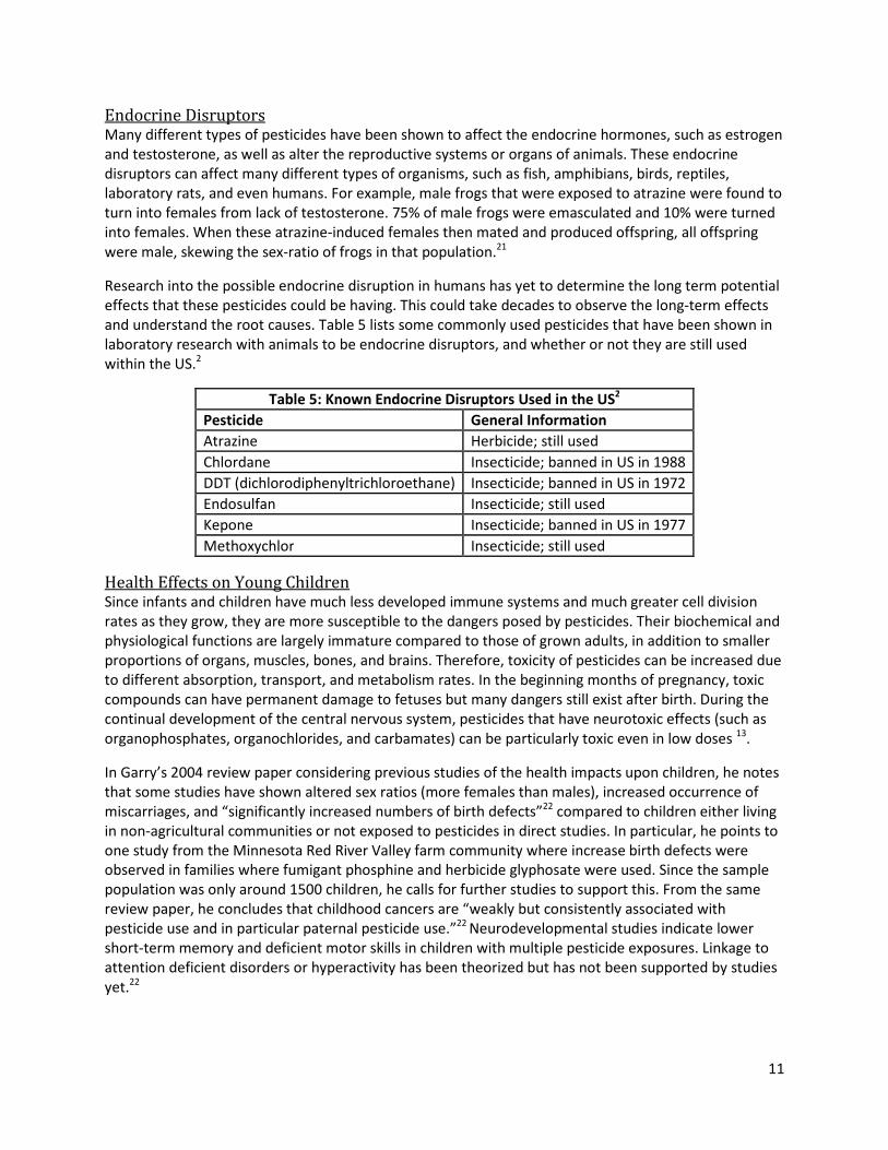
effects that these pesticides could be having. This could take decades to observe the long-term effects

and understand the root causes. Table 5 lists some commonly used pesticides that have been shown in

laboratory research with animals to be endocrine disruptors, and whether or not they are still used

within the US.2

Table 5: Known Endocrine Disruptors Used in the US2

Pesticide General Information

Atrazine Herbicide; still used

Chlordane Insecticide; banned in US in 1988

DDT (dichlorodiphenyltrichloroethane) Insecticide; banned in US in 1972

Endosulfan Insecticide; still used

Kepone Insecticide; banned in US in 1977

Methoxychlor Insecticide; still used

Health Effects on Young Children Since infants and children have much less developed immune systems and much greater cell division

rates as they grow, they are more susceptible to the dangers posed by pesticides. Their biochemical and

physiological functions are largely immature compared to those of grown adults, in addition to smaller

proportions of organs, muscles, bones, and brains. Therefore, toxicity of pesticides can be increased due

to different absorption, transport, and metabolism rates. In the beginning months of pregnancy, toxic

compounds can have permanent damage to fetuses but many dangers still exist after birth. During the

continual development of the central nervous system, pesticides that have neurotoxic effects (such as

organophosphates, organochlorides, and carbamates) can be particularly toxic even in low doses 13.

In Garry’s 2004 review paper considering previous studies of the health impacts upon children, he notes

that some studies have shown altered sex ratios (more females than males), increased occurrence of

miscarriages, and “significantly increased numbers of birth defects”22 compared to children either living

in non-agricultural communities or not exposed to pesticides in direct studies. In particular, he points to

one study from the Minnesota Red River Valley farm community where increase birth defects were

observed in families where fumigant phosphine and herbicide glyphosate were used. Since the sample

population was only around 1500 children, he calls for further studies to support this. From the same

review paper, he concludes that childhood cancers are “weakly but consistently associated with

pesticide use and in particular paternal pesticide use.”22 Neurodevelopmental studies indicate lower

short-term memory and deficient motor skills in children with multiple pesticide exposures. Linkage to

attention deficient disorders or hyperactivity has been theorized but has not been supported by studies

yet.22

12

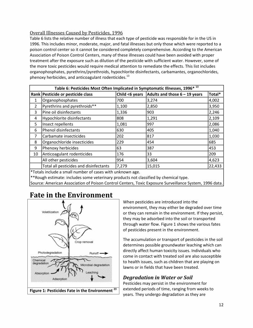
Overall Illnesses Caused by Pesticides, 1996 Table 6 lists the relative number of illness that each type of pesticide was responsible for in the US in

1996. This includes minor, moderate, major, and fatal illnesses but only those which were reported to a

poison control center so it cannot be considered completely comprehensive. According to the American

Association of Poison Control Centers, many of these illnesses could have been avoided with proper

treatment after the exposure such as dilution of the pesticide with sufficient water. However, some of

the more toxic pesticides would require medical attention to remediate the effects. This list includes

organophosphates, pyrethrins/pyrethroids, hypochlorite disinfectants, carbamantes, organochlorides,

phenoxy herbicides, and anticoagulant rodenticides.13

Table 6: Pesticides Most Often Implicated in Symptomatic Illnesses, 1996* 13

Rank Pesticide or pesticide class Child <6 years Adults and those 6 – 19 years Total*

1 Organophosphates 700 3,274 4,002

2 Pyrethrins and pyrethroids** 1,100 2,850 3,950

3 Pine oil disinfectants 1,336 903 2,246

4 Hypochlorite disinfectants 808 1,291 2,109

5 Insect repellents 1,081 997 2,086

6 Phenol disinfectants 630 405 1,040

7 Carbamate insecticides 202 817 1,030

8 Organochloride insecticides 229 454 685

9 Phenoxy herbicides 63 387 453

10 Anticoagulant rodenticides 176 33 209

All other pesticides 954 3,604 4,623

Total all pesticides and disinfectants 7,279 15,015 22,433

*Totals include a small number of cases with unknown age.

**Rough estimate: includes some veterinary products not classified by chemical type.

Source: American Association of Poison Control Centers, Toxic Exposure Surveillance System, 1996 data.

Fate in the Environment When pesticides are introduced into the

environment, they may either be degraded over time

or they can remain in the environment. If they persist,

they may be adsorbed into the soil or transported

through water flow. Figure 1 shows the various fates

of pesticides present in the environment.

The accumulation or transport of pesticides in the soil

determines possible groundwater leaching which can

directly affect human toxicity issues. Individuals who

come in contact with treated soil are also susceptible

to health issues, such as children that are playing on

lawns or in fields that have been treated.

Degradation in Water or Soil Pesticides may persist in the environment for

extended periods of time, ranging from weeks to

years. They undergo degradation as they are

Figure 1: Pesticides Fate in the Environment 23

13

metabolized and oxidized into potentially less-toxic substances, in some cases into only carbon dioxide

and any other elements in the base compound. Pesticides that readily undergo degradation are called

non-persistent. Recalcitrant pesticides are persistence and do not readily degrade. Some of the most

persistent pesticides include chlorinated hydrocarbons.2

Degradation can occur through three primary means. Microorganisms, particularly bacteria and fungi

within the soil or in water supplies can degrade compounds. Microorganisms harvest the carbon and

other organic components in pesticides as substrate and degrade the compounds through simple

chemical reactions. The rate of this degradation depends on a number of factors, including temperature,

oxygen content, pH, the amount of organics present in the oil, and the size of the microorganism

population. This degradation can be quite rapid, since microorganism populations can grow

exponentially in favorable conditions when substrate is available to them.9 Degradation can also occur

through chemical reactions independent of microorganisms. Chemical oxidation can also occur in the

absence of microorganisms or sufficient oxygen. One of the most common mechanisms of chemical

degradation is hydrolysis, or the breakdown when in contact with water.23 UV radiation from the sun can

also degrade compounds in surface water supplies or on the topmost layer of soil, called

photodegradation. This is limited to exposed areas, however, and occurs more commonly on leaves or

trees rather than when the pesticide is applied directly to the soil.24

Eventually, pesticides form residues when all of their original carbon has been oxidized to form CO2, a

process called mineralization. Secondary components formed during degradation are called metabolites,

and are specific to each type of pesticide. These metabolites that may persist longer than the parent

pesticide, may have lower activities than the parent and be less harmful. In other cases, however, the

byproducts formed may be more harmful and more persistent. These metabolites are the compounds

that are typically tested for in humans and other animals to determine pesticide presence.23

The commonly used pesticide atrazine provides a good example of the possible long-term effects of

pesticides in the environment. According to USEPA, the overall half-life of atrazine is 608 days, the water

half-life is 578, and the sediment half-life is 330 days. Field half-lives have been found to be between 13

and 261 days; variances were attributed to temperature differences and the assumption was made that

atrazine could remain longer in colder temperatures without degrading. A study in Oregon found the

half-life for atrazine on exposed soil was 87 days, in foliage was 13 days, and on leaves and leaf waste

was 66 days. On turf, the half-life is shorter (between 5 to 10 days). Since atrazine has a low adsorption

coefficient with many plants, it is likely to be washed into water sprays and may leach downward into

groundwater supplies. Transport into surface water supplies has been shown to be possible also.

Atrazine is mobile and persistent.17

Adsorption in Soil In general, pesticides can either accumulate in the top layers of soil if they have a high affinity for the

soil or are not highly water soluble, or they can leach downward and potentially into groundwater if

they are more water soluble or mobile. Highly mobile pesticides will have a lower residence time in the

soil, but then may be more likely to transfer to water supplies or contaminate other soil areas if they are

persistent. Bonding between soil and pesticide particles is dependent on the chemical and physical

properties of each species such as the charge of the pesticide as well as the charge of the soil.23 The

organic content of the soil is the greatest determining factor affecting the adsorption of pesticides in the

soil and may range from 0.1% to 90%, from desert sand to more organic soils.25 Sandy soils are less likely

to retain pesticides than other soils with high concentrations of organic matter or clay since organic soils

have greater surface areas and therefore more bonding sites for the pesticide to adsorb. Drier soils are

14

more likely to adsorb pesticides since water molecules do not preferentially block pesticides from

bonding.23 Adsorption coefficients for particular pesticides in certain soil types are necessary to

determine the transport of pesticides through soil.26 Pesticide adsorption in soil can also affect plant life,

since pesticides used to treat one type of pest can destroy desired plants that come into contact with

treated soil. In some cases, the adsorption into soils is considered during application of the pesticide and

higher concentrations are recommended for use in order to have the same effects. However, the

environmental fate of these pesticides used in high concentrations because they are known to be

mobile must be kept in mind.23 Table 7 reports the likelihood of groundwater contamination based on

pesticide and soil characteristics as well as the water volume that contributes to transport.24

Table 7: Groundwater Contamination Potential as Influenced by Water, Pesticide, and

Soil Characteristics24

Risk of Groundwater Contamination

Low Risk High Risk

Pesticide Characteristics

Water solubility Low High

Soil adsorption High Low

Persistence Low High

Soil Characteristics

Texture Fine clay Coarse sand

Organic matter High Low

Macropores Few, small Many, large

Depth to groundwater Deep (>100 ft) Shallow (<20 ft)

Water Volume

Rain/irrigation Small volumes at infrequent

intervals

Large volumes at frequent

intervals

Transport in Soil and Water There are five main ways in which pesticides can be transported in the environment after application:

runoff, leaching, absorption, volatilization, and crop removal. Many of these ways involve water

transport but all can contribute to movement into new environment. In many cases, multiple

environmental fate processes interact and lead to variable byproduct formation as well as transport.24

Runoff Runoff is the transport of pesticides in water above the earth’s surface that does not absorb downwards

into soil but instead flows over the surface of the earth due to gravity. Flooding, rainwater, or applied

watering can lead to runoff if the water added is greater than the amount that the soil can absorb. As

pesticides are dissolved in this water, they are carried along with it. The degree to which pesticides are

carried by the water depends on their solubility at that pH and temperature, the amount of vegetation

in the area that would potentially hinder the pesticide flow, and other factors.23

Leaching Leaching describes the transport of pesticides downward through the soil into the water table. This

movement depends on the chemical properties of the pesticide as well as of the soil type, as discussed

before, since strongly adsorbed compounds are less likely to undergo leaching. Water present within soil

can also affect leaching. Water may dissolve pesticides and carry them downward or into groundwater

supplies, contaminating them. This movement within water is dependent on the compound’s solubility

in water as well as the water flow patterns. The permeability of the soil itself, or how rapidly it allows

15

movement of water and pesticides through it, also affects leaching. Typically, pesticides leach downward

towards water tables. The depth of the water table affects how likely groundwater leaching will be. That

is, for a deep water table, the time that a pesticide needs to reach downward to the water table is

longer and provides more allowance for possible adsorption into the soil or degradation of the

compounds. Again, heavy precipitation or heavy water application can affect leaching since greater

amounts of water increase both the ability of pesticides to dissolve in larger quantities of water and also

increases the movement of the water itself. Different materials composing the soil layers also affect

leaching; for example, limestone dissolves more readily and allows water saturated with pesticides to

travel through sinkholes and enter groundwater.23

Absorption This is the transport of pesticides into plants cells. Once in the plants, pesticides may degrade or they

may remain within the plant for the length of the plant’s life. The toxins may then be transferred to any

organism that consumes the pesticide, contributing to bioaccumulation of the pesticide which can have

long-term effects through large spans of the food chain.2

Volatilization Volatilization is the transfer of pesticides from a solid or liquid phase into the gaseous phase. This then

allows for much more widespread possible movement of the pesticide since gases expand indefinitely in

open volumes and may be carried easily by air currents. These transported vapors can then damage

other plants, but also affect animal life and humans that inhale them. Pesticides with a high vapor

pressure are most likely to volatilize. Ambient temperature, pressure, and humidity also affect the rate

at which pesticides will volatilize.23

Crop Removal This is the movement of plants from their original location to other areas for use or sale, which can lead

to pesticide transport and contamination of new water supplies or other media. For example, the

washing of the plants that were treated with pesticides may remove the pesticides from the plants

themselves, as desired, but only transfers the pesticide to water used to clean the pesticides.23

Pesticides of Interest Three pesticides were studied specifically because of their wide use and occurrence in the environment:

alachlor, atrazine, and glyphosate.

Alachlor Alachlor, 2-chloro-2’-6’-diethyl-N-(methoxymethyl)

acetanilide, is an herbicide widely used in the United

States and other countries on crops such as corn,

soybeans, and peanuts. Figure 2 shows the chemical

structure of alachlor. It is an organochloride pesticide,

more specifically, a chloroacetanilide. Trade names include

“Lasso,” “Partner,” and “Bronco.” It is often found with

another member of the cloroacetanilide family,

metolachlor, with similar byproducts formed during

degradation. Alachlor is highly water soluble and therefore

poses a problem for water contamination and

transportation through ground and surface water

supplies.27 As of 1992, concentrations significantly greater than the MCL have been detected in at least

Figure 2: Chemical Structure of Alachlor

16

15 states by EPA’s Pesticide in Ground Water Database studies.28 According to the USEPA, the best

treatment technology available is granulated activated charcoal, which has been shown to remove it

down to the MCL.

Usage Alachlor was first registered for use in 1969. It is primarily used for broadleaf weeds and grasses.28 It

mixes well with other pesticides and is therefore commonly found in conjunction with others such as

atrazine, glyphosate, trifluralin, and imazaguin. Alachlor is heavily used in the Midwest of the US,

particularly Illinois, Indiana, Iowa, Minnesota, Nebraska, Ohio, and Wisconsin.28

The solubility of alachlor in water is 242 mg/L at 25°C.29

Legislation The maximum contaminant level acceptable in drinking water has been set at 0.002 mg/L (2 ppb) by the

USEPA. The maximum contaminant level goal is set at zero. It began being regulated under the Safe

Drinking Water Act in 1992.30

As of 1986, the Department of Agriculture, Trade, and Consumer Protection (DATCP) classified alachlor

as a priority pesticide because of its “high use, high leach, and detection.” This indicates that not only is

it a problematic issue in terms of environmental damage and in magnitude since it is widely used, but it

is also difficult to identify contaminated areas.27

Alachlor use in the European Union has been banned since 2006 due to known hazards to human health

and the environment.31

Health Implications Alachlor has an acute toxicity rating of slightly toxic (category III). The oral LD50 is 1350 milligrams per

kilogram of body mass, the dermal LD50 is 4982 mg/kg, and the inhalation LD50 is greater than 4.67

milligrams per liter of air.31 According to the EPA, individuals who repeatedly are exposed to

concentrations of alachlor higher than the MCL may experience health complications including liver

problems, eye problems, kidney problems, or spleen problems. They may also experience anemia.

Alachlor has not yet been conclusively evaluated for the EPA based on its carcinogenic potential for

humans. It has, however, been categorized as a probable human carcinogen (Group B2) based on animal

studies.32

European studies have classified alachlor into carcinogenic category 3, which include substances that

cause concern for humans due to potentially carcinogenic effects but for which insufficient data is

available so no complete conclusions can be made. When byproducts are formed during degradation, it

is “extremely unlikely” that an active metabolite of alachlor would lead to cancer but it cannot be

completely out ruled.31 There is similarly no conclusive data for possible endocrine disruption.31

Degradation Degradation of alachlor, like other pesticides, varies in different environmental conditions. Surface

water, soil, and groundwater degradation rates vary. Furthermore, degradation during transport

conditions complicates the identification of degradation products since new compounds can be

introduced from passing environments during transport. Biodegradation and chemical oxidation

produce similar byproducts for alachlor, called metabolites. According to the USEPA, at concentrations

between 1 and 5 ppb, higher temperatures led to greater degradation rates.30

17

The primary degradation that alachlor undergoes has been shown by many studies to be biodegradation

by aerobic microorganisms in soil. Thus the majority of degradation occurs in soil. Since alachlor is

largely water soluble, these byproducts may then transfer into groundwater supplies where they can

retained for extended periods of time since the half-life in groundwater has been proposed to be

between 808 and 1518 days by one study33 and 320 to 324 by another.34 Degradation occurs primarily in

soil or in surface water supplies, but not once the compounds have reached ground water.35

Byproducts Alachlor forms a large number of byproducts when degraded through different mechanism. A 1995

study by researchers at UMass detected 20 degradation products found in groundwater. The identities

of many products were confirmed with standards either purchased or synthesized with great purity, but

many, including the two most abundant compounds, were not identified definitively and were classified

only as “alachlor related”. A structure was proposed for one. In this study, four wells near a

Massachusetts corn field were sampled for concentrations of alachlor and related compounds at two

intervals, the second 30 months after the first. The same compounds were detected in both studies

(with one exception), demonstrating the long half-life and low rate of degradation once reaching ground

water. Interestingly, in one of the wells, no alachlor was detected but byproducts that were detected

were well over the MCL of 2 ppb demonstrating that byproducts may be a more significant issue than

the parent compound in some cases. The concentrations of each byproduct ranged from less than 2

nanograms per liter up to 410 nanograms per liter. In all monitoring wells, the total concentration of

byproducts was at least two times the concentration of alachlor detected, indicating that byproducts

form in significant concentrations. One byproduct that was reported in other studies but not found by

the researchers in Massachusetts were [[(2-6-diethylphenyl)methoxy]-methyl)amino]-2-oxoethane

sulfonate (ES).35

ES and 2-hydroxy-2,6-diethylacetanilide, 2’,6’-diethylaniline (DEA) have been identified by other studies

as two of the major alachlor degradation byproducts. A 1992 study focusing on ES studied 11 ground

and surface water sources in Indiana and Ohio and found concentrations ranging from 0.6 to 74 ng/L in

9 of these locations, below the MCL for alachlor.36 No MCLs have been set for alachlor byproducts. ESA,

the sulfonic acid analog of ES, was detected along with DEA by a study of 303 near-surface aquifers in

the US. The concentration of ESA was significant and greater than that of the parent compound found

alongside it. DEA was also detected frequently in this study but at lower concentrations.37 DEA was

found in many other studies and is highly water soluble, which presents a potential risk to ground

water.38

These and other studies have demonstrated that the concentrations of byproducts can be significant. In

terms of the toxicity of the byproducts themselves, each must be evaluated individually to truly

determine the potential harmful effects. This has not been fully investigated for all byproducts since

many remain unidentified.

In the following research, byproducts for alachlor will not be investigated due to time and detection

limitations presented by the wide range of byproducts that may be formed.

Persistence and Toxicity of Byproducts A structural isomer of ES was shown by the Monsanto Company to have a half lethal dose of over 5000

mg/kg from short-term animal testing. It was reported to be non-mutagenic and to not bioconcentrate

or undergo significant metabolic transformations when consumed by animals. As such, ES is not a very

toxic byproduct of alachlor.36 Out of the wells from the UMass study that showed ESA concentrations

above 0.10 micrograms per liter, 90% of them retained concentrations above this level during annual

18

subsequent samplings. ESA is therefore persistent, like its analog ES, but also remains relatively non-

toxic and not problematic though certainly abundant and persistent.37

DEA is water soluble and therefore mobile. However, in general, researchers at UMass comment that

the cleavage of the methoxymethyl group of alachlor may translate into detoxification. They point to

studies performed by Jacobsen et al that show that in mice, formaldehyde is liberated from the

methoxymethyl (MOM) group. If separated, the MOM-free degradation product would provide less

potential for formation of formaldehyde and as such have a powerful mutagenic potential.35 Another

study by Tessier showed that two compounds without the MOM group, 2-chloro-2’,6’-diethylacetanilide

and 2-hydroxy-2’,6’-diethylacetanilide were only weakly mutagenic to Salmonella strain TA100.

Therefore, although the specific toxicity of DEA has not been tested and a similar situation exits for the

numerous other byproducts of alachlor, the toxicity of compounds with a cleaved MOM group can be

considered low. Further studies are required to confirm this hypothesis proposed by researchers at

UMass.35,39

Atrazine Atrazine is an organochloride herbicide, often used in the

Midwest. Figure 3 shows the chemical structure. Atrazine

is found in the form in of a white crystalline solid. The

IUPAC name for atrazine is 2-chloro-4- (ethylamino)-6-

(isopropylamino)-s-triazine. The chloro refers to the

chlorine attached on the top of ring which identifies

atrazine as an organochloride pesticide. The ethylamino

and isopropylamino both refer to the two amino sites on

the molecule signified by the side chains of nitrogen. The

center ring made up of doubled and single bonded

nitrogens is also called a triazine ring with the ‘s’ detailing the specific configuration of said ring. The

configuration of the inner ring is that of a 1-3-5-trazine ring. That is, the nitrogen appears at the 1, 3 and

5 position in the ring.

Usage Atrazine is used worldwide as an herbicide. More specifically, atrazine is often used on field corn. In the

US, the EPA reports that 75% of field corn acreage grown in the U.S. is treated with atrazine making it

the most heavily used herbicide in the US. Typical methods of delivery for this pesticide include many

different forms of sprayers, aircraft and tractor delivery. 40

Legislation In the United States and the international community, atrazine has been labeled as a dangerous

herbicide. The process and time it took different communities to reach this conclusion was very

different. In the United States the first step in regulating atrazine use took place in 1974 when the Safe

Drinking Water Act set the MCL for atrazine at 3 ppb (parts per billion) in drinking water.41

In 1991, communities in Wisconsin noticed a large spike in atrazine concentration in their drinking

water. This examination led to the Wisconsin Atrazine Rule, which demands that no atrazine be used in

any areas that contain more than the allowed 3 ppb concentration in the drinking water in order to

avoid further increase of concentrations. The rule also only allows the use of atrazine from April 31st to

June 31st. The time restriction was implemented in order to greatly reduce the amount of atrazine used

on crops and therefore the amount of atrazine that could potentially infiltrate the local watersheds.

Shortly following the Wisconsin Rule, the federal government made steps to officially recognize atrazine

Figure 3: Chemical Structure of Atrazine

19

as a harmful contaminate and ban purchase of the pesticide from any persons other than licensed

applicators.40 It wasn’t until 1998, however, that the U.S. classified atrazine as a potential human

carcinogen42. Two years later, the EPA made an announcement that atrazine will be regulated at the

highest standards in the agency. In 2002, a startling discovery was made that atrazine, in far lower levels

than was set by the EPA, was causing the emasculation of frogs. Because of this discovery, the EPA was

sued that year by the National Resources Defense Counsel for not having stricter guidelines on a clearly

dangerous chemical. In the US today, the last evaluation of the threat of atrazine was conducted in 2003

although discussion within the EPA are said to have taken place in 2010 and are to continue in 2011.

These discussions could potentially add/loosen restrictions on atrazine use based on any up and coming

environmental data.40, 42

The toxicity of atrazine was realized much more quickly in Europe. In 1991 both Italy and Germany

banned use of atrazine. The European Union followed suite in 2004 with the banning of Atrazine for all

countries that are members of the union. One can deduce that regulation was delayed as long as it was

in the United States due to the incredible demand and dependency of the pesticide in the Midwest.42

Health Implications Analyzed by a research department at Cornell University, atrazine is classified as slightly to moderately

toxic.43 In studies made by the same research group, atrazine was found to cause skin irritation,

vomiting, diarrhea, stomach pains, muscle spasms and hypothermia. While there are numerous acute

symptoms of atrazine poising, the chronic toxicity is more severe. In one study, rats that were given a

steady dosage of twenty milligram of atrazine per kilogram of body mass (mg/kg) for six months showed

severe paralysis and respiratory damage. Forty percent of that sample population died within those first

six months of exposure. Rats exposed to a lower concentration of five mg/kg showed a strong reduction

in growth over six months. Among these symptoms, atrazine was shown to affect many different species

in many ways including having reproduction effects, teratogenic effects, mutagenic effects, carcinogenic

effects and organ toxicity.43

Degradation While the solubility of atrazine (33 mg/L) is relatively low in water, the half-life of the chemical is very

long, with aqueous samples lasting more than 60 days to 100 days. The actual degradation of atrazine is

due to chemical hydrolysis followed by degradation by microorganisms in the soil. As is common with

most pesticides, degradation occurs faster in non-neutral pH water and noticeably slower in pH neutral

water. The addition of humic material has also been noted to rapidly increase the degradation. Figure 4

depict the difference pathways in which atrazine would degrade.44

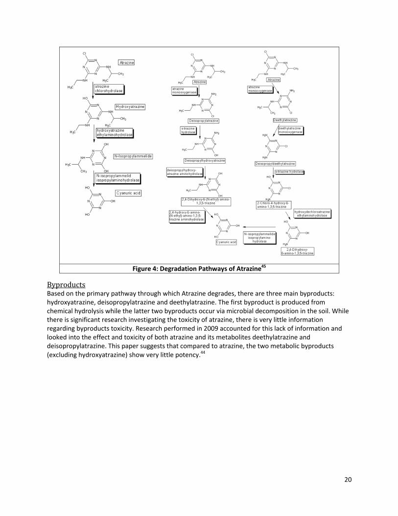
20

Figure 4: Degradation Pathways of Atrazine45

Byproducts Based on the primary pathway through which Atrazine degrades, there are three main byproducts:

hydroxyatrazine, deisopropylatrazine and deethylatrazine. The first byproduct is produced from

chemical hydrolysis while the latter two byproducts occur via microbial decomposition in the soil. While

there is significant research investigating the toxicity of atrazine, there is very little information

regarding byproducts toxicity. Research performed in 2009 accounted for this lack of information and

looked into the effect and toxicity of both atrazine and its metabolites deethylatrazine and

deisopropylatrazine. This paper suggests that compared to atrazine, the two metabolic byproducts

(excluding hydroxyatrazine) show very little potency.44

21

Glyphosate Glyphosate, N-(phosphonomethyl)-glycine, is a broad-

spectrum, nonselective herbicide used to control

annual and perennial plants. It is often used in both

croplands and residential areas. Glyphosate is an

organophosphate compound, which are generally

highly acutely toxic to humans and wildlife alike. The

structure of glyphosate, shown in Figure 5, has several

dissociable hydrogen atoms, including the first

hydrogen on the phosphate group. The presence of

these groups suggest potential for chemically treating

glyphosate.46

Glyphosate was first discovered to have herbicidal properties by John Franz in 1970, while working for

the Monsanto Company. By 1973, the Monsanto Company was marketing its glyphosate-based

herbicide, under the trade name Roundup. As glyphosate is highly soluble in water (up to 12 grams per

liter at 25 degrees C), it poses a significant threat to water contamination and transport through ground

water. 47

Glyphosate is rated to be less dangerous than other

herbicides from the organophosphate family, which is

evidenced by its EPA Toxicity Class of III (on a 1 to IV

scale, where I is the most dangerous).46 However, studies

suggest that when combined with other ingredients, the

Roundup mixture may be considerably more toxic than

glyphosate alone. The chemical surfactant used in the

commercial formulation, polyoxyethylated tallow amine

(POEA), has garnered attention recently, for causing damage and cell death to human cells. The

structure of POEA can be seen in Figure 6. Currently, because it is listed as an inert ingredient of

glyphosate formulations, POEA is not regulated under environmental laws.47

Usage Glyphosate is one of the most abundantly used pesticides in the United States. In 2007, the EPA

estimated that the agricultural market within the US was using up to 185 million pounds of glyphosate

per year. Additionally, as of 2005, genetically altered glyphosate resistant crops accounted for

approximately 75% of all genetically modified crops.48 Glyphosate is still legal throughout the world,

despite mounting evidence of the toxicity of its formulations.

Health Implications The LD50 of glyphosate in rats is 4,320 mg/kg.49 The Monsanto Company lists the LD50 as 5,600 mg/kg. In

2010, a European Food Safety Authority (EFSA) conference assessed the health effects of glyphosate

exposure as well as the health risks of genetically modified food and crops. One finding that came out of

this was that in human cells, Roundup is capable of causing total cell death within 24 hours of contact.47

Glyphosate acts as an enzyme inhibitor, and when applied to plants, it cuts off the shikimic acid

pathway, which does not exist in humans. However, this pathway is rather specific in action–it is the

method with which phenylalanine and tryptophan are consumed in plants and microorganisms—and

Figure 5: Chemical Structure of Glyphosate

Figure 6: Chemical Structure of POEA

22

while the shikimic pathway does not exist in humans, glyphosate does prevent the binding of

phosphoenol pyruvate from binding to enzymes. Phosphoenol pyruvate is a metabolite that is present in

all living organisms, and therefore, glyphosate has the potential to interfere with other metabolic

pathways.48

In an EPA study, data suggested that glyphosate can cause birth defects in certain test subjects. In this

study it was found that the effects of glyphosate on pregnant rats included “diarrhea, decreased weight

gain, nasal discharge. . .death of mothers, and kidney and digestive disorders”. 48 In 2009, Andres

Carrasco, an Argentinian government scientist, released his finding that exposure to glyphosate

herbicides caused malformations in frog and chicken embryos. However, his tests were conducted with

considerably lower concentrations of glyphosate than used in agricultural spraying. Malformations in

frog and chicken embryos were seen in samples which were injected with 2.03 mg/kg of glyphosate. The

maximum limit of residual glyphosate in soy in the European Union is 20 mg/kg, nearly 10 times higher.

Carrasco stated that people living in areas dependent on genetically modified soy crops had been

reporting problems in 2002, two years after the implementation of genetically modified crops in

Argentina. In April 2010, a survey of the population of La Leonesa and other areas of Argentina in which

genetically modified crops are harvested revealed that the childhood cancer rate had tripled in the

previous ten years; the rate of birth defects also increased four-fold.51 This information may indicate

severe health effects at concentrations much lower than the tests were conducted at.

An epidemiological study of Ontario farming populations showed that exposure to glyphosate through

application to crops nearly doubled the chances of late spontaneous miscarriages. Professor Eric-Giles

Seralini from Caen University has shown that glyphosate is toxic to human placental cells, killing a large

proportion of cells after an 18 hour exposure to concentrations well below agricultural use.49

Additionally, glyphosate interacts with the active site of the enzyme aromatase, which is responsible for

making estrogen. The interaction between glyphosate and aromatase was minimal unless a surfactant

was present. After 18 hours of incubation with a Roundup solution, enzyme activity had been inhibited.

The inhibition can be directly associated with a decrease in mRNA synthesis, which suggests that

Roundup decreases the rate of gene transcription.

Health Implications of POEA While glyphosate on its own is not acutely toxic, it is likely that the most common formulations of the

pesticide, such as Roundup, are more toxic than glyphosate itself. Roundup, one of the most common

implementations of glyphosate in pesticide use, includes a surfactant, called polyoxy-ethyleneamine

(POEA), which is used to prevent the chemical from forming droplets and rolling off the leaves on which

it is sprayed. Ethylated amines are significantly more toxic than glyphosate; they are irritants to the

eyes, respiratory tract, and the skin, and can contain dioxane contaminants, which are suspected of

being carcinogenic. The Food and Agriculture Organization of the United Nations has set standards of 1

ppm of 1,4-dioxane in formulations, which may be present in POEA surfactants.52 Additionally, new

research shows that commercial Roundup caused liver damage in rats. In this study it was found that

glyphosate and its surfactant in Roundup acted in synergy to increase the damage to the liver. It was

theorized as early as 1988 that the toxicity of POEA was much greater than that of glyphosate alone. The

acute lethal dose of POEA is “less than one third that of roundup and its active ingredient.” The lethal

dose of POEA is approximately 1200 mg/kg, compared to the 4,320 mg/kg reported for glyphosate.7

In the environment, it has been observed that POEA is more toxic than glyphosate. This is in part due to

the fact that POEA is more toxic in alkaline water than in acidic water, and therefore, the relative

potency of the chemicals is pH dependent.53 Data comparing the ecological toxicities of glyphosate,

POEA, and Roundup can be seen in Table 8.52

23

Legislation Glyphosate has garnered significant legal attention throughout the years. In 1996, the Monsanto

Company was accused of false advertising in regards to the safety of its product. Again in 2007, the

company was convicted of false advertising, having stated that their product left the soil clean after use.

The second case began in 2001 with the basis that glyphosate is both dangerous for the environment

and toxic to aquatic organisms. Additionally, the United States EPA has caught scientists deliberately

falsifying test results for Monsanto studies of glyphosate.54

In the United Kingdom, glyphosate is the most frequent cause for complaint recorded by the Health and

Safety Executive’s Pesticides Incidents Appraisal Panel. Between 1990 and 1995, there were 33

complaints recorded, as well as 34 poisonings involving glyphosate. Within the United States and in

other countries, glyphosate has frequent detrimental health effects. In California, it is the most

commonly reported cause of illness or injury to workers from pesticides. However, glyphosate is not yet

banned in any country.55

Degradation The degradation pathway for glyphosate in the environment can be seen in Figure 7.

Table 8: Estimates of Relative Potency of Toxicological Interaction of Glyphosate and POEA52

Observed LC50 values

Species Glyphosate POEA Roundup Relative Toxicity

pH 2

Rainbow Trout 240 0.65 2 369.2

Bluegills 220 1 2.6 220

pH 6.5

Rainbow Trout 140 7.4 10.8 18.9

Bluegills 140 1.3 6 107.7

pH 7.2

Rainbow Trout 140 2 11.8 70

Bluegills 140 3 7.1 46.7

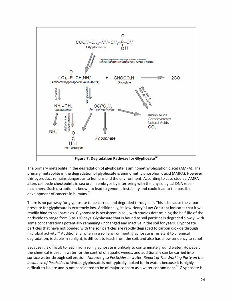
24

Figure 7: Degradation Pathway for Glyphosate52

The primary metabolite in the degradation of glyphosate is aminomethylphosphonic acid (AMPA). The

primary metabolite in the degradation of glyphosate is aminomethylphosphonic acid (AMPA). However,

this byproduct remains dangerous to humans and the environment. According to case studies, AMPA

alters cell cycle checkpoints in sea urchin embryos by interfering with the physiological DNA repair

machinery. Such disruption is known to lead to genomic instability and could lead to the possible

development of cancers in humans.52

There is no pathway for glyphosate to be carried and degraded through air. This is because the vapor

pressure for glyphosate is extremely low. Additionally, its low Henry’s Law Constant indicates that it will

readily bind to soil particles. Glyphosate is persistent in soil, with studies determining the half-life of the

herbicide to range from 3 to 130 days. Glyphosate that is bound to soil particles is degraded slowly, with

some concentrations potentially remaining unchanged and inactive in the soil for years. Glyphosate

particles that have not bonded with the soil particles are rapidly degraded to carbon dioxide through

microbial activity.52 Additionally, when in a soil environment, glyphosate is resistant to chemical

degradation, is stable in sunlight, is difficult to leach from the soil, and also has a low tendency to runoff.

Because it is difficult to leach from soil, glyphosate is unlikely to contaminate ground water. However,

the chemical is used in water for the control of aquatic weeds, and additionally can be carried into

surface water through soil erosion. According to Pesticides in water: Report of The Working Party on the

Incidence of Pesticides in Water, glyphosate is not typically looked for in water, because it is highly

difficult to isolate and is not considered to be of major concern as a water contaminant.52 Glyphosate is

25

highly soluble in water, with up to 11,600 ppm dissolving at 25 degrees C. Its hydrolysis half-life is

greater than 35 days, as glyphosate shows little propensity towards hydrolytic decomposition. Studies

suggest that its loss from water is due to sediment adsorption and microbial degradation. Therefore, the

degradation of glyphosate in water is slower than that of glyphosate in soil, as there are fewer

microorganisms in water to carry out the chemical pathways. However, fish and aquatic life are more

sensitive to glyphosate and its formulations than mammals and birds. Higher water temperatures and

pH levels have been observed to increase the toxicity of these compounds.7

Methods for Pesticide Removal from Water Pesticides can degrade in the environment through microbial decomposition, UV photolysis, chemical

oxidation, or hydrolysis. The following treatment techniques may be employed in wastewater and

drinking water treatment facilities to actively reduce pesticide concentrations prior to human

consumption or discharge to the environment.

Activated Carbon Adsorption In modern day water treatment, activated carbon is one of the most common techniques used by both

large and small treatment facilities. Activated carbon is very popular throughout industry for various

reasons including its low price, ease of use, and the limited machinery required. The mechanism in

which activated carbon purifies water is adsorption, where the pesticide or contaminant associates with

the porous carbon surface. Activated carbon offers high surface area for adsorption. While only being as

large as a grain of sugar, the high porosity of an activated carbon grain yields a very large surface area

for adsorption to occur. In fact, studies show that activated carbon can have a surface area of 500 m2

per gram. While the most common form of activated carbon is a black powered substance made from

coal, activated carbon can also be made from wood or coconut shells. The production of activated

carbon requires the intense burning of the raw material: coal, wood or coconut shells. Once sufficiently

burned, the ash is then activated using compounds such as zinc chloride or calcium chloride. These

chemical activate the ash by creating pores inside each individual ash particle.56

Types of Activated Carbon There are two main types of activated carbon. Powered activated carbon (PAC) has a much smaller

particle size and in turn has a low initial cost. Manufacturing costs are lower due to the small size.

Unfortunately the size is PAC’s greatest detriment. Due to the small size, powdered activated carbon is

known to clog machinery and other filters throughout a plant. Conversely, granular activated carbon

(GAC) has a much larger particle size and a higher initial cost. The advantage of using GAC is the ability

to reuse it. GAC particles are large enough that when the activated carbon reaches its breakthrough

point and is saturated, the particles can be recovered and the regenerated. Regeneration effectively

destroys contaminants and allows the GAC to be reused in the process. 57

Mechanism One common misconception regarding activated carbon is the difference between absorption and

adsorption. While many techniques utilize absorption, a process in which material is transferred into a

solid, activated carbon utilizes adsorption. The contaminant in the water sticks onto the wall of this

carbon. This adsorption mechanism is broken into three main parts. The contaminant first adheres to

the exterior surface of the activated carbon particle. Due to equilibrium, the process by which a particle

will travel from high to low pressure, the contaminant moves along the wall to larger pores located

deeper inside the activated carbon particle. The third stage of the mechanism includes the contaminant

coming to a final resting place on the inner surface of the grain of activated carbon. This process

continues until a no more contaminants can be adsorbed by the activated carbon. The maximum

26

adsorption can vary from substance to substance and is also directly affected by type of activated

carbon, temperature, pH and contact time.58

Figure 8: Activated Carbon Adsorption Process and Mechanism48

Figure 8 depicts the process by which chemicals travel into the porous piece of carbon. In step one, the

particle is in solution. For this figure, it can be assumed that the pressure in the solution is higher than

that of the inside of the carbon particle. In step two the particle is drawn into the pores of the activated

carbon due to the low pressure inside the pore. Once again this is the particle being brought to

equilibrium. In step three the particle is fully inside of the particle but has yet to find the lowest pressure

area. Step four involves the particle traveling further inside the pore and coming to rest at a wall, thus

reaching equilibrium.58

Economics Traditionally, PAC has been used in smaller facilities where the capital cost drives the demand. Because

of the GAC’s high capital cost but low difference, the actual particle size also impacts the choice of which

form to use. This consideration takes into consideration the types of equipment found downstream of

the filtration process. Due to the small particle size, PAC requires more involved filtration systems and

can potentially damage precision equipment downstream. GAC is therefore more commonly used.59

Modeling Adsorption with Activated Carbon One common way to model the adsorption of activated carbon is via the Freundlich model. In this

model, the following equation is used to predict specific parameters in the adsorption mechanism.

�

�� � ∗ ��

�

Where:

� � ��� �� ������� ����

� � ��� ���� �����

� � ������������ �����

� � ������������ �����

�� � ������������ �������� � �� ����

27

Using this equation, a log-log graph such as Figure XX can be formed in order to ascertain the

experimental constants. The goal of using this model is to ascertain the experimental constant (K/n).

With this constant one can theoretically find the mass of adsorbent needed to dissolve a certain

percentage of pesticide. Conversely, this model can accurately calculate a certain amount of pesticide an

adsorbent material can extract form a solution. In order to find the constant, one must experimentally

mix a mass of activated carbon and measure its resulting adsorption rate. With this rate one can get the

resulting amount of pesticide, Ce, left in the solution. With values experimentally found, a log-log graph

can be created and the resulting constants can be calculated. Experimental constants are specific to that

particular contaminant and form of activated carbon and in turn can be used to theoretically obtain

adsorption information. When plotted correct, as shown in Figure 9, the graph should show a linearly

increasing line.60

Figure 9: Sample Freundlich Isotherm Curve60

Chlorination Chlorination is a common technique used in water treatment facilities to deactivate undesired

microorganisms as well as reduce some pesticide concentrations through chemical oxidation. Chlorine

reacts with a number of species, including bacteria, viruses, nitrogen, hydrogen sulfide, cystide,

cyanides, phenols, and other organics through disinfection and oxidation.61 According to the World

Health Organization (WHO) in 2004, “chlorine is [the] most widely and easily used [disinfectant], and the

most affordable of the drinking water disinfectants.” Similarly, it is an affordable oxidant.62

Chlorine can be used in a number of forms to treat drinking water. Concentrations of either pure

chlorine or chlorine compounds are added to water supplies and are termed either free or combined

chlorine. Free chlorine is either in the form of pure chlorine gas Cl2 dissolved in water, hypochlorous acid

HOCl, or the hypochlorite ion OCl- which is formed because hypochlorous acid is a weak acid that

dissociates based on pH. 61At pH levels between 6-9, less than 1% of the available chlorine will be in the

pure form and will instead have hydrolyzed rapidly in water. This hydrolization is nearly instantaneous at

25°C and takes a few seconds at 0°C. Hydrolization Reactions 1 and 2 are shown here. Hypochlorous acid

is a stronger disinfectant than the hypochlorite ion, but the ion is a stronger oxidant. Therefore, pH

levels greater than the pKa of 7.6, the hypochlorite ion is dominant and conditions are more favorable

for oxidation.63

28

�� !"# + % & → %&�� + %( + ��) (Reaction 1)

%&�� + % & ↔ &��) + %+&( (Reaction 2)

Chlorine referred to as combined is in the form of chloramines, which form because of reactions with

ammonia present in natural water supplies at pH levels below 7. These include monochloramine,

dichloramine, and trichloramine, though only the first two are active oxidants. Once trichloramine is

formed, the chlorine no longer has the potential to degrade carbon compounds. Chloramines are more

stable and are therefore more often used to maintain concentrations within a water distribution

system.64

Chlorine is most commonly added to water either in the form of pure chlorine gas or in the form of a

sodium hypochlorite, or simply hypochlorite, also known as bleach. Calcium hypochlorite, the form of

chlorine used in swimming pools, is more concentrated and may also be used.64

Mechanism There are three general pathways that chlorine can react with substrate in water: oxidation, addition,

and substitution. Chlorine reacts with organic material through combinations of these pathways

depending on the material in the water.65

These chlorine compounds that are added to water have the potential to oxidize substrate. However,

many competing reactions occur that demand consideration when treating for pesticides.

Microorganisms are also deactivated by chlorine, though the underlying mechanism is still due to

oxidation of cell walls or other materials that destroys the organism. In order of their oxidation

potential, chlorine dioxide, then free chlorine, and then chloroamines are most effective. Ammonia

within water bonds with chlorine to form chloramines. Other contaminants within water may also

scavenge chlorine. Therefore, concentrations greater than the minimum chlorine demand calculated

using standard methods might be added to increase the potential for degradation of the target species.

Even in pure water to which concentrations of pesticides are added in a laboratory setting, rate

constants may limit the time required for oxidation based on concentrations. Excess chlorine may speed

up these reactions.9

Dosages The dose of any chlorine-containing compounds that is required to completely oxidize a pollutant can be

calculated by experiments comparing applied chlorine concentrations to the residual chlorine

concentrations in water samples with some chlorine demand. Methods described in Standard Methods

for the Examination of Water and Wastewater, published by the American Public Health Association,

American Water Works Association, and the Water Environment Federation, detail the determination of

the chlorine demand of a pollutant. The demand for specific chlorine forms (total, free, combined,

monochloramine or dichloramine) can be calculated depending on the test. Some of these tests include

amperometric titration with phenylarsine oxide titrant to determine the remaining chlorine after a

reaction period, titration with ferrous ammonium sulfate (FAS), or a colorimetric method comparing the

quality of samples to chlorine standards using a spectrophotometer.65 Studies have also been conducted

where molar ratios of the chlorine-containing species up to 100:1 relative to the amount of substrate in

water.66

Effectiveness The effectiveness of chlorine at oxidizing the desired pesticide depends on the water quality. If other

carbon sources are present in the water, these will exert a demand upon the chlorine and result in

29

competing oxidation and a lower overall pesticide reduction. pH levels and turbidity also impact the

distribution of available chlorine (free or combined).9 If the water contains sulfides, excess chlorine must

be used since this is a common reaction, which exerts a demand on the chlorine.

A study conducted in Spain measured the efficiency of various treatment techniques, chlorination

among them, and their efficiency at removing 44 different pesticides from water. Chlorination was

found to be 30% efficient at removing alachlor and 20% efficient for atrazine. Aluminum sulphate was

added as a coagulant at various doses but found to have no impact. A number of the 44 pesticides

studied did benefit from greater removal rates, up to 100% removal; an overall average removal of 60%

of the studied pesticides was found. However, the chlorine dose applied to these pesticides was the

minimum required to satisfy the chlorine demand. Higher concentrations may have contributed to

greater removal since impurities in the water may have exerted a chlorine demand, or the contact time

may have been insufficient for thorough oxidation.67

A study on glyphosate and glycine removal with chlorine used chlorine in molar ratios to substrate

ranging from 1:1 to 100:1 to observe products formed. With the 100:1 molar ratio assumed to be

comparable to the excess that water treatment facilities would use, glyphosate was totally degraded to

end products phosphoric acids, carbon dioxide, methanediol, nitrogen, and nitrate.66

Feasibility and Economics Chlorination is one of the least expensive treatment procedures. As such, it is commonly used in

wastewater and drinking water treatment facilities. It is essential that concentrations too great are not

consumed by humans and therefore controls and monitoring is necessary, which incur extra costs.

However, the treatment procedure itself is easy to implement and run, as well as low in installation and

chlorine costs.64

Dechlorination In water treatment facilities, residual chlorine concentrations must be reduced before discharge to

public water distribution systems in order to meet acceptable limits. While some chlorine must remain

in the water throughout the piping, excess can be dangerous. Many compounds that are formed from

chlorine, such as trihalomethanes (THMs), have been proven to be carcinogenic. Dechlorination is

achieved through use of sulfur dioxide, solutions of sulfite compounds, or granulated activated carbon

(GAC)61 Use of carbon adsorption is more expensive and would be used when total dechlorination is

required.

UV Photolysis Treatment of waters and wastewaters with UV is another technique used to degrade organic pollutants

and inactivate microorganisms to acceptable levels. UV light is a form of electromagnetic radiation in the

wavelength range of 100 to 400 nanometers. There are four classes: UV-A between 400 and 315 nm,

UV-B from 315 to 280, UC-C from 280 to 200, and vacuum UV from 200 to 100 nm. When used for water

treatment, low-pressure mercury lamps (LP-UV) generate UV at a wavelength of 253.7 nm and medium-

pressure lamps (MP-UV) generate UV and visible light in the 200-800 nm range. LP-UV lamps can

provide up to 0.4 kW while MP-UV lamps can provide up to 30 kW of power. 68

When used to degrade pollutants rather than targeting microorganisms, UV treatment is used as an

advanced oxidation process (AOP) inducing photodegradation of organic and inorganic contaminants in

water. The breakdown of pollutants into simpler compounds due to UV exposure is also called

photolysis. Since this occurs at a very low rate with UV alone, hydrogen peroxide is often added to

provide active hydroxyl radicals to bond to pollutants and oxidize compounds as a simultaneous and

30

parallel reaction to the photolysis. Semiconductor catalysts may also be added to encourage this process

through more rapid formation of active hydroxyl radicals or other radicals that attack pesticide

substrate; this is then called photocatalysis.69

UV treatment provides a number of benefits, including potentially complete oxidation of organics within

a few hours. In general, UV has the potential for many compounds to provide more successful removal

than other treatment procedures such as biodegradation, or activated carbon that involves a phase

transfer of pollutants rather than their actual destruction. Low concentrations may also be treated, in

the ppb range.69 Again, this varies by compound, but through the use of cost-effective catalysts that can

be adapted to specific systems, photolysis can be optimized.

Mechanism Photolysis is the chemical decomposition of compounds when a photon of light is absorbed. This

however, does not fully degrade them. This is often a successfully destructive pathway for pesticides in

surface water or on plant or soil surfaces that are therefore contacted by sunlight. The absorption of a

photon induces molecular excitation and elevation from a ground state to an elevated state. This excited

molecule may then undergo a degradation reaction through “direct” photolysis, or contact a ground-

state molecule which will then undergo the reaction through “indirect” photolysis. Many photoreactions

then involve bond cleavage. Typical photoreactions involve isomerization, dealkylation, carbon

oxidation, dehalogenation, ester cleavage, cyclization, or sulfur oxidation.70

Oxidation involves the transfer of electrons when two compounds are combined. In the case of UV

degradation, UV creates active bonding radicals that oxidize carbon (gain electrons from the carbon) and

other organic and inorganic components of pesticides. Oxygen replaces hydrogen or other bonded

molecules and, if complete oxidation is achieved, oxygen replaces all potential bonding sites provided by

carbon’s valence electrons. Hydroxyl radicals are often the oxidizing species. If the pesticide is

completely mineralized, the final products are carbon dioxide as well as other fully oxidized compounds

containing any other inorganic elements in the base compound. If incomplete degradation occurs, any

number of byproducts may be formed and will vary in composition based on the parent compound and

water quality overall. 68

In natural waters with some amount of hardness, carbonate and bicarbonate species in the water react

with hydroxyl radicals and UV degradation can be assumed to occur predominantly through photolysis

rather than oxidation.68 Expected byproducts vary with water quality, pH, the base pollutant compound,

and the type of UV lamp (low or high pressure).

Hydrogen Peroxide Use Peroxide use with UV radiation has been used traditionally to provide high concentrations of hydroxyl

radicals to attack oxidation sites. For these reactions, UV radiation between 250 to 300 nm successfully

generates the radical that propagates the oxidation reactions. The first reaction, Reaction 3, to generate

the hydroxyl radical is as follows.71

% & + ℎ- → 2&%∙ (Reaction 3)

Photocatalysis Many semiconductor catalysts have also been used with UV for photocatalytic treatment, including iron

oxides, cadmium and zinc sulfides, and oxides of zinc, tungsten, titanium, chromium, aluminum, and

others. One of the most widely used is titanium dioxide, TiO2 due to its “stability under harsh conditions,

commercial availability, different allotropic forms with high photoactivity, [the] possibility of coating it

31

as a thin film on solid support, ease of preparation in the laboratory, etc.”69 These may be used in

conjunction with hydrogen peroxide or alone. Catalysts may be in a water suspension at a low

concentration or in fixed or fluidized beds through which a flow is passed in order to receive treatment.

Pelizzetti reports that the major reactions occurring during photocatalysis with titanium dioxide are as

follows:72

0�& + ℎ- → �) + ℎ( (Reaction 4)

!& #�� + �) → !& ∙ #�� (Reaction 5)

0�!12# − &%) + ℎ( ↔ 0�!12#−∙&% (Reaction 6)

0�!12# − &% + ℎ) ↔ 0�!12#−∙&% + %( (Reaction 7)

The UV radiation splits the semiconductor oxide into an anion and cation pair, which then initiates redox

reactions with substrates in the water. The catalyst then encourages the formation of hydroxyl radicals

which are highly reactive and begin oxidation of substrate. The active oxidizing agent in this set of

reactions is the ·OH radical. Hydrogen peroxide may be added to systems where a semiconductor

catalyst is being used to encourage the rapid formation of radicals.72

Dosage Typical UV doses are in the range of 500 to 750 mJ/cm2. The contact time may range from less than 30

minutes to over 24 hours.68 Various doses and contact times should be investigated since kinetics vary

among compounds and with respect to other water quality parameters. Increased energy inputs lead to

greater ease in bond breaking.68 In a glyphosate study that used three different UV lamps at 15 W, a 16%

filter over a 40 W, and a unfiltered 40 W, the highest powered lamp (40 W) saw the greatest removal.73

(Note – this study was performed on glyphosate alone and did not include surfactants and other

ingredients in commercial formulations.)

Hydrogen peroxide concentrations are known to have a strong impact on the rate of decomposition.

This specific peroxide concentration varies with the compound and can be represented by a range of

ratios to the pollutant concentration. For some pollutants, the rate of pollutant photolysis increase

asymptotically with the hydrogen peroxide concentration. When the concentration was increased from

5 x 10-3 to 5 x 10-1 M in a UV/H2O2 system for a pyridine herbicide, this led to a decomposition rate

increase of almost 700%.74 For the same glyphosate study, the molar ratio of hydrogen peroxide to

substrate was optimally between 7.3 and 19.7.73

Effectiveness UV is an important technique for investigation of the degradation of many types of pesticides, and can

be particularly useful when applied to stable and persistent pesticides or pesticides that form many

problematic byproducts.

Although organochlorides are stable and therefore difficult to degrade, photocatalytic oxidation has

been shown to be effective. Depending on a number of operating conditions, the percentage of

organochloride removal may exceed 90%. Main intermediates involve carboxylic acids and aldehydes.68

The organochloride pesticide lindane was degraded 99.9% using a high-pressure UV lamp and a titanium

dioxide catalyst.74 DDT was degraded also with a titanium dioxide catalyst.73 Pentachlorophenol, a wood

preservative, experienced complete oxidation under UV treatment with a titanium dioxide suspension.68

32

Atrazine does not undergo complete mineralization because the triazine ring strongly resists hydroxyl

radical attacks.75

Feasibility and Economics UV is currently in use in many water treatment facilities after its growth in popularity in the mid-1980s.

It is a successful method for inactivating pathogens and is therefore popular from the microbial

standpoint, but it can also be effective at reducing organic concentrations such as pesticides. With

increasingly strict chlorine discharge limits and the corresponding concentration reduction costs for

chlorine treatment as well as the potential risks that stores of chlorine gas pose, UV is a viable

alternative for large scale treatment facilities.

In a large scale system, sets of UV lamps housed in quart sleeves would be suspended in a water

chamber that the wastewater would flow through. A particular residence time to obtain a required

exposure would be determined based on the typical composition of the water and then applied to this

chamber. Low-pressure UV systems would be used for low to medium water flows (up to 10 MGD). The

contact time may be as low as 10 to 20 seconds, much lower than the 30 to 60 minutes of chlorine

contact time.75 For high flow systems, medium-pressure lamps would be used.

Ozonation Ozonation is a popular water treatment technique that was first discovered and actively used in the

1800’s. Today, the process is more commonly found in European and Asian water treatment plants as

opposed to ones in the United States. It is a powerful oxidation technique in which a form of oxygen is

forced through a contaminated liquid sample. With ozonation, O3 can oxidize irons, sulfurs, and other

various metals and contaminants through and oxidation reaction. Byproducts are agents that leave the

solution as a gas, along with excess ozone and oxygen gas. After the ozonation process however, there

will always be a residual amount of ozone left in the solution. A typical half-life of ozone in water is

about 30 minutes. There are various methods to extract the residual ozone out of the solution. These

methods include using a simple stir bar and agitating the water as well as putting the solution in a

sonication bath. On a much larger scale, treatment plants can still use agitation. The implementation of

agitation however, would be to use the water’s turbulent flow rather than a physical object mixing.76

Mechanism To begin the process, ozone must first be created from an oxygen source: air. To do this, electric current

is run through air, charging the molecules and converting diatomic oxygen (O2) to ozone (O3). The ozone

is then fed through the water. Because of the instability of ozone, the molecules actively degrade to

diatomic oxygen and a free radical (O2-). Free radicals are highly unstable and can only be found in

nature for a matter of nanoseconds before they bond to the closest molecule that will accept them. In

solution, the oxygen radicals search for the nearest component to bind to, forming a compound that can

escape with the ozone. Figure 10 describes the mechanism in terms of the oxygen content (O) and the

relevant pesticides or contaminants (R).77

33

Figure 10: Ozonation Mechanism77

Perozone Hydrogen peroxide may be added during the ozonation process, called perozone. The mechanism is the

same as ozonation but the addition of hydrogen peroxide quickens the decomposition of ozone

molecules and increases the amount of hydroxyl radicals in the solution. The reason for the increase in

reaction while using the perozone process, is directly related to the oxidation potential. With greater

oxidation potential, the solution is more reactive and contaminants can be removed more quickly.

Below are the reactions behind both ozonation and perozonation reactions; equations 8 and 9 show

standard ozonation, while reaction 10 shows that of a perozone reaction. The oxidation potential for the

perozone reaction is clearly the highest and in turn is the most efficient. The disadvantage of using the

perozone process over a standard ozonation reaction is the actual cost. For obvious reason adding large

quantities of hydrogen peroxide into contaminated water can become very expensive very quickly.

Therefore for large quantities of water, standard ozonation is the preferable method.78

&% + �) → &%)�

4→ $2.82 (Reaction 8)

&+ $ 2%($ 2�

)→& $ % &�

4→$2.072 (Reaction 9)

&+ $ % & $ 2�)→ & $ 2&%

)�

4→$1.242 (Reaction 10)

Effectiveness Over the course of many studies, ozonation has been determined have varying results in removing

inorganic and organic material as well as pesticides from drinking water. In terms of inorganic and

organic material from water, studies have shown that the average removal rate is between 40-60% of

the matter. The introduction of a coagulant however, can increase the average removal rate. The reason

for this is due to the increase in efficiency of the coagulant. When ozonation is used in conjunction with

a coagulant, removal rates increase to an average 65%.

Ozonation has been found to be very effective to reduce concentrations of pesticides in drinking water.

Table 9 reports removal rates of some common pesticides treated with ozone. In 50% of the tested

pesticides, a sufficient amount of the contaminant was removed from the drinking water. A sufficient

amount, as assumed by the study, was a removal rate of 80% or higher.79

34

Table 9: Degradation of Selected Pesticides through Ozonation79

Pesticide pH 7,2; 5 °C;

O3/DOC = 1,0

pH 7,2; 20 °C;

O3/DOC = 1,0

pH 8,3; 20 °C;

O3/DOC = 1,0

diazinon 86 92 92

dimethoate 97 97 97

parathion-methyl 85 91 91

diuron 91 95 98

linuron 67 81 89

methabenzthiazuron 78 90 94

metobromuron 83 91 94

MCPA 83 87 90

MCPP 91 93 93

chlortoluron; isoproturon;

metoxuron; vinclozolin > 99 > 99 > 99

Feasibility and Economics Many studies have been conducted over a long period of time to study the economic feasibility of ozone

use in water treatment plants. One particular study, conducted by Spartan Environmental Technologies,

notes that the benefit of using clean oxygen as opposed to chemicals is offset by the high capital and

operational cost of using an ozonation system. This study considered a system lifetime of twenty years

in order to evaluate the lifetime cost (capital and expenditure) of an ozone generator. For a large scale

plant, liquid oxygen (LOX) would be used to generate ozone. On a smaller, experimental or pilot scale,

an air source would be used to produce the oxygen. The study concludes that ozonation in a large scale

treatment plan, where LOX would be a necessity, is incredibly expensive. The study also made

assumptions regarding typical system life spans and calculated the overall lifetime cost of using an air

ozone generator versus using an ozone generator with LOX. The general assumptions included the

interest rate over the twenty year life span, capital cost of an ozone generator system as well as the cost

of electricity used to produce the ozone. The cost difference between ozone generation systems was

calculated. Table 10 reports the net present value (what the system is worth in today’s market) of an

ozonation system (capital and operational cost) for both ozone generation methods, considering three

different LOX pricing values since the price of the liquid oxygen can vary significantly (sometimes over

200 $/ton) depending on the economy and the distributer. For the assumptions used to generate this

table, see Appendix B.80

Table 10: Price of Using Ozonation80

Net Present Value of System

LOX Pricing

($/ton)

Cost of Ozone Generation

from Air

Cost of Ozone Generation

from LOX

Difference*

50 $2.15 MM $1.74 MM $410 M

100 $2.15 MM $2.25 MM ($100 M)

150 $2.15 MM $2.27 MM ($620 M)

*Indicates that value is negative. I.e., LOX more expensive

Ferrate Ferrate is an iron compound in which iron is present in its +6 oxidation state (Iron VI). It is represented

by the formula FeO42-. Ferrate is applied in the form of a solid, which then dissolves into solution in

solution to form its ionic components. Ferrate, in an ionic solution, is considered to be unstable.

35

Mechanism The mechanisms by which ferrate acts on a contaminant is summarized by Figure 11.

Figure 11: Ferrate Reaction Mechanism81

When added to water, ferrate(VI) ions rapidly decompose through Reaction 11:

2;�&<) + 5% & → 2;�+

(+ ++

& + 10&%) (Reaction 11)

The ferric ion produced by this decomposition is non-toxic and is a strong oxidant. It is the ferric ion that

acts upon the contaminant during the water treatment process. Additionally, the ferric oxide that is

produced from ferrate(VI) acts as a coagulant that is effective in removing metals and non-metals.82 This

coagulant can then help agglomerate insoluble contaminants in the water and facilitate separation steps

later, such as filtration to remove the insoluble particles. Because ferrate can deliver multiple ways to

treat contaminants in water from one dose, i.e. coagulation, oxidation and disinfection, it is regarded as

one of the most cost efficient water treatment methods.

Effectiveness Table 11 shows the oxidation/reduction potential for common oxidants used in wastewater treatment.

Ferrate has the greatest oxidative potential of the evaluated disinfectants/oxidants.

36

Table 11: Oxidative Potentials of Common Disinfectants/Oxidants81

Disinfectant/Oxidant Reaction >?, A

Chlorine �� !"# + 2� ↔ 2��)

��&) + % & + 2� ↔ ��) + 2&%)

1.358

0.841

Hypochlorite %��& + %( + 2� ↔ ��) +% & 1.482

Chlorine Dioxide ��& !�# + � ↔ ��& ) 0.954

Perchlorate ��&<) + 8%( + 8� ↔ ��) + 4% & 1.389

Ozone &+ + 2%( + 2� ↔ & + % & 2.076

Hydrogen Peroxide % & + 2%( + 2� ↔ % & 1.776

Dissolved Oxygen & + 4%( + 4� ↔ 2% & 1.229

Permanganate ��&<) + 4%( + 3� ↔ ��& + 2% &

��&<) + 8%( + 5� ↔ �� ( + 4% &

1.679

1.507

Ferrate (VI) ;�&< ) + 8%( + 3� ↔ ;�+( + 4% &

) 2.20

Preparation of Ferrate There are three ways to produce ferrate (VI): via dry oxidation, electro-chemically, and via wet

oxidation. In dry oxidation, various iron oxide containing minerals are heated or melted under

conditions of heavy alkalinity and strong oxygen flow. However, this method of formulating ferrate is

considered to be extremely dangerous, since the synthesis process could cause detonation at high

temperatures. Either potassium or sodium ferrate(VI) can be prepared by the calcination of a mixture of

ferric oxide and potassium peroxide, while the mixture is held between 350-370°C. This yields a product

containing FeO54-, which is immediately hydrolyzed to form ferrate. An additional dry oxidation

preparation method involves mixing galvanizing wastes with ferric oxide in an 800°C furnace.81

In the electro-chemical formulation of ferrate, ferrate (VI) salts are formed by using cast iron as an

anode. The iron is then dissolved and oxidized to form K2FeO4 when potassium hydroxide (KOH) is used

as an electrolyte. It has been found that current density through the electrolytic system and the

temperature and concentration of the electrolyte have large effects on the production yield of ferrate.

The greatest production yield observed was 40%, which was seen at a current density of 3 mA/cm^2 and

an electrolyte temperature of 30°C. It was also determined that a 14M solution of NaOH is optimal for

the electrochemical synthesis of ferrate (VI) salts. The overall reactions for the electrochemical

production of ferrate (VI) salts are as follows81:

Anode Reaction: ;� + 8&%) → ;�&< ) + 4% & + 6� (Reaction 12)

Cathode Reaction: 2% & → % + 2&%) − 2� (Reaction 13)

Overall Reactions: ;� + 2&%) + 2% & → ;�&< ) + 3% (Reaction 14)

;�&< ) + 2�( → � ;�&< (Reaction 15)

Production of ferrate(VI) salts via wet oxidation is done by oxidizing a ferric containing solution to form a

ferrate(VI) solution under high alkaline conditions. Wet oxidation to form ferrate(VI) salts has been

studied since the 1950’s; one of the primary mechanisms for the formation of ferrate via Reactions 16-

1881:

;�+( + 3&%) → ;�!&%#+ (Reaction 16)

2;�!&%#+ + 3D��& + 4D&% → 2D ;�&< + 3D�� + 5% & (Reaction 17)

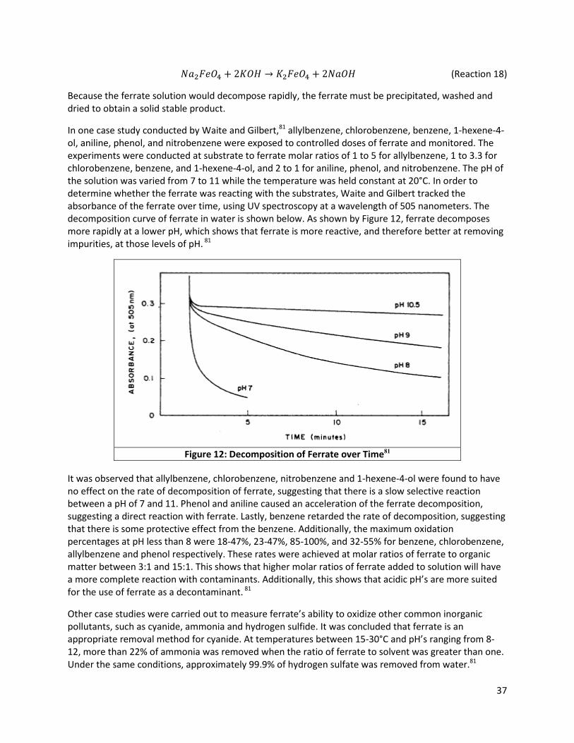
37

D ;�&< + 2�&% → � ;�&< + 2D&% (Reaction 18)

Because the ferrate solution would decompose rapidly, the ferrate must be precipitated, washed and

dried to obtain a solid stable product.

In one case study conducted by Waite and Gilbert,81 allylbenzene, chlorobenzene, benzene, 1-hexene-4-

ol, aniline, phenol, and nitrobenzene were exposed to controlled doses of ferrate and monitored. The

experiments were conducted at substrate to ferrate molar ratios of 1 to 5 for allylbenzene, 1 to 3.3 for

chlorobenzene, benzene, and 1-hexene-4-ol, and 2 to 1 for aniline, phenol, and nitrobenzene. The pH of

the solution was varied from 7 to 11 while the temperature was held constant at 20°C. In order to

determine whether the ferrate was reacting with the substrates, Waite and Gilbert tracked the

absorbance of the ferrate over time, using UV spectroscopy at a wavelength of 505 nanometers. The

decomposition curve of ferrate in water is shown below. As shown by Figure 12, ferrate decomposes

more rapidly at a lower pH, which shows that ferrate is more reactive, and therefore better at removing

impurities, at those levels of pH. 81

Figure 12: Decomposition of Ferrate over Time81

It was observed that allylbenzene, chlorobenzene, nitrobenzene and 1-hexene-4-ol were found to have

no effect on the rate of decomposition of ferrate, suggesting that there is a slow selective reaction

between a pH of 7 and 11. Phenol and aniline caused an acceleration of the ferrate decomposition,

suggesting a direct reaction with ferrate. Lastly, benzene retarded the rate of decomposition, suggesting

that there is some protective effect from the benzene. Additionally, the maximum oxidation

percentages at pH less than 8 were 18-47%, 23-47%, 85-100%, and 32-55% for benzene, chlorobenzene,

allylbenzene and phenol respectively. These rates were achieved at molar ratios of ferrate to organic

matter between 3:1 and 15:1. This shows that higher molar ratios of ferrate added to solution will have

a more complete reaction with contaminants. Additionally, this shows that acidic pH’s are more suited

for the use of ferrate as a decontaminant. 81

Other case studies were carried out to measure ferrate’s ability to oxidize other common inorganic

pollutants, such as cyanide, ammonia and hydrogen sulfide. It was concluded that ferrate is an

appropriate removal method for cyanide. At temperatures between 15-30°C and pH’s ranging from 8-

12, more than 22% of ammonia was removed when the ratio of ferrate to solvent was greater than one.

Under the same conditions, approximately 99.9% of hydrogen sulfate was removed from water.81

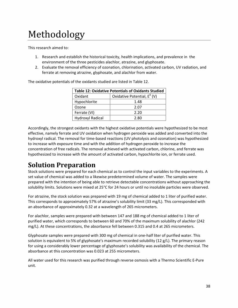
38

Methodology This research aimed to:

1. Research and establish the historical toxicity, health implications, and prevalence in the

environment of the three pesticides alachlor, atrazine, and glyphosate.

2. Evaluate the removal efficiency of ozonation, chlorination, activated carbon, UV radiation, and

ferrate at removing atrazine, glyphosate, and alachlor from water.

The oxidative potentials of the oxidants studied are listed in Table 12.

Table 12: Oxidative Potentials of Oxidants Studied

Oxidant Oxidative Potential, E0 (V)

Hypochlorite 1.48

Ozone 2.07

Ferrate (VI) 2.20

Hydroxyl Radical 2.80

Accordingly, the strongest oxidants with the highest oxidative potentials were hypothesized to be most

effective, namely ferrate and UV oxidation when hydrogen peroxide was added and converted into the

hydroxyl radical. The removal for time-based reactions (UV photolysis and ozonation) was hypothesized

to increase with exposure time and with the addition of hydrogen peroxide to increase the

concentration of free radicals. The removal achieved with activated carbon, chlorine, and ferrate was

hypothesized to increase with the amount of activated carbon, hypochlorite ion, or ferrate used.

Solution Preparation Stock solutions were prepared for each chemical as to control the input variables to the experiments. A

set value of chemical was added to a likewise predetermined volume of water. The samples were

prepared with the intention of being able to retrieve detectable concentrations without approaching the

solubility limits. Solutions were mixed at 25°C for 24 hours or until no insoluble particles were observed.

For atrazine, the stock solution was prepared with 19 mg of chemical added to 1 liter of purified water.

This corresponds to approximately 57% of atrazine’s solubility limit (33 mg/L). This corresponded with

an absorbance of approximately 0.32 at a wavelength of 265 micrometers.

For alachlor, samples were prepared with between 147 and 188 mg of chemical added to 1 liter of

purified water, which corresponds to between 60 and 70% of the maximum solubility of alachlor (242

mg/L). At these concentrations, the absorbance fell between 0.315 and 0.4 at 265 micrometers.

Glyphosate samples were prepared with 300 mg of chemical in one-half liter of purified water. This

solution is equivalent to 5% of glyphosate’s maximum recorded solubility (12 g/L). The primary reason

for using a considerably lower percentage of glyphosate’s solubility was availability of the chemical. The

absorbance at this concentration was 0.023 at 255 micrometers.

All water used for this research was purified through reverse osmosis with a Thermo Scientific E-Pure

unit.

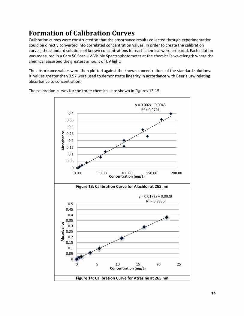
39

Formation of Calibration Curves Calibration curves were constructed so that the absorbance results collected through experimentation

could be directly converted into correlated concentration values. In order to create the calibration

curves, the standard solutions of known concentrations for each chemical were prepared. Each dilution

was measured in a Cary 50 Scan UV-Visible Spectrophotometer at the chemical’s wavelength where the

chemical absorbed the greatest amount of UV light.

The absorbance values were then plotted against the known concentrations of the standard solutions.

R2 values greater than 0.97 were used to demonstrate linearity in accordance with Beer’s Law relating

absorbance to concentration.

The calibration curves for the three chemicals are shown in Figures 13-15.

Figure 13: Calibration Curve for Alachlor at 265 nm

Figure 14: Calibration Curve for Atrazine at 265 nm

y = 0.002x - 0.0043

R² = 0.9791

0

0.05

0.1

0.15

0.2

0.25

0.3

0.35

0.4

0.00 50.00 100.00 150.00 200.00

Ab

sorb

an

ce

Concentration (mg/L)

y = 0.0172x + 0.0029

R² = 0.9996

0

0.05

0.1

0.15

0.2

0.25

0.3

0.35

0.4

0.45

0.5

0 5 10 15 20 25

Ab

sorb

an

ce

Concentration (mg/L)

40

Activated Carbon Adsorption

Two types of activated carbon were used to remove the pesticides

from water. The two types of activated carbon are powdered and

granular activated carbon. As the name suggests, the powdered

activated carbon (PAC) came in a powder while the granular activated

carbon (GAC) came in slightly larger particles. The same procedure

was used for both types of activated carbon to ensure consistency.

For each sample, a mass of activated carbon was added to 40-mL glass

vial. A volume of the aqueous pesticide solution was then added to

the vial. Vials were sealed and put into a rotator to mix for 24 hours.

The rotator rotated at a constant speed during this time. For all

samples, the 24-hour residence time remained constant while

amounts of pesticide and activated carbon varied.

The mass ratio of pesticide to activated carbon was varied in order to find the most effective ratio for

removal. Isotherms were plotted in which the equilibrium concentration was graphed versus the mass

of pesticide removed divided by the mass of activated carbon used. Depending on resulting data, the

mass ratio between pesticide and activated carbon was changed in order to get data points at the

appropriate range.

Once the vial was removed from the rotator, it was transferred to an Eppendorf Centrifuge 5804. Due

to the physical constraints of the glass vial, the centrifuge was set to spin the vials at 2600 rpm.

Depending on the type of activated carbon, the time in which the centrifuge would spin the sample

would vary from 15 to 45 minutes. After centrifugation, samples were removed and scanned in the UV

spectrophotometer to measure the absorbance level. The level was recorded and the resulting

concentration was plotted.

Figure 15: Calibration Curve for Glyphosate at 255 nm

Figure 16: Activated Carbon

y = 2E-05x + 0.0002

R² = 0.9905

0

0.002

0.004

0.006

0.008

0.01

0.012

0 100 200 300 400 500 600

Ab

sorb

an

ce

Concentration (mg/L)

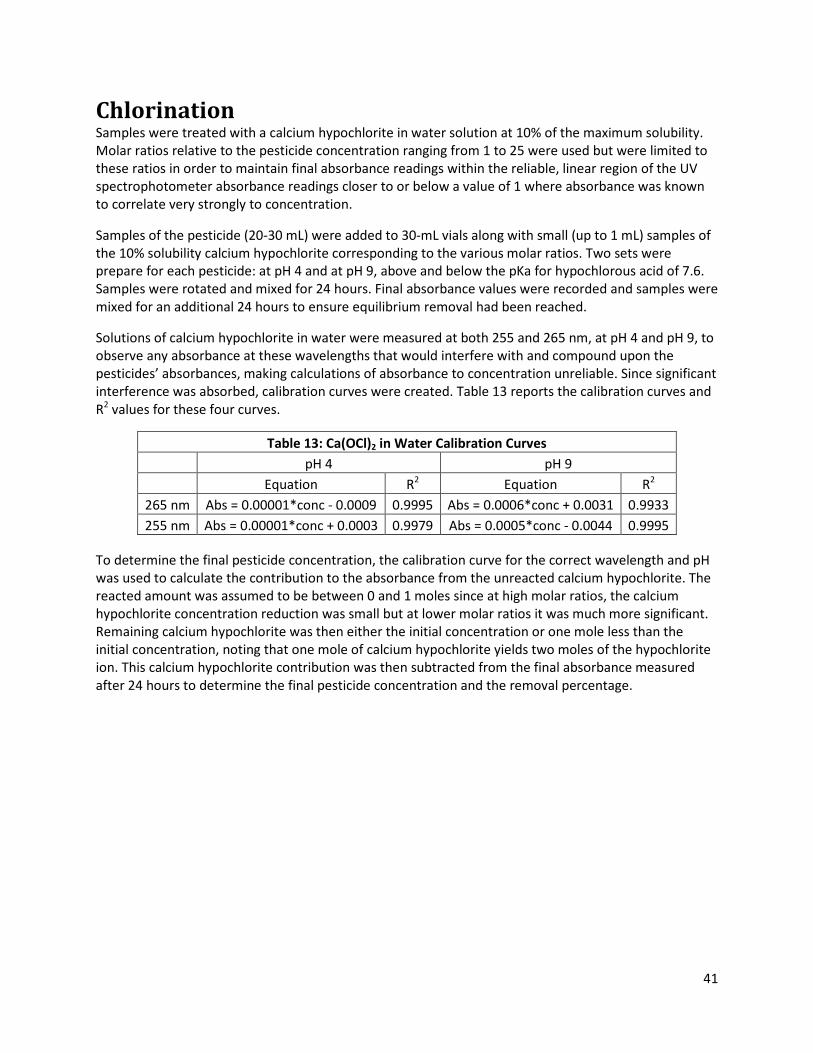
41

Chlorination Samples were treated with a calcium hypochlorite in water solution at 10% of the maximum solubility.

Molar ratios relative to the pesticide concentration ranging from 1 to 25 were used but were limited to

these ratios in order to maintain final absorbance readings within the reliable, linear region of the UV

spectrophotometer absorbance readings closer to or below a value of 1 where absorbance was known

to correlate very strongly to concentration.

Samples of the pesticide (20-30 mL) were added to 30-mL vials along with small (up to 1 mL) samples of

the 10% solubility calcium hypochlorite corresponding to the various molar ratios. Two sets were

prepare for each pesticide: at pH 4 and at pH 9, above and below the pKa for hypochlorous acid of 7.6.

Samples were rotated and mixed for 24 hours. Final absorbance values were recorded and samples were

mixed for an additional 24 hours to ensure equilibrium removal had been reached.

Solutions of calcium hypochlorite in water were measured at both 255 and 265 nm, at pH 4 and pH 9, to

observe any absorbance at these wavelengths that would interfere with and compound upon the

pesticides’ absorbances, making calculations of absorbance to concentration unreliable. Since significant

interference was absorbed, calibration curves were created. Table 13 reports the calibration curves and

R2 values for these four curves.

Table 13: Ca(OCl)2 in Water Calibration Curves

pH 4 pH 9

Equation R2 Equation R2

265 nm Abs = 0.00001*conc - 0.0009 0.9995 Abs = 0.0006*conc + 0.0031 0.9933

255 nm Abs = 0.00001*conc + 0.0003 0.9979 Abs = 0.0005*conc - 0.0044 0.9995

To determine the final pesticide concentration, the calibration curve for the correct wavelength and pH

was used to calculate the contribution to the absorbance from the unreacted calcium hypochlorite. The

reacted amount was assumed to be between 0 and 1 moles since at high molar ratios, the calcium

hypochlorite concentration reduction was small but at lower molar ratios it was much more significant.

Remaining calcium hypochlorite was then either the initial concentration or one mole less than the

initial concentration, noting that one mole of calcium hypochlorite yields two moles of the hypochlorite

ion. This calcium hypochlorite contribution was then subtracted from the final absorbance measured

after 24 hours to determine the final pesticide concentration and the removal percentage.

42

Ozonation

A tank containing oxygen was connected to an ozone generator and

pumped into the generator at a flow rate of 8 SCFH. The flow of

oxygen was acted upon by an electrical current to convert diatomic

oxygen into ozone. While the actual potential supplied by the unit

was unknown, the setting was kept at its maximum setting for the

duration of the experiment in order to maximize the amount of

ozone produced. The value of the applied potential was unknown

due to the limited information reported by the generator. No units

were given, only a numerical dial having no without a provided

correlation to the actual potential. The ozone gas and resulting free

radicals were then fed through a contactor into a flask containing the

solution, shown in Figure 17.

An Erlenmeyer flask was used to contain 75 mL of pesticide solution.

The ozone contactor was then placed into the flask and ozone

generator was started, feeding ozone gas into the solution. The flask

remained uncovered to allow the escape of waste gases. The contact

time for the ozone ranged from 5 to 90 minutes with absorption

readings taken every 5-15 minutes.

After each 5-15 minute interval, aqueous samples were extracted in order to measure the absorbance.

Before the sample could be measured however, the excess ozone in the solution needed to be

extracted. The half-life of ozone dissolved in water is about 30 minutes.54 In order to expedite this

process, two extraction methods were used. The two methods were an agitator and a sonification bath.

The agitator was a simple stir bar in the solution. The stir bar was set to an approximate speed of 350

rpm. The contact time for the agitator was in a ratio of 1:1 with how long the solution was treated with

ozone. The second extraction method used was a sonication bath. The bath was filled with purified

water just deep enough to cover the portion of the flask filled with the solution. The contact time for the

sonication bath was approximately 20 minutes regardless of the contact time with the ozone generator.

Because of the static residence time, the sonification bath was the primary means of extraction.

Figure 17: Ozonation Contactor

43

UV Photolysis

UV photolysis was used to reduce pesticide concentrations with

and without the addition of hydrogen peroxide. A low pressure

mercury vapor Pen-Ray 5.5 watt lamp (ACE No. 12132-08)

supplying UV light at 254 nm and a medium pressure UV lamp, the

Spectronics Corporation Spectroline 36-380 Long Wave Pencil

Lamp, supplying UV light at 365 nm were both used. Figure 18

shows a schematic of the lab scale reactor where a glass tube

holds an aqueous sample (6 mL) while UV light is applied for a

specified period of time. After this exposure time, the sample’s

absorbance was measured at the specified wavelength to

determine the final pesticide concentration as compared to the

initial concentration.

The exposure time was first set at 90 minutes to measure the

maximum removal when any subsequent UV exposure did not lead

to further concentration reduction. Both lamps were used at this

stage to determine which wavelength would be most effective for

each pesticide. The determinedly more effective lamp was used

for each respective pesticide for further tests. For all three

pesticides, the low-pressure lamp was more effective.

Trials at smaller time intervals were then conducted to observe the

rate of degradation under UV exposure. These were run at 5 minutes, 15 minutes, 30 minutes, and 60

minutes. Further treatment was added as necessary if the removal of the pesticide was less than 90%.

For all samples, the absorbance at the pesticide’s characteristic wavelength was recorded. Scans of

absorbance’s from 500-200 nm were run to observe the potential for byproducts of the oxidation

reactions that could have contributed to the absorbance and have been misrepresented in

concentration-based analyses.

Hydrogen Peroxide Addition Hydrogen peroxide was then added in molar ratios of 12.5:1, 25:1 50:1 and 100:1 relative to the amount

of pesticide. The higher ratios were expected to be more effective based on the literature.

After each ratio was allowed to react for 45-60 minutes, the most effective ratio was then rerun and

monitored in shorter time intervals to observe the changes in concentration with respect to time. The

absorbance was measured at all time intervals. Scans of the absorbance from 500-200 nm were run

when byproducts were anticipated based on the results of UV treatment without hydrogen peroxide. A

sample size of 6 mL and the low pressure lamp were used for all runs.

Figure 18: UV Treatment Set Up

44

Ferrate Oxidation

Potassium ferrate, shown in Figure 19, was

used in various molar ratios relative to the

pesticide used. Molar ratios of 1:1, 2:1, 4:1,

8:1 and 16:1 of potassium ferrate to

glyphosate in water were used, with respect

to the iron species that reacts (1 mole of iron

in 1 mole of potassium ferrate). Solid

potassium ferrate was added to 40-mL vials

with volumes of the pesticide between 20-30

mL. The pH was lowered to 3 with the

addition of 1 M HCl since the reaction

proceeds further under acidic conditions.

The vials were then capped and then rotated and agitated for 24 hours. Solids and suspected dissolved

solids were present at this point so the pH was then raised to 8 to minimize the solubility of ferric

hydroxide.86 Various methods of removal were then attempted, including centrifugation at 2600 RPM

for up to 2 hours, gravity filtration through 25 mm Whatman glass microfiber filters, and vacuum

filtration through 0.22 um Millipore Durapore (PVDF) filters. Final samples were measured in the UV

spectrophotometer at glyphosate’s characteristic wavelength and also scanned from wavelengths of

500-200 nm to observe any other wavelengths where the solution absorbed.

Figure 19: Potassium Ferrate Solid and in Aqueous

Pesticide Solution

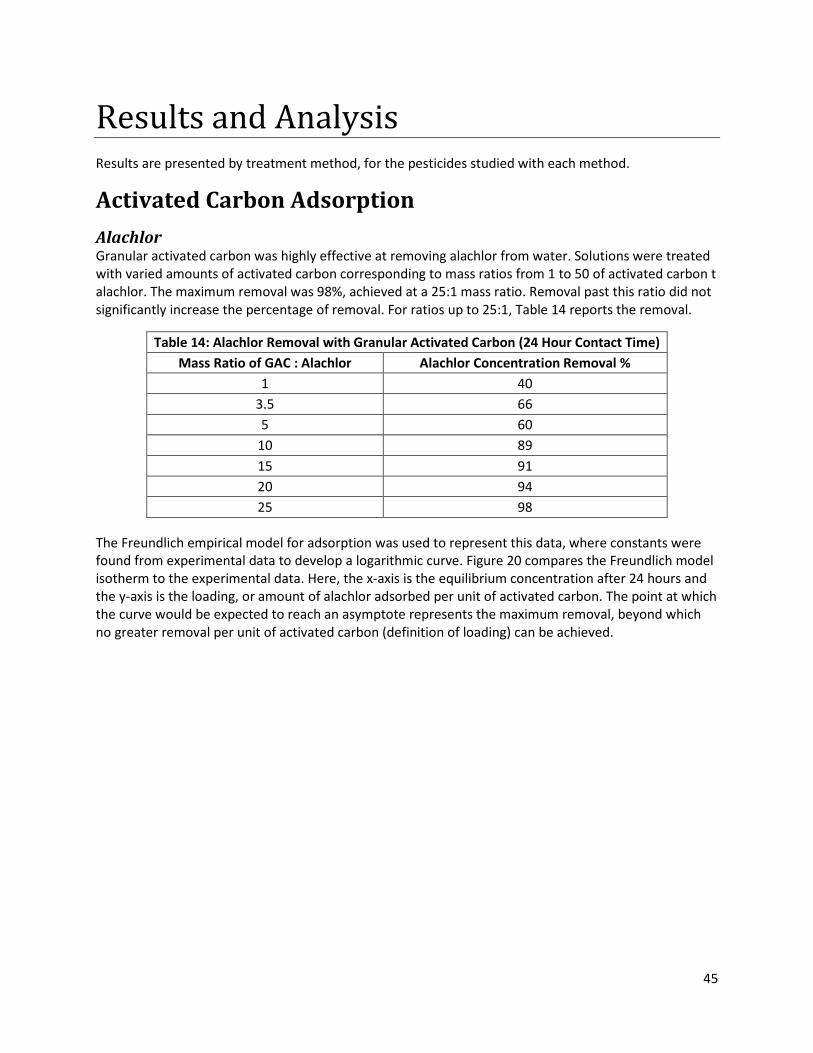
45

Results and Analysis Results are presented by treatment method, for the pesticides studied with each method.

Activated Carbon Adsorption

Alachlor Granular activated carbon was highly effective at removing alachlor from water. Solutions were treated

with varied amounts of activated carbon corresponding to mass ratios from 1 to 50 of activated carbon t

alachlor. The maximum removal was 98%, achieved at a 25:1 mass ratio. Removal past this ratio did not

significantly increase the percentage of removal. For ratios up to 25:1, Table 14 reports the removal.

Table 14: Alachlor Removal with Granular Activated Carbon (24 Hour Contact Time)

Mass Ratio of GAC : Alachlor Alachlor Concentration Removal %

1 40

3.5 66

5 60

10 89

15 91

20 94

25 98

The Freundlich empirical model for adsorption was used to represent this data, where constants were

found from experimental data to develop a logarithmic curve. Figure 20 compares the Freundlich model

isotherm to the experimental data. Here, the x-axis is the equilibrium concentration after 24 hours and

the y-axis is the loading, or amount of alachlor adsorbed per unit of activated carbon. The point at which

the curve would be expected to reach an asymptote represents the maximum removal, beyond which

no greater removal per unit of activated carbon (definition of loading) can be achieved.

46

Figure 20: Alachlor GAC Isotherm

Atrazine Activated carbon was highly effective in removing atrazine from water. Since the concentrations of

atrazine in solution were low and limited by the solubility of atrazine, greater masses of activated

carbon were required for accurate measurements. Therefore, mass ratios up to approximately 4,000:1

of activated carbon to pesticide were used. Table 15 reports the various ratios and their corresponding

removal rates. A 92% removal was achieved with a mass ratio of activated carbon to atrazine of 18:1.

Mass ratios greater than this did lead to slightly greater removal, but the much larger amounts of

activated carbon required indicate that a lower molar ratio would be more appropriate from a cost

analysis. A mass ratio between 18 and 117 should be investigated to determine the minimum mass ratio

required to increase removal up to 95%.

Table 15: Atrazine Removal with Granular Activated Carbon (24 Hour

Contact Time)

Mass Ratio of GAC : Atrazine Atrazine Concentration Removal %

3 21

7 53

18 92

117 96

2270 97

3422 97

Figure 21 shows the Freundlich isotherm for the atrazine experimental data. The data points

logarithmically ascend until a horizontal asymptote is reached at a loading of approximately 400.

0

20

40

60

80

100

120

140

160

0 20 40 60 80 100 120

Loa

din

g (

mg

/g)

Equilibrium Concentration (mg/L)

Experimental

Freundlich

47

Figure 21: Atrazine GAC Isotherm

Glyphosate Granular activated carbon displayed only a poor to moderate level of removal of glyphosate from water.

Solutions of glyphosate were treated with the activated carbon for 24 hours in mass ratios of activated

carbon to glyphosate ranging from 0.1:1 to 25:1. The solutions displayed unpredicted behavior, with

ratios above 15:1 displayed drastically decreased adsorption of chemical. The greatest removal was

approximately 51% at this 15:1 ratio. Table 16 shows the percent removal of glyphosate achieved at

corresponding mass ratios.

Table 16: Glyphosate Removal with Granular Activated Carbon (24 Hour Contact Time)

Mass Ratio of GAC : Glyphosate Glyphosate Concentration Removal %

0.1 3.7

0.5 4.7

1 3.8

5 15.7

10 45.4

15 50.7

Figure 22 shows the Freundlich isotherm alongside the experimental adsorption data.

0

20

40

60

80

100

120

140

160

180

200

0 5 10 15 20 25 30

Loa

din

g (

mg

/L)

Equilibrium Concentration (mg/L)

Experimental

Fruendlich

48

Figure 22: Glyphosate GAC Isotherm

Activated Carbon Adsorption Summary

Figure 23 shows Freundlich isotherms modeling the removal for all three pesticides using granular

activated carbon for the 24 hour equilibrium contact period. Points are experimental data and the

curves are Freundlich isotherms. The different slopes of the curves indicate that the amount of pesticide

that may be removed per unit of activated carbon, or the loading (y-axis), varies largely among the three

pesticides. Atrazine requires less activated carbon for its removal than alachlor or glyphosate. The

equilibrium concentrations remaining in solution differ largely as well but this is affected by the starting

concentrations in solution. Since solutions were prepared based on each pesticides’ individual solubility,

similarity over the x-axis is not expected. That is, glyphosate was roughly 30 times as concentrated as

atrazine.

0

10

20

30

40

50

60

70

80

90

100

0 100 200 300 400 500 600

Loa

din

g (

mg

/L)

Equilibrium Concentration (mg/L)

Experimental

Freundlich

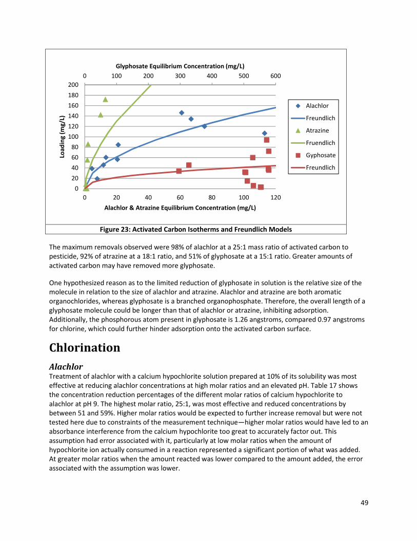
49

Figure 23: Activated Carbon Isotherms and Freundlich Models

The maximum removals observed were 98% of alachlor at a 25:1 mass ratio of activated carbon to

pesticide, 92% of atrazine at a 18:1 ratio, and 51% of glyphosate at a 15:1 ratio. Greater amounts of

activated carbon may have removed more glyphosate.

One hypothesized reason as to the limited reduction of glyphosate in solution is the relative size of the

molecule in relation to the size of alachlor and atrazine. Alachlor and atrazine are both aromatic

organochlorides, whereas glyphosate is a branched organophosphate. Therefore, the overall length of a

glyphosate molecule could be longer than that of alachlor or atrazine, inhibiting adsorption.

Additionally, the phosphorous atom present in glyphosate is 1.26 angstroms, compared 0.97 angstroms

for chlorine, which could further hinder adsorption onto the activated carbon surface.

Chlorination

Alachlor Treatment of alachlor with a calcium hypochlorite solution prepared at 10% of its solubility was most

effective at reducing alachlor concentrations at high molar ratios and an elevated pH. Table 17 shows

the concentration reduction percentages of the different molar ratios of calcium hypochlorite to

alachlor at pH 9. The highest molar ratio, 25:1, was most effective and reduced concentrations by

between 51 and 59%. Higher molar ratios would be expected to further increase removal but were not

tested here due to constraints of the measurement technique—higher molar ratios would have led to an

absorbance interference from the calcium hypochlorite too great to accurately factor out. This

assumption had error associated with it, particularly at low molar ratios when the amount of

hypochlorite ion actually consumed in a reaction represented a significant portion of what was added.

At greater molar ratios when the amount reacted was lower compared to the amount added, the error

associated with the assumption was lower.

0 100 200 300 400 500 600

0

20

40

60

80

100

120

140

160

180

200

0 20 40 60 80 100 120

Glyphosate Equilibrium Concentration (mg/L)Lo

ad

ing

(m

g/L

)

Alachlor & Atrazine Equilibrium Concentration (mg/L)

Alachlor

Freundlich

Atrazine

Fruendlich

Gyphosate

Freundlich

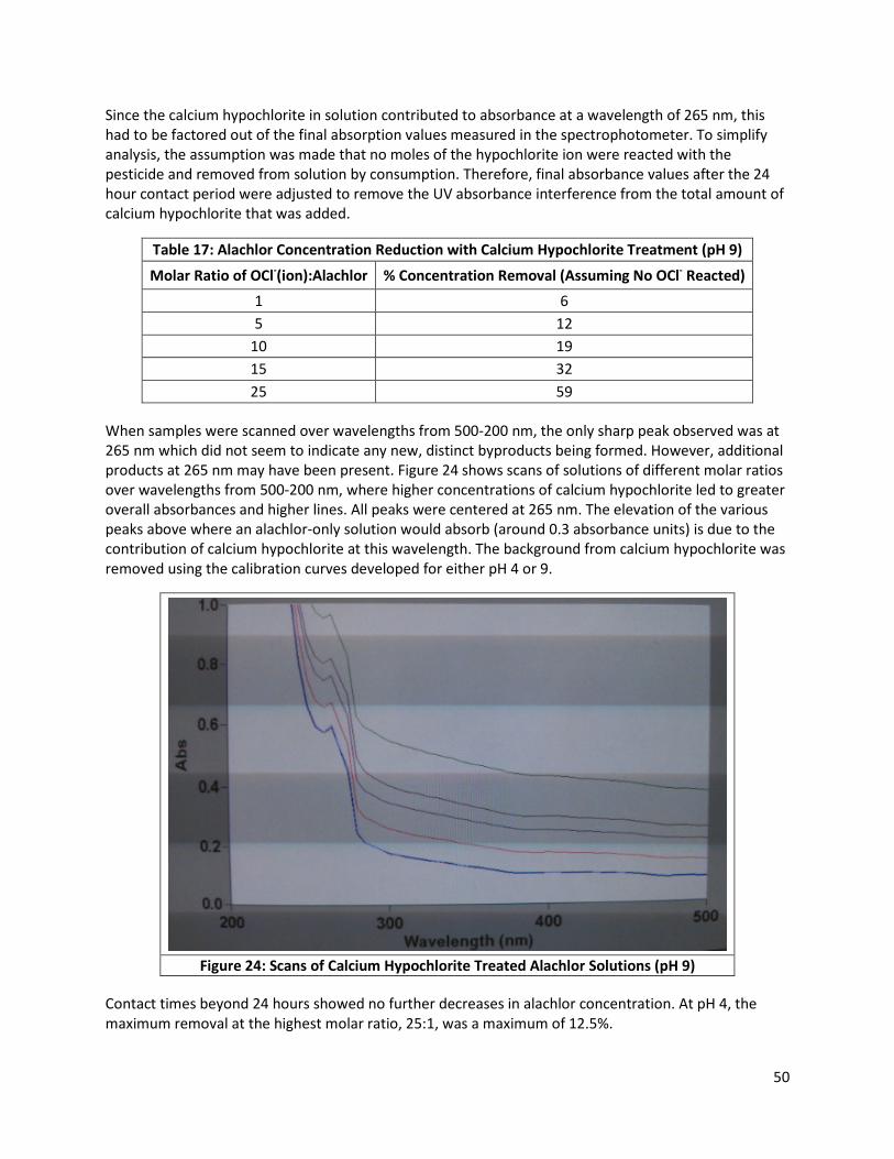
50

Since the calcium hypochlorite in solution contributed to absorbance at a wavelength of 265 nm, this

had to be factored out of the final absorption values measured in the spectrophotometer. To simplify

analysis, the assumption was made that no moles of the hypochlorite ion were reacted with the

pesticide and removed from solution by consumption. Therefore, final absorbance values after the 24

hour contact period were adjusted to remove the UV absorbance interference from the total amount of

calcium hypochlorite that was added.

Table 17: Alachlor Concentration Reduction with Calcium Hypochlorite Treatment (pH 9)

Molar Ratio of OCl-(ion):Alachlor % Concentration Removal (Assuming No OCl- Reacted)

1 6

5 12

10 19

15 32

25 59

When samples were scanned over wavelengths from 500-200 nm, the only sharp peak observed was at

265 nm which did not seem to indicate any new, distinct byproducts being formed. However, additional

products at 265 nm may have been present. Figure 24 shows scans of solutions of different molar ratios

over wavelengths from 500-200 nm, where higher concentrations of calcium hypochlorite led to greater

overall absorbances and higher lines. All peaks were centered at 265 nm. The elevation of the various

peaks above where an alachlor-only solution would absorb (around 0.3 absorbance units) is due to the

contribution of calcium hypochlorite at this wavelength. The background from calcium hypochlorite was

removed using the calibration curves developed for either pH 4 or 9.

Figure 24: Scans of Calcium Hypochlorite Treated Alachlor Solutions (pH 9)

Contact times beyond 24 hours showed no further decreases in alachlor concentration. At pH 4, the

maximum removal at the highest molar ratio, 25:1, was a maximum of 12.5%.

51

Atrazine Calcium hypochlorite was similarly more effective at removing atrazine at high molar ratios and an

elevated pH of 9. Table 18 reports the concentration reduction percentages for molar ratios from 1:1 up

to 25:1 at a pH of 9. The maximum removal at pH 4 was 3%. Scans of the treated solutions after 24

hours showed no new peak locations which would indicate byproducts.

Table 18: Atrazine Concentration Reduction with Calcium Hypochlorite Treatment (pH 9)

Molar Ratio of OCl-(ion):Alachlor % Concentration Removal (Assuming No OCl- Reacted)

1 3

5 9

10 12

15 14

25 11

Chlorination Summary Chlorine removal was expected to reach a maximum removal at some molar ratio of the hypochlorite

ion to the pesticide, and then remain near a constant removal percentage. This maximum removal was

observed for atrazine at a molar ratio of 15:1, at which 14% removal was achieved. The slight decrease

to 11% removal at a 25:1 molar ratio is attributed uncertainties in measurement techniques. Alachlor

removal would be also expected to reach a maximum removal, perhaps at molar ratio greater than 25:1,

beyond which the removal would not significantly increase or decrease. These percentages are based on

an assumption of 0 moles of hypochlorite being consumed in the reaction and therefore the background

from all added calcium hypochlorite being removed from the absorbance measured after treatment.

Analysis using this assumption is inaccurate at low molar ratios but becomes less inaccurate at higher

molar ratios. Therefore, this assumption of no hypochlorite reacted may be reliable for determination of

the maximum removals seen at high molar ratios.

Removal at pH 4 was much lower: 13% of alachlor and 3% of atrazine at the highest molar ratios used

(25:1). Since the pKa of hypochlorous acid is 7.6, the pH 4 samples featured the hypochlorous acid as the

dominant form of chlorine. The hypochlorite ion, dominant at pH levels greater than 7.6, was present in

greater amounts at pH 9 and is concluded to be a stronger oxidant than hypochlorous acid, contributing

to greater removal.

Ferrate The use of potassium ferrate to oxidize glyphosate yielded considerable degradation over the course of

a 24 hour contact time. This was determined qualitatively, based upon both the color of the solution

formed after the contact time and the amount of precipitate formed. However, soluble ferric

byproducts remained in solution despite attempts to filter or otherwise remove these solids. Therefore,

due to the high absorbance of these byproducts, quantitative measurements could not be appropriately

obtained from these samples to report the quantitative glyphosate removal. Multiple visual cues were

instead used to analyze the contaminant oxidation abilities of ferrate.

Firstly, the orange color that solutions developed over time was taken as an indication that reduction of

the iron was occurring. Potassium ferrate added to water initially had a purple color. At this point, iron

was in its +VI oxidation state. As reactions proceeded, the iron oxidized contaminants and was itself

reduced to its +III “ferric” oxidation state. This has a characteristic orange color. This therefore indicated

that the iron was reacting. The orange color of solutions can be seen in Figure 25, where samples’ molar

52

ratios of ferrate to glyphosate increased from 1:1 on the left-hand side up to 16:1 on the right-hand

side.

The depth of the orange color was further indicative of the reaction extent. Excess, unreacted iron in

solution is unstable and is known to be reduced to the more stable ferric form, which has a distinct

orange color. Therefore, the depth of the orange color in solution was used to infer the extent of

reaction—more of an orange color indicated a lower reaction extent since more iron remained

unreacted and was converted to ferric iron. Molar ratios leading to greater extents of reaction did not

produce as much ferric iron and had less of an orange color. Based on this color analysis, less-orange

solutions, or solutions with higher molar ratios, showed more complete reactions with glyphosate.

Solutions in which the reactions proceeded further produced more solid byproducts, which can also be

observed in Figure 25 where vials on the right-hand side (greater molar ratios, greater extents) have

greater solid content at the bottom. This corresponds to the hypothesis that the extent of the reaction

would be expected to increase with molar ratio since higher overall amounts of ferrate in solution

provided greater concentrations for the concentration-dependent reaction to occur.

Figure 25: Glyphosate Solutions after Ferrate Treatment, pH 3

These solutions could not be scanned in the UV spectrophotometer since soluble byproducts remained

in all solutions and contributed to absorbance values. In attempts to reduce this interference from the

byproducts, the experiment was repeated under acidic conditions to further the reaction at all molar

ratios. After a 24-hour reaction period, the solution’s pH was then raised to basic conditions (pH 8) to

minimize the solubility of the ferric compounds. The absorbance’s of the solutions were still above the

base absorbance of the glyphosate solution after being vacuum filtered and centrifuged at this elevated

pH. While the solutions visually appeared quite clear, as seen in Figure 26, it was concluded from the

elevated absorbance values was still a significant quantity of ferric component dissolved in the solution

that could not be removed sufficiently enough to obtain valid, quantitative data to describe the

glyphosate concentration reduction.

53

Figure 26: Glyphosate Solutions after Ferrate Treatment

and Solid Removal, pH 8

Although no valid quantitative data could be obtained from ferrate experiments, it was determined that

over the course of a 24 hour exposure time, potassium ferrate did eliminate a considerable percentage

of contaminant in solution. A considerable degree of oxidation could be anticipated based on the

oxidative potential of ferrate, 2.20. The solubility of byproducts must be evaluated and minimized more

thoroughly, if possible, to quantify final concentrations of an isolated pesticide compound.

Ozonation

Alachlor Ozone treatment of alachlor over time periods from 5 minutes up to 90 minutes did not successfully

reduce alachlor and alachlor byproduct concentrations. Instead, the absorbance at 265 nm rose steadily

until experiments were stopped at 90 minutes. The dose of ozone was not measurable but may be taken

as the maximum amount suppliable by the ozonator used.

As was observed with UV treatment, the peak at 265nm which indicates presence of alachlor decreased

rapidly while the total absorbance at 265 nm increased rapidly, and continued to increase with

continued exposure. Byproducts which did not show a peak on a scan of wavelengths 500-200 nm are

assumed to have contributed to the increase in absorbance. The increase in absorbance with ozone

contact time is shown in Figure 27. Exposure was limited to 90 minutes since greater contact time would

be impractical for treatment facilities and uneconomical. After 90 minutes, the absorbance had

increased by 49%. Again, for comparison, the untreated starting solution of alachlor (shown at 0 minutes

of contact time) began with an absorbance value of approximately 0.3.

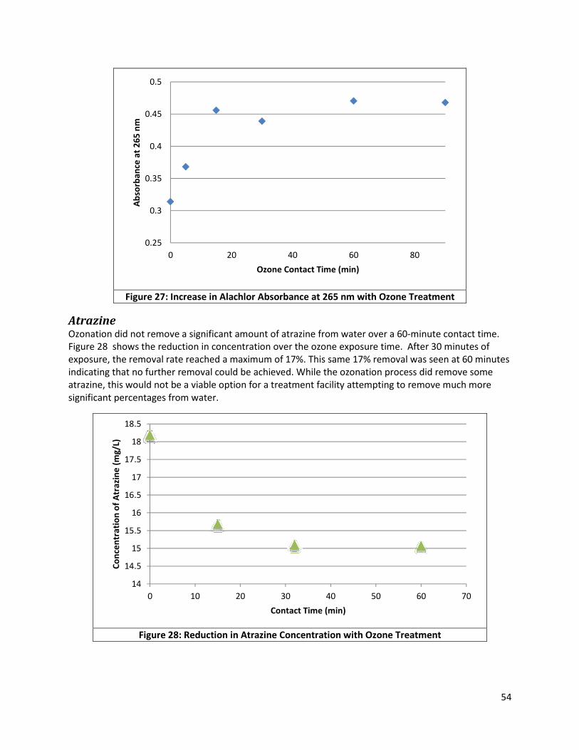
54

Figure 27: Increase in Alachlor Absorbance at 265 nm with Ozone Treatment

Atrazine Ozonation did not remove a significant amount of atrazine from water over a 60-minute contact time.

Figure 28 shows the reduction in concentration over the ozone exposure time. After 30 minutes of

exposure, the removal rate reached a maximum of 17%. This same 17% removal was seen at 60 minutes

indicating that no further removal could be achieved. While the ozonation process did remove some

atrazine, this would not be a viable option for a treatment facility attempting to remove much more

significant percentages from water.

Figure 28: Reduction in Atrazine Concentration with Ozone Treatment

0.25

0.3

0.35

0.4

0.45

0.5

0 20 40 60 80

Ab

sorb

an

ce a

t 2

65

nm

Ozone Contact Time (min)

14

14.5

15

15.5

16

16.5

17

17.5

18

18.5

0 10 20 30 40 50 60 70

Co

nce

ntr

ati

on

of

Atr

azi

ne

(m

g/L

)

Contact Time (min)

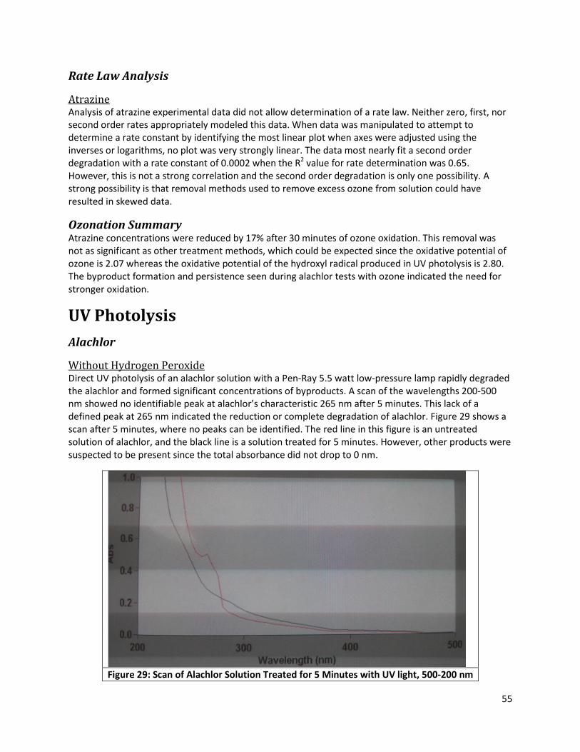
55

Rate Law Analysis

Atrazine Analysis of atrazine experimental data did not allow determination of a rate law. Neither zero, first, nor

second order rates appropriately modeled this data. When data was manipulated to attempt to

determine a rate constant by identifying the most linear plot when axes were adjusted using the

inverses or logarithms, no plot was very strongly linear. The data most nearly fit a second order

degradation with a rate constant of 0.0002 when the R2 value for rate determination was 0.65.

However, this is not a strong correlation and the second order degradation is only one possibility. A

strong possibility is that removal methods used to remove excess ozone from solution could have

resulted in skewed data.

Ozonation Summary Atrazine concentrations were reduced by 17% after 30 minutes of ozone oxidation. This removal was

not as significant as other treatment methods, which could be expected since the oxidative potential of

ozone is 2.07 whereas the oxidative potential of the hydroxyl radical produced in UV photolysis is 2.80.

The byproduct formation and persistence seen during alachlor tests with ozone indicated the need for

stronger oxidation.

UV Photolysis

Alachlor

Without Hydrogen Peroxide Direct UV photolysis of an alachlor solution with a Pen-Ray 5.5 watt low-pressure lamp rapidly degraded

the alachlor and formed significant concentrations of byproducts. A scan of the wavelengths 200-500

nm showed no identifiable peak at alachlor’s characteristic 265 nm after 5 minutes. This lack of a

defined peak at 265 nm indicated the reduction or complete degradation of alachlor. Figure 29 shows a

scan after 5 minutes, where no peaks can be identified. The red line in this figure is an untreated

solution of alachlor, and the black line is a solution treated for 5 minutes. However, other products were

suspected to be present since the total absorbance did not drop to 0 nm.

Figure 29: Scan of Alachlor Solution Treated for 5 Minutes with UV light, 500-200 nm

56

The total absorbance at 265 nm initially increased with time, reached a maximum absorbance at 90

minutes of UV exposure, and then began to decreased. The component which absorbed at 265 nm could

not be identified as either alachlor or a byproduct using only the spectrophotometer. It was concluded

that a large portion of the alachlor was degraded since no peak was seen on a 200-500 nm scan (Figure

29) but some amount of alachlor may have remained. No other clear peak was visible on the scan which

would have been specific to the byproduct(s) and could have helped identify their identities. However,

byproducts are believed to be formed, with the assumption that they may have absorbed UV light over a

range of wavelengths, lending themselves to no peak at a specific wavelength.

At 90 minutes, the maximum amount of these byproducts had been formed. The absorbance at 265 nm

reached 1.7, corresponding to a 5.4x increase from the solution’s starting absorbance. Scans of solutions

with longer contact times past 90 minutes showed subsequent decreases in the absorbance at 265 nm,

but still no formation of a second peak. Byproducts could not be identified but were observed to

decrease in concentration with time. Experiments were not extended to attempt to determine the

maximum reduction in absorbance beyond 2.5 hours, when the absorbance was still above 1.19 (4x the

initial absorbance). Figure 30 shows the increase, maximum, and decrease in the absorbance at 265 nm

with continued UV photolysis. This is presented in units of absorbance rather than concentration since

unidentifiable byproducts may have potentially contributed to this absorbance at 265 nm. UV photolysis

alone was unable to reduce alachlor/alachlor byproduct concentrations significantly in less than 90

minutes.

Figure 30: Increase in Alachlor Absorbance with UV Photolysis

With Hydrogen Peroxide

Advanced UV oxidation of alachlor with the addition of hydrogen peroxide showed more rapid and more

thorough reduction of the concentration of alachlor and/or alachlor byproducts. Of the 12.5:1, 25:1,

50:1, and 100:1 molar ratios of hydrogen peroxide to alachlor which were employed, the 25:1 molar

ratio was most successful at reducing the absorbance at 265 nm after 45 minutes, shown in Table 19.

This absorbance was still higher than the starting absorbance of alachlor alone, but longer residence

times were expected to reduce the absorbance further. Therefore, this 25:1 molar ratio was used over a

0.0

0.2

0.4

0.6

0.8

1.0

1.2

1.4

1.6

1.8

0 20 40 60 80 100 120 140

Ala

chlo

r A

bso

rba

nce

UV Contact Time (min)

57

longer time period to test the maximum alachlor removal over time. In Table 19, absorbance is again

used to report removal since byproducts were again concluded to be present.

Table 19: Evaluation of Various Molar Ratios of Hydrogen Peroxide : Alachlor for Use in UV Photolysis

Molar Ratio Absorbance at 265nm, 45 min

12.5 0.735

25 0.067

50 0.069

100 0.136

Scans over wavelengths of 500-200 nm for all UV and hydrogen peroxide-treated samples saw a lack of a

defined peak at 265 nm that would have indicated a high concentration of alachlor remaining. As was

seen without hydrogen peroxide use, no new peak was present that would indicate specific byproducts.

The 25:1 molar ratio of hydrogen peroxide to alachlor removed 88% of the species absorbing at 265 nm

after 60 minutes. After 90 minutes, this removal increased to a maximum of 95%. Table 20 reports the

percentages of absorbance reduction with increased exposure. Further exposure (up to 105) minutes

did not significant increase removal.

Table 20: Reduction in Alachlor Absorbance with UV + H2O2 (25:1 Molar Ratio)

Exposure Time (min) Reduction in Absorbance at 265 nm (%)

5 -312

15 -100

30 49

45 76

60 88

75 93

90 95

105 95

Figure 31 shows the same removal with time as Table 20. Though the identity and number of

byproduct(s) could not be determined, analysis using absorbance remains valid through use of Beer’s

Law linking absorbance to concentration. The calibration curve to quantitatively link absorbance to

concentration remains unknown. For comparison, the starting absorbance of the untreated alachlor

solution was approximately 0.3 (shown at time zero).

58

Figure 31: Degradation of Alachlor with UV + H2O2 (25:1 Molar Ratio)

Kinetics Analysis

Rate analysis was performed to observe the degradation kinetics for UV treatment using hydrogen

peroxide. Since no appreciable degradation was seen without hydrogen peroxide addition, no kinetic

analysis was appropriate without hydrogen peroxide addition. For rate law determination,

concentration units were used although byproducts were certainly observed. The concentration was

calculated as if all absorbance was due to the alachlor base compound though this was known to be

inaccurate since no increase in alachlor concentration was possible. Because of this spike in

concentration that was attributed to byproduct formation, the rate law for the overall degradation that

was observed could be developed in two ways: the rate pertaining to the entire process, including the

rapid concentration increase, and that of the rate just concerning the degradation that followed the

rapid concentration increase.

Manipulation of the axes to determine the rate order led to a first order rate determination. When the

initial spike in concentration was included, the rate constant in this case was determined to be 0.0412

min-1. Without this initial spike in concentration, the rate constant in this case was determined to be

0.0457 min-1. The rates would not vary too greatly by using either analysis method, but here the rate

constant was selected so as to include the initial spike in concentration since it seemed to more

accurately describe the behavior observed. The rate law was then:

−EFGFHIGJK � 0.0457 ∗ �FGFHIGJK (Reaction 19)

Figure 32 shows the degradation of alachlor over time (in concentration units) along with the

degradation predicted by the rate law that was developed.

0

0.2

0.4

0.6

0.8

1

1.2

1.4

0 20 40 60 80 100

Ab

sorb

an

ce a

t 2

65

nm

UV Contact Time (min)

59

Figure 32: First Order Degradation of Alachlor with UV + H2O2 (25:1 Molar Ratio)

Atrazine

Without Hydrogen Peroxide The low-pressure UV lamp was used to treat atrazine solutions for 90 minutes. The overall removal

achieved was 87% in 75 minutes. Removal at 90 minutes was not significantly increased. Figure 33

shows the degradation of atrazine over time.

Figure 33: Degradation of Atrazine with UV Photolysis

0

100

200

300

400

500

600

700

0 20 40 60 80 100 120

Ala

chlo

r C

on

cen

tra

tio

n (

mg

/L)

Contact Time (min)

Alachlor

r=-0.0412*Ca

0

2

4

6

8

10

12

14

16

18

20

0 20 40 60 80 100

Co

nce

ntr

ati

on

of

Atr

azi

ne

(m

g/L

)

Time (min)

60

With Hydrogen Peroxide

Hydrogen peroxide was then added to the atrazine solution at a molar ratio of 100:1. Again, the low

solubility of atrazine led to this high ratio since lower ratios would have resulted in nearly negligible

amounts of hydrogen peroxide added. A 63% increase in concentration was observed during the first 15

minutes of exposure. The solution was hypothesized to have degraded into atrazine’s byproducts due to

the hydrogen peroxide addition. Figure 34 shows the atrazine degradation with time. After 120 minutes

the removal reached a maximum of 92%.

Figure 34: Degradation of Atrazine with UV + H2O2 (100:1 Molar Ratio)

Kinetics Analysis It was determined through graphical analysis that the degradation of atrazine with UV photolysis first

order reaction with a rate constant of 0.0245 min-1. The rate law, shown in Figure 35 with experimental

data, was then:

−EFLKFMN� � 0.0245 ∗ �FLKFMN� (Reaction 20)

0

5

10

15

20

25

30

35

40

0 20 40 60 80 100 120

Co

nce

ntr

ati

on

of

Atr

azi

ne

(m

g/L

)

Time (min)

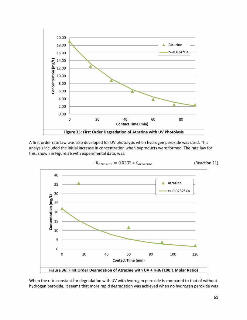
61

Figure 35: First Order Degradation of Atrazine with UV Photolysis

A first order rate law was also developed for UV photolysis when hydrogen peroxide was used. This

analysis included the initial increase in concentration when byproducts were formed. The rate law for

this, shown in Figure 36 with experimental data, was:

−EFLKFMN� � 0.0232 ∗ �FLKFMN� (Reaction 21)

Figure 36: First Order Degradation of Atrazine with UV + H202 (100:1 Molar Ratio)

When the rate constant for degradation with UV with hydrogen peroxide is compared to that of without

hydrogen peroxide, it seems that more rapid degradation was achieved when no hydrogen peroxide was

0.00

2.00

4.00

6.00

8.00

10.00

12.00

14.00

16.00

18.00

20.00

0 20 40 60 80

Co

nce

ntr

ati

on

(m

g/L

)

Contact Time (min)

Atrazine

r=-0.024*Ca

0

5

10

15

20

25

30

35

40

0 20 40 60 80 100 120

Co

nce

ntr

ati

on

(m

g/L

)

Contact Time (min)

Atrazine

r=-0.0232*Ca

62

added. The rate constant is greater when no hydrogen peroxide was added. This is because the spike in

concentration when byproducts were formed was included in the analysis when hydrogen peroxide was

added. No spike was seen without hydrogen peroxide, but perhaps at shorter time intervals a similar

spike would have been observed. Or, byproducts may have followed a different degradation pathway

involving byproducts that did not absorb as much UV light (as measured in the UV spectrophotometer)

when a greater concentration of hydroxyl radicals were present. The overall removal when contact

times reached 90 minutes became very similar.

Glyphosate

Without Hydrogen Peroxide Direct UV photolysis of a glyphosate solution under a low-pressure lamp showed significant reactions

occurring over a relatively short period of time. However, due to the significant amount of byproducts

produced by the degradation of glyphosate, absorbance was seen to rise steadily with time. While the

absorbance of alachlor and atrazine ultimately decreased over the course of the UV exposure, the

byproducts formed by glyphosate were slow to degrade with the UV exposure. The absorbance level

ultimately leveled off after two hours, at which point it could be concluded that the glyphosate had

ceased reacting, but did not decrease after this time period. When scanned from 200-500 nm, no visible

peaks were observed at 255 nm, which is glyphosate’s absorption wavelength. This observation led to

the conclusion that after two hours of UV exposure, most of the measurable glyphosate had been

reacted out of solution. No other peaks were visible on the scan to denote the byproducts’ identities.

However, the overall increase in absorbance at 255 nm does lend itself to byproducts, as there were no

other components within the solution that could react with the free radicals produced by UV photolysis.

Byproducts that formed may not have been measurable by the spectrophotometer.

At the 120 minute point, the absorbance of the solution had reached 0.085, almost seven times greater

than its initial absorbance. Figure 37 shows the increase of absorption at 255 nm with respect to UV

contact time. The graph is shown in terms of absorbance rather than concentration as the presence of

byproducts makes the conversion between absorbance and concentration impossible.

Figure 37: Increase in Glyphosate Absorbance with UV Photolysis

0

0.01

0.02

0.03

0.04

0.05

0.06

0.07

0.08

0.09

0 20 40 60 80 100 120 140 160

Ab

sorb

an

ce a

t 2

55

nm

Time (min)

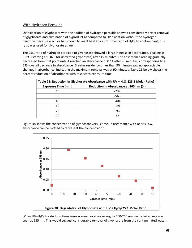
63

With Hydrogen Peroxide

UV oxidation of glyphosate with the addition of hydrogen peroxide showed considerably better removal

of glyphosate and elimination of byproduct as compared to UV oxidation without the hydrogen

peroxide. Because alachlor had shown to react best at a 25:1 molar ratio of H2O2 to contaminant, this

ratio was used for glyphosate as well.

The 25:1 ratio of hydrogen peroxide to glyphosate showed a large increase in absorbance, peaking at

0.193 (starting at 0.023 for untreated glyphosate) after 15 minutes. The absorbance reading gradually

decreased from that point until it reached an absorbance of 0.11 after 90 minutes, corresponding to a

52% overall decrease in absorbance. Greater residence times than 90 minutes saw no appreciable

changes in absorbance, indicating the maximum removal was at 90 minutes. Table 21 below shows the

percent reduction of absorbance with respect to exposure time.

Table 21: Reduction in Glyphosate Absorbance with UV + H2O2 (25:1 Molar Ratio)

Exposure Time (min) Reduction in Absorbance at 265 nm (%)

15 -739

30 -565

45 -404

60 -191

75 -96

90 52

Figure 38 shows the concentration of glyphosate versus time. In accordance with Beer’s Law,

absorbance can be plotted to represent the concentration.

Figure 38: Degradation of Glyphosate with UV + H2O2 (25:1 Molar Ratio)

When UV+H2O2 treated solutions were scanned over wavelengths 500-200 nm, no definite peak was

seen at 255 nm. This would suggest considerable removal of glyphosate from the contaminated water.

0.00

0.05

0.10

0.15

0.20

0.25

0 10 20 30 40 50 60 70 80 90

Ab

sorb

an

ce a

t 2

55

nm

Contact Time (min)

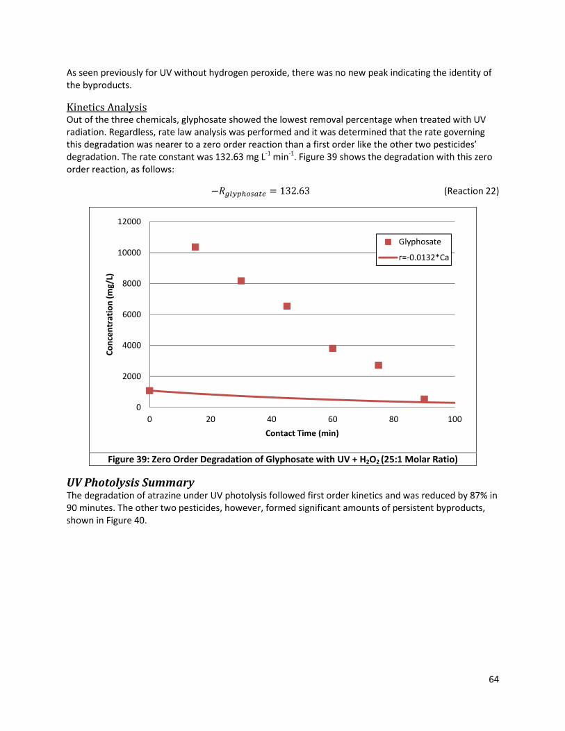
64

As seen previously for UV without hydrogen peroxide, there was no new peak indicating the identity of

the byproducts.

Kinetics Analysis Out of the three chemicals, glyphosate showed the lowest removal percentage when treated with UV

radiation. Regardless, rate law analysis was performed and it was determined that the rate governing

this degradation was nearer to a zero order reaction than a first order like the other two pesticides’

degradation. The rate constant was 132.63 mg L-1 min-1. Figure 39 shows the degradation with this zero

order reaction, as follows:

−EOGPQIJRFL� � 132.63 (Reaction 22)

Figure 39: Zero Order Degradation of Glyphosate with UV + H2O2 (25:1 Molar Ratio)

UV Photolysis Summary The degradation of atrazine under UV photolysis followed first order kinetics and was reduced by 87% in

90 minutes. The other two pesticides, however, formed significant amounts of persistent byproducts,

shown in Figure 40.

0

2000

4000

6000

8000

10000

12000

0 20 40 60 80 100

Co

nce

ntr

ati

on

(m

g/L

)

Contact Time (min)

Glyphosate

r=-0.0132*Ca

65

Figure 40: Alachlor and Glyphosate Byproduct Formation with UV photolysis

Stronger oxidation with hydrogen peroxide removed 95% of alachlor, 83% of atrazine, and 50% of

glyphosate in 90 minutes. The most effective molar ratios of hydrogen peroxide to pesticide were used.

The removal of atrazine slightly decreased with this addition of hydrogen peroxide, but this difference is

concluded to be due to errors associated with measurement of concentrations since atrazine

concentrations started lower than the other two pesticides. The removal of the other two pesticides

increased with the addition of hydrogen peroxide. This is because the hydroxyl radical, the oxidant that

is generated from water with UV exposure, is generated in greater concentrations when hydrogen

peroxide is added.

Removal of alachlor and atrazine with hydrogen peroxide followed first order kinetics. The experimental

data points as well as the curves showing degradation according to the generated rate laws are shown in

Figure 41.

0

0.01

0.02

0.03

0.04

0.05

0.06

0.07

0.08

0.09

0

0.2

0.4

0.6

0.8

1

1.2

1.4

1.6

1.8

0 20 40 60 80 100 120 140

Gly

ph

osa

te A

bso

rba

nce

Ala

chlo

r A

bso

rba

nce

Contact Time (min)

Alachlor

Glyphosate

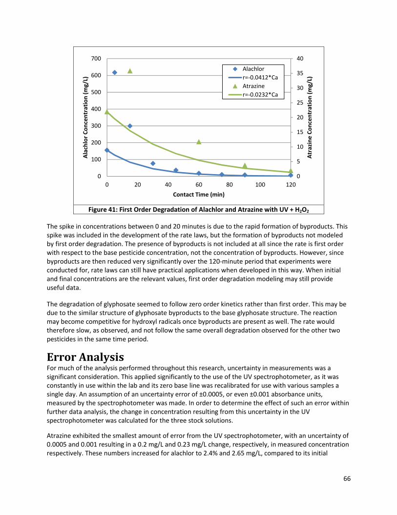
66

Figure 41: First Order Degradation of Alachlor and Atrazine with UV + H2O2

The spike in concentrations between 0 and 20 minutes is due to the rapid formation of byproducts. This

spike was included in the development of the rate laws, but the formation of byproducts not modeled

by first order degradation. The presence of byproducts is not included at all since the rate is first order

with respect to the base pesticide concentration, not the concentration of byproducts. However, since

byproducts are then reduced very significantly over the 120-minute period that experiments were

conducted for, rate laws can still have practical applications when developed in this way. When initial

and final concentrations are the relevant values, first order degradation modeling may still provide

useful data.

The degradation of glyphosate seemed to follow zero order kinetics rather than first order. This may be

due to the similar structure of glyphosate byproducts to the base glyphosate structure. The reaction

may become competitive for hydroxyl radicals once byproducts are present as well. The rate would

therefore slow, as observed, and not follow the same overall degradation observed for the other two

pesticides in the same time period.

Error Analysis For much of the analysis performed throughout this research, uncertainty in measurements was a

significant consideration. This applied significantly to the use of the UV spectrophotometer, as it was

constantly in use within the lab and its zero base line was recalibrated for use with various samples a

single day. An assumption of an uncertainty error of ±0.0005, or even ±0.001 absorbance units,

measured by the spectrophotometer was made. In order to determine the effect of such an error within

further data analysis, the change in concentration resulting from this uncertainty in the UV

spectrophotometer was calculated for the three stock solutions.

Atrazine exhibited the smallest amount of error from the UV spectrophotometer, with an uncertainty of

0.0005 and 0.001 resulting in a 0.2 mg/L and 0.23 mg/L change, respectively, in measured concentration

respectively. These numbers increased for alachlor to 2.4% and 2.65 mg/L, compared to its initial

0

5

10

15

20

25

30

35

40

0

100

200

300

400

500

600

700

0 20 40 60 80 100 120

Atr

azi

ne

Co

nce

ntr

ati

on

(m

g/L

)

Ala

chlo

r C

on

cen

tra

tio

n (

mg

/L)

Contact Time (min)

Alachlor

r=-0.0412*Ca

Atrazine

r=-0.0232*Ca

67

concentration of 160 mg/L. Glyphosate showed the most noticeable changes, showing a 35 mg/L and 60

mg/L uncertainty with respect to its initial concentration of 600 mg/L.

An additional source of error that was considered during experimentation was the measurement of

solids for various mass and molar ratios used throughout research. For solid compounds such as

activated carbon and potassium ferrate, there was uncertainty in the readouts of the scales used to

mass samples to the thousands decimal. Additionally, the varying size of particles of activated carbon

made maintaining precise ratios difficult since the addition of a single granule of activated carbon in

some cases pushed the mass ratio slightly beyond what was desired. However, the effect of such an

error would be considered to be minimal.

Liquid compounds such as hydrogen peroxide and calcium hypochlorite solution also added sources of

error throughout experimentation. The use of micropipettes in conjunction with the use of minute

measurements of these liquids meant that any deviation from the desired volume could be significant.

For example, a measurement of 10 microliters off by 1 microliter led to a 10% error. In this case, the

source of the error would come from the precision and accuracy of a given micropipette or graduated

cylinder, as well as human error associated with pipetting and transferring fluids.

The contact time used for time-based treatments (UV photolysis and ozonation) may have deviated

slightly from the reported times. This deviation, likely a maximum of 2-3 minutes, would not have led to

a very significant alteration in the degradation behavior since most degradation was significant over 30-

90 minute time periods. Comparatively, the reaction occurring in a 2-3 minute time period would not

have a significant impact. For activated carbon, chlorine, and ferrate samples run for 24 hours,

equilibrium concentrations were reached (verified by measurements after 48 hours) so no error

associated with prolonged exposure were expected.

Since applied ozone concentrations could not be measured with the equipment and meters in the

laboratory, a great deal of uncertainty is associated with ozone treatment. However, experiments were

still conducted with the acceptance that quantitative values could not be obtained.

Byproduct formation also contributed to errors in our analysis. Since identities of byproducts could not

be determined using the UV spectrophotometer, concentrations of byproducts could not be

determined. No calibration curve correlating the absorbance to concentration could be produced.

Furthermore, the distinction between base pesticides and byproducts could not always be made since in

all cases, no secondary peaks were observed when samples were scanned from 500-200 nm. Byproducts

and base compounds were therefore analyzed together. When determining rate laws, concentration

units were used, with the acknowledgement that this concentration would be in terms of the base

pesticide concentrations—though byproducts were in fact present. This analysis is still valuable for

determination of contact time required to reduce concentrations to a significant level.

68

Conclusions and Recommendations The most effective treatment methods in terms of maximum possible removal were granular activated

carbon and advanced UV oxidation with hydrogen peroxide. The superiority of these two treatment

methods was observed for both alachlor and atrazine. Glyphosate was treated only with these two

methods and its removal therefore cannot be compared among other treatment methods.

A 25:1 mass ratio of activated carbon to alachlor was most effective at reducing concentrations for a 24-

hour contact time—a 98% reduction. An 18:1 mass ratio to atrazine effectively removed 92%. A 15:1

mass ratio to glyphosate effectively removed 51%.

A 25:1 molar ratio of hydrogen peroxide to alachlor was most effective at reducing the absorbance at

265 nm for a 90-minute residence time—a 95% reduction. First order kinetics were used to model this

removal. A 100:1 molar ratio of hydrogen peroxide to atrazine reduced the concentration for a 90-

minutes residence time by 83%. First order kinetics were again observed. A 25:1 molar ratio of hydrogen

peroxide to glyphosate reduced the concentration for a 90-minute residence time by 50%. This removal

did not follow first order and was instead concluded to be a competitive reaction for hydroxyl radicals

between glyphosate and its byproducts.

Calcium hypochlorite at the highest molar ratio removed only 59% of alachlor and 14% of atrazine at an

elevated pH. Significant amounts of byproducts were formed during UV, UV+H2O2, and ozone treatment.

Only UV+H2O2 was successful at reducing concentrations of these byproducts in a reasonable time

period (90 minutes). The identities of these byproducts could not be determined, and they did not show

a defined peak at any wavelength but were observed to absorb UV light over a range of wavelengths.

One recommendation made for future research includes the identification of these byproducts using a

mass spectrophotometer and gas chromatograph. These byproducts can be monitored over time to

observe degradation kinetics rather than grouping all degradation into first order kinetics with respect

to the base pesticide concentration.

The oxidative potentials of hypochlorite and of ozone, respectively, are 1.48 and 2.07. When these

potentials are compared to that of the hydroxyl radical, 2.80, the successful removal using UV photolysis

with added hydrogen peroxide was to be expected. The hydroxyl radical is the strongest oxidant and

was therefore the most successful at oxidizing pesticides.

Since the oxidative potential of ferrate is 2.20, the second highest of treatments used here, a method to

determine the quantitative pesticide concentration reduction with ferrate is recommended. This could

involve filtration through membranes with tighter pores or different surface chemistries. Another

method might involve determination of all reactions occurring, baking of products to determine the

amounts of solids, and analysis of the stoichiometry involved to isolate the amount of pesticide

remaining in solution as compared to the other solids formed during the reaction. The removal may be

determined in that matter.

Other recommendations include either increasing the concentration of ozone applied during ozonation

or adding hydrogen peroxide. Both would increase the amount of oxidants in solution and therefore

increase removal.

69

References (1) International Code of Conduct on the Distribution and Use of Pesticides. United Nations, Food

and Agricultural Organization: 2002, Rome.

(2) Raven, P. H.; Berg, L. R.; Hassenzahl, D. M. Environment, 6th ed.; John Wiley & Sons, Inc:

Hoboken, NJ, 2008.

(3) Gold, L. S.; Slone, T. H., Ames; B. N.; Manley, N. B. Immunotoxicity of Pesticides. In Handbook

of Pesticide Toxicology; Krieger, R., Ed.; Academic Press: San Diego, 2001; p 769-778

(4) United States Environmental Protection Agency. Types of Pesticides.

http://www.epa.gov/opp00001/about/types.htm (accessed Nov 10, 2011).

(5) Fishel, F. M. Pesticide Toxicity Profile: Carbamate Pesticides. University of Florida, Institute of

Food and Agricultural Services (IFAS) Extension.

(6) United States Environmental Protection Agency. Pesticides. http://www.epa.gov/osw/hazard/

wastetypes/universal/pesticides.htm (accessed Nov 10, 2011).

(7) Extension Toxicology Network. Glyphosate. http://pmep.cce.cornell.edu/profiles/extoxnet/

dienochlor-glyphosate/glyphosate-ext.html (accessed 23 Nov 2012)

(8) Fishel, F. M. Evaluation of Pesticides for Carcinogenic Potential. University of Florida, Institute

of Food and Agricultural Services (IFAS) Extension: 2004.

(9) Davis, M. L.; Masten, S. J. Principles of Environmental Engineering and Science. McGraw-Hill:

New York, 2004.

(10) United States Environmental Protection Agency. Summary of the Clean Water Act.

http://www.epa.gov/lawsregs/laws/cwa.html (accessed Nov 25, 2011).

(11) Unites States Environmental Protection Agency. Safe Drinking Water Act.

http://water.epa.gov/lawsregs/rulesregs/sdwa/ (accessed Nov 25, 2011).

(12) United States Environmental Protection Agency. National Primary Drinking Water Regulations.

http://water.epa.gov/drink/contaminants/index.cfm (accessed Nov 25, 2011).

(13) Nesheim, O. N., Fishel, F. M., & Mossler, M. Toxicity of Pesticides. University of Florida,

Institute of Food and Agricultural Services (IFAS) Extension: 2009.

(14) Nation Research Council. Pesticides in the Diets of Infants and Children. National Academy

Press: Washington, DC, 1993.

(15) SCI. Proposals to restrict the use of pesticides in the European Union.

http://www.soci.org/News/BioResources-pesticide-regs (accessed November 25, 2011)

(16) Which Pesticides are Banned in Europe, Food & Fairness Briefing No. 1: 2008.

(17) European Commission. Health and Consumers. http://ec.europa.eu/food/plant/protection/

pesticides/index_en.htm (Accessed January 23, 2012)

(18) Hock, W. K., & Lorenz, E. S. Toxicity of Pesticides. Pennsylvania State University, College of

Agricultural Sciences: 2006.

(19) United States Environmental Protection Agency. Persistent Bioaccumulative and Toxic (PBT)

Chemical Program. http://www.epa.gov/pbt/pubs/execsumm.htm (accessed Jan 20, 2012).

(20) United States Environmental Protection Agency. National Action Plan for the Level 1

Pesticides. http://www.epa.gov/pbt/pubs/pestaction.htm#2.0 (accessed Dec 15, 2011).

(21) University of California - Berkeley. Pesticide Atrazine Can Turn Male Frogs into

Females. ScienceDaily. Mar 2010, http://www.sciencedaily.com/releases/2010/

03/100301151927.htm

(22) Garry, V. F. Pesticides and Children. Toxicology and Applied Pharmacology. 2004, 198, 152-

163.

70

(23) Fishel, F. Pesticides and the Environment. University of Missouri Extension, Department of

Agronomy: 2005.

(24) British Columbia Ministry of Agriculture. Environmental Fate.

http://www.agf.gov.bc.ca/pesticides/c_2.htm#1b (accessed March 23, 2012).

(25) Zbytniewski, R.; Buszewski, B. Sorption of Pesticides in Soil and Compost. Polish Journal of

Environmental Studies. 2002, 11, 179-184.

(26) Huggenberger, F., Letey, J. J.; Farmer, W. J. Adsorption and Mobility of Pesticides in Soil.

California Agriculture. 1973, 8-10.

(27) World Health Organization. WHO/FAO Data Sheet on Pesticides, No. 86 Alachlor,

WHO/PCS/DS/96.86 http://www.inchem.org/documents/pds/pds/pest86_e.htm (accessed

Dec 1, 2011).

(28) United States Environmental Protection Agency. R.E.D. Facts: Alachlor.

http://www.epa.gov/oppsrrd1/REDs/factsheets/0063fact.pdf (accessed Nov 5, 2011).

(29) Ahrens, W. H.; Hatzios, K. K.; Edwards, M. T. Herbicide Handbook. Herbicide Handbook

Committee. Weed Science Society of America: 1974.

(30) United States Environmental Protection Agency. Basic Information about Alachlor in Drinking

Water. http://water.epa.gov/drink/contaminants/basicinformation/alachlor.cfm (accessed

Nov 4, 2011).

(31) Rotterdam Convention on the Prior Informed Consent Procedure for Certain Hazardous

Chemicals and Pesticides in International Trade. Decision Guidance Document.

http://www.pic.int/Portals/5/DGDs/DGD_Alachlor_EN.pdf (accessed Mar 20, 2012).

(32) California Department of Pesticide Regulation. Wales, P. Use Information and Air Monitoring

Recommendation for the Pesticide Active Ingredient Alachlor; Sacramento, CA, 1997.

(33) Pothuluri, J.V., Moorman, T.B., Obenhuber, D.C., Wauchope, R.D. Aerobic and Anaerobic

Degradation of Alachlor in Samples from a Surface-to-Ground Water Profile. J. Environ. Qual.

1990, 19, 525–530.

(34) Chirnside, A. E. M.; Ritter, W. F.; Radosevich, M. Biodegradation of Aged Residues of Atrazine

and Alachlor in a Mix-Load Site Soil. Soil Biology and Biochemistry. 2009, 41, 2484-2492.

(35) Potter, T. L. and Carpenter, T. L. Occurrence of Alachlor Environmental Degradation Products

in Groundwater. Environ. Sci. Technol. 1996, 29, 1557-1563.

(36) Macomber, C.; Bushway, R.; Perkins, L.; Baker, D.; Fan, T. S.; Fergurson, B. S. Determination of

the Ethanesulfonate Metabolite of Alachlor in Water by High-Performance Liquid

Chromatography. J. Agric. Food Chem. 1992, 40, 1450-1452.

(37) D. W.; Thurman, E. M.; Goolsby, D.A. Occurrence of Selected Pesticides and Their Metabolites

in Near-Surface Aquifers of the Midwestern United States. Environ. Sci. Technol. 1996, 30, 335-

340.

(38) Galassi, S; Provini, A.; Magiapan, S.; Benfenati, E. Alachlor and its Metabolites in Surface

Water. Chemosphere. 1996, 32, 229-237.

(39) Tessier, D. M.; Clark, J. M. An Enzyme Immunoassay for Mutagenic Metabolites of the

Herbicide Alachlor. Analytica Chimica Acta,. 1998, 376, 103-112.

(40) United States Environmental Protection Agency. Atrazine Background. http://www.epa.gov/

opp00001/ factsheets/atrazine_background.htm (Accessed December 20, 2011)

(41) Background to Understanding Groundwater. Atrazine. http://www.co.portage.wi.us/

groundwater/undrstnd/atrazine.htm#How%20do%20we%20treat%20the%20water (accessed

January 5, 2012)

(42) Toxipedia. Atrazine Regulation in Europe and the United States. http://toxipedia.org/

display/toxipedia/Atrazine+Regulation+in+Europe+and+the+United+States (accessed January

27, 2012).

71

(43) Cornell University. Atrazine. http://pmep.cce.cornell.edu/profiles/extoxnet/24d-

captan/atrazine-ext.html (accessed December 19, 2011).

(44) Kimberly Ralston-Hooper, Jeff Hardy, Leighanne Hahn, Hugo Ochoa-Acun ̃a, Linda S. Lee,

Robert Mollenhauer, Maria S. Sepu ́lveda. Acute and chronic toxicity of atrazine and its

metabolites deethylatrazine and deisopropylatrazine on aquatic organisms: 2009.

(45) UMBBD. Atrazine Degradation Graphical Pathway Map 1 and 2. http://umbbd.msi.umn.edu/

atr/atr_image_map2.html (accessed February 12, 2012)

(46) Glyphosate. PMEP Home. http://pmep.cce.cornell.edu/profiles/extoxnet/dienochlor-

glyphosate/glyphosate-ext.html (accessed 23 Nov 2012)

(47) Glyphosate Fact Sheet. Environmental Commons. Environmentalcommons.org/glyphosate.pdf

(accessed 23 Nov 2012)

(48) Glyphosate Toxic & Roundup Worse. Institute of Science in Society. http://www.i-

sis.org.uk/GTARW.php (accessed 23 Nov 2012)

(49) Buffin, David. Health and Environmental Impacts of Glyphosate. Friends of the Earth.

http://www.foe.co.uk/resource/reports/impacts_glyphosate.pdf (accessed 23 Nov 2012)

(50) Basic Information about Glyphosate in Drinking Water. United States EPA.

http://water.epa.gov/drink/contaminants/basicinformation/glyphosate.cfm (accessed 23 Nov

2012)

(51) HEALTH EFFECTS OF GLYPHOSATE HEALTH RISKS OF GM FOODS AND CROPS. GM Free Cymru.

http://www.gmfreecymru.org/pivotal_papers/health.html (accessed 23 Nov 2012)

(52) Schuette, Jeff. Environmental Fate of Glyphosate.

http://www.cdpr.ca.gov/docs/emon/pubs/fatememo/glyphos.pdf (accessed 23 Nov 2012)

(53) Rubin, Leslie. Effects of Surfactants on the Toxicitiy of Glyphosate, with Specific Reference to

RODEO. http://www.fs.fed.us/foresthealth/pesticide/pdfs/Surfactants.pdf (accessed 23 Nov

2012)

(54) Robinson, Claire. Roundup And Birth Defects.

http://www.scribd.com/doc/57277946/RoundupandBirthDefectsv5 (accessed 23 Nov 2012)

(55) Glyphosate Surface Water Contamination. European Glyphosate Environmental Information

Source. http://www.egeis.org/home/glyph_info/papers.html?article_id=153 (accessed 23 Nov

2012)

(56) Buzzle. How to Make Activated Carbon. http://www.buzzle.com/articles/how-to-make-

activated-charcoal.html (accessed March 26 2012)

(57) The Activated Carbon. Activated Carbon Adsorption. http://www.theactivatedcarbon.com/

page/activated-carbon-adsorption/ (accessed December 19, 2012).

(58) Baup, S.; Jaffre, C.; Wolbert, D.; LaPlanche, A. Adsorption of Pesticides onto Granular

Activated Carbon: Determination of Surface Diffusivities Using Simple Batch Experiments:

2000.

(59) Water.Me. Types of Activated Carbon. http://water.me.vccs.edu/concepts/accaty.html

(accessed January 20, 2012).

(60) Chemistry Learning. Freundlich Adsorption Isotherm. http://www.chemistrylearning.com/

freundlich-adsorption-isotherm/ (accessed February 12, 2012)

(61) Black & Veatch Corporation. White’s Handbook of Chlorination and Alternative Disinfectants,

4th ed.; Wiley and Sons: Hoboken, New Jersey, 2010.

(62) Guidelines for Drinking-Water Quality, 2nd ed.; World Health Organization: Geneva, 1993.

(63) General Electric Power & Water: Water & Process Technologies. Chlorine and Chlorine

Alternatives. http://www.gewater.com/handbook/cooling_water_systems/ch_27_chlorine.jsp

(accessed Feb 21, 2012).

72

(64) Droste, R. L. Theory and Practice of Water and Wastewater Treatment; Wiley and Sons:

Canada, 1997.

(65) Eaton, E. D.; Clesceri, L. S.; Rice, E. W.; Greenberg, A. E. Chlorine Demand. In Standard

Methods for the Examination of Water and Wastewater, 21st ed.; American Public Health

Association: 2005.

(66) Mehrsheikh, A.; Bleeke, M.; Brosillon, S.; Laplanche, A.; Roche, P. Investigation of the

Mechanism of Chlorination of Glyphosate and Glycine in Water. Water Research 2005, 40,

3003-3014.

(67) Ormad, M. P.; Miguel, N.; Claver, A.; Matesanz, J. M.; Ovelleiro, J. L. Pesticides Removal in the

Process of Drinking Water Production. Chemosphere, 2008, 71, 97-106.

(68) Hofman-Caris, C. H. M.; Harmsen, D. J. H. Degradation of Priority Compounds by UV and UV-

Oxidation; D 2.4.1.2b; Techneau: Denmark, 2010

(69) Devipriya, S.; Yesodharan, S. Photocatalytic Degradation of Pesticide Contaminants in Water.

Solar Energy Materials & Solar Cells, 2005, 86, 309-348.

(70) Katagi, T. Photodegradation of Pesticides on Plant and Soil Surfaces. Rev. Environ. Contam.

Toxicol, 2004, 182, 1-195.

(71) Goncharuk, V. V.; Soboleva, N. M.; Nosonovich, A. A.; Photooxidative Destruction of Organic

Compounds by Hydrogen Peroxide in Water. Journal of Water Chemistry and Technology,

2010, 32, 17-32.

(72) Pelizzetti, E.; Minero, C.; Piccinini, P,; Vincenti, M. Phototransformation of Nitrogen

Containing Organic Compounds over Irradiated Semiconductor Metal Oxides: Nitrobenzene

and Atrazine over TiO2 and ZnO. Coord. Chem. Rev., 1993, 125,183–194.Manassero, A.;

Passalia, C.; Negro, A. C.; Cassano, A. E.; Zalazar, C. S. Glyphosate Degradation in Water

Employing the H2O2/UVC Process. Water Research, 2012, 44, 3875-3882.

(73) Manassero, A.; Passalia, C.; Negro, A. C.; Cassano, A. E.; Zalazar, C. S. Glyphosate Degradation

in Water Employing the H2O2/UVC Process. Water Research, 2012, 44, 3875-3882.

(74) Vidal, A. Developments in Solar Photocatalysis for Water Purification. Chemosphere, 1998, 36,

2593–2606.Zaleska, A.; Hupka, J.; Wiergowski, M.; Bizuik, M. J. Photochem. Photobiol. 2005,

135, 213–220.

(75) Muszkat, L.; Feigelson, L.; Bir, L. Reaction Patterns in Photooxidative Degradation of Two

Herbicides. Chemosphere, 1998, vol. 36, no. 7, pp. 1485–1492.Linden, K. G. UV Acceptance.

Civil Engineering, 1998, 3, 58-62.

(76) Water Research Center. Ozonation In Water Treatment. http://www.water-

research.net/ozone.htm (accessed March 3, 2012).

(77) Southern Methodist University. Ozone. http://smu.edu/catco/research/ozone-36.html

(accessed February 14, 2012).

(78) United States Environmental Protection Agency. Perozone: 1999.

(79) Water Treatment Solutions. Ozone applications Drinking Water. http://www.lenntech.com/

library/ozone/drinking/ozone-applications-drinking-water.htm (accessed March 25, 2012)

(80) Spartan Environmental Technologies. Ozone Generators Feed Gas Economics.

http://www.spartanwatertreatment.com/Ozone-Generator-Feed-Gas-Economics.html

(accessed March 25, 2012)

(81) Jiang, Jia-Qian. Progress in the Development and Use of Ferrate(VI) Salt as an Oxidant and

Coagulant for Water and Wastewater Treatment. Elsevier. http://144.206.159.178/ft/1092/

52104/ 914395.pdf (accessed 23 Nov 2012)

(82) Sharma, Virender. Potassium Ferrate(VI): Properties and Applications. Envirofacs.

http://envirofacs.org/Pre-prints/Vol%2040%20No%201/Specialty/Session%201/p10.PDF

(accessed 23 Nov 2012)

73

(83) Sharma, Virender K. Ferrates: Synthesis, Properties, and Applications in Water and

Wastewater Treatment. American Chemical Society: Washington DC, 2008.

(84) Gray, N. F. Drinking Water Quality: Problems and Solutions; Cambridge University Press: 2008.

74

Appendices

Appendix A: Organic Chemicals’ Maximum Contaminant

Levels (Complete)12

Contaminant MCLG*

(mg/L)

MCL or

TT

(mg/L)

Potential Health Effects

from Long-Term Exposure

Above the MCL (unless

specified as short-term)

Sources of Contaminant in

Drinking Water

Alachlor zero 0.002

Eye, liver, kidney or spleen

problems; anemia; increased

risk of cancer

Runoff from herbicide used

on row crops

Atrazine 0.003 0.003 Cardiovascular system or

reproductive problems

Runoff from herbicide used

on row crops

Chlordane zero 0.002

Liver or nervous system

problems; increased risk of

cancer

Residue of banned

termiticide

2,4-D 0.07 0.07 Kidney, liver, or adrenal

gland problems

Runoff from herbicide used

on row crops

Dalapon 0.2 0.2 Minor kidney changes Runoff from herbicide used

on rights of way

1,2-Dibromo-3-

chloropropane

(DBCP)

zero 0.0002 Reproductive difficulties;

increased risk of cancer

Runoff/leaching from soil

fumigant used on soybeans,

cotton, pineapples, and

orchards

Dinoseb 0.007 0.007 Reproductive difficulties Runoff from herbicide used

on soybeans and vegetables

Diquat 0.02 0.02 Cataracts Runoff from herbicide use

Endothall 0.1 0.1 Stomach and intestinal

problems Runoff from herbicide use

Endrin 0.002 0.002 Liver problems Residue of banned

insecticide

Glyphosate 0.7 0.7 Kidney problems;

reproductive difficulties Runoff from herbicide use

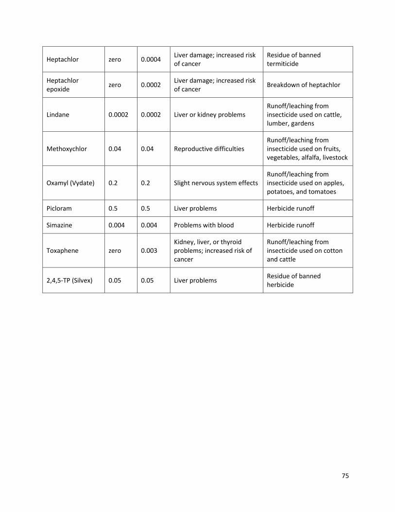
75

Heptachlor zero 0.0004 Liver damage; increased risk

of cancer

Residue of banned

termiticide

Heptachlor

epoxide

zero 0.0002 Liver damage; increased risk

of cancer Breakdown of heptachlor

Lindane 0.0002 0.0002 Liver or kidney problems

Runoff/leaching from

insecticide used on cattle,

lumber, gardens

Methoxychlor 0.04 0.04 Reproductive difficulties

Runoff/leaching from

insecticide used on fruits,

vegetables, alfalfa, livestock

Oxamyl (Vydate) 0.2 0.2 Slight nervous system effects

Runoff/leaching from

insecticide used on apples,

potatoes, and tomatoes

Picloram 0.5 0.5 Liver problems Herbicide runoff

Simazine 0.004 0.004 Problems with blood Herbicide runoff

Toxaphene zero 0.003

Kidney, liver, or thyroid

problems; increased risk of

cancer

Runoff/leaching from

insecticide used on cotton

and cattle

2,4,5-TP (Silvex) 0.05 0.05 Liver problems Residue of banned

herbicide

76

Appendix B: Price of Using Ozonation80 Ozone Economic Assumptions

Time Frame 20 Years

Power Cost 0.07 $/kWh

Interest Rate 5%

Ozone Production Rate 450 lbs/day (with 100% redundancy)

Ozone Concentration 2%

Power Consumption 10.1 kWh/lb ozone

Capital Cost $549,000

Ozone Concentration 10%

Power Consumption 4.5 kWh/lb ozone

LOX System Rental $1,000/month (tank, evaporators, valves and

controls)

77

Appendix C: Activated Carbon Adsorption Data All activated carbon experiments run for 24 hours

Alachlor

Sample

Volume

(mL)

Mass of

Pesticide

(mg) in

Sample

Mass of GAC

(g) in

Sample

Mass Ratio

(Adsorbate:

Adsorbant)

Absorbance

Equilibrium

Concentration

(mg/L)

Removal

Percentage

(%)

30 5.66 0.0028 0.5 0.3970 195.41 -4

30 5.66 0.0057 1.0 0.3405 168.12 11

30 5.66 0.0113 2.0 0.2610 129.72 31

30 5.66 0.0283 5.0 0.1629 82.33 56

30 5.66 0.0566 10.0 0.0041 5.62 97

25 4.72 0.0047 1.0 0.3820 188.17 0

30 4.00 0.0057 1.4 0.2265 113.05 40

20 2.67 0.0099 3.7 0.1309 66.87 65

20 2.67 0.0099 3.7 0.1186 60.93 68

30 5.66 0.0283 5.0 0.1484 75.32 60

20 2.73 0.0273 10.0 0.0361 21.08 89

20 2.73 0.0409 15.0 0.0201 13.35 93

20 2.67 0.0400 15.0 0.0350 20.55 89

20 2.73 0.0545 20.0 0.0168 11.76 94

20 2.73 0.0682 25.0 0.0019 4.56 98

15 2.00 0.0987 49.3 0.0087 7.84 96

Freundlich Isotherm for Alachlor

Loading

(mg/g) ln Loading 1/loading

Equilibrium Concentration

(mg/L)

ln Equ.

Conc

1/Equ

Conc

134.28 4.900 0.007 66.87 4.203 0.015

146.28 4.986 0.007 60.93 4.110 0.016

120.14 4.789 0.008 75.32 4.322 0.013

84.54 4.437 0.012 21.08 3.048 0.047

60.14 4.097 0.017 13.35 2.591 0.075

56.39 4.032 0.018 20.55 3.023 0.049

45.69 3.822 0.022 11.76 2.464 0.085

38.66 3.655 0.026 4.56 1.517 0.219

19.07 2.948 0.052 7.84 2.060 0.128

78

Slope is 0.5201 and y-intercept is 2.57. The natural log of the y-intercept is 13.01. The Freundlich

isotherm for alachlor is therefore:

S ���"FGFHIGJK � ������������ �������� �4.T 4� ∗ 13.01

Atrazine

Sample

Volume

(mL)

Mass of

Pesticide

(mg) in

Sample

Mass of GAC

(g) in

Sample

Mass Ratio

(Adsorbate/A

dsorbant)

Absorbance

Equilibrium

Concentration

(mg/L)

Removal

Percentage

(%)

20 0.010 0.5000 49920 0.0124 0.50 98

20 0.033 0.0077 230 0.0325 1.67 92

20 0.015 0.0500 3251 0.0170 0.77 96

20 0.200 0.0030 15 0.1754 10.00 53

20 0.024 0.7518 31169 0.0245 1.21 95

20 0.012 0.9990 83264 0.0141 0.60 97

20 0.014 1.5058 105938 0.0160 0.71 97

20 0.025 2.0021 81057 0.0250 1.24 94

40 0.083 0.0100 120 0.0395 2.08 90

40 0.520 0.0050 10 0.2270 13.01 39

40 0.684 0.0025 4 0.2970 17.09 21

Freundlich Isotherm for Atrazine

Loading

(mg/g)

ln

Loading 1/Loading

Equilibrium Concentration

(mg/L)

ln Equ.

Conc.

1/Equ.

Conc.

0.854 -0.158 1.171 0.501 -0.692 1.997

55.444 4.015 0.018 1.673 0.514 0.598

y = 0.5201x + 2.566

R² = 0.7559

0.000

1.000

2.000

3.000

4.000

5.000

6.000

0.000 1.000 2.000 3.000 4.000 5.000

ln l

oa

din

g

ln equilibrium concentration

Alachlor: Determination of Freundlich

Coefficients

79

8.538 2.145 0.117 0.769 -0.263 1.300

142.307 4.958 0.007 10.000 2.303 0.100

0.585 -0.536 1.709 1.206 0.187 0.829

0.440 -0.820 2.270 0.600 -0.511 1.667

0.292 -1.230 3.422 0.711 -0.342 1.407

0.220 -1.515 4.550 1.235 0.211 0.810

86.000 4.454 0.012 2.080 0.732 0.481

172.000 5.147 0.006 13.010 2.566 0.077

344.000 5.841 0.003 17.090 2.838 0.059

Slope is 0.6071 and y-intercept is 3.0466. The natural log of the y-intercept is 21.04. The Freundlich

isotherm for alachlor is therefore:

S ���"FLKFMN� � ������������ �������� �4.UV4� ∗ 21.04

Glyphosate

Sample

Volume

(mL)

Mass of

Pesticide

(mg) in

Sample

Mass of GAC

(g) in

Sample

Mass Ratio

(Adsorbate/A

dsorbant)

Absorbance

Equilibrium

Concentration

(mg/L)

Removal

Percentage

(%)

40 24 0.0024 0.1 0.0086 195.41 3.7

40 24 0.0024 0.1 0.0047 168.12 2.0

25 15 0.0030 0.2 0.0201 129.72 8.7

25 15 0.0075 0.5 0.0108 82.33 4.7

25 15 0.0075 0.5 0.0083 5.62 3.6

25 15 0.0150 1.0 0.0087 188.17 3.8

25 15 0.0150 1.0 0.0082 113.05 3.6

25 15 0.0300 2.0 0.0276 66.87 12.0

25 15 0.0750 5.0 0.0369 60.93 16.0

y = 0.6071x + 3.0466

R² = 0.7947

-2

0

2

4

6

8

10

-8 -6 -4 -2 0

ln L

oa

din

g

ln equilibrium concentration

Atrazine: Determination of

Freundlich Coefficients

80

25 15 0.0750 5.0 0.0361 75.32 15.7

20 12 0.1200 10.0 0.1045 21.08 45.4

20 12 0.1200 10.0 0.0341 13.35 14.8

20 12 0.1800 15.0 0.1165 20.55 50.7

15 9 0.1800 20.0 0.0268 11.76 11.7

15 9 0.2250 25.0 0.0182 4.56 7.9

15 9 0.2250 25.0 0.0175 7.84 7.6

Freundlich Isotherm for Glyphosate

Loading

(mg/g)

ln

Loading 1/loading Equilibrium Concentration (mg/L)

ln Equ.

Conc.

1/Equ

Conc

93.91 4.542 0.011 571.83 6.349 0.002

72.17 4.279 0.014 578.35 6.360 0.002

37.83 3.633 0.026 577.30 6.358 0.002

35.65 3.574 0.028 578.61 6.361 0.002

60.00 4.094 0.017 528.00 6.269 0.002

32.09 3.468 0.031 503.74 6.222 0.002

31.39 3.447 0.032 505.83 6.226 0.002

45.43 3.816 0.022 327.39 5.791 0.003

14.83 2.696 0.067 511.04 6.236 0.002

33.77 3.520 0.030 296.09 5.691 0.003

Slope is 0.3986 and y-intercept is 1.2415. The natural log of the y-intercept is 0.215. The Freundlich

isotherm for glyphosate is therefore:

S ���"OGPQIJRFL� � ������������ �������� �4.+WXU ∗ 0.215

y = 0.3985x + 1.2415

0.000

1.000

2.000

3.000

4.000

5.000

5.600 5.700 5.800 5.900 6.000 6.100 6.200 6.300 6.400

ln l

oa

din

g

ln equilibrium concentration

Glyphosate: Determination of

Freundlich Coefficients

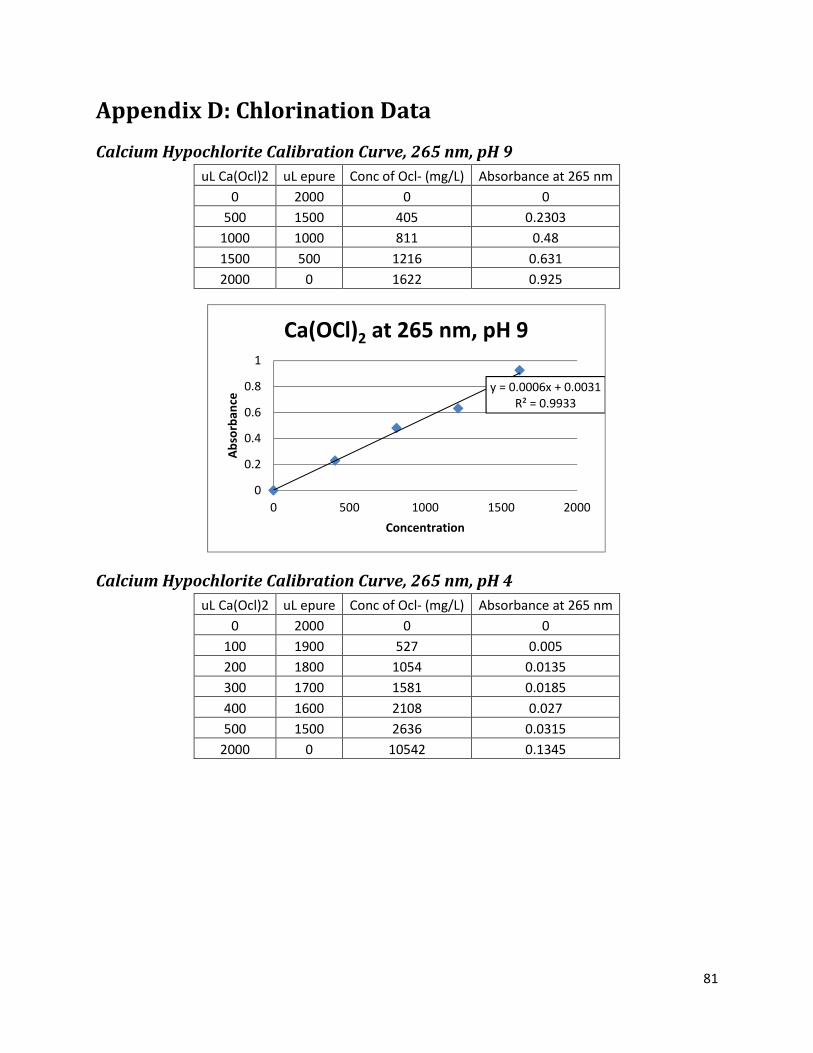
81

Appendix D: Chlorination Data

Calcium Hypochlorite Calibration Curve, 265 nm, pH 9

uL Ca(Ocl)2 uL epure Conc of Ocl- (mg/L) Absorbance at 265 nm

0 2000 0 0

500 1500 405 0.2303

1000 1000 811 0.48

1500 500 1216 0.631

2000 0 1622 0.925

Calcium Hypochlorite Calibration Curve, 265 nm, pH 4

uL Ca(Ocl)2 uL epure Conc of Ocl- (mg/L) Absorbance at 265 nm

0 2000 0 0

100 1900 527 0.005

200 1800 1054 0.0135

300 1700 1581 0.0185

400 1600 2108 0.027

500 1500 2636 0.0315

2000 0 10542 0.1345

y = 0.0006x + 0.0031

R² = 0.9933

0

0.2

0.4

0.6

0.8

1

0 500 1000 1500 2000

Ab

sorb

an

ce

Concentration

Ca(OCl)2 at 265 nm, pH 9

82

Calcium Hypochlorite Calibration Curve, 255 nm, pH 9

uL Ca(Ocl)2 uL epure Conc of Ocl- (mg/L) Absorbance at 255 nm

0 3000 0 0

500 2500 270 0.123

1000 2000 541 0.2815

1500 1500 811 0.409

2000 1000 1081 0.554

3000 0 1622 0.827

Calcium Hypochlorite Calibration Curve, 255 nm, pH 4

uL Ca(Ocl)2 uL epure Conc of Ocl- (mg/L) Absorbance at 255 nm

0 3000 0 0

100 2900 351 0.0043

200 2800 703 0.0096

300 2700 1054 0.013

y = 1E-05x - 0.0009

R² = 0.9995

-0.05

0

0.05

0.1

0.15

0 2000 4000 6000 8000 10000 12000

Ab

sorb

an

ce

Concentration

Ca(OCl)2 at 265 nm, pH 4

y = 0.0005x - 0.0044

R² = 0.9995

-0.2

0

0.2

0.4

0.6

0.8

1

0 500 1000 1500 2000

Ab

sorb

an

ce

Concentration

Ca(OCl)2 at 255 nm, pH 9

83

500 2500 1757 0.02

1000 2000 3514 0.042

Alachlor, pH 9

All initial alachlor concentrations 157.25 mg/L

Sample Volumes all 25 mL, corresponding to 0.015 mmoles alachlor

Molar

Ratio of

Ocl-

:Alachlor

mL of

Ca(Ocl)2

Added

Moles

Ocl-

Added

Absorbance

(24 hours)

Absorbance

Contribution

from All Ocl-

Added

Final

Concentration

(mg/L) Removing

all OCL-

%

Removal

1 0.049 0.000007 0.3280 0.0281 148.53 5.55

5 0.247 0.000036 0.4075 0.1269 139.19 11.48

10 0.494 0.000073 0.5055 0.2483 127.90 18.66

15 0.741 0.000109 0.5800 0.3673 106.38 32.35

25 1.235 0.000182 0.7260 0.5987 65.14 58.57

Alachlor, pH 4

All initial alachlor concentrations 157.25 mg/L

Sample Volumes all 10 mL, corresponding to 0.006 mmoles alachlor

Molar

Ratio of

Ocl-

:Alachlor

mL of

Ca(Ocl)2

Added

Moles

Ocl-

Added

Absorbance

(24 hours)

Absorbance

Contribution

from All Ocl-

Added

Final

Concentration

(mg/L) Removing

all OCL-

%

Removal

1 0.020 0.000003 0.3230 0.0013 159.03 -1.13

5 0.099 0.000015 0.3170 0.0112 151.35 3.75

10 0.198 0.000029 0.3420 0.0213 158.54 -0.82

15 0.296 0.000044 0.3330 0.0313 149.40 4.99

25 0.494 0.000073 0.3278 0.0505 137.57 12.51

y = 1E-05x + 0.0003

R² = 0.9979

0

0.01

0.02

0.03

0.04

0.05

0 1000 2000 3000 4000

Ab

sorb

an

ce

Concentration

Ca(OCl)2 at 255 nm, pH 4

84

Atrazine, pH 9

All initial alachlor concentrations 19.01 mg/L

Sample Volumes all 25 mL, corresponding to 0.002 mmoles atrazine

Molar

Ratio of

Ocl-

:Alachlor

mL of

Ca(Ocl)2

Added

Moles

Ocl-

Added

Absorbance

(24 hours)

Absorbance

Contribution

from All Ocl-

Added

Final

Concentration

(mg/L) Removing

all OCL-

%

Removal

1 0.007 0.000001 0.3283 0.0069 18.52 2.58

5 0.037 0.000006 0.3230 0.0220 17.33 8.82

10 0.075 0.000011 0.3300 0.0408 16.65 12.44

15 0.112 0.000017 0.3425 0.0596 16.28 14.35

25 0.187 0.000028 0.3915 0.0969 16.96 10.79

Atrazine, pH 4

All initial atrazine concentrations 19.01 mg/L

Sample Volumes all 15 mL, corresponding to 0.001 mmoles atrazine

Molar

Ratio of

Ocl-

:Alachlor

mL of

Ca(Ocl)2

Added

Moles

Ocl-

Added

Absorbance

(24 hours)

Absorbance

Contribution

from All Ocl-

Added

Final

Concentration

(mg/L) Removing

all OCL-

%

Removal

1 0.004 0.000001 0.3255 0.0010 18.70 1.63

5 0.022 0.000003 0.3345 0.0012 19.21 -1.04

10 0.045 0.000007 0.3271 0.0015 18.76 1.32

15 0.067 0.000010 0.3272 0.0018 18.75 1.38

25 0.112 0.000017 0.3225 0.0025 18.44 3.01

85

Appendix E: UV Photolysis/UV + H2O2 Data

Alachlor

Run 1 without H2O2

Sample sizes were 6 mL

Starting concentration of alachlor solution was 155.32 mg/L corresponding to an initial absorbance of

0.314

Contact Time (min) Absorbance Concentration (mg/L) % Absorbance Removal

0 0.314 155.32 0

15 1.090 530.16 -247.13

30 1.463 710.10 -365.76

60 1.605 778.98 -411.18

80 1.683 816.61 -435.99

Run 1 without H2O2

Sample sizes were 7 mL

Starting concentration of alachlor solution was 155.32 mg/L corresponding to an initial absorbance of

0.314

Contact Time (min) Absorbance Concentration (mg/L) % Absorbance Removal

0 0.314 155.32 0

30 1.518 736.91 -383.44

60 1.619 785.70 -415.61

90 1.690 819.99 -438.22

110 1.653 802.12 -426.43

125 1.419 688.85 -351.75

145 1.191 578.95 -279.30

215 0.927 451.19 -195.06

With H2O2

For the determination of which molar ratio of H2O2:alachlor to use

Sample sizes 6 mL total, starting concentration again 155.32 mg/L. Run for 45 minutes each.

Molar

Ratio

mL of H2O2

Added

Absorbance after 45

min

Concentration

(mg/L)

% Concentration

Removal

12.5 0.005 0.735 358.68 -139.12

25 0.010 0.0665 35.76 76.16

50 0.019 0.0693 37.12 75.26

100 0.039 0.1355 69.09 53.94

Using a 25:1 molar ratio of H2O2 : alachlor

86

Contact Time (min) Absorbance Concentration (mg/L) % Concentration Removal

0 0.3140 155.32 0

5 1.2709 617.55 -311.70

15 0.6125 299.51 -99.67

30 0.1509 76.53 48.98

45 0.0677 36.34 75.77

60 0.0300 18.13 87.91

75 0.0140 10.40 93.06

90 0.0092 8.08 94.61

105 0.0065 6.78 95.48

Atrazine

Without H2O2

Sample size was 5 mL with a starting atrazine concentration of 19 mg/L

Contact Time (min) Absorbance Concentration (mg/L) % Concentration Removal

0 0.33 19 0

16 0.219 12.544 34

30 0.1555 8.84 53

45 0.1063 5.97 69

60 0.071 3.9168 79

75 0.0465 2.488 87

90 0.0454 2.4245 87

With H2O2

A 100:1 molar ratio of H2O2:atrazine was used

The initial concentration of alachlor in solution was 21.93 mg/L

The sample size was 6 mL total

Contact Time (min) Absorbance Concentration (mg/L) % Concentration Removal

0 0.38 21.93 0

15 0.618 35.8 -63.2

60 0.205 11.73 46.5

90 0.068 3.74 82.9

120 0.037 1.93 91.2

87

Glyphosate

Without H2O2

A 25:1 molar ratio of H2O2:glyphosate was used

The initial concentration of glyphosate in solution was 695 mg/L

The sample size was 6 mL

Contact Time (min) Absorbance Concentration (mg/L) % Absorbance Removal

0 0.0141 695 0

30 0.0406 2020 -187.94

60 0.0563 2805 -299.29

90 0.0727 3625 -415.60

120 0.0851 4245 -503.55

With H2O2

A 25:1 molar ratio of H2O2:glyphosate was used

The initial concentration of glyphosate in solution was 1086 mg/L

The sample size was 6 mL

Contact Time (min) Absorbance Concentration (mg/L) % Concentration Removal

0 0.02 1085.78 0

15 0.19 10370.16 -855

30 0.15 8185.6 -654

45 0.12 6547.18 -503

60 0.07 3816.48 -251

75 0.05 2724.2 -151

90 0.01 539.64 50

88

Appendix F: Ozonation Data

Alachlor

Initial concentration of all alachlor samples was 155.32 mg/L, all sample sizes 75 mL

Contact Time (min) Absorbance % Absorbance Removal

0 0.314 0.00

5 0.3682 -17.26

15 0.456 -45.22

30 0.4390 -39.81

60 0.471 -49.84

90 0.4680 -49.04

Atrazine

Initial concentration of all atrazine samples was 18.2 mg/L, all sample sizes 75 mL

Contact Time (min) Absorbance Final Concentration (mg/L) % Concentration Removal

0 0.05495 18.2 0.00

15 0.06373 15.69 13.79

32 0.06619 15.11 16.98

60 0.06631 15.08 17.14

Appendix G: Kinetics Analysis Data

Ozonation Rate

Ozonation of Atrazine

14

15

16

17

18

19

0 10 20 30 40 50 60

Eq

uil

ibri

um

Co

nce

ntr

ati

on

(m

g/L

)

Contact Time (min)

Concentration of Atrazine versus

Time

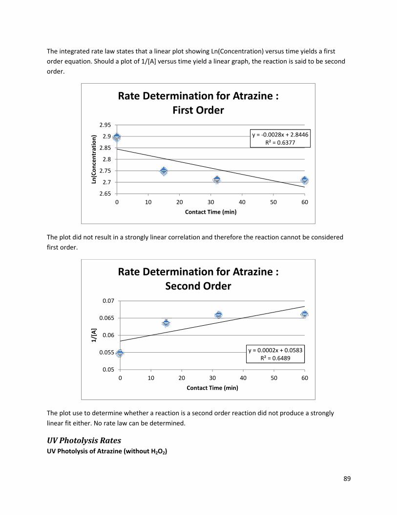
89

The integrated rate law states that a linear plot showing Ln(Concentration) versus time yields a first

order equation. Should a plot of 1/[A] versus time yield a linear graph, the reaction is said to be second

order.

The plot did not result in a strongly linear correlation and therefore the reaction cannot be considered

first order.

The plot use to determine whether a reaction is a second order reaction did not produce a strongly

linear fit either. No rate law can be determined.

UV Photolysis Rates

UV Photolysis of Atrazine (without H2O2)

y = -0.0028x + 2.8446

R² = 0.6377

2.65

2.7

2.75

2.8

2.85

2.9

2.95

0 10 20 30 40 50 60

Ln(C

on

cen

tra

tio

n)

Contact Time (min)

Rate Determination for Atrazine :

First Order

y = 0.0002x + 0.0583

R² = 0.6489

0.05

0.055

0.06

0.065

0.07

0 10 20 30 40 50 60

1/[

A]

Contact Time (min)

Rate Determination for Atrazine :

Second Order

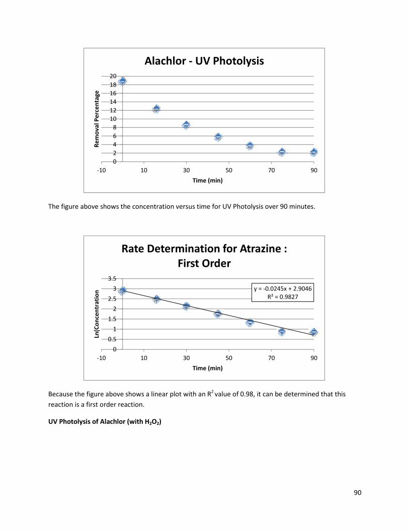
90

The figure above shows the concentration versus time for UV Photolysis over 90 minutes.

Because the figure above shows a linear plot with an R2 value of 0.98, it can be determined that this

reaction is a first order reaction.

UV Photolysis of Alachlor (with H2O2)

0

2

4

6

8

10

12

14

16

18

20

-10 10 30 50 70 90

Re

mo

va

l P

erc

en

tag

e

Time (min)

Alachlor - UV Photolysis

y = -0.0245x + 2.9046

R² = 0.9827

0

0.5

1

1.5

2

2.5

3

3.5

-10 10 30 50 70 90

Ln(C

on

cen

tra

tio

n

Time (min)

Rate Determination for Atrazine :

First Order

91

The figure above shows the logarithmic trend or the absorbance of alachlor to the contact time.

With an R2 value of 0.96, the reaction was determined to be first order.

UV Photolysis of Atrazine (with H2O2)

0

0.2

0.4

0.6

0.8

1

1.2

1.4

0 20 40 60 80 100

Ab

sorb

an

ce a

t 2

65

nm

UV Contact Time (min)

Alachlor - UV + H2O2

y = -0.0535x + 0.0516

R² = 0.9623

-6

-5

-4

-3

-2

-1

0

1

-10 10 30 50 70 90 110

Ln(C

on

cen

tra

tio

n)

UV Contact Time (min)

Rate Determination for Alachlor: First

Order

92

The figure above shows the correlation between the Absorbance and contact time.

Taking into account the spike at time twenty, the reaction was considered to be first order due to the

linearity of the plot.

UV Photolysis of Glyphosate (with H2O2)

0

0.1

0.2

0.3

0.4

0.5

0.6

0.7

0 20 40 60 80 100 120

Ab

sorb

an

ce (

nm

)

Time (min)

Atrazine - UV + H2O2

y = -0.0232x + 3.5438

R² = 0.9189

0

0.5

1

1.5

2

2.5

3

3.5

4

0 20 40 60 80 100 120

Ln(C

on

cen

tra

tio

n)

Time (min)

Rate Determination for Atrazine :

First Order

93

The above figure shows how after the initial spike of in the absorbance reading at approximately time

equals ten minutes, the absorbance decreases in a linear fashion.

When all data points after the initial spike are analyzed, it is clear that the reaction of byproducts and

glyphosate follow a typical zeroth order reaction.

0

0.05

0.1

0.15

0.2

0 20 40 60 80 100

Ab

sorb

an

ce R

ea

din

g

Contact Time (min)

Glyphosate - UV + H2O2

y = -0.0024x + 0.2233

R² = 0.9928

0

0.05

0.1

0.15

0.2

0 20 40 60 80 100

Ab

sorb

an

ce R

ea

din

g

Contact Time (min)

Rate Determination for Glyphosate:

Zeroth Order