perturbation analysis for the reduced minimum modulus of bounded linear operator in banach spaces

Applied Mathematics and Computation 145 (2003) 13–21

www.elsevier.com/locate/amc

Perturbation analysis for the reducedminimum modulus of bounded linear

operator in Banach spaces q

Chao Zhu, Jing Cai, Guo-liang Chen *

Department of Mathematics, East China Normal University, Shanghai 200062, China

Abstract

Let X and Y be two Banach spaces over the complex field C and let T : X ! Y be a

bounded linear operator with the generalized inverse Tþ. Let T ¼ T þ dT be a bounded

linear operator with kTþkkdTk < 1=2. Let cðT Þ denote the reduced minimum modulus

of T. We first establish the upper semi-continuity theorem for cðT Þ. Furthermore, if

dimKer T ¼ dim KerT < þ1 orRðT Þ \KerTþ ¼ 0, then cðT Þ is continuous under theoperator norm. Also, we have a corollary in Hilbert spaces, which improves the result in

[Linear Algebra Appl., 262 (1997) 229–242, Theorem 4.1].

� 2002 Published by Elsevier Inc.

Keywords: Generalized inverse; Reduced minimum modulus; Stable perturbation of operators

1. Introduction

Let X and Y be two Banach spaces over the complex field C and let

T : X ! Y be a bounded linear operator with the generalized inverse Tþ. In this

paper, we shall consider the upper semi-continuity or continuity of cðT Þ underoperator norm, where cðT Þ denote the reduced minimum modulus of T.

qProject supported by National Natural Science Foundation of China (no. 19871029) and

Shanghai Priority Academic Discipline Foundation.* Corresponding author.

E-mail address: [email protected] (G.-l. Chen).

0096-3003/02/$ - see front matter � 2002 Published by Elsevier Inc.

doi:10.1016/S0096-3003(02)00434-4

mail to: [email protected]

14 C. Zhu et al. / Appl. Math. Comput. 145 (2003) 13–21

Kato introduced the conception of the reduced minimum modulus cðT Þ in[8], which later shows its vital importance in perturbation analysis for linearoperators. Ding and Huang [5,6] and Chen and Xue [2,3] have presented

several results about cðT Þ. Ding and Huang [7] has proved that cðT Þ is uppersemi-continuous in Hilbert spaces. While in this paper, we aim to generalize

the result to more general Banach spaces. Furthermore, if dimKer T ¼dim KerT < þ1 or RðT Þ \KerTþ ¼ 0, then cðT Þ is continuous. Also, we get

a corollary in Hilbert spaces, which improves the result in [7, Theorem 4.1].

After introducing some concepts in the next section, we present the main

result in Section 3. Conclusions will be arranged in Section 4.The notation used in this paper are the same of those in [1]. For the basic

properties of linear operators, please see [10] or [8].

2. Preliminaries

Let X and Y be two Banach spaces over the complex field C and let BðX ; Y Þdenote the Banach spaces of all bounded linear operators T : X ! Y with the

norm kTk ¼ supfkTxk : kxk ¼ 1; x 2 Xg, where k � k is the norm of X or Y. ForT 2 BðX ; Y Þ, Ker T denotes the null space and RðT Þ denotes the range of T,

respectively. Let T 2 BðX ; Y Þ with RðT Þ closed. If there exist two bounded

projections (idempotents) of P : X ! KerT ;Q : Y ! RðT Þ, then T has the

unique generalized inverse Tþ ¼ TþP Q (with respect to P ;Q) such that

TTþT ¼ T ; TþTTþ ¼ Tþ; TþT ¼ I P ; TTþ ¼ Q: ð1Þ

If X and Y are Hilbert spaces, we require ðTþT Þ� ¼ TþT , ðTTþÞ� ¼ TTþ in (1)

(see [9] for more details).

Let T 2 BðX ; Y Þ, the reduced minimum modulus cðT Þ of T is defined by

cðT Þ ¼ inffkTxk : distðx;KerT Þ ¼ 1; x 2 Xg ð2Þ

Thus from the definition of cðT Þ, we deduce that

kTxkP cðT Þdistðx;KerT Þ for any x 2 X :

Proposition 2.1. Let T 2 BðX ; Y Þ, then

(a) cðT Þ > 0 if and only if RðT Þ is closed;(b) cðT �Þ ¼ cðT Þ, where T � is the adjoint of T.

For proof of the proposition, see [8, Theorem 5.13 and Theorem 5.2].

Lemma 2.1. Let T 2 BðX ; Y Þ with the generalized inverse Tþ, then

C. Zhu et al. / Appl. Math. Comput. 145 (2003) 13–21 15

1

kTþk 6 cðT Þ6 kTk: ð3Þ

Proof. For any x 2 X ; y 2 KerT ,

kTþTxk ¼ kTþT ðx yÞk6 kTþTkkx yk ð4Þ

distðx;KerT Þ6 kx ðI TþT Þxk ¼ kTþTxk:

Thus,

kTþkkTxkP kTþTxkP distðx;KerT Þ: ð5Þ

Combining the definition of cðT Þ and (5), we have cðT ÞP 1=kTþk. From (4),

we have

kx ykPkTþTxkkTþTk for any x 2 X ; y 2 KerT ;

hence

distðx;KerT ÞPkTþTxkkTþTk :

Therefore

kTxkP cðT Þdistðx;KerT ÞP cðT Þ kTþTxk

kTþT k for any x 2 X

so kT kP cðT Þ. Thus we have proved Lemma 2.1. �

Remark 2.1. If X ; Y are Hilbert spaces, then cðT Þ ¼ 1=kTþk (see [5] for proof).

In this case, Lemma 2.1 is still right, since kTk=cðT Þ ¼ kTkkTþkP kTTþk ¼ 1.

Suppose X is a Banach space, for any two subspaces A and B of X, the gapbetween A and B : dðA;BÞ is defined as

dðA;BÞ ¼ supfdistðx;BÞ : kxk ¼ 1; x 2 Ag:

Lemma 2.2. Let T 2 BðX ; Y Þ with the generalized inverse Tþ and letT ¼ T þ dT 2 BðX ; Y Þ, then

cðT ÞdðKerT ;KerT Þ6 kdTk: ð6Þ

Proof. For any u 2 KerT with kuk ¼ 1, we have Tu ¼ dT ð uÞ. Thus
kdTkP kdT ð uÞk ¼ kTukP cðT Þdistðu;KerT Þ;
hence

kdTkP cðT ÞdðKerT ;KerT Þ: �


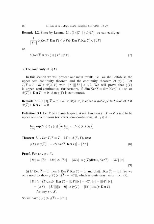
Remark 2.2. Since by Lemma 2.1, ð1=kTþkÞ6 cðT Þ, we can easily get

1

kTþk dðKerT ;KerT Þ6 cðT ÞdðKerT ;KerT Þ6 kdTk

or

dðKerT ;KerT Þ6 kTþkkdTk: ð7Þ

3. The continuity of cðTÞ

In this section we will present our main results, i.e., we shall establish the

upper semi-continuity theorem and the continuity theorem of cðT Þ. Let

T ; T ¼ T þ dT 2 BðX ; Y Þ with kTþkkdT k < 1=2. We will prove that cðT Þis upper semi-continuous; furthermore, if dimKer T ¼ dim KerT < þ1 orRðT Þ \KerTþ ¼ 0, then cðT Þ is continuous.

Remark 3.1. In [3], T ¼ T þ dT 2 BðX ; Y Þ is called a stable perturbation of T if

RðT Þ \KerTþ ¼ 0.

Definition 3.1. Let X be a Banach space. A real function f : X ! R is said to be

upper semi-continuous (or lower semi-continuous) at x0 2 X if

limx!x0

sup f ðxÞ6 f ðx0Þ�or lim

x!x0inf f ðxÞP f ðx0Þ

�:

Theorem 3.1. Let T ; T ¼ T þ dT 2 BðX ; Y Þ, then

cðT ÞP cðT Þ½1 2dðKerT ;KerT Þ� kdT k: ð8Þ

Proof. For any x 2 X ,

kTxk ¼ kT x dTxkP kT xk kdTxkP cðT Þdistðx;KerT Þ kdTkkxk:ð9Þ

(i) If Ker T ¼ 0, then dðKerT ;KerT Þ ¼ 0, and distðx;KerT Þ ¼ kxk. So we

only need to show cðT ÞP cðT Þ kdTk, which is quite easy, since from (9),

kTxkP cðT Þdistðx;KerT Þ kdTkkxk ¼ cðT Þkxk kdTkkxk¼ ðcðT Þ kdT kÞkx 0kP ðcðT Þ kdTkÞdistðx;KerT Þfor any x 2 X :

So we have cðT ÞP cðT Þ kdT k.


(ii) If Ker T 6¼ 0, from the definition of cðT Þ, we know that there exists a

sequence fxng1n¼1 � X such that distðxn;KerT Þ ¼ 1 and limn!þ1 kTxnk ¼ cðT Þ.Then for any given positive number �, there is a sequence fyng1n¼1 � KerT , suchthat

16 kxn ynk < 1þ �: ð10Þ

Choose a sequence fzng1n¼1 � KerT ðzn 6¼ 0Þ such that

kxn ynkP distðxn yn;KerT Þ > kxn yn znk �: ð11Þ

For any z 2 KerT , we have

kxn yn znkP kxn zk kyn þ zn zkP distðxn;KerT Þ

kznkzn

kznk

�� þ yn zkznk

�� ¼ 1 kznkzn

kznk

�� þ yn zkznk

��: ð12Þ

On the other hand, from (10) and (11),

kznk ¼ kðxn yn znÞ ðxn ynÞk6 kðxn yn znÞk þ kxn ynk< ð�þ kxn ynkÞ þ kxn ynk < �þ 2ð1þ �Þ ¼ 2þ 3�: ð13Þ

Hence, combining (11)–(13), we have

dist ðxn yn;KerT Þ þ � > kxn yn znkP 1 ð2þ 3�Þ znkznk

�� þ yn zkznk

��for any z 2 KerT

so,

dist ðxn yn;KerT Þ þ �P 1 ð2þ 3�Þdist znkznk

;KerT� �

P 1 ð2þ 3�ÞdðKerT ;KerT Þ: ð14Þ

Therefore, from (9), (10) and (14), we have

kTxnk ¼ kT ðxn ynÞkP cðT Þdistðxn yn;KerT Þ kdTkkxn ynkP cðT Þ½1 ð2þ 3�ÞdðKerT ;KerT Þ� ð1þ �ÞkdTk: ð15Þ

Let � ! 0 in (15), we have

kTxnkP cðT Þ½1 2dðKerT ;KerT Þ� kdT k ð16Þ

and let n ! 1 in (16), we have

cðT ÞP cðT Þ½1 2dðKerT ;KerT Þ� kdT k: �

If we denote dðKerT ;KerT Þ ¼ maxfdðKerT ;KerT Þ; dðKerT ;KerT Þg, thenwe have the following corollary:


Corollary 3.1. Let T ; T be as in Theorem 3.1, then

jcðT Þ cðT Þj6 2maxfcðT Þ; cðT ÞgdðKerT ;KerT Þ þ kdT k: ð17Þ

Proof. By simple computation from (8), we have

cðT Þ cðT Þ6 2cðT ÞdðKerT ;KerT Þ þ kdTk: ð18Þ

Interchange T ; T in (18), and we have

cðT Þ cðT Þ6 2cðT ÞdðKerT ;KerT Þ þ kdTk

or

cðT Þ cðT ÞP ½2cðT ÞdðKerT ;KerT Þ þ kdTk�: ð19Þ

Then the combination of (18) and (19) is (17). �

The following corollary is evident.

Corollary 3.2. Let T ; T be as in Theorem 3.1. Assume that Ker T ¼ KerT , thenjcðT Þ cðT Þj6 kdT k.

Let BcðX ; Y Þ denote the set of all bounded linear operators T : X ! Y with

the generalized inverse Tþ. Let T ¼ T þ dT 2 BðX ; Y Þ with kTþkkdTk < 1=2.The following theorem will show that c : ðBcðX ; Y Þ; k kÞ ! Rþ is upper semi-

continuous.

Theorem 3.2. Suppose that kTþkkdTk < 1=2, then c : ðBcðX ; Y Þ; k � kÞ ! Rþ isupper semi-continuous.

Proof. From Theorem 3.1, we have

cðT ÞP cðT Þ½1 2dðKerT ;KerT Þ� kdT k:

From (7),

dðKerT ;KerT Þ6 kTþkkdTk <1

2

so

1 2dðKerT ;KerT Þ > 0

so we have

cðT Þ6 cðT Þ þ kdTk1 2dðKerT ;KerT Þ

;


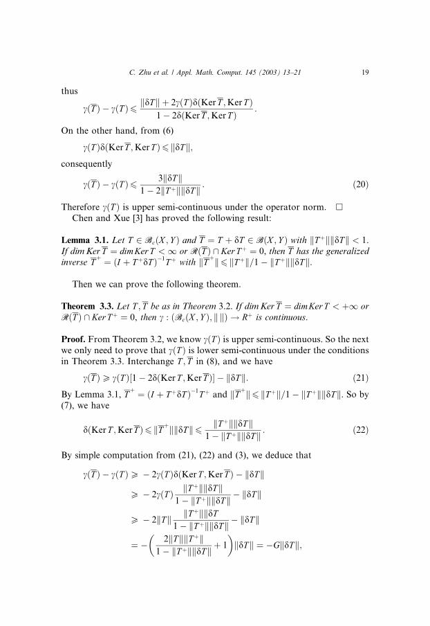
thus

cðT Þ cðT Þ6 kdTk þ 2cðT ÞdðKerT ;KerT Þ1 2dðKerT ;KerT Þ

:

On the other hand, from (6)

cðT ÞdðKerT ;KerT Þ6 kdTk;

consequently

cðT Þ cðT Þ6 3kdTk1 2kTþkkdTk : ð20Þ

Therefore cðT Þ is upper semi-continuous under the operator norm. �

Chen and Xue [3] has proved the following result:

Lemma 3.1. Let T 2 BcðX ; Y Þ and T ¼ T þ dT 2 BðX ; Y Þ with kTþkkdTk < 1.If dimKer T ¼ dimKer T < 1 or RðT Þ \ KerTþ ¼ 0, then T has the generalizedinverse T

þ ¼ ðI þ TþdT Þ 1Tþ with kTþk6 kTþk=1 kTþkkdTk.

Then we can prove the following theorem.

Theorem 3.3. Let T ; T be as in Theorem 3.2. If dimKer T ¼ dimKer T < þ1 orRðT Þ \ KerTþ ¼ 0, then c : ðBcðX ; Y Þ; k kÞ ! Rþ is continuous.

Proof. From Theorem 3.2, we know cðT Þ is upper semi-continuous. So the next

we only need to prove that cðT Þ is lower semi-continuous under the conditions

in Theorem 3.3. Interchange T ; T in (8), and we have

cðT ÞP cðT Þ½1 2dðKerT ;KerT Þ� kdT k: ð21Þ

By Lemma 3.1, Tþ ¼ ðI þ TþdT Þ 1Tþ and kTþk6 kTþk=1 kTþkkdTk. So by

(7), we have

dðKerT ;KerT Þ6 kTþkkdTk6 kTþkkdT k1 kTþkkdTk : ð22Þ

By simple computation from (21), (22) and (3), we deduce that

cðT Þ cðT ÞP 2cðT ÞdðKerT ;KerT Þ kdTk

P 2cðT Þ kTþkkdTk1 kTþkkdTk kdTk

P 2kTk kTþkkdT1 kTþkkdTk kdTk

¼ 2kTkkTþk1 kTþkkdT k

�þ 1

�kdTk ¼ GkdTk;


where G ¼ ð2kT kkTþk=1 kTþkkdT k þ 1Þ is a bounded positive number since

kTþkkdT k < 1=2. So cðT Þ is lower semi-continuous under the operator norm.Then we complete the proof of Theorem 3.3. �

In the end of the section, we shall consider the problem that whether our

results in the previous are still valid in Hilbert spaces. Obviously, Theorems 3.1

and 3.2 are right in Hilbert spaces. As for Theorem 3.3, things are somehow

different, since Tþ ¼ ðI þ TþdT Þ 1Tþ is not necessarily the generalized inverse

of T in Hilbert spaces (see [4] for details). Fortunately, Chen and Xue [4] has

proved the following result:

Lemma 3.2. Let X, Y be two Hilbert spaces over the complex field and letT : X ! Y be a bounded linear operator with the generalized inverse Tþ and letT ¼ T þ dT 2 BðX ; Y Þ with kTþkkdTk < 1. Suppose that dimKer T ¼ dimKerT< þ1 or RðT Þ \ KerTþ ¼ 0. Then T has the generalized inverse T

þwith

kTþk6 kTþk=1 kTþkkdTk.

Hence we still have the inequality (22) in Hilbert spaces:

dðKerT ;KerT Þ6 kTþkkdTk6 kTþkkdT k1 kTþkkdTk ;

therefore the deducements in Theorem 3.3 are still valid if X ; Y are Hilbert

spaces. Thus we have the following corollary:

Corollary 3.3. If X,Y are two Hilbert spaces, then Theorems 3.1, 3.2 and 3.3 arestill valid.

Till now we have solved the problem, and our results do improve Ding and

Huang�s work in [7, Theorem 4.1].

4. Conclusions

In this paper, we have established several perturbation theories of the re-

duced minimum modulus of bounded linear operator in Banach spaces, and we

can have Theorem 4.1 in [7] as a natural corollary of our results, we also have

improved Ding and Huang�s work.It is quite well known that the reduced minimum modulus is of vital im-

portance in perturbation analysis for linear operators. We will investigate the

applications of our results in the future.


Acknowledgements

We really appreciate Prof. Yi-feng Xue for his great help in the proof of

Theorem 3.1. We also thank referees for their useful suggestions and com-

ments.

References

[1] A. Ben-Israel, T.N.E. Greville, Generalized Inverse: Theory and Applications, Wiley, New

York, 1974.

[2] G.L. Chen, M.S. Wei, Y.F. Xue, Perturbation analysis of the least solution in Hilbert spaces,

Linear Algebra Appl. 244 (1996) 69–80.

[3] G.L. Chen, Y.F. Xue, Perturbation analysis for the operator equation Tx ¼ b in Banach

spaces, J. Math. Anal. Appl. 212 (1997) 107–125.

[4] G.L. Chen, Y.F. Xue, The expression of the generalized inverse of the perturbed operator

under Type I perturbation in Hilbert spaces, Linear Algebra Appl. 285 (1998) 1–6.

[5] J. Ding, L.J. Huang, On the perturbation of the least squares solution in Hilbert spaces, Linear

Algebra Appl. 212/213 (1994) 487–500.

[6] J. Ding, L.J. Huang, Perturbation of generalized inverse of linear operators in Hilbert spaces,

J. Math. Anal. Appl. 198 (1996) 506–515.

[7] J. Ding, L.J. Huang, On the continuity of generalized inverse of linear operators in Hilbert

spaces, Linear Algebra Appl. 262 (1997) 229–242.

[8] T. Kato, Perturbation Theory for Linear Operators, Springer-Verlag, New York, 1984.

[9] M.Z. Nashed, Perturbations and approximations for generalized inverse and linear operator

equations, in: M.Z. Nashed (Ed.), Generalized Inverse and Applications, Academic press, New

York, 1976.

[10] K. Yosida, Functional Analysis, Springer-Verlag, New York, 1978.

perturbation analysis for the reduced minimum modulus of bounded linear operator in banach spaces

Documents