perspectives in biometry || on parameter estimation and goodness-of-fit testing for spatial point...

On Parameter Estimation and Goodness-of-Fit Testing for Spatial Point PatternsAuthor(s): Peter J. DiggleSource: Biometrics, Vol. 35, No. 1, Perspectives in Biometry (Mar., 1979), pp. 87-101Published by: International Biometric SocietyStable URL: http://www.jstor.org/stable/2529938 .

Accessed: 28/06/2014 09:17

Your use of the JSTOR archive indicates your acceptance of the Terms & Conditions of Use, available at .http://www.jstor.org/page/info/about/policies/terms.jsp

.JSTOR is a not-for-profit service that helps scholars, researchers, and students discover, use, and build upon a wide range ofcontent in a trusted digital archive. We use information technology and tools to increase productivity and facilitate new formsof scholarship. For more information about JSTOR, please contact [email protected].

.

International Biometric Society is collaborating with JSTOR to digitize, preserve and extend access toBiometrics.

http://www.jstor.org

This content downloaded from 78.24.216.166 on Sat, 28 Jun 2014 09:17:51 AMAll use subject to JSTOR Terms and Conditions

http://www.jstor.org/action/showPublisher?publisherCode=ibs

http://www.jstor.org/stable/2529938?origin=JSTOR-pdf

http://www.jstor.org/page/info/about/policies/terms.jsp


Ke Words. Spatial point pattern; Spatial point process; Monte Carlo test; EGO10gY; Goodness-offit; Parameter estimation.

BIOMETRICS 35, 87-101 M arch, 1 979

On Paratneter Estitnation and Goodnessof-fit Testing for Spatial Point Patterns

PETER J. DIGGLE

Department of Statistics, University of Newcastle upon Tyne, Newcastle upon Tyne N E 1 7RU, England

Summary

The paper discusses the objectives of spatial point pattern analsis with particular reference to the distinction between mapped and sampled data. For the former case available nlodels are reviewed briefly the role of preliminary testing is discussed and a procedure for ftting a parametric sslodel is outlined. A simulation studA of several tests of spatial randonlness is intended to provide some insight into the suitability for model-fitting of various summasy descriptions of a mapped pattern. Two examples illustrate the use of the statistical techniques. Soss1e problem areas which-merit further investigation are identified.

1. Intsoduction Studies of an irregular spatial distribution of point locations, henceforth events, arise in

many branches of biology, but predominantly in ecology. See, for example, Greig-Smith (1964). In the development of an appropriate statistical methodology it is important to preserve a clear distinction between data presented as a complete map of events in some essentially planar region, and data derived from sparse sampling in the field, whether in the form of counts in randomly located quadrats or variously defined distances from randomly located points to neighbouring events. In practice, but with reservations noted by Holgate (1965), analyses of sparsely sampled patterns can safely assume that observations from diCerent sampling points are mutually independent. ln contrast, the exhaustive sampling of a mapped pattern almost invariably generates a set of dependent observations.

Analyses of sparsely sampled patterns are usually confined to testing the hypothesis of complete spatial randomness and estimating the intensity, or mean number of events per unit area. This seems quite proper in view of the fact that sparse sampling cannot provide an adequate checld on the assumptions required for the more sophisticated type of analysis considered below.

When mapped data are available, tests of complete spatial randomness remain useful as a means towards the identification of interesting features of the data, very much in the spirit of Mead's (1974) use of contiguous quadrat counts, but such tests may now be followed in appropriate cases by the fitting of model within some specified parametric class, as in the important paper of Ripley (1977). The purpose of such model-fitting is, in the first instance, to provide a quantitative description of pattern as a basis for the comparison of ostensibly similar datasets (c.f. Besag 1977a). A more ambitious objective is to establish a plausible

87



88 BIOMETRICS, MARCH 1979

biological mechanism whereby the data may have been generated, although without additional information on possible environmental variation, temporal development, etc. and especially for observational rather than experimental studies, definitive conclusions cannot be expected.

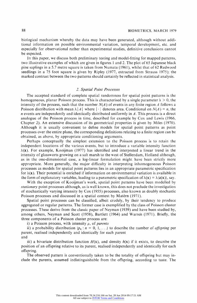
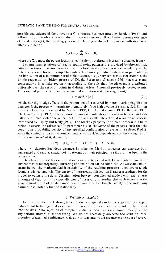
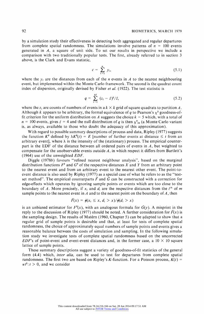
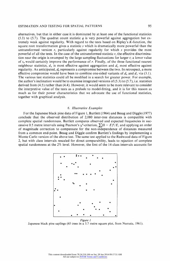
In this paper, we discuss both preliminary testing and model-fitting for mapped patterns, two illustrative examples of which are given in figures 1 and 2. The plot of 65 Japanese black pine saplings in a 5.7 metre square is taken from Numata (1961)9 whilst that of 62 Redwood seedlings in a 75 foot square is given by Ripley (1977, extracted from Strauss 1975); the marked contrast between the two patterns should certainly be reflected in statistical analysis.

2. Spatiat Point Processes The accepted standard of complete spatial randomness for spatial point patterns is the

homogeneous, planar Poisson process. This is characterised by a single parameter X > 0, the intensity of the process, such that the number N(A ) of events in any finite region A follows a Poisson distribution with mean X | A | where | | denotes area. Conditional on N(A ) = n, the n events are independently and identically distributed uniformly in A. This process is a direct analogue of the Poisson process in time, described for example by CCox and Lewis (19669 Chapter 2). An extensive discussion of its geometrical properties is given by Miles (1970). Although it is usually convenient to define models for spatial point patterns as poin processes over the entire plane, the corresponding dehI1itions relating to a finite region can be obtained, as above, by appropriate conditionirlg arguments.

Perhaps conceptually the simplest extension to the Poisson process is to retain the indeperldent locations of the various events, but to introduce a variable intensity function A(x). For example, Kooijman (1977) has identified and interpreted a linear trend in the intensity of glassworts growing on a salt marsh to the west vf Stellerldam, lHolland although, as in the one-dimensional case, a log linear formulation might have been strictly more appropriate. More generally, the major difficulty in interpreting inhomogeneous Poisson processes as models for spatial point patterns lies in an appropriate parametric specification for A(x). Their potential is enriched if information on environmental variation is available in the form of explanatory variables, leading to a parametric specification of A(x) - A{z(X)}9 say.

With the exception of Kooijman's work, spatial point patterrls have been modelled by stationary point processes although, as is well known, this does not preclude the investigation of stochastically varying intensity by Cox (1955) processes, also known as doubly stochastic Poisson processes and discussed in a spatial context by Matern (1971).

Spatial point processes can be classified9 albeit crudely, by their tendency to produee aggregated or regular patterns. The former case is exemplified by the class of Poisson cluster proeesses. These derive from the classie paper of Neyman (i939) and have been studied by, among others9 Neyman and Scott (1958), Bartlett (1964) and Warrerl (1971). Briefly9 the three components of a Poisson cluster process are:

i) a Poisson process, with intensity p, of parents

ii) a probability distribution {Pn: n = O, 1, . . .} to describe the number of oJfspring per parent, realised independently and identically for each parent and

iii) a bivariate distribution fun&tion H(x), and density h(x) if it exists, to deseribe the position of an oWspring relative to its parent, realised independently and identically for each oWspritlg.

The observed pattern is eonventionally taken to be the totality of oWspring but may in GIUt the parents, assumed indistinguishable from the oWspring, aceording to tastee The



ESTIMATION AND TESTING FOR SPATIAL PATTERNS 89

possible equivalence of the above to a Cox process has been noted by Bartlett (1964), and follows if {Pn} describes a Poisson distribution with mean ,u. If we further assume existence of the density h(x), the resulting process of offspring is also a Cox process with stochastic intensity function

co

(X) = ,u £ h(x- Xi), i=l

where the Xi denote the parent locations, conveniently ordered in increasing distance from x. Extreme manifestations of regular spatial point patterns are provided by deterministic

lattice structures. It seems more natural in a biological context to model regularity as the outcome of some form of competitive interaction amongst individuals, and in particular by the imposition of a minimum permissible distance, 6 say, between events. For example, the simple sequential inhibition process of Diggle, Besag and Gleaves (1976) places n events consecutively in a finite region A according to the rule that the ith event is distributed uniformly over the set of all points in A distant at least 6 from all previously located events. The essential parameter of simple sequential inhibition is its packing density,

r = nzzb2/4|A| (2.1)

which, bar slight edge-effects, is the proportion of A covered by n non-overlapping discs of diameter b; the process will terminate prematurely if too high a value of r is specified. Similar processes have been described by Matern (1960, Ch. 3), Paloheimo (1971), Bartlett (1975, Ch. 1) and Ripley (1977). The extension to non-rigid inhibitory interactions between individuals is subsumed within the general definition of a locally interactive Markov point process, introduced by Ripley and Kelly (1977). The Markov property for a point process in a finite region A asserts the existence of a parameter 6 > 0, the range of the process, such that the conditional probability density of any specified configuration of events in a subset B of A, given the configuration in the complementary region A /B, depends only on the configuration in the environment of B, defined by

E(B) = {x E A/B: H y E B, IIY-X|| < 6} where 11 11 denotes Euclidean distance. In principle, Markov processes can embrace both aggregated and regular spatial point patterns, but their principal use thus far has been in the latter context.

The classes of models described above can be extended at will. In particular, elements of environmental heterogeneity, clustering and inhibition can be combined. As we shall demonstrate below, the mathematical intractability of the resulting processes does not preclude formal statistical analysis. The danger of increased sophistication is rather a tendency for the model to outstrip the data. Discrimination between complicated models will require large amounts of data, but it is especially true of observational studies that each increase in the geographical extent of the data imposes additional strain on the plausibility of the underlying assumptions, notably that of stationarity.

3. Preliminary A nalysis

As noted in Section 1 above, tests of complete spatial randomness applied to mapped data are not to be regarded as an end in themselves, but can help to provide useful insight into the data. Also, rejection of complete spatial randomness is a minimal pre-requisite to any serious attempt at model-fitting. We do not necessarily advocate too strict an interpretation of attained significance levels at this stage and would recommend the use of several



9o BIOMETRICS, MARCH 1979

tests to investigate diiTerent aspects of the same data-set. If k such tests lead to p-values Pi: i

= 1, . . ., k and a formal statement of significance is required, the inequality

p<P{minpi<p}<kp, (3.1)

which always holds under the null hypothesis, may be useful when k is not too large (cf.

Besag 1974 and Cox 1976). With regard to the choice of a test statistic, the availability vf Monte Carlo tests gives the

experimenter the freedom to use a variety of informative statistics of his own choosing, rather

than be constrained by considerations of mathematical tractability. A Monte Carlo test is

effected by comparing the value 1 of any statistic u observed for the data with values u1: i =

1, . . ., m obtained from m-1 simulations of the appropriate simple null hypothesis, here n

events independently and identically distributed uniformly in A. The rank of u1 provides the

exact significance level of the test. This procedure, proposed by Barnard (1963), has been

applied in a variety of spatial contexts by CliiT and Ord (1973), Ripley (1977) and Besag and

Diggle (1977). The freedom of choice for u carries an attendant responsibility for the

experimenter to avoid a charge of data-dredging by confining his attention to statistics with a

relevant biological interpretation. One recent example of a test statistic designed to detect a

specific type of departure from complete randomness is given by Brown and Rothery (1978).

The Monte Carlo framework also removes any need for recourse to dubious distribu-

tional approximations. For example, Clark and Evans (1954) suggest a test based on the sum

of the distances from each of n events in a region A to the nearest other event. Their test is

still popular in ecological work (see, for example, Gulmon and Mooney 1977) but is strictly

invalid as Clark & Evans' derivation of a null distribution ignores the inherent dependencies

amongst the n distances, many of which typically derive from reciprocal nearest neighbour

pairs. Somewhat fortuitously, for this particular statistic it transpires that "tests" at conven-

tional significance levels remain approximately valid provided that edge-eSects are properly

accommodated, albeit with a consistent tendency towards unwarranted rejection of the null

hypothesis (Diggle 1975). However, we shall demonstrate in Section 5 below that more

sensitive tests are now available.

4. Parameter Estimation and Goodness-of-Fit

Our emphasis on using stationary processes as models for spatial point pattern data

suggests that the raw locations of events are unsuitable for direct analysis. Essentially, it is

the relative locations of the events, rather than their absolute locations, which convey the

relevant information. Some of the many possible summary descriptions of a spatial point

pattern will be discussed in Section 5 below. To motivate the present development, suppose

that we choose to describe a pattern by the observed distances from each of the n events in A

to its nearest neighbour. Notwithstanding the dependencies amongst the n distances so

recorded, this suggests that the parameters of a proposed model might be estimated by

matching the marginal distribution function of nearest neighbour distance for the model to

the observed empirical distribution function (henceforth EDF).

More formally, lef F1 be any (functional) summary description of a point pattern and F9

the corresponding summary description of a point process with (vector) parameter 0. Let df )

be a measure of the discrepancy between two functions, write

t(0) = d(Fl, F0) (4.1)

and estimate 0 by 0*, the value which minimises t(0). Ideally, F should be expressible

analytically; if not, we adopt



ESTIMATION AND TESTING FOR SPATIAL PATTERNS 9l

m

F69= (m - 1) E Fi, (4.2) i =2

where the Fi are as F1, but calculated from each of m-1 simulations of the process with the appropriate value of 0*

A goodness-of-fit test of the hypothesis, H say, that the data are a realisation of the given process with a prescribed value of 0 is also available. Take Fi: i - 1, . . ., m as above and, if F is expressible analytically, ti = d(Fi, F69), where dt ) is as in (4.1 ) above. Otherwise, define

Fi = (n1-1)-1 , Fj and ti = d(Fi, F,). (4.3 jqi

In either event9 the ti are exchangeable under H and in particular if t,f, denote the ordered t and ties cannot occur,

P{tl = t(i} = m-l: i = 1, . . ., m .

The rank of t1 therefore provides the exact significance level of a Monte Carlo test of H. We make the obvious, if unfortunate, remark that a "test" based on 0 = 0* is invalid. An approximate remedy is to use diiTerent summary descriptions F at the estimation and testing stages to eSect a crude form of cross-validation.

Several comments of a general nature follow. Firstly, the discrepancy measure df ) appears rather arbitrary, but is probably less crucial than the choice of F. In the sequel we use

d(F, F69) = sup | F(x)-F69(x) | (4.4)

or an integrated version

d(F, F69) = S g F(x)-F69(x) | dx (4.5)

each defined over an appropriate range of x. Secondly, equations (4.2) and (4.3) need not involve the same number m - 1 of simulations. If simulation can be avoided at the estimation stage, so much the better. Otherwise, a sensible strategy is to obtain a first approximation to 0* using a small number of simulations before increasing sn to obtain a stable estimate 0*. For testing purposes m = 100 will usually suffice in the sense that beyond this point the power of the test increases only marginally with increasing m, unless interest centres on extreme significance levels. Hope (1968) investigates power loss in several special cases, whilst Marriott (1978) provides a general interpretation in terms of"blurred critical regions" which lends further support to m = 100 as a practical recommendation. Finally, the formal estimation and testing procedures can and should be supplemented by graphical presenta- tion. In particular, a comparison between F1, F if known, and the upper and lower simulation envelopes defined by F'a' (x) = max Fi(x) and F't' (x) = min Fi(x) is recom- mended, as in Ripley (1977).

5. Choice of Summary Description The most important, and as yet subjective, element in our inferential procedure is the

choiee of a summary description F of a spatial point process and the associated empirical summary F of an observed pattern. For the reasons noted in section 1 above, a minimal requirement for a "good" summary description is that is should be capable of furnishing a test of complete spatial randomness which is powerful against a wide range of alternatives. With this in mind we list below several candidates from the recent literature and investigate



92 BIOMETRICS, MA RCH 1979

by a simulation study their eiTectiveness in detecting both aggregated and regular departures from complete spatial randomness. The simulations involve patterns of n = 100 events generated in A, a square of unit side. To set our results in perspective we include a comparison with two traditionally popular tests. The first, already referred to in section 3 above, is the Clark and Evans statistic,

n c= E yi (5.1)

i =1

where the yi are the distances from each of the n events in A to the nearest neighbouring event, but implemented within the Monte Carlo framework. The second is the quadrat count index of dispersion, originally devised by Fisher et al. (1922). The test statistic is

k2

q= E (z _ Z)2/z (5.2) i =1

where the zi are counts of numbers of events in a k X k grid of square quadrats to partition A . Although k appears to be arbitrary, the formal equivalence of q to Pearson's X2 goodness-offit criterion for the uniform distribution on A suggests the choice k = 5 which, with a total of n = 100 events, gives z = 4 and the null distribution of q is then X224 (a Monte Carlo variant is, as always, available to those who doubt the adequacy of this approximation).

With regard to possible summary descriptions of process and data, Ripley (1977) suggests the function K defined by SK0(t) = E [number of further events at distance < t from an arbitrary event], where X is the intensity of the (stationary) process. The empirical counterpart is the EDF of the distance between all ordered pairs of events in A, but weighted to compensate for the unobservable events outside A, in which respect it diSers from Bartlett's (1964) use of the unweighted EDF.

Diggle (1978b) favours "refined nearest neighbour analysis", based on the marginal distribution functions F and G of the respective distances X and Y from an arbitrary point to the nearest event and from an arbitrary event to the nearest other event. The point-to- event distance is also used by Ripley (1977) as a special case of what he refers to as the "test- set method". The empirical counterparts F and G can be constructed with a correction for edge-effects which operates by ignoring sample points or events which are too close to the boundary of A. More precisely, if xi and di are the respective distances from the ith Of m sample points to the nearest everwt in A and to the nearest point on the boundary of A, then

F(x) = #(xi < x, di > x)/#(di > x)

is an unbiased estimator for F0(x), with an analogous formula for G@). A misprint in the reply to the discussion of Ripley (1977) should be noted. A further consideration for F(x) is the sampling design. The results of Matern (1960, Chapter 5) can be adapted to show that a regular grid of sample points is desirable and that, at least for tests of complete spatial randomness, the choice of approximately equal numbers of sample points and events gives a reasonable balance between the costs of simulation and sampling. In the following simulation study we investigate tests of complete spatial randomness based on the uncorrected EDSs of point-event and event-event distances and, in the former case, a 10 X 10 square lattice of sample points.

These summary descriptions suggest a variety of goodness-of-fit statistics of the general form (4.4) which, inter alia, can be used to test for departures from complete spatial randomness. The first two are based on Ripley's K-function. For a Poisson process, K(t) = Xt2: t > O, and we consider




r= sup |K(t)-7rt21 (5.3) t <to

and

S = SUP |SQRT [K(t)/T]-tl . (5 4) t <to

The square root (SQRT) transformation was suggested by Besag (1977b) as a variance stabiliser; theoretical support for this is provided by Silverman (1978). The upper limit to in (5.3) and (5.4) is set at 0.25, a value suggested in correspondence with Dr. Ripley. We remark that in practice, discrimination between diSerent types of pattern on the basis of R(t) is usually most eSective near the origin, and recall that we are considering patterns on the unit square.

Nearest neighbour distributions provide a further three statistics, based on the observa- tion that for a Poisson process of intensity A,

F(x) = G(x) = 1 h exp (-7rAx2):x 2 0.

Replacing X by its maximum likelihood estimator, n/A - n in our case, we consider

dx - sup lF(x) + exp (-rnx2) - 11, (5.5)

dy = sup | (S(y) + exp (-rny2) - 1 1 (5.6)

and

d2 = sup l F(x) - (;(x) l (5 7)

It transpires that (5.5) and (5.6) are particularly effective against diSerent types of alternative and (5.7) represents a compromise when the alternative is a priori unrestricted. One-sided variants of the statistics (5.3) to (5.7) are immediately obtainable, but for comparative purposes we consider only tests against an unrestricted alternative in the present section, deferring until Section 6 a discussion of the more detailed interpretation of test results.

We simulate two classes of process, respectively chosen to produce aggregated and regular patterns. The first is a Poisson cluster process for which, in the terminology of Section 2, the number of oSspring per parent is Poisson,

Pn = e-8 ,un/n!: n = 0 1 . . . 9 (5.8) the spatial distribution of each offspring about its parent is a symmetric radial normal with pdf

h(x) = (2T¢2)-1 exp (-x'x/ff2): Ixl < O (5.9)

and the parents are retained in the final pattern. To condition this process to produce 100 events in the unit square A, we first distribute p parents completely at random in A, then assign n-p oWspring randomly amongst the parents. Finally, the position of each oSspring relative to its parent is determined by an independent realisation from the pdf (5.9), with periodic boundary conditions imposed on A to avoid edge-distortion in the simulated patterns. The apparently redundant specification of ,cl in (5.8) is implicit in the identity , = (n- P)/P

Our second process is the simple sequential inhibition process, also described in Section 2. For simulations of 100 events in the unit square, the packing density r is specified and the minimum separation distance 6 obtained by inverting (2.1) to give

b 0.2 (T/T)1/2



TABLE 1 Estimated Power of 4% Tests Against a Poisson Cluster Process With lDarameters ,u ond (r

(see text for {urther explonation)

Ss q d $

a = 0,02 0.04 o.o8 0.12 0.16

50 50 47 39 4 2 1 0 3 1

;1=1 50 36 5° 38 28 47 13 14 17 4 6 5 2 4 1

10 50 9 50 5 8 3 1 3 0

50 50 50 50 17 . 7 4 5 4 2

2 50 48 50 48 44 5° 23 32 30 16 20 11 3 8 9

32 50 24 50 10 20 14 4 2 3

50 50 50 50 22 15 3 2 3 2

3 5° 50 50 50 50 50 37 40 43 19 20 17 6 8 5

94

49 50 42 50 21 26 14 7 5 1

Fifty realisations were generated for each process and a range of parameter values. Tables 1 and 2 record the numbers of occasions on which complete spatial randomness was rejected by a 4% test based on each of the statistics (5.1 ) to (5.7). With thG exception of the quadrat count statistic (5.2), all tests were Monte Carlo tests using 99 simulations, i.e. m = 100 in the terminology of Section 4.

Examining first the performance of the traditional tests based on (5.1) and (5.2), we see that the Clark and Evans statistic c is quite powerful against both aggregated and regular

TABLE 2 Estimated Power of 4°/o Tests Aguinst Simple Sequentiol Inhibition With Packing lDensity z

(see text for further explonation)

& g db

X = 0 9 ow 5 0.0250 o . o375 o . o500 o .0625 o . o750

3 5 7 9 13 23 20 33 31 49 37 50

6 2 1 16 1 2 50 1 1 50 1 1 50 1 2 50 8 5

5 5 3 5 2 18 1 3° ° 36 2 50

BIOMETRICS, MA RCH 1979




alternatives, but that in either case it is dominated by at least one of the functional statistics (5.3) to (5.7). The quadrat count statistic q is very powerful against aggregation but ex tremely weak against regularity. With regard to the tests based on Ripley's K-function, the square root transformation gives a statistic s which is dramatically more powerful than the untransformed version r, particularly against regularity for which s provides the most powerful of all the tests. In the case of the untransformed statistic r, the eSective discrimination near the origin is swamped by the large sampling fluctuations for larger t; a lower value of to would certainly improve the performance of r. Finally, of the three functional nearest neighbour statistics, dx is most eSective against aggregation and dy most eSective against regularity. As anticipated, d2 represents a compromise between the two. In retrospect, a more eSective compromise would have been to combine one-sided variants of dx and dy via (3.1). The various test statistics could all be modified in a search for greater power. F;or example, the author's inclination would be to examine integrated versions of (5.3) to (5.7), i.e. statistics derived from (4.5) rather than (4.4). However, it would seem to be more relevant to consider the interpretive value of the tests as a prelude to model-fitting, and it is for this reason as much as for their power characteristics that we advocate the use of functional statistics, together with graphical analysis.

6. Illustrative Examples

For the Japanese black pine data of Figure 1, Bartlett (1964) and Besag and Diggle (1977) conclude that the observed distribution of 2,080 inter-tree distances is compatible with complete spatial randomness. Bartlett compares observed and expected frequencies in suc- cessive 0.5 metre intervals using Pearson's X2-criterion, (0-E)2/E, and applying an order of magnitude correction to compensate for the non-independence of distances measured from a common end-point. Besag and Diggle confirm Bartlett's findings by implementing a Monte Carlo version of the above test. The same test applied to the Redwood data of Figure 2, but with class intervals rescaled for direct comparability, leads to rejection of complete spatial randomness at the 2% level. However, the first of the 14 class intervals accounts for

* :@

* . * @

* e e O

O @w e -

e ° e e * * *

:*. * s * s

* * o o

* . *

* o

o

o * * o o @

Figure 1 Japanese black pine saplings (65 trees in a 5.7 metre square plot, from Numata, 1961).



96 BlOMETRTCS, MARCH 1979

*

-

*

*

.

a

O 4

-

o

.

Figure 2 Redwood seedlings (62 trees in a 75 foot square plot, from Ripley, 1977).

almost one half of the total value of x2, suggesting that only the lower tail of the distribution of inter-event distance is a powerful discriminator.

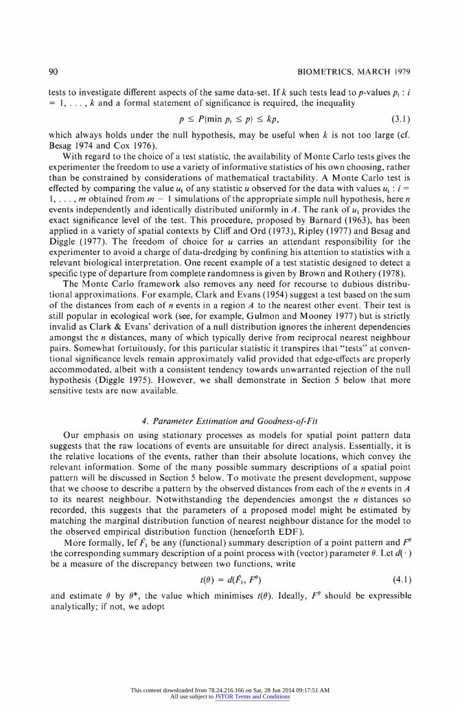
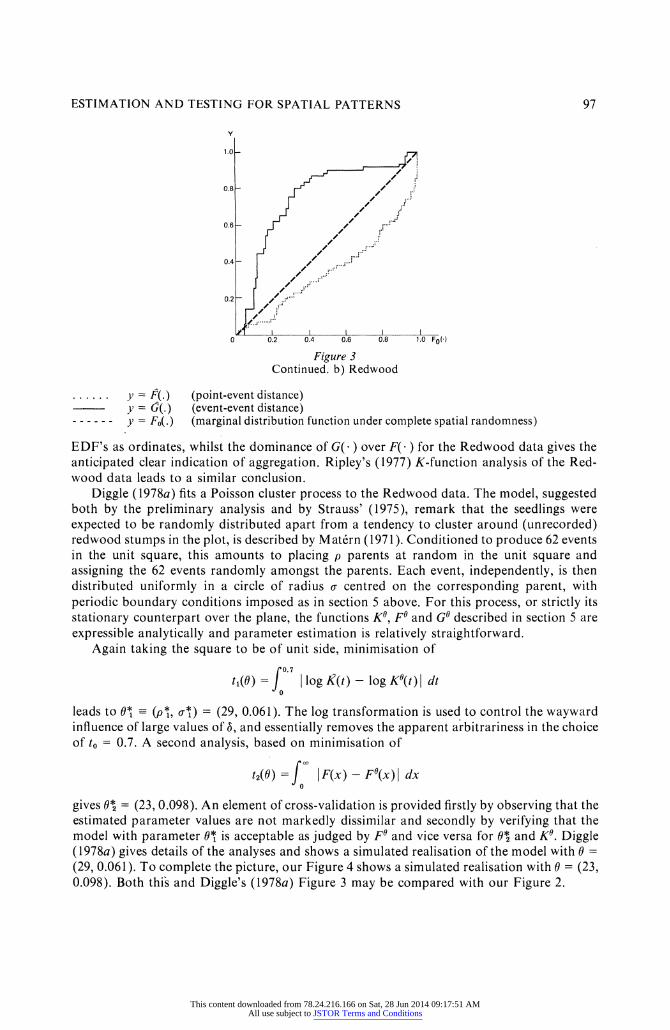
The functional nearest neighbour statistics dx dy and d2 all discriminate emphatically between the two patterns. For the Japanese black pine, all three statistics accept complcte spatial randomness, with respective p-values 0.90, 0.60 and 0.65, whilst for the Redwood all three reject with p = 0.01, incidentally the most extreme result possible from a Monte Carlo test with m - 100. Fi*gure 3 gives a graphical summary of the two analyses. The EDE plots have been linearised by using the common null distribution function as abscissa and the two

y

1 .o-

o.s- 4/.? /.r jJ

....jo H 0.6- wt

j:/;Y 04 - pv

i.''

0.2- S

, zeS

: I | I I I

0 0.2 0.4 0.6 0.8 1.0 Fo ( )

Figure 3 Empirical distribution functions of nearest neighbour distances. a) Japanese black pine.

y - Ff ) }' d( ) y = Fo( )

(point-event distance) (event-event distance) (marginal distribution function under complete spatial randomness)




0.8- / ///

0.6- / oo .E

0.4- 1 oo ..... ;

y ,, j,,,,i 0.2- 1 oo i- ' '

r, oX I l l l I

o 0.2 0.4 0.6 0.8 l.o Fof )

Figure 3 Continued. b) Redwood

.y = F( . ) (point-event distance) y = (;(.) (event-event distance)

- - - - - - y - Fo(o) (marginal distribution function under complete spatial randomness)

EDF's as ordinates, whilst the dominance of G( ) over F( ) for the Redwood data gives the anticipated clear indication of aggregation. Ripley's (1977) K-function analysis of the Red- wood data leads to a similar conclusion.

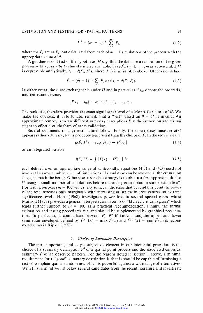
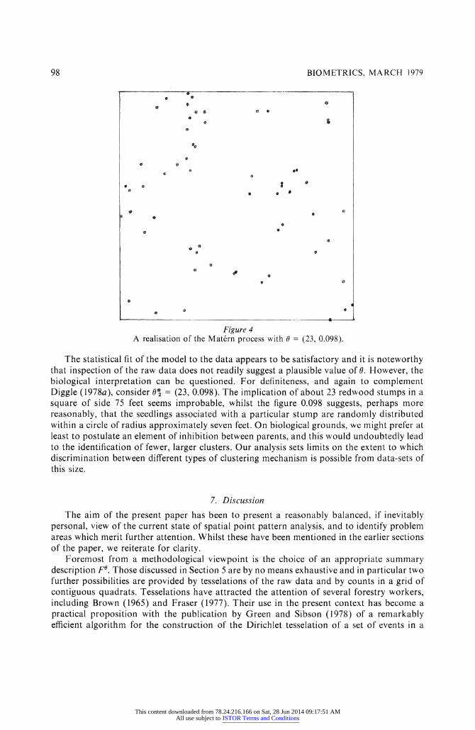
Diggle (1978a) fits a Poisson cluster process to the Redwood data. The model, suggested both by the preliminary analysis and by Strauss' (1975), remark that the seedlings were expected to be randomly distributed apart from a tendency to cluster around (unrecorded) redwood stumps in the plot, is described by M atern (1971). Conditioned to produce 62 events in the unit square, this amounts to placing p parents at random in the unit square and assigning the 62 events randomly amongst the parents. Each event, independently, is then distributed uniformly in a circle of radius ff centred on the corresponding parent, with periodic boundary conditions imposed as in section 5 above. For this process, or strictly its stationary counterpart over the plane, the functions K0, Fa and Ga described in section 5 are expressible analytically and parameter estimation is relatively straightforward.

Again taking the square to be of unit side, minimisation of ro.7

t1(0) = J | log K(t)-log K0(t) | dt o

leads to 0* - (p*, v*) = (29, 0.061). The log transformation is used to control the wayward influence of large values of 6, and essentially removes the apparent arbitrariness in the choice of to = 0.7. A second analysis, based on minimisation of

rO t2(0 ) = J | F(X )-F0(x ) | dx

o

gives 0* = (23, 0.098). An element of cross-validation is provided firstly by observing that the estimated parameter values are not markedly dissimilar and secondly by verifying that the model with parameter 0* is acceptable as judged by Fa and vice versa for 0* and K0. Diggle (1978a) gives details of the analyses and shows a simulated realisation of the model with 0 = (29, 0.061). To complete the picture, our Figure 4 shows a simulated realisation with 0 = (23, 0.098). Both this and Diggle's (1978a) Figure 3 may be compared with our Figure 2.




-

0

0 o

0 $

o e°

0 o e

o @ @

9 e o

e

o e o o

o

Gt @ e

_ _

Figure 4 A realisation of the Matern process with 0 = (23, 0.098).

The statistical fit of the model to the data appears to be satisfactory and it is noteworthy that inspection of the raw data does not readily suggest a plausible value of 0. However, the biological interpretation can be questioned. For definiteness, and again to complement Diggle (1978a), consider 0* = (23s 0.098). The implication of about 23 redwood stumps in a square of side 75 feet seems improbable, whilst the figure 0.098 suggests, perhaps more reasonably, that the seedlings associated with a particular stump are randomly distributed within a circle of radius approximately seven feet. On biological grounds, we might prefer at least to postulate an element of inhibition between parentsS and this would undoubtedly lead to the identification of fewer, larger clusters. Our analysis sets limits on the extent to which discrimination between diSerent types of clustering mechanism is possible from data-sets o

. . t llS SlZO.

7. Discussion

The aim of the present paper has been to present a reasonably balanced, if inevitably personal, view of the current state of spatial point pattern anatysisS and to identify problem areas which merit further attention. Whilst these have been mentioned in the earlier sections of the paper, we reiterate for clarity.

Foremost from a methodological viewpoint is the choice of an appropriate summary description F0. Those discussed in Section 5 are by no means exhaustive and in particular two further possibilities are provided by tesselations of the raw data and by counts in a grid of contiguous quadrats. Tesselations have attracted the attention of several forestry workers, including Brown (1965) and Fraser (1977). Their use in the present context has become a practical proposition with the publication by Green and Sibson (1978) of a remarkably efficient algorithm for the construction of the Dirichlet tesselation of a set of events in a




planar region A. This assigns to each event a convex polygonal cell consisting of those points in A closer to the event in question than to any other event. Claims made by Vlncent er al. (1976) for the eSectiveness of statistics based on the Dirichlet tesselation have yet to be assessed objectively, but undoubtedly the general approach has possibilities. Contiguous quadrat counts have a rather longer pedigree. In the present context, one possibility would be to calculate a variance-area curve analogous to the variance-time curve used to describe temporal point patterns (Cox and Lewis 1966, Chapter 4, 5, 10), and similar in spirit if not in technical detail to the popular procedure initiated by Greig-Smith (1952). We remark that there are good theoretical reasons for supposing that a variance-area curve will behave rather like a discretised version of Ripley's K-function, and might therefore have consid- erable practical merit for the analysis of very large data-sets.

A second consideration is the construction of a statistic which most effectively extracts the information from the chosen summary description. The statistics used in the present paper are intuitively reasonable, but can we do better? One possibility lies ln Besag's (1977a) construction of a pseudo-likelihood function for a Markov point process observed on a fine quadrat grid.

Spatial point processes can be studied in parallel with the development of statistical methods for point patterns. Although explicit distributional results are not strictly necessary for a simulation-based statistical methodology, the danger of any simulation study is its tendency to particularize. Theoretical results, here as elsewhere, provide for greater economy of expression. One theoretical question with obvious practical implications is the relationship of purely spatial point processes to spatial-temporal processes. Preston (1976), Kingma (1977) and Ripley (1977) give some results in this area.

Finally, a superficially practical point which also has implications of a more philosophical nature concerns the size of datasset which we envisage. In principle, larger data-sets carry more information and lead to more efficient parameter estimatesS etc. But, except ln a controlled experimental environment, each increase in the extent of data-collection necessi tates a re-assessment of the assumptions underlying any proposed model Spatial point patterns are seldom extendable at will, in the sense that some physical time-selies are.

A cknowledgments I am grateful to Richard Gratton for help with the simulation study reported in Section 5

above. The first draft of the paper was prepared during a visit to the Department of Operational Efficiency, Swedish University of Agricultural Sciences, Garpenberg, Sweden.

References

Barnard, G. A. (1963). Contribution to the discussion of Professor Bartlett's paper. Journal of the RoAal Statistical Society Series B 26, 294.

Bartlett, M. S. (1964). Spectral analysis of two-dimensional point processes. Bionletrika 44, 299 311. Bartlett, M. S. ( 1975). The Statistical Analysis of Spatial Pattern. Chapman & Hall, London. Besag, J. (1974). Spatial interaction and the statistical analysis of lattice systems (with discussion).

Journal of the Royal Statistical Society, Series B 36, 192-z236. Besag, J. (1977a). Some methods of statistical analysis for spatial data. Bulletin of the International

Statistical Institute 47. Besag, J. ( 1977b). Contribution to the discussion of Dr. Ripley's paper. Journal of the Royal Statistical

Society, Series B 39, 193-5. Besag, J. & Diggle, P. J. (1977). Simple Monte Carlo tests for spatial pattern. Applied Statistics 26, 327-

33.




Brown, G. S. (1965). Point density in stems per acre. New Zealand Forestry Service Research Notes 38, 1-11.

Brown, l[). 8c Rothery, P. (1978). Randomness and local regularity of points in a plane. Biometrika 65, 115-22. Clark, P. J. & Evans, F. C. (1954). Distance to nearest neighbour as a measure of spatial relationships in populations. Ecology 35, 23-30. CliS9 A. D. & Ord, J. K. (1973). Spatial Atltocorrelation. Pion, London. Cox, D. R. (1955). Some statistical methods connected with series of events. Journal of the Royal Statistical Society, Series B 17, 129-64. Cox, D. R. (1976). The role of significance tests. Scandinavian Journal of Statistics 4, 49-70. Cox, D. R. & Lewis, P. A. W. (1966). The Statistical Analysis of Series of Events. Methuen, London. Diggle, P. J. (1975). Contribution to the discussion of Drs. CliS & Ord's paper. Journal of the Royal Statistical Society, Series B 3 7, 333-4. Diggle, P. J. (1978a). On parameter estimation for spatial point processes. Journal of the Royal Statistical Society, Series B 40, 178-81. Diggle, P. S. (1978b). Statistical methods for spatial point patterns in ecology. International Statistical Ecology Program Proceedings (to appear). Diggle, P. J., Besag, J. & Gleaves, J. T. (1976). Statistical analysis of spatial point patterns by means of

distance methods. Biometrics 32, 659-67. Fisher, R. A., Thornton, H. G. & Mackenzie, W. A. (1922). The accuracy of the plating method of

estimating the density of bacterial populations, with particular reference to the use of Thornton's agar medium with soil samples. Annals of Applied Botany 9, 325-59. Fraser, A. R. (1977). Triangle based probability polygons for forest sampling. Forest Science 23, 111- 21. Green, P. J. & Sibson, R. (1978). Computing Dirichlet tesselations in the planc. The Computer Journal 21, 168-73. Greig-Smith, P. (1952). The use of random and continuous quadrats in the study of the structure of plant communities. A nnals of Botany 16, 293-316. Greig-Smith, P. (1964). Quantitative Plant Ecology (2nd ed.). Butterworth, London. Gulmon, S. L. & Mooney, H. A. (1977). Spatial and temporal relationships between two desert shrubs, atriplex hyss1onelytra and tidestromia oblongifolia in Death Valley, California. Journal of Ecology 65, 831-8. FIolgate, P. (1965). Tests of randomness based on distance methods. Biometrika 52, 345-53. Hope, A. C. A. (1968). A simplified Monte Carlo significance test procedure. Journal of the Royal Statistical Society, Series B 30, 582-98. Kingman, J. F. C. (1977). Remarks on the spatial distribution of a reproducing population. Journal of A pplied Prohahility 14, 577-83. Kooijman, S. A. L. M. (1977). Unpublished Ph.D. Thesis, University of Leiden, Holland. Alarriott, F. H.C.(1979). Barnard'sMonteCarlotests: howmanysimulations? AppliedStatistics28. Matern, B. (1960). Spatial Variation Reports of the Forest Research Institute of Sweden, Bd.49, No. 5

Stockholm. Matern, B. (1971). Doubly stochastic Poisson processes in the plane. ln Statistical Ecology, Vol. l, ed. G. P. Patil, E. C. Pielou, W. E. Waters, 195-213. Pennsylvania State University Press, University Park, Pennsylvania. NIead, R. (1974). A test for spatial pattern at several scales using data from a grid of contiguous

quadrats. Biometrics 30, 295-307. Miles, R. E. (1970). On the homogeneous planar Poisson point process. Mathematical Bioscies1ces 6, 85-127. Neyman, J. (1939). On a new class of contagious distributions, applicable in entomology and bacte- riology. Al nnals of IFfathematical Statistics lO, 35-57. INeyman, J. & Scott, E. L. (1958). Statistical approach to problems of cosmology. Journal of the Royal Statistical Sociery, Series B 20, 1-43. N umata, M. (1961). Forest vegetation in the vicinity of Choshi. Coastal flora and vegetation at Choshi,

Chiba Prefecture IV (in Japanese). Bulletin of the Choshi Marine Laboratory No. 3, 28-48, Chiba U niversity. Paloheimo, J. E. (1971). On a theory of search. Biometrika 58, 61-75. Preston, C. J. (1976). Spatial birth-and-death processes. Bulletin of the International Statistical Institute 46



ESTI MATION AND TESTING FOR SPATIAL PATTERNS 101

Ripley, B. D. (1977). Modelling spatial patterns (with Discussion). Journal of the Royal Statistical Society, Series B 39, 172-212.

Ripley, B. D. & Kelly, F. P. (1977). Markov point processes. Journal of the Lorldon Mathematical Society 15, 188-92

Silverman, B. W. (1978). Distances on circles, toruses and spheres. Journal of Applied Probability 15, 136-43.

Strauss, D. J. (1975). A model for clustering. Biometrika 62, 467-75. Vincent, P. J., Haworth, J. M., Griffiths, J. G. & Collins, R. (1976). The detection of randomness in

plant patterns. Journal of Biogeography 3, 373-80.



perspectives in biometry || on parameter estimation and goodness-of-fit testing for spatial point...

Documents