Research Collection

Report

Automatic problem-specific hyperparameter optimization andmodel selection for supervised machine learning: TechnicalReportTechnical Report

Author(s): Bermúdez-Chacón, Róger; Gonnet, Gaston H.; Smith, Kevin

Publication Date: 2015

Permanent Link: https://doi.org/10.3929/ethz-a-010558061

Rights / License: In Copyright - Non-Commercial Use Permitted

This page was generated automatically upon download from the ETH Zurich Research Collection. For moreinformation please consult the Terms of use.

ETH Library

Automatic problem-specific hyperparameteroptimization and model selection for supervised

machine learning

Technical Report

Róger Bermúdez-Chacón, Gaston H. Gonnet, and Kevin Smith

ETH Zurich

Zurich, 2015

Abstract

The use of machine learning techniques has become increasingly widespread in commercial

applications and academic research. Machine learning algorithms learn a model from data

that allows computers to make and improve predictions or behaviors. Despite their popularity

and usefulness, most machine learning techniques require expert knowledge to guide the

decisions about the most appropriate model and settings for a particular problem. In many

cases, expert knowledge is not readily available. When it is, the complexity of the problem

and subjectivity of the expert can often lead to sub-optimal choices in the machine learning

strategy.

Since different machine learning techniques are suitable for different problems, choosing the

right technique and fine-tuning its particular settings are crucial tasks that will directly impact

the quality of the predictions. However, deciding which machine learning technique is most

well suited for processing specific data is not an easy task, as the number of choices is usually

very large.

In this work, we present a method that automatically selects the best machine learning

algorithm for a particular set of data, and optimizes its parameter settings. Our approach

is flexible and customizable, enabling the user to specify their needs in terms of predictive

power, sensitivity, specificity, consistency of the predictions, and speed, among other criteria.

The results obtained show that using the machine learning technique and configuration sug-

gested by our automated approach yields predictions of a much higher quality than selecting

the technique with the best results under its default settings. We also present a method to

efficiently guide the search for optimal parameter settings by identifying ranges of values for

each setting that produce good results for most problems. By transferring this knowledge to

new problems, it is possible to find the optimal configuration of the algorithm more quickly.

Keywords: Model selection, hyperparameter optimization, Supervised Machine Learning

iii

Contents

Abstract iii

List of figures vi

List of tables vii

1 Introduction 1

2 Problem description 5

2.1 Formal definition . . . . . . . . . . . . . . . . . . . . . . . . . . . . . . . . . . . . . 5

2.2 Related work . . . . . . . . . . . . . . . . . . . . . . . . . . . . . . . . . . . . . . . . 7

3 Methodology 9

3.1 Hyperparameter space modeling . . . . . . . . . . . . . . . . . . . . . . . . . . . . 10

3.1.1 Hyperparameter distributions . . . . . . . . . . . . . . . . . . . . . . . . . 10

3.1.2 Hyperparameter hierarchy . . . . . . . . . . . . . . . . . . . . . . . . . . . 12

3.1.3 Sampling the hyperparameter space . . . . . . . . . . . . . . . . . . . . . . 14

3.2 Model performance measurement . . . . . . . . . . . . . . . . . . . . . . . . . . . 15

3.3 Model validation . . . . . . . . . . . . . . . . . . . . . . . . . . . . . . . . . . . . . 17

3.4 Optimization . . . . . . . . . . . . . . . . . . . . . . . . . . . . . . . . . . . . . . . 18

3.4.1 Random search . . . . . . . . . . . . . . . . . . . . . . . . . . . . . . . . . . 18

3.4.2 Shrinking hypercube . . . . . . . . . . . . . . . . . . . . . . . . . . . . . . . 19

3.4.3 Parametric density optimization . . . . . . . . . . . . . . . . . . . . . . . . 20

3.5 Model evaluation and selection . . . . . . . . . . . . . . . . . . . . . . . . . . . . . 20

3.5.1 Candidate model filtering . . . . . . . . . . . . . . . . . . . . . . . . . . . . 20

3.5.2 Statistical analysis . . . . . . . . . . . . . . . . . . . . . . . . . . . . . . . . 21

3.5.3 Ranking criteria . . . . . . . . . . . . . . . . . . . . . . . . . . . . . . . . . . 23

3.5.4 The model selection algorithm . . . . . . . . . . . . . . . . . . . . . . . . . 24

3.6 Implementation details . . . . . . . . . . . . . . . . . . . . . . . . . . . . . . . . . 24

4 Hyperparameter distribution learning 27

4.1 Learning the general prior distribution . . . . . . . . . . . . . . . . . . . . . . . . 28

4.2 Using the general prior for hyperparameter optimization . . . . . . . . . . . . . 30

v

Contents

5 Evaluation of results 31

5.1 Results on standard Machine Learning datasets . . . . . . . . . . . . . . . . . . . 32

5.2 Results on biological data . . . . . . . . . . . . . . . . . . . . . . . . . . . . . . . . 33

5.3 General prior learning . . . . . . . . . . . . . . . . . . . . . . . . . . . . . . . . . . 33

6 Conclusion 37

6.1 Future work . . . . . . . . . . . . . . . . . . . . . . . . . . . . . . . . . . . . . . . . 37

A Supervised machine learning algorithms 39

B Datasets 41

vi

List of Figures

1.1 Decision boundaries for several different SML algorithms . . . . . . . . . . . . . 2

3.1 General methodology diagram . . . . . . . . . . . . . . . . . . . . . . . . . . . . . 9

3.2 Distributions used to model hyperparameters . . . . . . . . . . . . . . . . . . . . 11

3.3 Hyperparameter hierarchy example . . . . . . . . . . . . . . . . . . . . . . . . . . 14

3.4 Hierarchical model selection . . . . . . . . . . . . . . . . . . . . . . . . . . . . . . 21

5.1 Optimized vs default values for a standard machine learning dataset . . . . . . 34

5.2 Optimized vs default values for biological datasets of different sizes . . . . . . . 35

5.3 Learned general priors . . . . . . . . . . . . . . . . . . . . . . . . . . . . . . . . . . 36

vii

List of Tables

3.1 Components of the Performance Index . . . . . . . . . . . . . . . . . . . . . . . . 16

3.2 Alternative model ranking criteria . . . . . . . . . . . . . . . . . . . . . . . . . . . 23

5.1 Comparison of optimized and default performance indices for all datasets. . . 32

ix

CHAPTER 1Introduction

Automatic data processing and analysis is essential in many scientific disciplines and com-

mercial applications. The ever-increasing availability of computational resources experienced

in recent years has stimulated the establishment of new disciplines that strongly depend

on analysis of massive amounts of data. The complexity and scale of the data means that

analysis by hand is often impractical or even impossible. Therefore automatic processing by

computational methods are of paramount importance.

A clear example of this is found in biology. Methods to automate data acquisition have

given rise to powerful new techniques such as genome-wide association studies, high-content

screening, and gene expression profiling. These techniques collect vast amounts of data that

must be carefully analyzed – a task which would have been impossible to do by hand, just a

few years ago.

Recently, machine learning has become an essential step in the analysis process of many such

techniques. Machine learning is a popular approach to automatic data processing and pattern

recognition that learns a predictive model from example data. Later, the predictive model can

be applied to new data for recognition or to make predictions. It is now common practice to

use machine learning to perform the analysis of many biological data sets because it is faster,

more accurate, and less biased than manual analysis.

Machine learning methods can be broadly categorized as either supervised or unsupervised.

Supervised methods are more widely used. They infer a predictive model by detecting pat-

terns in a set of labeled example data provided to the algorithm. Unsupervised methods are

designed to work without any training information. Clustering methods are a typical example

of unsupervised learning.

In this work, we focus on supervised machine learning (SML) methods, which are designed to

address two families of problems: classification and regression. In the classification problem,

instances of data (or objects) are said to belong to one class from a given set of classes. The

task is to assign unseen instances to the appropriate class. The regression problem attempts

to fit a model to observed data in order to quantify the relationship between two groups of

1

Chapter 1. Introduction

The two moonclassification problem.

k-nearest neighbors(k = 3) 99.6%

Adaboostwith circular areas 100%

SVM3r d order polynomial 91.5%

Neural network(1 layer, 6 nodes) 96.1%

SVMradial basis function 100%

Figure 1.1: Decision boundaries for several different supervised machine learning algorithms applied to the twomoon dataset. Inherent differences among the various models are reflected in their performance and by the shapeof the decision boundaries.

variables, predictors and responses. The fitted model can be used to describe the relationship

between the two groups, or to predict new response values based on the predictor values.

Model selection

Although many SML methods exist, it is usually not obvious which one to use. Choosing the

best algorithm for a particular problem can be difficult, even for an expert. There are several

reasons for this. First, the models underlying various machine learning algorithms are very

different from one another. In a simple example using toy data depicted in Figure 1.1, the

differences among various machine learning methods are obvious. Some methods misclassify

entire regions of the data, some perform well but generalize poorly (they overfit the data), and

for some the decision boundary is not smooth leading to ambiguity in certain regions.

Unfortunately, there is no “silver bullet” machine learning algorithm that always performs

well. The choice of the method to use is tied to the structure of the data that they are to predict.

Some methods make assumptions on the structure of the data, and do not give accurate

predictions when such assumptions are violated. Therefore, it is important to choose the most

appropriate model for the data, otherwise performance will suffer.

Hyperparameter optimization

Hyperparameters present a further complication to the problem. Most machine learning

algorithms contain hyperparameters, external settings left to be tuned by the user (as opposed

to parameters, which are optimized internally within the algorithm). These hyperparameter

2

settings, such as the cost of a support vector machine (SVM) or the number of neighbors k in

k-nearest neighbors (KNN), control the SMLs internal behavior and can affect its ability to

learn patterns for prediction. Finding the right combination of values may be as critical to

good prediction as selecting the right machine learning method.

The space of possible hyperparameters can be quite large. One common implementation of

an SVM requires the user to choose among 64 distinct categories of models, and then to set

between 2 to 4 numeric values for each category. In many cases, an exhaustive evaluation of

all possible hyperparameter combinations is not practical, and it is often not even possible. In

practice, hyperparameter tuning is more of an art than a science, and even machine learning

experts often carry out the tuning in an arbitrary or subjective way.

Our approach

We present an automatic solution to the combined model selection and hyperparameter

optimization problem. Model selection is the problem of determining which among a set

of machine learning algorithms is the most well suited to the data, while hyperparameter

optimization searches for candidate hyperparameter values expected to most improve the

prediction of the SML algorithm.

Our approach is to organize the various machine learning algorithms and their hyperparam-

eters into a large hierarchical space. At the lowest level of the hierarchy are the numeric

hyperparameters which contain values that must be set appropriately. Up the hierarchy we

model conditional and categorical choices, which all belong to a single family of machine

learning algorithms (support vector machines, for example). We use numeric optimization

methods at the lowest level to choose the best numeric hyperparameter values for a given

categorical configuration. The candidate models compete against each other using statistical

tests. The best candidates are promoted to the next level of the hierarchy. The process is

repeated until ultimately a single model remains, chosen among the families of classifiers or

regressors.

Our approach substantially improves the performance of machine learning algorithms over

their default settings, as we demonstrate on classic machine learning datasets as well as

biological data. Our analysis also recognizes that, in some cases, the difference between one

or more candidate models is statistically insignificant. When this occurs, the user can specify

alternative criteria to choose the best model such as ranking the model’s speed, simplicity, or

interpretability.

3

CHAPTER 2Problem description

This work aims to propose a solution for a two-fold problem: find the SML algorithm that

works best for a given set of data, and find which particular choice of configuration settings

for that algorithm yields the best results.

Although both sides of the problem correspond conceptually to different ideas (general ap-

proach the former, fine-tunning the latter), they are intrinsically linked and should not be

treated as separate problems. This is especially true for the present work, since a poor choice

of settings for an otherwise well-suited SML algorithm may be easily outperformed by another,

less appropriated SML method, applied on the same data.

The formal description of the problem presented here is given in terms of the classification

problem, but this description extends naturally to the regression problem.

2.1 Formal definition

The following terms and notation will be used for the rest of this document:

• An instance is data representing a single example, often an object. It is encoded as a pair

(x, y), with x a vector of values for attributes (also called features) related to the object,

and y a mapping of the object to its corresponding class.

• A dataset D = {(x1, y1), (x2, y2), . . . , (xN , yN )} is a set of instances on which SML is to be

applied.

• An algorithm A is a specific implementation of any function that uses known in-

stances (x, y) (also known as examples) to learn patterns or rules to associate the feature

values x to their class y , and uses this information to predict the class y ′ of unseen

instances from their feature values x′.

A : ({(x, y)}, {x′}) 7→ {y ′} (2.1)

5

Chapter 2. Problem description

• A= {A1, . . . , Ak } represents the set of all algorithms to evaluate.

• An algorithm A accepts a set of hyperparameters PA that modify its behavior.

• λa is the value of a hyperparameter a ∈PA for some algorithm A.

• λi = (λia ,λi

b ,λic , . . .) denotes a set of hyperparameter values (or configuration) for the

i -th algorithm in A.

• Λi represents the set of all possible values that λi can take (i.e. the hyperparame-

ter space of the i -th algorithm).

• A realization of algorithm A under a specific configuration λ is called a model, and

represented as Aλ.

• The scoring function S measures the predictive performance of a model Aλ on unseen

instances drawn from the dataset D.

S : Ai ∈A,λi ∈Λi ,D 7→R (2.2)

The scoring function should be designed in such a way that the better the agreement

between class prediction and true class assignment is, the higher the score.

It is assumed that the feature values of the examples x used for training an algorithm and the

feature values to predict labeling x′ are drawn from the same underlying distribution, and that

instances with similar feature values tend to belong to the same class.

Under the described context, the model selection and hyperparameter optimization problem

can be defined as:

A∗λ∗ = argmax

Ai∈A,λi∈Λi

S(Aiλi ,D) (2.3)

The above equation can be simply stated as "find the algorithm and its parameter values that

obtain the best score at predicting labels on the given dataset". It is worth noticing that equa-

tion 2.3 is the general form of the optimization process, and as such, only defines the structure

and general behavior of the different components of the optimization. In practice, additional

details such as the implementation of the scoring function, and the actual exploration of the

hyperparameter spaces, must be considered.

Furthermore, the assumption that a single model A∗λ∗ will be significantly better than the

rest is not guaranteed, and hence returning multiple models as the result of the optimization

process should also be considered under certain circumstances.

6

2.2. Related work

2.2 Related work

Few initiatives to address the model selection and hyperparameter optimization of SML

algorithms have been proposed.

For hyperparameter optimization, the de facto method, known as grid search, is the exhaustive

evaluation of a discretization of the hyperparameter space on a regularly-spaced grid. This

approach is affected by the curse of dimensionality when a large number of hyperparameters

needs to be analyzed. Furthermore, the step size for discretization is often decided arbitrarily.

Alternative methods to avoid these shortcomings have been proposed. The simplest of all

consists on randomly retrieving and evaluating values for the hyperparameters (random

search), and is studied in the context of SML optimization in [?]. This method is obviously

very slow as it relies only on chance to find good configurations. It does, however, allow for a

uniform exploration of the hyperparameter space.

A method based on hierarchical density estimation, and another method based on hierarchi-

cal Gaussian processes, are proposed in [?]. These methods are limited to the optimization

of hyperparameter values from a single SML algorithm, and do not consider a systematic

selection of a model. Furthermore, the work lacks a statistical analysis of the optimized hyper-

parameters, and does not properly consider the generalization of the selected configuration

to unseen data.

The very recent approach implemented in Auto-WEKA ([?]) does consider model selection

and hyperparameter optimization simultaneosly. Their work models the hyperparameter

space in a hierarchical way. Auto-WEKA considers generalization as the only criterion for both

optimization and model selection.

Statistical frameworks for model selection on SML are described in [?] and [?], and some of

their ideas have been implemented in the present work.

7

CHAPTER 3Methodology

The specific implemented approach to find solutions for equation 2.3 is explained in detail in

this chapter. Important components of the solution described here include the modeling of

the hyperparameter space, how to sample from the hyperparameter space, the choice of the

numerical optimization method, and the definition of the target function to optimize, among

others.

The general strategy followed here is summarized in figure 3.1:

optimizer

evaluate

Promising configurations

λ1λ2λ3λ4

λn

validation

evaluate

…

…

D

S H

S(A, λ1),…

S(A, λ)A, λ,S

A, λ λ1,…,λn

A, λ,H S(A, λ)

candidates

optimization

model selectionh1

…

…

S(A, λ1),S(A, λ2),…

model selectionh2

…

…

…

…

A, λ*

A, λ*

Aλ*

Figure 3.1: Interaction between different components of the implemented hyperparameter optimization andmodel selection approach.

The entire process is divided in two stages. The instances contained in the dataset D are

divided into two subsets S and H. The hyperparameter optimization stage explores and

9

Chapter 3. Methodology

evaluates a large number of models (SML algorithm under a given configuration) on the subset

S , in order to find the ones that exhibit the best predictive performance. The model selection

stage analyzes the most promising models obtained from the hyperparameter optimization

stage (candidates) under the subset H (data unseen to the optimization process). To assess

generalization, it uses that information, along with other desirable properties of the models,

to systematically rule out suboptimal models and finally return the best.

3.1 Hyperparameter space modeling

Most SML algorithms contain configuration options that control different aspects of their

internal behavior, which can be further adjusted to fit specific needs. For example, algorithms

that make use of the distance between examples in feature space might accept a distance

metric to be specified, or algorithms that internally create trees might allow the user to specify a

branching factor (maximum number of branches per node), and so on. Since the configuration

options control the behavior of the algorithm, they are regarded to as hyperparameters of the

SML algorithm. The choice of hyperparameter values for a SML algorithm can heavily impact

its predictive power.

Different types of hyperparameters exist. Nominal hyperparameters take values from a fixed

list of categories that usually correspond to a decision of how the SML algorithm performs

the predictions. Such categorical hyperparameters include, for instance, which kernel to use

to compute support vectors in a support vector machine classifier, or whether to consider

the distance between neighboring points or not on the prediction of a k-nearest neighbors

classifier. Once all these decisions have been made, numerical hyperparameters control the

values to use for the specific implementation of internal formulas needed for prediction, such

as the number of neighbors for k-neighbors classification, or the cost parameter used by a

support vector machine as a trade-off between allowing training errors and rigidly fitting the

support vectors to the training set.

Other considerations such as restricting the value of a numerical hyperparameter to a fixed

range (addressed here by assigning validation rules for each numerical hyperparameter), or

encoding dependencies between categorical and numerical or other categorical hyperparam-

eters (implemented here as explained in detail in subsection 3.1.2) must be taken into account

when modeling the strategy to explore the hyperparameters of a SML algorithm.

3.1.1 Hyperparameter distributions

Since one of the main objectives of this work is to learn the behavior of SML algorithms

under different settings, a systematic way of obtaining valid candidate configurations for

performance evaluation is required. In order to achieve this, each hyperparameter is regarded

as a random variable and an appropriate distribution modeling the likelihood of obtaining

good performance for a given value is assigned to it.

10

3.1. Hyperparameter space modeling

Uniform

a b

Normal

µ

Categorical

p(x

)

λ1

λ2

λ3

Log−uniform

a b

Log−normal

µ

Gaussian Mixture

µ1

µ2

µ3

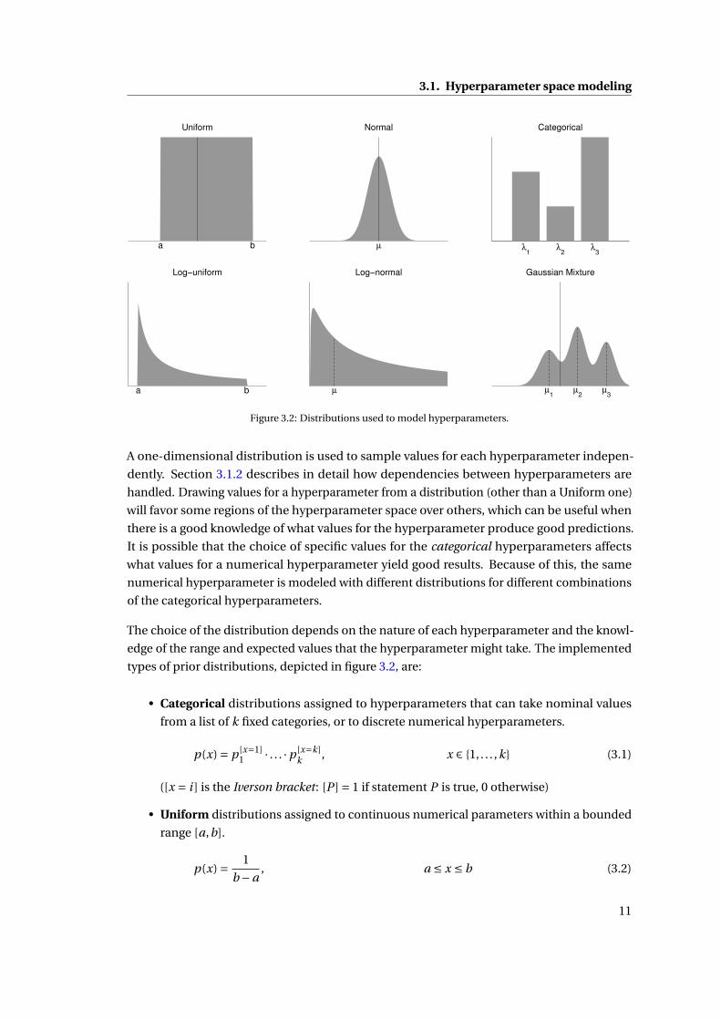
Figure 3.2: Distributions used to model hyperparameters.

A one-dimensional distribution is used to sample values for each hyperparameter indepen-

dently. Section 3.1.2 describes in detail how dependencies between hyperparameters are

handled. Drawing values for a hyperparameter from a distribution (other than a Uniform one)

will favor some regions of the hyperparameter space over others, which can be useful when

there is a good knowledge of what values for the hyperparameter produce good predictions.

It is possible that the choice of specific values for the categorical hyperparameters affects

what values for a numerical hyperparameter yield good results. Because of this, the same

numerical hyperparameter is modeled with different distributions for different combinations

of the categorical hyperparameters.

The choice of the distribution depends on the nature of each hyperparameter and the knowl-

edge of the range and expected values that the hyperparameter might take. The implemented

types of prior distributions, depicted in figure 3.2, are:

• Categorical distributions assigned to hyperparameters that can take nominal values

from a list of k fixed categories, or to discrete numerical hyperparameters.

p(x) = p [x=1]1 · . . . ·p [x=k]

k , x ∈ {1, . . . ,k} (3.1)

([x = i ] is the Iverson bracket: [P ] = 1 if statement P is true, 0 otherwise)

• Uniform distributions assigned to continuous numerical parameters within a bounded

range [a,b].

p(x) = 1

b −a, a ≤ x ≤ b (3.2)

11

Chapter 3. Methodology

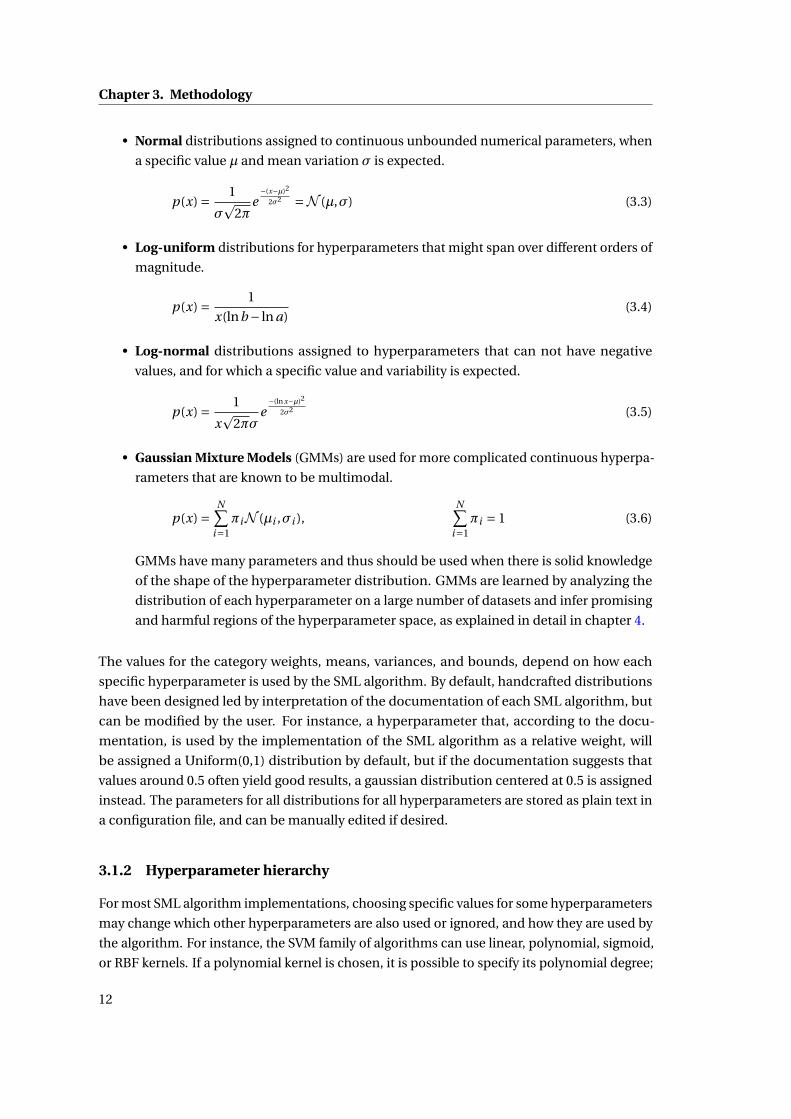
• Normal distributions assigned to continuous unbounded numerical parameters, when

a specific value µ and mean variation σ is expected.

p(x) = 1

σp

2πe

−(x−µ)2

2σ2 =N (µ,σ) (3.3)

• Log-uniform distributions for hyperparameters that might span over different orders of

magnitude.

p(x) = 1

x(lnb − ln a)(3.4)

• Log-normal distributions assigned to hyperparameters that can not have negative

values, and for which a specific value and variability is expected.

p(x) = 1

xp

2πσe

−(ln x−µ)2

2σ2 (3.5)

• Gaussian Mixture Models (GMMs) are used for more complicated continuous hyperpa-

rameters that are known to be multimodal.

p(x) =N∑

i=1πiN (µi ,σi ),

N∑i=1

πi = 1 (3.6)

GMMs have many parameters and thus should be used when there is solid knowledge

of the shape of the hyperparameter distribution. GMMs are learned by analyzing the

distribution of each hyperparameter on a large number of datasets and infer promising

and harmful regions of the hyperparameter space, as explained in detail in chapter 4.

The values for the category weights, means, variances, and bounds, depend on how each

specific hyperparameter is used by the SML algorithm. By default, handcrafted distributions

have been designed led by interpretation of the documentation of each SML algorithm, but

can be modified by the user. For instance, a hyperparameter that, according to the docu-

mentation, is used by the implementation of the SML algorithm as a relative weight, will

be assigned a Uniform(0,1) distribution by default, but if the documentation suggests that

values around 0.5 often yield good results, a gaussian distribution centered at 0.5 is assigned

instead. The parameters for all distributions for all hyperparameters are stored as plain text in

a configuration file, and can be manually edited if desired.

3.1.2 Hyperparameter hierarchy

For most SML algorithm implementations, choosing specific values for some hyperparameters

may change which other hyperparameters are also used or ignored, and how they are used by

the algorithm. For instance, the SVM family of algorithms can use linear, polynomial, sigmoid,

or RBF kernels. If a polynomial kernel is chosen, it is possible to specify its polynomial degree;

12

3.1. Hyperparameter space modeling

such option has no effect when a linear kernel is used. Likewise, it is possible to specify the

independent term for the polynomial and sigmoid functions used as kernels, and such value

may have a different impact and different extrema depending on which kernel they operate

on. The popular SVM implementation libSVM accepts a single hyperparameter coef0 for this

setting. Disregarding the duality of this hyperparameter and its dependence on the context

(selected kernel in this case) when modeling and optimizing it might lead to unwanted results.

What the above example implies is that it is mandatory to consider each hyperparameter for

optimization within a context given by the values of other hyperparameters (the hyperparam-

eter context). We have chosen a hierarchical design, based on two observations:

1. Hyperparameter contexts can be nested. The use and semantics of a hyperparameter

may depend on the value of other hyperparameters, which may in turn depend on

others.

2. The hyperparameter context is always defined by a set of categorical, rather than numer-

ical, hyperparameters. Since the decision of whether or not to use a hyperparameter is

a discrete (boolean) value, it does not make sense to consider continuous numerical

variables when defining a hyperparameter context.

A specific situation where observation 2 may be violated is when a numerical hyperparameter

depends on a rule applied on another numerical hyperparameter, rather than on its actual

value. For example, if hyperparameter b is only used by the SML algorithm when hyperparam-

eter a adopts values within a given interval, and invalid otherwise. A virtual hyperparameter

b_valid with such rule (which would be a categorical hyperparameter with categories {True,

False}) can be added to the hyperparameter hierarchy. Hyperparameter b would exist in the

hyperparameter context given by b_valid=True and would not exist in the hyperparameter

context given by b_valid=False. Virtual hyperparameters are used only to guide the hierarchi-

cal hyperparameter sampling and validation, and should be removed from the configuration

before passing it to the SML algorithm.

Following these observations, it is possible to encode the entire hyperparameter space for a

SML algorithm into a tree structure that models the hierarchical dependences between sets

of hyperparameters. The top nodes of the tree refer to categorical hyperparameters that do

not depend on the values of others, and each category creates a new hyperparameter context

(branch) under which its depending categorical hyperparameters will be represented.

The leaves of the tree correspond to the numerical hyperparameters that are valid for the

deepest branching to which they belong. The branching of categorical hyperparameters

corresponds to a series of decisions on what values the categorical hyperparameters take, and

is refered to as the signature of the numerical hyperparameter context. Figure 3.3 provides an

example of a hyperparameter hierarchy.

The whole model selection process can be viewed as the top level of the hyperparameter

13

Chapter 3. Methodology

DecisionTreeClassifier

criterion

Gini

max_features_use_preset

False

mfs

msd md

msl

True

max_features_preset

sqrt

msd md

msl

log2

msd md

msl

None

msd md

msl

Entropy

max_features_use_preset

False

mfs

msd md

msl

True

max_features_preset

sqrt

msd md

msl

log2

msd md

msl

None

msd md

msl

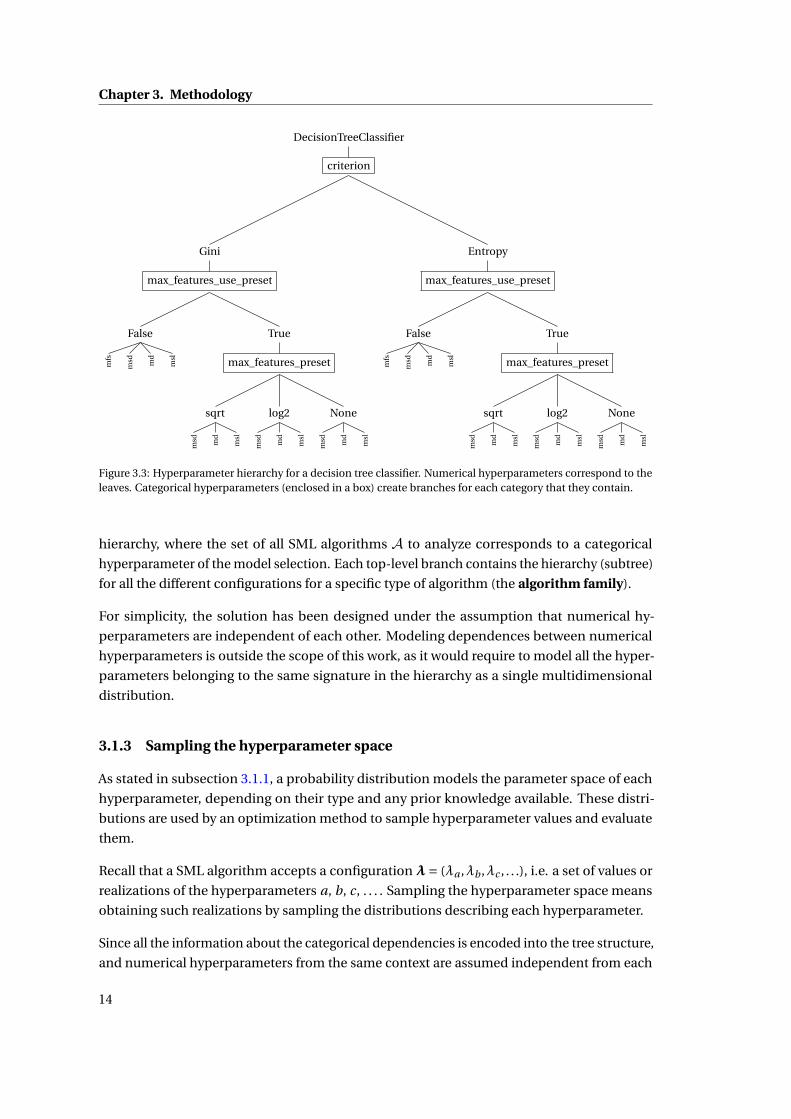
Figure 3.3: Hyperparameter hierarchy for a decision tree classifier. Numerical hyperparameters correspond to theleaves. Categorical hyperparameters (enclosed in a box) create branches for each category that they contain.

hierarchy, where the set of all SML algorithms A to analyze corresponds to a categorical

hyperparameter of the model selection. Each top-level branch contains the hierarchy (subtree)

for all the different configurations for a specific type of algorithm (the algorithm family).

For simplicity, the solution has been designed under the assumption that numerical hy-

perparameters are independent of each other. Modeling dependences between numerical

hyperparameters is outside the scope of this work, as it would require to model all the hyper-

parameters belonging to the same signature in the hierarchy as a single multidimensional

distribution.

3.1.3 Sampling the hyperparameter space

As stated in subsection 3.1.1, a probability distribution models the parameter space of each

hyperparameter, depending on their type and any prior knowledge available. These distri-

butions are used by an optimization method to sample hyperparameter values and evaluate

them.

Recall that a SML algorithm accepts a configurationλ= (λa ,λb ,λc , . . .), i.e. a set of values or

realizations of the hyperparameters a, b, c, . . . . Sampling the hyperparameter space means

obtaining such realizations by sampling the distributions describing each hyperparameter.

Since all the information about the categorical dependencies is encoded into the tree structure,

and numerical hyperparameters from the same context are assumed independent from each

14

3.2. Model performance measurement

other, each numerical hyperparameter is sampled independently.

Generating valid samples of the hyperparameter space of a SML algorithm reduces then to

getting a valid signature (by recursively sampling the distributions of the categorical hyper-

parameters in the tree) and sampling each numerical hyperparameter in the context given

by the signature independiently. The SML algorithm under the configuration resulting from

joining all these values together is the model to be evaluated over the data.

3.2 Model performance measurement

Once the strategy for generating models for evaluation has been established, the definition of

a model performance metric is required. To measure the performance of a model means to

quantify how well the prediction of it on unseen data is, and hence the quality of the labeling

obtained on the prediction step of the model is the criterion to be measured.

Because the performance measurements between different algorithms must be comparable,

a method that is agnostic to the algorithm should be defined. The labeling returned by the

prediction step of the model can be either a single class for each instance in the prediction set,

or, for some classification algorithms, a vector describing the probabilities for each instance

to be assigned to a specific class.

Predictions consisting of specific classes are transformed into probability vectors with a value

of 1 for the position corresponding to the assigned class, and 0 elsewhere. This step provides a

consistent representation for the output of all classification algorithms. For regression, the

single (possibly multidimensional) predicted value is used without further transformation.

Many metrics comparing the expected and the predicted classes exist, and different metrics

allow for evaluation of different properties of the prediction. Table 3.1 summarizes some of

the most widely used.

The output of these various metrics may take different ranges of values, and the interpretation

of the actual values might also differ from metric to metric. As an example, the accuracy of

a prediction is measured in the range between 0 and 1, and a greater value means a better

prediction. The mean squared error is measured as a positive value, and a lower value means

a better prediction in this case. In order to homogenize the metrics, upper and lower bounds

are defined for each metric, and the relative position of the original value with respect to the

bounded interval is used instead of the original value.

The upper bound is straightforward to specify, as all metrics have an ideal value that would

be achieved if the prediction agrees exactly with the true classes. To define the lower bound,

the values for each of the metrics are calculated by using a virtual prediction that assigns the

relative frequencies of each class in the dataset as the probabilities of any instance belonging

to that class (this is equivalent to weighted-randomly assigning classes to the instances). The

metrics obtained by this prediction are used as a baseline that defines the lower bound of

15

Chapter 3. Methodology

Metric Formula DescriptionAccuracy

fp+ tn

fp+ fn+ tp+ tnRatio of correctly labeled instances

Fβ score(1+β2)tp

1+β2tp+β2fn+ fpWeighted average of precision and recall. βis the relative importance of the recall withrespect to the precision

Brier score1

N

N∑t=1

R∑i=1

(pt i −ot i )2 Squared difference of probabilities returnedby the prediction pt i and true probabilitiesof the labeling ot i .

Matthews correlation coefficienttp tn− fp fn√

(tp+ fp)(tp+ fn)(tn+ fn)(tn+ fn)Balanced measure of true and false posi-tives and negatives, suitable for data havingclasses with very different frequencies.

Coefficient of determination (R2)

1−∑

i ( fi − y)2∑i (yi − y)2

Measure of fitness of the predictions to theexpected classes.

Area under ROC curve∫ ∞

−∞T PR(y)P0(y)d y Probability to obtain a better score with

a randomly chosen correctly-classified in-stance than with a randomly chosen mis-classified one.

Mean absolute error1

n

n∑i=1

| fi − yi | Absolute difference between predictions fi

and true values yi

Mean squared error1

n

n∑i=1

( fi − yi )2 Squared difference between predictions fi

and true values yi

Table 3.1: Components of the Performance Index. tp, tn, fp, and fn correspond to the true positive, true negative,false positive, and false negative count, respectively. P0 is the probability of an instance not belonging to a class.

the interval for homogenization. It is possible that some homogenized metrics lie below the

baseline, when the quality of the classification is worse than the baseline.

The selected metrics are combined into a single performance index to be used as the target

function that the optimization method will aim to maximize. The performance index S (also

referred to as the score) is defined on a set of metrics M= {m1,m2, . . . ,mz } as:

S =z∑

i=1wi mi (y, y),

z∑i=1

wi = 1 (3.7)

16

3.3. Model validation

The weights wi control the relative importance of each metric and can be tuned to suit

specific needs. For instance, if it is known that none of the SML algorithms to evaluate returns

probability estimates of the labeling, the Brier scores will coincide with the reported accuracy,

and is therefore safe to disable it by setting its weight to zero. All metrics are weighted uniformly

by default.

By default, the performance index used here combines the accuracy, the Fβ score, the Brier

score, and the Matthews correlation coefficient. These metrics have some properties that make

them suitable for a wide range of situations. The accuracy offers a very intuitive evaluation

of the quality of the prediction. The Fβ score allows for tuning of the relative importance of

the recall with respect to the precision, which might be useful depending on the needs of the

user. The Brier score takes the probability estimates into account and therefore deals with

ambiguity in the classification in a more fair way. The Matthews correlation coefficient is a

balanced metric suitable for classes with very different relative frequency.

While encoding metrics into a one-dimensional performance index may hide important

details of the individual metrics, and yields values that are not straightforward to interpret,

it is much more convenient to use it to represent the overall performance than dealing with

a multidimensional score directly. The performance index described is thus the chosen

approach for defining the optimization target function.

3.3 Model validation

Using a model validation protocol is important because it reduces the risk of overfitting a

model to the particularities of the training set, and hence is a first step to promote generaliza-

tion of the model to unseen data. The performance index calculated by equation 3.7 maps

each model to a single numerical value that represents its ability to correctly predict classes

on a specific set of training and testing instances. In order to assess the predictive quality of

the model in a more general setup, repeated rounds of stratified k-fold cross-validation are

carried out.

Each repetition corresponds to a different random shuffling of the data. The k-fold cross-

validation splits the data into k equally-sized portions (or folds), and uses one fold at a time for

prediction (and the remaining k −1 folds for training the model). Stratified cross-validation

means here that the folds are enforced to all have the same proportion of examples for each

class.

In most applications, a single repetition of 10-fold cross-validation is used, the scores obtained

for each fold are averaged out and used as a single score. This means that, for each fold, the

model is trained with 90% of the data and tested against the remaining 10%. The analysis by

Kohavi ([?]) justifies the choice of k = 10 as the smallest number of folds with "acceptable"

bias. The actual number of repetitions and folds used in this work is exposed as a parameter

that can be customized at will.

17

Chapter 3. Methodology

For the optimization stage, the standard 10-fold cross-validation is used by default. For

the model selection stage, since a more limited number of candidate configurations will be

evaluated, and because a statistical analysis is to be performed on the distribution of results,

a larger number of evaluations for each model can and should be obtained. Normality of

the distribution of scores is assumed. Performing 3 repetitions of 10-fold cross-validation is

suggested, to comply with the rule of thumb (derived from the central limit theorem) of using

a sample size of at least 30 samples to estimate a normal distribution.

3.4 Optimization

The optimization stage retrieves configurations, evaluates their performance, and uses the

performance measurements to guide the retrieval of new configurations towards regions of

the hyperparameter space expected to show predictive improvement.

Since the aim of this work is to provide the framework for hyperparameter optimization and

model selection, rather than to study different optimization techniques, only a couple of

optimization methods have been implemented. More sophisticated optimization methods

such as simulated annealing and genetic algorithms could also be used. The framework

described here assumes only that the optimization method returns candidate configurations,

and can be fed with their evaluation results in order to train itself if needed.

The optimization methods work on the numerical dimensions of the hyperparameter space

only. This is particularly convenient because most current optimization methods are not

capable of handling hierarchical, conditional and categorical spaces. Since the proposed

strategy does not impose any further restrictions or special handling of the non-numerical

dimensions, there is no need for specially designed optimization methods.

The optimization stage is restricted by a fixed time budget, shared across all the SML algo-

rithms.

3.4.1 Random search

The easiest way to generate candidate configurations is to simply draw values at random for

each hyperparameter.

The considerations stated in subsection 3.1.3 must be respected, namely the hyperparameter

sampling must start from the root of the hyperparameter hierarchy, obtain a realization

of the top-level hyperparameter (randomly in this case), and use its value to decide what

other hyperparameters to sample. The categorical and numerical values retrieved are the

components of the configuration.

Random search does not need to keep track of the evaluated model history or the retrieved

scores, since every draw of hyperparameter values is independent of all the previous ones. As

18

3.4. Optimization

a consequence, random search is a very slow and expensive optimization method. Random

search is, however, useful when a more thorough exploration of the hyperparameter space is

required, as it gives any possible configuration the same chance to be drawn.

A very important application of random search is presented in chapter 4, where it is used as

a meta-optimizer for inferring hyperparameter distributions to train a parametric density

estimation optimizer.

3.4.2 Shrinking hypercube

Unlike the random search, the shrinking hypercube method described in [?] does make use of

the scores returned by previous optimization rounds to guide the search to a local maximum.

The shrinking hypercube algorithm works by defining a region of the multidimensional pa-

rameter space for exploration, delimited by a hypercube centered about the configuration

that produces the best result of all the tested configurations. The hypercube will shrink when

no improvement is found, to localize the search, and expanded when a new best is found, to

stimulate exploration.

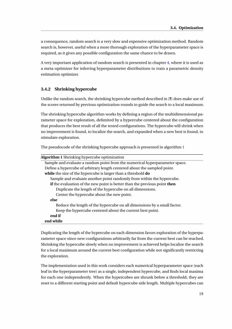
The pseudocode of the shrinking hypercube approach is presented in algorithm 1

Algorithm 1 Shrinking hypercube optimization

Sample and evaluate a random point from the numerical hyperparameter space.Define a hypercube of arbitrary length centered about the sampled point.while the size of the hypercube is larger than a threshold do

Sample and evaluate another point randomly from within the hypercube.if the evaluation of the new point is better than the previous point then

Duplicate the length of the hypercube on all dimensions.Center the hypercube about the new point.

elseReduce the length of the hypercube on all dimensions by a small factor.Keep the hypercube centered about the current best point.

end ifend while

Duplicating the length of the hypercube on each dimension favors exploration of the hyperpa-

rameter space since new configurations arbitrarily far from the current best can be reached.

Shrinking the hypercube slowly when no improvement is achieved helps localize the search

for a local maximum around the current best configuration while not significantly restricting

the exploration.

The implementation used in this work considers each numerical hyperparameter space (each

leaf in the hyperparameter tree) as a single, independent hypercube, and finds local maxima

for each one independently. When the hypercubes are shrunk below a threshold, they are

reset to a different starting point and default hypercube side length. Multiple hypercubes can

19

Chapter 3. Methodology

also be used in parallel with different starting points and side lengths for a better coverage of

the hyperparameter space.

3.4.3 Parametric density optimization

A simple optimization approach that makes use of clues about generally high and low-scoring

regions in the hyperparameter space is presented in detail in chapter 4.

The distributions for all hyperparameters are estimated automatically, by running the op-

timization process on a large set of standard datasets using random search to explore the

hyperparameter space. The results of all the datasets are used to fit Gaussian mixtures that

encode the high and low-scoring regions for each hyperparameter. The Gaussian mixtures

returned by this process will replace the default distributions that represent each hyperparam-

eter.

3.5 Model evaluation and selection

The optimization stage explores the hyperparameter space and finds candidate configurations

that return a high performance index when evaluated on the optimization data set. The

selected model will be chosen from one of such candidates according to their predictive

performances on a hold out dataset, and other desirable criteria.

A very large number of candidate configurations might be proposed by the optimization

process, and hence a strategy to efficiently discard or promote configurations must be de-

signed. The tree structure chosen to represent the hyperparameters of a SML algorithm can

be exploited to this end.

The chosen strategy analyzes the local optima found by the optimization process on the leaves

of the hyperparameter tree (which only contain numerical hyperparameters), selects the

ones that are significantly better, evaluates them and ranks them according to other desirable

properties to narrow down the model selection even further. When a handful of very good

models are selected at the numerical level, they are used to represent their branching in the

tree at the deepest categorical level, and compete with representative models of the other

categories in the exact same way. The selected models among all categories are promoted

upwards to represent the category one level higher in the hyperparameter tree. The process is

repeated until the root branching of the tree is reached, i.e., when models from different SML

algorithms are compared. A schematic of the process is shown in figure 3.4.

3.5.1 Candidate model filtering

The optimization stage will mostly retrieve models with good scores because optimization

techniques try to find local optima. As a consequence, they might end up testing a large

20

3.5. Model evaluation and selection

Figure 3.4: Hierarchical model selection. Each box plot represents the distribution of scores for a specific model.Distributions shown in black are promoted upwards to subsequently compete against models from the same localhierarchy.

number of configurations close to each optimum. This means that the distribution of hyperpa-

rameter values sampled and evaluated by the optimization stage will tend to have more density

around the different local maxima found. A clustering approach is used to remove redundant

configurations and only retrieve high-scoring configurations from different local maxima.

This avoids overrepresentation of configurations from a single hill in the score landscape and

returns a small number of configurations that represent the regions that yield good scores

more homogeneously.

We apply clustering on the evaluated configurations with the k-means algorithm to retrieve

k clusters of configurations, and choose the configuration with the highest score from each

cluster as one of the candidate configurations that will represent a specific numerical hyper-

parameter space. The number of means has been arbitrarily chosen to k = 10 by default but

can be modified via a parameter setting if needed.

3.5.2 Statistical analysis

Given a set of models, the distribution of their scores on different samples drawn from of the

hold out dataset is studied to determine which model offers enough evidence to be considered

the best one.

21

Chapter 3. Methodology

The hierarchical structure of the hyperparameter space groups models that share the same

signature together, at different levels. A statistical analysis is performed at all levels of the

hyperparameter space, starting from the configurations that differ only on their numerical

hyperparameters, and promoting good models to be compared to others at the immediately

broader level of aggregation (the category immediately above in the tree) repeatedly up to the

highest level in the hierarchy.

The aim of the statistical analysis in the context of this work is to compare the distributions of

performance indices for all candidate models with respect to the highest-scoring one, and

discard all the candidate models with strong statistical evidence that they perform worse. The

models kept are statistically indistinguishable from the best one. The overall procedure is

based on [?] and [?] for significance testing.

Each model is used for prediction on the hold out dataset several times by using m repetitions

of k-fold cross-validation (m = 3, k = 10 by default). A multiple comparison statistical test

(MCT) is applied on the distributions of m ·k scores obtained for each model.

Parametric MCTs make use of direct measurements of the data (such as the mean and vari-

ance), whereas non-parametric MCTs rely on comparisons of other properties of the data (e.g.

the ranking of the groups according to some criteria) which makes them more general and

applicable to a wider range of distributions, at the expense of statistical power [?]. Parametric

comparison tests are more statistically powerful and are thus preferred over non-parametric

alternatives. Parametric tests, however, are only valid under certain specific conditions, and

when such conditions are not met, non-parametric comparison tests must be used instead.

The MCTs determine, up to a certain probability α, whether there are significant differences

between a group of distributions or not, but do not tell the actual distributions that show

differences. A post-hoc test is required in order to find which distributions differ. Both

parametric and non-parametric post-hoc tests exist.

The chosen parametric MCT is the one-way ANOVA test [?], which is a generalization of the

t-test that corrects for accumulated errors when performing comparisons between more than

two distributions, by comparing a statistic against a F -distribution that considers the specific

number of distributions to compare as a parameter.

The one-way ANOVA test can be used when:

1. The observations for all the distributions are independent.

2. The distributions are approximately normal. This is tested by applying the Kolmogorov-

Smirnov test (K-S test, validates that a sample comes from a given distribution) on the

sample (after standardization) against a standard normal distribution N (0,1)

3. The distributions have homogeneous variances (homoscedasticity). This is tested by

applying the Bartlett’s test [?] on the different distributions of scores.

22

3.5. Model evaluation and selection

As stated above, a post-hoc test is required when the ANOVA test determines that there

are significant differences between groups of scores. The Tukey’s honest significance test

compares simultaneously all the groups of scores and informs what groups are significantly

different. The Tukey’s test is then used to find the sets of performance indices that are not

significantly different from the the highest-scoring one. Here it is assumed safe to discard

models that do not pass the Tukey’s test, and keep the rest for further analysis.

When the conditions to apply the parametric MCT are not met, the Kruskal-Wallis test is

applied instead to decide if significant differences exist, and the Nemenyi test is used as

the post-hoc test to find the actual significantly different groups in the same way as for the

parametric case.

All the statistical tests make use of a critical value to reject hypotheses with a level of certainty

α. The choice of α for model selection affects what models are deemed statistically indistin-

guishable from the best. A larger α will generally reject more models than a smaller one. Since

most of the models to compare may be very similar at the family level, it is left up to the user to

decide what α values to use, to manually control the number of significantly indistinguishable

models to select.

3.5.3 Ranking criteria

The statistical analysis reduces the number of candidate models to those that statistically

perform as good as the best, according to their performance indices. Other criteria are

evaluated on the selected models in order to compare them and decide which one is the best.

The criteria used here are described in table 3.2. Each criterion is evaluated for each candidate

model, and used for ranking them. Fractional rankings (to account for ties) are weighted by

a user-defined relative importance value and combined into a compound ranking. The top

model according to this compound ranking is selected.

Criterion DescriptionGeneralization Average score of the model on the hold out dataset. Models with greater

values are preferred.Speed Average measured runtime on the hold out dataset. Models with lower

values are preferred.Stability Measure of variability of the scores for a model (standard deviation).

Models with lower values are preferred.Simplicity Measures the complexity of the model. Models with less terms or lower

dimensionality are preferred.Interpretability Measures how easily the model can be understood by a human. Higher

values are preferred.

Table 3.2: Alternative ranking criteria for statistically indistinguishable from the best. The values for Simplicity andInterpretability are subjective: each SML family and category are assigned predetermined values which can bemodified by the user.

23

Chapter 3. Methodology

The statistical test applied to the model scores compares the mean and spread of the scores

obtained by a single model against all other candidate models. The test is summarized in

Algorithm 2.

It is worth noticing that the proportion of data to be used for optimization and for model

selection is defined by the user (a default of 50% of the data for optimization and 50% for

model selection is suggested). When dealing with small datasets, the choice of this ratio will

affect the reliability of both optimization and model selection results. Alternative approaches

such as bootstrapping, or overlapping of the optimization set and the model selection set may

be helpful to some extent, but should be used cautiously.

Making use of the tree structure for model selection not only provides a very efficient way

to discriminate between model performances, but also has the advantage that it compares

models with similar characteristics, and selects a small but representative subset of the models

to compete against other sets of models.

3.5.4 The model selection algorithm

The process described above can be summarized as shown in algorithm 3

The function obtains the best models at each level of the hyperparameter hierarchy, by recur-

sively filtering and selecting the best models from the lower branches of the hierarchy and

passing them to the level immediately above. At the top level, the ranked list of best models

will be reported as the result of the model selection stage.

3.6 Implementation details

The actual implementation of all the components described in this chapter was developed as

a program that reads datasets from different text formats, and applies a set of different SML

algoritms on the read data.

The program is implemented in python 2.7.5, and it makes use of the SML algorithms imple-

mented in the scikit-learn library [?]. Most of the numerical handling and statistical tests uses

the implementations available in the numpy and scipy libraries [?], and the matplotlib library

[?] is used for visualization of the results.

Parallelization of the execution is supported, and has been tested on the Amazon EC2 cloud

computing platform, and LSF clusters such as the Brutus Cluster.

24

3.6. Implementation details

Algorithm 2 Statistical analysis and multiple comparison procedure

Input A= {A1, . . . , Ak } a list of algorithms{sA1 , . . . ,sAk } corresponding sets of c.v. test score recordsα the desired significance level

Output Ar = (A∗λ∗ , Ar2

λ∗ , . . . , Ark

λ∗) a ranked list of optimized algorithms from As = (s∗, sr2 , . . . , srk ) sorted c.v. performance scoresg = (g∗, g r2 , . . . , g rk ) sorted generalization scoresp = ( · , pr2 , . . . , prk ) significance (p-values) between A∗

λ∗ and otherst = (t∗, t r2 , . . . , t rk ) sorted model simplicity estimates (time)ρ = (ρ∗,ρr2 , . . . ,ρrk ) sorted overfitting risk estimates

1: function MULTICOMP({A1, . . . , Ak }, {sA1 , . . . , sAk },α)2: for every Ai ∈A do3: s′

Ai ← cluster(sAi1, sAi

2, . . . , sAi

m) . Remove very similar configurations.

4: {sAi1, . . . , sAi

m} ← compute means for scores in sAi

5: end for

6: S ← {s′Ai , . . . ,s′

Ak } . Collect all score sets into S .

7: A(∗)λ

← Aλ | sAiλ= max(sA1

1, . . . , sA1

m, . . . , sAk

1, . . . , sAk

m) . Aλ with highest mean.

8: D ← normality(S ,α)9: T ← homoscedasticity(S ,α)

10: if T q ≥χ21−α,k−1 and D ≥ D∗

1−α,n use Analysis of variance (ANOVA) then11: Fvalue ← ANOVA(S)12: if Fvalue ≥ Fα,k−1,N−k , significant differences exist then13: for every Ai ∈A\ A(∗)

λdo

14: p = Tukey(Aiλ

, A(∗)λ

)15: end for16: end if

17: else use Kruskal-Wallis H-test18: K ← Kruskal-Wallis(S)19: if K ≥χ2

1−α,k−1, significant differences exist then

20: for every Ai ∈A\ A(∗)λ

do

21: p = Nemenyi(Aiλ

, A(∗)λ

) . Probability sAiλ

and sA(∗)λ

from same distribution.

22: end for23: end if24: end if25: (r∗,r2, . . . ,rk ) ← rank combinations of A andλ by s, t ,ρ26: end function

25

Chapter 3. Methodology

Algorithm 3 Model selection algorithm

function SELECT_MODELS(hyperparameter_tree, top_n, α, k)candidates ←;if hyperparameter_tree is numerical then

candidates ← GET_k-MEANS(hyperparameter_tree, k)else

for category in hyperparameter_tree docandidates ← candidates ∪ SELECT_MODELS(category, top_n, α, k)

end forend ifcandidates ← FIND_SCOREWISE_EQUIVALENTS(candidates, α)candidates ← GET_TOP_n(candidates, ranking_criteria, top_n)return candidates

end function

26

CHAPTER 4Hyperparameter distribution learning

Applying a SML algorithm on different sets of data usually requires that the hyperparameters

adopt different values to achieve the best performance. However, there are certain ranges of

values that are harmful in all but some pathological cases, and likewise, some regions of the

hyperparameter space produce configurations that consistently perform well when applied

on different types of data, and hence are worth trying when searching for good models.

This suggest that it might be helpful to guide the hyperparameter optimization by making use

of some description of the hyperparameter space that gives hints about what values a given

hyperparameter should and should not take. Starting the sampling of hyperparameter values

from a hyperparameter-specific general prior distribution that has high density around

regions of the hyperparameter space known to perform well, and low or no density around

regions known to harm the prediction of the SML algorithm, will help the optimization

process to discover more quickly where the local optima might be, and what regions of the

hyperparameter space it is safe to avoid.

The implemented approach evaluates a large number of configurations on a group of datasets

with different properties, and uses the performance indices obtained to learn the general prior

distribution for each numerical hyperparameter individually. Using a large number of datasets

reduces the risk of overfitting the general prior learned to particularities in the evaluation of a

single dataset.

Parametric vs non-parametric modeling of the general prior distribution

Due to the large number of configurations and dimensions to test, a compact representation

of the general prior distributions is preferred. Estimation of parametric distributions is conve-

nient because it allows for this compactness and because usually closed-form solutions for

maximum likelihood fitting of their parameters exist.

Non-parametric techniques to estimate the general prior distribution, like Kernel Density

Estimation [?], [?] keep too much information in memory, are cumbersome to encode and

store for later use, and depend on heuristics and rules of thumb to decide parameter values

27

Chapter 4. Hyperparameter distribution learning

such as the kernel bandwidth, and are therefore not suitable for the automatic approach

presented in this work.

4.1 Learning the general prior distribution

The chosen representation for the general prior distribution is a Gaussian Mixture Model,

which is convenient for encoding multimodal distributions and to which it is not very expen-

sive to fit data. Since the true probability of a hyperparameter value being the optimal is not

known, the performance index of models containing such values is used as a surrogate for

the estimation of this probability, as it measures the quality of the prediction. The implemen-

tation of the learning process is a Monte Carlo method that accepts or rejects values of the

hyperparameters according to their performance indices, summarized in Algorithm 4.

Algorithm 4 General prior distribution learning

function LEARN_GENERAL_PRIOR(training_datasets, threshold)general_prior ← initial GMMfor dataset D in training_datasets do

while convergence criterion not met doSample a value λ for the hyperparameter from a uniform distributionscore ← performance_index(λ,D)if random(0,1) ≤ score then

COMBINE(general_prior, λ)SIMPLIFY(general_prior, threshold)

end ifend while

end forreturn general_prior

end function

The algorithm evaluates at each iteration if a more complex GMM (more Gaussian compo-

nents) fits the data significantly better than the current GMM. In order to find a trade-off

between the GMM complexity and predictive power, the proposed idea is to measure the

fidelity of the mixture model (i.e. a quantitative estimate of its ability to describe the associated

data, as described in [?, ?] for the uncertain Gaussian model), and to define a fidelity threshold

below which a mixture model is considered overly simplistic. Mixture models are updated

upon arrival of new observations and simplified if the above condition holds.

Learned model update

Everytime a hyperparameter value is sampled and evaluated, its evaluation is added as a new

component to the mixture model, by trivially combining the existing distributions with the

new one.

If at any given point in time t the mixture model is expressed as a set of N weighted Gaussian

28

4.1. Learning the general prior distribution

distributions:

p(t )(x) =∑N

i=1π(t )i g (x;µ(t )

i ,σ(t )i )∑N

i=1π(t )i

(4.1)

Then the new mixture model for t +1 is given by:

p(t+1)(x) =(∑N

i=1π(t )i g (x;µ(t )

i ,σ(t )i )

)+π(t+1) g (x;µ(t+1),σ(t+1))(∑N

i=1π(t )i

)+π(t+1)

(4.2)

Learned model simplification

Adding new components to the GMM everytime a new observation arrives hinders all the

advantages of using parametric estimation. If possible, merging similar components of the

GMM into one should be done, in order to simplify the mixture model.

As proposed in [?], two Gaussian distributions (two components of the GMM in this case) can

be merged without significant loss of predictive power if the merged distribution has a fidelity

λ close to 1, otherwise, both components must be kept to properly describe the distribution

of the data.

The distance between the distribution to test, and the data to which it should fit, is given by:

D = 1

|I |∫

I

∣∣F (x)−Fn(x)∣∣d x (4.3)

Declercq and Piater assume such distances as Gaussian distributed, and define the fidelity λ

as:

λ= e−D2

T 2D (4.4)

With T 2D a parameter that controls how much deviation from the observations is allowed

and hence how relaxed the computation is about considering the merged Gaussian as an

acceptable representation of the two merged components.

Two Gaussian components Gi and G j can be merged into one by applying the following

procedure:

29

Chapter 4. Hyperparameter distribution learning

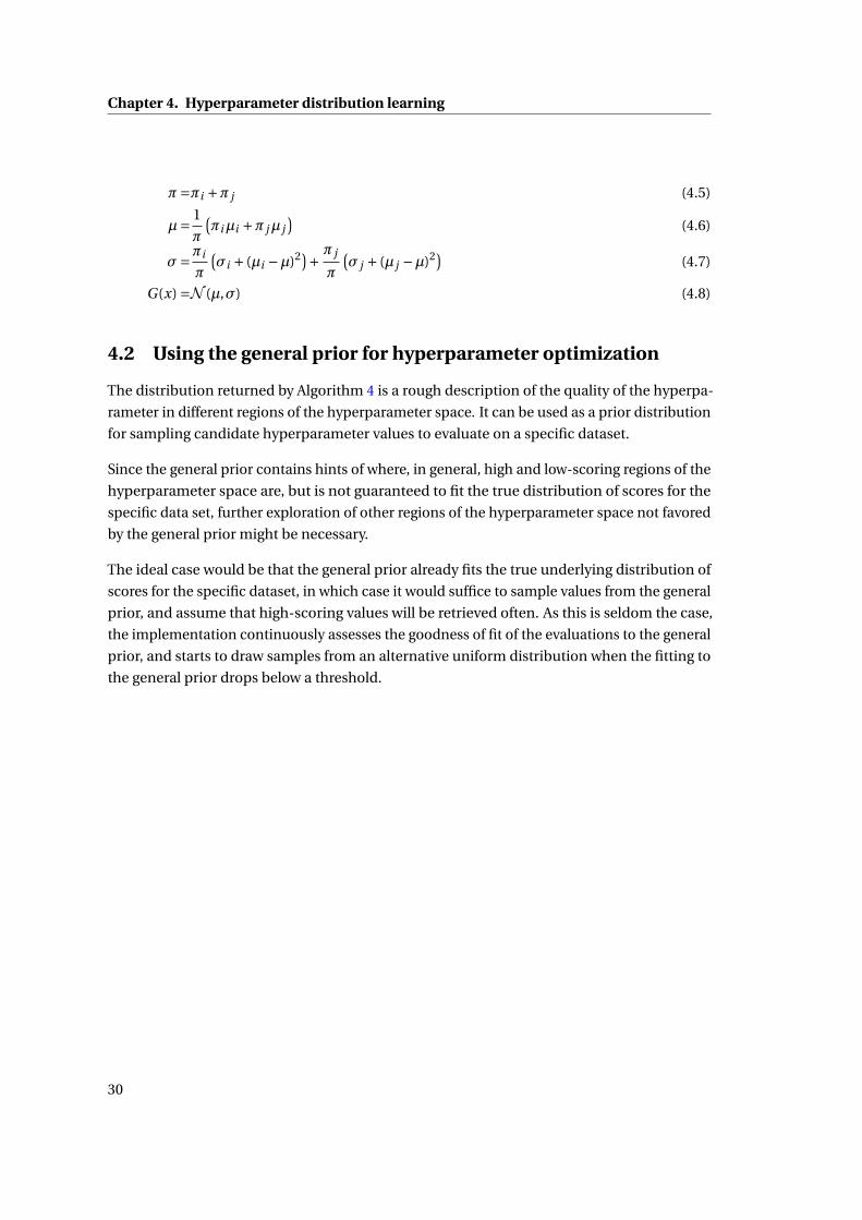
π=πi +π j (4.5)

µ= 1

π

(πiµi +π jµ j

)(4.6)

σ=πi

π

(σi + (µi −µ)2)+ π j

π

(σ j + (µ j −µ)2) (4.7)

G(x) =N (µ,σ) (4.8)

4.2 Using the general prior for hyperparameter optimization

The distribution returned by Algorithm 4 is a rough description of the quality of the hyperpa-

rameter in different regions of the hyperparameter space. It can be used as a prior distribution

for sampling candidate hyperparameter values to evaluate on a specific dataset.

Since the general prior contains hints of where, in general, high and low-scoring regions of the

hyperparameter space are, but is not guaranteed to fit the true distribution of scores for the

specific data set, further exploration of other regions of the hyperparameter space not favored

by the general prior might be necessary.

The ideal case would be that the general prior already fits the true underlying distribution of

scores for the specific dataset, in which case it would suffice to sample values from the general

prior, and assume that high-scoring values will be retrieved often. As this is seldom the case,

the implementation continuously assesses the goodness of fit of the evaluations to the general

prior, and starts to draw samples from an alternative uniform distribution when the fitting to

the general prior drops below a threshold.

30

CHAPTER 5Evaluation of results

The hyperparameter optimization and model selection process was run on a number of

datasets that include 29 standard datasets commonly used in the machine learning community,

and 8 datasets taken from biological experiments. The performance of the SML algorithms

under default settings was also computed for each dataset.

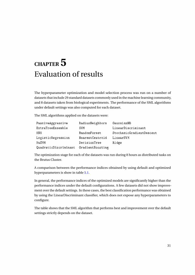
The SML algorithms applied on the datasets were:

PassiveAggressive RadiusNeighbors GaussianNB

ExtraTreeEnsemble SVM LinearDiscriminant

KNN RandomForest StochasicGradientDescent

LogisticRegression NearestCentroid LinearSVM

NuSVM DecisionTree Ridge

QuadraticDiscriminant GradientBoosting

The optimization stage for each of the datasets was run during 8 hours as distributed tasks on

the Brutus Cluster.

A comparison between the performance indices obtained by using default and optimized

hyperparameters is show in table 5.1.

In general, the performance indices of the optimized models are significantly higher than the

performance indices under the default configurations. A few datasets did not show improve-

ment over the default settings. In these cases, the best classification performance was obtained

by using the LinearDiscriminant classifier, which does not expose any hyperparameters to

configure.

The table shows that the SML algorithm that performs best and improvement over the default

settings strictly depends on the dataset.

31

Chapter 5. Evaluation of results

default OptimizedStandard ML datasets Worst Best Score Boost Familybalance-scale 0.0961 0.7452 0.8385 12.52% LinearSVMblood-transfusion 0.0553 0.2760 0.3307 19.80% NearestCentroidcmc -0.0607 0.1995 0.2458 23.23% KNNdermatology 0.3414 0.9292 0.9378 0.93% LinearSVMdiabetes -0.0582 0.4449 0.4454 0.11% Ridgehaberman -0.0599 0.1523 0.2746 80.37% LinearSVMheart-statlog -0.0300 0.6894 0.7036 2.05% Ridgeionosphere 0.5490 0.7839 0.8373 6.82% GradientBoostingiris 0.4250 0.9696 0.9841 1.50% KNNkdd_synthetic_control 0.0210 0.9987 1.0000 0.13% KNNletter 0.0920 0.8851 0.8851 0.00% KNNliver-disorders -0.1600 0.3198 0.3333 4.25% Ridgemfeat-factors -0.0002 0.9700 0.9700 0.00% LinearDiscriminantmfeat-fourier 0.0700 0.8143 0.8154 0.14% KNNmfeat-karhunen 0.4696 0.9431 0.9544 1.20% KNNmfeat-morphological -0.0230 0.6719 0.6719 0.00% LinearDiscriminantmfeat-pixel 0.6710 0.9522 0.9570 0.51% KNNmfeat-zernike -0.0000 0.7994 0.7994 0.00% LinearDiscriminantoptdigits 0.1663 0.9743 0.9803 0.61% QuadraticDiscriminantpage-blocks -1.8119 0.7864 0.7992 1.64% GradientBoostingpendigits 0.0063 0.9825 0.9877 0.53% KNNsegment-test 0.0180 0.9073 0.9152 0.87% GradientBoostingsonar -0.0775 0.5563 0.5890 5.88% LinearSVMspambase 0.0444 0.7786 0.8613 10.63% GradientBoostingtae -0.0165 0.3070 0.3385 10.28% LinearSVMvehicle -0.0484 0.6952 0.6978 0.37% QuadraticDiscriminantvowel 0.1243 0.6708 0.8250 22.98% KNNwaveform-5000 0.4915 0.7971 0.8025 0.68% Ridgewine -0.1486 0.9544 0.9544 0.01% RidgeBiological datasetsHK2_Standardized 0.5895 0.8060 0.8060 0.00% LinearSVMHuotari500_Standardized 0.2347 0.5238 0.5867 12.01% LinearSVMMeier500_Standardized 0.0499 0.8692 0.8748 0.66% GradientBoostingso -0.0444 0.8745 0.8987 2.77% LinearSVMWildMain500_Standardized 0.3048 0.8020 0.8269 3.11% LinearSVMyeast 0.0006 0.3758 0.4093 8.90% KNNcolonTumor 0.2198 0.7760 0.8540 10.05% Ridge

Table 5.1: Comparison of optimized and default performance indices for all datasets.

5.1 Results on standard Machine Learning datasets

Standard datasets are commonly used for testing and evaluating machine learning approaches.

Some of the datasets used here are inherently difficult to classify, and hence most SML algo-

32

5.2. Results on biological data

rithms consistently obtain a very low performance index; other datasets are simple to classify

and hence good performance indices are expected. Since good predictions may also be ob-

tained by using the default values, little relative improvement (of the best model over the

default values) is also expected.

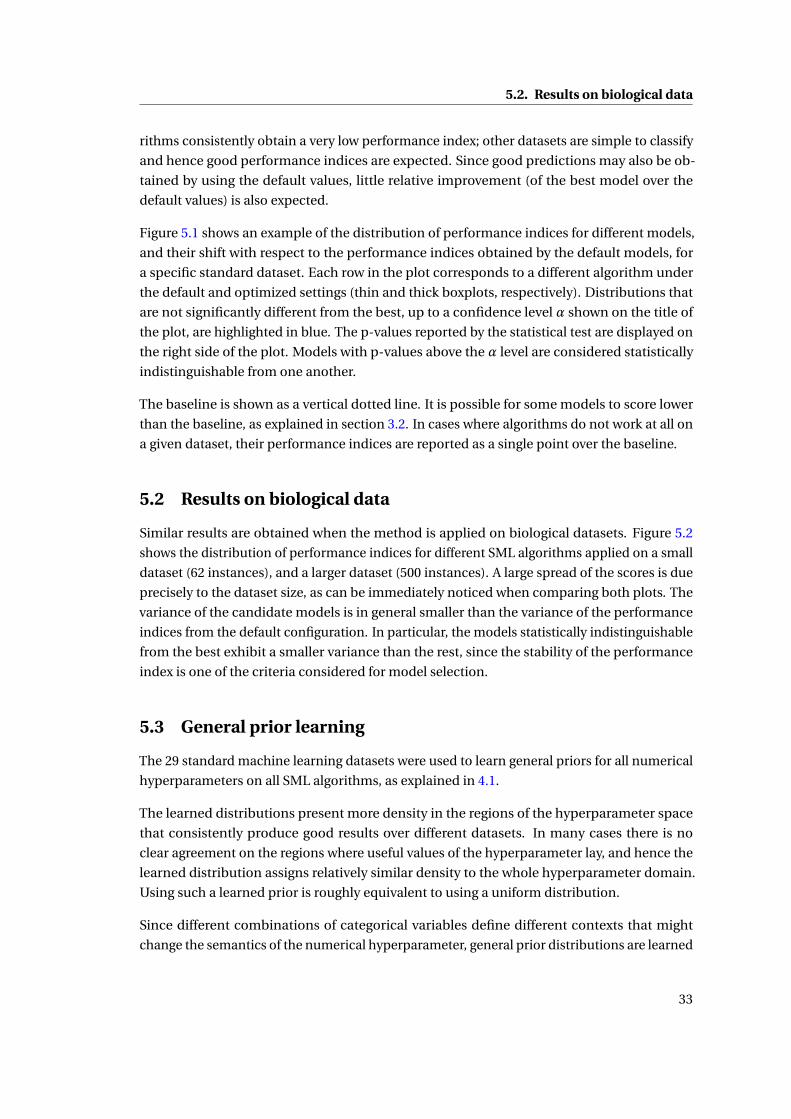
Figure 5.1 shows an example of the distribution of performance indices for different models,

and their shift with respect to the performance indices obtained by the default models, for

a specific standard dataset. Each row in the plot corresponds to a different algorithm under

the default and optimized settings (thin and thick boxplots, respectively). Distributions that

are not significantly different from the best, up to a confidence level α shown on the title of

the plot, are highlighted in blue. The p-values reported by the statistical test are displayed on

the right side of the plot. Models with p-values above the α level are considered statistically

indistinguishable from one another.

The baseline is shown as a vertical dotted line. It is possible for some models to score lower

than the baseline, as explained in section 3.2. In cases where algorithms do not work at all on

a given dataset, their performance indices are reported as a single point over the baseline.

5.2 Results on biological data

Similar results are obtained when the method is applied on biological datasets. Figure 5.2

shows the distribution of performance indices for different SML algorithms applied on a small

dataset (62 instances), and a larger dataset (500 instances). A large spread of the scores is due

precisely to the dataset size, as can be immediately noticed when comparing both plots. The

variance of the candidate models is in general smaller than the variance of the performance

indices from the default configuration. In particular, the models statistically indistinguishable

from the best exhibit a smaller variance than the rest, since the stability of the performance

index is one of the criteria considered for model selection.

5.3 General prior learning

The 29 standard machine learning datasets were used to learn general priors for all numerical

hyperparameters on all SML algorithms, as explained in 4.1.

The learned distributions present more density in the regions of the hyperparameter space

that consistently produce good results over different datasets. In many cases there is no

clear agreement on the regions where useful values of the hyperparameter lay, and hence the

learned distribution assigns relatively similar density to the whole hyperparameter domain.

Using such a learned prior is roughly equivalent to using a uniform distribution.

Since different combinations of categorical variables define different contexts that might

change the semantics of the numerical hyperparameter, general prior distributions are learned

33

Chapter 5. Evaluation of results

0.0 0.2 0.4 0.6 0.8 1.0

Performance index

PassiveAggressive

RadiusNeighbors

GaussianNB

ExtraTreeEnsemble

SVM

LinearDiscriminant

KNN

RandomForest

SGD

LogisticRegression

NearestCentroid

LinearSVM

NuSVM

DecisionTree

Ridge

QuadraticDiscriminant

GradientBoosting

Dataset: sonar. α=0.85

mean default parameters significant difference non-significant difference

(>= 0.9)

(<= 0.001)

(<= 0.001)

0.0013

0.0069

(<= 0.001)

0.0396

0.0165

(>= 0.9)

(>= 0.9)

0.2117

0.003

0.0937

0.705

(<= 0.001)

0.4333

p-v

alu

e (

wit

h r

esp

ect

to t

he b

est

)

Figure 5.1: Optimized vs default values for a standard machine learning dataset

independently for each categorical context.

As an example, we present the learned distributions of the hyperparameter γ for two different

kernels used by a support vector machine classifier. Plots of the learned distributions are

shown in Figure 5.3

As evidenced in the plots, some categorical hyperparameters may or may not influence the

distribution of the numerical hyperparameters. The value of the shrinking hyperparameter in

this case does not significantly alter the distribution of γ.

The distributions learned by analyzing the values of γ for a polynomial kernel, shown in the

34

5.3. General prior learning

0.0 0.2 0.4 0.6 0.8 1.0

Performance index

PassiveAggressive

RadiusNeighbors

GaussianNB

ExtraTreeEnsemble

SVM

LinearDiscriminant

KNN

RandomForest

SGD

LogisticRegression

NearestCentroid

LinearSVM

NuSVM

DecisionTree

Ridge

QuadraticDiscriminant

GradientBoosting

Dataset: colonTumor. α=0.85

mean default parameters significant difference non-significant difference

0.4333

(<= 0.001)

(<= 0.001)

0.0396

0.0937

(<= 0.001)

0.2117

0.0165

(>= 0.9)

0.705

(>= 0.9)

(>= 0.9)

0.0069

0.0013

(<= 0.001)

0.003

p-v

alu

e (

wit

h r

esp

ect

to t

he b

est

)

0.0 0.2 0.4 0.6 0.8 1.0

Performance index

PassiveAggressive

RadiusNeighbors

GaussianNB

ExtraTreeEnsemble

SVM

LinearDiscriminant

KNN

RandomForest

SGD

LogisticRegression

NearestCentroid

LinearSVM

NuSVM

DecisionTree

Ridge

QuadraticDiscriminant

GradientBoosting

Dataset: WildMain500_Standardized. α=0.85

mean default parameters significant difference non-significant difference

0.705

(<= 0.001)

(<= 0.001)

0.0069

0.003

(<= 0.001)

0.4333

0.0396

(>= 0.9)

0.0937

(>= 0.9)

0.0013

0.0165

(>= 0.9)

(<= 0.001)

0.2117

p-v

alu

e (

wit

h r

esp

ect

to t

he b

est

)

Figure 5.2: Optimized vs default values for biological datasets of different sizes. The colonTumor dataset contains62 instances, whereas the WildMain500_Standarized dataset contains 500 instances.

top row of Figure 5.3, look similar, regardless of the value of other categorical hyperparameters.

Both distributions assign a rather uniform density over the entire (0,1) domain. No important

improvement in the optimization process should be expected when such distribution is used

as a general prior.

The bottom row of Figure 5.3 shows the learned general prior for the same numerical hyper-

parameter γ when used in combination with a sigmoid kernel. In this case, the evaluation

of the hyperparameter on the large group of datasets seems to achieve better performance

when small values (close to zero) are used, although the assignment of values away from zero

is also allowed. This skewness of the learned distribution, when using a sigmoid kernel, may

be exploited when looking for optimal values of γ on other datasets, as a suggestion of where

to look first.

35

Chapter 5. Evaluation of results

class_weight:auto, kernel:poly, shrinking:True

0.5 0.0 0.5 1.0 1.5γ

0.0

0.2

0.4

0.6

0.8

1.0

1.2

1.4

1.6class_weight:auto, kernel:poly, shrinking:False

0.5 0.0 0.5 1.0 1.5γ

0.0

0.2

0.4

0.6

0.8

1.0

1.2

1.4

1.6

class_weight:auto, kernel:sigmoid, shrinking:True

0.5 0.0 0.5 1.0 1.5γ

0.0

0.2

0.4

0.6

0.8

1.0

1.2

1.4

1.6class_weight:auto, kernel:sigmoid, shrinking:False

0.5 0.0 0.5 1.0 1.5γ

0.0

0.2

0.4

0.6

0.8

1.0

1.2

1.4

1.6

Figure 5.3: Distributions of the γ hyperparameter learned from the performance indices over a large group ofdatasets. The title over each plot indicates the signature of the categorical context (i.e., the values of the categoricalhyperparameters).

36

CHAPTER 6Conclusion

This work shows that an automatic approach to hyperparameter optimization and model

selection is very valuable, especially when little knowledge of the internal function and config-

uration options of the SML algorithms is available. The optimized configurations retrieved

by our approach significantly boosted the predictive power of most SML algorithms over

their defaults. Moreover, the models optimized and selected by our method consider other

preferable criteria such as the runtime, stability of the scores, and predictive generalization to

unseen instances.

Furthermore, the automated procedure described here is very convenient for non-experts,

as using this method requires training in machine learning that does not go beyond the

general concepts. Our method is already a valuable tool that brings SML algorithms closer

to the untrained user, and narrows the gap between the purely-technical machine learning

community and the vast range of other disciplines that might benefit from SML techniques.

An important consideration regarding the optimization process is that, since the optimization

happens simultaneously on a large group of numerical hyperparameters, finding good combi-

nations of hyperparameters may be a slow process. The choice of an optimization method

that makes use of the optimization history and other hints to guide the sampling of candidate

configurations is critical when time is a concern.

6.1 Future work

Many possibilities to extend this work are considered, and planned. The most important ones

are described next.

Optimization methods

Implementing more sophisticated optimization methods is the obvious next step. Opti-

mization methods such as simulated annealing or genetic algorithms may speed up the

hyperparameter optimization. Other methods such as may be implemented in the future.

37

Chapter 6. Conclusion

Data preprocessing

In most real-world applications, the raw data obtained from experiments is not immediately

suitable for training SML algorithms. Data with high dimensionality (many features) usually

requires lots of computational resources, and the large number of dimensions can make a

very informative signal (i.e., a dimension or group of dimensions that correlate well with the

labeling) difficult to detect among all the rest of non-informative dimensions.

Feature selection and dimensionality reduction techniques should be included as a prepro-

cessing step. The decision on which dimensionality reduction to use can also be regarded as a

categorical hyperparameter of the model selection process, and included as part of the final

suggestion of a best model.

Dataset classification

Having a framework that automatically finds the best model for specific data might be used

on a larger scale to infer patterns between dataset-wide features and the SML algorithms that

best predict on them. Approaches such as the one presented in [?], where a distance metric

between two datasets is suggested, can be further investigated. Finding dataset-wide features

that follow patterns according to the SML algorithms best suited for them might also be used

as a first clue of what SML algorithms could work well on a specific dataset.

Custom penalization of misclassifications

Some misclassifications may be more tolerable than others, for data of a certain nature. Penal-

ization of misclassifications can be modified by using a custom confusion matrix that weights

misclassifications accordingly. All the metrics that evaluate the quality of the prediction in

terms of the true or false positives and negatives should use those weights in their internal

computations.

38

APPENDIX ASupervised machine learning algorithms

The following SML algorithms are used in this work:

Name Description

KNN k-nearest neighbors classifier.

RadiusNeighbors Votes among neighbors within a certain radius.

NearestCentroid Assigns the class of the centroid of the nearest cluster.

StochasicGradientDescent Stochastic Gradient Descent classifier.

LogisticRegression Logistic function applied on a linear combination of fea-

tures.

SVM Support Vector Machine (libSVM implementation).

LinearSVM Linear SVM (libLinear implementation).

NuSVM Nu-Support Vector Machine.

DecisionTree Decision tree classification.

RandomForest Average of multiple decision trees on subsets of the data.

ExtraTreeEnsemble Random forest with randomized decision trees.

Ridge Least squares regression with L2 loss.

LinearDiscriminant Linear discriminant analysis.

QuadraticDiscriminant Quadratic discriminant analysis.

GradientBoosting An ensemble of regression tree classifiers.

PassiveAggressive Passive Aggressive classifier.

GaussianNB Gaussian Naïve Bayes classifier

39

APPENDIX BDatasets

Standard datasets Instances Features Classes

balance-scale 625 4 3

blood-transfusion 748 4 2

cmc 1473 9 3

dermatology 366 34 6

diabetes 768 8 2

haberman 306 4 2

heart-statlog 270 13 2

ionosphere 351 34 2

iris 150 4 3

kdd_synthetic_control 600 60 6

letter 20000 16 26

liver-disorders 345 7 2

mfeat-factors 2000 649 10

mfeat-fourier 2000 649 10

mfeat-karhunen 2000 649 10

mfeat-morphological 2000 649 10

mfeat-pixel 2000 649 10

mfeat-zernike 2000 649 10

optdigits 3823 64 10

page-blocks 5473 10 5

pendigits 7494 16 10

segment-test 2100 19 7

sonar 208 60 2

spambase 4601 57 2

tae 151 5 3

vehicle 946 18 4

vowel 990 14 11

waveform-5000 5000 21 3

wine 178 13 3

41

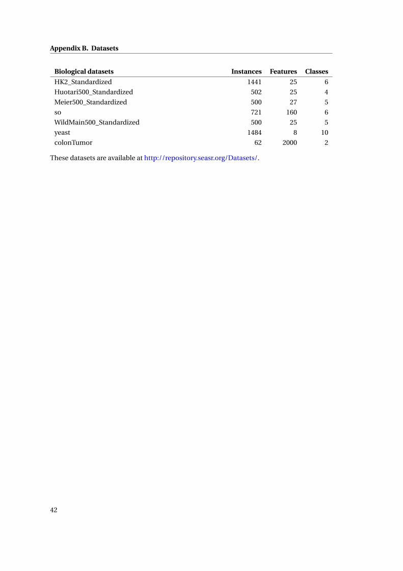
Appendix B. Datasets

Biological datasets Instances Features Classes

HK2_Standardized 1441 25 6

Huotari500_Standardized 502 25 4

Meier500_Standardized 500 27 5

so 721 160 6

WildMain500_Standardized 500 25 5

yeast 1484 8 10

colonTumor 62 2000 2

These datasets are available at http://repository.seasr.org/Datasets/.

42