permanent freight data collection infrastructure and

1

Permanent Freight Data Collection

Infrastructure and Archive System

TECHNICAL MEMORANDUM #1

Portland State University

Oregon State University

January 2013

2

TABLE OF CONTENTS

1 INTRODUCTION ....................................................................................................................... 4

2 LENGTH BASED CLASSIFICATION ............................................................................................ 4

2.1 State of the Practice ......................................................................................................... 5

2.1.1 Length-Based Pooled Fund Study ............................................................................. 5

2.1.2 U.S. Department of Transportation, Federal Highway Administration (FHWA) ...... 6

2.1.3 Washington Department of Transportation (WSDOT) ............................................. 7

2.1.4 Wisconsin Department of Transportation (WisDOT) ............................................... 8

2.1.5 Hawaii Department of Transportation (HDOT) ........................................................ 8

2.1.6 Minnesota Department of Transportation (MnDOT) ............................................... 9

2.1.7 Florida Department of Transportation (FDOT) ......................................................... 9

2.1.8 Ohio Department of Transportation ....................................................................... 10

2.1.9 New York Study ....................................................................................................... 10

2.2 Summary of Length Bins ................................................................................................ 10

2.3 Peer Reviewed Literature ............................................................................................... 11

2.3.1 Length-Based Classification from Single Loops ...................................................... 11

2.3.2 Length-Based Classification from Dual Loops ......................................................... 11

2.3.3 Length-Based Classification from Video ................................................................. 12

3 TECHNOLOGY REVIEW .......................................................................................................... 13

3.1 INDUCTIVE LOOP DETECTORS ........................................................................................ 14

3.1.1 Preformed Loops ..................................................................................................... 15

3.1.2 Saw-Cut Loops ......................................................................................................... 15

3.1.3 Loop Extension Cable .............................................................................................. 15

3.1.4 Number of Outputs ................................................................................................. 15

3.1.5 Signal Type .............................................................................................................. 16

3.1.6 Diagnostics .............................................................................................................. 16

3.2 LOOP INSTALLATION AND SENSITIVITY .......................................................................... 16

3.2.1 Sensitivity ................................................................................................................ 16

3.2.2 Troubleshooting ...................................................................................................... 20

3

3.3 INDUCTIVE LOOP DETECTOR MANUFACTURERS ........................................................... 20

3.3.1 RENO A&E ............................................................................................................... 21

3.3.2 Summary ................................................................................................................. 25

4 REFERENCES .......................................................................................................................... 25

5 APPENDIX A ........................................................................................................................... 26

6 APPENDIX B ........................................................................................................................... 32

7 APPENDIX C ODOT WIM Classification ................................................................................ 34

4

1 INTRODUCTION

Truck classification data can be the useful inputs for traffic monitoring programs, freight

mobility studies, infrastructure design projects and long-range planning models. Trucking

movements have very unique characteristics due to their heavy weight and large turning radii.

These characteristics make truck classification an important element for traffic operation,

safety and planning. Collecting truck classification data can be a useful tool to relate truck

counts, freight mobility studies, and structure design projects. There are several different ways

to detect different types of trucks, such as travel surveys, video image detection, and

single/dual loop detectors.

The main focus of this part of the project was to review length-based classification schemes,

technologies, and to gain a better understanding of how inductive loop sensors and detectors

work and to acquire the required parts to set up a test inductive loop detector system. This

report present the review in two parts: 1) length-based classification and 2)technology

overview.

2 LENGTH BASED CLASSIFICATION

The FHWA’s Traffic Monitoring Guide: Section 4 Vehicle Classification Monitoring (FHWA 2001)

summarizes a number of issues related to vehicle classification by both number of axle and

length of vehicles. In many counts, classification is done by visually classifying trucks on the

basis of a vehicle's body style. For permanent or long-term counts, vehicle classification is done

by either an axle-based or length-based method.

There are several common detection methods for classifying vehicles such as the one above:

Axle Sensor Based Counters - Measuring the number of axles associated with each

passing vehicle and the spacing between axles, by computing the speed of the vehicle

and the time between axle pulses on each sensor.

Vehicle Length Based Counters - Using two inductive loops estimate the total length of

vehicles crossing the loops. Vehicle length is computed by dividing the total time a

vehicle is over the loop by the speed of that vehicle. Radar units can also measure

vehicle length.

Machine Vision Based Equipment - Machine vision systems are based on video image

processing. Camera systems allow the detector to be placed above or beside the

roadway; this provides a significant advantage for locations where access to the

roadway is extremely limited and expensive, such as high volume urban freeways.

The schematic in Figure 1 below illustrates a typical 5-axle semi-truck trailer combination. Note

that both the axle numbers and spacing provide details about the type of vehicle.

5

Figure 2-1 Typical 5-axle semi-truck configuration

2.1 State of the Practice

2.1.1 Length-Based Pooled Fund Study

The FHWA recently completed a length-based pooled fund study. The comprehensive study

suggested the following:

Figure 2-2 From Pooled Fund Study

6

2.1.2 U.S. Department of Transportation, Federal Highway Administration (FHWA)

The federal classification scheme includes 13 vehicles (see Appendix A). The FHWA classification

scheme is separated into different categories. These categories are dependent on whether the

vehicle carries passengers or commodities. In addition, the number of axles and number of

units create the division between vehicles which carry passengers and vehicles which carry

commodities.

In order to correctly classify vehicles into the aforementioned categories, algorithms are

needed to interpret axle spacing information. These algorithms must be implemented on

automatic vehicle classifiers (ATC). These algorithms are commonly used based on “Scheme F”

which was developed by the USDOT in the mid-80s. Table 1 represents “Scheme F”.

Table 1: “Scheme F” Number of Axles per Vehicle

The FHWA does not recommend “Scheme F” or any other classification algorithm. They have

concluded that axle spacing characteristics for specific vehicle types vary from state to state

thus there is no general spacing standards for all cases. In order to achieve accurate results, it is

up to state DOT’s and agencies to develop, test and improve an algorithm.

The FHWA proposed a new classification method, which is based on the aggregation of the

“Scheme F” classification. This classification scheme was tested using the combined data from

all states.

7

Table 2 represents the length based classification boundaries and the errors associated with it,

respectively.

8

Table 2: Length Based Classification Boundaries

In order to get better results, fine-tuning the length spacing boundaries to account for

characteristics of their trucking fleets would improve these errors. However, fine-tuning will not

always lead to a perfect length classification scheme since total vehicle length is not a

consistent indicator of a vehicle class, thus size and type of misclassification errors should be

considered in order to minimize error. The TMG highlights that all of the detection technologies

have “difficulty classifying vehicles in conditions where vehicles do not operate at constant

speed, where vehicles follow very closely, or where stop and go traffic occurs”.

Using only length, vehicles will almost certainly be classified incorrectly. For example, a 34 feet

small tractor-trailer combination would be classified by length as bin 2 (SU). However, knowing

it has three axles and the spacing of those axles it would more likely be classified correctly as

combination unit (CU) vehicle. Table 3 presents information from the TMG which reports

classification errors comparing a length-only classification to a number of axles and spacing

classification. Correct classifications are highlighted in bold while incorrect classifications are

italicized. The table highlights that length-based classification will have challenges

distinguishing long passenger cars and single unit trucks and combination and multi-trailer

trucks because of the diversity of configurations.

Table 3: Misclassification Errors Caused By Using Only Total Vehicle Length as the Classification

Classification Based on Total Vehicle Length

Classification PV SU CU MU

Based on SU 17.7% 81.9% 0.4% 0%

Configuration and CU 0% 1.8% 84.2% 14.0%

Number of Axles MU 0% 0.1% 20.8% 79.1%

Source: TMG

2.1.3 Washington Department of Transportation (WSDOT)

Washington State DOT uses dual loops in their freeway detection system in order to classify

vehicles according to their length. They use four length-based vehicle categories. The four

length-based category is described in

9

Table 4.

10

Table 4 Four Length-Based Vehicle Categories Used by the WSDOT

Wang and Nihan et al. did a study and determined that during peak hours and off-peak hours

dual-loop detectors mistakenly assign bin three vehicles to bin four vehicles, however the

reverse (bin four to bin three) does not occur. In addition, they found out that dual-loop

detectors have problems in differentiating bin two vehicles from bin three vehicles. They also

concluded that in off-peak hours, 30 to 41 percent of misclassification errors are observed for

trucks.

2.1.4 Wisconsin Department of Transportation (WisDOT)

WisDOT also used dual loop detectors in order to estimate the length of vehicles. They

considered a five-length bin classification scheme, however they used a three length bin

classification and examined average absolute estimation error. They concluded that errors were

too small and when an estimate fell outside of the correct bin a “buffer zone” was created

between three bins. Errors were then shown if they were correct or incorrect, in addition to the

percent of the error. Table 5 shows the three-bin classification.

Table 5: WisDOT Classification Scheme

Bin Range

1 0-22ft

2 22-40ft

3 over 40ft

2.1.5 Hawaii Department of Transportation (HDOT)

HDOT classified vehicle length using Autoscope sensor and SmartSensor HD with The Infra-Red

Traffic Loggerr (TIRTL). They suggested a 5-class scheme, which is shown in Table 6.

Table 6: HDOT Vehicle Classification

Class Range Type

A 0-13 ft Motor cycle and moped

B 13-22 ft Passenger vehicle, Truck tractor, Pickup truck, mid-size SUV

C 22-42 ft Conventional bus and single-unit truck

D 42-62 ft articulated bus and single trailer combination truck

E over 62 ft multiple-trailers combination truck

11

Using Autoscope sensor and SmartSensor HD, HDOT concluded that the proposed classification

scheme tends to minimize the overlapping of vehicle type, however it does not eliminate this

deficiency. In addition, they concluded that most of the errors occurred while classifying class C

and D.

Using the TIRTL sensor, they concluded that the system provides adequate accuracy of FHWA

axle-based classification and it’s best if used for industrial freeways. Having said that, TIRTL

requires flat pavement without pronounced crowns in order to be deployed and have the best

results. In addition, they concluded that the majority of misclassification occurs in the

differentiation between class 2 (passenger cars) and class 3 (pickups).

2.1.6 Minnesota Department of Transportation (MnDOT)

In 2005, MnDOT recommended the use of four bins for their length-based classification. Table 7

describes MnDOT’s classification.

Table 7: MnDOT Vehicle Classification

Vehicle Type Vehicle Length Vehicle Class

Motorcycle 0 to 7 ft 1

Passenger Vehicles (PV) 7 to 22 ft 2 & 3

Single Unit Truck (SU) 22 to 37 ft 4 to 7

Combination Trucks (MU over 37 ft 8 to 13

In 2010, Erik Minge conducted research to evaluate non-intrusive technologies for traffic

detection. He compared technologies such as Wavetronix Smart Sensor HD, GTT Canoga

Microloops, Peek AxleLight and TIRTL. In this research he concluded that a length-based sensor

provides better data regarding its accuracy in comparison with the axle-based sensors. In

addition, he suggested that different agencies and state DOT’s should perform independent

analysis of their classification schemes to determine the best result for their existing sensors.

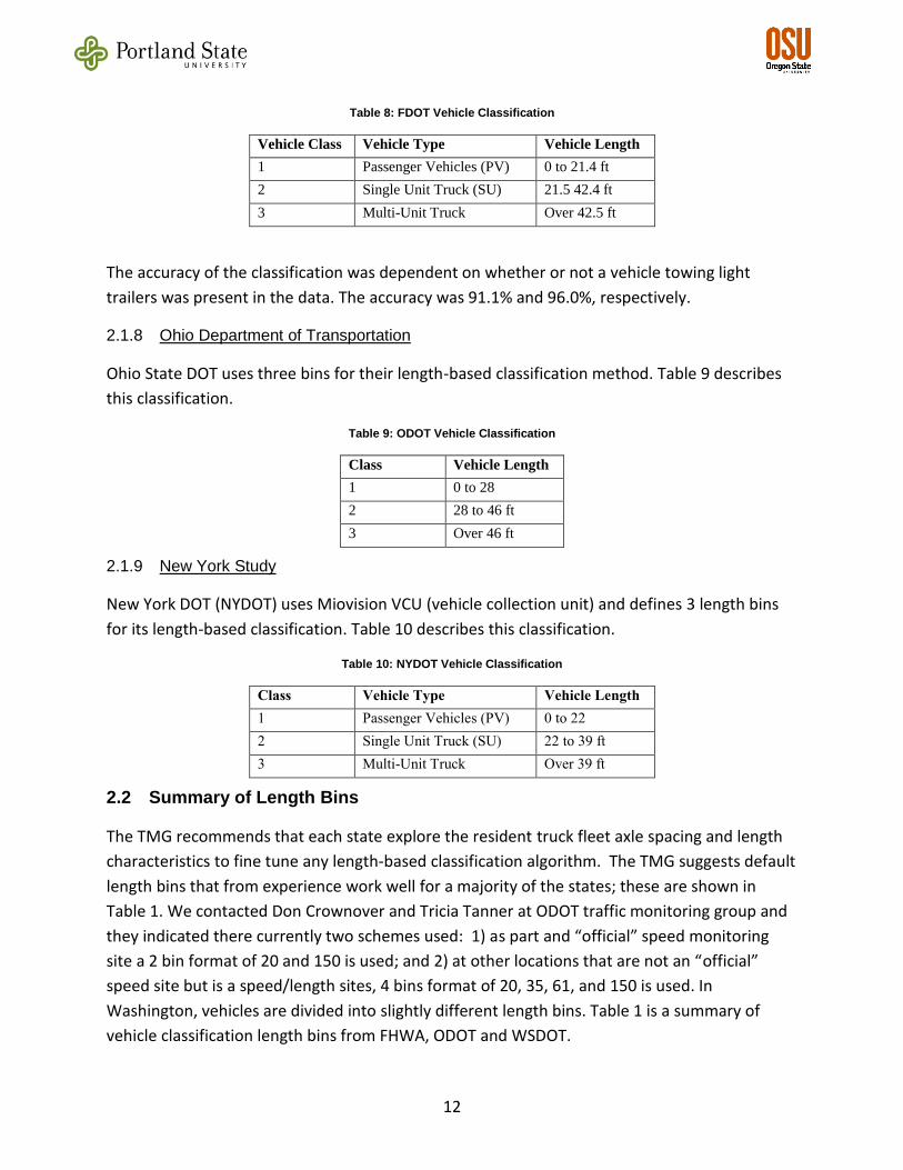
2.1.7 Florida Department of Transportation (FDOT)

FDOT collected data using video capture. The length of vehicles was extracted using specialized

analysis software and classified into “Scheme F” of FHWA. They concluded that there were

overlaps among vehicle classes 4, 5, 6 and 7 between the ranges of 25 to 40 feet. In addition,

they concluded that there are overlaps of lengths of vehicle classes 8, 9 and 10 from 43 to 80

feet. FDOT suggested using a pattern recognition technique in order to get the optimum length

threshold to have reasonable correspondence to FHWA “Scheme F”. They used the support

vector machines (SVM) model and classified vehicles into three bins. Table 8 describes the

classification.

12

Table 8: FDOT Vehicle Classification

Vehicle Class Vehicle Type Vehicle Length

1 Passenger Vehicles (PV) 0 to 21.4 ft

2 Single Unit Truck (SU) 21.5 42.4 ft

3 Multi-Unit Truck Over 42.5 ft

The accuracy of the classification was dependent on whether or not a vehicle towing light

trailers was present in the data. The accuracy was 91.1% and 96.0%, respectively.

2.1.8 Ohio Department of Transportation

Ohio State DOT uses three bins for their length-based classification method. Table 9 describes

this classification.

Table 9: ODOT Vehicle Classification

Class Vehicle Length

1 0 to 28

2 28 to 46 ft

3 Over 46 ft

2.1.9 New York Study

New York DOT (NYDOT) uses Miovision VCU (vehicle collection unit) and defines 3 length bins

for its length-based classification. Table 10 describes this classification.

Table 10: NYDOT Vehicle Classification

Class Vehicle Type Vehicle Length

1 Passenger Vehicles (PV) 0 to 22

2 Single Unit Truck (SU) 22 to 39 ft

3 Multi-Unit Truck Over 39 ft

2.2 Summary of Length Bins

The TMG recommends that each state explore the resident truck fleet axle spacing and length

characteristics to fine tune any length-based classification algorithm. The TMG suggests default

length bins that from experience work well for a majority of the states; these are shown in

Table 1. We contacted Don Crownover and Tricia Tanner at ODOT traffic monitoring group and

they indicated there currently two schemes used: 1) as part and “official” speed monitoring

site a 2 bin format of 20 and 150 is used; and 2) at other locations that are not an “official”

speed site but is a speed/length sites, 4 bins format of 20, 35, 61, and 150 is used. In

Washington, vehicles are divided into slightly different length bins. Table 1 is a summary of

vehicle classification length bins from FHWA, ODOT and WSDOT.

13

Table 11: Length Based Classification Boundaries

Vehicles Classification Range of Length (in ft)

Pooled Fund (Urban)

Pooled Fund (Rural)

FHWA TMG

ODOT WSDOT

Passenger vehicles (PV) > 20 > 21.5 > 13 > 20 > 26

Single unit trucks (SU) 20 to 43 21.5 to 49 13 to 35 20 to 35 26 to 39

Combination trucks (CU)

36 to 61 36 to 60 40 to 65

Multi-trailer trucks (MU)

> 43 > 49 62 to 120 61 to 150

> 65

2.3 Peer Reviewed Literature

2.3.1 Length-Based Classification from Single Loops

Because single-loops are a more common deployment for freeway management, a number of

papers have explored using single-loop detectors to do the work of dual loops including length-

based classification. Wang and Nihan illustrated that for a typical freeway location on I-5 in

Washington, the distribution of vehicle lengths clearly indicated a hi-normal distribution with

two distinct peaks. Shorter vehicles had a mean length of 5.5 m (18.0 ft) and a standard

deviation of 0.9 m (3.0 ft), while long vehicles had a mean length of 22.5 m (73.8 ft) and a

standard deviation of 3.6 m (11.8 ft) (Wang and Nihan 2004)(Wang and Nihan 2003).

Coifman presented the new speed estimation techniques from output from single loop

detector, compare with dual loop detector measurement. Following the Ohio Department of

Transportation length based on classification scheme for dual detectors, the lengths are used to

classify vehicles into three bins with divisions at effective vehicle lengths of 28 ft and 46ft.

In 2008, Coifman and Kim from Ohio State University developed a new methodology in order to

use single-loop detectors for length-based classification. They also evaluated this methodology

to the existing measurements from video and dual-loop detectors. They concluded that

classification results from single-loop detectors were very close to those from dual-loop

detectors, however they did not suggest the use of single-loop detectors until more research

was done.

2.3.2 Length-Based Classification from Dual Loops

A very relevant study was conducted by Zhang et al (2005) in Seattle, Washington. The

researchers evaluated the accuracy of dual-loop measurements of volume and vehicle

14

classifications and developed methods for improving the quality of real-time dual-loop

measurements. This was accomplished by comparing the loop detector measurements and

ground-truth data collected (video images) at two different locations. Zhang et al found that

dual-loop detectors tend to underestimate total vehicle volumes (Bin 3 vehicles often were

considered as being in Bin 4) though the reverse never occurs and that dual-loop detectors

have difficulties identifying Bin 2 vehicles. Publicly available software (DEDAC) for dual-loop

detectors was produced as part of this research effort.

Ai and Wei did a study to evaluate the dual-loop length-based vehicle classification models

against the ground-truth vehicle trajectory data extracted from video under different traffic

conditions, free flow, synchronized flow and stop-and-go flow. It is important to note that in

synchronized flow, traffic flow is lower than that of the free flow. In stop-and-go flow, vehicles

will stop within the detection area frequently for at least one time, which was defined by

Kerner et al.

In order to develop this new model, ground-truth data was collected from video vehicle

trajectory using VEVID (video-capture-based technique) to extract high-resolution vehicle

trajectory. They also used a probe vehicle, which was equipped with a Global Positioning

System (GPS) traveler data logger to collect traffic pattern data in order to validate parameters

that were involved in the new vehicle classification models. They proposed two new models,

VC-Sync model (Vehicle Classification Model under Synchronized traffic) and VC-Stog model

(Vehicle Classification Model under Stop-and-Go Traffic).

They concluded that the VC-Sync model significantly increased the accuracy of vehicle

classification against synchronized and stop-and-go traffic conditions. Using the VC-Sync model

reduced the error to 8.5% as compared to the existing model, which had an error of 35.2%. In

addition, using the VC-Stog model reduced the error to 27.7% as compared to the existing

model error of 210%.

2.3.3 Length-Based Classification from Video

As part of an earlier effort to do short/long vehicle classification using the existing data stream

in Portland, OR, Bertini et al (2006) compared video-based length classification (Autoscope) and

an implementation of Wang-Nihan algorithm. In this study they assumed that the dual-loop

outputs were from single loops (the algorithm uses volumes, occupancy, speed). Four locations

were used:

I-5 SB at Marine Drive in North Portland, OR

I-84 WB at Sandy Blvd/37th Ave in Southeast Portland, OR

I-5 NB at Lower Boones Ferry Road in Tualatin, OR

OR-217 at SW Hall Blvd. in Tigard, OR

15

An example of the length-distribution for one lane from the camera analysis is shown below

(which appears to be truncated at 50 feet for graphical purposes).

Figure 2: Autoscope Speed Detector Vehicle Length Histogram, Hour 14, Center Lane

Implementation of the Wang-Nihan algorithm using the PORTAL data was less than perfect (as

expected). In certain situations, the algorithm did a good job of predicting long vehicle volumes.

In others, the algorithm over or underestimates long vehicles. The analysis of the estimation

error patterns were inconclusive – there are inconsistencies during period of heavy traffic and

light traffic, both when the volume of trucks is low, and when trucks constitute a larger

percentage of the traffic stream.

Coifman and Lee also looked at LIDAR (light detection and ranging) technology in order to

develop a vehicle classification algorithm. LIDAR technology has been used in different

transportation applications in the past, such as highway safety and design. In addition, few

research has been done related to vehicle classification. In this study, they separated occluded

from non-occluded vehicles. Out of 27,000 vehicles, which were collected from ground truth

video, 11% were occluded. From the remaining non-occluded vehicles, 99.5% of them were

correctly classified.

3 TECHNOLOGY REVIEW

The primary purpose of this section of the report was to provide the background information

required to develop the sensors.

16

3.1 INDUCTIVE LOOP DETECTORS

As depicted in Figure 1, an inductive loop vehicle detector system consists of three

components: a loop (preformed or saw-cut), loop extension cable and a detector.

Figure 1. basic components of an inductive loop vehicle detector system

The preformed or saw-cut loop is buried in the traffic lane. The loop is a continuous run of wire

that enters and exits from the same point. The two ends of the loop wire are connected to the

loop extension cable, which in turn connects to the vehicle detector. The detector powers the

loop causing a magnetic field in the loop area. The loop resonates at a constant frequency that

the detector monitors. A base frequency is established when there is no vehicle over the loop.

When a large metal object, such as a vehicle, moves over the loop, the resonate frequency

increases. This increase in frequency is sensed and, depending on the design of the detector,

forces a normally open relay to close. The relay will remain closed until the vehicle leaves the

loop and the frequency returns to the base level.

In general, a compact car will cause a greater increase in frequency than a full size car or truck,

as depicted in Figure 2. This occurs because the metal surfaces on the under carriage of the

vehicle are closer to the loop.

Figure 2. Magnetic signatures of two different vehicle sizes

17

Detection is based on metal surface area, otherwise known as skin effect. The greater the

surface area of metal in the same plane as the loop, the greater the increase in frequency.

Figure 3 depicts another way to illustrate the point. In the left hand side of Figure 3, a one foot

square piece of sheet metal is easily detected by the loop since it is presented in the same

plane. However, if this same piece of sheet metal it is turned perpendicular to the loop (right

hand side of Figure 3), it becomes impossible to detect.

Figure 3. Detection capabilities of an inductive loop detector

3.1.1 Preformed Loops

A preformed loop is typically 3 to 5 turns of loop wire encased in PVC pipe for use in new

construction before the pavement is installed. The loop wire is 14 or 16 American Wire Gauge

(AWG) stranded machine tool wire with an insulation of cross-linked polyethylene (XLPE)

encased in a polyvinyl chloride (PVC) pipe to hold the loop’s shape and to protect the loop wire

from damage while the pavement is installed.

3.1.2 Saw-Cut Loops

A saw-cut loop is used when the pavement is already in place. The installation involves cutting

the loop shape in the pavement with a concrete saw, laying the loop wire in the slot, pressing in

a polyfoam backer rod to keep the wire compacted and finishing with saw-cut loop sealant or

street bondo to fill the slot and protect the wire.

3.1.3 Loop Extension Cable

A loop extension cable is used to extend the distance from the preformed or saw-cut loop to

the vehicle detector, which is usually located indoors or in a weatherproof enclosure. The

characteristics of the extension cable are just as important as the characteristics of the loop

wire. The use of only 14, 16, or 18 AWG stranded 2 conductor twisted, shielded cable with a

polyethylene insulation jacket is recommended. The extension cable connections to the loop

wire and the vehicle detector wires must be soldered. The distance between the loop and the

detector can safely be extended to 300 feet with proper extension cable.

3.1.4 Number of Outputs

Most detectors provide a switch closure via a relay, which is typically normally configured as

open.

18

3.1.5 Signal Type

All detectors provide a constant presence style of signal output. Some detectors can only

provide one or the other style (pulse signal) of signal output at a time.

3.1.6 Diagnostics

Some detectors provide PC diagnostics via a communication port on the detector (see Figure 4).

Diagnostic software gives a visual picture of what is happening at the loop, and will help in

troubleshooting any problems that may be experienced during installation or in the future.

Diagnostics software can also help determine the depth and position of the loop in the

pavement.

Figure 4. Screen capture of a PC diagnostics program

Diagnostics software is a very powerful tool for diagnostics, is less expensive than the test

equipment needed to do the same job and will provide more information. Some diagnostics

software will even capture the data to disk. This is especially useful if intermittent problems are

common.

3.2 LOOP INSTALLATION AND SENSITIVITY

It is important that when the installation is complete, the loop detector is no more than 2”

below the surface of the asphalt or concrete. The deeper the loop, the less sensitive the loop

detection system becomes. It is also important that the lead-in wires from the detector to the

beginning of the loop be twisted a minimum of five times per foot.

3.2.1 Sensitivity

Most vehicle detectors have adjustable settings for sensitivity. If the detector is missing

vehicles, then the sensitivity is set too low. If the detector is jumpy or is creating false

detections, it may be too sensitive. The maximum height of detection is roughly 2/3 of the

19

length of the short side of the loop. Most manufacturers have managed to push the height of

detection to the full length of the short side. However, it is important to note that this is not as

reliable.

The most effective way to increase sensitivity is to lengthen the short side of the loop.

However, making the loop too wide can cause a different problem, i.e., a system that is too

sensitive may not be able to identify the gap between vehicles. Increasing or decreasing the

number of turns does not affect sensitivity. Increasing the number of turns increases stability.

Three to five turns is ideal for maintaining the proper stability and sensitivity combination.

The frequency of the loop will change as the environment changes. As a result, most detectors

are designed to constantly adjust to this slow change in frequency over time. The detector’s

purpose is to detect rapid changes in frequency. However, inductive loops and detectors are

sensitive to temperature. When the temperature of the inductive loop increases, the frequency

will decrease, and the opposite is true of the detector.

When the temperature of the detector increases, the frequency will increase. If the

temperature of either the loop or the detector increases or decreases too fast, false detections

will occur. The loop, buried in the pavement is not likely to change temperature rapidly.

However, mounting the detector in the wrong place can cause such a problem. For example,

mounting the detector directly in line with a window where it can get a cold blast of air

whenever the window is open can result in problems.

The 2/3 rule noted above seems to be a very rough estimation. However, it is good to have it in

mind as a rule of thumb. Figure 5 below illustrates the variation of loop sensitivity with vehicle

undercarriage height for 6 x 2ft, 6 x 4ft, and 6 x 6ft three-turn inductive loops. The sensitivity of

the 6 x 2ft loop is small because of its short length.

20

Figure 5. Variation of loop sensitivity with vehicle undercarriage height

In the study “Mapping of Inductive Loop Detector Sensitivity with Field Measurement,” loop

sensitivity is defined as:

where L refers to a value of inductance, and LV and LNV refer to the loop inductance with (V) and

without (NV) the presence of a vehicle above the loop, respectively. Loop detectors do not

measure ΔL/L directly but rather the more easily measured quantity Δf/f, i.e., the relative shift

in the oscillating frequency of the loop:

Six loops were compared in the study with different shapes, as depicted in Figure 6.

L1, L2: 6ft by 6ft (1.8m by 1.8m) octagonal,

L3, L4: 6ft round,

L5: 20ft (6.1m) octagonal, and

L6: 20ft quadrupole. (two loops in series)

21

Figure 6. Loop shapes tested

Figure 7 shows a comparison of loop response to galvanized steel installed 12 in. above

pavement. The 6-ft loop traces represent the sensitivity of a single loop; multiple loops in series

would have overall lower sensitivity.

Figure 7. Loop response

22

3.2.2 Troubleshooting

Most detectors provide LEDs that will indicate a problem with the loop, such as a short or an

open. It is possible for a problem to occur that will cause the error indicating LED to stay on and

yet the installation is ok, but simply needs a reset. Lightning can cause such a problem.

Electrical storms can cause havoc with equipment, especially vehicle detectors because the

loop is outside.

3.3 INDUCTIVE LOOP DETECTOR MANUFACTURERS

Inductive loop usage is not limited to streets and highways. Today, businesses such as drive

thru restaurants, drive thru ATMs, parking lots, and literally anybody who needs to operate

something based on vehicle presence can use an inductive loop detector. Therefore, there are

lots of manufacturers and brands that produce loop detectors, loops, extension cables and

other accessories. Table 1 shows a detailed list of vendors producing NEMA compatible loop

detector cards.

Table 1: NEMA compatible loop detector vendors

Company

Name Brand Product Categories

Inductive loop

detector types Website

Eberle Design

Inc. EDI

Signal Monitors,

Inductive Loop

Detectors, Load

Switches &

Flashers, Load

Switches &

Flashers, Software,

Power Supplies

Nema TS-2, Nema

TS-1, 170/2070 http://www.editraffic.com

Procon

Electronics Procon

Parking loop

detectors, Traffic

Loop detectors,

PLCs

Single Channel

Boxed Loop

Detectors (Traffic),

Euro Card Loop


Nema Card Loop


Programmable

Logic Controller

http://www.proconel.com/

Reno A&E Reno A&E

Access Products,

Traffic Products,

Railroad Products

Inductive Loop

Detectors

Loop Wire &

http://www.renoae.com/

23

Company

Name Brand Product Categories

Inductive loop

detector types Website

Preformed Loops

Loop Finders

Global Traffic

Technologies Canoga™

Traffic

Management,

Transit Signal

Priority, Emergency

Vehicle Preemption

Canoga™ C922 and

C924 Vehicle

Detectors

http://www.gtt.com/

3.3.1 RENO A&E

RENO A&E is located in Reno, Nevada. They started with designing and producing inductive

loop detectors and accessories in 1992. Currently, they produce loops, loop detectors,

controllers, monitors, power supplies and test equipment. Reno seems to be an expert in loop

detectors in the US. They have a wide variety of loop detectors, from very basic cheap models

(non-programmable) costing a few hundred dollars to more advanced loop detectors equipped

with loop processor. The company has patented several technologies in loop detectors such as

“TrueCount” and “Audible detect signal.” The company provides all the required documents

(manuals, data sheets, operating instructions, etc.) for their detectors online.

This is the list of RENO A&E traffic shelf mount loop detectors:

The L series detectors are one channel detectors with full featured LCD interface.

The S series detectors are two channel detectors with full featured LCD interface.

The U series detectors are four channel detectors with full featured LCD interface.

The T-100 series detectors are one channel detectors with DIP switch user interface.

The T-110 series detectors are one channel detectors with DIP switch user interface.

The T-210 series detectors are two channel detectors with DIP switch user interface.

The T-400 series detectors are four channel detectors with DIP switch user interface.

There are also rack mount products available on their website (with a different name coding)

RENO A&E produces both loop wire and lead-in cables. Loop wires are available in single and

multiple conductor types for performed and saw-cut loops. In addition to loop detectors and

wires, Reno also manufactures the following hardware:

DC Isolator

Switch Panels

Card Racks

24

Power Supplies

BIU (converts detector signal to serial signal)

Monitors

Test Equipment

Harnesses

Load Switches

Flashers

Transfer Relay

3.3.1.1 Comparison of Two Reno A&E Shelf Mount Loop Detectors

In this section, two different Reno shelf mount loop detectors are compared: model L-1201-SS

(one channel LCD) and model T-100-SS (non-LCD).

3.3.1.2 Model L-1201-SS

The L series detectors are one channel detectors with full featured LCD interface. Figure 8

depicts the loop detector model L-1201-SS.

Figure 8. Reno's L-1201-SS loop detector

The L-1201-SS loop detector has the following operational characteristics:

Meets or exceeds NEMA TS 1 specification

Patented Audible Detect Signal on all versions.

TrueCountTM version available

The diagram shown in Figure 9 describes the functions and operations regarding each control

on the device.

25

Figure 9. Reno's L-1201-SS loop detector functions

3.3.1.3 Model T-100-SS

The T-100 series detectors are one channel detectors with DIP switch user interface. Figure 10

depicts the loop detector model T-100-SS.

Figure 10. Reno's T-100-SS loop detector

The T-100-SS loop detector has the following operational characteristics:

NEMA TS1 compatible

26

Patented Audible Detect Signal on all versions

The six front panel DIP switches provide:

Seven levels of sensitivity plus off

Presence or Pulse mode

Four loop frequencies

Dual color, high intensity LED:

Green indicates detect

Red indicates loop fail

Space provided on front panel to label detector

Built-in loop diagnostics

Relay or Solid-State output versions available

Delay and extension timing settings are programmed with a twelve-position DIP switch module

to provide delay timing intervals of 0 to 63 seconds and extension timing intervals of 0 to 15.75

seconds.

The diagram shown in Figure 9 describes the functions and operations regarding each control

on the device.

Figure 11. Reno's T-100-SS loop detector functions

27

3.3.2 Summary

The LCD model (L-1201-SS) has three main features that the DIP switch model (T-100-SS) does

not have:

TrueCountTM : provide 97% to 99% count accuracy when used with either a single

long loop or multiple 6’ x 6’ loops connected together.

Loop analyzer: can measure and display loop frequency, inductance, etc.

Some extra functions (Phase Green Input, Noise Filter, etc.) which come handy in

loop controlled intersections.

When Reno was asked about the possibility of having extra information extracted from loop

detectors, their answer was:

We can bring any information out of the detector.

The cabinets are wired to accept a high/low detector output.

NEMA TS2 provides for channel status outputs, which provides loop failure information.

There is no defined protocol to bring additional information from the Detector.

4 REFERENCES

Bertini, R. L, Z. Horowitz, K. Tufte, and S Matthews. 2006. Techniques for Mining Truck

Data to Improve Freight Operations and Planning. Final Report. Transportation

Northwest Regional Center X (TransNow). http://www.transnow.org/publication/final-

reports/documents/TNW2006-05.pdf.

FHWA. 2001. Traffic Monitoring Guide. Federal Highway Administration, US Department

of Transportation. http://www.fhwa.dot.gov/ohim/tmguide/.

Wang, Yinhai, and Nancy L. Nihan. 2003. Can Single-Loop Detectors Do the Work of

Dual-Loop Detectors? Journal of Transportation Engineering 129, no. 2 (March 0): 169-

176. doi:10.1061/(ASCE)0733-947X(2003)129:2(169).

———. 2004. Dynamic Estimation of Freeway Large-Truck Volumes Based on Single-

Loop Measurements. Journal of Intelligent Transportation Systems: Technology,

Planning, and Operations 8, no. 3: 133. doi:10.1080/15472450490492815.

Zhang, Xiaoping, Nancy Nihan, and Yinhai Wang. 2005. Improved Dual-Loop Detection

System for Collecting Real-Time Truck Data. Transportation Research Record: Journal of

the Transportation Research Board 1917, no. -1 (January 1): 108-115. doi:10.3141/1917-

13.

28

5 APPENDIX A

Simple Case Study Using Oregon WIM Data

We did a simple case study to explore the length vehicle distribution of Oregon’s truck fleet.

Data were obtained from PSU’s Weigh-in-Motion (WIM) data archive. This archive contains

vehicle-level observations that include a timestamp, gross vehicle weight, total length, axle

spacing, vehicle type (classified by number of axles and length), and other data. For this

particular case study, we chose records from July 1, 2007 to July 31, 2007 at the Woodburn

NB WIM station. There were a total of 77,935 records (note that passenger vehicles are not

included).

An illustration of the sieve-based classification using number of axles and configuration

(spacing) is shown in Figure 2. The vehicles are first classified by number of axles then by

spacing into one of the vehicle types (see Appendix). For example, all 3-axle vehicles were

classified as either vehicle type 5, 6 or 7 by the spacing patterns. The most common

observation (52%) is the 5-axle semi-truck trailer. Note that for this station, no type 3

vehicles (single unit trucks) were classified.

Figure 2: Truck Classification by ODOT WIM, x=Vehicle Type, y=number of axles

2939 2166 3614 762 8882 499 30 40643 980 989 759 4370 1570 4933 4610 189

2939

6542

9411

42612

5129

6503

4610

158

20

3

8

77935

4 5 6 7 8 9 10 11 12 13 14 15 16 17 18 19

2

3

4

5

6

7

8

9

10

11

12

y

x

2939

2166 3614 762

8882 499 30

40643 980 989

759 4370

1570 4933

4610

158

20

3

8

Balloon Plot for x by y.

Area is proportional to Freq.

29

Since a length-based algorithm would not have the benefit of knowing the number of axles

or the spacing of these axles, it is helpful to explore the length distribution of vehicles that

have been classified with both axle and spacing information. As a first step, a kernel density

plot of total vehicle length for all trucks is shown in Figure 3 (one can think of kernel density

plots as analogous to continuous histograms). The mean length of all trucks is 63.28 ft and

clear groupings of truck lengths are shown by the peaks in the kernel density plot. The red

vertical lines indicate the boundaries of the ODOT bin lengths (and each bin is labeled). The

lower plot is the cumulative plot showing the upper boundary of Bin 4 (60 ft) as the vertical

line. From both plots, it can be seen that the majority of vehicles (~70%) are longer than 60

ft and will be classified in Bin 4.

0 20 40 60 80 100 120

0.0

00

.01

0.0

20

.03

0.0

40

.05

0.0

60

.07

All Trucks

Mean= 63.28 n= 77935

Length

De

nsity

Bin 1

Pass. Vehicles

Bin 2

Single Units

Bin 3

Comb. Units

Bin 4

Multi-Trailer Units

30

Figure 3: Vehicle Length Density and Cumulative Distribution, July 1-31, 2007, Woodburn NB

WIM

As suggested by the TMG, bin boundaries may need to be modified to minimize

misclassification for a particular state or region. To demonstrate how this might be done

with the robust WIM data, density plots of vehicle length distribution were created for each

vehicle type (classified by the WIM station) and are included in the Appendix. Note that

data have not yet been cleaned for quality. To illustrate how these plots might be used, the

length distribution is shown for 5-axle semi-trucks (the most common truck) with both the

ODOT and WSDOT length bins shown as vertical dashed lines in Figure 4. The mean length

of these vehicles is 68.4 feet. Both the ODOT and the WSDOT length bins will classify some

5-axle trucks as Bin 3 and the majority in Bin 4. The WSDOT bins do result in a greater share

in Bin 3 (a larger area under the density curve in Bin 3). These vehicles should be are

combination units (Bin 3) and not Bin 4 as multi-trailer vehicles however, with length-based

classification some “error” will be unavoidable. Since both Bin 3 and 4 are clearly trucks, the

distinction is less important but some fine-tuning of the length bins might be necessary

using the WIM data, other classification, or ground-truth data. Using the data, it would be

possible to “optimize” the bin boundaries to minimize the desired error threshold.

0 20 40 60 80 100 120

0.0

0.2

0.4

0.6

0.8

1.0

ecdf(x)

Truck Length, ft

Cu

m %

Bin 1

Pass. Vehicles

Bin 2

Single Units

Bin 3

Comb. Units

Bin 4

Multi-Trailer Units

31

Figure 4: Kernel Density Plot of Vehicle Length, 5-axle semi-truck, Woodburn NB WIM

0 20 40 60 80 100 120

0.0

00

.04

0.0

80

.12

ODOT Length Bins

20,35,60,150 ft

Length

De

nsity

0 20 40 60 80 100 120

0.0

00

.04

0.0

80

.12

WSDOT Length Bins

26,39,65,150 ft

Length

De

nsity

32

Figure A1: Vehicle Length Density by ODOT WIM Vehicle Type, ODOT Bins

0 20 40 60 80 100 120

0.0

00.0

50.1

00.1

5

Truck Type 4 SU-Bin 2 Mean= 33.57 n= 2939

Length

Density

0 20 40 60 80 100 120

0.0

00.0

40.0

8


Length

Density

0 20 40 60 80 100 120

0.0

00.0

20.0

40.0

6

Truck Type 6 CU-Bin 3 Mean= 37.32 n= 3614

Length

Density

0 20 40 60 80 100 120

0.0

00.0

20.0

40.0

6


Length

Density

0 20 40 60 80 100 120

0.0

00.0

20.0

40.0

6


Length

Density

0 20 40 60 80 100 120

0.0

00.0

20.0

40.0

6


Length

Density

0 20 40 60 80 100 120

0.0

00.0

40.0

8


Length

Density

0 20 40 60 80 100 120

0.0

00.0

40.0

80.1

2


Length

Density

0 20 40 60 80 100 120

0.0

00.0

50.1

00.1

5

Truck Type 12 MU-Bin 4

Mean= 72.95 n= 980

Length

Density

0 20 40 60 80 100 120

0.0

00.0

20.0

4


Mean= 56.66 n= 989

Length

Density

0 20 40 60 80 100 120

0.0

00.0

40.0

8


Mean= 78.1 n= 759

Length

Density

0 20 40 60 80 100 120

0.0

00.0

40.0

8


Mean= 68.02 n= 4370

Length

Density

0 20 40 60 80 100 120

0.0

00.1

00.2

00.3

0

Truck Type 16 MU-Bin 4 Mean= 104.22 n= 1570

Length

Density

0 20 40 60 80 100 120

0.0

00.0

40.0

8


Length

Density

0 20 40 60 80 100 120

0.0

00.0

40.0

8


Length

Density

0 20 40 60 80 100 120

0.0

00.0

20.0

40.0

6


Length

Density

33

Figure A2: Vehicle Length Density by ODOT WIM Vehicle Type, WSDOT Bins

0 20 40 60 80 100 120

0.0

00.0

50.1

00.1

5


Length

Density

0 20 40 60 80 100 120

0.0

00.0

40.0

8


Length

Density

0 20 40 60 80 100 120

0.0

00.0

20.0

40.0

6


Length

Density

0 20 40 60 80 100 120

0.0

00.0

20.0

40.0

6


Length

Density

0 20 40 60 80 100 120

0.0

00.0

20.0

40.0

6


Length

Density

0 20 40 60 80 100 120

0.0

00.0

20.0

40.0

6


Length

Density

0 20 40 60 80 100 120

0.0

00.0

40.0

8


Length

Density

0 20 40 60 80 100 120

0.0

00.0

40.0

80.1

2


Length

Density

0 20 40 60 80 100 120

0.0

00.0

50.1

00.1

5


Mean= 72.95 n= 980

Length

Density

0 20 40 60 80 100 120

0.0

00.0

20.0

4


Mean= 56.66 n= 989

Length

Density

0 20 40 60 80 100 120

0.0

00.0

40.0

8


Mean= 78.1 n= 759

Length

Density

0 20 40 60 80 100 120

0.0

00.0

40.0

8


Mean= 68.02 n= 4370

Length

Density

0 20 40 60 80 100 120

0.0

00.1

00.2

00.3

0


Length

Density

0 20 40 60 80 100 120

0.0

00.0

40.0

8


Length

Density

0 20 40 60 80 100 120

0.0

00.0

40.0

8


Length

Density

0 20 40 60 80 100 120

0.0

00.0

20.0

40.0

6


Length

Density

34

6 APPENDIX B

FHWA Vehicle Types -- TMG

The classification scheme is separated into categories depending on whether the vehicle

carries passengers or commodities. Non-passenger vehicles are further subdivided by

number of axles and number of units, including both power and trailer units. Note that

the addition of a light trailer to a vehicle does not change the classification of the

vehicle.

Automatic vehicle classifiers need an algorithm to interpret axle spacing information to

correctly classify vehicles into these categories. The algorithm most commonly used is

based on the “Scheme F” developed by Maine DOT in the mid-1980s. The FHWA does

not endorse “Scheme F” or any other classification algorithm. Axle spacing

characteristics for specific vehicle types are known to change from State to State. As a

result, no single algorithm is best for all cases. It is up to each agency to develop, test,

and refine an algorithm that meets its own needs.

FHWA Vehicle Classes with Definitions

1. Motorcycles (Optional) -- All two or three-wheeled motorized vehicles. Typical

vehicles in this category have saddle type seats and are steered by handlebars rather

than steering wheels. This category includes motorcycles, motor scooters, mopeds,

motor-powered bicycles, and three-wheel motorcycles. This vehicle type may be

reported at the option of the State.

2. Passenger Cars -- All sedans, coupes, and station wagons manufactured

primarily for the purpose of carrying passengers and including those passenger cars

pulling recreational or other light trailers.

3. Other Two-Axle, Four-Tire Single Unit Vehicles -- All two-axle, four-tire, vehicles,

other than passenger cars. Included in this classification are pickups, panels, vans, and

other vehicles such as campers, motor homes, ambulances, hearses, carryalls, and

minibuses. Other two-axle, four-tire single-unit vehicles pulling recreational or other

light trailers are included in this classification. Because automatic vehicle classifiers

have difficulty distinguishing class 3 from class 2, these two classes may be combined

into class 2.

4. Buses -- All vehicles manufactured as traditional passenger-carrying buses with

two axles and six tires or three or more axles. This category includes only traditional

buses (including school buses) functioning as passenger-carrying vehicles. Modified

buses should be considered to be a truck and should be appropriately classified.

NOTE: In reporting information on trucks the following criteria should be used:

a. Truck tractor units traveling without a trailer will be considered single-

unit trucks.

35

b. A truck tractor unit pulling other such units in a "saddle mount"

configuration will be considered one single-unit truck and will be defined only by the

axles on the pulling unit.

c. Vehicles are defined by the number of axles in contact with the road.

Therefore, "floating" axles are counted only when in the down position.

d. The term "trailer" includes both semi- and full trailers.

5. Two-Axle, Six-Tire, Single-Unit Trucks -- All vehicles on a single frame including

trucks, camping and recreational vehicles, motor homes, etc., with two axles and dual

rear wheels.

6. Three-Axle Single-Unit Trucks -- All vehicles on a single frame including trucks,

camping and recreational vehicles, motor homes, etc., with three axles.

7. Four or More Axle Single-Unit Trucks -- All trucks on a single frame with four or

more axles.

8. Four or Fewer Axle Single-Trailer Trucks -- All vehicles with four or fewer axles

consisting of two units, one of which is a tractor or straight truck power unit.

9. Five-Axle Single-Trailer Trucks -- All five-axle vehicles consisting of two units,

one of which is a tractor or straight truck power unit.

10. Six or More Axle Single-Trailer Trucks -- All vehicles with six or more axles

consisting of two units, one of which is a tractor or straight truck power unit.

11. Five or fewer Axle Multi-Trailer Trucks -- All vehicles with five or fewer axles

consisting of three or more units, one of which is a tractor or straight truck power unit.

12. Six-Axle Multi-Trailer Trucks -- All six-axle vehicles consisting of three or more

units, one of which is a tractor or straight truck power unit.

13. Seven or More Axle Multi-Trailer Trucks -- All vehicles with seven or more axles

consisting of three or more units, one of which is a tractor or straight truck power unit.

7 APPENDIX C ODOT WIM CLASSIFICATION

permanent freight data collection infrastructure and

Documents